Decomposing Thermodynamic Dissipation of Neural Dynamics via Spatio-Temporal Oscillatory Modes

Abstract

Recent developments in stochastic thermodynamics have elucidated various relations between the entropy production rate (thermodynamic dissipation) and the physical limits of information processing in nonequilibrium dynamical systems, which have been actively used and opened new perspectives in the analysis of real biological systems. Even in neuroscience, the importance of quantifying the entropy production has attracted increasing attention to understand the properties of information processing in the brain. However, the relationships between entropy production rate and neural oscillations, such as delta, theta, and alpha waves, which are prevalent in the brain, are unclear. Here, we derive a novel decomposition of the entropy production rate. We show that one of the components of the entropy production rate, called the housekeeping entropy production rate, can be decomposed into independent positive contributions from spatio-temporal oscillatory modes. Our decomposition enables us to calculate the contribution to the housekeeping entropy production rate from oscillatory modes, as well as the spatial distribution of the contributions. To demonstrate the utility of our decomposition, we applied our decomposition to the electrocorticography (ECoG) dataset recorded during awake and anesthetized conditions in monkeys, where the properties of oscillations change drastically. We showed the consistent trends across different monkeys, i.e., the contributions of oscillatory modes from the delta band were larger in the anesthetized condition than in the awake condition, while those from the higher frequency bands, such as the theta band, were smaller. These results allow us to interpret the change in the neural oscillation in terms of stochastic thermodynamics and the physical limit of information processing.

I Introduction

In the brain, oscillatory phenomena such as delta, theta, alpha, beta, and gamma waves are universally observed. Numerous experimental facts have demonstrated the relationship between these oscillations and information processing in the brain [1]. For example, oscillatory phenomena in the brain have been shown to be related to various brain functions such as visual processing [2, 3], attention [4, 5], working memory [6, 7], and motor processing [8, 9], as well as mechanisms that support these functions, such as cross-frequency coupling [10, 11], predictive coding [12, 13], and interregional communication within the brain [14, 15]. Despite this large body of experimental evidence suggesting a relationship between oscillations and various brain functions, how and to what extent oscillations theoretically affect the brain’s information processing such as perception, decision making, and motor processing remains elusive.

To address these questions, we use the entropy production rate in stochastic thermodynamics [16, 17, 18] because stochastic thermodynamics has elucidated various relationships between information processing and entropy production rate [19, 20, 21]. The entropy production rate is a thermodynamic dissipation and is a central quantity in stochastic thermodynamics. So far, several relationships between the entropy production rate and the physical limits of information processing have been discovered. For example, the entropy production rate can determine various theoretical limits of information processing, such as the speed limits of information processing [22, 23, 24, 25, 26], the limit of accuracy of information processing [27, 20, 28], and the limit of the performance of biochemical adaptation [29, 30, 31, 32]. Methods for calculating the entropy production rate in large-scale complex networks have been developed [33], and relationships between the entropy production rate and criticality [34, 35], which is suggested to play an important role in information processing, are also being explored [36].

Due to various theoretical limits of information processing in stochastic thermodynamics, quantifying the entropy production rate in the brain is helpful in understanding information processing in the brain. In Refs. [37, 38], the entropy production rate in the brain has been inferred from functional magnetic resonance imaging data. Although the previous results only quantified the total amount of the entropy production in the brain, which corresponds to the degree of the broken detailed balance, they did not explain the details of the dissipation in terms of the oscillatory modes which may be physiologically important to understand various brain functions. Regarding empirical relationships between oscillations and the entropy production rate, a previous study [39] empirically examined the statistical correlation between the entropy production rate and the spectral power, which were separately and independently computed from neural data. However, a relationship between the entropy production rate and oscillations in the brain is still elusive in the sense that we do not have a clear theoretical perspective on how and to what extent oscillations can affect the entropy production rate.

In this paper, we derive a relation between the entropy production rate and oscillation based on stochastic thermodynamics. Given the various stochastic thermodynamic relations between the entropy production rate and information processing, establishing a mathematical relation between the entropy production rate and oscillation might help to quantitatively capture the relationship between oscillations and the theoretical limits of information processing in the brain.

In particular, we show theoretically that the housekeeping entropy production rate can be decomposed into independent positive contributions from oscillatory modes. The housekeeping entropy production rate is one of the components from the decomposition of the entropy production rate into two parts, the excess entropy production rate and the housekeeping entropy production rate [40, 41]. The excess entropy production rate is a dissipation due to the time evolution. On the other hand, the housekeeping entropy production rate is due to a non-conservative force that does not change the probability distribution and thus, it exists even in the steady state. In our result, we proposed the mode decomposition such that the contribution of each oscillatory mode to the housekeeping entropy production rate can be expressed as the product of the square of the frequency and the oscillatory power of the spatially distributed modes. Thus, this mode decomposition also allows us to study the spatial distribution of the contributions to the housekeeping entropy production rate from each oscillatory mode.

To demonstrate the utility of our framework for quantifying the relation between the entropy production rate and oscillation in the brain, we applied our mode decomposition to real neural data. We sought to compare the contributions of each oscillatory mode to the housekeeping entropy production rate across multiple conditions with different oscillatory properties. For this purpose, we chose to analyze a monkey ECoG dataset during different awake conditions (eyes closed and eyes opened conditions) and anesthetized conditions [42] as a typical example, because it is well known that the amplitude of alpha waves increases during the awake eyes closed condition and the amplitude of delta waves increases during the anesthetized condition [43].

In the ECoG dataset, we quantified the contributions of each spatiotemporal mode to the housekeeping entropy production rate between the different conditions. First, regarding the consistency of the results of the decomposition within the same condition, we confirmed that the contribution of each oscillatory mode to the entropy production rate is stable over time, i.e., the ratio of contributions from frequency bands does not change much over time. Second, we compared the results of the decomposition between the different conditions. We found that although the total housekeeping entropy production rate did not change significantly between the different conditions, the contributions to the housekeeping entropy production rate from each frequency band varied depending on the conditions. We robustly observed that the contributions of oscillatory modes from the delta band (0.5-4Hz) were larger in the anesthetized condition, and the contributions of oscillatory modes from the theta band (4-7Hz) were smaller in the awake eyes closed condition. These results suggest that distinct oscillatory properties of each condition determine the respective limits of the brain’s information processing.

II Background

II.1 Stochastic thermodynamics for Langevin equation and Fokker–Planck equation

We here explain the setup of our study. We consider the multidimensional Langevin equation for the dynamics of the state in $d$-dimensional space $\bm{x}_{t}\in\mathbb{R}^{d}$ at time $t$:

$$d\bm{x}_{t}=\mathit{D}_{t}\bm{f}_{t}(\bm{x}_{t})dt+\sqrt{2}\mathit{G}_{t}d\bm{B}_{t}$$ (1)

where $d\bm{x}_{t}$ is the increment of the state, $dt$ stands for the infinitesimal time interval, $\bm{f}_{t}(\bm{x}_{t})$ is the force at the state $\bm{x}_{t}$ and time $t$, $\mathit{G}_{t}$ is the $d\times d$ matrix representing the strength of the noise at time $t$, and $D_{t}$ is the diffusion matrix at time $t$ defined as $\mathit{D}_{t}=\mathit{G}_{t}\mathit{G}_{t}^{\top}$. We assume that $\mathit{G}_{t}$ is regular matrix and the inverse matrix $G_{t}^{-1}$ can be introduced. The symbol ^⊤ stands for the transpose of the matrix. $d\bm{B}_{t}$ denotes a standard $d$-dimensional Brownian motion, which is defined as the Wiener process satisfying $\mathbb{E}[d\bm{B}_{t}]=\bm{0}$ and $\mathbb{E}[d\bm{B}_{t}d\bm{B}_{s}^{\top}]=\delta(t-s)Idt$ where $\mathbb{E}[\cdot]$ stands for the expected value and $I$ is the identity matrix. We remark that the diffusion matrix $\mathit{D}_{t}$ is symmetric $\mathit{D}_{t}=\mathit{D}_{t}^{\top}$ and positive definite. The diffusion matrix $\mathit{D}_{t}$ determines the intensity of the noise given by the covariance of the noise $\mathbb{E}[(\sqrt{2}\mathit{G}_{t}d\bm{B}_{t})(\sqrt{2}\mathit{G}_{t}d\bm{B}_{s})^{\top}]=2D_{t}\delta(t-s)$.

The Langevin equation can be reformulated using the following Fokker–Planck equation:

$$\partialderivative{p_{t}(\bm{x})}{t} =-\nabla\cdot\quantity[\bm{\nu}_{t}(\bm{x})p_{t}(\bm{x})]$$ (2)

$$\bm{\nu}_{t}(\bm{x}) =\mathit{D}_{t}(\bm{f}_{t}(\bm{x})-\nabla\ln p_{t}(\bm{x}))$$ (3)

The Fokker–Planck equation is a deterministic equation for the probability distribution that describes the temporal evolution of the probability distribution $p_{t}(\bm{x})$. The velocity field $\bm{\nu}_{t}(\bm{x})$ is called the local mean velocity. When $p_{t}$ does not change with time, the system is said to be in the steady state.

In stochastic thermodynamics, the entropy production rate $\sigma_{t}$ is the thermodynamic cost representing the irreversibility of the system [18] and is known to determine various information processing limits [27, 28, 22, 21]. We now assume that the parity of the state $\bm{x}_{t}$ is even. This assumption means that $\bm{x}_{t}$ should not be odd variables such as the velocity, and the sign of $\bm{x}_{t}$ cannot be changed under the transformation of time reversal. The entropy production rate $\sigma_{t}$ is a non-negative quantity, and its non-negativity is regarded as the second law of thermodynamics [18]. For the Fokker-Planck equation (2), the entropy production rate is defined as

$$\sigma_{t} =\langle(\bm{\nu}_{t})^{\top}\mathit{D}_{t}^{-1}\bm{\nu}_{t}\rangle_{t}$$

$$=\int d\bm{x}\quantity(\bm{\nu}_{t}(\bm{x}))^{\top}\mathit{D}_{t}^{-1}\bm{\nu}_{t}(\bm{x})p_{t}(\bm{x}),$$ (4)

where $D_{t}^{-1}=(G^{-1}_{t})^{\top}G^{-1}_{t}$ and $\langle\cdots\rangle_{t}=\int d\bm{x}p_{t}(\bm{x})\cdots$ stands for an expected value at time $t$.

By considering the path probability distributions, this entropy production rate is generally given by an informational measure called the Kullback–Leibler (KL) divergence [44] (see also Appendix A for the detailed derivation)

$$\sigma_{t}dt =\mathrm{D_{KL}}[\mathbb{P}_{\rm F}\|\mathbb{P}_{\rm B}]$$

$$=\int d\bm{x}_{t}d\bm{x}_{t+dt}\mathbb{P}_{\rm F}(\bm{x}_{t+dt},\bm{x}_{t})\ln\frac{\mathbb{P}_{\rm F}(\bm{x}_{t+dt},\bm{x}_{t})}{\mathbb{P}_{\rm B}(\bm{x}_{t+dt},\bm{x}_{t})},$$ (5)

where $\mathbb{P}_{\rm F}(\bm{x}_{t+dt},\bm{x}_{t})$ and $\mathbb{P}_{\rm B}(\bm{x}_{t+dt},\bm{x}_{t})$ are the forward and backward path probability distributions, respectively. The forward and backward path probability distributions $\mathbb{P}_{\rm F}$ and $\mathbb{P}_{\rm B}$ for the Langevin equation [Eq. (1)] are defined as

$$\mathbb{P}_{\rm F}(\bm{x}_{t+dt},\bm{x}_{t}) =\mathbb{T}(\bm{x}_{t+dt}|\bm{x}_{t})p_{t}(\bm{x}_{t}),$$ (6)

$$\mathbb{P}_{\rm B}(\bm{x}_{t+dt},\bm{x}_{t}) =\mathbb{T}(\bm{x}_{t}|\bm{x}_{t+dt})p_{t+dt}(\bm{x}_{t+dt}),$$ (7)

where the transition probability $\mathbb{T}(\bm{x}_{t+dt}|\bm{x}_{t})$ is given by the expression with the Onsager–Machlup function [45],

$$\mathbb{T}(\bm{x}_{t+dt}|\bm{x}_{t})=\frac{\exp\left(-\frac{(\dot{\bm{x}}_{t}-D_{t}\bm{f}_{t}(\bm{x}_{t}))^{\top}D_{t}^{-1}(\dot{\bm{x}}_{t}-D_{t}\bm{f}_{t}(\bm{x}_{t}))dt}{4}\right)}{(4\pi dt)^{d/2}\sqrt{\det D_{t}}}.$$ (8)

where $\dot{\bm{x}}_{t}=[\bm{x}_{t+dt}-\bm{x}_{t}]/dt$. The result [Eq. (5)] is a straightforward consequence of the fluctuation theorem [46, 18]. Mathematically, $\mathrm{D_{KL}}[\mathbb{P}_{\rm F}\|\mathbb{P}_{\rm B}]$ quantifies the difference between the forward path probability distribution $\mathbb{P}_{\rm F}$ and the backward path probability distribution $\mathbb{P}_{\rm B}$. Because $\mathbb{P}_{\rm F}=\mathbb{P}_{\rm B}$ means reversibility of the dynamics, the entropy production rate $\sigma_{t}=\mathrm{D_{KL}}[\mathbb{P}_{\rm F}\|\mathbb{P}_{\rm B}]/dt$ is regarded as an informational measure of irreversibility.

II.2 Geometric decomposition of entropy production rate into excess and housekeeping parts

We explain a geometric decomposition of the entropy production rate into excess and housekeeping parts. This geometric decomposition is substantially discussed in terms of optimal transport theory [25], and geometrically formulated for Langevin systems with a uniform temperature [41] and general Markov processes [26], respectively. This decomposition is mathematically equivalent to the decomposition discussed by Maes and Netoc̆ný [40] for systems with a uniform temperature. Based on a geometric decomposition, the entropy production rate $\sigma_{t}$ can be decomposed into two non-negative parts (Fig. 1):

$$\sigma_{t}=\sigma^{\mathrm{hk}}_{t}+\sigma^{\mathrm{ex}}_{t},$$ (9)

where $\sigma^{\mathrm{ex}}_{t}$ is the excess entropy production rate and $\sigma^{\mathrm{hk}}_{t}$ is the housekeeping entropy production rate. The excess entropy production rate $\sigma^{\mathrm{ex}}_{t}$ represents the thermodynamic cost caused by changes in the probability distribution $p_{t}(\bm{x})$ in a non-steady state. In a steady state $\partial p_{t}(\bm{x})/\partial t=0$, $\sigma^{\mathrm{ex}}_{t}=0$. On the other hand, the housekeeping entropy production rate $\sigma^{\mathrm{hk}}_{t}$ represents the thermodynamic cost incurred simply to maintain the probability distribution $p_{t}(\bm{x})$, and occurs even in a steady state (Fig. 1). We remark that such a decomposition of the entropy production rate into the excess part $\sigma^{\mathrm{ex}}_{t}$ and the housekeeping part $\sigma^{\mathrm{ex}}_{t}$ is not unique in general [41, 47], and this geometric decomposition is not generally equivalent to a famous decomposition of the entropy production rate introduced by Hatano and Sasa [48] in steady-state thermodynamics.

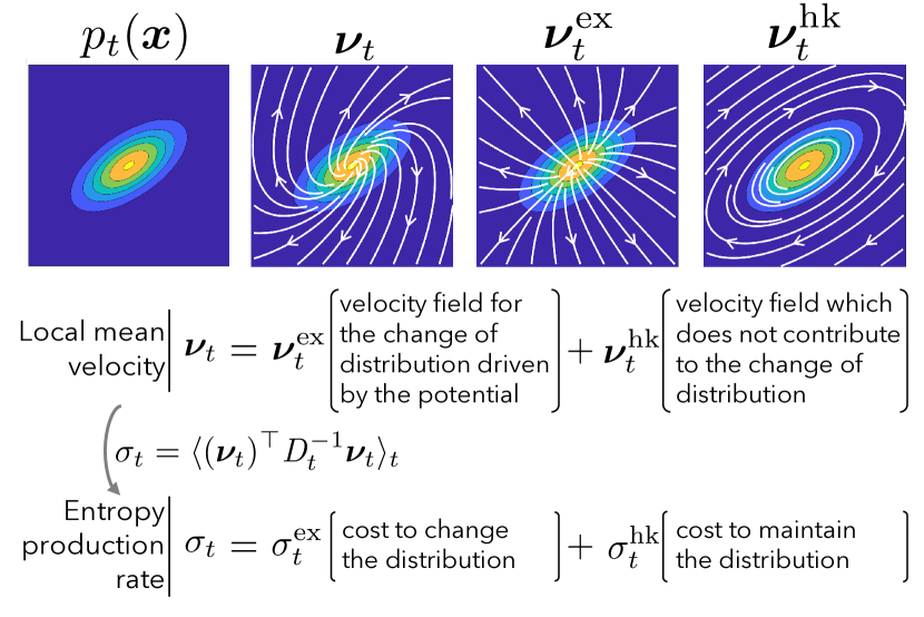
Figure 1: Schematic illustration of the geometric decomposition of the entropy production rate [41, 26]. Top: Illustration of the probability distribution $p_{t}(\bm{x})$ and the decomposition of the local mean velocity $\bm{\nu}_{t}$ in two-dimensional system. We can observe that the excess part of the local mean velocity $\bm{\nu}_{t}^{\mathrm{ex}}$ changes the probability distribution $p_{t}(\bm{x})$, while the housekeeping part of the local mean velocity $\bm{\nu}_{t}^{\mathrm{hk}}$ does not change the distribution. Bottom: The local mean velocity $\bm{\nu}_{t}$ can be decomposed into the excess part $\bm{\nu}_{t}^{\mathrm{ex}}$ and the housekeeping part $\bm{\nu}_{t}^{\mathrm{hk}}$ [Eq. (10)]. The entropy production rates corresponding to each local mean velocity are the expected values of the $L^{2}$-norm of them [Eqs. (4), (13) and (15)]. The orthogonality of the excess and housekeeping parts of the local mean velocity with respect to the expected value [Eq. (18)] gives a geometric decomposition of the entropy production rate into the excess and housekeeping parts [Eq. (9)].

The geometric decomposition is based on a decomposition of the local mean velocity $\bm{\nu}_{t}(\bm{x})$ into excess and housekeeping parts (Fig. 1):

$$\bm{\nu}_{t}(\bm{x})=\bm{\nu}_{t}^{\mathrm{ex}}(\bm{x})+\bm{\nu}_{t}^{\mathrm{hk}}(\bm{x})$$ (10)

Below, we explain the definitions of each term.

The excess entropy production rate $\sigma^{\mathrm{ex}}_{t}$ is defined using a local mean velocity $\bm{\nu}_{t}^{\mathrm{ex}}(\bm{x})$, which can be expressed as the gradient of some potential function $\phi_{t}(\bm{x})$,

$$\bm{\nu}_{t}^{\mathrm{ex}}(\bm{x}) =\mathit{D}_{t}\nabla\phi_{t}(\bm{x}),$$ (11)

and realizes the same time variation of the probability distribution $p_{t}(\bm{x})$ (Eq. 2) as the original local mean velocity $\bm{\nu}_{t}(\bm{x})$ (Eq. 3):

$$\partialderivative{p_{t}(\bm{x})}{t} =-\nabla\cdot\quantity[\bm{\nu}_{t}(\bm{x})p_{t}(\bm{x})]$$

$$=-\nabla\cdot\quantity[\bm{\nu}_{t}^{\mathrm{ex}}(\bm{x})p_{t}(\bm{x})].$$ (12)

In optimal transport theory, it is known that the velocity field $\bm{\nu}_{t}^{\mathrm{ex}}(\bm{x})$ which satisfies this condition, is uniquely introduced. The excess entropy production rate $\sigma^{\mathrm{ex}}_{t}(\bm{x})$ is defined using this local mean velocity $\bm{\nu}_{t}^{\mathrm{ex}}(\bm{x})$ as follows:

$$\sigma^{\mathrm{ex}}_{t}=\langle\quantity(\bm{\nu}_{t}^{\mathrm{ex}})^{\top}\mathit{D}_{t}^{-1}\bm{\nu}_{t}^{\mathrm{ex}}\rangle_{t}.$$ (13)

The housekeeping entropy production rate $\sigma^{\mathrm{hk}}_{t}$ is defined using the remaining local mean velocity

$$\bm{\nu}_{t}^{\mathrm{hk}}(\bm{x})=\bm{\nu}_{t}(\bm{x})-\bm{\nu}_{t}^{\mathrm{ex}}(\bm{x})$$ (14)

as

$$\sigma^{\mathrm{hk}}_{t}=\langle\quantity(\bm{\nu}_{t}^{\mathrm{hk}})^{\top}\mathit{D}_{t}^{-1}\bm{\nu}_{t}^{\mathrm{hk}}\rangle_{t}.$$ (15)

From Eq. (12), we can see that the housekeeping part of the local mean velocity does not change the probability distribution $p_{t}(\bm{x})$

$$0=-\nabla\cdot\quantity[\bm{\nu}_{t}^{\mathrm{hk}}(\bm{x})p_{t}(\bm{x})].$$ (16)

Hence, the housekeeping entropy production rate $\sigma^{\mathrm{hk}}_{t}$ is a thermodynamic cost which does not contribute to the time variation of the probability distribution $p_{t}(\bm{x})$. We remark that thermodynamic uncertainty relations [27], which provide a fundamental thermodynamic limit of accuracy, have been discussed for this housekeeping entropy production rate and the excess entropy production rate [47].

The sum of the excess entropy production rate $\sigma^{\mathrm{ex}}_{t}$ and the housekeeping entropy production rate $\sigma^{\mathrm{hk}}_{t}$ equals the total entropy production rate $\sigma_{t}$ [Eq. (9)]. This is because

$$\sigma_{t} =\langle\quantity(\bm{\nu}_{t}^{\mathrm{ex}}+\bm{\nu}_{t}^{\mathrm{hk}})^{\top}\mathit{D}_{t}^{-1}\quantity(\bm{\nu}_{t}^{\mathrm{ex}}+\bm{\nu}_{t}^{\mathrm{hk}})\rangle_{t}$$

$$=\sigma^{\mathrm{ex}}_{t}+\sigma^{\mathrm{hk}}_{t}+2\langle\quantity(\bm{\nu}_{t}^{\mathrm{ex}})^{\top}\mathit{D}_{t}^{-1}\bm{\nu}_{t}^{\mathrm{hk}}\rangle_{t}$$ (17)

and we find that

$$\langle\quantity(\bm{\nu}_{t}^{\mathrm{ex}})^{\top}\mathit{D}_{t}^{-1}\bm{\nu}_{t}^{\mathrm{hk}}\rangle_{t}= \int\quantity[(\nabla\phi_{t}(\bm{x}_{t}))^{\top}\bm{\nu}_{t}^{\mathrm{hk}}(\bm{x}_{t})p(\bm{x}_{t})]d\bm{x}_{t}$$

$$= -\int\phi_{t}(\bm{x}_{t})\nabla\cdot\quantity[\bm{\nu}_{t}^{\mathrm{hk}}(\bm{x}_{t})p(\bm{x}_{t})]d\bm{x}_{t}$$

$$= 0,$$ (18)

by using partial integration and Eq. (16), where we assumed $p_{t}(\bm{x})\to 0$ when $\|\bm{x}\|\to\infty$.

By definitions [Eqs. (13) and (15)], the excess and housekeeping entropy production rates are non-negative, $\sigma^{\rm ex}_{t}\geq 0$ and $\sigma^{\rm hk}_{t}\geq 0$. From the decomposition [Eq. (9)], we obtain that $\sigma_{t}\geq\sigma^{\rm ex}_{t}$ and $\sigma_{t}\geq\sigma^{\rm hk}_{t}$. Because the housekeeping entropy production rate $\sigma^{\mathrm{hk}}_{t}$ is a thermodynamic cost which does not contribute to $\partial p_{t}(\bm{x})/\partial t$, the inequality $\sigma_{t}\geq\sigma^{\rm ex}_{t}$ means that the excess entropy production rate $\sigma^{\mathrm{ex}}_{t}$ is the minimum entropy production rate for the fixed $\partial p_{t}(\bm{x})/\partial t$. Especially, when the noise covariance $\mathit{D}_{t}$ is a scalar matrix and written as $\mathit{D}_{t}=TI$ using the identity matrix $I$, the excess entropy production rate $\sigma^{\mathrm{ex}}_{t}$ can be written using the $L^{2}$-Wasserstein distance $\mathcal{W}_{2}$ [49] in the optimal transport theory [41, 21]:

$$\sigma^{\mathrm{ex}}_{t} =\min_{\bm{\nu}_{t}|\partial{p}_{t}/\partial t=-\nabla\cdot[\bm{\nu}_{t}p_{t}]}\frac{1}{T}\langle\|\bm{\nu}_{t}\|^{2}\rangle_{t}$$

$$=\frac{1}{T}\langle\|\nabla\phi_{t}\|^{2}\rangle_{t}$$

$$=\frac{1}{T}\lim_{\Delta t\to 0}\frac{\mathcal{W}_{2}\quantity(p_{t},p_{t+\Delta t})^{2}}{(\Delta t)^{2}}.$$ (19)

This expression is a consequence of the Benamou-Brenier formula [50] for an infinitesimal time interval in optimal transport theory [25, 41, 21]. This geometric interpretation of the excess entropy production rate leads to the thermodynamic speed limit, which is a fundamental thermodynamic limit on the speed [22, 25, 21].

We compare the geometric decomposition with the different decomposition introduced by Hatano and Sasa [48]. The decomposition introduced by Hatano and Sasa uses the steady state velocity field $\bm{\nu}_{t}^{\rm st}$ which satisfies $0=-\nabla\cdot\quantity[\bm{\nu}_{t}^{\mathrm{st}}(\bm{x})p^{\rm st}_{t}(\bm{x})]$ with the steady state distribution $p^{\rm st}_{t}(\bm{x})$. The housekeeping entropy production rate introduced by Hatano and Sasa is defined as $\sigma^{\rm hk;HS}_{t}=\langle(\bm{\nu}_{t}^{\mathrm{st}})^{\top}D_{t}^{-1}\bm{\nu}_{t}^{\mathrm{st}}\rangle_{t}$. Whereas $\sigma^{\rm hk;HS}_{t}$ depends on the steady-state distribution $p^{\rm st}_{t}(\bm{x})$, the housekeeping entropy production rate in a geometric decomposition $\sigma^{\rm hk}_{t}$ only depends on the current distribution $p_{t}(\bm{x})$. In general, $\sigma^{\rm hk;HS}_{t}$ is not equivalent to $\sigma^{\rm hk}_{t}$, and the inequality $\sigma^{\rm hk;HS}_{t}\geq\sigma^{\rm hk}_{t}$ holds [47]. In the steady state, the excess entropy production rate vanishes and the two housekeeping entropy production rates are equivalent to the entropy production rate $\sigma_{t}=\sigma^{\rm hk;HS}_{t}=\sigma^{\rm hk}_{t}$.

III Housekeeping and excess entropy production rates in Gaussian processes

III.1 Time-variation of probability distribution in Gaussian process

Here, we discuss a geometric decomposition for Gaussian processes. We prepare equations that capture the time variation of the probability distribution $p_{t}(\bm{x})$ under the assumption of Gaussian processes. We assume the following linear Langevin equation:

$$d\bm{x}_{t}=\mathit{D}_{t}[\mathit{A}_{t}\bm{x}_{t}+\bm{b}_{t}]dt+\sqrt{2}\mathit{G}_{t}d\bm{B}_{t}$$ (20)

where we set $\bm{f}_{t}(\bm{x}_{t})=\mathit{A}_{t}\bm{x}_{t}+\bm{b}_{t}$ with $d\times d$ matrix $\mathit{A}_{t}$ and $d$-dimensional vector $\bm{b}_{t}$ in Eq. (1). The corresponding Fokker-Planck equation is given by

$$\frac{\partial}{\partial t}p_{t}(\bm{x}) =-\nabla\cdot(\bm{\nu}_{t}(\bm{x})p_{t}(\bm{x})),$$

$$\bm{\nu}_{t}(\bm{x}) =D_{t}(\mathit{A}_{t}\bm{x}+\bm{b}_{t}-\nabla\ln p_{t}(\bm{x})).$$ (21)

We also assume that the initial probability distribution $p_{t}(\bm{x})$ is Gaussian. In the linear Langevin equations [Eq. (20)], if the initial probability distribution $p_{t}(\bm{x})$ is a Gaussian distribution and the noise term $d\bm{B}_{t}$ obeys the Gaussian distribution, then the future probability distribution $p_{t+\Delta t}(\bm{x})$ with $\Delta t>0$ keeps a Gaussian distribution. So, it is enough to follow the time variation of the mean $\bm{\mu}_{t}$ and the covariance matrix $\mathit{\Sigma}_{t}$ of the Gaussian distribution

$$p_{t}(\bm{x})=\frac{\exp\left[-\frac{1}{2}(\bm{x}-\bm{\mu}_{t})^{\top}\mathit{\Sigma}_{t}^{-1}(\bm{x}-\bm{\mu}_{t})\right]}{(2\pi)^{-\frac{d}{2}}\sqrt{\det\mathit{\Sigma}_{t}}}.$$ (22)

The time variation of the mean $\bm{\mu}_{t}$ and the covariance matrix $\mathit{\Sigma}_{t}$ in the Langevin equation [Eq. (20)] are given by

$$\dot{\bm{\mu}}_{t}= \frac{1}{dt}\mathbb{E}[d\bm{x}_{t}]$$

$$= \mathit{D}_{t}\mathit{A}_{t}\bm{\mu}_{t}+\mathit{D}_{t}\bm{b}_{t},$$ (23)

$$\dot{\mathit{\Sigma}}_{t}= \frac{1}{dt}\left(\mathbb{E}[(\bm{x}_{t+dt}-\bm{\mu}_{t+dt})(\bm{x}_{t+dt}-\bm{\mu}_{t+dt})^{\top}]\right.$$

$$-\left.\mathbb{E}[(\bm{x}_{t}-\bm{\mu}_{t})(\bm{x}_{t}-\bm{\mu}_{t})^{\top}]\right)$$

$$= \mathit{D}_{t}\mathit{A}_{t}\mathit{\Sigma}_{t}+\mathit{\Sigma}_{t}(\mathit{D}_{t}\mathit{A}_{t})^{\top}+2\mathit{D}_{t},$$ (24)

where we used $\mathbb{E}[\bm{x}_{t}]=\bm{\mu}_{t}$, $\mathbb{E}[(\bm{x}_{t}-\bm{\mu}_{t})(\bm{x}_{t}-\bm{\mu}_{t})^{\top}]=\mathit{\Sigma}_{t}$, $\mathbb{E}[d\bm{B}_{t}]=\bm{0}$ and $\mathbb{E}[d\bm{B}_{t}d\bm{B}_{s}^{\top}]=\delta(t-s)Idt$ and neglected the term $O(dt)$. Under the assumption of a Gaussian distribution, the time variation of the probability distribution $p_{t}(\bm{x})$ is equivalent to the following time variations of the mean $\bm{\mu}_{t}$ and the covariance matrix $\mathit{\Sigma}_{t}$. Thus, the condition of the steady state, which implies that the probability distribution does not change over time, can be rephrased as $\dot{\bm{\mu}}_{t}=0$ and $\dot{\mathit{\Sigma}}_{t}=0$. In the steady state, the equation for the covariance matrix [Eq. (24)] with $\dot{\mathit{\Sigma}}_{t}=0$ is called the Lyapunov equation.

III.2 Geometric decomposition of entropy production rate in Gaussian process

We discuss a geometric decomposition for Eq. (21) under the assumption of the Gaussian process. Under the assumption of the Gaussian process, the time variation by the excess part of the local mean velocity $\bm{\nu}_{t}^{\mathrm{ex}}(\bm{x})$ must provide the same time variation by $\bm{\nu}_{t}(\bm{x})$. Thus, $\bm{\nu}_{t}^{\mathrm{ex}}(\bm{x})$ must be a linear function of $\bm{x}$ because the process is Gaussian. Because $\nabla\ln p_{t}(\bm{x})=-\mathit{\Sigma}^{-1}_{t}(\bm{x}-\bm{\mu}_{t})$ is a linear function of $\bm{x}$, $\bm{\nu}_{t}^{\mathrm{ex}}(\bm{x})$ can be written as

$$\bm{\nu}_{t}^{\mathrm{ex}}(\bm{x}) =D_{t}\nabla\phi_{t}(\bm{x})$$

$$=\mathit{D}_{t}\mathit{A}_{t}^{\mathrm{ex}}\bm{x}+\mathit{D}_{t}\bm{b}_{t}^{\mathrm{ex}}-\mathit{D}_{t}\nabla\ln p_{t}(\bm{x}).$$ (25)

with some matrix $\mathit{A}_{t}^{\mathrm{ex}}$ and vector $\bm{b}_{t}^{\mathrm{ex}}$. We remark that $\bm{\nu}_{t}^{\mathrm{ex}}(\bm{x})$ cannot be generally written as Eq. (25) if $p_{t}(\bm{x})$ is not Gaussian.

Furthermore, $A^{\mathrm{ex}}_{t}$ is a symmetric matrix. This is because the excess part of the local mean velocity $\bm{\nu}_{t}^{\mathrm{ex}}(\bm{x})$ can be expressed using the gradient of some potential function $\phi_{t}(\bm{x})$. From the definition of $\bm{\nu}_{t}^{\mathrm{ex}}(\bm{x})$ [Eqs. (11) and (25)], we obtain

$$\nabla\phi_{t}(\bm{x})=\mathit{A}_{t}^{\mathrm{ex}}\bm{x}+\bm{b}_{t}^{\mathrm{ex}}-\nabla\ln p_{t}(\bm{x}).$$ (26)

The $i$-th component of this equation is:

$$\partialderivative{x_{i}}\phi_{t}(\bm{x})=\sum_{j}(\mathit{A}_{t}^{\mathrm{ex}})_{ij}x_{j}+b_{i}^{\mathrm{ex}}+\sum_{j}(\mathit{\Sigma_{t}}^{-1})_{ij}(x_{j}-(\mu_{t})_{j}).$$ (27)

Taking the derivative of this with respect to $x_{j}$ gives:

$$\partialderivative{x_{j}}\partialderivative{x_{i}}\phi_{t}(\bm{x})=(\mathit{A}_{t}^{\mathrm{ex}})_{ij}+(\mathit{\Sigma_{t}}^{-1})_{ij}.$$ (28)

Since $(\partial/\partial x_{j})(\partial/\partial x_{i})\phi_{t}(\bm{x})=(\partial/\partial x_{i})(\partial/\partial x_{j})\phi_{t}(\bm{x})$ and $\mathit{\Sigma}_{t}$ is symmetric matrix, we obtain $(A^{\rm ex}_{t})_{ij}=(A^{\rm ex}_{t})_{ji}$.

Because the excess part of the local mean velocity $\bm{\nu}_{t}^{\mathrm{ex}}(\bm{x})$ realizes the same time variation of the probability distribution as the original local mean velocity $\bm{\nu}_{t}(\bm{x})$, we obtain the time variation of the mean and the covariance matrix:

$$\dot{\bm{\mu}}_{t} =\mathit{D}_{t}\mathit{A}_{t}\bm{\mu}_{t}+\mathit{D}_{t}\bm{b}_{t}$$

$$=\mathit{D}_{t}\mathit{A}_{t}^{\mathrm{ex}}\bm{\mu}_{t}+\mathit{D}_{t}\bm{b}_{t}^{\mathrm{ex}},$$ (29)

$$\dot{\mathit{\Sigma}}_{t} =\mathit{D}_{t}\mathit{A}_{t}\mathit{\Sigma}_{t}+\mathit{\Sigma}_{t}(\mathit{D}_{t}\mathit{A}_{t})^{\top}+2\mathit{D}_{t}$$

$$=\mathit{D}_{t}\mathit{A}_{t}^{\mathrm{ex}}\mathit{\Sigma}_{t}+\mathit{\Sigma}_{t}(\mathit{D}_{t}\mathit{A}_{t}^{\mathrm{ex}})^{\top}+2\mathit{D}_{t}.$$ (30)

In the same way, we can rewrite the housekeeping part of the local mean velocity $\bm{\nu}_{t}^{\mathrm{hk}}(\bm{x})$ in Gaussian processes:

$$\bm{\nu}_{t}^{\mathrm{hk}}(\bm{x})=\mathit{D}_{t}\mathit{A}_{t}^{\mathrm{hk}}\bm{x}+\mathit{D}_{t}\bm{b}_{t}^{\mathrm{hk}},$$ (31)

where

$$\mathit{A}_{t}^{\mathrm{hk}} =\mathit{A}_{t}-\mathit{A}_{t}^{\mathrm{ex}},$$ (32)

$$\bm{b}_{t}^{\mathrm{hk}} =\bm{b}_{t}-\bm{b}_{t}^{\mathrm{ex}}.$$ (33)

From the equations for the time variation of the mean $\bm{\mu}_{t}$ [Eq. (29)] and the covariance matrix $\mathit{\Sigma}_{t}$ [Eq. (30)], we obtain

$$\bm{0} =\mathit{D}_{t}\mathit{A}_{t}^{\mathrm{hk}}\bm{\mu}_{t}+\mathit{D}_{t}\bm{b}_{t}^{\mathrm{hk}},$$ (34)

$$O =\mathit{D}_{t}\mathit{A}_{t}^{\mathrm{hk}}\mathit{\Sigma}_{t}+\mathit{\Sigma}_{t}(\mathit{D}_{t}\mathit{A}_{t}^{\mathrm{hk}})^{\top},$$ (35)

where $\bm{0}$ and $O$ are the zero vector and the zero matrix, respectively.

From these expressions of $\bm{\nu}_{t}(\bm{x})$, $\bm{\nu}^{\rm ex}_{t}(\bm{x})$ and $\bm{\nu}^{\rm hk}_{t}(\bm{x})$, we obtain analytical expressions of the entropy production rates for Gaussian processes,

$$\sigma_{t}= (\mathit{A}_{t}\bm{\mu}_{t}+\bm{b}_{t})^{\top}\mathit{D}_{t}(\mathit{A}_{t}\bm{\mu}_{t}+\bm{b}_{t})$$

$$+\tr\quantity[(\mathit{A}_{t}+\mathit{\Sigma}_{t}^{-1})^{\top}\mathit{D}_{t}(\mathit{A}_{t}+\mathit{\Sigma}_{t}^{-1})\mathit{\Sigma}_{t}],$$ (36)

$$\sigma_{t}^{\rm ex}= (\mathit{A}^{\rm ex}_{t}\bm{\mu}_{t}+\bm{b}^{\rm ex}_{t})^{\top}\mathit{D}_{t}(\mathit{A}^{\rm ex}_{t}\bm{\mu}_{t}+\bm{b}^{\rm ex}_{t})$$

$$+\tr\quantity[(\mathit{A}^{\rm ex}_{t}+\mathit{\Sigma}_{t}^{-1})^{\top}\mathit{D}_{t}(\mathit{A}^{\rm ex}_{t}+\mathit{\Sigma}_{t}^{-1})\mathit{\Sigma}_{t}],$$ (37)

$$\sigma^{\mathrm{hk}}_{t}= \tr\quantity[(\mathit{A}^{\rm hk}_{t})^{\top}\mathit{D}_{t}\mathit{A}^{\rm hk}_{t}\mathit{\Sigma}_{t}].$$ (38)

III.3 Geometric interpretations of entropy production rates

To understand the analytical expressions of the entropy production rates [Eqs. (36), (37) and (38)] from the viewpoint of geometry, we can introduce the Hilbert-Schmidt inner product. For any real-valued matrices $\mathit{Y}$ and $\mathit{Z}$, the Hilbert-Schmidt inner product is defined as $\langle\mathit{Y},\mathit{Z}\rangle_{\rm HS}=\tr[\mathit{Y}^{\top}\mathit{Z}]=\tr[\mathit{Z}^{\top}\mathit{Y}]$. For any vectors $\bm{y}$ and $\bm{z}$, the Hilbert-Schmidt inner product is regarded as the conventional inner product $\langle\bm{y},\bm{z}\rangle_{\rm HS}=\bm{y}^{\top}\bm{z}=\bm{z}^{\top}\bm{y}$. The Hilbert-Schmidt norm is introduced as $\|\mathit{Y}\|_{\rm HS}=\sqrt{\langle\mathit{Y},\mathit{Y}\rangle_{\rm HS}}$ and $L^{2}$-norm is introduced as $\|\bm{y}\|=\sqrt{\langle\bm{y},\bm{y}\rangle_{\rm HS}}$. Using the Hilbert-Schmidt norm and the $L^{2}$-norm, the entropy production rates are rewritten as

$$\sigma_{t}= \|\mathit{G}_{t}^{\top}(\mathit{A}_{t}\bm{\mu}_{t}+\bm{b}_{t})\|^{2}+\|\mathit{G}_{t}^{\top}(\mathit{A}_{t}+\mathit{\Sigma}_{t}^{-1})\sqrt{\mathit{\Sigma}_{t}}\|^{2}_{\rm HS},$$ (39)

$$\sigma_{t}^{\rm ex}= \|\mathit{G}_{t}^{\top}(\mathit{A}^{\rm ex}_{t}\bm{\mu}_{t}+\bm{b}^{\rm ex}_{t})\|^{2}+\|\mathit{G}_{t}^{\top}(\mathit{A}^{\rm ex}_{t}+\mathit{\Sigma}_{t}^{-1})\sqrt{\mathit{\Sigma}_{t}}\|^{2}_{\rm HS},$$ (40)

$$\sigma^{\mathrm{hk}}_{t}= \|\mathit{G}_{t}^{\top}\mathit{A}^{\rm hk}_{t}\sqrt{\mathit{\Sigma}_{t}}]\|^{2}_{\rm HS}.$$ (41)

These geometric interpretations as the Hilbert-Schmidt norm and the $L^{2}$-norm provide the non-negativity of the entropy production rates, $\sigma_{t}\geq 0$, $\sigma_{t}^{\rm ex}\geq 0$ and $\sigma_{t}^{\rm hk}\geq 0$.

Based on the geometric interpretations, we can check the validity of the geometric decomposition $\sigma_{t}=\sigma^{\rm ex}_{t}+\sigma_{t}^{\rm hk}$ as follows. From Eq. (34), we obtain an equivalence of the two $L^{2}$-norms,

$$\|\mathit{G}_{t}^{\top}(\mathit{A}_{t}\bm{\mu}_{t}+\bm{b}_{t})\|^{2}= \|\mathit{G}_{t}^{\top}(\mathit{A}^{\rm ex}_{t}\bm{\mu}_{t}+\bm{b}^{\rm ex}_{t})\|^{2}.$$ (42)

We can also obtain the orthogonality

$$\langle\mathit{G}_{t}^{\top}(\mathit{A}^{\rm ex}_{t}+\mathit{\Sigma}_{t}^{-1})\sqrt{\mathit{\Sigma}_{t}},\mathit{G}_{t}^{\top}\mathit{A}^{\rm hk}_{t}\sqrt{\mathit{\Sigma}_{t}}\rangle_{\rm HS}=0,$$ (43)

because we can calculate this Hilbert-Schmidt inner product as

$$\langle\mathit{G}_{t}^{\top}(\mathit{A}^{\rm ex}_{t}+\mathit{\Sigma}_{t}^{-1})\sqrt{\mathit{\Sigma}_{t}},\mathit{G}_{t}^{\top}\mathit{A}^{\rm hk}_{t}\sqrt{\mathit{\Sigma}_{t}}\rangle_{\rm HS}$$

$$=\tr[(\mathit{A}^{\rm ex}_{t}+\mathit{\Sigma}_{t}^{-1})^{\top}\mathit{D}_{t}\mathit{A}^{\rm hk}_{t}\mathit{\Sigma}_{t}]$$

$$=-\tr[\mathit{\Sigma}_{t}(\mathit{A}^{\rm hk}_{t})^{\top}\mathit{D}_{t}(\mathit{A}^{\rm ex}_{t}+\mathit{\Sigma}_{t}^{-1})]$$

$$=-\langle\mathit{G}_{t}^{\top}\mathit{A}^{\rm hk}_{t}\sqrt{\mathit{\Sigma}_{t}},\mathit{G}_{t}^{\top}(\mathit{A}^{\rm ex}_{t}+\mathit{\Sigma}_{t}^{-1})\sqrt{\mathit{\Sigma}_{t}}\rangle_{\rm HS}$$

$$=-\langle\mathit{G}_{t}^{\top}(\mathit{A}^{\rm ex}_{t}+\mathit{\Sigma}_{t}^{-1})\sqrt{\mathit{\Sigma}_{t}},\mathit{G}_{t}^{\top}\mathit{A}^{\rm hk}_{t}\sqrt{\mathit{\Sigma}_{t}}\rangle_{\rm HS},$$ (44)

where we used Eq. (35), $(\mathit{A}^{\rm ex}_{t})^{\top}=\mathit{A}^{\rm ex}_{t}$, $\mathit{D}_{t}=\mathit{G}_{t}\mathit{G}_{t}^{\top}$, $(\mathit{\Sigma}_{t}^{-1})^{\top}=\mathit{\Sigma}_{t}^{-1}$, $\mathit{D}_{t}^{\top}=\mathit{D}_{t}$ and the cyclic property of the trace. This orthogonality [Eq. (43)] provides a decomposition

$$\|\mathit{G}_{t}^{\top}(\mathit{A}_{t}+\mathit{\Sigma}_{t}^{-1})\sqrt{\mathit{\Sigma}_{t}}\|^{2}_{\rm HS}$$

$$=\|\mathit{G}_{t}^{\top}(\mathit{A}^{\rm ex}_{t}+\mathit{\Sigma}_{t}^{-1})\sqrt{\mathit{\Sigma}_{t}}\|^{2}_{\rm HS}+\|\mathit{G}_{t}^{\top}\mathit{A}^{\rm hk}_{t}\sqrt{\mathit{\Sigma}_{t}}]\|^{2}_{\rm HS},$$ (45)

where we used the Pythagorean theorem $\langle Y+Z,Y+Z\rangle_{\rm HS}=\langle Y,Y\rangle_{\rm HS}+\langle Z,Z\rangle_{\rm HS}$ with $\langle Y,Z\rangle_{\rm HS}=0$ by adopting $Y=\mathit{G}_{t}^{\top}(\mathit{A}^{\rm ex}_{t}+\mathit{\Sigma}_{t}^{-1})\sqrt{\mathit{\Sigma}_{t}}$ and $Z=\mathit{G}_{t}^{\top}\mathit{A}^{\rm hk}_{t}\sqrt{\mathit{\Sigma}_{t}}$. By combining two geometric relations (42) and (45), we obtain the geometric decomposition $\sigma_{t}=\sigma^{\rm ex}_{t}+\sigma_{t}^{\rm hk}$.

IV Oscillatory mode decomposition of virtual dynamics given by $\bm{\nu}_{t}^{\mathrm{hk}}$

In preparation for the derivation of the main results in the next section, we show that the housekeeping part of the local mean velocity $\bm{\nu}_{t}^{\mathrm{hk}}(\bm{x})$ in Eq. (31) reflects oscillatory dynamics. To observe this, we consider the following virtual deterministic process:

$$d\bm{x}_{s}=\quantity[\mathit{D}_{t}\mathit{A}_{t}^{\mathrm{hk}}\bm{x}_{s}+\mathit{D}_{t}\bm{b}_{t}^{\mathrm{hk}}]ds=\bm{\nu}_{t}^{\mathrm{hk}}(\bm{x}_{s})ds.$$ (46)

where the housekeeping part of the local mean velocity $\bm{\nu}_{t}^{\mathrm{hk}}(\bm{x})$ is introduced by the original process [Eq. (20)]. Here, $s$ stands for the time of the virtual dynamics, whereas $t$ stands for the time of the original Langevin dynamics [Eq. (20)]. During the virtual deterministic processes, the function $\bm{\nu}_{t}^{\mathrm{hk}}(\bm{x})$ is fixed with respect to changes in $s$. We here consider the continuity equation $\partial q_{s}(\bm{x})/\partial s=-\nabla\cdot(\bm{\nu}_{t}^{\mathrm{hk}}(\bm{x})q_{s}(\bm{x}))$ for the time variation of the probability distribution $q_{s}(\bm{x})$ for this deterministic virtual process. If $q_{s}(\bm{x})$ is given by the same distribution in the original dynamics $p_{t}(\bm{x})$, $\left.\partial q_{s}(\bm{x})/\partial s\right|_{q_{s}(\bm{x})=p_{t}(\bm{x})}=-\nabla\cdot(\bm{\nu}_{t}^{\mathrm{hk}}(\bm{x})p_{t}(\bm{x}))=0$. This fact implies that $p_{t}(\bm{x})$ is the invariant measure of this virtual deterministic process [Eq. (46)].

We discuss the analytical solution for the future state $\bm{x}_{t+\Delta s}$ with $\Delta t>0$ in the virtual deterministic process [Eq. (46)]. From Eq. (34) and $d\bm{\mu}_{t}/ds=\bm{0}$, we obtain $d[\bm{x}_{s}-\bm{\mu}_{t}]/ds=\mathit{D}_{t}\mathit{A}_{t}^{\mathrm{hk}}\quantity[\bm{x}_{s}-\bm{\mu}_{t}]$, and thus

$$\bm{x}_{s+\Delta t} =\bm{\mu}_{t}+e^{\mathit{D}_{t}A_{t}^{\mathrm{hk}}\Delta t}\quantity(\bm{x}_{s}-\bm{\mu}_{t})$$

$$=\bm{\mu}_{t}+\sum_{k}e^{\lambda_{k}\Delta t}\mathsf{F}_{k}\quantity(\bm{x}_{s}-\bm{\mu}_{t})$$

$$=\bm{\mu}_{t}+\sum_{k}e^{2\pi\chi_{k}\mathrm{i}\Delta t}\mathsf{F}_{k}\quantity(\bm{x}_{s}-\bm{\mu}_{t}).$$ (47)

Here, $\lambda_{k}$ is the $k$-th eigenvalue of $\mathit{D}_{t}A_{t}^{\mathrm{hk}}$ and $\chi_{k}$ is defined as

$$\chi_{k}=\lambda_{k}/(2\pi\mathrm{i}),$$ (48)

where $\mathrm{i}$ stands for the imaginary unit. As proven later, $\lambda_{k}$ is purely imaginary, and hence, $\chi_{k}$ is a real number. $\mathsf{F}_{k}$ is the projection matrix that provides the spectral decomposition of $\mathit{D}_{t}A_{t}^{\mathrm{hk}}$,

$$\mathit{D}_{t}A_{t}^{\mathrm{hk}}=\sum_{k}\lambda_{k}\mathsf{F}_{k}.$$ (49)

This projection matrix $\mathsf{F}_{k}$ is introduced using the eigenvalue decomposition of $\mathit{D}_{t}A_{t}^{\mathrm{hk}}$ as $\mathit{D}_{t}A_{t}^{\mathrm{hk}}=\mathsf{P}\Lambda\mathsf{P}^{-1}$, where $\mathsf{P}$ is a matrix of eigenvectors, and $\Lambda$ is a diagonal matrix whose $k$-th element is the $k$-th eigenvalue $\lambda_{k}$. Let $\bm{e}_{k}$ be the $k$-th basic unit vector, whose $k$-th element is $1$ and all other elements are $0$. This projection matrix $\mathsf{F}_{k}$ is explicitly defined as

$$\mathsf{F}_{k}:=\mathsf{P}\bm{e}_{k}\bm{e}_{k}^{\top}\mathsf{P}^{-1},$$ (50)

and the eigenvalue decomposition was rewritten as Eq. (49).

The time evolution of the virtual dynamics [Eq. (47)] is rewritten as the time evolution of the modes. Since $\sum_{k}\bm{e}_{k}\bm{e}_{k}^{\top}=\mathit{I}$, the projection matrix satisfies $\sum_{k}\mathsf{F}_{k}=I$. Thus, $\bm{x}_{s}-\bm{\mu}_{t}$ can be decomposed as the sum of the modes $\mathsf{F}_{k}\quantity(\bm{x}_{s}-\bm{\mu}_{t})$,

$$\bm{x}_{s}-\bm{\mu}_{t}=\sum_{k}\mathsf{F}_{k}\quantity(\bm{x}_{s}-\bm{\mu}_{t}),$$ (51)

and thus Eq. (47) reads the time evolution of the modes

$$\sum_{k}\mathsf{F}_{k}(\bm{x}_{s+\Delta t}-\bm{\mu}_{t}) =\sum_{k}e^{2\pi\chi_{k}\mathrm{i}\Delta t}\mathsf{F}_{k}\quantity(\bm{x}_{s}-\bm{\mu}_{t}),$$ (52)

where we used $\sum_{k}\mathsf{F}_{k}(\bm{x}_{s+\Delta t}-\bm{\mu}_{t})=\bm{x}_{s+\Delta t}-\bm{\mu}_{t}$. We can also show that each mode evolves independently as follows,

$$\mathsf{F}_{k}\quantity(\bm{x}_{s+\Delta t}-\bm{\mu}_{t})=e^{2\pi\chi_{k}\mathrm{i}\Delta t}\mathsf{F}_{k}\quantity(\bm{x}_{s}-\bm{\mu}_{t}),$$ (53)

where we multiplied both sides of Eq. (52) by $\mathsf{F}_{k}$ from the left, and used a mathematical property of the projection matrix $\mathsf{F}_{k}\mathsf{F}_{j}=\delta_{kj}\mathsf{F}_{k}$.

Because the eigenvalues of $\mathit{D}_{t}\mathit{A}_{t}^{\mathrm{hk}}$ are $0$ or purely imaginary, the mode $\mathsf{F}_{k}\quantity(\bm{x}_{s}-\bm{\mu}_{t})$ can be regarded as the oscillation mode. To show this fact, we use Eq. (35), and $A_{t}^{\mathrm{hk}}$ can be written as

$$\mathit{D}_{t}\mathit{A}_{t}^{\mathrm{hk}}=\mathit{Q}\mathit{\Sigma}_{t}^{-1}$$ (54)

with an anti-symmetric matrix $\mathit{Q}=-\mathit{Q}^{\top}$. By denoting the eigenvalues of a matrix $X$ as $\mathrm{eig}(X)$, the eigenvalues $\mathit{D}_{t}\mathit{A}_{t}^{\mathrm{hk}}$ can be written as

$$\mathrm{eig}\quantity(\mathit{D}_{t}\mathit{A}_{t}^{\mathrm{hk}})=\mathrm{eig}\quantity(\mathit{Q}\mathit{\Sigma}_{t}^{-1})=\mathrm{eig}\quantity((\sqrt{\mathit{\Sigma}_{t}})^{-1}\mathit{Q}(\sqrt{\mathit{\Sigma}_{t}})^{-1}),$$ (55)

where we used the fact that $\mathrm{eig}(XY)=\mathrm{eig}(YX)$ for any pair of matrices $X$ and $Y$. Since $(\sqrt{\mathit{\Sigma}_{t}})^{-1}\mathit{Q}(\sqrt{\mathit{\Sigma}_{t}})^{-1}$ is an anti-symmetric matrix, and the eigenvalues of an anti-symmetric matrix are $0$ or purely imaginary, the eigenvalues of $\mathit{D}_{t}A_{t}^{\mathrm{hk}}$ are also $0$ or purely imaginary. This implies that $\chi_{k}=\lambda_{k}/(2\pi\mathrm{i})$ is a real number. Hence, Eq. (53) means that the $k$-th mode $\mathsf{F}_{k}\quantity(\bm{x}_{s}-\bm{\mu}_{t})$ oscillates with the frequency $\chi_{k}$, and Eq. (47) means that the time evolution of the virtual dynamics is given by the sum of the oscillation modes.

Further, we discuss the intensity of the oscillation mode in the original process [Eq. (20)]. By replacing $\bm{x}_{s}$ with $\bm{x}_{t}$ in $\mathsf{F}_{k}\quantity(\bm{x}_{s}-\bm{\mu}_{t})$, we introduce the $k$-th oscillation mode $\mathsf{F}_{k}\quantity(\bm{x}_{t}-\bm{\mu}_{t})$ in the original process. The intensity of the $k$-th mode is introduced as the expected value of the square of the Hilbert-Schmidt norm:

$$\langle\|\mathsf{F}_{k}(\bm{x}_{t}-\bm{\mu}_{t})\|^{2}_{\rm HS}\rangle_{t} =\tr[[\mathsf{F}_{k}(\bm{x}_{t}-\bm{\mu}_{t})]^{*}\mathsf{F}_{k}(\bm{x}_{t}-\bm{\mu}_{t})]$$

$$=\tr({\mathsf{F}_{k}\mathit{\Sigma}_{t}\mathsf{F}_{k}^{*}}),$$ (56)

where the symbol ^∗ stands for the conjugate transpose of the matrix and the Hilbert-Schmidt norm for the complex matrix $Y$ is defined as $\|Y\|_{\rm HS}=\sqrt{\tr(Y^{*}Y)}$. We remark that this value $\tr({\mathsf{F}_{k}\mathit{\Sigma}_{t}\mathsf{F}_{k}^{*}})$ is also regarded as the intensity of the oscillation mode in the virtual deterministic process,

$$\langle\|\mathsf{F}_{k}(\bm{x}_{s}-\bm{\mu}_{t})\|^{2}_{\rm HS}\rangle_{\rm inv} =\langle\|\mathsf{F}_{k}(\bm{x}_{t}-\bm{\mu}_{t})\|^{2}_{\rm HS}\rangle_{t}$$

$$=\tr({\mathsf{F}_{k}\mathit{\Sigma}_{t}\mathsf{F}_{k}^{*}}),$$ (57)

where $\langle\cdots\rangle_{\rm inv}$ is the expectation with respect to the invariant measure $p_{t}$ defined as $\langle\cdots\rangle_{\rm inv}=\int d\bm{x}_{s}p_{t}(\bm{x}_{s})\cdots$.

We also introduce the $i$-th intensity of the $k$-th oscillation mode by considering each diagonal element of the matrix $\mathsf{F}_{k}\mathit{\Sigma}_{t}\mathsf{F}_{k}^{*}$. The $i$-th intensity of the $k$-th oscillation mode is computed as the expected value of the square of the norm:

$$\langle\|(\mathsf{F}_{k}\quantity(\bm{x}_{t}-\bm{\mu}_{t}))_{i}\|^{2}\rangle_{t} =\langle\|(\mathsf{F}_{k}\quantity(\bm{x}_{s}-\bm{\mu}_{t}))_{i}\|^{2}\rangle_{\rm inv}$$

$$=(\mathsf{F}_{k}\mathit{\Sigma}_{t}\mathsf{F}_{k}^{*})_{ii}.$$ (58)

V Mode decomposition of the housekeeping entropy production rate via oscillation modes

V.1 Main result

As the main result of this paper, we derived a decomposition of the housekeeping entropy production rate into independent positive contributions for each oscillation mode:

$$\sigma^{\mathrm{hk}}_{t} =(2\pi)^{2}\sum_{k}\chi_{k}^{2}\tr(\mathit{G}_{t}^{-1}\mathsf{F}_{k}\mathit{\Sigma}_{t}\mathsf{F}_{k}^{*}(\mathit{G}_{t}^{-1})^{\top})$$

$$=(2\pi)^{2}\sum_{k}\chi_{k}^{2}\|\mathit{G}_{t}^{-1}\mathsf{F}_{k}\sqrt{\mathit{\Sigma}_{t}}\|^{2}_{\rm HS},$$ (59)

where we assume that the eigenvalues of $D_{t}\mathit{A}_{t}^{\mathrm{hk}}$ are not degenerate. Because the Hilbert-Schmidt norm $\|\mathit{G}_{t}^{-1}\mathsf{F}_{k}\sqrt{\mathit{\Sigma}_{t}}\|_{\rm HS}$ is non-negative, we can see that the housekeeping entropy production rate can be decomposed into independent positive contributions from each oscillation mode.

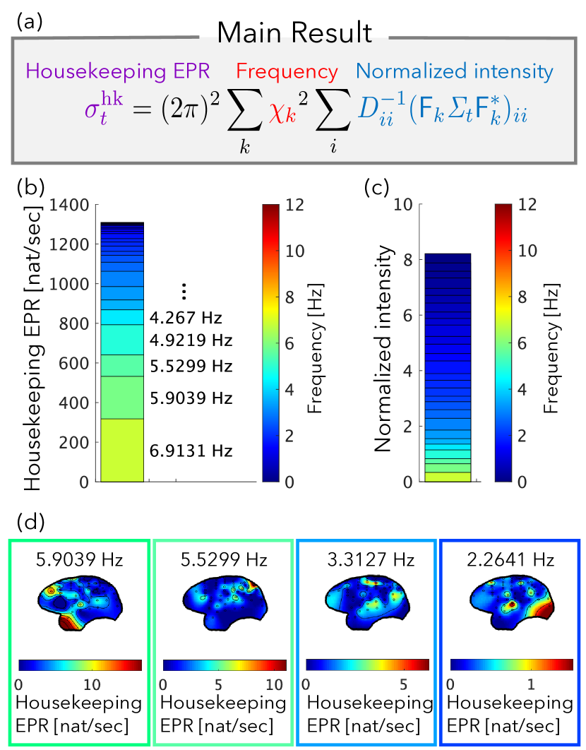
Figure 2: An application example of our decomposition [Eq. (68)] to ECoG data. (a) Our decomposition of the housekeeping entropy production rate (EPR) [Eq. (60)]. The housekeeping entropy production rate can be decomposed into the contributions of each oscillatory mode, which are the products of the squared frequency and the normalized intensity. (b) An example of our decomposition with respect to each oscillatory mode. The stacked bar graph shows the contributions of each oscillatory mode $\sigma_{t}^{\mathrm{hk}(k)}$ in Eq. (72). The colors represent the frequency $\chi_{k}$. The sum of these contributions represents the total housekeeping entropy production rate $\sigma_{t}^{\mathrm{hk}}$. (c) The normalized intensity $J_{k}$ [Eq. (73)] for comparison. (d) Spatial distribution of contributions to the housekeeping entropy production rate for each oscillation mode $\bm{\sigma}_{t}^{\mathrm{hk}(k)}$ [Eq. (71)]. Each element of $\bm{\sigma}_{t}^{\mathrm{hk}(k)}$ is represented by the color at the location of each electrode. Each plot shows the brain viewed from the lateral side.

When the noise coefficient $\mathit{G}_{t}$ is a diagonal matrix, the meaning of the mode decomposition is more evident (Fig. 2a):

$$\sigma^{\mathrm{hk}}_{t}=(2\pi)^{2}\sum_{k}\chi_{k}^{2}\sum_{i}D_{ii}^{-1}(\mathsf{F}_{k}\mathit{\Sigma}_{t}\mathsf{F}_{k}^{*})_{ii}.$$ (60)

Recall that the diagonal elements of $\mathsf{F}_{k}\Sigma\mathsf{F}_{k}^{*}$ correspond to the intensity of the $k$-th oscillation mode [(Eq. 58)].

$$D_{ii}^{-1}(\mathsf{F}_{k}\mathit{\Sigma}_{t}\mathsf{F}_{k}^{*})_{ii}$$ (61)

is the intensity normalized by the diffusion matrix $D$. As discussed, $\chi_{k}$ corresponds to the frequency of oscillation. Hence, we can see that the contributions of each oscillatory mode to the housekeeping entropy production rate can be written by contributions of the normalized intensity and the square of the frequency of the oscillation. In other words, oscillation modes with higher frequency and normalized intensity contribute more to the housekeeping entropy production rate. We also remark that the normalized intensity is attributed to $\mathit{\Sigma}_{t}$, which determines the spatial shape of the probability distribution $p_{t}(\bm{x})$.

Since the normalized intensity is attributed to each element of $\bm{x}_{t}$, we can also examine the spatial distribution of the source of the housekeeping entropy production rate.

V.2 Derivation of the main result

From the analytical expression of the housekeeping entropy production rate [Eq. (38)] and the eigenvalue decomposition of $\mathit{D}_{t}\mathit{A}_{t}^{\mathrm{hk}}$ [Eq. (49)], we obtain

$$\sigma^{\mathrm{hk}}_{t} =\tr\quantity((\mathit{A}_{t}^{\mathrm{hk}})^{\top}\mathit{D}_{t}\mathit{A}_{t}^{\mathrm{hk}}\mathit{\Sigma}_{t})$$

$$=\tr\quantity(\mathit{G}_{t}^{-1}\quantity(\mathit{D}_{t}\mathit{A}_{t}^{\mathrm{hk}})\mathit{\Sigma}_{t}\quantity(\mathit{D}_{t}\mathit{A}_{t}^{\mathrm{hk}})^{*}(\mathit{G}_{t}^{-1})^{\top})$$

$$=\sum_{kl}\lambda_{k}\overline{\lambda_{l}}\tr\quantity(\mathit{G}_{t}^{-1}\mathsf{F}_{k}\mathit{\Sigma}_{t}\mathsf{F}_{l}^{*}(\mathit{G}_{t}^{-1})^{\top}),$$ (62)

where $\overline{\lambda_{l}}$ stands for the complex conjugate of $\lambda_{l}$. From Eq. (35) and the eigenvalue decomposition of $\mathit{D}_{t}\mathit{A}_{t}^{\mathrm{hk}}$ [Eq. (49)], we obtain

$$0 =\sum_{m}\quantity[\lambda_{m}\mathsf{F}_{m}\mathit{\Sigma}_{t}+\overline{\lambda_{m}}\mathit{\Sigma}_{t}\mathsf{F}_{m}^{*}]$$

$$=\sum_{m}\lambda_{m}\quantity[\mathsf{F}_{m}\mathit{\Sigma}_{t}-\mathit{\Sigma}_{t}\mathsf{F}_{m}^{*}],$$ (63)

where we used the fact that the eigenvalue $\lambda_{m}$ is purely imaginary. By multiplying $\mathsf{F}_{k}$ from the left side and $\mathsf{F}_{l}^{*}$ from the right side and using the property of the projection matrix $\mathsf{F}_{k}\mathsf{F}_{j}=\delta_{kj}\mathsf{F}_{k}$, we obtain

$$0 =\lambda_{k}\mathsf{F}_{k}\mathit{\Sigma}_{t}\mathsf{F}_{l}^{*}-\lambda_{l}\mathsf{F}_{k}\mathit{\Sigma}_{t}\mathsf{F}_{l}^{*}$$

$$=(\lambda_{k}-\lambda_{l})\mathsf{F}_{k}\mathit{\Sigma}_{t}\mathsf{F}_{l}^{*}.$$ (64)

This equation means that $\mathsf{F}_{k}\Sigma\mathsf{F}_{l}^{*}=0$ when $\lambda_{k}\neq\lambda_{l}$. From the assumption that the eigenvalues of $\mathit{D}_{t}\mathit{A}_{t}^{\mathrm{hk}}$ are not degenerate, we obtain $\mathsf{F}_{k}\Sigma\mathsf{F}_{l}^{*}=\delta_{kl}\mathsf{F}_{k}\Sigma\mathsf{F}_{k}^{*}$ because $\lambda_{k}\neq\lambda_{l}$ when $k\neq l$. Thus, Eq. (62) can be rewritten as

$$\sigma^{\mathrm{hk}}_{t} =\sum_{k}|\lambda_{k}|^{2}\tr\quantity(\mathit{G}_{t}^{-1}\mathsf{F}_{k}\mathit{\Sigma}_{t}\mathsf{F}_{k}^{*}(\mathit{G}_{t}^{-1})^{\top})$$

$$=(2\pi)^{2}\sum_{k}\chi_{k}^{2}\tr\quantity(\mathit{G}_{t}^{-1}\mathsf{F}_{k}\mathit{\Sigma}_{t}\mathsf{F}_{k}^{*}(\mathit{G}_{t}^{-1})^{\top}),$$ (65)

which is our main result [Eq. (59)], where $|\cdot|$ stands for the absolute value.

We remark that our result can be generalized without the assumption of the non-degeneracy by using the fact that $\mathsf{F}_{k}\Sigma\mathsf{F}_{l}^{*}=0$ when $\lambda_{k}\neq\lambda_{l}$. If $\mathit{D}_{t}\mathit{A}_{t}^{\mathrm{hk}}$ are degenerate, the housekeeping entropy production rate [Eq. (62)] is calculated as

$$\sigma^{\mathrm{hk}}_{t}=\sum_{i\in\mathcal{M}_{\rm I}}\sum_{k\in\mathcal{D}(i)}\sum_{l\in\mathcal{D}(i)}|\lambda_{i}|^{2}\tr\quantity(\mathit{G}_{t}^{-1}\mathsf{F}_{k}\mathit{\Sigma}_{t}\mathsf{F}_{l}^{*}(\mathit{G}_{t}^{-1})^{\top}),$$ (66)

where $\mathcal{M}_{\rm I}$ is the set of the independent modes such that $\lambda_{i}\neq\lambda_{i^{\prime}}$ for any $i\in\mathcal{M}_{\rm I}$, $i^{\prime}\in\mathcal{M}_{\rm I}$, and $\mathcal{D}(i)$ is the set of the $i$-th degenerate modes such that $\lambda_{k}=\lambda_{k^{\prime}}$ for any $k\in\mathcal{D}(i)$, $k^{\prime}\in\mathcal{D}(i)$. Thus, we obtain a similar expression

$$\sigma^{\mathrm{hk}}_{t}=(2\pi)^{2}\sum_{i\in\mathcal{M}_{\rm I}}\chi_{i}^{2}\tr\quantity(\mathit{G}_{t}^{-1}\tilde{\mathsf{F}}_{i}\mathit{\Sigma}_{t}\tilde{\mathsf{F}}_{i}^{*}(\mathit{G}_{t}^{-1})^{\top}),$$ (67)

where $\tilde{\mathsf{F}}_{i}=\sum_{k\in\mathcal{D}(i)}\mathsf{F}_{k}$.

V.3 Interpretation and possible applications to data analysis

In this subsection, we provide an interpretation of our decomposition [Eq. (60)] and define several quantities in preparation for the data analysis in the next section.

To clarify that the proposed decomposition can be simultaneously decomposed in terms of both oscillatory mode and dimension, we introduce the following quantities:

$$\sigma_{t}^{\mathrm{hk}} =\sum_{i}\sum_{k}\sigma_{t}^{\mathrm{hk}(k,i)},$$ (68)

$$\sigma_{t}^{\mathrm{hk}(k,i)} =(2\pi\chi_{k})^{2}J_{k}^{(i)},$$ (69)

$$J_{k}^{(i)} =D_{ii}^{-1}(\mathit{F}_{k}\mathit{\Sigma}_{t}\mathit{F}_{k}^{*})_{ii}.$$ (70)

First, in Eq. (68), the housekeeping entropy production rate is decomposed into the sum of the contributions of the $i$-th dimension of the $k$-th oscillatory mode, $\sigma_{t}^{\mathrm{hk}(k,i)}$. Then, in Eq. (69), $\sigma_{t}^{{\mathrm{hk}},(k,i)}$ is expressed using the product of the square of the frequency of the $k$-th oscillatory mode, $\chi_{k}$, and the normalized intensity of the $i$-th dimension of the $k$-th oscillatory mode $J_{k}^{(i)}$. Finally, in Eq. (70), $J_{k}^{(i)}$ is the intensity of the $i$-th dimension of the $k$-th oscillatory mode $(\mathit{F}_{k}\mathit{\Sigma}_{t}\mathit{F}_{k}^{*})_{ii}$ divided by the $i$-th diagonal element of the diffusion matrix $D_{ii}$.

In applications to the neural data analysis in this study, the dimension $i$ corresponds to the electrodes of the ECoG recordings. Since the spatial positions of the electrodes are given, we can consider the decomposition [Eq. (68)] as the spatio-temporal decomposition. Then, $\sigma_{t}^{\mathrm{hk}(k,i)}$ is the contribution of the $i$-th electrode of the $k$-th oscillatory mode. As will be shown later in Fig. 2d, this enable us to plot the spatial distribution of contributions to the housekeeping entropy production rate. The spatial distribution of contributions from the $k$-th oscillatory mode is expressed as the vector

$$\bm{\sigma}_{t}^{\mathrm{hk}(k)}=(\sigma_{t}^{\mathrm{hk}(k,i=1)},\sigma_{t}^{\mathrm{hk}(k,i=2)},\cdots,\sigma_{t}^{\mathrm{hk}(k,i=d)}).$$ (71)

Additionally, we prepare some quantities for next section.

$$\sigma_{t}^{\mathrm{hk}(k)} =\sum_{i}\sigma_{t}^{\mathrm{hk}(k,i)}=(2\pi\chi_{k})^{2}J_{k},$$ (72)

$$J_{k} =\sum_{i}J_{k}^{(i)},$$ (73)

where $\sigma_{t}^{\mathrm{hk}(k)}$ is a contribution of the $k$-th oscillatory mode and defined as the sum of $\sigma_{t}^{\mathrm{hk}(k,i)}$ over dimension $i$ [Eq. (72)]. Note that the sum of $\sigma_{t}^{\mathrm{hk}(k)}$ over oscillatory modes $k$ recovers the total housekeeping entropy production rate: $\sigma_{t}^{\mathrm{hk}}=\sum_{k}\sigma_{t}^{\mathrm{hk}(k)}$ [Eq. (68)]. Here, $J_{k}$ is the sum of the normalized intensity $J_{k}^{(i)}$ over the dimension [Eq. (73)], and $\sigma_{t}^{\mathrm{hk}(k)}$ is written using a product of square of the frequency $\chi_{k}$ and $J_{k}$ [Eq. (72)].

VI Application to ECoG Data

VI.1 Examples of results from a single time window in one recording session of a monkey

To demonstrate the utility of our mode decomposition of the housekeeping entropy production rate, we applied it to neural data and compared the properties of the decomposition during awake and anesthetized conditions. We used a 128-channel ECoG open dataset recorded from monkey [42]. Details of the preprocessing and data analysis are explained in the Methods section. After the preprocessing, the number of channels becomes 64 since we applied bipolar rereference as a preprocessing to remove common artifacts across electrodes. The data were recorded during awake eyes opened, awake eyes closed, and ketamine-medetomidine-induced anesthetized conditions. It is well known that the Fourier power of the delta wave (0.5-4 Hz) increases during anesthetized condition [43]. We compared how contributions of each frequency band to the housekeeping entropy production rate vary depending on these conditions with different oscillatory properties. Note that we fit the multivariate time series of ECoG signals to the linear Langevin equation (20) with the noise coefficient matrix $D_{t}$ being a diagonal matrix. We used the linear autoregressive model as a reasonable model based on the previous finding that the linear autoregressive model outperforms other nonlinear models in terms of r-squared when fitting ECoG time series data [51].

We divided the data into 60-second time windows and calculated the housekeeping entropy production rate for each 60-second time window. We assume piecewise stationarity for each time window to calculate the housekeeping entropy production rate. This assumption means that the system is in a steady state only within each 60-second time window, but a steady state can vary across time windows. This assumption can be justified if the system quickly relaxes to a steady state in response to changes in the environment, and this steady state slowly changes due to changes in the environment. In our analysis, the housekeeping entropy production rate is equivalent to the entropy production rate because the system is assumed to be in a steady state within each time window.

We exemplify an application of our decomposition, using a certain 60-second time window of ECoG multivariate time series recorded in a monkey during awake eyes closed condition (Fig. 2). The result of the application of our decomposition is illustrated in Fig. 2b. There are 64 modes, including plus and minus frequencies, which is equal to the number of the channels. In Fig. 2b, the modes with the same absolute values of frequencies are combined and shown as a single mode. Hence, 32 modes are shown in the Fig. 2b. The exact number of modes is different among individual monkeys depending on the number of electrodes discarded in preprocessing. The stacked bar graph shows contributions from each oscillatory mode $\sigma_{t}^{\mathrm{hk}(k)}$. The sum of these contributions represents the total housekeeping entropy production rate $\sigma_{t}^{\mathrm{hk}}$. We observed the amounts of contributions to the housekeeping entropy production rate from 6.9131 Hz component, 5.9039 Hz component and so on.

Our decomposition is different from just plotting the normalized intensity of the oscillation $J_{k}$ in Eq. (73) (Fig. 2c). Compared to simply plotting the normalized intensity of the oscillation $J_{k}$ (Fig. 2c), $\sigma_{t}^{\mathrm{hk}(k)}$ of high frequency components are emphasized and $\sigma_{t}^{\mathrm{hk}(k)}$ of low frequency components are diminished (Fig. 2b) because the squares of the frequencies $\chi_{k}$ are multiplied in $\sigma_{t}^{\mathrm{hk}(k)}$ [Eq. (72)].

The decomposition in Eq. (68) also allows us to plot the spatial distribution of the contributions to the entropy production rate from each oscillatory mode $\bm{\sigma}_{t}^{\mathrm{hk}(k)}$ (Fig. 2d) [Eq. (71)]. This is because the decomposition is not only a decomposition into oscillatory elements but also a decomposition into the contributions from each dimension of the spatial oscillation mode [Eq. (68)]. In Fig. 2d, each element of $\bm{\sigma}_{t}^{\mathrm{hk}(k)}$ was represented by the color at the location of each electrode, and the values between electrode positions were interpolated using the ft_topoplotER function from FieldTrip [52].

VI.2 Temporal stability of the decomposition

Before investigating the difference across conditions, we first assessed how stable the decomposition of the housekeeping entropy production rate $\sigma_{t}^{\mathrm{hk}(k)}$ is over time (Fig. 3). We found that the proportion of contribution to the housekeeping entropy production rate from each frequency $\sigma_{t}^{\mathrm{hk}(k)}$ was stable over time under all conditions (Fig. 3a). We plotted $\sigma_{t}^{\mathrm{hk}(k)}$ of each 60-second time window. We observed that although there were small time variations in the $\sigma_{t}^{\mathrm{hk}(k)}$, the time variations were much smaller than the difference across conditions.

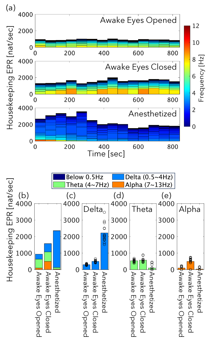
Figure 3: The contributions of each frequency band to the housekeeping entropy production rate (EPR) were stable across time windows compared to the differences across conditions. (a) $\sigma_{t}^{\mathrm{hk}(k)}$ from each 60 second time window are shown. The color indicates the frequency $\chi_{k}$. (b-e) The contribution to the housekeeping entropy production rate from the delta band $\sigma_{t}^{\mathrm{hk,Delta}}$, the theta band $\sigma_{t}^{\mathrm{hk,Theta}}$ and the alpha band $\sigma_{t}^{\mathrm{hk,Alpha}}$ [Eqs. (82), (83), and (84)] are shown. Stacked bar plots of all frequency bands are shown in (b). The displayed values are the averages over time windows. In (c-e), the contributions to the housekeeping entropy production rate from (c) the delta band $\sigma_{t}^{\mathrm{hk,Delta}}$, (d) the theta band $\sigma_{t}^{\mathrm{hk,Theta}}$, and (e) the alpha band $\sigma_{t}^{\mathrm{hk,Alpha}}$ are respectively shown. The bar plots represent the averaged values over time windows. Each circle represents the value of each time window.

To assess whether the degree of temporal variation in each frequency’s contribution to the housekeeping entropy production rate is small enough to detect the difference in each frequency’s contribution across conditions, we binned the oscillatory modes into the delta band (0.5-4Hz), the theta band (4-7Hz), alpha band (7-13Hz) and the frequency band below 0.5Hz according to the conventional definition of frequency bands in the brain [53] (Fig. 3b). The sums of the contributions from each frequency band are are summarized as $\sigma_{t}^{\mathrm{hk,<0.5}}$, $\sigma_{t}^{\mathrm{hk,Delta}}$, $\sigma_{t}^{\mathrm{hk,Theta}}$ and $\sigma_{t}^{\mathrm{hk,Alpha}}$ [Eqs. (81), (82), (83), and (84); see Methods section]. The sums of the contributions from each frequency band $\sigma_{t}^{\mathrm{hk,<0.5}}$, $\sigma_{t}^{\mathrm{hk,Delta}}$, $\sigma_{t}^{\mathrm{hk,Theta}}$, and $\sigma_{t}^{\mathrm{hk,Alpha}}$ calculated from each time window are shown in dot plots, and their averages across time windows are shown in bar plots (Fig. 3c-e). The plots show that the contributions to the housekeeping entropy production rate from each frequency band $\sigma_{t}^{\mathrm{hk,Delta}}$, $\sigma_{t}^{\mathrm{hk,Theta}}$, and $\sigma_{t}^{\mathrm{hk,Alpha}}$ differed across conditions. In this single monkey, we observed that contributions of the delta band $\sigma_{t}^{\mathrm{hk,Delta}}$ were larger in the anesthetized condition than in the awake conditions, contributions of the theta band $\sigma_{t}^{\mathrm{hk,Theta}}$ were larger in the awake conditions than in the anesthetized condition, and contributions of the alpha band $\sigma_{t}^{\mathrm{hk,Alpha}}$ were larger in the awake eyes closed condition than in the awake eyes open condition and in the anesthetized condition. From the dot plots in Figs. 3c-e, we can see that the time variations of $\sigma_{t}^{\mathrm{hk,Delta}}$, $\sigma_{t}^{\mathrm{hk,Theta}}$, and $\sigma_{t}^{\mathrm{hk,Alpha}}$ were smaller than the differences of $\sigma_{t}^{\mathrm{hk,Delta}}$, $\sigma_{t}^{\mathrm{hk,Theta}}$, and $\sigma_{t}^{\mathrm{hk,Alpha}}$ across the conditions. For the other monkeys, we also found that there are similar trends in the differences of $\sigma_{t}^{\mathrm{hk,Delta}}$ and $\sigma_{t}^{\mathrm{hk,Theta}}$ across the conditions, and that the temporal variations are smaller than these differences across the conditions, i.e., the decomposition is temporally stable (Fig. S1).

Furthermore, we found that the spatial distributions of the contributions to the entropy production rate from each frequency band were also stable across time windows (Fig. 4). The spatial distributions of the contributions to the entropy production rate from each frequency band are defined as the sums of $\bm{\sigma}_{t}^{\mathrm{hk}(k)}$ within each frequency band, as $\bm{\sigma}_{t}^{\mathrm{hk,Delta}}$, $\bm{\sigma}_{t}^{\mathrm{hk,Theta}}$, and $\bm{\sigma}_{t}^{\mathrm{hk,Alpha}}$ [Eqs. (86), (87), and (88); see Methods section]. Figure 4a-c shows the spatial distributions $\bm{\sigma}_{t}^{\mathrm{hk,Delta}}$, $\bm{\sigma}_{t}^{\mathrm{hk,Theta}}$, and $\bm{\sigma}_{t}^{\mathrm{hk,Alpha}}$ from four example time windows. We observed that the spatial distributions $\bm{\sigma}_{t}^{\mathrm{hk,Delta}}$, $\bm{\sigma}_{t}^{\mathrm{hk,Theta}}$, and $\bm{\sigma}_{t}^{\mathrm{hk,Alpha}}$ were stable over time under all conditions.

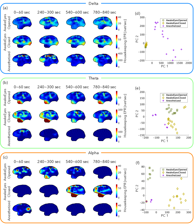
Figure 4: The spatial distributions of contributions from each frequency band to the housekeeping entropy production rate were stable across time windows compared to the differences across conditions. (a-c) The spatial distributions of contributions to the housekeeping entropy production rate from (a) the delta band $\bm{\sigma}_{t}^{\mathrm{hk,Delta}}$, (b) the theta band $\bm{\sigma}_{t}^{\mathrm{hk,Theta}}$, and (c) the alpha band $\bm{\sigma}_{t}^{\mathrm{hk,Alpha}}$ from four example time windows [Eqs. (86), (87), and (88)]. Note that for frequency bands that were not detected as an eigenvalue $\lambda_{k}$ of the matrix $\mathit{D}_{t}A_{t}^{\mathrm{hk}}$, zero values were plotted (the blue color was uniformly plotted) because the contributions of such components were 0. The quantities $\bm{\sigma}_{t}^{\mathrm{hk,Delta}}$, $\bm{\sigma}_{t}^{\mathrm{hk,Theta}}$, and $\bm{\sigma}_{t}^{\mathrm{hk,Alpha}}$ are represented by the colors at the location of each electrode. Each plot shows the brain viewed from the lateral side. (d-f) The spatial distributions of the contributions to the housekeeping entropy production rate from (d) the delta band $\bm{\sigma}_{t}^{\mathrm{hk,Delta}}$, (e) the theta band $\bm{\sigma}_{t}^{\mathrm{hk,Theta}}$, and (f) the alpha band $\bm{\sigma}_{t}^{\mathrm{hk,Alpha}}$ were visualized by projecting them onto two dimensions using principal component analysis. In the scatter plots, each point corresponds to the spatial distribution from each time window, projected onto two principal component spaces.

To assess whether the degree of temporal variation in the spatial distribution is small enough to detect the difference of the spatial distribution across conditions, the vectors of the spatial distributions of the contributions from each frequency band $\bm{\sigma}_{t}^{\mathrm{hk,Delta}}$, $\bm{\sigma}_{t}^{\mathrm{hk,Theta}}$, and $\bm{\sigma}_{t}^{\mathrm{hk,Alpha}}$, whose dimension is the number of electrodes, were visualized by projecting them onto two dimensions using principal component analysis (Fig. 4d-f). In the scatter plots, each point corresponds to the spatial distribution from each time window, projected onto two principal component spaces. In the delta band, points corresponding to the awake eyes opened and awake eyes closed conditions are plotted at closer positions, while those corresponding to the anesthetized condition are plotted at more distant positions. For the theta and alpha bands, points are plotted in separate positions for each condition. In all instances, the plots show that the variations between time windows are smaller than the differences across conditions. Note that for frequency bands not detected as an eigenvalue $\lambda_{k}$ of the matrix $\mathit{D}_{t}A_{t}^{\mathrm{hk}}$, zero values are plotted in Fig. 4a-c, as observed in the plot for the alpha waves under anesthetic conditions, for instance. Such oscillation modes are projected to the same point, as can be seen at the bottom right of Fig. 4f.

VI.3 Comparison of the results of our decomposition across conditions

Having confirmed that the contributions from each frequency band $\sigma_{t}^{\mathrm{hk,Delta}}$, $\sigma_{t}^{\mathrm{hk,Theta}}$, and $\sigma_{t}^{\mathrm{hk,Alpha}}$ were stable over time (Figs. 3 and 4), we investigated whether there were consistent features of the decomposition for different conditions across multiple monkeys with multiple recording sessions. Figure 5 summarizes the results of decomposition across individual monkeys and recording sessions. For each monkey and session, we computed the z-scores of $\sigma_{t}^{\mathrm{hk,Delta}}$, $\sigma_{t}^{\mathrm{hk,Theta}}$, and $\sigma_{t}^{\mathrm{hk,Alpha}}$ and compared them across conditions (Fig. 5a). We calculated their z-scores of them across all time windows and conditions independently for each monkey, recording session, and frequency band. For the details on the calculation of the z-scores, see the Methods section. We also calculated the the z-scores of $\sigma_{t}^{\mathrm{hk}}$ across all time windows and conditions independently for each monkey, recording session (Fig. 5b).

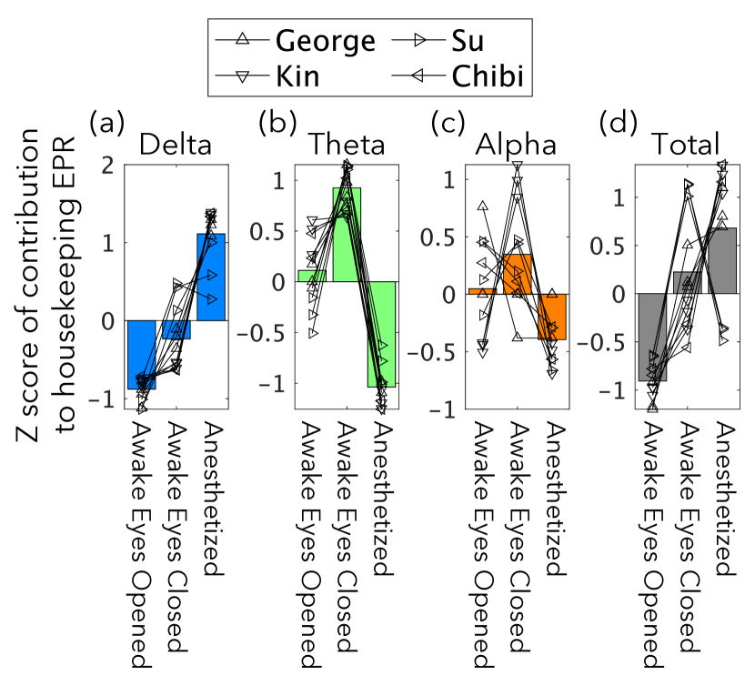
Figure 5: Difference in the contribution of each frequency band to the housekeeping entropy production rate (EPR) between different conditions for all monkeys and recording sessions. (a-c) The plots show the z-scores of the contribution to the housekeeping EPR from (a) the alpha band $\sigma_{t}^{\mathrm{hk,Delta}}$, (b) the theta band $\sigma_{t}^{\mathrm{hk,Theta}}$, and (c) the alpha band $\sigma_{t}^{\mathrm{hk,Alpha}}$. Each dot represents z-scores calculated in a single recording session from a single monkey. The displayed values are the averages of the z-scores across time windows within each condition. In the plot, results from the same recording session from the same monkey are connected by lines, and markers represent individual monkeys (George, Su, Kin and Chibi). Bar plots show the average across monkeys and recording sessions. (d) The z-scores of the housekeeping EPR $\sigma_{t}^{\mathrm{hk}}$ are shown in similar way to (a-c).

We observed several robust tendencies across all individual monkeys that (i) the contributions of the delta band were larger in the anesthetized condition than in the awake conditions (Fig. 5a), (ii) the contributions of theta band were smaller in the anesthetized condition than in the awake conditions (Fig. 5b), (iii) the contributions of alpha band were larger in the awake eyes open condition than in the anesthetized condition (Fig. 5c). In addition, we observed a modest tendency in 3 out of 4 individual monkeys (vi) that the z-values of the total $\sigma_{t}^{\mathrm{hk}}$ were larger in the anesthetized condition than in the awake conditions (Fig. 5d).

VII Discussion

In this paper, we derived a relationship between oscillations and the entropy production rate. The housekeeping entropy production rate can be simultaneously decomposed into contributions from each oscillatory mode and each dimension $\sigma_{t}^{\mathrm{hk}(k,i)}$ [Eq. (68)]. Oscillatory modes with larger normalized intensity $J_{k}$ or frequency $\chi_{k}$ have a larger contribution to the housekeeping entropy production rate. Furthermore, when applied to neural activity data recorded using ECoG [42], it is observed that contributions from each frequency band remain stable. Under anesthetized conditions, compared to the awake conditions, the contributions from the delta wave (0.5-4Hz) were larger, while those from the theta wave (4-7Hz) were smaller. Since the entropy production rate determines various limits of information processing [19, 27, 29, 25], these results might lead to a better understanding of the role of oscillations in brain information processing.

VII.1 Significance of decomposing EPR to oscillatory contributions

First, we discuss relationships between our decomposition and other methods for extracting oscillatory components, such as the Fourier transform and dynamic mode decomposition (DMD) [54, 55]. The Fourier transform is a commonly used method in neuroscience that extracts all frequency components below the Nyquist frequency for each electrode. However, the Fourier transform has limitations: (i) it extracts all frequencies indiscriminately, potentially leading to statistical overfitting, and (ii) it does not capture the oscillatory patterns across multiple electrodes. DMD addresses these issues by decomposing the multivariate time series of $\bm{x}$ into a small number of spatio-temporal oscillatory modes through the eigenvalue decomposition of auto-regressive coefficients. The spatio-temporal oscillatory modes obtained in our decomposition in Eq. (47) are similar to the oscillatory modes obtained in DMD. The important and distinctive feature is that our decomposition provides the therodynamic meaning for such DMD-like oscillatory modes by elucidating the contributions of each oscillatory mode to the entropy production rate, which we believe is useful for understanding the nature of information processing in the brain.

Specifically, the entropy production rate has a utility to determine various physical limits of information processing, including limits of speed [22, 24, 25, 26] and accuracy [27, 20, 28] of the information processing. For the potential applications in neuroscience, these relations allow us to quantify, for example, (i) the limits of information processing in the brain, or (ii) how close the brain’s information processing is to the physical limits. Such quantifications could provide a mathematical framework to capture, for example, the brain development and learning. In such applications, our decomposition may explain previous reports of changes in neural oscillations, such as delta and beta waves, associated with development [56, 57] or learning [58, 59]. As another example, a previous study has computed the entropy production rate and discussed the relationships to cognitive cost  [37]. Our decomposition may be useful for further interpreting the relationships between cognitive cost and the entropy production rate in terms of oscillations.

We also note its applicability to other systems. Regarding the fluctuation-response relation violation, the heat for Langevin systems can be decomposed via the Fourier transform [60]. In the steady state, the entropy production rate is given by the heat, and the result in Ref. [60] can be generalized for the entropy production rate. Specifically, such a decomposition of the entropy production rate has been discussed to analyze the spatiotemporal dissipation for the active matter [61] and nonequilibrium crystals [62]. Thus, our DMD-like decomposition may provide a complementary method to analyze the spatiotemporal dissipation for other systems, such as the active matter and nonequilibrium crystals. A relation between our DMD-like decomposition and a geometric decomposition via the spatial Fourier transform [63] is also interesting.

VII.2 Interpretation of the macroscopic entropy production rate calculated from ECoG recording

Here we discuss the interpretations of the entropy production rate calculated from the ECoG recordings, which are macroscopic observations of neural activity. The entropy production rate quantified at the macroscopic scale is different from its microscopic counterpart in thermodynamics and it may not determine the limits of information processing at the microscopic level of brain activity, although the macroscopic entropy production rate is known to be a lower bound of the microscopic entropy production rate [64]. An important point is that the entropy production rate calculated from ECoG data has its own meaning because it provides the limit of information processing at the similar macroscopic scale, although not necessarily at the microscopic level of brain activity. Neuroscience research has found various insights at this macroscopic level, extracting information related to visual [65] or auditory experiences [66], working memory [67], motor movements [68], and intentions [69]. The application of stochastic thermodynamics to these domains opens avenues for investigating how the macroscopic entropy production rate influences the thermodynamic constraints on the speed and precision of information processing. Our theoretical results [Eq. (68)] also allow the exploration of this concept in the context of neural oscillation.

VII.3 Findings about brain dynamics from the biological or clinical perspective

In this section, we discuss the biological or clinical implications of the ECoG data analysis. First, we found that large entropy production rate occurs even during the anesthetized state. Anesthesia is known to reduce the activation level [70] or glucose consumption [71] in the brain compared to the awake state. One might intuitively assume that the entropy production rate at the macroscopic scale (at the scale of the ECoG signals) would also be small. However, our results showed that in the anesthetized state, the entropy production rate originating mainly from the high-intensitiy delta-band wave was very large, which was comparable to the total entropy production rate in the awake state. Although the slow frequency band, such as the delta band, contributes less to the entropy production rate than the higher frequency band according to our theoretical results, it generates very large entropy production rate due to its high intensity. This seemingly counterintuive result that anesthesia would cause large entropy production rate to maintain a low frequency but high intensity wave, would shed new light on the biological or clinical consequences of the anesthesia.

On the other hand, during the awake state, the entropy production rate is consumed by the generation of faster oscillations, such as theta and alpha waves, while the contribution of the delta wave is much lower than in the anesthetized state. Although we did not observe higher frequency oscillations, such as beta waves (13-30Hz) or gamma waves (30-70Hz), we speculate that the entropy production rates in these frequencies are generated as needed, depending on the task demands, because it is known that these frequencies are enhanced only during specific cognitive tasks such as motor control or visual processing.

Taken together, by using our decomposition, we found for the first time that both the awake and anesthetized states generate a comparable amount of entropy production rate but the origin of the entropy production rate, i.e., how the entropy production rate is generated from the characteristic of dynamical systems, is drastically different between the anesthetized and awake states. In the anesthetized state, the entropy production rate is caused by slow and high intensity oscillations, whereas in the awake state, it is caused by faster and lower intensity oscillations.

This difference in the origins of the entropy production rate between the awake and anesthetized states would also imply that the neural mechanisms generating the entropy production rate are different. In fact, it is known that the delta wave, the theta wave, and the alpha wave are generated by different neural mechanisms: the delta wave wave arises from the interaction of neurons within the thalamocortical circuit [43, 1], the theta wave arises from the population activity within the hippocampus [1, 72], and the alpha wave arise from the supragranular layers of the cortex and propagate from higher areas to lower areas and the thalamus [73]. Although it is impossible to investigate these circuits involving deep brain regions using ECoG data that is placed on the surface of the cortex, applying our decomposition to data in these circuits using deep recordings such as neuropixels, will advance our understanding of thermodynamic dissipation and the neural substrates that cause it. Such an understanding cannot be achieved by simply computing the total entropy production rate without spatiotemporal decomposition.

In light of these findings, our study opens new avenues for clinical applications, particularly in the diagnosis and understanding of disorders of consciousness. Prior research, including studies using monkey ECoG [39] and human fMRI [38], has highlighted differences in entropy production rates across various states of consciousness, such as awake, anesthetized, and sleep states. Moreover, recent work has shown distinct patterns in the irreversibility of brain dynamics, which is closely tied to entropy production rate, between the awake state and various disordered states of consciousness, including minimally conscious states and unresponsive wakefulness syndrome [74]. Importantly, these disorders have also been associated with specific neural oscillation patterns [75, 76, 77]. By integrating our findings on the entropy production rate, particularly the differences in its origin and characteristics between awake and anesthetized states, with these previous studies, our decomposition approach offers a novel and comprehensive framework for the assessment of consciousness disorders. This framework, by simultaneously considering entropy production rates, oscillation patterns, and their spatial distribution, holds the potential to provide more nuanced and informative diagnostics compared to existing methods. Such advancements could significantly enhance our understanding and ability to effectively diagnose and treat disorders of consciousness.

VII.4 The difference of the entropy production rate between awake and anesthetized conditions

Our finding that the entropy production rate was higher under anesthetized conditions than under awake conditions in three out of four monkeys (Fig. 5d) may seem counterintuitive as discussed in the Section VII.3. Note, however, that this result does not necessarily mean that the anesthetized condition has a higher information processing performance in terms of speed or precision than the awake condition. This is because the entropy production rate relates only to the physical limits of information processing, not to the performance of the information processing itself. In our results, the higher entropy production rate in the anesthetized condition is due to the increase in delta-band activity (Fig. 5d), but it does not necessarily mean that the increase in delta-band activity contributes to a higher information processing performance.

On the other hand, a previous study that calculated the entropy production rate using the same ECoG data [39] shows different results from ours. It reported a lower entropy production rate in the anesthetized condition than in the awake eyes closed condition, while our results showed the opposite tendency in three out of four of monkeys (Fig. 5d). The discrepancy might be due to different statistical modeling. We treated the brain state as a real-valued vector $\bm{x}_{t}$ (a continuous state) and computed the entropy production rate by approximating the neural dynamics to a linear Gaussian process, while the previous study binned the low-dimensional brain state extracted by PCA into discrete states and computed the entropy production rate assuming a nonlinear process for the time series of these discrete states. While this approach can account for the nonlinearity of neural dynamics, it cannot capture high-dimensional dynamics and loses the spatial information of the ECoG electrodes.

In the future, it is desirable to extend our decomposition to handle nonlinear dynamics while preserving the high dimensionality and spatial information of the brain dynamics, and to compare these results with those obtained previously. We are currently working on extending our framework to nonlinear cases and will present the results elsewhere.

VIII Methods

VIII.1 Pre-processing

We applied the main result to neural data. We used a 128-channel ECoG dataset recorded from a monkey that is publicly available [42]. Data were recorded during awake eyes open, awake eyes closed, and ketamine-medetomidine-induced anesthesia.

The data are pre-processed in the following steps. The data, originally sampled at 1000 Hz, were downsampled to 200 Hz using the pop_resample function from EEGLAB [78], with a cutoff frequency of 80 Hz and a transition bandwidth of 40 Hz. This was followed by a high pass filter applied at 2 Hz using the pop_eegfiltnew function from EEGLAB [78] to remove trend components and increase data stationarity. Line noise at 50 Hz and 100 Hz was then removed using EEGLAB’s cleanline function. To assess electrode quality, the standard deviation over time was calculated for each electrode. Electrodes with a standard deviation greater than three times the median standard deviation across all electrodes were considered poor and were subsequently removed. Finally, the data were rereferenced using a bipolar scheme. The downsampling and high-pass filter frequencies were chosen to avoid the artifacts described in Ref. [79], following the instructions of Ref. [80].

VIII.2 Model fitting

The pre-processed data are fitted to the Langevin equation [Eq. (20)]. The equation to be fit is

$$d\bm{x}_{t}=\mathit{D}\mathit{A}\bm{x}_{t}dt+\sqrt{2}\mathit{G}d\bm{B}_{t}$$ (74)

under the following assumptions. To plot the contribution of each electrode’s oscillation to the housekeeping entropy production rate using Eq. (60), we assume that the noise coefficient $\mathit{G}_{t}$ is a diagonal matrix. In addition, the data were divided into 60-second time windows, and assumed to be stationary within each time window. Furthermore, within these time windows, both $\mathit{A}_{t},\bm{b},\mathit{D}_{t}$ and $\mathit{G}_{t}$ are assumed to be time invariant, hence denoted as $\mathit{A},\bm{b},\mathit{D}$ and $\mathit{G}$ respectively. Furthermore, the mean over time was subtracted from the data, so that the mean of the data $\bm{\mu}_{t}$, is equal to the zero vector. This procedure makes $\bm{b}$ be the zero vector based on Eq. (23).

The matrices $\mathit{D}\mathit{A}$ and $\mathit{D}$ were estimated by maximum likelihood estimation. The differential $d\bm{x}_{t}$ was approximated by the difference of the measured data for one time step. Since the sampling rate of the preprocessed data was 200Hz, one time step corresponds to $dt=0.005$ seconds. The analytic expressions for the estimators of the matrix $\widehat{\mathit{DA}}$ and the diagonal elements of the matrix $2\widehat{\mathit{D}}$ are

$$\widehat{\mathit{DA}}dt =\quantity(\sum_{t=1}^{N-1}d\bm{x}_{t}\bm{x}_{t}^{\top})\quantity(\sum_{t=1}^{N-1}\bm{x}_{t}\bm{x}_{t}^{\top})^{-1},$$ (75)

$$2\widehat{D}_{ii}dt =\frac{1}{N-1}\sum_{t=1}^{N-1}\quantity(dx_{t}^{(i)}-\quantity(\widehat{\mathit{DA}})_{i:}\bm{x}_{t}dt)^{2},$$ (76)

where $N$ is the number of time steps of the data, $dx_{t}^{(i)}$ is the $i$-th component of $d\bm{x}_{t}$, and $(\widehat{\mathit{DA}})_{i:}$ is the $i$-th row vector of the matrix $\widehat{\mathit{DA}}$. The symbol $\widehat{\ }$ represents an estimator and is used to distinguish it from the true value. Note that $\widehat{\mathit{D}}$ is a diagonal matrix, since the noise coefficient $G$ is assumed to be a diagonal matrix. Using these estimators, the estimator of the matrix $\widehat{\mathit{A}}$ is given as

$$\widehat{\mathit{A}}=\widehat{\mathit{D}}^{-1}\widehat{\mathit{DA}}.$$ (77)

To satisfy the stationarity assumption under the estimated values of $\widehat{\mathit{DA}}$ and $\widehat{\mathit{D}}$ as described above, the covariance matrix $\widehat{\mathit{\Sigma}}$ was estimated as follows:

$$\widehat{\mathit{\Sigma}}=-\sum_{k,l}\frac{1}{\kappa_{k}+\overline{\kappa}_{l}}\mathsf{H}_{k}(2\widehat{D})\mathsf{H}_{l}^{*},$$ (78)

where $\kappa_{k}$ is the $k$-th eigenvalue of $\widehat{\mathit{DA}}$ and $\mathsf{H}_{k}$ is the projection matrix that provides the spectoral decomposition of $\widehat{\mathit{DA}}$ as $\widehat{\mathit{DA}}=\sum_{k}\kappa_{k}\mathsf{H}_{k}$. This $\widehat{\mathit{\Sigma}}$ satisfies the condition of stationarity $\dot{\mathit{\Sigma}}=0$ in the Lyapunov equation (24) because the projection matrix satisfies $\sum_{k}\mathsf{H}_{k}=I$ and $\mathsf{H}_{k}\mathsf{H}_{j}=\delta_{kj}\mathsf{H}_{k}$.

The excess part $\widehat{\mathit{A}^{\mathrm{ex}}}$ and the housekeeping part $\widehat{\mathit{A}^{\mathrm{hk}}}$ of $\widehat{\mathit{A}}$ are given as follows. Since we assumed $\widehat{\mathit{A}}$ and $\widehat{\mathit{\Sigma}}$ to be time-invariant, we omitted the subscript $t$ from $\widehat{\mathit{A}_{t}^{\mathrm{ex}}}$ and $\widehat{\mathit{A}_{t}^{\mathrm{hk}}}$. Since $\widehat{\mathit{A}^{\mathrm{ex}}}$ is a unique symmetry matrix satisfying (30), we can write

$$\widehat{\mathit{A}^{\mathrm{ex}}}=-\widehat{\mathit{\Sigma}}^{-1},$$ (79)

under the assumption that $\dot{\mathit{\Sigma}}=0$. Using $\widehat{\mathit{A}}$ in equation (75) and $\widehat{\mathit{A}^{\mathrm{ex}}}$ in equation (79), we get

$$\widehat{\mathit{DA}^{\mathrm{hk}}}=\widehat{\mathit{DA}}-\widehat{\mathit{D}}\widehat{\mathit{A}^{\mathrm{ex}}}.$$ (80)

The spectral decomposition of $\widehat{\mathit{DA}^{\mathrm{hk}}}$ (Eq. 49) allows us to apply our decomposition of the housekeeping entropy production rate into oscillatory components (Eq. 60) to data analysis.

VIII.3 Visualization of Results

In Figs. 3 and 5, the contributions of each oscillatory mode $\sigma_{t}^{\mathrm{hk,(k)}}$ are binned into the delta band (0.5-4Hz), theta band (4-7Hz), alpha band (7-13Hz), and the frequency band below 0. 5Hz, according to the conventional definition of frequency bands in the brain [2, 3, 4, 5, 6, 7, 8, 9]. The sums of the contributions from each frequency band are summarized as $\sigma_{t}^{\mathrm{hk,<0.5}}$, $\sigma_{t}^{\mathrm{hk,Delta}}$, $\sigma_{t}^{\mathrm{hk,Theta}}$, and $\sigma_{t}^{\mathrm{hk,Alpha}}$. They are defined as

$$\sigma_{t}^{\mathrm{hk,<0.5}} =\sum_{k|0\leq|\chi_{k}|\leq 0.5}\sigma_{t}^{\mathrm{hk}(k)}$$ (81)

$$\sigma_{t}^{\mathrm{hk,Delta}} =\sum_{k|0.5\leq|\chi_{k}|\leq 4}\sigma_{t}^{\mathrm{hk}(k)}$$ (82)

$$\sigma_{t}^{\mathrm{hk,Theta}} =\sum_{k|4\leq|\chi_{k}|\leq 7}\sigma_{t}^{\mathrm{hk}(k)}$$ (83)

$$\sigma_{t}^{\mathrm{hk,Alpha}} =\sum_{k|7\leq|\chi_{k}|\leq 13}\sigma_{t}^{\mathrm{hk}(k)}.$$ (84)

In Fig. 4, the spatial distributions of the contributions to the entropy production rate from each frequency band $\bm{\sigma}_{t}^{\mathrm{hk,<0.5}}$, $\bm{\sigma}_{t}^{\mathrm{hk,Delta}}$, $\bm{\sigma}_{t}^{\mathrm{hk,Theta}}$, and $\bm{\sigma}_{t}^{\mathrm{hk,Alpha}}$ were shown. They are defined as

$$\bm{\sigma}_{t}^{\mathrm{hk,<0.5}} =(\sigma_{t}^{\mathrm{hk,<0.5},(i=1)},\cdots,\sigma_{t}^{\mathrm{hk,<0.5},(i=d)})$$ (85)

$$\bm{\sigma}_{t}^{\mathrm{hk,Delta}} =(\sigma_{t}^{\mathrm{hk,Delta},(i=1)},\cdots,\sigma_{t}^{\mathrm{hk,Delta},(i=d)})$$ (86)

$$\bm{\sigma}_{t}^{\mathrm{hk,Theta}} =(\sigma_{t}^{\mathrm{hk,Theta},(i=1)},\cdots,\sigma_{t}^{\mathrm{hk,Theta},(i=d)})$$ (87)

$$\bm{\sigma}_{t}^{\mathrm{hk,Alpha}} =(\sigma_{t}^{\mathrm{hk,Alpha},(i=1)},\cdots,\sigma_{t}^{\mathrm{hk,Alpha},(i=d)}),$$ (88)

where

$$\sigma_{t}^{\mathrm{hk,<0.5},(i)} =\sum_{k|0\leq|\chi_{k}|\leq 0.5}\sigma_{t}^{\mathrm{hk}(k,i)}$$ (89)

$$\sigma_{t}^{\mathrm{hk,Delta},(i)} =\sum_{k|0.5\leq|\chi_{k}|\leq 4}\sigma_{t}^{\mathrm{hk}(k,i)}$$ (90)

$$\sigma_{t}^{\mathrm{hk,Theta},(i)} =\sum_{k|4\leq|\chi_{k}|\leq 7}\sigma_{t}^{\mathrm{hk}(k,i)}$$ (91)

$$\sigma_{t}^{\mathrm{hk,Alpha},(i)} =\sum_{k|7\leq|\chi_{k}|\leq 13}\sigma_{t}^{\mathrm{hk}(k,i)}.$$ (92)

Appendix A Detailed derivation of Eq. (5)

To derive Eq. (5), we start with the following expression,

$$\mathrm{D_{KL}}[\mathbb{P}_{\rm F}\|\mathbb{P}_{\rm B}]$$

$$= \int d\bm{x}_{t}d\bm{x}_{t+dt}\mathbb{P}_{\rm F}(\bm{x}_{t+dt},\bm{x}_{t})\ln\frac{\mathbb{T}(\bm{x}_{t+dt}|\bm{x}_{t})p_{t}(\bm{x}_{t})}{\mathbb{T}(\bm{x}_{t}|\bm{x}_{t+dt})p_{t+dt}(\bm{x}_{t+dt})}$$

$$= \int d\bm{x}_{t}d\bm{x}_{t+dt}\mathbb{P}_{\rm F}(\bm{x}_{t+dt},\bm{x}_{t})\ln\frac{\mathbb{T}(\bm{x}_{t+dt}|\bm{x}_{t})p_{t}(\bm{x}_{t})}{\mathbb{T}(\bm{x}_{t}|\bm{x}_{t+dt})p_{t}(\bm{x}_{t+dt})}$$

$$+\int d\bm{x}_{t+dt}p_{t+dt}(\bm{x}_{t+dt})\ln\frac{p_{t}(\bm{x}_{t+dt})}{p_{t+dt}(\bm{x}_{t+dt})},$$ (93)

where we used the fact $\int d\bm{x}_{t}\mathbb{P}_{\rm F}(\bm{x}_{t+dt},\bm{x}_{t})=p_{t+dt}(\bm{x}_{t+dt})$. Here, the last term

$$\int d\bm{x}_{t+dt}p_{t+dt}(\bm{x}_{t+dt})\ln\frac{p_{t}(\bm{x}_{t+dt})}{p_{t+dt}(\bm{x}_{t+dt})}=O(dt^{2}),$$ (94)

is negligible. By using the transition probability Eq. (8), we can calculate the quantity $\ln[\mathbb{T}(\bm{x}_{t+dt}|\bm{x}_{t})p_{t}(\bm{x}_{t})]/[\mathbb{T}(\bm{x}_{t}|\bm{x}_{t+dt})p_{t}(\bm{x}_{t+dt})]$ as

$$\ln\frac{\mathbb{T}(\bm{x}_{t+dt}|\bm{x}_{t})p_{t}(\bm{x}_{t})}{\mathbb{T}(\bm{x}_{t}|\bm{x}_{t+dt})p_{t}(\bm{x}_{t+dt})}$$

$$= \frac{(\dot{\bm{x}}_{t})^{\top}(\bm{f}_{t}(\bm{x}_{t})+\bm{f}_{t}(\bm{x}_{t+dt}))dt}{2}$$

$$-\frac{(\dot{\bm{x}}_{t})^{\top}[\nabla\ln p_{t}(\bm{x}_{t})+\nabla\ln p_{t}(\bm{x}_{t+dt})]}{2}+C$$

$$= D^{-1}_{t}\bm{\nu}_{t}(\bm{x}_{t})\circ\dot{\bm{x}}_{t}dt+C,$$ (95)

where $\circ$ stands for Stratonovich integral which is defined as $\bm{y}(\bm{x}_{t})\circ\dot{\bm{x}}_{t}=(\bm{x}_{t+dt}-\bm{x}_{t})^{\top}[\bm{y}(\bm{x}_{t})+\bm{y}(\bm{x}_{t+dt})]/(2dt)$ for any vector $\bm{y}(\bm{x}_{t})$, and $C$ is the negligible term that satisfies $\int d\bm{x}_{t}d\bm{x}_{t+dt}\mathbb{P}_{\rm F}(\bm{x}_{t+dt},\bm{x}_{t})C=O(dt^{2})$. By neglecting $O(dt^{2})$, the Kullback–Leibler divergence is calculated as

$$\mathrm{D_{KL}}[\mathbb{P}_{\rm F}\|\mathbb{P}_{\rm B}]$$

$$=\int d\bm{x}_{t}d\bm{x}_{t+dt}\mathbb{T}(\bm{x}_{t+dt}|\bm{x}_{t})p_{t}(\bm{x}_{t})D^{-1}_{t}\bm{\nu}_{t}(\bm{x}_{t})\circ\dot{\bm{x}}_{t}dt.$$ (96)

To obtain Eq. (5) from the expression in Eq. (96), we consider the following formula

$$\int d\bm{x}_{t}d\bm{x}_{t+dt}\mathbb{T}(\bm{x}_{t+dt}|\bm{x}_{t})p_{t}(\bm{x}_{t})\bm{y}(\bm{x}_{t})\circ\dot{\bm{x}}_{t}dt$$

$$=\int d\bm{x}_{t}p_{t}(\bm{x}_{t})(\bm{y}(\bm{x}_{t}))^{\top}\bm{\nu}_{t}(\bm{x}_{t})dt,$$ (97)

for any vector $\bm{y}(\bm{x}_{t})$. To prove it, we start with the following Gaussian integral,

$$\int d\bm{x}_{t+dt}\mathbb{T}(\bm{x}_{t+dt}|\bm{x}_{t})\bm{y}(\bm{x}_{t})\circ d\bm{x}_{t}dt$$

$$= \int d\bm{x}_{t}\mathbb{T}(\bm{x}_{t+dt}|\bm{x}_{t})\left[\frac{\bm{y}(\bm{x}_{t})+\bm{y}(\bm{x}_{t+dt})}{2}\right]^{\top}(\bm{x}_{t+dt}-\bm{x}_{t})$$

$$= \int d\bm{x}_{t}\mathbb{T}(\bm{x}_{t+dt}|\bm{x}_{t})[\bm{y}(\bm{x}_{t})]^{\top}(\bm{x}_{t+dt}-\bm{x}_{t})$$

$$+\sum_{i,j}\int d\bm{x}_{t}\mathbb{T}(\bm{x}_{t+dt}|\bm{x}_{t})$$

$$\>\>\>\times\frac{[(\nabla)_{j}(\bm{y}(\bm{x}_{t}))_{i}](\bm{x}_{t+dt}-\bm{x}_{t})_{i}(\bm{x}_{t+dt}-\bm{x}_{t})_{j}}{2}$$

$$= [\bm{y}(\bm{x}_{t})]^{\top}D_{t}\bm{f}_{t}(\bm{x}_{t})dt+\sum_{i,j}[(\nabla)_{j}(\bm{y}(\bm{x}_{t}))_{i}](D_{t})_{ij}dt$$ (98)

where we neglect the higher order term $O(dt^{2})$. Thus, we obtain the formula as follows,

$$\int d\bm{x}_{t}d\bm{x}_{t+dt}\mathbb{T}(\bm{x}_{t+dt}|\bm{x}_{t})p_{t}(\bm{x}_{t})\bm{y}(\bm{x}_{t})\circ d\bm{x}_{t}dt$$

$$= \int d\bm{x}_{t}p_{t}(\bm{x}_{t})[\bm{y}(\bm{x}_{t})]^{\top}D_{t}\bm{f}_{t}(\bm{x}_{t})dt$$

$$+\sum_{i,j}\int d\bm{x}_{t}p_{t}(\bm{x}_{t})[(\nabla)_{j}(\bm{y}(\bm{x}_{t}))_{i}](D_{t})_{ij}dt$$

$$= \int d\bm{x}_{t}p_{t}(\bm{x}_{t})[\bm{y}(\bm{x}_{t})]^{\top}D_{t}\bm{f}_{t}(\bm{x}_{t})dt$$

$$-\int d\bm{x}_{t}p_{t}(\bm{x}_{t})[\bm{y}(\bm{x}_{t})]^{\top}D_{t}\nabla\ln p_{t}(\bm{x}_{t})dt$$

$$= \int d\bm{x}_{t}p_{t}(\bm{x}_{t})(\bm{y}(\bm{x}_{t}))^{\top}\bm{\nu}_{t}(\bm{x}_{t})dt,$$ (99)

where we used the partial integration with the assumption that $p_{t}(\bm{x}_{t})\to 0$ in the limit $\|\bm{x}_{t}\|\to\infty$.

By using the formula Eq. (97) for $\bm{y}(\bm{x}_{t})=D_{t}^{-1}\bm{\nu}_{t}(\bm{x}_{t})$, we can obtain Eq. (5) from the expression in Eq. (96),

$$\mathrm{D_{KL}}[\mathbb{P}_{\rm F}\|\mathbb{P}_{\rm B}] =\int d\bm{x}_{t}p_{t}(\bm{x}_{t})(D^{-1}_{t}\bm{\nu}_{t}(\bm{x}_{t}))^{\top}\bm{\nu}_{t}(\bm{x}_{t})dt$$

$$=\sigma_{t}dt.$$ (100)

Appendix B Robustness of temporal stability of the decomposition across all individual monkeys

The temporal stability of the decomposition was robust across all individual monkeys. Similar to the Fig. 3b-e, the sums of the contributions from each frequency band $\sigma_{t}^{\mathrm{hk,<0.5}}$, $\sigma_{t}^{\mathrm{hk,Delta}}$, $\sigma_{t}^{\mathrm{hk,Theta}}$, and $\sigma_{t}^{\mathrm{hk,Alpha}}$ calculated from each time window are shown in the dot plots, and their averages across time windows are shown in the bar plots (Fig. S1). For all individual monkeys, we observed that the contributions of the delta band $\sigma_{t}^{\mathrm{hk,Delta}}$ were larger in the anesthetized condition than in the awake conditions, and the contributions of the theta band $\sigma_{t}^{\mathrm{hk,Theta}}$ were larger in the awake conditions than in the anesthetized condition. The dot plots in Fig. S1 show that the time variations of $\sigma_{t}^{\mathrm{hk,Delta}}$ and $\sigma_{t}^{\mathrm{hk,Theta}}$ were smaller than these differences across conditions.

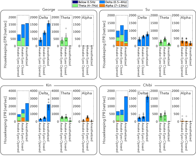
Figure S1: The temporal stability of the contributions of each frequency band to the housekeeping entropy production rate (EPR) was robust across all individual monkeys (George, Su, Kin and Chibi). The contribution to the housekeeping entropy production rate from the delta band $\sigma_{t}^{\mathrm{hk,Delta}}$, the theta band $\sigma_{t}^{\mathrm{hk,Theta}}$ and the alpha band $\sigma_{t}^{\mathrm{hk,Alpha}}$ [Eqs. (82), (83), and (84)] are shown. The displayed values are the averages over time windows. The contributions to the housekeeping entropy production rate from the delta band $\sigma_{t}^{\mathrm{hk,Delta}}$, the theta band $\sigma_{t}^{\mathrm{hk,Theta}}$, and the alpha band $\sigma_{t}^{\mathrm{hk,Alpha}}$ are respectively shown. The bar plots represent the averaged values over time windows. Each circle represents the value of each time window. The plots for Kin show the same figure as Fig. 3b-e.

References

• Buzsáki [2006] G. Buzsáki, Rhythms of the brain (2006).
• Clayton et al. [2018] M. S. Clayton, N. Yeung, and R. Cohen Kadosh, The many characters of visual alpha oscillations, Eur. J. Neurosci. 48, 2498 (2018).
• Jensen et al. [2014] O. Jensen, B. Gips, T. O. Bergmann, and M. Bonnefond, Temporal coding organized by coupled alpha and gamma oscillations prioritize visual processing, Trends Neurosci. 37, 357 (2014).
• Klimesch [2012] W. Klimesch, Alpha-band oscillations, attention, and controlled access to stored information, Trends Cogn. Sci. 16, 606 (2012).
• Foxe and Snyder [2011] J. J. Foxe and A. C. Snyder, The role of Alpha-Band brain oscillations as a sensory suppression mechanism during selective attention, Front. Psychol. 2, 154 (2011).
• Roux and Uhlhaas [2014] F. Roux and P. J. Uhlhaas, Working memory and neural oscillations: alpha–gamma versus theta–gamma codes for distinct WM information?, Trends Cogn. Sci. 18, 16 (2014).
• Sauseng et al. [2010] P. Sauseng, B. Griesmayr, R. Freunberger, and W. Klimesch, Control mechanisms in working memory: a possible function of EEG theta oscillations, Neurosci. Biobehav. Rev. 34, 1015 (2010).
• Engel and Fries [2010] A. K. Engel and P. Fries, Beta-band oscillations—signalling the status quo?, Curr. Opin. Neurobiol. 20, 156 (2010).
• Donoghue et al. [1998] J. P. Donoghue, J. N. Sanes, N. G. Hatsopoulos, and G. Gaál, Neural discharge and local field potential oscillations in primate motor cortex during voluntary movements, J. Neurophysiol. 79, 159 (1998).
• Jensen and Colgin [2007] O. Jensen and L. L. Colgin, Cross-frequency coupling between neuronal oscillations, Trends Cogn. Sci. 11, 267 (2007).
• Canolty and Knight [2010] R. T. Canolty and R. T. Knight, The functional role of cross-frequency coupling, Trends Cogn. Sci. 14, 506 (2010).
• Arnal et al. [2011] L. H. Arnal, V. Wyart, and A.-L. Giraud, Transitions in neural oscillations reflect prediction errors generated in audiovisual speech, Nat. Neurosci. 14, 797 (2011).
• Arnal and Giraud [2012] L. H. Arnal and A.-L. Giraud, Cortical oscillations and sensory predictions, Trends Cogn. Sci. 16, 390 (2012).
• Fries [2015] P. Fries, Rhythms for cognition: Communication through coherence, Neuron 88, 220 (2015).
• Womelsdorf et al. [2007] T. Womelsdorf, J.-M. Schoffelen, R. Oostenveld, W. Singer, R. Desimone, A. K. Engel, and P. Fries, Modulation of neuronal interactions through neuronal synchronization, Science 316, 1609 (2007).
• Sekimoto [2010] K. Sekimoto, Stochastic energetics (2010).
• Van den Broeck and Esposito [2010] C. Van den Broeck and M. Esposito, Three faces of the second law. ii. fokker-planck formulation, Physical Review E 82, 011144 (2010).
• Seifert [2012] U. Seifert, Stochastic thermodynamics, fluctuation theorems and molecular machines, Reports on progress in physics 75, 126001 (2012).
• Parrondo et al. [2015] J. M. R. Parrondo, J. M. Horowitz, and T. Sagawa, Thermodynamics of information, Nat. Phys. 11, 131 (2015).
• Seifert [2019] U. Seifert, From stochastic thermodynamics to thermodynamic inference, Annual Review of Condensed Matter Physics 10, 171 (2019).
• Ito [2023] S. Ito, Geometric thermodynamics for the fokker–planck equation: stochastic thermodynamic links between information geometry and optimal transport, Information Geometry , 1 (2023).
• Aurell et al. [2012] E. Aurell, K. GawÈ©dzki, C. Mejía-Monasterio, R. Mohayaee, and P. Muratore-Ginanneschi, Refined second law of thermodynamics for fast random processes, Journal of statistical physics 147, 487 (2012).
• Chen et al. [2019] Y. Chen, T. T. Georgiou, and A. Tannenbaum, Stochastic control and nonequilibrium thermodynamics: Fundamental limits, IEEE transactions on automatic control 65, 2979 (2019).
• Van Vu and Hasegawa [2021] T. Van Vu and Y. Hasegawa, Geometrical bounds of the irreversibility in markovian systems, Physical Review Letters 126, 010601 (2021).
• Nakazato and Ito [2021] M. Nakazato and S. Ito, Geometrical aspects of entropy production in stochastic thermodynamics based on wasserstein distance, Phys. Rev. Research 3, 043093 (2021).
• Yoshimura et al. [2023] K. Yoshimura, A. Kolchinsky, A. Dechant, and S. Ito, Housekeeping and excess entropy production for general nonlinear dynamics, Physical Review Research 5, 013017 (2023).
• Barato and Seifert [2015] A. C. Barato and U. Seifert, Thermodynamic uncertainty relation for biomolecular processes, Physical review letters 114, 158101 (2015).
• Horowitz and Gingrich [2020] J. M. Horowitz and T. R. Gingrich, Thermodynamic uncertainty relations constrain non-equilibrium fluctuations, Nature Physics 16, 15 (2020).
• Lan et al. [2012] G. Lan, P. Sartori, S. Neumann, V. Sourjik, and Y. Tu, The energy–speed–accuracy trade-off in sensory adaptation, Nature physics 8, 422 (2012).
• Sartori et al. [2014] P. Sartori, L. Granger, C. F. Lee, and J. M. Horowitz, Thermodynamic costs of information processing in sensory adaptation, PLoS computational biology 10, e1003974 (2014).
• Barato et al. [2014] A. C. Barato, D. Hartich, and U. Seifert, Efficiency of cellular information processing, New Journal of Physics 16, 103024 (2014).
• Ito and Sagawa [2015] S. Ito and T. Sagawa, Maxwell’s demon in biochemical signal transduction with feedback loop, Nature communications 6, 7498 (2015).
• Aguilera et al. [2021] M. Aguilera, S. A. Moosavi, and H. Shimazaki, A unifying framework for mean-field theories of asymmetric kinetic ising systems, Nature communications 12, 1197 (2021).
• Munoz [2018] M. A. Munoz, Colloquium: Criticality and dynamical scaling in living systems, Reviews of Modern Physics 90, 031001 (2018).
• O’Byrne and Jerbi [2022] J. O’Byrne and K. Jerbi, How critical is brain criticality?, Trends in Neurosciences  (2022).
• Aguilera et al. [2023] M. Aguilera, M. Igarashi, and H. Shimazaki, Nonequilibrium thermodynamics of the asymmetric sherrington-kirkpatrick model, Nature Communications 14, 3685 (2023).
• Lynn et al. [2021] C. W. Lynn, E. J. Cornblath, L. Papadopoulos, M. A. Bertolero, and D. S. Bassett, Broken detailed balance and entropy production in the human brain, Proceedings of the National Academy of Sciences 118, e2109889118 (2021).
• Gilson et al. [2023] M. Gilson, E. Tagliazucchi, and R. Cofré, Entropy production of multivariate ornstein-uhlenbeck processes correlates with consciousness levels in the human brain, Physical Review E 107, 024121 (2023).
• Sanz Perl et al. [2021] Y. Sanz Perl, H. Bocaccio, C. Pallavicini, I. Pérez-Ipiña, S. Laureys, H. Laufs, M. Kringelbach, G. Deco, and E. Tagliazucchi, Nonequilibrium brain dynamics as a signature of consciousness, Phys Rev E 104, 014411 (2021).
• Maes and Netočný [2014] C. Maes and K. Netočný, A nonequilibrium extension of the clausius heat theorem, J. Stat. Phys. 154, 188 (2014).
• Dechant et al. [2022a] A. Dechant, S.-I. Sasa, and S. Ito, Geometric decomposition of entropy production in out-of-equilibrium systems, Phys. Rev. Research 4, L012034 (2022a).
• Nagasaka et al. [2011] Y. Nagasaka, K. Shimoda, and N. Fujii, Multidimensional recording (MDR) and data sharing: an ecological open research and educational platform for neuroscience, PLoS One 6, e22561 (2011).
• Miyasaka and Domino [1968] M. Miyasaka and E. F. Domino, Neuronal mechanisms of ketamine-induced anesthesia, Int. J. Neuropharmacol. 7, 557 (1968).
• Kawai et al. [2007] R. Kawai, J. M. Parrondo, and C. Van den Broeck, Dissipation: The phase-space perspective, Physical review letters 98, 080602 (2007).
• Risken and Risken [1996] H. Risken and H. Risken, Fokker-planck equation (Springer, 1996).
• Chernyak et al. [2006] V. Y. Chernyak, M. Chertkov, and C. Jarzynski, Path-integral analysis of fluctuation theorems for general langevin processes, Journal of Statistical Mechanics: Theory and Experiment 2006, P08001 (2006).
• Dechant et al. [2022b] A. Dechant, S.-i. Sasa, and S. Ito, Geometric decomposition of entropy production into excess, housekeeping, and coupling parts, Physical Review E 106, 024125 (2022b).
• Hatano and Sasa [2001] T. Hatano and S.-i. Sasa, Steady-state thermodynamics of langevin systems, Physical review letters 86, 3463 (2001).
• Villani et al. [2009] C. Villani et al.Optimal transport: old and new, Vol. 338 (Springer, 2009).
• Benamou and Brenier [2000] J.-D. Benamou and Y. Brenier, A computational fluid mechanics solution to the monge-kantorovich mass transfer problem, Numerische Mathematik 84, 375 (2000).
• Nozari et al. [2023] E. Nozari, M. A. Bertolero, J. Stiso, L. Caciagli, E. J. Cornblath, X. He, A. S. Mahadevan, G. J. Pappas, and D. S. Bassett, Macroscopic resting-state brain dynamics are best described by linear models, Nature Biomedical Engineering , 1 (2023).
• Oostenveld et al. [2011] R. Oostenveld, P. Fries, E. Maris, and J.-M. Schoffelen, Fieldtrip: open source software for advanced analysis of meg, eeg, and invasive electrophysiological data, Computational intelligence and neuroscience 2011, 1 (2011).
• Kandel et al. [2000] E. R. Kandel, J. H. Schwartz, T. M. Jessell, S. Siegelbaum, A. J. Hudspeth, S. Mack, et al.Principles of neural science, Vol. 4 (McGraw-hill New York, 2000).
• Schmid [2010] P. J. Schmid, Dynamic mode decomposition of numerical and experimental data, Journal of fluid mechanics 656, 5 (2010).
• Kutz et al. [2016] J. N. Kutz, S. L. Brunton, B. W. Brunton, and J. L. Proctor, Dynamic mode decomposition: data-driven modeling of complex systems (SIAM, 2016).
• Uhlhaas et al. [2009] P. J. Uhlhaas, F. Roux, W. Singer, C. Haenschel, R. Sireteanu, and E. Rodriguez, The development of neural synchrony reflects late maturation and restructuring of functional networks in humans, Proceedings of the National Academy of Sciences 106, 9866 (2009).
• Thatcher et al. [2008] R. W. Thatcher, D. M. North, and C. J. Biver, Development of cortical connections as measured by eeg coherence and phase delays, Human brain mapping 29, 1400 (2008).
• Pollok et al. [2014] B. Pollok, D. Latz, V. Krause, M. Butz, and A. Schnitzler, Changes of motor-cortical oscillations associated with motor learning, Neuroscience 275, 47 (2014).
• Bauer et al. [2007] E. P. Bauer, R. Paz, and D. Paré, Gamma oscillations coordinate amygdalo-rhinal interactions during learning, Journal of Neuroscience 27, 9369 (2007).
• Harada and Sasa [2005] T. Harada and S.-i. Sasa, Equality connecting energy dissipation with a violation of the fluctuation-response relation, Physical review letters 95, 130602 (2005).
• Nardini et al. [2017] C. Nardini, É. Fodor, E. Tjhung, F. Van Wijland, J. Tailleur, and M. E. Cates, Entropy production in field theories without time-reversal symmetry: quantifying the non-equilibrium character of active matter, Physical Review X 7, 021007 (2017).
• Caprini et al. [2023] L. Caprini, U. M. B. Marconi, and H. Löwen, Entropy production and collective excitations of crystals out of equilibrium: The concept of entropons, Physical Review E 108, 044603 (2023).
• Nagayama et al. [2023] R. Nagayama, K. Yoshimura, A. Kolchinsky, and S. Ito, Geometric thermodynamics of reaction-diffusion systems: Thermodynamic trade-off relations and optimal transport for pattern formation, arXiv preprint arXiv:2311.16569  (2023).
• Esposito [2012] M. Esposito, Stochastic thermodynamics under coarse graining, Physical Review E 85, 041125 (2012).
• Majima et al. [2014] K. Majima, T. Matsuo, K. Kawasaki, K. Kawai, N. Saito, I. Hasegawa, and Y. Kamitani, Decoding visual object categories from temporal correlations of ecog signals, Neuroimage 90, 74 (2014).
• Ramsey et al. [2018] N. F. Ramsey, E. Salari, E. J. Aarnoutse, M. J. Vansteensel, M. G. Bleichner, and Z. Freudenburg, Decoding spoken phonemes from sensorimotor cortex with high-density ecog grids, Neuroimage 180, 301 (2018).
• van Gerven et al. [2013] M. A. van Gerven, E. Maris, M. Sperling, A. Sharan, B. Litt, C. Anderson, G. Baltuch, and J. Jacobs, Decoding the memorization of individual stimuli with direct human brain recordings, Neuroimage 70, 223 (2013).
• Pistohl et al. [2012] T. Pistohl, A. Schulze-Bonhage, A. Aertsen, C. Mehring, and T. Ball, Decoding natural grasp types from human ecog, Neuroimage 59, 248 (2012).
• Spüler et al. [2014] M. Spüler, A. Walter, A. Ramos-Murguialday, G. Naros, N. Birbaumer, A. Gharabaghi, W. Rosenstiel, and M. Bogdan, Decoding of motor intentions from epidural ecog recordings in severely paralyzed chronic stroke patients, Journal of neural engineering 11, 066008 (2014).
• Heinke and Koelsch [2005] W. Heinke and S. Koelsch, The effects of anesthetics on brain activity and cognitive function, Current Opinion in Anesthesiology 18, 625 (2005).
• Dienel [2019] G. A. Dienel, Brain glucose metabolism: integration of energetics with function, Physiological reviews 99, 949 (2019).
• Buzsáki [2002] G. Buzsáki, Theta oscillations in the hippocampus, Neuron 33, 325 (2002).
• Halgren et al. [2019] M. Halgren, I. Ulbert, H. Bastuji, D. Fabó, L. Erőss, M. Rey, O. Devinsky, W. K. Doyle, R. Mak-McCully, E. Halgren, et al., The generation and propagation of the human alpha rhythm, Proceedings of the National Academy of Sciences 116, 23772 (2019).
• G-Guzmán et al. [2023] E. G-Guzmán, Y. S. Perl, J. Vohryzek, A. Escrichs, D. Manasova, B. Türker, E. Tagliazucchi, M. Kringelbach, J. D. Sitt, and G. Deco, The lack of temporal brain dynamics asymmetry as a signature of impaired consciousness states, Interface Focus 13, 20220086 (2023).
• Piarulli et al. [2016] A. Piarulli, M. Bergamasco, A. Thibaut, V. Cologan, O. Gosseries, and S. Laureys, Eeg ultradian rhythmicity differences in disorders of consciousness during wakefulness, Journal of neurology 263, 1746 (2016).
• Wislowska et al. [2017] M. Wislowska, R. Del Giudice, J. Lechinger, T. Wielek, D. P. Heib, A. Pitiot, G. Pichler, G. Michitsch, J. Donis, and M. Schabus, Night and day variations of sleep in patients with disorders of consciousness, Scientific reports 7, 266 (2017).
• Koch et al. [2016] C. Koch, M. Massimini, M. Boly, and G. Tononi, Neural correlates of consciousness: progress and problems, Nature Reviews Neuroscience 17, 307 (2016).
• Delorme and Makeig [2004] A. Delorme and S. Makeig, Eeglab: an open source toolbox for analysis of single-trial eeg dynamics including independent component analysis, Journal of neuroscience methods 134, 9 (2004).
• Barnett and Seth [2011] L. Barnett and A. K. Seth, Behaviour of granger causality under filtering: theoretical invariance and practical application, Journal of neuroscience methods 201, 404 (2011).
• Miyakoshi [nd] M. Miyakoshi, Makoto’s preprocessing pipeline, https://sccn.ucsd.edu/wiki/Makoto’s_preprocessing_pipeline (n.d.), retrieved April 23, 2020.