Generalizable Neural Physics Solvers by Baldwinian Evolution

Abstract

Physics-informed neural networks (PINNs) are at the forefront of scientific machine learning, making possible the creation of machine intelligence that is cognizant of physical laws and able to accurately simulate them. In this paper, the potential of discovering PINNs that generalize over an entire family of physics tasks is studied, for the first time, through a biological lens of the Baldwin effect. Drawing inspiration from the neurodevelopment of precocial species that have evolved to learn, predict and react quickly to their environment, we envision PINNs that are pre-wired with connection strengths inducing strong biases towards efficient learning of physics. To this end, evolutionary selection pressure (guided by proficiency over a family of tasks) is coupled with lifetime learning (to specialize on a smaller subset of those tasks) to produce PINNs that demonstrate fast and physics-compliant prediction capabilities across a range of empirically challenging problem instances. The Baldwinian approach achieves an order of magnitude improvement in prediction accuracy at a fraction of the computation cost compared to state-of-the-art results with PINNs meta-learned by gradient descent. This paper marks a leap forward in the meta-learning of PINNs as generalizable physics solvers.

1 Introduction

The emerging field of scientific machine learning seeks to create more accurate, data-efficient, and explainable machine intelligence for science and engineering. The direct incorporation of mathematically expressible laws of nature into learned models to ensure physically consistent predictions is an appealing proposition, as evidenced by the proliferation of physics-informed neural networks (PINNs) across multiple scientific domains since seminal work by Raissi et al. [1]. The key concept is to utilize physics-based mathematical relations or constraints as a regularization loss (aka physics-informed loss). Being amenable to various forms of scientific knowledge and theories, including fundamental ordinary or partial differential equations (ODEs or PDEs), this physics-informed loss flexibly incorporates scientific discoveries accumulated across centuries into the machine intelligence models of today [2, 3].

While PINNs have been applied to diverse scientific and engineering disciplines [3, 4, 5, 6, 7, 8], they remain limited in their ability to generalize across physics scenarios, e.g., variations in PDE parameters, initial conditions (ICs) or boundary conditions (BCs) that may lie outside the confines of their training. Contrary to its promise, a PINN does not guarantee compliance with physics when used for new scenarios unseen during training. Instead, these predictions remain physics-agnostic and may experience similar negative implications for reliability as typical data-driven models.

In principle, physics-compliant predictions for any new scenario can be achieved by performing physics-based retraining—an attractive feature of PINNs—even without labelled data. However, the additional training can be cost-prohibitive as physics-based learning is more difficult than data-driven learning even with state-of-the-art gradient-based optimization algorithms, due to the ruggedness of physics-informed loss landscapes [9, 10, 11, 12]. This has motivated the exploration of transfer learning techniques where connection strengths from similar (source) physics scenarios are reused to facilitate accurate learning of solutions for new, harder problems [13, 14]. The related notion of meta-learning seeks to discover an optimized initialization of a model to enable rapid adaptation to a new test task with minimal training [15]. Nonetheless, most transfer- and meta-learned PINNs proposed to date still require a substantial number of optimization iterations to achieve accurate solutions, and are therefore not ideal for applications that call for repeated, fast evaluations. A method to arrive at a generalizable PINN, one that can provide fast and accurate physics prediction/simulation across a varied set of unseen scenarios, remains elusive.

In search of machine intelligence that generalizes for physically-consistent simulations of varied processes in the natural world, this paper studies the meta-learning of PINNs for the first time through the lens of neural Baldwinism—an expression of the Baldwin effect in the evolution of brains and intelligence [16]. Inspiration is drawn from the transmission of knowledge and predispositions across generations in precocial species, whereby their young are “born ready” with strong learning biases to perform a wide range of tasks. In order to pre-wire such learning ability into the initial connection strengths of a neural network, we examine an algorithmic realization of neural Baldwinism in the context of PINNs. The essence of Baldwinism lies in the phenomenon that characters learned by individual organisms of a group during their lifetime may eventually, under selection pressure, get reinforced by associated hereditary characters [17]. Analogously, Baldwinian evolution of PINNs consists of an outer evolutionary optimization loop in which populations of PINN models are collectively exposed to a wide range of physics tasks sampled from a probability distribution over tasks of interest. Models with higher propensity to perform a random subset of those tasks well in an inner lifetime learning loop are evaluated as being fitter for survival, thus inducing a selection pressure towards connection strengths that encode stronger learning biases. The parallels between neural Baldwinism in nature and that of PINNs is depicted in Figure 1. The mathematical formulation of the problem resembles a two-stage stochastic program [18, 19], where the solution to lifetime learning enables the PINN to rapidly specialize in reaction to a specific physics task.

Figure 1: Schematic diagram of (a) Baldwinian evolution in nature and (b) evolving machine intelligence for learning physics with Baldwinian PINNs (B-PINNs). In nature, the Baldwin effect describes how learned traits are eventually reinforced in the genetic makeup of a population of organisms through natural selection. Equivalently, a population of B-PINNs evolves over generations by being exposed to a broad distribution of physics tasks, gradually reinforcing traits promoting accurate physics learning into their genetic makeup. The evolved B-PINNs are inherently equipped with strong learning biases to accurately solve any physics tasks over a broad task distribution.

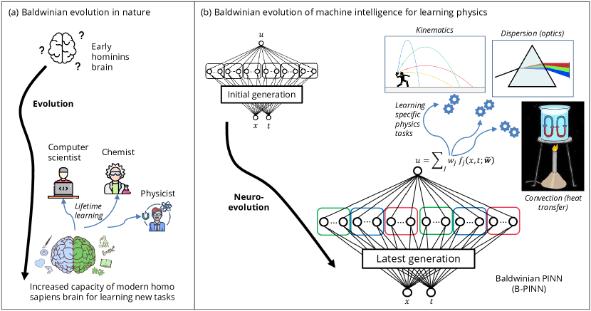
Harnessing evolutionary procedures to optimize neural networks lends much greater versatility relative to other meta-learning approaches in terms of jointly crafting network architectures, initial network connection strengths, as well as learning algorithms, all through the use of potentially non-differentiable fitness functions [20]. Such biological “neuroevolution” [21, 22] precludes the need for explicit parameterization of tasks, facilitating generalization over task distributions comprising any broad mix of ODE/PDEs, ICs, and BCs. The physics-based lifetime learning of the neural network can be accelerated by reduction to a least-squares learning problem in its output layer, making Baldwinian evolution computationally feasible. Such a least-squares formulation yields a closed-form result by means of the Moore-Penrose pseudoinverse and guarantees zero physics-informed loss given a sufficiently overparameterized network. The closed-form expression vastly reduces (or even eliminates) the need for iterative parameter updates to enable extremely fast lifetime learning of desired physics. Critically, the evolutionary search procedure is inherently highly parallelizable, thereby allowing for efficient meta-learning at scale by capitalizing on state-of-the-art advances in multi-CPU/GPU hardware infrastructure.

Neural Baldwinism thus makes it possible to achieve generalizable PINNs that are “genetically equipped” to perform well over a wide range of physics tasks. The evolved models are referred to as Baldwinian PINNs (B-PINNs), and are demonstrated in this study to be broadly applicable to the simulation of families of linear and nonlinear ODE/PDEs encompassing diverse physical phenomena such as particle kinematics, heat and mass transfer, and reaction-diffusion. These B-PINNs are capable of fast and accurate physics-aware predictions on previously unseen tasks, demonstrating up to several orders of magnitude computation speedup along with an order of magnitude improvement in prediction accuracy relative to recent meta-learned PINN results [15].

2 Results

2.1 Problem setup

We consider a physical phenomena of interest to be represented by a set of training tasks belonging to some underlying task-distribution $p(\mathbfcal{T})$, e.g., a family of PDEs spanning different PDE parameters, ICs and/or BCs. We seek to discover generalizable PINN models capable of fast, accurate, and physics-aware predictions on unseen scenarios, i.e., any new task from the distribution, $\mathcal{T}_{i}\backsim p(\mathbfcal{T})$, by learning the underlying governing physics.

For simplicity of exposition, let us consider a problem with single spatial dimension $x$, time dimension $t$, and a single variable of interest $u$. In general, PINNs can learn a mapping between the input variables $(x,t)$ and the output variable $u$ while satisfying specified governing equations representing the physical phenomenon or dynamical process of interest:

PDE: $$\mathcal{N}_{\vartheta}[u(x,t)] =h(x,t), x\in\Omega,t\in(0,T]$$ (1a)

IC: $$u(x,t=0) =u_{0}(x), x\in\Omega$$ (1b)

BC: $$\mathcal{B}[u(x,t)] =g(x,t), x\in\partial\Omega,t\in(0,T]$$ (1c)

where the general differential operator $\mathcal{N}_{\vartheta}[u(x,t)]$ contains PDE parameters $\vartheta$ and can include linear and/or nonlinear combinations of temporal and spatial derivatives, and $h(x,t)$ is an arbitrary source term in the domain $x\in\Omega,t\in(0,T]$. The IC (Eq. 1b) specifies the initial state, $u_{0}(x)$, at time $t=0$, and the BC (Eq. 1c) specifies that $\mathcal{B}[u(x,t)]$ equates to $g(x,t)$ at the domain boundary $\partial\Omega$.

PINNs can arrive at an accurate and physics-compliant prediction $u(x,t)$ for any target scenario by minimizing the discrepancy between Eq. 1 and the model’s prediction at all training samples, even in the absence of labelled data.

2.2 A two-stage stochastic programming formulation

Without loss of architectural generality, the B-PINNs are assigned the form of a multilayer perceptron (MLP) with proven representation capacity [23, 24, 25], thereby ensuring the ability to learn a diversity of tasks. Its output $u(x,t)$ can be written as:

$$u(x,t)=\sum_{j}w_{j}f_{j}(x,t;{\bf\it\tilde{w}})$$ (2)

where ${\bf\it w}=[\dots w_{j}\dots]^{T}$ are the output layer weights, and $f_{j}(x,t;{\bf\it\tilde{w}})$’s represent nonlinear projections of the input variables with the hidden layers’ weights ${\bf\it\tilde{w}}$. The connection strengths ${\bf\it\tilde{w}}$ are drawn from a probability distribution defined by a dimensionally reduced set of network hyperparameters $\theta$ (see example in Section 4.1), that are assigned at birth as per Baldwinian evolution.

The model’s reaction to a given environment—i.e., finding the best set of $w_{j}$’s such that the B-PINN’s output satisfies Eq. 1 for a specific physics task $\mathcal{T}_{i}$—can be reduced to a physics-based least-squares problem:

$$\operatorname*{arg\,min}_{{\bf\it w}}\ \mathbf{(\mathbf{A}_{{\bf\it\tilde{w}}}^{\mathcal{T}_{i}}{\bf\it w}-\mathbf{b}^{\mathcal{T}_{i}})^{T}}(\mathbf{A}_{{\bf\it\tilde{w}}}^{\mathcal{T}_{i}}{\bf\it w}-\mathbf{b}^{\mathcal{T}_{i}})+\lambda{\bf\it w}^{\mathbf{T}}{\bf\it w}$$ (3)

where $\mathbf{A}_{{\bf\it\tilde{w}}}^{\mathcal{T}_{i}}{\bf\it w}$ is obtained by substituting the model’s output into the left hand side of Eq. 1 for a given set of collocation points, and $\mathbf{b}^{\mathcal{T}_{i}}$ represents the corresponding right hand side of Eq. 1. The learning hyperparameter $\lambda\geq 0$ reduces the $L^{2}$-norm of the least-squares solution, thereby improving the solution numerically. Detailed derivations, including information on construction of matrix $\mathbf{A}_{{\bf\it\tilde{w}}}^{\mathcal{T}_{i}}$ and vector $\mathbf{b}^{\mathcal{T}_{i}}$, are provided in Section 4.2.

Eq. 3 yields a closed-form result when using the Moore-Penrose generalized inverse, permitting extremely fast learning (order of milli-seconds in our experiments) for physics-compliant prediction. Similar least-squares formulations studied in the literature have been shown to be competitive with, or faster than, widely-used numerical solvers such as the finite element method [26, 27].

Going beyond specialization to a single physics task by means of Eq. 3, we mathematically formulate the search for B-PINN models that can generalize to a whole family of PDEs as the following two-stage stochastic optimization problem [19]:

$$\min_{\theta,\lambda}\operatorname{\mathbb{E}}_{\mathcal{T}_{i}\backsim p(\mathbfcal{T})}\operatorname{\mathbb{E}}_{{\bf\it\tilde{w}}\backsim p_{\theta}(\mathbfcal{{\bf\it\tilde{w}}})}[\tau_{LSE}\ l_{LSE}({\bf\it w^{*}})+\tau_{MSE}\ l_{MSE}({\bf\it w^{*}})]\quad,\tau_{LSE}\geq 0,\tau_{MSE}\geq 0$$ (4)

where the solution ${\bf\it w^{*}}$ of the second stage problem:

$${\bf\it w^{*}}=\operatorname*{arg\,min}_{{\bf\it w}}\ \mathbf{(\mathbf{A}_{{\bf\it\tilde{w}}}^{\mathcal{T}_{i}}{\bf\it w}-\mathbf{b}^{\mathcal{T}_{i}})^{T}}(\mathbf{A}_{{\bf\it\tilde{w}}}^{\mathcal{T}_{i}}{\bf\it w}-\mathbf{b}^{\mathcal{T}_{i}})+\lambda{\bf\it w}^{\mathbf{T}}{\bf\it w}$$ (5)

provides optimal output layer weights that allow the model to specialize to any realization of task $\mathcal{T}_{i}\backsim p(\mathbfcal{T})$ for the given network’s ${\bf\it\tilde{w}}\backsim p_{\theta}(\mathbfcal{{\bf\it\tilde{w}}})$.

The first stage optimization objective is defined by the weighted sum of the physics learning proficiency, i.e., sum of squared residuals or least-squares error (LSE),

$$l_{LSE}({\bf\it w^{*}})=\mathbf{(\mathbf{A}_{{\bf\it\tilde{w}}}^{\mathcal{T}_{i}}{\bf\it w^{*}}-\mathbf{b}^{\mathcal{T}_{i}})^{T}}(\mathbf{A}_{{\bf\it\tilde{w}}}^{\mathcal{T}_{i}}{\bf\it w^{*}}-\mathbf{b}^{\mathcal{T}_{i}})$$ (6)

and the actual predictive performance, i.e., mean squared error (MSE),

$$l_{MSE}({\bf\it w^{*}})=\frac{1}{n}\sum_{s=1}^{n}\ (u_{s}^{label}-\sum_{j}w_{j}^{*}f_{j}(x_{s},t_{s};{\bf\it\tilde{w}}))^{2}$$ (7)

given labelled data $u_{s}^{label},s=1,...,n$, over the task distribution $p(\mathbfcal{T})$ and the network connections’ distribution $p_{\theta}(\mathbfcal{{\bf\it\tilde{w}}})$.

2.3 Evolving B-PINNs

We examine the efficacy of Baldwinian evolution for learning physics (Algorithm 1 and Algorithm 2 in Section 4.4) as formalized in the two-stage stochastic programming problem. As this study focuses on the paradigm of Baldwinian evolution as a pathway towards generalizable neural physics solvers, other combinations of neuroevolution or lifetime learning algorithms may be used.

In the spirit of the Baldwin effect, the learned output layer ${\bf\it w}$ is the outcome of lifetime learning and not directly inherited by the next generation of offspring [28]; only the network and learning hyperparameters $(\theta,\lambda)$ are subjected to evolutionary variation and inheritance. In this study, we employ the state-of-the-art covariance matrix adaptation evolution strategy (CMA-ES) [29] for evolving the these hyperparameters.

One key advantage of neuroevolution is that the fitness evaluations (population size $n_{pop}$ $\times$ number of random tasks $n_{task}$) required each iteration can be easily parallelized across multiple GPUs to fully harvest any hardware advantage. In particular, we utilized the JAX framework to harness previously reported performance improvements for automatic differentiation and linear algebra operations [30, 31]. The experimental study is performed on a workstation with an Intel Xeon W-2275 Processor and 2 NVIDIA GeForce RTX 3090.

Several ODE/PDE problems which are representative of real-world phenomena are used to demonstrate Baldwinian evolution for physics in the following sections. Table 1 summarizes various neuroevolution and B-PINN lifetime learning configurations and performance on their respective test tasks.

2.4 Learning to solve and generalize linear ODE/PDEs

2.4.1 Convection-diffusion

The first example is the convection-diffusion problem. The steady-state convection-diffusion equation is a ubiquitous physics model that describes the final distribution of a scalar quantity (e.g. mass, energy, or temperature) in the presence of convective transport and diffusion [32]. Solutions to this physics are key to characterizing, understanding and design of many systems, including microfluidic chip cooling in electronics [33]. The 1D equation is defined as:

$$\text{(Problem 1)}\quad\quad\alpha\frac{du}{dx}-\frac{d^{2}u}{dx^{2}}=0\quad,x\in[0,1]$$ (8)

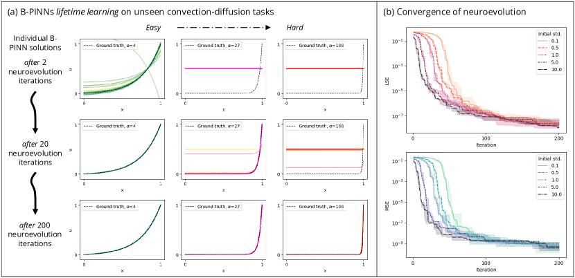
subject to BCs $u(x=0)=0$; $u(x=1)=1$. These real-world problems have characteristic physics that vary with non-dimensional constants such as the Peclet number $Pe$ (ratio of convection to diffusion) [34]. Hence, it is helpful to learn a PINN model that can return $u(x)$ for a diverse range of $\alpha$ (related to $Pe$ for this class of problems). The training tasks consist of $\alpha=\{5,10,...,100\}$, encompassing both smoother output patterns at lower $\alpha$ and very high gradient patterns at higher $\alpha$ which can be challenging both for PINNs to learn by means of stochastic gradient descent (SGD) [13, 9] and for classical numerical methods [35].

The predictive performance of the learned model is evaluated for an unseen range of test tasks, i.e., $\alpha=\{1,2,...,110\}$. The efficacy of Baldwinian evolution is demonstrated in Figure 2, with the successful evolution of B-PINNs which can learn an extremely accurate solution on new test tasks in milli-seconds. The learned solutions can achieve an average MSE of 5.8$\mathrm{e}{-9}$ $\pm$9.9$\mathrm{e}{-9}$ ($n=110$ tasks $\times$ 5 individual runs) after 200 neuroevolution iterations.

Figure 2: (a) Solution of 20 individual B-PINN models sampled from the CMA-ES search distribution (initial std. = 1), for unseen convection-diffusion tasks $\alpha=\{4,27,108\}$. The task is more challenging with increasing $\alpha$. Baldwinian evolution is effective for evolving good B-PINN models which can generalize across different difficulties. (b) Baldwinian evolution demonstrates effective LSE and MSE convergences on convection-diffusion problem, for different CMA-ES initial std. values (best std. = 1). The bold lines indicate their median convergence path from 5 individual runs, and the shaded areas indicate their interquartile ranges.

2.4.2 Family of linear PDEs (convection, diffusion, and dispersion)

Figure 3: (a) Schematic to illustrate new tasks arising from family of linear PDEs problem: S1 change to new PDE and IC profile for $t\in[0,2]$ (same time domain as train tasks), and S2 projection to longer time domain $t\in[0,4]$. (b) Solution for unseen linear PDE tasks obtained by best evolved B-PINN sampled from the center of CMA-ES search distribution after 500 iterations with initial std. = 5 (they are visually indistinguishable from the ground truth). (c) The mean MSE over $n=87$ test tasks for 2 test scenarios described in (a) are below $5\mathrm{e}{-5}$. (d) Baldwinian evolution demonstrates effective LSE and MSE convergences for different CMA-ES initial std. values, with a superior performance given by std. = 5 and 10. The bold lines indicate their median convergence path from 5 individual runs, and the shaded areas indicate their interquartile ranges.

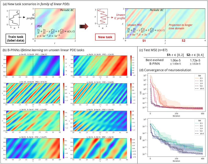
Next, we extend B-PINNs to a family of linear PDEs. This PDE family is a further generalization of the convection-diffusion equation:

$$\text{(Problem 2)}\quad\frac{du}{dt}+\alpha\frac{du}{dx}-\gamma\frac{d^{2}u}{dx^{2}}+\delta\frac{d^{3}u}{dx^{3}} =q(x,t)\quad,x\in[0,1],t\in(0,2]$$ (9a)

$$q(x,t) =\sum_{j=1}^{J}A_{j}\text{sin}(\omega_{j}t+\frac{2\pi l_{j}x}{L}+\varphi_{j})$$ (9b)

with IC $u(x,0)=q(x,0)$ and periodic BC $u(0,t)=u(1,t)$. Eq. 9 models the time evolution of a scalar quantity in the presence of physics phenomena such as convection ($\frac{du}{dx}$ component), diffusion ($\frac{d^{2}u}{dx^{2}}$ component), and dispersion ($\frac{d^{3}u}{dx^{3}}$ component), and a rich diversity of dynamical processes can be generated from different PDE and IC combinations [36, 37]. $q(x,t)$ is a source term, with the different $q(x,t=0)$ being corresponding IC profiles. We consider the following PDE scenarios: $\alpha=1$, $\gamma=\{0,5\mathrm{e}{-4},1\mathrm{e}{-3}\}$, $\delta=\{0,5\mathrm{e}{-4},1\mathrm{e}{-3}\}$. The ratio between $\alpha$, $\gamma$, and $\delta$ determine non-dimensional constants such as $Pe$, and consequently, the systems’ characteristic physics. $q(x,t)$ comprises scenarios with $J=5$, $L=6$ and coefficients sampled uniformly from $A_{j}\in[-0.8,0.8]$, $\omega_{j}\in[-2,2]$, $l_{j}\in[0,1,2,3,4]$, $\varphi_{j}\in[-\pi,\pi]$. The training set comprises 108 tasks with different PDE and IC combinations.

The effective generalization of a B-PINN to an entire PDE family with diverse output patterns is demonstrated on 2 task scenarios: S1 shows successful learning of $u(x,t)$ for $t\in[0,2]$ on unseen set of PDEs, which include changes to PDE parameters ($\gamma$ and $\delta$) and the source term / IC $q$; while S2 shows effective extrapolation of solution to a longer time domain, i.e., $t\in[0,4]$. For both scenarios, the B-PINNs learn the solution accurately in milli-seconds. The average MSE given by a successfully evolved B-PINN (sampled from the center of CMA-ES search distribution from the best run) over all test tasks ($n=87$) for S1 and S2 are 1.06$\mathrm{e}{-5}$ $\pm$1.60$\mathrm{e}{-5}$ and 1.72$\mathrm{e}{-5}$ $\pm$3.02$\mathrm{e}{-5}$, respectively. Illustrative results are in Figure 3.

Interestingly, the B-PINNs maintain good accuracy on tasks from S2, whereby the evolved B-PINN model first learns $u(x,t)$ for $t\in[0,2]$,before using the learned solution $u(x,t=2)$ as new IC for $t\in[2,4]$. This is achievable because Baldwinian evolution does not require parameterization for the tasks, and B-PINNs can generalize to new ICs, BCs, and PDE source terms despite being black-box functions. This is tricky for existing meta-PINN methods as they require interpolation across a potentially infinitely large distribution of tasks (e.g. possible BCs or ICs), in contrast to the lifetime learning encapsulated in the Baldwinian paradigm. Additional results illustrating the ability of B-PINNs to perform well despite variations in the lifetime learning task objectives (e.g., solving for different time durations) are in  B.1.1, further emphasizing the merits of Baldwinian evolution for physics.

2.5 Learning to solve and generalize nonlinear ODE/PDEs

Figure 4: (a) Solution of 20 individual B-PINN models sampled from the CMA-ES search distribution (initial std. = 0.5), for unseen kinematics tasks. (b) Solution of B-PINN model sampled from the center of CMA-ES search distribution after 100 iterations (initial std. = 1), for unseen 6D diffusion-reaction task. The solutions shown in (a) and (b) are visually indistinguishable from the ground truth. Baldwinian evolution demonstrates effective LSE and MSE convergence on both (c) kinematics and (d) 6D parametric diffusion-reaction problem, for different CMA-ES initial std. values. The bold lines indicate their median convergence path from 5 individual runs, and the shaded areas indicate their interquartile ranges.

2.5.1 Kinematics

Extending beyond linear ODE/PDEs, B-PINNs are applied to nonlinear kinematics equations. Assuming a ball is thrown at specific launch angle $a_{0}$ and initial velocity $vel_{0}$, the following 2D kinematics equations describe the ball’s motion under the influence of gravity $g$ and air resistance $R$:

$$\text{(Problem 3)}\quad\quad\frac{d^{2}x}{dt^{2}}+R\frac{dx}{dt} =0\quad\quad,t\in(0,T]$$ (10a)

$$\frac{d^{2}y}{dt^{2}}+R\frac{dy}{dt} =-g\quad\ ,t\in(0,T]$$ (10b)

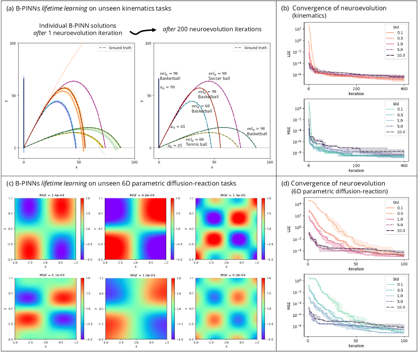
subject to ICs $x(t=0)=0,\frac{dx}{dt}(t=0)=vel_{0}\times\mathrm{cos}(\frac{a_{0}\pi}{180})$; $y(t=0)=0,\frac{dy}{dt}(t=0)=vel_{0}\times\mathrm{sin}(\frac{a_{0}\pi}{180})$. The air resistance $R=\frac{1}{2}\frac{\rho C_{d}A}{m}V$ is related to air density $\rho$, object properties (drag coefficient $C_{d}$, cross-sectional area $A$, and mass $m$), and object velocity $V=\sqrt{(dx\mathrm{/}dt)^{2}+(dy\mathrm{/}dt)^{2}}$, hence the equations are nonlinear with respect to $x$ and $y$. The 150 training tasks comprise different launch angles $a_{0}\in[15,85]$, initial velocity $vel_{0}\in[10,110]$, and object properties $C_{d}\in[0.2,0.7]$, $A\in[0.00145,0.045]$, $m\in[0.046,0.6]$ as may be representative of different projectiles (e.g., baseball, basketball). $g$ and $\rho$ are assumed to be $9.8$ and $1.3$ respectively.

The B-PINN learns the horizontal and vertical position $x(t)$ and $y(t)$ of the object via iterative least-squares computation (see Section 4.2) with a fixed number of nonlinear iterations $N=15$. 100 test tasks encompassing different $a_{0}\in[5,90]$, $vel_{0}\in[8,98]$, and $C_{d}$ are constructed to assess generalizability. Results presented in Figure 4a-b show that B-PINNs learn very accurate solutions (MSE $=$ 2.2$\mathrm{e}{-8}$ $\pm$1.3$\mathrm{e}{-7}$) in milli-seconds.

2.5.2 Set of nonlinear PDEs

The Baldwinian evolution of physics is further demonstrated on 5 nonlinear PDE problems such as the Burger’s equation [38], nonlinear Allen-Cahn equation and nonlinear reaction-diffusion equation [39], as per recent meta-learning PINN study [15] and described in Section 4.5.

A key difference between this study and meta-learning of PINNs in [15] is the availability of data for training tasks. On the test tasks, the evolved B-PINNs can achieve $\backsim 1$ order of magnitude lower relative norm error relative to [15]. Crucially, the computation time for B-PINN for new predictions is at most two seconds whereas the meta-learning approach may take more than 500 seconds (2 orders of magnitude acceleration). Complete quantitative results are summarized in Table 2. Representative B-PINN results on 6D parametric diffusion-reaction problem are presented in Figure 4c-d.

The versatility of Baldwinian evolution is also key here as we can accelerate the B-PINN’s lifetime learning by using a much coarser discretization and smaller number of nonlinear iterations during training while still learning a good solution on test tasks with finer (e.g., 16$\times$) discretization and more (e.g., 2$\times$) nonlinear iterations.

2.6 Ablation study and in-depth analysis

We further investigate the advantages of Baldwinian evolution via an ablation study using the convection-diffusion and kinematics examples.

As a baseline, we train DNN and PINN models with SGD (ADAM) based on data-driven loss and PINN (data and physics) loss respectively to make direct prediction for unseen tasks based on interpolation. For completeness, we explore different MLP architectures and configurations as per Table 3 and Section 4.7. This approach has two drawbacks: i) predictions for the new task do not incorporate the physics prior; ii) the new tasks must follow a priori determined input parameterization. For example, DNN and PINN models for convection-diffusion can be set-up with $(x,\alpha)$ as input to enable predictions for different $\alpha$s.

To address the first drawback, we incorporate physics learning—similar to B-PINN’s lifetime learning, but with SGD-learned nonlinear projections of input variables—to further optimize the output layer weights by pseudoinverse. As the pseudoinverse solution is highly dependent on the learning hyperparameter $\lambda$, we perform a grid search across $\lambda=\{1\mathrm{e}{-2},1\mathrm{e}{-4},1\mathrm{e}{-6},1\mathrm{e}{-8},1\mathrm{e}{-10},1\mathrm{e}{-12},0\}$, and present the solution associated with the lowest LSE.

The performance of DNNs and PINNs with different model configurations and prediction modes (i.e., direct DNN/PINN prediction vs. additional pseudoinverse step) across 5 runs are summarized in Table 4.

Interestingly, PINNs do not outperform DNNs for direct prediction on test tasks (e.g., MSE for convection-diffusion for different model configurations range from $1.7\mathrm{e}{-4}$ to $1.2\mathrm{e}{-2}$ for DNN, and from $1.9\mathrm{e}{-3}$ to $3.4\mathrm{e}{-1}$ for PINN), suggesting that additional physics prior during PINN training may not always benefit generalization in the absence of additional physics-aware training. However, combining PINNs with an additional pseudoinverse step can achieve better generalization performance than DNN (comparing their respective best configurations), indicating that the additional physics prior assists the SGD-trained PINNs in learning a more physics-compliant projection (${\bf\it\tilde{w}}$). This improvement is especially remarkable for nonlinear kinematics (i.e., the best MSE for DNN and PINN improves from $3.0\mathrm{e}{0}$ to $4.4\mathrm{e}{-5}$ and $1.3\mathrm{e}{0}$ to $7.9\mathrm{e}{-6}$ respectively after pseudoinverse), potentially because the training distribution is sparser relative to the larger variation in output patterns.

Figure 5: The generalization performance of the best DNN, PINN, and B-PINN models are compared, across 110 convection-diffusion and 100 kinematics test tasks. Model-1a: deep architecture with tanh activations (network weights initialized by Xavier method); Model-1b: deep architecture with sin activations (network weights initialized by He method); Model-2a: shallow architecture with tanh activations (network weights initialized by Xavier method). The bold solid and dashed lines indicate the median MSE from 5 individual runs, and the shaded areas indicate their interquartile ranges.

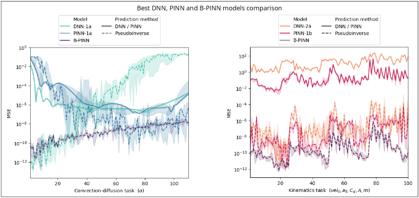
While both DNN and PINN models can learn highly accurate solutions via the pseudoinverse, this improvement is only observed in a few individual models and the SGD-learned projections are not as generalizable as the B-PINN. Prediction accuracy on individual test tasks by the best DNN, PINN, and B-PINN configurations are compared in Figure 5. While the best DNN configuration (deep architecture with tanh activations; network weights initialized by Xavier method) with pseudoinverse can be more accurate than B-PINN on convection-diffusion tasks at lower $\alpha$, solution quality deteriorates quickly at larger $\alpha$. Interestingly, PINNs with the same configuration (and pseudoinverse) show the opposite trend, highlighting the challenge of obtaining a generalizable model for entire task distributions through SGD, in contrast to Baldwinian evolution.

On average, direct prediction produces better results than pseudoinverse for convection-diffusion. For example, the MSE with and without pseudoinverse are $2.3\mathrm{e}{-4}$ and $2.8\mathrm{e}{-2}$, and $1.9\mathrm{e}{-3}$ and $7.2\mathrm{e}{-3}$ for the best-configured DNN and PINN respectively. The pseudoinverse cannot jointly minimize both PDE and IC/BC towards a sufficiently small error from SGD-learned projections, leading to a significantly worse outcome than direct prediction for some tasks. We also observe that deep architecture models generally perform better than shallow models despite the smaller number of weights in the output layer, potentially because they learn better nonlinear projections.

Critically, these results suggest that an additional step of physics-based lifetime learning (i.e. pseudoinverse) on any new task is important, and that SGD-trained models, in many instances, do not learn good projections across task distribution for the pseudoinverse, thereby negatively impacting their generalizability relative to B-PINNs. More importantly, there is no obvious way to incorporate pseudoinverse into gradient descent, making a strong case for Baldwinian evolution of physics.

3 Discussion

We study an evolutionary computation approach to tackle the meta-learning of PINNs through the lens of the Baldwin effect, such that the evolved B-PINNs can rapidly specialize as neural physics solvers to specific task from a family of governing differential equations. The method is demonstrated to be broadly applicable to the learning of different linear and nonlinear ODE/PDEs encompassing diverse physical phenomena such as reaction-diffusion, particle kinematics, and heat and mass transfer. Relative to recent meta-learned PINNs, B-PINNs can accelerate the physics-aware predictions by several orders of magnitude, while improving the prediction accuracy by up to one order. A B-PINN is thus in the image of precocial species with accelerated learning ability at birth.

The lifetime learning encapsulated in the Baldwinian paradigm does not require a priori parameterization for the task scenarios, permitting both flexible generalization to new ICs, BCs, and PDE source terms, and variations in the lifetime learning task objectives (e.g., different domain and/or sample size). This allows B-PINNs to be useful in applications when large number of evaluations with a priori unknown input conditions are sought, e.g. generative design or what-if analysis. In addition, results in Section 2.4.2 suggest that B-PINNs could be suited to the continual modelling of dynamical systems through its versatility in handling ICs and ability to rapidly model and stitch time windows together with minimal error [40, 41].

In the context of recent interest in foundation models for scientific machine learning [42], specifically through the use of neural operators or neural PDE solvers, our experiments showing accurate and fast generalization across families of linear and nonlinear ODE/PDEs suggest that Baldwinian learning can be an alternate route to such flexible and generalizable machine intelligence models. It will be interesting to test the limits to which B-PINNs can learn across broad classes of physics phenomena and/or differential operators in future work.

4 Methods

4.1 B-PINN model architecture and network connections at birth

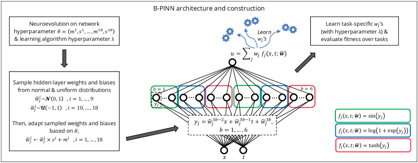
In the present study, our B-PINNs are designed to have weights and biases in the nonlinear hidden layers fixed to random values at birth—a randomized neural networks setup [43, 44]—drawn from a probability distribution defined by a dimensionally reduced set of network hyperparameters $\theta$. Both normal and uniform distributions for the weights and biases are possible for the randomized PINNs [26, 27]. Similarly, smooth nonlinear activations such as sin, softplus, and tanh are common in PINN literature, and can be advantageous for different problems. For greater generalizability, we apply both distributions for setting weights and biases and all three activations to different hidden layer blocks in the B-PINN models.

Hence, the base B-PINNs use a single hidden layer architecture which is segmented into $3\times 2=6$ unique blocks, with the weights and biases from 3 blocks sampling from normal distributions and the weights and biases from another 3 blocks sampling from uniform distributions. Each block has a fixed number of neurons ($n_{neuron}$ = 150 or 200). Assuming 2 input variables $(x,t)$, we can write the output $f_{j}$ for all the neurons $j=1,...,n_{neuron}$ in a nonlinear hidden-layer block as:

$$y_{j} =\tilde{w}_{j}^{3b-2}x+\tilde{w}_{j}^{3b-1}t+\tilde{w}_{j}^{3b}$$ (11a)

$$f_{j}(x,t;{\bf\it\tilde{w}}_{j}) =\varphi^{b}(y_{j})$$ (11b)

for each of the blocks $b=1,...,6$, where the activation $\varphi^{b}$ can be sin ($b=1,4$), softplus ($b=2,5$), or tanh ($b=3,6$). The $\tilde{w}_{j}^{i}$’s are weights and biases with their own distributional mean $m^{i}$ and spread $s^{i}$, $i=1,...,18$. Their values can be obtained by the following sampling procedure:

$$\tilde{w}_{j}^{i}\sim\mathcal{N}(0,1)\quad\text{or}\quad\tilde{w}_{j}^{i}\sim\mathcal{U}(-1,1)$$ (12a)

$$\tilde{w}_{j}^{i}\leftarrow\tilde{w}_{j}^{i}\times s^{i}+m^{i}$$ (12b)

The base B-PINN model is depicted in Figure 6. Given the B-PINNs’ configuration, a set of network hyperparameters $\theta=(m^{1},s^{1},...,m^{18},s^{18})$ control the distributional mean and spread of the weights and biases in different blocks. Together with the learning hyperparameter $\lambda$, they can significantly affect the lifetime learning performance. Since the neuroevolution only searches the distribution parameters for groups of weights instead of evolving each individual weight in the nonlinear hidden layer, the reduced dimensionality is more effectively searched by today’s evolutionary algorithms.

Figure 6: Schematic of B-PINNs architecture used in present study and procedure to obtain nonlinear hidden layers’ connections ${\bf\it\tilde{w}}$’s from the evolved network hyperparameter $\theta$ for learning task-specific outputs.

4.2 B-PINNs lifetime learning

The lifetime learning procedure of the B-PINNs occurs only in the linear output layer of the network, i.e., finding the best set of $w_{j}$’s such that the output $u(x,t)=\sum_{j}w_{j}f_{j}(x,t;{\bf\it\tilde{w}})$ satisfies the governing equations in Eq. 1 for a specific task. Given a set of collocation points $(x_{i}^{pde},t_{i}^{pde}),i=1,...,n_{pde},(x_{i}^{ic},0),i=1,...,n_{ic},(x_{i}^{bc},t_{i}^{bc}),i=1,...,n_{bc}$ sampled from the respective domain, the following system of equations can be formed:

$$\left[\begin{array}[]{ccc}\dots&\mathcal{N}_{\vartheta}[f_{j}(x_{1}^{pde},t_{1}^{pde};{\bf\it\tilde{w}})]&\dots\\ \vdots&\vdots&\vdots\\ \dots&\mathcal{N}_{\vartheta}[f_{j}(x_{n_{pde}}^{pde},t_{n_{pde}}^{pde};{\bf\it\tilde{w}})]&\dots\\ \hdashline[2pt/2pt]\dots&f_{j}(x_{1}^{ic},0;{\bf\it\tilde{w}}_{j})&\dots\\ \vdots&\vdots&\vdots\\ \dots&f_{j}(x_{n_{ic}}^{ic},0;{\bf\it\tilde{w}})&\dots\\ \hdashline[2pt/2pt]\dots&\mathcal{B}[f_{j}(x_{1}^{bc},t_{1}^{bc};{\bf\it\tilde{w}})]&\dots\\ \vdots&\vdots&\vdots\\ \dots&\mathcal{B}[f_{j}(x_{n_{bc}}^{bc},t_{n_{bc}}^{bc};{\bf\it\tilde{w}})]&\dots\\ \end{array}\right]\left[\begin{array}[]{c}\vdots\\ w_{j}\\ \vdots\\ \end{array}\right] =\left[\begin{array}[]{c}h(x_{1}^{pde},t_{1}^{pde})\\ \vdots\\ h(x_{n_{pde}}^{pde},t_{n_{pde}}^{pde})\\ \hdashline[2pt/2pt]u_{0}(x_{1}^{ic})\\ \vdots\\ u_{0}(x_{n_{ic}}^{ic})\\ \hdashline[2pt/2pt]g(x_{1}^{bc},t_{1}^{bc})\\ \vdots\\ g(x_{n_{bc}}^{bc},t_{n_{bc}}^{bc})\\ \end{array}\right]$$ (34)

$$\mathbf{A}{\bf\it w} =\mathbf{b}$$ (35)

Note that the derivatives required to construct $\mathbf{A}$ can be easily computed by automatic differentiation [45]. The best-fit solution to the above system of linear equations with unknown ${\bf\it w}=[\dots w_{j}\dots]^{T}$ can be obtained by means of the Moore-Penrose pseudoinverse:

$${\bf\it w} =(\lambda I+\mathbf{A}^{T}\mathbf{A})^{-1}\mathbf{A}\mathbf{b} ,\text{if the system of equations in Eq. \ref{eq:leastsquares} is over-determined}$$ (36a)

$${\bf\it w} =\mathbf{A}^{T}(\lambda I+\mathbf{A}\mathbf{A}^{T})^{-1}\mathbf{b} ,\text{if the system of equations in Eq. \ref{eq:leastsquares} is under-determined}$$ (36b)

where the learning hyperparameter $\lambda\geq 0$ reduces the $L^{2}$-norm of the least-squares solution, thereby improving the solution numerically. Such a least-squares formulation yields a closed-form result in a single computation step for any linear PDE (i.e., the governing equations in Eq. 1 are all linear with respect to $u$) which encapsulates a wide class of problems in the natural world.

For nonlinear PDEs, iterative methods can be used for arriving at optimized $w_{j}$’s in B-PINNs. In this work, we use a lagging of coefficient approach which is common in numerical methods [46]. Briefly, we approximately linearize the nonlinear term(s) in Eq. 1 by substituting the output $u(x,t)=\sum_{j}w_{j}f_{j}(x,t;{\bf\it\tilde{w}})$ obtained from previous step, and iteratively solve Eq. 36 to update $w_{j}$’s for a fixed number of steps, $N$, or until a convergence criterion is reached.

Hence, the B-PINN lifetime learning is broadly applicable to both linear and nonlinear PDEs, with the psuedoinverse formulation permitting extremely fast computation for physics-compliant prediction. In addition, there is no requirement on prior labelled data for any new task as the learning can be entirely physics-based (as per conventional PINNs).

4.3 Lagging of coefficient method for nonlinear PDEs

The nonlinear equation $(\frac{d^{2}u}{dx^{2}}+\frac{d^{2}u}{dy^{2}})+u(1-u^{2})=f$ is used to demonstrate the lagging of coefficient method for computing the $w_{j}$’s in B-PINN.

We approximately linearize the nonlinear term $u(1-u^{2})$ as $u(1-\check{u}^{2})$ with $\check{u}=0$ being the initial guess solution at first iteration. The $(i\text{-th PDE sample},j\text{-th neuron})$ entry of the least squares matrix $\mathbf{A}$ in Eq. 35 now becomes:

$$\mathcal{N}_{\theta}[f_{j}(x_{i}^{pde},y_{i}^{pde};{\bf\it\tilde{w}}_{j})]=\frac{d^{2}f_{j}(x_{i}^{pde},y_{i}^{pde};{\bf\it\tilde{w}}_{j})}{dx^{2}}+\frac{d^{2}f_{j}(x_{i}^{pde},y_{i}^{pde};{\bf\it\tilde{w}}_{j})}{dy^{2}}+f_{j}(x_{i}^{pde},y_{i}^{pde};{\bf\it\tilde{w}}_{j})(1-\check{u}^{2})$$ (37)

Hence, the pseudoinverse solution ${\bf\it w}$ can be obtained from the linearized version of the equation. The solution obtained from past iteration is used to compute $\check{u}(x,y)=\sum_{j}w_{j}f_{j}(x,y;{\bf\it\tilde{w}}_{j})$ for the next iteration, until the solution ${\bf\it w}$ becomes stable or upon reaching a pre-determined number of iterations, $N$.

4.4 Baldwinian evolution algorithm and hyperparameters

Algorithm 1 Baldwinian evolution of B-PINNs

1:$p(\mathbfcal{T})$: distribution over physics tasks

2:$\mathbfcal{P}$: initial population-representation of individuals (i.e., network architecture and learning algorithm hyperparameters in B-PINN models)

3:$\mathbfcal{S}$: procedure to obtain a batch of individuals given a population-representation

4:$\mathbfcal{U}$: procedure to update a population-representation given a batch of fitness-scored individuals

5:$\mathbfcal{F}$: procedure to return fitness based on lifetime learning performance of individual given a set of tasks

6:while not done do

7:     Sample batch of individuals from population $(\theta^{g},\lambda^{g})\backsim\mathbfcal{S}(\mathbfcal{P}),g=1,...,n_{pop}$

8:     Sample batch of tasks $\mathcal{T}_{i}\backsim p(\mathbfcal{T}),i=1,...,n_{task}$

9:     for all $(\theta^{g},\lambda^{g})$ do

10:         $f^{g}=\mathbfcal{F}(\theta^{g},\lambda^{g},\{\mathcal{T}_{i},i=1,...,n_{task}\})$

11:     end for

12:     Update population based on fitness of individuals:

     $\mathbfcal{P}\leftarrow\mathbfcal{U}(\mathbfcal{P},\{(\theta^{g},\lambda^{g},f^{g}),g=1,....,n_{pop}\})$

13:end while

Algorithm 2 B-PINN lifetime learning and fitness calculation $\mathbfcal{F}$

INPUT: network architecture and learning algorithm hyperparameters $(\theta,\lambda)$, list of tasks $\mathcal{T}_{i},i=1,...,n_{task}$

OUTPUT: fitness $f$

1:$\mathbfcal{G}$: procedure to sample weights and biases in nonlinear hidden-layer(s)

2:$\mathbfcal{C}$: procedure to construct least squares problem on a set of collocation points based on underlying physics (PDEs, BCs, ICs) of the task

3:$N$: number of iterations to take during per-task “lifetime learning”: $1$ for linear PDEs, $>1$ for nonlinear PDEs

4:Sample hidden layers’ weights and biases ${\bf\it\tilde{w}}=\mathbfcal{G}(\theta)$

5:for all $\mathcal{T}_{i}$ do

6:     ${\bf\it w}=[\dots w_{j}\dots]^{T}=\mathbf{0}$ $\triangleright$ initial solution for nonlinear PDEs

7:     for $k=1,...,N$ do

8:         Construct least squares matrix and vector $(\mathbf{A},\mathbf{b})=\mathbfcal{C}(\mathcal{T}_{i},{\bf\it\tilde{w}},{\bf\it w})$

9:         Compute least-squares solution via pseudoinverse:

         ${\bf\it w}=(\lambda I+\mathbf{A}^{T}\mathbf{A})^{-1}\mathbf{A}\mathbf{b}$ , if $\mathbf{A}$ has more rows than columns

         ${\bf\it w}=\mathbf{A}^{T}(\lambda I+\mathbf{A}\mathbf{A}^{T})^{-1}\mathbf{b}$ , if $\mathbf{A}$ has more columns than rows

10:     end for

11:     ${\bf\it w}^{\mathcal{T}_{i}}\leftarrow{\bf\it w}$, $\mathbf{A}^{\mathcal{T}_{i}}\leftarrow\mathbf{A}$, $\mathbf{b}^{\mathcal{T}_{i}}\leftarrow\mathbf{b}$

12:end for

13:Compute least-squares error: $l_{LSE}=\sum_{\mathcal{T}_{i}}\mathbf{(\mathbf{A}^{\mathcal{T}_{i}}{\bf\it w}^{\mathcal{T}_{i}}-\mathbf{b}^{\mathcal{T}_{i}})^{T}}(\mathbf{A}^{\mathcal{T}_{i}}{\bf\it w}^{\mathcal{T}_{i}}-\mathbf{b}^{\mathcal{T}_{i}})$

14:Compute mean squared error: $l_{MSE}=\sum_{\mathcal{T}_{i}}\frac{1}{n}\sum_{s}^{n}(u_{s}^{label}-\sum_{j}w_{j}^{\mathcal{T}_{i}}f_{j}(x_{s},t_{s};{\bf\it\tilde{w}}_{j}))^{2}$ over the labelled data $u_{s}^{label},s=1,...,n$

15:Compute overall fitness: $f=-(\tau_{LSE}\ l_{LSE}+\tau_{MSE}\ l_{MSE})$

Algorithm 1 and Algorithm 2 describe a Baldwinian evolution procedure to solve the two-stage stochastic programming problem defined in Section 2.2. Recall a B-PINN individual can be represented by $(\theta,\lambda)$, i.e., network architecture and learning algorithm hyperparameters, during neuroevolution.

The Baldwinian evolution procedure described in Algorithm 1 is generic for neuroevolution methods, such as CMA-ES. As an instantiation of information-geometric optimization algorithms [47], CMA-ES represents the population of $(\theta,\lambda)$ in $\mathbfcal{P}$ using a multivariate normal search distribution, initialized with zeros mean and standard deviation (std.) as tuning hyperparameter. $\mathbfcal{S}$ becomes a random sampling procedure with population size or the number of individuals $n_{pop}$ to be sampled from the search distribution as hyperparameter, and $\mathbfcal{U}$ is the CMA-ES update-step [29] which iteratively adapts its search distribution based on the rank-based fitness landscape until the convergence criteria, e.g., a pre-determined number of iterations or fitness value (trade-off between computation resource and convergence) is met.

The network weights and biases can take any value from $(-\infty$, $\infty)$, hence there is no restriction to the continuous search space of $\theta=(m^{1},s^{1},...)$ representing their distributional means and spreads. The learning hyperparameter $\lambda\geq 0$ can be evolved in continuous search space and its absolute value is then used for computing the least-squares solution. In our implementation with CMA-ES, $(\theta,\lambda)$ share a same initial standard deviation, and we scale the learning hyperparameter by a factor, i.e., $\lambda\leftarrow 1\mathrm{e}{-4}\times\text{abs}(\lambda)$ during B-PINN lifetime learning to improve the convergence.

Our preliminary experiments show that the performance of Baldwinian evolution is robust across a range of CMA-ES hyperparameters such as population size and initial standard deviation (std.) of search distribution, and the number of tasks sampled for fitness evaluation per iteration. Hence, a robust setting that shows good convergence in fitness across different types of problems is chosen based on initial experiments.

In Algorithm 2, a fixed set of collocation points are used for the construction of least squares matrix and vector $(\mathbf{A},\mathbf{b})$ across the training tasks for ease of implementation. These collocation points also coincide with the location of labelled data for $l_{MSE}$ computation, although this is not a prerequisite. Similarly, the same number of nonlinear iterations $N$ is used across nonlinear training tasks sampled from the task distribution.

We found, in our preliminary experiments, that it is critical to have the $l_{MSE}$ component in the optimization objective even though the learning of future test tasks remains solely physics-based. We set $\tau_{LSE}=\tau_{MSE}=1$ as default for the computation of overall fitness, unless there is a huge difference in magnitude between $l_{LSE}$ and $l_{MSE}$ during the Baldwinian evolution of physics. In addition, we can multiply the BC/IC rows in both $\mathbf{A}$ and $\mathbf{b}$ to re-balance the importance between PDE and BC/IC errors in the least-squares solution.

4.5 Nonlinear PDE problems description

The nonlinear PDE problems (Problem 4-8) used for demonstrating the Baldwinian evolution of physics are described below. As per [15], the spatio-temporal domain in Problem 4-5 is uniformly discretized into 256$\times$100, and the 2D spatial domain in Problem 6-8 is uniformly discretized into 128$\times$128, for the test tasks. The comparison between B-PINNs and the meta-learned PINN results reported in [15] are summarized in Table 2.

4.5.1 Burgers’ equation

The Burgers’ equation consists of 16 randomly sampled train tasks and 32 uniformly sampled test tasks from the PDE parameter $\gamma\in[5\mathrm{e}{-3},5\mathrm{e}{-2}]$:

$$\text{(Problem 4)}\quad\quad\quad\quad\ \ \frac{du}{dt}+u\frac{du}{dx}-\gamma\frac{d^{2}u}{dx^{2}}=0\quad,x\in[-1,1],t\in(0,1]$$ (38)

subject to IC $u(x,t=0)=-\mathrm{sin}(\pi x)$.

4.5.2 Nonlinear heat equation

The nonlinear heat equation consists of 13 randomly sampled train tasks and 64 uniformly sampled test tasks from the PDE parameters $\gamma\in[1,\pi],k\in[1,\pi]$:

$$\text{(Problem 5)}\quad\quad\frac{du}{dt}-\gamma\frac{d^{2}u}{dx^{2}}+k\ \mathrm{tanh}(u)=f\quad,x\in[-1,1],t\in(0,1]$$ (39)

where the exact solution $u(x,t;\gamma,k)=k\mathrm{sin}(\pi x)\mathrm{exp}(-\pi kx^{2})\mathrm{exp}(-\pi t^{2})$ is used to derive the corresponding IC, BCs and source term $f$.

4.5.3 Nonlinear Allen-Cahn equation

The nonlinear Allen-Cahn equation consists of 16 randomly sampled train tasks and 32 uniformly sampled test tasks from the PDE parameter $\gamma\in(0,\pi]$:

$$\text{(Problem 6)}\quad\quad\gamma(\frac{d^{2}u}{dx^{2}}+\frac{d^{2}u}{dy^{2}})+u(u^{2}-1)=f\quad,x\in[-1,1],y\in[-1,1]$$ (40)

where the exact solution $u(x,y;\gamma)=\mathrm{exp}(-\gamma(x+0.7))\mathrm{sin}(\pi x)\mathrm{sin}(\pi y)$ is used to derive the corresponding BCs and source term $f$..

4.5.4 Nonlinear diffusion-reaction equation

The nonlinear diffusion-reaction equation consists of 22 randomly sampled train tasks and 64 uniformly sampled test tasks from the PDE parameter $\gamma\in[1,\pi],k\in[1,\pi]$:

$$\text{(Problem 7)}\quad\quad\quad\quad\ \gamma(\frac{d^{2}u}{dx^{2}}+\frac{d^{2}u}{dy^{2}})+ku^{2}=f\quad,x\in[-1,1],y\in[-1,1]$$ (41)

where the exact solution $u(x,y;\gamma,k)=k\mathrm{sin}(\pi x)\mathrm{sin}(\pi y)\mathrm{exp}(-\gamma\sqrt{kx^{2}+y^{2}})$ is used to derive the corresponding BCs and source term $f$.

4.5.5 6D parametric diffusion-reaction

The 6D parametric diffusion-reaction problem consists of 17 randomly sampled train tasks and 100 randomly sampled test tasks from the PDE/BC parameters $(\alpha_{1},\alpha_{2},\omega_{1},\omega_{2},\omega_{3},\omega_{4})$, $\alpha$’s$\in[0.1,1]$, $\omega$’s$\in[1,5]$:

$$\text{(Problem 8)}\quad\quad\ (\frac{d^{2}u}{dx^{2}}+\frac{d^{2}u}{dy^{2}})+u(1-u^{2})=f\quad,x\in[-1,1],y\in[-1,1]$$ (42)

where the exact solution $u(x,y;\alpha_{1},\alpha_{2},\omega_{1},\omega_{2},\omega_{3},\omega_{4})=\alpha_{1}\mathrm{tanh}(\omega_{1}x)\mathrm{tanh}(\omega_{2}y)+\alpha_{2}\mathrm{sin}(\omega_{3}x)\mathrm{sin}(\omega_{4}y)$ is used to derive the corresponding BCs and source term $f$.

4.6 Data generation

In this study, the ground truth is obtained by high resolution finite volume scheme for the PDE family (Eq. 9) and Burgers’ equation (Eq. 38). To alleviate convection instability, the dispersion-relation-preserving (DRP) finite volume scheme with universal limiter has been utilized [48, 49]. Other spatial derivative terms are discretized by central difference. For the temporal term, the second order TVD Runge Kutta scheme [50] is employed. For the PDE family equation, the spatial resolution, $\Delta x$, is 1/400, while temporal resolution, $\Delta t$, is 5E-5$\Delta x$; For the Burgers’ equation, the spatial resolution, $\Delta x$, is 1/512, while temporal resolution $\Delta t$, is 1E-2$\Delta x$.

4.7 Baseline SGD-trained DNN and PINN models used in ablation study

Consider the general inputs $(x,t,\vartheta)$ for the spatial-temporal domain and task parameter $\vartheta$. The data-driven loss function of a SGD-trained DNN model computes the MSE between the DNN output $u_{\text{DNN}}(x_{i},t_{i},\vartheta_{i})$ against the target $u_{i}^{label}$ over $i=1,...,n$ labelled data pooled from a batch of training tasks:

$$l_{\text{DNN}}=l_{data}=\frac{1}{n}\sum_{i=1}(u_{i}^{label}-u_{\text{DNN}}(x_{i},t_{i},\vartheta_{i}))^{2}$$ (43)

The loss function of a SGD-trained PINN model is defined as:

$$l_{\text{PINN}} =\lambda_{data}\ l_{data}+\lambda_{pde}\ l_{pde}+\lambda_{ic}\ l_{ic}+\lambda_{bc}\ l_{bc}$$ (44a)

$$l_{pde} =\frac{1}{n_{pde}}\sum_{i=1}(\mathcal{N}_{\vartheta}[u_{\text{PINN}}(x_{i}^{pde},t_{i}^{pde},\vartheta_{i})]-h(x_{i}^{pde},t_{i}^{pde}))^{2}$$ (44b)

$$l_{ic} =\frac{1}{n_{ic}}\sum_{i=1}(u_{\text{PINN}}(x_{i}^{ic},0,\theta_{i})-u_{0}(x_{i}^{ic}))^{2}$$ (44c)

$$l_{bc} =\frac{1}{n_{bc}}\sum_{i=1}(\mathcal{B}[u_{\text{PINN}}(x_{i}^{bc},t_{i}^{bc},\theta_{i})]-g(x_{i}^{bc},t_{i}^{bc}))^{2}$$ (44d)

such that the PINN output $u_{\text{PINN}}(x_{i},t_{i},\vartheta_{i})$ satisfies the Eq. 1 (i.e., PDE, IC and BC) for a set of training samples $(x_{i}^{pde},t_{i}^{pde},\vartheta_{i}),i=1,...,n_{pde},(x_{i}^{ic},0,\vartheta_{i}),i=1,...,n_{ic},(x_{i}^{bc},t_{i}^{bc},\vartheta_{i}),i=1,...,n_{bc}$ from the respective domain and task, in addition to minimizing the MSE from the labelled data. SGD-trained PINNs typically converge much slower than DNN because of the additional loss terms. We perform a coarse search for the loss balancing parameters $(\lambda_{data},\lambda_{pde},\lambda_{ic},\lambda_{bc})$ to improve the convergence of the PINN loss.

We explore deep and shallow MLP architectures for the baseline SGD-trained DNN and PINN models: 1. the deep architecture consists of similar total number of network weights as the prior B-PINN models but distributed across multiple nonlinear hidden layers with smaller number of nodes; 2. the shallow architecture has single nonlinear hidden layer and same number of nodes as B-PINN model but this necessitates more total network weights because of the additional input variables.

Each architecture further consists of 2 variants: a. tanh activation for the nonlinear hidden layers whereby the network weights are initialized by Xavier method; b. sin activation for the nonlinear hidden layers whereby the network weights are initialized by He method.

We test a range of learning rate schedules, e.g., an initial learning rate $=\{5\mathrm{e}{-4},1\mathrm{e}{-3},1\mathrm{e}{-2}\}$ for the first 40% of training iterations followed by cosine decay towards $1\mathrm{e}{-6}$. The model configurations are summarized in Table 3.

Acknowledgments

This research is supported by A*STAR under the AME Programmatic project: Explainable Physics-based AI for Engineering Modelling & Design (ePAI) [Award No. A20H5b0142].

Code availability

The example codes with detailed instructions are available at https://github.com/chiuph/Baldwinian-PINN.

Appendix A Extended Data

Table 1: Summary of neuroevolution and B-PINN’s lifetime learning configurations, and generalization performance on PINN problems in experimental study

	Task distribution		Neuroevolution / CMA-ES					B-PINN lifetime learning			Predictive performance
	Problem	No. train tasks	Batch size for task, $n_{task}$	Population size, $n_{pop}$	Max. iteration	Initial std.	Search dimension for $(\theta,\lambda)$	dim(${\bf\it w}$)	Sample size $(n_{pde},n_{ic},n_{bc})$	nonlinear iterations, $N$	No. test tasks	MSE	Time (s)
1	Convection-diffusion $x\rightarrow u$	20	10	20	200	1	25	900	1001, -, 2	-	110	5.8e-9 $\pm$ 9.9e-9	0.005 $\pm$ 0.001
2	Family of linear PDEs $(x,t)\rightarrow u$	108	15	20	500	5	37	1200	5151, 101, 50 (10201, 101, 100)	-	87	7.1e-4 $\pm$ 3.1e-3	0.122 $\pm$ 0.002
3	Kinematics $t\rightarrow(x,y)\quad\quad$	150	30	20	400	0.5	25	1800	101, 1, -	15	100	2.2e-8 $\pm$ 1.3e-7	0.039 $\pm$ 0.001
4	Burgers’ equation $(x,t)\rightarrow u$	16	5	20	200	1	37	900	13107, 257, 100 (25957, 257, 200)	5 (10)	32	2.3e-7 $\pm$ 9.6e-7	1.96 $\pm$ 0.01
5	nonlinear heat $(x,t)\rightarrow u$	13	5	20	100	5	37	900	1600, 64, 50 (25600, 256, 200)	5	64	1.3e-7 $\pm$ 4.1e-7	0.87 $\pm$ 0.02
6	Allen-Cahn equation $(x,y)\rightarrow u$	16	8	20	100	0.5	37	900	1024, -, 128 (16384, - ,512)	5 (10)	32	2.0e-7 $\pm$ 6.1e-7	1.19 $\pm$ 0.01
7	Diffusion-reaction $(x,y)\rightarrow u$	22	10	20	100	1	37	900	1024, -, 128 (16384, - ,512)	5	64	1.2e-8 $\pm$ 8.1e-8	0.58 $\pm$ 0.02
8	6D diffusion-reaction $(x,y)\rightarrow u$	17	8	20	100	1	37	900	1024, -, 128 (16384, - ,512)	5	100	1.6e-8 $\pm$ 2.5e-8	0.60 $\pm$ 0.03

Table 2: Comparison with baseline meta-learning PINN models on nonlinear benchmark problems

Problem

Method / Model

(no. test task)

Random

MAML

Center

Multitask

LMC

RBF (multiquadric)

Polynomial

B-PINN

Error

Time

Error

Time

Error

Time

Error

Time

Error

Time

Error

Time

Error

Time

Error

Time

4

Burgers’ equation $(n=32)$

1.2e-3 $\pm$1.8e-3

105 $\pm$29

1.7e-3 $\pm$3.2e-3

125 $\pm$38

9e-4 $\pm$5e-4

56 $\pm$48

7e-4 $\pm$2e-4

24 $\pm$21

8e-4 $\pm$4e-4

40 $\pm$27

8e-4 $\pm$4e-4

7 $\pm$8

7e-4 $\pm$3e-4

7 $\pm$16

3.8e-4 $\pm$6.9e-4

1.96 $\pm$0.01

5

nonlinear heat $(n=64)$

5.2e-3 $\pm$3.9e-3

156 $\pm$42

4.5e-3 $\pm$3.1e-3

188 $\pm$43

4.5e-3 $\pm$2.4e-3

96 $\pm$41

4.8e-3 $\pm$3.6e-3

49 $\pm$30

4.9e-3 $\pm$3.3e-3

59 $\pm$28

4.4e-3 $\pm$2.2e-3

35 $\pm$30

4.6e-3 $\pm$3.2e-3

38 $\pm$30

6.0e-4 $\pm$7.6e-4

0.87 $\pm$0.02

6

Allen-Cahn equation $(n=32)$

1.5e-2 $\pm$1.2e-2

496 $\pm$161

-

-

1.2e-2 $\pm$4.6e-3

201 $\pm$83

1.2e-2 $\pm$4.7e-3

120 $\pm$44

1.1e-2 $\pm$4.0e-3

120 $\pm$21

1.2e-2 $\pm$5.3e-3

68 $\pm$46

1.2e-2 $\pm$4.2e-3

44 $\pm$19

9.5e-4 $\pm$1.5e-3

1.19 $\pm$0.01

7

Diffusion-reaction $(n=64)$

1.1e-2 $\pm$6.2e-3

1073 $\pm$206

-

-

9.5e-3 $\pm$5.9e-3

426 $\pm$159

9.0e-3 $\pm$5.4e-3

243 $\pm$93

9.1e-3 $\pm$5.8e-3

302 $\pm$127

8.1e-3 $\pm$4.6e-3

280 $\pm$161

8.5e-3 $\pm$5.1e-3

249 $\pm$129

1.3e-4 $\pm$2.0e-4

0.58 $\pm$0.02

8

6D diffusion-reaction $(n=100)$

2.2e-3 $\pm$1.3e-3

612 $\pm$255

-

-

1.8e-3 $\pm$1.7e-3

494 $\pm$222

1.7e-3 $\pm$1.9e-3

431 $\pm$200

1.5e-3 $\pm$1.8e-3

428 $\pm$201

1.7e-3 $\pm$2.0e-3

375 $\pm$168

1.8e-3 $\pm$2.0e-3

496 $\pm$213

1.9e-4 $\pm$1.5e-4

0.60 $\pm$0.03

Table 3: DNN / PINN model and training configurations used in ablation study

	Problem	Model	Architecture	Activation	Initialization	No. weights	Training / ADAM optimizer
						(output layer)	Batch size for task	Max. iteration	Learning rate
1	Convection-diffusion $(x,\alpha)\rightarrow u$	1a	Deep	tanh	Xavier	2750 (50)	10	50,000	5e-4 / 5e-3 / 5e-2
		1b	Deep	sin	He	2750 (50)	10	50,000	5e-4 / 5e-3 / 5e-2
		2a	Shallow	tanh	Xavier	3600 (900)	10	50,000	5e-4 / 5e-3 / 5e-2
		2b	Shallow	sin	He	3600 (900)	10	50,000	5e-4 / 5e-3 / 5e-2
3	Kinematics $(t,vel_{0},a_{0},C_{d},A,m)\rightarrow(x,y)$	1a	Deep	tanh	Xavier	3930 (60)	30	150,000	5e-4 / 5e-3 / 5e-2
		1b	Deep	sin	He	3930 (60)	30	150,000	5e-4 / 5e-3 / 5e-2
		2a	Shallow	tanh	Xavier	6300 (1800)	30	150,000	5e-4 / 5e-3 / 5e-2
		2b	Shallow	sin	He	6300 (1800)	30	150,000	5e-4 / 5e-3 / 5e-2

Table 4: Generalization performance of DNN / PINN models in ablation study

Problem

Model

DNN

PINN

(no. test task)

Lr

5e-4

5e-3

5e-2

5e-4

5e-3

5e-2

Mode

DNN

Pseudo-inverse

DNN

Pseudo-inverse

DNN

Pseudo-inverse

PINN

Pseudo-inverse

PINN

Pseudo-inverse

PINN

Pseudo-inverse

1

Convection-diffusion $(n=110)$

1a

3.5e-4 $\pm$ 2.2e-3

1.5e-1 $\pm$ 1.1e-1

2.3e-4 $\pm$1.8e-3

3.8e-2 $\pm$7.6e-2

1.2e-2 $\pm$2.6e-2

2.3e-1 $\pm$2.8e-2

4.6e-3 $\pm$2.0e-2

1.4e-2 $\pm$4.3e-2

1.9e-3 $\pm$1.1e-2

7.2e-3 $\pm$2.5e-2

2.2e-1 $\pm$5.6e-2

2.3e-1 $\pm$2.8e-2

1b

6.9e-4 $\pm$2.2e-3

1.8e-1 $\pm$1.0e-1

1.7e-4 $\pm$1.0e-3

1.3e-1 $\pm$1.2e-1

1.9e-3 $\pm$7.4e-3

2.2e-2 $\pm$3.6e-2

1.3e-1 $\pm$9.3e-2

1.6e-1 $\pm$1.1e-1

2.1e-2 $\pm$3.5e-2

1.1e-1 $\pm$1.1e-1

3.4e-1 $\pm$3.7e-1

1.9e-1 $\pm$9.6e-2

2a

7.1e-3 $\pm$6.8e-3

2.3e-1 $\pm$4.7e-2

4.5e-3 $\pm$1.3e-2

2.2e-1 $\pm$5.3e-2

2.3e-3 $\pm$4.0e-3

2.1e-1 $\pm$7.2e-2

2.2e-1 $\pm$4.5e-2

2.3e-1 $\pm$4.9e-2

1.9e-1 $\pm$7.0e-2

2.2e-1 $\pm$5.6e-2

2.0e-1 $\pm$6.5e-2

2.1e-1 $\pm$7.8e-2

2b

6.0e-3 $\pm$7.1e-3

2.2e-1 $\pm$5.7e-2

3.8e-3 $\pm$5.0e-3

2.2e-1 $\pm$6.1e-2

2.5e-3 $\pm$5.2e-3

2.1e-1 $\pm$7.7e-2

2.2e-1 $\pm$5.1e-2

2.2e-1 $\pm$5.8e-2

2.2e-1 $\pm$5.2e-2

2.2e-1 $\pm$5.9e-2

2.1e-1 $\pm$5.8e-2

2.2e-1 $\pm$6.1e-2

3

Kinematics $(n=100)$

1a

8.5e+0 $\pm$2.8e+1

2.9e-2 $\pm$4.2e-1

3.7e+1 $\pm$8.8e+1

9.4e+2 $\pm$3.5e+3

2.0e+2 $\pm$6.2e+2

2.6e+3 $\pm$4.6e+3

1.1e+1 $\pm$3.7e+1

2.5e+2 $\pm$3.3e+3

1.9e+1 $\pm$6.0e+1

4.8e+1 $\pm$6.3e+2

2.5e+3 $\pm$4.5e+3

2.6e+3 $\pm$4.6e+3

1b

3.5e+0 $\pm$1.4e+1

3.0e-3 $\pm$4.5e-2

1.9e+1 $\pm$6.7e+1

3.2e-4 $\pm$2.9e-3

5.2e+0 $\pm$9.1e+0

2.6e+3 $\pm$4.6e+3

1.3e+0 $\pm$5.7e+0

7.9e-6 $\pm$1.1e-4

3.5e+0 $\pm$1.4e+1

1.6e-5 $\pm$1.1e-4

3.0e+3 $\pm$3.5e+3

8.1e-2 $\pm$1.6e+0

2a

3.0e+0 $\pm$4.3e+1

4.4e-5 $\pm$2.5e-4

7.9e+0 $\pm$1.6e+1

2.4e+1 $\pm$3.8e+2

1.8e+1 $\pm$2.7e+1

2.3e+2 $\pm$1.6e+3

2.8e+1 $\pm$5.5e+1

9.4e-3 $\pm$1.7e-1

3.3e+0 $\pm$6.5e+0

3.1e-4 $\pm$2.8e-3

1.5e+1 $\pm$2.9e+1

1.2e-2 $\pm$2.7e-1

2b

1.5e+1 $\pm$2.7e+1

5.2e-2 $\pm$5.4e-1

2.1e+0 $\pm$3.5e+0

2.0e-1 $\pm$2.1e+0

5.0e+2 $\pm$7.7e+2

1.4e-3 $\pm$7.9e-3

2.2e+1 $\pm$4.4e+1

4.7e-2 $\pm$3.1e-1

4.0e+0 $\pm$8.7e+0

5.2e-3 $\pm$3.5e-2

7.8e+1 $\pm$1.1e+2

5.9e-3 $\pm$3.9e-2

A.1 Tables

Four tables are included to provide a more comprehensive description of the various experimental studies and model performance.

Table 1 summarizes the Baldwinian evolution and B-PINN lifetime learning configurations for 8 ODE and PDE problems, and their subsequent performance on test tasks.

Table 2 compares the generalization performance and the compute cost between B-PINNs and several meta-learning PINN models as per [15].

Table 3 and Table 4 give the DNN / PINN model and training configurations and their subsequent performance on test tasks for the ablation study.

Appendix B Additional visualization results

B.1 Family of linear PDEs problem

B.1.1 Prediction on new time interval

The experimental results in Section 2.4.2 show that B-PINNs trained on a set of linear PDE tasks for $t\in[0,2]$, are capable of learning time-dependent solution $u(x,t)$ on a set of test tasks for unseen PDEs and ICs, as well as for a longer (2 $\times$) time domain by performing the learning twice, i.e., for $t\in[0,2]$ and then using the learned solution $u(x,t=2)$ as new IC for $t\in[2,4]$. Recall that the average MSE given by the best evolved B-PINN model (sampled from the center of CMA-ES search distribution from the best run) over all test tasks for $t\in[0,2]$ and $t\in[0,4]$ are 1.06$\mathrm{e}{-5}$ $\pm$1.60$\mathrm{e}{-5}$ and 1.72$\mathrm{e}{-5}$ $\pm$3.02$\mathrm{e}{-5}$, respectively.

We further demonstrate the versatility of B-PINNs by changing the time domain of interest in the test tasks to $t\in[0,3]$. From the best evolved B-PINN model, we can obtain the prediction on new tasks in the following ways: P0 the solution for the original time domain $t\in[0,2]$ via physics-based lifetime learning, and the extended time $t\in[2,3]$ based on neural network interpolation; P1 the solution for original and extended time domain $t\in[0,3]$ altogether via physics-based lifetime learning; P2 physics learning the solution for the first 2s time $t\in[0,2]$, before using the learned solution $u(x,t=2)$ as new IC for next 2s time $t\in[2,4]$; P3 physics learning the solution for the first 2s time $t\in[0,2]$, before using the learned solution $u(x,t=2)$ as new IC for next time domain $t\in[2,3]$.

Figure 7: Solution for unseen linear PDE tasks on $t\in[0,3]$ obtained by best evolved B-PINN (sampled from the center of CMA-ES search distribution after 500 iterations with initial std. = 5) using different ways P0-P3.

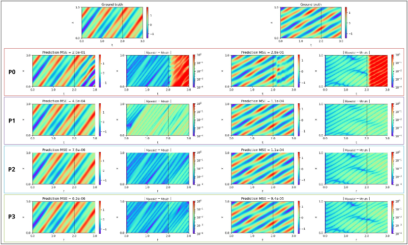
Figure 7 shows the B-PINN’s solution obtained using different ways P0-P3 on selected test tasks. Their MSE results over all test tasks for $t\in[0,3]$ are 5.35$\mathrm{e}{-2}$ $\pm$6.08$\mathrm{e}{-2}$ (P0), 4.24$\mathrm{e}{-5}$ $\pm$1.04$\mathrm{e}{-5}$ (P1), 1.47$\mathrm{e}{-5}$ $\pm$2.32$\mathrm{e}{-5}$ (P2), and 1.43$\mathrm{e}{-5}$ $\pm$2.22$\mathrm{e}{-5}$ (P3), respectively. The performance of P0 is significantly worse than P1-P4, as expected, because of the physics-agnostic extrapolation. The B-PINNs can versatily learn the solutions on extended time domain in a single pseudoinverse solve (P1), although the most accurate solutions are given by P2 and P3.

Figure 8: B-PINN’s solution (run no. 2) vs. ground truth on 5 selected tasks, and the position of their accuracy along the MSE spectrum (pooled from $n=87$ test tasks $\times$ 5 individual runs with initial std. = 5).

Figure 9: B-PINN’s solution (run no. 4) vs. ground truth on 5 selected tasks, and the position of their accuracy along the MSE spectrum (pooled from $n=87$ test tasks $\times$ 5 individual runs with initial std. = 5).

B.1.2 Performance variation across runs

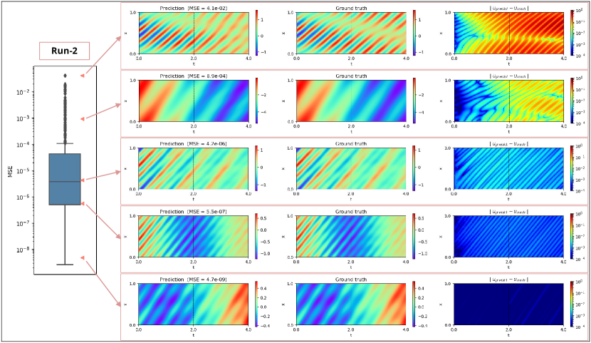
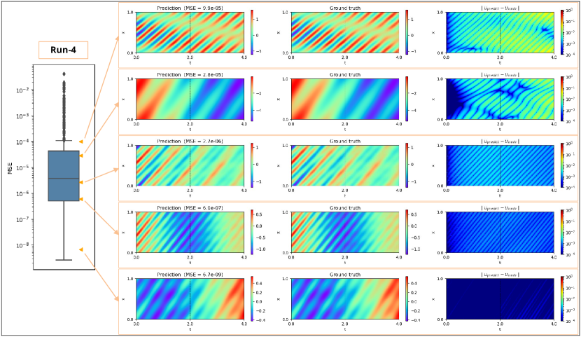
The Baldwinian evolution outcome has the most variation in accuracy across individual runs, on the family of linear PDEs problem relative to the other problems in the experimental studies. The B-PINN MSE results over all test tasks for $t\in[0,4]$ obtained by 5 different runs are 5.3$\mathrm{e}{-5}$ $\pm$1.8$\mathrm{e}{-4}$, 1.7$\mathrm{e}{-5}$ $\pm$3.0$\mathrm{e}{-5}$, 2.0$\mathrm{e}{-3}$ $\pm$5.6$\mathrm{e}{-3}$, 1.5$\mathrm{e}{-3}$ $\pm$3.5$\mathrm{e}{-3}$, and 2.8$\mathrm{e}{-5}$ $\pm$9.1$\mathrm{e}{-5}$, respectively. Figure 8 and 9 compare the solutions of 2 B-PINNs obtained from separate Baldwinian evolution runs, on the same 5 test tasks selected at different levels of accuracy along the MSE spectrum (pooled from $n=87$ test tasks $\times$ 5 individual runs with initial std. = 5).

B.2 Nonlinear PDE problems

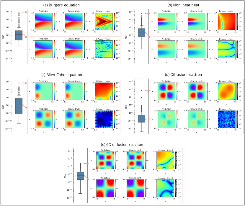
Figure 10 provides additional visualization results for the 5 nonlinear PDE problems described in Section 2.5.2, showing the B-PINN solutions with the worst and median accuracy along the MSE spectrum (pooled from all test tasks $\times$ 5 individual runs) for each problem.

Figure 10: B-PINN solutions with the worst and (approximately) average accuracy along the MSE spectrum (pooled from all test tasks $\times$ 5 individual runs), for 5 nonlinear PDE problems.

B.3 Linear and nonlinear ODEs

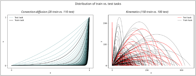
Figure 11 provides additional visualization results for the convection-diffusion and kinematics tasks described in Section 2.4.1, 2.5.1, and 2.6, showing their training and test distributions.

Figure 11: The distribution of convection-diffusion and kinematics tasks for training and test.

References

- \bibcommenthead
- Raissi et al. [2019] Raissi, M., Perdikaris, P., Karniadakis, G.E.: Physics-informed neural networks: A deep learning framework for solving forward and inverse problems involving nonlinear partial differential equations. Journal of Computational physics 378, 686–707 (2019) https://doi.org/10.1016/j.jcp.2018.10.045
- Cuomo et al. [2022] Cuomo, S., Di Cola, V.S., Giampaolo, F., Rozza, G., Raissi, M., Piccialli, F.: Scientific machine learning through physics–informed neural networks: Where we are and what’s next. Journal of Scientific Computing 92(3), 88 (2022) https://doi.org/%****␣sn-article.bbl␣Line␣75␣****10.1007/s10915-022-01939-z
- Karniadakis et al. [2021] Karniadakis, G.E., Kevrekidis, I.G., Lu, L., Perdikaris, P., Wang, S., Yang, L.: Physics-informed machine learning. Nature Reviews Physics 3(6), 422–440 (2021) https://doi.org/10.1038/s42254-021-00314-5
- Raissi et al. [2020] Raissi, M., Yazdani, A., Karniadakis, G.E.: Hidden fluid mechanics: Learning velocity and pressure fields from flow visualizations. Science 367(6481), 1026–1030 (2020)
- Cai et al. [2021a] Cai, S., Mao, Z., Wang, Z., Yin, M., Karniadakis, G.E.: Physics-informed neural networks (pinns) for fluid mechanics: A review. Acta Mechanica Sinica 37(12), 1727–1738 (2021)
- Cai et al. [2021b] Cai, S., Wang, Z., Wang, S., Perdikaris, P., Karniadakis, G.E.: Physics-informed neural networks for heat transfer problems. Journal of Heat Transfer 143(6) (2021)
- Huang and Wang [2022] Huang, B., Wang, J.: Applications of physics-informed neural networks in power systems-a review. IEEE Transactions on Power Systems (2022)
- de Wolff et al. [2021] Wolff, T., Carrillo, H., Martí, L., Sanchez-Pi, N.: Assessing physics informed neural networks in ocean modelling and climate change applications. In: AI: Modeling Oceans and Climate Change Workshop at ICLR 2021 (2021)
- Wong et al. [2022] Wong, J.C., Ooi, C., Gupta, A., Ong, Y.-S.: Learning in sinusoidal spaces with physics-informed neural networks. IEEE Transactions on Artificial Intelligence (2022) https://doi.org/10.1109/TAI.2022.3192362
- Chiu et al. [2022] Chiu, P.-H., Wong, J.C., Ooi, C., Dao, M.H., Ong, Y.-S.: Can-pinn: A fast physics-informed neural network based on coupled-automatic–numerical differentiation method. Computer Methods in Applied Mechanics and Engineering 395, 114909 (2022) https://doi.org/10.1016/j.cma.2022.114909
- Wong et al. [2023] Wong, J.C., Chiu, P.-H., Ooi, C., Dao, M.H., Ong, Y.-S.: Lsa-pinn: Linear boundary connectivity loss for solving pdes on complex geometry. In: 2023 International Joint Conference on Neural Networks (IJCNN), pp. 1–10 (2023). https://doi.org/10.1109/IJCNN54540.2023.10191236
- Wang et al. [2023] Wang, S., Sankaran, S., Wang, H., Perdikaris, P.: An expert’s guide to training physics-informed neural networks. arXiv preprint arXiv:2308.08468 (2023)
- Wong et al. [2021] Wong, J.C., Gupta, A., Ong, Y.-S.: Can transfer neuroevolution tractably solve your differential equations? IEEE Computational Intelligence Magazine 16(2), 14–30 (2021) https://doi.org/10.1109/MCI.2021.3061854
- Krishnapriyan et al. [2021] Krishnapriyan, A., Gholami, A., Zhe, S., Kirby, R., Mahoney, M.W.: Characterizing possible failure modes in physics-informed neural networks. Advances in Neural Information Processing Systems 34, 26548–26560 (2021)
- Penwarden et al. [2023] Penwarden, M., Zhe, S., Narayan, A., Kirby, R.M.: A metalearning approach for physics-informed neural networks (pinns): Application to parameterized pdes. Journal of Computational Physics 477, 111912 (2023) https://doi.org/10.1016/j.jcp.2023.111912
- Downing [2012] Downing, K.L.: Heterochronous neural baldwinism. In: Artificial Life Conference Proceedings, pp. 37–44 (2012). Citeseer
- Simpson [1953] Simpson, G.G.: The baldwin effect. Evolution 7(2), 110–117 (1953)
- Powell [2014] Powell, W.B.: Clearing the jungle of stochastic optimization. In: Bridging Data and Decisions, pp. 109–137. Informs, Catonsville, Maryland, USA (2014)
- Bakker et al. [2020] Bakker, H., Dunke, F., Nickel, S.: A structuring review on multi-stage optimization under uncertainty: Aligning concepts from theory and practice. Omega 96, 102080 (2020)
- Fernando et al. [2018] Fernando, C., Sygnowski, J., Osindero, S., Wang, J., Schaul, T., Teplyashin, D., Sprechmann, P., Pritzel, A., Rusu, A.: Meta-learning by the baldwin effect. In: Proceedings of the Genetic and Evolutionary Computation Conference Companion. GECCO ’18, pp. 1313–1320. Association for Computing Machinery, New York, NY, USA (2018). https://doi.org/10.1145/3205651.3208249 . https://doi.org/10.1145/3205651.3208249
- Stanley et al. [2019] Stanley, K.O., Clune, J., Lehman, J., Miikkulainen, R.: Designing neural networks through neuroevolution. Nature Machine Intelligence 1(1), 24–35 (2019)
- Miikkulainen and Forrest [2021] Miikkulainen, R., Forrest, S.: A biological perspective on evolutionary computation. Nature Machine Intelligence 3(1), 9–15 (2021)
- Hornik et al. [1989] Hornik, K., Stinchcombe, M., White, H.: Multilayer feedforward networks are universal approximators. Neural networks 2(5), 359–366 (1989)
- Chen and Chen [1995] Chen, T., Chen, H.: Universal approximation to nonlinear operators by neural networks with arbitrary activation functions and its application to dynamical systems. IEEE transactions on neural networks 6(4), 911–917 (1995)
- Zhang et al. [2012] Zhang, R., Lan, Y., Huang, G.-b., Xu, Z.-B.: Universal approximation of extreme learning machine with adaptive growth of hidden nodes. IEEE Transactions on Neural Networks and Learning Systems 23(2), 365–371 (2012) https://doi.org/10.1109/TNNLS.2011.2178124
- Dong and Li [2021] Dong, S., Li, Z.: Local extreme learning machines and domain decomposition for solving linear and nonlinear partial differential equations. Computer Methods in Applied Mechanics and Engineering 387, 114129 (2021) https://doi.org/10.1016/j.cma.2021.114129
- Dong and Yang [2022] Dong, S., Yang, J.: On computing the hyperparameter of extreme learning machines: Algorithm and application to computational pdes, and comparison with classical and high-order finite elements. Journal of Computational Physics 463, 111290 (2022) https://doi.org/10.1016/j.jcp.2022.111290
- Gupta and Ong [2018] Gupta, A., Ong, Y.-S.: Memetic Computation: the Mainspring of Knowledge Transfer in a Data-driven Optimization Era vol. 21. Springer, Switzerland (2018)
- Hansen [2016] Hansen, N.: The cma evolution strategy: A tutorial. arXiv preprint arXiv:1604.00772 (2016)
- Bradbury et al. [2018] Bradbury, J., Frostig, R., Hawkins, P., Johnson, M.J., Leary, C., Maclaurin, D., Necula, G., Paszke, A., VanderPlas, J., Wanderman-Milne, S., et al.: Jax: composable transformations of python+ numpy programs (2018)
- Tang et al. [2022] Tang, Y., Tian, Y., Ha, D.: Evojax: Hardware-accelerated neuroevolution. arXiv preprint arXiv:2202.05008 (2022)
- Stynes [2005] Stynes, M.: Steady-state convection-diffusion problems. Acta Numerica 14, 445–508 (2005)
- Van Erp et al. [2020] Van Erp, R., Soleimanzadeh, R., Nela, L., Kampitsis, G., Matioli, E.: Co-designing electronics with microfluidics for more sustainable cooling. Nature 585(7824), 211–216 (2020)
- Patankar [1980] Patankar, S.V.: Numerical Heat Transfer and Fluid Flow. Hemisphere Publishing Corporation, New York, NY, USA (1980)
- Gupta [2013] Gupta, A.: Numerical modelling and optimization of non-isothermal, rigid tool liquid composite moulding processes. PhD thesis, ResearchSpace@ Auckland (2013)
- Bar-Sinai et al. [2019] Bar-Sinai, Y., Hoyer, S., Hickey, J., Brenner, M.P.: Learning data-driven discretizations for partial differential equations. Proceedings of the National Academy of Sciences 116(31), 15344–15349 (2019)
- Brandstetter et al. [2022] Brandstetter, J., Worrall, D., Welling, M.: Message passing neural pde solvers. arXiv preprint arXiv:2202.03376 (2022)
- Bec and Khanin [2007] Bec, J., Khanin, K.: Burgers turbulence. Physics reports 447(1-2), 1–66 (2007)
- Rao et al. [2023] Rao, C., Ren, P., Wang, Q., Buyukozturk, O., Sun, H., Liu, Y.: Encoding physics to learn reaction–diffusion processes. Nature Machine Intelligence 5(7), 765–779 (2023)
- Meng et al. [2020] Meng, X., Li, Z., Zhang, D., Karniadakis, G.E.: Ppinn: Parareal physics-informed neural network for time-dependent pdes. Computer Methods in Applied Mechanics and Engineering 370, 113250 (2020)
- Wang et al. [2022] Wang, S., Sankaran, S., Perdikaris, P.: Respecting causality is all you need for training physics-informed neural networks. arXiv preprint arXiv:2203.07404 (2022)
- Subramanian et al. [2023] Subramanian, S., Harrington, P., Keutzer, K., Bhimji, W., Morozov, D., Mahoney, M., Gholami, A.: Towards foundation models for scientific machine learning: Characterizing scaling and transfer behavior. arXiv preprint arXiv:2306.00258 (2023)
- Suganthan and Katuwal [2021] Suganthan, P.N., Katuwal, R.: On the origins of randomization-based feedforward neural networks. Applied Soft Computing 105, 107239 (2021) https://doi.org/10.1016/j.asoc.2021.107239
- Gallicchio and Scardapane [2020] Gallicchio, C., Scardapane, S.: Deep randomized neural networks. In: Recent Trends in Learning From Data: Tutorials from the INNS Big Data and Deep Learning Conference (INNSBDDL2019), pp. 43–68 (2020). https://doi.org/10.1007/978-3-030-43883-8_3 . Springer
- Baydin et al. [2018] Baydin, A.G., Pearlmutter, B.A., Radul, A.A., Siskind, J.M.: Automatic differentiation in machine learning: a survey. Journal of Marchine Learning Research 18, 1–43 (2018)
- Anderson et al. [2020] Anderson, D., Tannehill, J.C., Pletcher, R.H., Munipalli, R., Shankar, V.: Computational Fluid Mechanics and Heat Transfer. CRC press, Boca Raton, Florida, USA (2020)
- Ollivier et al. [2017] Ollivier, Y., Arnold, L., Auger, A., Hansen, N.: Information-geometric optimization algorithms: A unifying picture via invariance principles. The Journal of Machine Learning Research 18(1), 564–628 (2017)
- Chiu [2018] Chiu, P.-H.: An improved divergence-free-condition compensated method for solving incompressible flows on collocated grids. Computers Fluids 162, 39–54 (2018) https://doi.org/10.1016/j.compfluid.2017.12.005
- Leonard [1991] Leonard, B.P.: The ultimate conservative difference scheme applied to unsteady one-dimensional advection. Computer Methods in Applied Mechanics and Engineering 88, 17–74 (1991) https://doi.org/10.1016/0045-7825(91)90232-U
- Gottlieb and Shu [1998] Gottlieb, S., Shu, C.-W.: Total variation diminishing runge-kutta schemes. Mathematics of Computation 67, 73–85 (1998) https://doi.org/10.1090/S0025-5718-98-00913-2