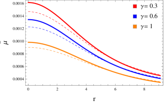
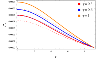
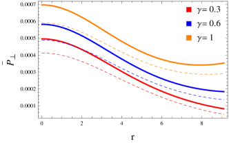
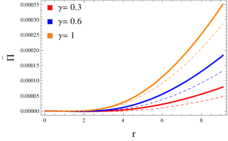
Impact of Charge on Complexity Analysis and Isotropic Decoupled Solutions in fโ€‹(โ„,๐•‹)๐‘“โ„๐•‹f(\mathbb{R},\mathbb{T}) Gravity

M. Sharif1 ย  and Tayyab Naseer1,2
1 Department of Mathematics and Statistics, The University of Lahore,
1-KM Defence Road Lahore-54000, Pakistan.
2 Department of Mathematics, University of the Punjab,
Quaid-i-Azam Campus, Lahore-54590, Pakistan
msharif.math@pu.edu.pktayyabnaseer48@yahoo.com
Abstract

In this paper, we formulate two exact charged solutions to the field equations by extending the domain of existing anisotropic models with the help of minimal gravitational decoupling in fโ€‹(โ„,๐•‹)๐‘“โ„๐•‹f(\mathbb{R},\mathbb{T}) theory. For this, the anisotropic fluid distribution is considered as a seed source that is extended through the inclusion of a new gravitational source. The influence of the later matter configuration is controlled by the decoupling parameter. We formulate the field equations corresponding to the total matter source that are then decoupled into two distinct sets by implementing a transformation only on the radial metric coefficient. Both of these under-determined sets correspond to their parent sources. Some well-behaved forms of the metric potentials are taken into account to deal with the first set of equations. On the other hand, we solve the second set corresponding to an additional source by taking different constraints on the matter sector. We then consider the radius and mass of a compact star 4โ€‹Uโ€‹1820โˆ’304๐‘ˆ1820304U~{}1820-30 to analyze the physical feasibility of the resulting solutions for a particular modified model. It is concluded that our resulting solutions show stable behavior for certain values of the decoupling parameter and charge.

Keywords: fโ€‹(โ„,๐•‹)๐‘“โ„๐•‹f(\mathbb{R},\mathbb{T}) theory; Anisotropy; Self-gravitating systems; Gravitational decoupling.
PACS: 04.50.Kd; 04.40.Dg; 04.40.-b.

1 Introduction

Cosmological breakthroughs show that astrophysical structures are not scattered randomly in our cosmos but are systematically distributed. The analysis of such an integrated paradigm as well as different physical characteristics of compact self-gravitating objects enable astronomers to expose the accelerated expansion of the universe. Multiple modifications to general relativity (๐”พโ€‹โ„๐”พโ„\mathbb{GR}) have been suggested to explain such a cosmic expansion in the recent couple of years. The insertion of the generic function of the Ricci scalar in place of โ„โ„\mathbb{R} in the Einstein-Hilbert action produces the first and straightforward extension of ๐”พโ€‹โ„๐”พโ„\mathbb{GR}, termed the fโ€‹(โ„)๐‘“โ„f(\mathbb{R}) theory. Several researchers made an initial attempt to explain different evolutionary eras of the universe by adopting modified fโ€‹(โ„)๐‘“โ„f(\mathbb{R}) models [1, 2]. The stability of this theory has also been addressed through different techniques [3, 4].

Bertolami et al. [5] initially merged the geometric terms with the matter Lagrangian density in fโ€‹(โ„)๐‘“โ„f(\mathbb{R}) framework to produce the effects of fluid-geometry coupling on the test particles of massive bodies. Several researchers studied such coupling and concluded that it would be advantageous to discuss the cosmic accelerated expansion in this framework. Harko et al. [6] generalized this interaction by introducing a generic function of โ„โ„\mathbb{R} and trace of the energy-momentum tensor (๐”ผโ€‹๐•„โ€‹๐•‹๐”ผ๐•„๐•‹\mathbb{EMT}) ๐•‹๐•‹\mathbb{T} in the action, referred the fโ€‹(โ„,๐•‹)๐‘“โ„๐•‹f(\mathbb{R},\mathbb{T}) theory. The coupling between geometry and matter in this framework provides non-vanishing divergence of the ๐”ผโ€‹๐•„โ€‹๐•‹๐”ผ๐•„๐•‹\mathbb{EMT}. An extra force thus appears in the gravitational field that changes the geodesic motion of the particles under consideration. Different gravitational aspects have been comprised by this theory due to the entanglement of the entity ๐•‹๐•‹\mathbb{T}. Houndjo [7] considered a minimal model of this gravity and explained the transformation of the matter-dominated phase into late-time acceleration era. Das et al. [8] adopted the โ„+2โ€‹ฯ‡3โ€‹๐•‹โ„2subscript๐œ’3๐•‹\mathbb{R}+2\chi_{3}\mathbb{T} model to explore the structure of gravastar comprising three different layers which are expressed by their respective equations of state. Different matter distributions have been discussed for such modified models from which various acceptable solutions representing compact interiors are obtained [9]-[15].

It is worth noting that the problem of the cosmological constant (ฮ›ฮ›\Lambda) can considerably be resolved through a particular choice such as โ„+2โ€‹ฯ‡3โ€‹๐•‹โ„2subscript๐œ’3๐•‹\mathbb{R}+2\chi_{3}\mathbb{T}. It has been shown that the constant ฮ›ฮ›\Lambda can be expressed in proportional relation with the Hubble parameter (โ„=๐šห™๐šโ„ห™๐š๐š\mathbb{H}=\frac{\dot{\mathbf{a}}}{\mathbf{a}}, where ๐š๐š\mathbf{a} denotes the scale factor of the cosmos), i.e., ฮ›eโ€‹fโ€‹fโˆโ„2proportional-tosubscriptฮ›๐‘’๐‘“๐‘“superscriptโ„2\Lambda_{eff}\propto\mathbb{H}^{2} [16]. The second term in the above model is a valid one that could generate several new insights and helps to understand the astronomical structures in a proper way [17, 18]. The model parameter has been restricted as ฯ‡3>โˆ’3.0ร—10โˆ’4subscript๐œ’33.0superscript104\chi_{3}>-3.0\times 10^{-4} while studying massive white dwarfs [19]. In addition, the background evolution provided a limit on this parameter as โˆ’0.1<ฯ‡3<1.50.1subscript๐œ’31.5-0.1<\chi_{3}<1.5 [20]. Also, the lower bound of ฯ‡3subscript๐œ’3\chi_{3} was obtained as โˆ’1.9ร—10โˆ’81.9superscript108-1.9\times 10^{-8} from the dark energy density parameter [21]. Ashmita et al. [22] adopted three different inflation potentials in this modified theory, and derived the corresponding field equations and potential slow-roll parameters. They concluded that their results are compatible with the observational data only for โˆ’0.37<ฯ‡3<1.4830.37subscript๐œ’31.483-0.37<\chi_{3}<1.483. Kaur et al. [23] assumed this model to discuss the interior of charged anisotropic Tolman-Kuchowicz solution and found it stable as well as viable.

The nature of compact stellar bodies in our universe can be understood by formulating the solutions (exact or numerical) of their respective field equations. The highly non-linear nature of such equations prompted several astrophysicists to find different techniques so that these equations can be solved easily which further helps to check the physical relevancy of the respective model. One of the multiple approaches discussed in the literature is the gravitational decoupling that helps to obtain the feasible solution of the interior fluid distribution possessing multiple factors like pressure anisotropy, heat dissipation and shear stress. This approach solves the field equations corresponding to more than one matter configuration by transforming the metric components to a new frame of reference which makes much easier to solve them. Gravitational decoupling offers two schemes, one of them is the minimal geometric deformation (MGD). Ovalle [24] recently developed this approach and found the analytic solutions representing stellar objects in the braneworld (BW). Later, Ovalle and Linares [25] formulated an exact solution to the field equations for an isotropic sphere by using the MGD technique along with the Tolman-IV metric potentials in the BW scenario. Casadio et al. [26] developed a consistent extension of the above technique and proposed a new solution in the context of BW that helps to discuss the geometry of stars.

Ovalle et al. [27] employed the gravitational decoupling through MGD approach and extended an isotropic solution to the anisotropic domain. They also analyzed the feasibility of resulting solutions through graphical interpretation. These isotropic solutions were then extended to the case of charged Krori-Barua anisotropic sphere in which the influence of an electromagnetic field on the stability of resulting models has been checked [28]. Gabbanelli et al. [29] developed the anisotropic Duragpal-Fuloria models representing physically relevant celestial objects. The same analysis has also been done for multiple extensions of the isotropic Heintzmann as well as Tolman VII spacetimes [30, 31]. The MGD approach was also used to extend several isotropic spacetimes to an acceptable anisotropic domain in Brans-Dicke theory [32]. Multiple compact models have been developed in a non-minimal gravitational theory through the decoupling technique [33]. The influence of the respective parameter was also checked on the corresponding physical determinants.

The analysis of self-gravitating celestial systems has been observed to be significantly affected by the presence of an electric charge. A strongly attractive nature of gravity can be reduced or counterbalanced through some important ingredients, one of them is the electromagnetic force. For this reason, a compact body needs a sufficient amount of the charge in order to resist the gravitational attraction and preserve its stable state. This has been confirmed by Bekenstein [34] while studying a charged dynamical sphere. He concluded that the nature of the electromagnetic force is opposite to that of gravity, helping the considered geometry to be stable. Esculpi and Aloma [35] have extended this work to explore the behavior of anisotropic matter distribution in a compact interior. They observed that the spacetime experiences a repulsive force due to the presence of both charge and positive anisotropy. Some anisotropic charged compact stars have been studied by adopting a particular form of the interior charge in terms of the spherical radius and acceptable results were obtained [36, 37]. Pretel et al. [38] explored the interior distribution of charged quark stars through a linear equation of state in the context of โ„+2โ€‹ฯ‡3โ€‹๐•‹โ„2subscript๐œ’3๐•‹\mathbb{R}+2\chi_{3}\mathbb{T} gravity. They observed that the parameters measuring the impact of charge and modified theory considerably affect the total mass and radius of the star. Several physically relevant charged compact stars have been modeled by us in a non-minimally coupled framework [39].

Herrera [40] suggested a very recent definition of the complexity for static self-gravitation spherical systems. He used Belโ€™s idea for the orthogonal decomposition of the curvature tensor corresponding to the anisotropic matter configuration and found several scalars. It was then observed that there is only one scalar that involves the inhomogeneous density and anisotropy, thus referred as the complexity factor. This definition becomes widely accepted for the last couple of years in the scientific community. Herrera with his collaborators also extended this definition for dynamical matter source [41]. Such extensions have been developed in non-minimally coupled theory for static/non-static spherical and cylindrical interiors [42, 43]. Different constraints have been used in the literature to make the system solvable. Several researchers [44] used the complexity-free condition as a constraint and merged it with the decoupling strategy to obtain physically relevant stellar models. Casadio et al. [45] considered anisotropic compact model and isotropized it by varying the decoupling parameter involving in the MGD technique. Maurya et al. [46] adopted the no complexity constraint and checked the effect of the decoupling parameter on the developed embedding class-one model. Sharif and Majid [47] also formulated such models in Brans-Dicke theory and found them stable for certain parametric values.

In this article, we investigate how two different solutions representing compact models are affected by the charge as well as modified corrections of fโ€‹(โ„,๐•‹)๐‘“โ„๐•‹f(\mathbb{R},\mathbb{T}) gravity. Following lines depict how this paper is organized. We introduce some basic foundations of the modified theory and formulate the corresponding field equations in the presence of charge as well as an extra matter source in section 2. Section 3 separates these equations into two sets through the MGD scheme. Two different constraints depending on the matter sector are adopted in sections 4 and 5, leading to the resulting solutions. Section 6 analyzes the corresponding matter determinants and other physical characteristics to check whether the modified models are physically relevant or not. Lastly, section 7 sums up our results.

2 fโ€‹(โ„,๐•‹)๐‘“โ„๐•‹f(\mathbb{R},\mathbb{T}) Gravity

The presence of an additional source in the gravitational field modifies the Einstein-Hilbert action (with ฮบ=8โ€‹ฯ€๐œ…8๐œ‹\kappa=8\pi) in the following form [6]

S=โˆซโˆ’gโ€‹[fโ€‹(โ„,๐•‹)16โ€‹ฯ€+๐•ƒm+๐•ƒ๐”ผ+ฮณโ€‹๐•ƒโ„ญ]โ€‹d4โ€‹x,S๐‘”delimited-[]๐‘“โ„๐•‹16๐œ‹subscript๐•ƒ๐‘šsubscript๐•ƒ๐”ผ๐›พsubscript๐•ƒโ„ญsuperscript๐‘‘4๐‘ฅ\mathrm{S}=\int\sqrt{-g}\left[\frac{f(\mathbb{R},\mathbb{T})}{16\pi}+\mathbb{L}_{m}+\mathbb{L}_{\mathbb{E}}+\gamma\mathbb{L}_{\mathfrak{C}}\right]d^{4}x, (1)

where ๐•ƒโ„ญsubscript๐•ƒโ„ญ\mathbb{L}_{\mathfrak{C}} being the Lagrangian density of an extra source gravitationally coupled to the original field, ๐•ƒmsubscript๐•ƒ๐‘š\mathbb{L}_{m} and ๐•ƒ๐”ผsubscript๐•ƒ๐”ผ\mathbb{L}_{\mathbb{E}} are that of the matter distribution and an electromagnetic field, respectively. Also, the determinant of the metric tensor gฮฒโ€‹ฮฑsubscript๐‘”๐›ฝ๐›ผg_{\beta\alpha} is symbolized by g๐‘”g. Taking the action (1) and applying the principle of least-action produces the field equations as

๐”พฮฒโ€‹ฮฑ=8โ€‹ฯ€โ€‹๐•‹ฮฒโ€‹ฮฑ(total),subscript๐”พ๐›ฝ๐›ผ8๐œ‹superscriptsubscript๐•‹๐›ฝ๐›ผtotal\mathbb{G}_{\beta\alpha}=8\pi\mathbb{T}_{\beta\alpha}^{(\mathrm{total})}, (2)

where ๐”พฮฒโ€‹ฮฑsubscript๐”พ๐›ฝ๐›ผ\mathbb{G}_{\beta\alpha} being an Einstein tensor that describes the geometry of the spacetime whereas the interior fluid distribution is characterized by the right hand side of the above equation. We further classify it for the current scenario as

๐•‹ฮฒโ€‹ฮฑ(total)=๐•‹ฮฒโ€‹ฮฑ(ef)+ฮณโ€‹โ„ญฮฒโ€‹ฮฑ=1fโ„โ€‹(๐•‹ฮฒโ€‹ฮฑ+๐”ผฮฒโ€‹ฮฑ)+๐•‹ฮฒโ€‹ฮฑ(D)+ฮณโ€‹โ„ญฮฒโ€‹ฮฑ,superscriptsubscript๐•‹๐›ฝ๐›ผtotalsuperscriptsubscript๐•‹๐›ฝ๐›ผef๐›พsubscriptโ„ญ๐›ฝ๐›ผ1subscript๐‘“โ„subscript๐•‹๐›ฝ๐›ผsubscript๐”ผ๐›ฝ๐›ผsuperscriptsubscript๐•‹๐›ฝ๐›ผD๐›พsubscriptโ„ญ๐›ฝ๐›ผ\mathbb{T}_{\beta\alpha}^{(\mathrm{total})}=\mathbb{T}_{\beta\alpha}^{(\mathrm{ef})}+\gamma\mathfrak{C}_{\beta\alpha}=\frac{1}{f_{\mathbb{R}}}\big{(}\mathbb{T}_{\beta\alpha}+\mathbb{E}_{\beta\alpha}\big{)}+\mathbb{T}_{\beta\alpha}^{(\mathrm{D})}+\gamma\mathfrak{C}_{\beta\alpha}, (3)

where fโ„=โˆ‚fโ€‹(โ„,๐•‹)โˆ‚โ„subscript๐‘“โ„๐‘“โ„๐•‹โ„f_{\mathbb{R}}=\frac{\partial f(\mathbb{R},\mathbb{T})}{\partial\mathbb{R}}. Moreover, ฮณ๐›พ\gamma controls the effect of an additional matter sector (โ„ญฮฒโ€‹ฮฑsubscriptโ„ญ๐›ฝ๐›ผ\mathfrak{C}_{\beta\alpha}) on the seed interior configuration of celestial systems, and we call it the decoupling parameter. The modification in the Einstein-Hilbert action results in the effective ๐”ผโ€‹๐•„โ€‹๐•‹๐”ผ๐•„๐•‹\mathbb{EMT}, denoted by ๐•‹ฮฒโ€‹ฮฑ(ef)superscriptsubscript๐•‹๐›ฝ๐›ผef\mathbb{T}_{\beta\alpha}^{(\mathrm{ef})} containing the usual matter part of ๐”พโ€‹โ„๐”พโ„\mathbb{GR} (in which ๐•‹ฮฒโ€‹ฮฑsubscript๐•‹๐›ฝ๐›ผ\mathbb{T}_{\beta\alpha} and ๐”ผฮฒโ€‹ฮฑsubscript๐”ผ๐›ฝ๐›ผ\mathbb{E}_{\beta\alpha} being the usual and electromagnetic ๐”ผโ€‹๐•„โ€‹๐•‹โ€‹s๐”ผ๐•„๐•‹๐‘ \mathbb{EMT}s, respectively) and correction terms ๐•‹ฮฒโ€‹ฮฑ(D)superscriptsubscript๐•‹๐›ฝ๐›ผD\mathbb{T}_{\beta\alpha}^{(\mathrm{D})} of the extended theory. The later term has the form

๐•‹ฮฒโ€‹ฮฑ(D)superscriptsubscript๐•‹๐›ฝ๐›ผD\displaystyle\mathbb{T}_{\beta\alpha}^{(\mathrm{D})} =\displaystyle= 18โ€‹ฯ€โ€‹fโ„[๐•‹ฮฒโ€‹ฮฑf๐•‹+{12(fโˆ’โ„fโ„)โˆ’๐•ƒmf๐•‹}gฮฒโ€‹ฮฑ\displaystyle\frac{1}{8\pi f_{\mathbb{R}}}\bigg{[}\mathbb{T}_{\beta\alpha}f_{\mathbb{T}}+\bigg{\{}\frac{1}{2}\big{(}f-\mathbb{R}f_{\mathbb{R}}\big{)}-\mathbb{L}_{m}f_{\mathbb{T}}\bigg{\}}g_{\beta\alpha} (4)
โˆ’\displaystyle- (gฮฒโ€‹ฮฑโ–กโˆ’โˆ‡ฮฒโˆ‡ฮฑ)fโ„+2gฯโ€‹ฮถf๐•‹โˆ‚2๐•ƒmโˆ‚gฮฒโ€‹ฮฑโ€‹โˆ‚gฯโ€‹ฮถ],\displaystyle(g_{\beta\alpha}\Box-\nabla_{\beta}\nabla_{\alpha})f_{\mathbb{R}}+2g^{\rho\zeta}f_{\mathbb{T}}\frac{\partial^{2}\mathbb{L}_{m}}{\partial g^{\beta\alpha}\partial g^{\rho\zeta}}\bigg{]},

where f๐•‹=โˆ‚fโ€‹(โ„,๐•‹)โˆ‚๐•‹subscript๐‘“๐•‹๐‘“โ„๐•‹๐•‹f_{\mathbb{T}}=\frac{\partial f(\mathbb{R},\mathbb{T})}{\partial\mathbb{T}}. Also, the term โˆ‡ฮฒsubscriptโˆ‡๐›ฝ\nabla_{\beta} being the covariant derivative and โ–กโ‰ก1โˆ’gโ€‹โˆ‚ฮฒ(โˆ’gโ€‹gฮฒโ€‹ฮฑโ€‹โˆ‚ฮฑ)โ–ก1๐‘”subscript๐›ฝ๐‘”superscript๐‘”๐›ฝ๐›ผsubscript๐›ผ\Box\equiv\frac{1}{\sqrt{-g}}\partial_{\beta}\big{(}\sqrt{-g}g^{\beta\alpha}\partial_{\alpha}\big{)} is the Dโ€™Alembertian operator.

We shall discuss the complexity of a self-gravitating system, therefore, the nature of seed fluid distribution must be anisotropic. The following ๐”ผโ€‹๐•„โ€‹๐•‹๐”ผ๐•„๐•‹\mathbb{EMT} represents such kind of fluids as

๐•‹ฮฒโ€‹ฮฑ=ฮผโ€‹๐’ฆฮฒโ€‹๐’ฆฮฑ+PโŠฅโ€‹(๐’ฆฮฒโ€‹๐’ฆฮฑ+gฮฒโ€‹ฮฑโˆ’๐’ฒฮฒโ€‹๐’ฒฮฑ)+Prโ€‹๐’ฒฮฒโ€‹๐’ฒฮฑ,subscript๐•‹๐›ฝ๐›ผ๐œ‡subscript๐’ฆ๐›ฝsubscript๐’ฆ๐›ผsubscript๐‘ƒbottomsubscript๐’ฆ๐›ฝsubscript๐’ฆ๐›ผsubscript๐‘”๐›ฝ๐›ผsubscript๐’ฒ๐›ฝsubscript๐’ฒ๐›ผsubscript๐‘ƒ๐‘Ÿsubscript๐’ฒ๐›ฝsubscript๐’ฒ๐›ผ\mathbb{T}_{\beta\alpha}=\mu\mathcal{K}_{\beta}\mathcal{K}_{\alpha}+P_{\bot}\big{(}\mathcal{K}_{\beta}\mathcal{K}_{\alpha}+g_{\beta\alpha}-\mathcal{W}_{\beta}\mathcal{W}_{\alpha}\big{)}+P_{r}\mathcal{W}_{\beta}\mathcal{W}_{\alpha}, (5)

where the triplet (Pr,PโŠฅ,ฮผsubscript๐‘ƒ๐‘Ÿsubscript๐‘ƒbottom๐œ‡P_{r},P_{\bot},\mu) symbolizes the radial/tangential pressure and density, respectively. Further, ๐’ฆฮฒsubscript๐’ฆ๐›ฝ\mathcal{K}_{\beta} being the four-velocity and ๐’ฒฮฒsubscript๐’ฒ๐›ฝ\mathcal{W}_{\beta} is the four-vector satisfying the following relations

๐’ฒฮฒโ€‹๐’ฆฮฒ=0,๐’ฒฮฒโ€‹๐’ฒฮฒ=1,๐’ฆฮฒโ€‹๐’ฆฮฒ=โˆ’1.formulae-sequencesuperscript๐’ฒ๐›ฝsubscript๐’ฆ๐›ฝ0formulae-sequencesuperscript๐’ฒ๐›ฝsubscript๐’ฒ๐›ฝ1superscript๐’ฆ๐›ฝsubscript๐’ฆ๐›ฝ1\mathcal{W}^{\beta}\mathcal{K}_{\beta}=0,\quad\mathcal{W}^{\beta}\mathcal{W}_{\beta}=1,\quad\mathcal{K}^{\beta}\mathcal{K}_{\beta}=-1.

Further, the expression for ๐”ผฮฒโ€‹ฮฑsubscript๐”ผ๐›ฝ๐›ผ\mathbb{E}_{\beta\alpha} is provided by

๐”ผฮฒโ€‹ฮฑ=โˆ’14โ€‹ฯ€โ€‹[14โ€‹gฮฒโ€‹ฮฑโ€‹๐”ฝฮถโ€‹ฮทโ€‹๐”ฝฮถโ€‹ฮทโˆ’๐”ฝฮฒฮถโ€‹๐”ฝฮฑโ€‹ฮถ].subscript๐”ผ๐›ฝ๐›ผ14๐œ‹delimited-[]14subscript๐‘”๐›ฝ๐›ผsuperscript๐”ฝ๐œ๐œ‚subscript๐”ฝ๐œ๐œ‚subscriptsuperscript๐”ฝ๐œ๐›ฝsubscript๐”ฝ๐›ผ๐œ\mathbb{E}_{\beta\alpha}=-\frac{1}{4\pi}\left[\frac{1}{4}g_{\beta\alpha}\mathbb{F}^{\zeta\eta}\mathbb{F}_{\zeta\eta}-\mathbb{F}^{\zeta}_{\beta}\mathbb{F}_{\alpha\zeta}\right].

Here, the Maxwell field tensor is defined as ๐”ฝฮถโ€‹ฮท=ฮฆฮท;ฮถโˆ’ฮฆฮถ;ฮทsubscript๐”ฝ๐œ๐œ‚subscriptฮฆ๐œ‚๐œsubscriptฮฆ๐œ๐œ‚\mathbb{F}_{\zeta\eta}=\Phi_{\eta;\zeta}-\Phi_{\zeta;\eta} with ฮฆฮถ=ฮฆโ€‹(r)โ€‹ฮดฮถ0subscriptฮฆ๐œฮฆ๐‘Ÿsubscriptsuperscript๐›ฟ0๐œ\Phi_{\zeta}=\Phi(r)\delta^{0}_{\zeta} being the four-potential. A concise form of the Maxwell equations is presented in the following

๐”ฝ;ฮทฮถโ€‹ฮท=4โ€‹ฯ€โ€‹ศทฮถ,๐”ฝ[ฮถโ€‹ฮท;ฮฑ]=0,\mathbb{F}^{\zeta\eta}_{;\eta}=4\pi\jmath^{\zeta},\quad\mathbb{F}_{[\zeta\eta;\alpha]}=0, (6)

where ศทฮถ=ฮฉโ€‹๐’ฆฮถsuperscriptitalic-ศท๐œฮฉsuperscript๐’ฆ๐œ\jmath^{\zeta}=\Omega\mathcal{K}^{\zeta} and ฮฉฮฉ\Omega being the current and charge densities, respectively.

The extended field equations (2) have the following trace given by

(โ„+3โ€‹โˆ‡ฮฒโˆ‡ฮฒ)โ€‹fโ„โˆ’๐•‹+(๐•‹+4โ€‹๐•ƒm)โ€‹f๐•‹โˆ’2โ€‹fโˆ’2โ€‹f๐•‹โ€‹gฯโ€‹ฮถโ€‹gฮฒโ€‹ฮฑโ€‹โˆ‚2๐•ƒmโˆ‚gฯโ€‹ฮถโ€‹โˆ‚gฮฒโ€‹ฮฑ=0.โ„3superscriptโˆ‡๐›ฝsubscriptโˆ‡๐›ฝsubscript๐‘“โ„๐•‹๐•‹4subscript๐•ƒ๐‘šsubscript๐‘“๐•‹2๐‘“2subscript๐‘“๐•‹superscript๐‘”๐œŒ๐œsuperscript๐‘”๐›ฝ๐›ผsuperscript2subscript๐•ƒ๐‘šsuperscript๐‘”๐œŒ๐œsuperscript๐‘”๐›ฝ๐›ผ0\displaystyle\big{(}\mathbb{R}+3\nabla^{\beta}\nabla_{\beta}\big{)}f_{\mathbb{R}}-\mathbb{T}+\big{(}\mathbb{T}+4\mathbb{L}_{m}\big{)}f_{\mathbb{T}}-2f-2f_{\mathbb{T}}g^{\rho\zeta}g^{\beta\alpha}\frac{\partial^{2}\mathbb{L}_{m}}{\partial g^{\rho\zeta}\partial g^{\beta\alpha}}=0.

By taking the vacuum case into account, we can retrieve the fโ€‹(โ„,๐•‹)๐‘“โ„๐•‹f(\mathbb{R},\mathbb{T}) equations of motion and their solutions to fโ€‹(โ„)๐‘“โ„f(\mathbb{R}) gravitational theory. The covariant divergence of effective ๐”ผโ€‹๐•„โ€‹๐•‹๐”ผ๐•„๐•‹\mathbb{EMT} is zero, however, that of usual matter distribution is non-null due to the inclusion of the curvature-matter coupling in the gravitational action. Consequently, an additional force comes into existence that can be seen from the following expression

โˆ‡ฮฒ๐•‹ฮฒโ€‹ฮฑsuperscriptโˆ‡๐›ฝsubscript๐•‹๐›ฝ๐›ผ\displaystyle\nabla^{\beta}\mathbb{T}_{\beta\alpha} =f๐•‹8โ€‹ฯ€โˆ’f๐•‹[(๐•‹ฮฒโ€‹ฮฑ+ฮ˜ฮฒโ€‹ฮฑ)โˆ‡ฮฒlnf๐•‹+โˆ‡ฮฒฮ˜ฮฒโ€‹ฮฑ\displaystyle=\frac{f_{\mathbb{T}}}{8\pi-f_{\mathbb{T}}}\bigg{[}(\mathbb{T}_{\beta\alpha}+\Theta_{\beta\alpha})\nabla^{\beta}\ln{f_{\mathbb{T}}}+\nabla^{\beta}\Theta_{\beta\alpha}
โˆ’8โ€‹ฯ€โ€‹ฮณf๐•‹โˆ‡ฮฒโ„ญฮฒโ€‹ฮฑโˆ’12gฯโ€‹ฮถโˆ‡ฮฑ๐•‹ฯโ€‹ฮถโˆ’8โ€‹ฯ€f๐•‹โˆ‡ฮฒ๐”ผฮฒโ€‹ฮฑ],\displaystyle-\frac{8\pi\gamma}{f_{\mathbb{T}}}\nabla^{\beta}\mathfrak{C}_{\beta\alpha}-\frac{1}{2}g_{\rho\zeta}\nabla_{\alpha}\mathbb{T}^{\rho\zeta}-\frac{8\pi}{f_{\mathbb{T}}}\nabla^{\beta}\mathbb{E}_{\beta\alpha}\bigg{]}, (7)

where ฮ˜ฮฒโ€‹ฮฑ=gฮฒโ€‹ฮฑโ€‹๐•ƒmโˆ’2โ€‹๐•‹ฮฒโ€‹ฮฑโˆ’2โ€‹gฯโ€‹ฮถโ€‹โˆ‚2๐•ƒmโˆ‚gฮฒโ€‹ฮฑโ€‹โˆ‚gฯโ€‹ฮถsubscriptฮ˜๐›ฝ๐›ผsubscript๐‘”๐›ฝ๐›ผsubscript๐•ƒ๐‘š2subscript๐•‹๐›ฝ๐›ผ2superscript๐‘”๐œŒ๐œsuperscript2subscript๐•ƒ๐‘šsuperscript๐‘”๐›ฝ๐›ผsuperscript๐‘”๐œŒ๐œ\Theta_{\beta\alpha}=g_{\beta\alpha}\mathbb{L}_{m}-2\mathbb{T}_{\beta\alpha}-2g^{\rho\zeta}\frac{\partial^{2}\mathbb{L}_{m}}{\partial g^{\beta\alpha}\partial g^{\rho\zeta}}. Several choices of the matter Lagrangian have been analyzed in the literature for isotropic/anisotropic fluids including the energy density, pressure, torsion, etc. Since we consider the anisotropic matter distribution, ๐•ƒm=P=2โ€‹PโŠฅ+Pr3subscript๐•ƒ๐‘š๐‘ƒ2subscript๐‘ƒbottomsubscript๐‘ƒ๐‘Ÿ3\mathbb{L}_{m}=P=\frac{2P_{\bot}+P_{r}}{3} is the most suitable choice in this case [6].

A self-gravitating geometry can be distinguished into an interior and exterior regions by the hypersurface ฮฃฮฃ\Sigma. We define the interior region of a static spherical spacetime by the following line element as

ds2=โˆ’eฯ‡1โ€‹dโ€‹t2+eฯ‡2โ€‹dโ€‹r2+r2โ€‹dโ€‹ฯ‘2+r2โ€‹sin2โกฯ‘โ€‹dโ€‹ฯ†2,superscriptds2superscript๐‘’subscript๐œ’1๐‘‘superscript๐‘ก2superscript๐‘’subscript๐œ’2๐‘‘superscript๐‘Ÿ2superscript๐‘Ÿ2๐‘‘superscriptitalic-ฯ‘2superscript๐‘Ÿ2superscript2italic-ฯ‘๐‘‘superscript๐œ‘2\mathrm{ds}^{2}=-e^{\chi_{1}}dt^{2}+e^{\chi_{2}}dr^{2}+r^{2}d\vartheta^{2}+r^{2}\sin^{2}\vartheta d\varphi^{2}, (8)

where ฯ‡1=ฯ‡1โ€‹(r)subscript๐œ’1subscript๐œ’1๐‘Ÿ\chi_{1}=\chi_{1}(r) and ฯ‡2=ฯ‡2โ€‹(r)subscript๐œ’2subscript๐œ’2๐‘Ÿ\chi_{2}=\chi_{2}(r). The two quantities ๐’ฒฮฒsubscript๐’ฒ๐›ฝ\mathcal{W}_{\beta} and ๐’ฆฮฒsubscript๐’ฆ๐›ฝ\mathcal{K}_{\beta} in Eq.(5) become in terms of the above metric as

๐’ฒฮฒ=(0,eฯ‡22,0,0),๐’ฆฮฒ=(โˆ’eฯ‡12,0,0,0).formulae-sequencesubscript๐’ฒ๐›ฝ0superscript๐‘’subscript๐œ’2200subscript๐’ฆ๐›ฝsuperscript๐‘’subscript๐œ’12000\mathcal{W}_{\beta}=(0,e^{\frac{\chi_{2}}{2}},0,0),\quad\mathcal{K}_{\beta}=(-e^{\frac{\chi_{1}}{2}},0,0,0).

Further, Eq.(6) (left) now leads to the following differential equation

ฮฆโ€ฒโ€ฒโˆ’12โ€‹rโ€‹{rโ€‹(ฯ‡1โ€ฒ+ฯ‡2โ€ฒ)โˆ’4}โ€‹ฮฆโ€ฒ=4โ€‹ฯ€โ€‹ฮฉโ€‹eฯ‡12+ฯ‡2,superscriptฮฆโ€ฒโ€ฒ12๐‘Ÿ๐‘Ÿsuperscriptsubscript๐œ’1โ€ฒsuperscriptsubscript๐œ’2โ€ฒ4superscriptฮฆโ€ฒ4๐œ‹ฮฉsuperscript๐‘’subscript๐œ’12subscript๐œ’2\Phi^{\prime\prime}-\frac{1}{2r}\big{\{}r(\chi_{1}^{\prime}+\chi_{2}^{\prime})-4\big{\}}\Phi^{\prime}=4\pi\Omega e^{\frac{\chi_{1}}{2}+\chi_{2}}, (9)

whose integration yields

ฮฆโ€ฒ=sโ€‹(r)r2โ€‹eฯ‡1+ฯ‡22,superscriptฮฆโ€ฒs๐‘Ÿsuperscript๐‘Ÿ2superscript๐‘’subscript๐œ’1subscript๐œ’22\Phi^{\prime}=\frac{\mathrm{s}(r)}{r^{2}}e^{\frac{\chi_{1}+\chi_{2}}{2}}, (10)

where =โ€ฒโˆ‚โˆ‚r{}^{\prime}=\frac{\partial}{\partial r} and sโ€‹(r)=โˆซ0rฮฉโ€‹eฯ‡22โ€‹r^2โ€‹๐‘‘r^s๐‘Ÿsuperscriptsubscript0๐‘Ÿฮฉsuperscript๐‘’subscript๐œ’22superscript^๐‘Ÿ2differential-d^๐‘Ÿ\mathrm{s}(r)=\int_{0}^{r}\Omega e^{\frac{\chi_{2}}{2}}\hat{r}^{2}d\hat{r} being the total interior charge.

We shall present a graphical analysis of the resulting solutions (will be developed in the later sections), thus it is necessary to adopt a specific model that can help us to express our results meaningfully. Several matter-geometry coupled fโ€‹(โ„,๐•‹)๐‘“โ„๐•‹f(\mathbb{R},\mathbb{T}) models have been studied in the literature. Since we aim to find our solutions through the gravitational decoupling strategy, a very useful linear model in this regard is assumed in the following

fโ€‹(โ„,๐•‹)=f1โ€‹(โ„)+f2โ€‹(๐•‹)=โ„+2โ€‹ฯ‡3โ€‹๐•‹,๐‘“โ„๐•‹subscript๐‘“1โ„subscript๐‘“2๐•‹โ„2subscript๐œ’3๐•‹f(\mathbb{R},\mathbb{T})=f_{1}(\mathbb{R})+f_{2}(\mathbb{T})=\mathbb{R}+2\chi_{3}\mathbb{T}, (11)

where ๐•‹=Pr+2โ€‹PโŠฅโˆ’ฮผ๐•‹subscript๐‘ƒ๐‘Ÿ2subscript๐‘ƒbottom๐œ‡\mathbb{T}=P_{r}+2P_{\bot}-\mu and ฯ‡3subscript๐œ’3\chi_{3} being a real-valued coupling constant. We have employed this model to construct two different anisotropic solutions and observed our results consistent with ๐”พโ€‹โ„๐”พโ„\mathbb{GR} [48].

The line element (8) and modified model (11) produce the non-zero components of the field equations (2) as

8โ€‹ฯ€โ€‹(ฮผโˆ’ฮณโ€‹โ„ญ00)+s2r48๐œ‹๐œ‡๐›พsuperscriptsubscriptโ„ญ00superscripts2superscript๐‘Ÿ4\displaystyle 8\pi\left(\mu-\gamma\mathfrak{C}_{0}^{0}\right)+\frac{\mathrm{s}^{2}}{r^{4}} =eโˆ’ฯ‡2โ€‹(ฯ‡2โ€ฒrโˆ’1r2)+1r2โˆ’ฯ‡3โ€‹(3โ€‹ฮผโˆ’Pr3โˆ’2โ€‹PโŠฅ3),absentsuperscript๐‘’subscript๐œ’2superscriptsubscript๐œ’2โ€ฒ๐‘Ÿ1superscript๐‘Ÿ21superscript๐‘Ÿ2subscript๐œ’33๐œ‡subscript๐‘ƒ๐‘Ÿ32subscript๐‘ƒbottom3\displaystyle=e^{-\chi_{2}}\bigg{(}\frac{\chi_{2}^{\prime}}{r}-\frac{1}{r^{2}}\bigg{)}+\frac{1}{r^{2}}-\chi_{3}\bigg{(}3\mu-\frac{P_{r}}{3}-\frac{2P_{\bot}}{3}\bigg{)}, (12)
8โ€‹ฯ€โ€‹(Pr+ฮณโ€‹โ„ญ11)โˆ’s2r48๐œ‹subscript๐‘ƒ๐‘Ÿ๐›พsuperscriptsubscriptโ„ญ11superscripts2superscript๐‘Ÿ4\displaystyle 8\pi\left(P_{r}+\gamma\mathfrak{C}_{1}^{1}\right)-\frac{\mathrm{s}^{2}}{r^{4}} =eโˆ’ฯ‡2โ€‹(1r2+ฯ‡1โ€ฒr)โˆ’1r2+ฯ‡3โ€‹(ฮผโˆ’7โ€‹Pr3โˆ’2โ€‹PโŠฅ3),absentsuperscript๐‘’subscript๐œ’21superscript๐‘Ÿ2superscriptsubscript๐œ’1โ€ฒ๐‘Ÿ1superscript๐‘Ÿ2subscript๐œ’3๐œ‡7subscript๐‘ƒ๐‘Ÿ32subscript๐‘ƒbottom3\displaystyle=e^{-\chi_{2}}\bigg{(}\frac{1}{r^{2}}+\frac{\chi_{1}^{\prime}}{r}\bigg{)}-\frac{1}{r^{2}}+\chi_{3}\bigg{(}\mu-\frac{7P_{r}}{3}-\frac{2P_{\bot}}{3}\bigg{)}, (13)
8โ€‹ฯ€โ€‹(PโŠฅ+ฮณโ€‹โ„ญ22)+s2r48๐œ‹subscript๐‘ƒbottom๐›พsuperscriptsubscriptโ„ญ22superscripts2superscript๐‘Ÿ4\displaystyle 8\pi\left(P_{\bot}+\gamma\mathfrak{C}_{2}^{2}\right)+\frac{\mathrm{s}^{2}}{r^{4}} =eโˆ’ฯ‡24โ€‹(ฯ‡1โ€ฒโฃ2โˆ’ฯ‡2โ€ฒโ€‹ฯ‡1โ€ฒ+2โ€‹ฯ‡1โ€ฒโ€ฒโˆ’2โ€‹ฯ‡2โ€ฒr+2โ€‹ฯ‡1โ€ฒr)absentsuperscript๐‘’subscript๐œ’24superscriptsubscript๐œ’1โ€ฒ2superscriptsubscript๐œ’2โ€ฒsuperscriptsubscript๐œ’1โ€ฒ2superscriptsubscript๐œ’1โ€ฒโ€ฒ2superscriptsubscript๐œ’2โ€ฒ๐‘Ÿ2superscriptsubscript๐œ’1โ€ฒ๐‘Ÿ\displaystyle=\frac{e^{-\chi_{2}}}{4}\bigg{(}\chi_{1}^{\prime 2}-\chi_{2}^{\prime}\chi_{1}^{\prime}+2\chi_{1}^{\prime\prime}-\frac{2\chi_{2}^{\prime}}{r}+\frac{2\chi_{1}^{\prime}}{r}\bigg{)}
+ฯ‡3โ€‹(ฮผโˆ’Pr3โˆ’8โ€‹PโŠฅ3),subscript๐œ’3๐œ‡subscript๐‘ƒ๐‘Ÿ38subscript๐‘ƒbottom3\displaystyle+\chi_{3}\bigg{(}\mu-\frac{P_{r}}{3}-\frac{8P_{\bot}}{3}\bigg{)}, (14)

where the entities along by ฯ‡3subscript๐œ’3\chi_{3} on the right side of above equations appear due to fโ€‹(โ„,๐•‹)๐‘“โ„๐•‹f(\mathbb{R},\mathbb{T}) corrections. Moreover, Eq.(7) together with (11) takes the form

dโ€‹Prdโ€‹r+ฯ‡1โ€ฒ2โ€‹(ฮผ+Pr)+ฮณโ€‹ฯ‡1โ€ฒ2โ€‹(โ„ญ11โˆ’โ„ญ00)+2rโ€‹(Prโˆ’PโŠฅ)๐‘‘subscript๐‘ƒ๐‘Ÿ๐‘‘๐‘Ÿsuperscriptsubscript๐œ’1โ€ฒ2๐œ‡subscript๐‘ƒ๐‘Ÿ๐›พsuperscriptsubscript๐œ’1โ€ฒ2superscriptsubscriptโ„ญ11superscriptsubscriptโ„ญ002๐‘Ÿsubscript๐‘ƒ๐‘Ÿsubscript๐‘ƒbottom\displaystyle\frac{dP_{r}}{dr}+\frac{\chi_{1}^{\prime}}{2}\left(\mu+P_{r}\right)+\frac{\gamma\chi_{1}^{\prime}}{2}\left(\mathfrak{C}_{1}^{1}-\mathfrak{C}_{0}^{0}\right)+\frac{2}{r}\left(P_{r}-P_{\bot}\right)
+ฮณโ€‹dโ€‹โ„ญ11dโ€‹r+2โ€‹ฮณrโ€‹(โ„ญ11โˆ’โ„ญ22)=1ฯ‡3โˆ’4โ€‹ฯ€โ€‹{ฯ‡3โ€‹(ฮผโ€ฒโˆ’Pโ€ฒ)โˆ’ssโ€ฒ4โ€‹ฯ€โ€‹r4}.๐›พ๐‘‘superscriptsubscriptโ„ญ11๐‘‘๐‘Ÿ2๐›พ๐‘Ÿsuperscriptsubscriptโ„ญ11superscriptsubscriptโ„ญ221subscript๐œ’34๐œ‹subscript๐œ’3superscript๐œ‡โ€ฒsuperscript๐‘ƒโ€ฒsuperscriptssโ€ฒ4๐œ‹superscript๐‘Ÿ4\displaystyle+\gamma\frac{d\mathfrak{C}_{1}^{1}}{dr}+\frac{2\gamma}{r}\left(\mathfrak{C}_{1}^{1}-\mathfrak{C}_{2}^{2}\right)=\frac{1}{\chi_{3}-4\pi}\bigg{\{}\chi_{3}\big{(}\mu^{\prime}-P^{\prime}\big{)}-\frac{\mathrm{ss}^{\prime}}{4\pi{r}^{4}}\bigg{\}}. (15)

We can call Eq.(15) as the generalized Tolman-Opphenheimer-Volkoff equation that contains different forces such as Newtonian, hydrodynamical, the gravitational and extra force due to modified gravity. This equation further helps to study fluctuations in a self-gravitating structure due to different factors.

3 Gravitational Decoupling

Since the inclusion of a new gravitational source increases unknowns in the field equations, i.e., (ฯ‡1,ฯ‡2,s,ฮผ,PโŠฅ,Pr,โ„ญ00,โ„ญ11,โ„ญ22)subscript๐œ’1subscript๐œ’2s๐œ‡subscript๐‘ƒbottomsubscript๐‘ƒ๐‘Ÿsuperscriptsubscriptโ„ญ00superscriptsubscriptโ„ญ11superscriptsubscriptโ„ญ22(\chi_{1},\chi_{2},\mathrm{s},\mu,P_{\bot},P_{r},\mathfrak{C}_{0}^{0},\mathfrak{C}_{1}^{1},\mathfrak{C}_{2}^{2}), an analytical solution to this highly non-linear set of equations is not possible unless we employ different constraints. On that note, a systematic scheme (termed as the gravitational decoupling [27]) is employed so that the modified field equations can be made solvable. An interesting point is that this strategy transforms the metric components and leads the field equations to a new framework where they can easily be solved. The following solution to Eqs.(12)-(14) is now considered to execute this technique given by

dโ€‹s2=โˆ’eฯ‡4โ€‹(r)โ€‹dโ€‹t2+1ฯ‡5โ€‹(r)โ€‹dโ€‹r2+r2โ€‹dโ€‹ฯ‘2+r2โ€‹sin2โกฯ‘โ€‹dโ€‹ฯ†2.๐‘‘superscript๐‘ 2superscript๐‘’subscript๐œ’4๐‘Ÿ๐‘‘superscript๐‘ก21subscript๐œ’5๐‘Ÿ๐‘‘superscript๐‘Ÿ2superscript๐‘Ÿ2๐‘‘superscriptitalic-ฯ‘2superscript๐‘Ÿ2superscript2italic-ฯ‘๐‘‘superscript๐œ‘2ds^{2}=-e^{\chi_{4}(r)}dt^{2}+\frac{1}{\chi_{5}(r)}dr^{2}+r^{2}d\vartheta^{2}+r^{2}\sin^{2}\vartheta d\varphi^{2}. (16)

The linear transformations of the metric components are presented by

ฯ‡4โ†’ฯ‡1=ฯ‡4+ฮณโ€‹t,ฯ‡5โ†’eโˆ’ฯ‡2=ฯ‡5+ฮณโ€‹f,formulae-sequenceโ†’subscript๐œ’4subscript๐œ’1subscript๐œ’4๐›พtโ†’subscript๐œ’5superscript๐‘’subscript๐œ’2subscript๐œ’5๐›พf\chi_{4}\rightarrow\chi_{1}=\chi_{4}+\gamma\mathrm{t},\quad\chi_{5}\rightarrow e^{-\chi_{2}}=\chi_{5}+\gamma\mathrm{f}, (17)

where tt\mathrm{t} being the temporal and ff\mathrm{f} is the radial deformation function. We strive to deform only the grโ€‹rsubscript๐‘”๐‘Ÿ๐‘Ÿg_{rr} component, thus MGD scheme is chosen to be applied that preserves the temporal metric function, i.e., fโ†’โ„ฑยฏ,tโ†’0formulae-sequenceโ†’fยฏโ„ฑโ†’t0\mathrm{f}\rightarrow\bar{\mathcal{F}},~{}\mathrm{t}\rightarrow 0. Eq.(17) then switches into

ฯ‡4โ†’ฯ‡1=ฯ‡4,ฯ‡5โ†’eโˆ’ฯ‡2=ฯ‡5+ฮณโ€‹โ„ฑยฏ,formulae-sequenceโ†’subscript๐œ’4subscript๐œ’1subscript๐œ’4โ†’subscript๐œ’5superscript๐‘’subscript๐œ’2subscript๐œ’5๐›พยฏโ„ฑ\chi_{4}\rightarrow\chi_{1}=\chi_{4},\quad\chi_{5}\rightarrow e^{-\chi_{2}}=\chi_{5}+\gamma\bar{\mathcal{F}}, (18)

where โ„ฑยฏ=โ„ฑยฏโ€‹(r)ยฏโ„ฑยฏโ„ฑ๐‘Ÿ\bar{\mathcal{F}}=\bar{\mathcal{F}}(r). It must be noted that such kind of linear mappings does not disturb the symmetry of a sphere. The implementation of the transformation (18) on the system (12)-(14) leads to two distinct sets. The first of them (corresponding to ฮณ=0๐›พ0\gamma=0) represents the original (charged anisotropic) matter source given by

8โ€‹ฯ€โ€‹ฮผ+ฯ‡3โ€‹(3โ€‹ฮผโˆ’Pr3โˆ’2โ€‹PโŠฅ3)+s2r48๐œ‹๐œ‡subscript๐œ’33๐œ‡subscript๐‘ƒ๐‘Ÿ32subscript๐‘ƒbottom3superscripts2superscript๐‘Ÿ4\displaystyle 8\pi\mu+\chi_{3}\bigg{(}3\mu-\frac{P_{r}}{3}-\frac{2P_{\bot}}{3}\bigg{)}+\frac{\mathrm{s}^{2}}{r^{4}} =eโˆ’ฯ‡2โ€‹(ฯ‡2โ€ฒrโˆ’1r2)+1r2,absentsuperscript๐‘’subscript๐œ’2superscriptsubscript๐œ’2โ€ฒ๐‘Ÿ1superscript๐‘Ÿ21superscript๐‘Ÿ2\displaystyle=e^{-\chi_{2}}\bigg{(}\frac{\chi_{2}^{\prime}}{r}-\frac{1}{r^{2}}\bigg{)}+\frac{1}{r^{2}}, (19)
8โ€‹ฯ€โ€‹Prโˆ’ฯ‡3โ€‹(ฮผโˆ’7โ€‹Pr3โˆ’2โ€‹PโŠฅ3)โˆ’s2r48๐œ‹subscript๐‘ƒ๐‘Ÿsubscript๐œ’3๐œ‡7subscript๐‘ƒ๐‘Ÿ32subscript๐‘ƒbottom3superscripts2superscript๐‘Ÿ4\displaystyle 8\pi{P}_{r}-\chi_{3}\bigg{(}\mu-\frac{7P_{r}}{3}-\frac{2P_{\bot}}{3}\bigg{)}-\frac{\mathrm{s}^{2}}{r^{4}} =eโˆ’ฯ‡2โ€‹(1r2+ฯ‡1โ€ฒr)โˆ’1r2,absentsuperscript๐‘’subscript๐œ’21superscript๐‘Ÿ2superscriptsubscript๐œ’1โ€ฒ๐‘Ÿ1superscript๐‘Ÿ2\displaystyle=e^{-\chi_{2}}\bigg{(}\frac{1}{r^{2}}+\frac{\chi_{1}^{\prime}}{r}\bigg{)}-\frac{1}{r^{2}}, (20)
8โ€‹ฯ€โ€‹PโŠฅโˆ’ฯ‡3โ€‹(ฮผโˆ’Pr3โˆ’8โ€‹PโŠฅ3)+s2r48๐œ‹subscript๐‘ƒbottomsubscript๐œ’3๐œ‡subscript๐‘ƒ๐‘Ÿ38subscript๐‘ƒbottom3superscripts2superscript๐‘Ÿ4\displaystyle 8\pi{P}_{\bot}-\chi_{3}\bigg{(}\mu-\frac{P_{r}}{3}-\frac{8P_{\bot}}{3}\bigg{)}+\frac{\mathrm{s}^{2}}{r^{4}} =eโˆ’ฯ‡24โ€‹(ฯ‡1โ€ฒโฃ2โˆ’ฯ‡2โ€ฒโ€‹ฯ‡1โ€ฒ+2โ€‹ฯ‡1โ€ฒโ€ฒโˆ’2โ€‹ฯ‡2โ€ฒr+2โ€‹ฯ‡1โ€ฒr).absentsuperscript๐‘’subscript๐œ’24superscriptsubscript๐œ’1โ€ฒ2superscriptsubscript๐œ’2โ€ฒsuperscriptsubscript๐œ’1โ€ฒ2superscriptsubscript๐œ’1โ€ฒโ€ฒ2superscriptsubscript๐œ’2โ€ฒ๐‘Ÿ2superscriptsubscript๐œ’1โ€ฒ๐‘Ÿ\displaystyle=\frac{e^{-\chi_{2}}}{4}\bigg{(}\chi_{1}^{\prime 2}-\chi_{2}^{\prime}\chi_{1}^{\prime}+2\chi_{1}^{\prime\prime}-\frac{2\chi_{2}^{\prime}}{r}+\frac{2\chi_{1}^{\prime}}{r}\bigg{)}. (21)

The explicit expressions for the triplet (ฮผ,Pr,PโŠฅ๐œ‡subscript๐‘ƒ๐‘Ÿsubscript๐‘ƒbottom\mu,P_{r},P_{\bot}) can be obtained by solving Eqs.(19)-(21) simultaneously as

ฮผ๐œ‡\displaystyle\mu =eโˆ’ฯ‡248โ€‹r4โ€‹(ฯ‡3+2โ€‹ฯ€)โ€‹(ฯ‡3+4โ€‹ฯ€)[r4ฯ‡3ฯ‡1โ€ฒโฃ2+r3ฯ‡3ฯ‡1โ€ฒ(4โˆ’rฯ‡2โ€ฒ)+2{r4ฯ‡3ฯ‡1โ€ฒโ€ฒ\displaystyle=\frac{e^{-\chi_{2}}}{48r^{4}(\chi_{3}+2\pi)(\chi_{3}+4\pi)}\big{[}r^{4}\chi_{3}\chi_{1}^{\prime 2}+r^{3}\chi_{3}\chi_{1}^{\prime}\big{(}4-r\chi_{2}^{\prime}\big{)}+2\big{\{}r^{4}\chi_{3}\chi_{1}^{\prime\prime}
+8โ€‹r3โ€‹(ฯ‡3+3โ€‹ฯ€)โ€‹ฯ‡2โ€ฒ+24โ€‹ฯ€โ€‹r2โ€‹eฯ‡2+8โ€‹r2โ€‹ฯ‡3โ€‹eฯ‡2โˆ’8โ€‹r2โ€‹ฯ‡3โˆ’10โ€‹s2โ€‹ฯ‡3โ€‹eฯ‡28superscript๐‘Ÿ3subscript๐œ’33๐œ‹superscriptsubscript๐œ’2โ€ฒ24๐œ‹superscript๐‘Ÿ2superscript๐‘’subscript๐œ’28superscript๐‘Ÿ2subscript๐œ’3superscript๐‘’subscript๐œ’28superscript๐‘Ÿ2subscript๐œ’310superscripts2subscript๐œ’3superscript๐‘’subscript๐œ’2\displaystyle+8r^{3}(\chi_{3}+3\pi)\chi_{2}^{\prime}+24\pi r^{2}e^{\chi_{2}}+8r^{2}\chi_{3}e^{\chi_{2}}-8r^{2}\chi_{3}-10\mathrm{s}^{2}\chi_{3}e^{\chi_{2}}
โˆ’24ฯ€r2โˆ’24ฯ€s2eฯ‡2}],\displaystyle-24\pi r^{2}-24\pi\mathrm{s}^{2}e^{\chi_{2}}\big{\}}\big{]}, (22)
Prsubscript๐‘ƒ๐‘Ÿ\displaystyle P_{r} =eโˆ’ฯ‡248โ€‹r4โ€‹(ฯ‡3+2โ€‹ฯ€)โ€‹(ฯ‡3+4โ€‹ฯ€)[r3ฯ‡1โ€ฒ(rฯ‡3ฯ‡2โ€ฒ+20ฯ‡3+48ฯ€)โˆ’2r4ฯ‡3ฯ‡1โ€ฒโ€ฒ\displaystyle=\frac{e^{-\chi_{2}}}{48r^{4}(\chi_{3}+2\pi)(\chi_{3}+4\pi)}\big{[}r^{3}\chi_{1}^{\prime}\big{(}r\chi_{3}\chi_{2}^{\prime}+20\chi_{3}+48\pi\big{)}-2r^{4}\chi_{3}\chi_{1}^{\prime\prime}
โˆ’r4โ€‹ฯ‡3โ€‹ฯ‡1โ€ฒโฃ2+8โ€‹r3โ€‹ฯ‡3โ€‹ฯ‡2โ€ฒโˆ’48โ€‹ฯ€โ€‹r2โ€‹eฯ‡2โˆ’16โ€‹r2โ€‹ฯ‡3โ€‹eฯ‡2+16โ€‹r2โ€‹ฯ‡3+20โ€‹s2โ€‹ฯ‡3โ€‹eฯ‡2superscript๐‘Ÿ4subscript๐œ’3superscriptsubscript๐œ’1โ€ฒ28superscript๐‘Ÿ3subscript๐œ’3superscriptsubscript๐œ’2โ€ฒ48๐œ‹superscript๐‘Ÿ2superscript๐‘’subscript๐œ’216superscript๐‘Ÿ2subscript๐œ’3superscript๐‘’subscript๐œ’216superscript๐‘Ÿ2subscript๐œ’320superscripts2subscript๐œ’3superscript๐‘’subscript๐œ’2\displaystyle-r^{4}\chi_{3}\chi_{1}^{\prime 2}+8r^{3}\chi_{3}\chi_{2}^{\prime}-48\pi r^{2}e^{\chi_{2}}-16r^{2}\chi_{3}e^{\chi_{2}}+16r^{2}\chi_{3}+20\mathrm{s}^{2}\chi_{3}e^{\chi_{2}}
+48ฯ€r2+48ฯ€s2eฯ‡2],\displaystyle+48\pi r^{2}+48\pi\mathrm{s}^{2}e^{\chi_{2}}\big{]}, (23)
PโŠฅsubscript๐‘ƒbottom\displaystyle P_{\bot} =eโˆ’ฯ‡248โ€‹r4โ€‹(ฯ‡3+2โ€‹ฯ€)โ€‹(ฯ‡3+4โ€‹ฯ€)[r4(5ฯ‡3+12ฯ€)ฯ‡1โ€ฒโฃ2+r3ฯ‡1โ€ฒ(8(ฯ‡3+3ฯ€)\displaystyle=\frac{e^{-\chi_{2}}}{48r^{4}(\chi_{3}+2\pi)(\chi_{3}+4\pi)}\big{[}r^{4}(5\chi_{3}+12\pi)\chi_{1}^{\prime 2}+r^{3}\chi_{1}^{\prime}\big{(}8(\chi_{3}+3\pi)
โˆ’r(5ฯ‡3+12ฯ€)ฯ‡2โ€ฒ)โˆ’2{2r3(ฯ‡3+6ฯ€)ฯ‡2โ€ฒโˆ’r4(5ฯ‡3+12ฯ€)ฯ‡1โ€ฒโ€ฒ+4r2ฯ‡3\displaystyle-r(5\chi_{3}+12\pi)\chi_{2}^{\prime}\big{)}-2\big{\{}2r^{3}(\chi_{3}+6\pi)\chi_{2}^{\prime}-r^{4}(5\chi_{3}+12\pi)\chi_{1}^{\prime\prime}+4r^{2}\chi_{3}
โˆ’4r2ฯ‡3eฯ‡2+24ฯ€s2eฯ‡2+14s2ฯ‡3eฯ‡2}].\displaystyle-4r^{2}\chi_{3}e^{\chi_{2}}+24\pi\mathrm{s}^{2}e^{\chi_{2}}+14\mathrm{s}^{2}\chi_{3}e^{\chi_{2}}\big{\}}\big{]}. (24)

Furthermore, the second set (for ฮณ=1๐›พ1\gamma=1) encodes the effect of an additional source (โ„ญฮฑฮฒsubscriptsuperscriptโ„ญ๐›ฝ๐›ผ\mathfrak{C}^{\beta}_{\alpha}) given by

8โ€‹ฯ€โ€‹โ„ญ00=1rโ€‹(โ„ฑยฏโ€ฒ+โ„ฑยฏr),8๐œ‹superscriptsubscriptโ„ญ001๐‘Ÿsuperscriptยฏโ„ฑโ€ฒยฏโ„ฑ๐‘Ÿ\displaystyle 8\pi\mathfrak{C}_{0}^{0}=\frac{1}{r}\bigg{(}\bar{\mathcal{F}}^{\prime}+\frac{\bar{\mathcal{F}}}{r}\bigg{)}, (25)
8โ€‹ฯ€โ€‹โ„ญ11=โ„ฑยฏrโ€‹(ฯ‡1โ€ฒ+1r),8๐œ‹superscriptsubscriptโ„ญ11ยฏโ„ฑ๐‘Ÿsuperscriptsubscript๐œ’1โ€ฒ1๐‘Ÿ\displaystyle 8\pi\mathfrak{C}_{1}^{1}=\frac{\bar{\mathcal{F}}}{r}\bigg{(}\chi_{1}^{\prime}+\frac{1}{r}\bigg{)}, (26)
8โ€‹ฯ€โ€‹โ„ญ22=โ„ฑยฏ4โ€‹(2โ€‹ฯ‡1โ€ฒโ€ฒ+ฯ‡1โ€ฒโฃ2+2โ€‹ฯ‡1โ€ฒr)+โ„ฑยฏโ€ฒ2โ€‹(ฯ‡1โ€ฒ2+1r).8๐œ‹superscriptsubscriptโ„ญ22ยฏโ„ฑ42superscriptsubscript๐œ’1โ€ฒโ€ฒsuperscriptsubscript๐œ’1โ€ฒ22superscriptsubscript๐œ’1โ€ฒ๐‘Ÿsuperscriptยฏโ„ฑโ€ฒ2superscriptsubscript๐œ’1โ€ฒ21๐‘Ÿ\displaystyle 8\pi\mathfrak{C}_{2}^{2}=\frac{\bar{\mathcal{F}}}{4}\bigg{(}2\chi_{1}^{\prime\prime}+\chi_{1}^{\prime 2}+\frac{2\chi_{1}^{\prime}}{r}\bigg{)}+\frac{\bar{\mathcal{F}}^{\prime}}{2}\bigg{(}\frac{\chi_{1}^{\prime}}{2}+\frac{1}{r}\bigg{)}. (27)

Since we follow the MGD scheme, the energy exchange between both (seed and additional) matter distributions is not allowed and hence, they conserve individually. The decoupling of the system (12)-(14) into two sectors has successfully been done. It is observed that there are six unknowns (ฮผ,Pr,PโŠฅ,s,ฯ‡1,ฯ‡2๐œ‡subscript๐‘ƒ๐‘Ÿsubscript๐‘ƒbottomssubscript๐œ’1subscript๐œ’2\mu,P_{r},P_{\bot},\mathrm{s},\chi_{1},\chi_{2}) in the first set of equations (22)-(24), therefore, we need a well-behaved solution and a known form of the electric charge to continue our analysis. On the other hand, the second sector (25)-(27) contains four unknowns (โ„ฑยฏ,โ„ญ00,โ„ญ11,โ„ญ22ยฏโ„ฑsuperscriptsubscriptโ„ญ00superscriptsubscriptโ„ญ11superscriptsubscriptโ„ญ22\bar{\mathcal{F}},\mathfrak{C}_{0}^{0},\mathfrak{C}_{1}^{1},\mathfrak{C}_{2}^{2}) and remains the same as that of an uncharged scenario. In this regard, the only constraint will be needed on โ„ญโ„ญ\mathfrak{C}-sector to close the system. Following equations help to detect the effective matter determinants as

ฮผยฏ=ฮผโˆ’ฮณโ€‹โ„ญ00,Pยฏr=Pr+ฮณโ€‹โ„ญ11,PยฏโŠฅ=PโŠฅ+ฮณโ€‹โ„ญ22,formulae-sequenceยฏ๐œ‡๐œ‡๐›พsuperscriptsubscriptโ„ญ00formulae-sequencesubscriptยฏ๐‘ƒ๐‘Ÿsubscript๐‘ƒ๐‘Ÿ๐›พsuperscriptsubscriptโ„ญ11subscriptยฏ๐‘ƒbottomsubscript๐‘ƒbottom๐›พsuperscriptsubscriptโ„ญ22\bar{\mu}=\mu-\gamma\mathfrak{C}_{0}^{0},\quad\bar{P}_{r}=P_{r}+\gamma\mathfrak{C}_{1}^{1},\quad\bar{P}_{\bot}=P_{\bot}+\gamma\mathfrak{C}_{2}^{2}, (28)

and the total anisotropy produced in the system becomes

ฮ ยฏ=PยฏโŠฅโˆ’Pยฏr=(PโŠฅโˆ’Pr)+ฮณโ€‹(โ„ญ22โˆ’โ„ญ11)=ฮ +ฮ โ„ญ,ยฏฮ subscriptยฏ๐‘ƒbottomsubscriptยฏ๐‘ƒ๐‘Ÿsubscript๐‘ƒbottomsubscript๐‘ƒ๐‘Ÿ๐›พsuperscriptsubscriptโ„ญ22superscriptsubscriptโ„ญ11ฮ subscriptฮ โ„ญ\bar{\Pi}=\bar{P}_{\bot}-\bar{P}_{r}=(P_{\bot}-P_{r})+\gamma(\mathfrak{C}_{2}^{2}-\mathfrak{C}_{1}^{1})=\Pi+\Pi_{\mathfrak{C}}, (29)

where ฮ ฮ \Pi and ฮ โ„ญsubscriptฮ โ„ญ\Pi_{\mathfrak{C}} being the anisotropy of the seed and additional sources, respectively.

4 Isotropization of Compact Sources

Since ฮ ยฏยฏฮ \bar{\Pi} shows the total anisotropy of the spherical geometry triggered by both seed and extra matter sources which may be different from that of caused only by the initial source ๐•‹ฮฒโ€‹ฮฑsubscript๐•‹๐›ฝ๐›ผ\mathbb{T}_{\beta\alpha}, i.e., ฮ ฮ \Pi. This section discusses the conversion of the anisotropic system into an isotropic geometry when a new matter source is included. This can mathematically be justified by ฮ ยฏ=0ยฏฮ 0\bar{\Pi}=0. We shall show in the following lines that how the variation in the decoupling parameter affects (or controls) such evolutionary change. It is observed that the system is anisotropic for ฮณ=0๐›พ0\gamma=0 and isotropic when ฮณ=1๐›พ1\gamma=1. Since we discuss the later case that yields from Eq.(29) as

ฮ โ„ญ=โˆ’ฮ โ‡’โ„ญ22โˆ’โ„ญ11=Prโˆ’PโŠฅ.formulae-sequencesubscriptฮ โ„ญฮ โ‡’superscriptsubscriptโ„ญ22superscriptsubscriptโ„ญ11subscript๐‘ƒ๐‘Ÿsubscript๐‘ƒbottom\Pi_{\mathfrak{C}}=-\Pi\quad\Rightarrow\quad\mathfrak{C}_{2}^{2}-\mathfrak{C}_{1}^{1}=P_{r}-P_{\bot}. (30)

This condition has been widely used to make the system isotropic from being anisotropic through minimal/extended decoupling schemes [45, 48]. A particular acceptable ansatz is now considered in the following so that the number of unknowns can be decreased. This is given by

ฯ‡1โ€‹(r)subscript๐œ’1๐‘Ÿ\displaystyle\chi_{1}(r) =lnโก{๐’ž22โ€‹(1+r2๐’ž12)},absentsuperscriptsubscript๐’ž221superscript๐‘Ÿ2superscriptsubscript๐’ž12\displaystyle=\ln\bigg{\{}\mathcal{C}_{2}^{2}\bigg{(}1+\frac{r^{2}}{\mathcal{C}_{1}^{2}}\bigg{)}\bigg{\}}, (31)
ฯ‡5โ€‹(r)subscript๐œ’5๐‘Ÿ\displaystyle\chi_{5}(r) =eโˆ’ฯ‡2=๐’ž12+r2๐’ž12+3โ€‹r2,absentsuperscript๐‘’subscript๐œ’2superscriptsubscript๐’ž12superscript๐‘Ÿ2superscriptsubscript๐’ž123superscript๐‘Ÿ2\displaystyle=e^{-\chi_{2}}=\frac{\mathcal{C}_{1}^{2}+r^{2}}{\mathcal{C}_{1}^{2}+3r^{2}}, (32)

leading the matter variables to

ฮผ๐œ‡\displaystyle\mu =112โ€‹r4โ€‹(ฯ‡3+2โ€‹ฯ€)โ€‹(ฯ‡3+4โ€‹ฯ€)โ€‹(๐’ž12+3โ€‹r2)2[3๐’ž12r2(ฯ‡3(9r2โˆ’10s2)\displaystyle=\frac{1}{12r^{4}\big{(}\chi_{3}+2\pi\big{)}\big{(}\chi_{3}+4\pi\big{)}\big{(}\mathcal{C}_{1}^{2}+3r^{2}\big{)}^{2}}\big{[}3\mathcal{C}_{1}^{2}r^{2}\big{(}\chi_{3}\big{(}9r^{2}-10\mathrm{s}^{2}\big{)}
+24ฯ€(r2โˆ’s2))โˆ’๐’ž14s2(5ฯ‡3+12ฯ€)+3r4(5ฯ‡3+12ฯ€)(2r2โˆ’3s2)],\displaystyle+24\pi\big{(}r^{2}-\mathrm{s}^{2}\big{)}\big{)}-\mathcal{C}_{1}^{4}\mathrm{s}^{2}(5\chi_{3}+12\pi)+3r^{4}(5\chi_{3}+12\pi)\big{(}2r^{2}-3\mathrm{s}^{2}\big{)}\big{]}, (33)
Prsubscript๐‘ƒ๐‘Ÿ\displaystyle P_{r} =112โ€‹r4โ€‹(ฯ‡3+2โ€‹ฯ€)โ€‹(ฯ‡3+4โ€‹ฯ€)โ€‹(๐’ž12+3โ€‹r2)2[3๐’ž12r2(3r2ฯ‡3+10s2ฯ‡3\displaystyle=\frac{1}{12r^{4}\big{(}\chi_{3}+2\pi\big{)}\big{(}\chi_{3}+4\pi\big{)}\big{(}\mathcal{C}_{1}^{2}+3r^{2}\big{)}^{2}}\big{[}3\mathcal{C}_{1}^{2}r^{2}\big{(}3r^{2}\chi_{3}+10\mathrm{s}^{2}\chi_{3}
+24ฯ€s2)+๐’ž14s2(5ฯ‡3+12ฯ€)+3r4(2r2ฯ‡3+15s2ฯ‡3+36ฯ€s2)],\displaystyle+24\pi\mathrm{s}^{2}\big{)}+\mathcal{C}_{1}^{4}\mathrm{s}^{2}(5\chi_{3}+12\pi)+3r^{4}\big{(}2r^{2}\chi_{3}+15\mathrm{s}^{2}\chi_{3}+36\pi\mathrm{s}^{2}\big{)}\big{]}, (34)
PโŠฅsubscript๐‘ƒbottom\displaystyle P_{\bot} =112โ€‹r4โ€‹(ฯ‡3+2โ€‹ฯ€)โ€‹(ฯ‡3+4โ€‹ฯ€)โ€‹(๐’ž12+3โ€‹r2)2[3๐’ž12r2(3r2ฯ‡3โˆ’14s2ฯ‡3\displaystyle=\frac{1}{12r^{4}\big{(}\chi_{3}+2\pi\big{)}\big{(}\chi_{3}+4\pi\big{)}\big{(}\mathcal{C}_{1}^{2}+3r^{2}\big{)}^{2}}\big{[}3\mathcal{C}_{1}^{2}r^{2}\big{(}3r^{2}\chi_{3}-14\mathrm{s}^{2}\chi_{3}
โˆ’24ฯ€s2)โˆ’๐’ž14s2(7ฯ‡3+12ฯ€)+3r4(ฯ‡3(8r2โˆ’21s2)+12ฯ€(r2โˆ’3s2))],\displaystyle-24\pi\mathrm{s}^{2}\big{)}-\mathcal{C}_{1}^{4}\mathrm{s}^{2}(7\chi_{3}+12\pi)+3r^{4}\big{(}\chi_{3}\big{(}8r^{2}-21\mathrm{s}^{2}\big{)}+12\pi\big{(}r^{2}-3\mathrm{s}^{2}\big{)}\big{)}\big{]}, (35)

where ๐’ž12superscriptsubscript๐’ž12\mathcal{C}_{1}^{2} and ๐’ž22superscriptsubscript๐’ž22\mathcal{C}_{2}^{2} are unknowns that shall later be determined through continuity of the metric functions. Some clusters of different particles move in randomly oriented (circular-like) orbits in their gravitational field. The above considered solution (31) and (32) helps to determine such fields [49]. Casadio et al. [45] also used them to formulate the decoupled anisotropic solution in ๐”พโ€‹โ„๐”พโ„\mathbb{GR}.

An important topic of all time for researchers is the junction conditions which help them to analyze several significant characteristics of celestial structures at the surface of a sphere, i.e., ฮฃ:r=โ„›:ฮฃ๐‘Ÿโ„›\Sigma:r=\mathcal{R}. We need to consider an exterior metric representing vacuum spacetime so that the smooth matching can be done. Since our considered model (11) is equivalent to ๐”พโ€‹โ„๐”พโ„\mathbb{GR} in a vacuum, we take the exterior solution provided by the Reissner-Nordstrรถm line element given by

dโ€‹s2=โˆ’(1โˆ’2โ€‹โ„ณยฏr+๐’ฎยฏ2r2)โ€‹dโ€‹t2+1(1โˆ’2โ€‹โ„ณยฏr+๐’ฎยฏ2r2)โ€‹dโ€‹r2+r2โ€‹dโ€‹ฯ‘2+r2โ€‹sin2โกฯ‘โ€‹dโ€‹ฯ†2,๐‘‘superscript๐‘ 212ยฏโ„ณ๐‘Ÿsuperscriptยฏ๐’ฎ2superscript๐‘Ÿ2๐‘‘superscript๐‘ก2112ยฏโ„ณ๐‘Ÿsuperscriptยฏ๐’ฎ2superscript๐‘Ÿ2๐‘‘superscript๐‘Ÿ2superscript๐‘Ÿ2๐‘‘superscriptitalic-ฯ‘2superscript๐‘Ÿ2superscript2italic-ฯ‘๐‘‘superscript๐œ‘2ds^{2}=-\left(1-\frac{2\bar{\mathcal{M}}}{r}+\frac{\bar{\mathcal{S}}^{2}}{r^{2}}\right)dt^{2}+\frac{1}{\left(1-\frac{2\bar{\mathcal{M}}}{r}+\frac{\bar{\mathcal{S}}^{2}}{r^{2}}\right)}dr^{2}+r^{2}d\vartheta^{2}+r^{2}\sin^{2}\vartheta d\varphi^{2}, (36)

where ๐’ฎยฏยฏ๐’ฎ\bar{\mathcal{S}} and โ„ณยฏยฏโ„ณ\bar{\mathcal{M}} being the total charge and mass, respectively. The constants ๐’ž12superscriptsubscript๐’ž12\mathcal{C}_{1}^{2} and ๐’ž22superscriptsubscript๐’ž22\mathcal{C}_{2}^{2} are obtained as

๐’ž12superscriptsubscript๐’ž12\displaystyle\mathcal{C}_{1}^{2} =\displaystyle= โ„›2โ€‹(2โ€‹โ„›2โˆ’6โ€‹โ„ณยฏโ€‹โ„›+3โ€‹๐’ฎยฏ2)2โ€‹โ„ณยฏโ€‹โ„›โˆ’๐’ฎยฏ2,superscriptโ„›22superscriptโ„›26ยฏโ„ณโ„›3superscriptยฏ๐’ฎ22ยฏโ„ณโ„›superscriptยฏ๐’ฎ2\displaystyle\frac{\mathcal{R}^{2}\big{(}2\mathcal{R}^{2}-6\bar{\mathcal{M}}\mathcal{R}+3\bar{\mathcal{S}}^{2}\big{)}}{2\bar{\mathcal{M}}\mathcal{R}-\bar{\mathcal{S}}^{2}}, (37)
๐’ž22superscriptsubscript๐’ž22\displaystyle\mathcal{C}_{2}^{2} =\displaystyle= 2โ€‹โ„›2โˆ’6โ€‹โ„ณยฏโ€‹โ„›+3โ€‹๐’ฎยฏ22โ€‹โ„›2.2superscriptโ„›26ยฏโ„ณโ„›3superscriptยฏ๐’ฎ22superscriptโ„›2\displaystyle\frac{2\mathcal{R}^{2}-6\bar{\mathcal{M}}\mathcal{R}+3\bar{\mathcal{S}}^{2}}{2\mathcal{R}^{2}}. (38)

We consider a particular compact star 4โ€‹Uโ€‹1820โˆ’304๐‘ˆ1820304U~{}1820-30 with a radius โ„›=9.1ยฑ0.4โ€‹kโ€‹mโ„›plus-or-minus9.10.4๐‘˜๐‘š\mathcal{R}=9.1\pm 0.4km and mass โ„ณยฏ=1.58ยฑ0.06โ€‹Mโจ€ยฏโ„ณplus-or-minus1.580.06subscript๐‘€โจ€\bar{\mathcal{M}}=1.58\pm 0.06M_{\bigodot} (Mโจ€subscript๐‘€โจ€M_{\bigodot} being mass of the sun) to graphically analyze the physical characteristics of the anisotropic models [50]. This is a unique compact X-ray binary in the globular cluster NGC 6624 that exhibits significant luminosity variability and an extremely short orbital period of 685s๐‘ s. Joining together the constraint (30), a known form of the charge (involving a constant ฯ‡6subscript๐œ’6\chi_{6} [36]), the modified field equations and the considered metric potentials (31)-(32) result in a first-order differential equation as

r(๐’ž12+r2){8ฯ€r3(๐’ž12+r2)(2ฯ‡6๐’ž14+12ฯ‡6๐’ž12r2+18ฯ‡6r4โˆ’3)\displaystyle r\big{(}\mathcal{C}_{1}^{2}+r^{2}\big{)}\big{\{}8\pi r^{3}\big{(}\mathcal{C}_{1}^{2}+r^{2}\big{)}\big{(}2\chi_{6}\mathcal{C}_{1}^{4}+12\chi_{6}\mathcal{C}_{1}^{2}r^{2}+18\chi_{6}r^{4}-3\big{)}
โˆ’(ฯ‡3+4ฯ€)(๐’ž12+2r2)(๐’ž12+3r2)2โ„ฑโ€ฒ(r)}+2(ฯ‡3+4ฯ€)\displaystyle-(\chi_{3}+4\pi)\big{(}\mathcal{C}_{1}^{2}+2r^{2}\big{)}\big{(}\mathcal{C}_{1}^{2}+3r^{2}\big{)}^{2}\mathcal{F}^{\prime}(r)\big{\}}+2(\chi_{3}\ +4\pi)
ร—(๐’ž14+2๐’ž12r2+2r4)(๐’ž12+3r2)2โ„ฑ(r)=0.\displaystyle\times\big{(}\mathcal{C}_{1}^{4}+2\mathcal{C}_{1}^{2}r^{2}+2r^{4}\big{)}\big{(}\mathcal{C}_{1}^{2}+3r^{2}\big{)}^{2}\mathcal{F}(r)=0. (39)

Integrating the above equation for the deformation function โ„ฑโ€‹(r)โ„ฑ๐‘Ÿ\mathcal{F}(r), we get

โ„ฑโ€‹(r)=r2โ€‹(๐’ž12+r2)๐’ž12+2โ€‹r2โ€‹[โ„‚1+8โ€‹ฯ€(ฯ‡3+4โ€‹ฯ€)โ€‹{ฯ‡6โ€‹๐’ž123+12โ€‹๐’ž12+6โ€‹r2+ฯ‡6โ€‹r2}],โ„ฑ๐‘Ÿsuperscript๐‘Ÿ2superscriptsubscript๐’ž12superscript๐‘Ÿ2superscriptsubscript๐’ž122superscript๐‘Ÿ2delimited-[]subscriptโ„‚18๐œ‹subscript๐œ’34๐œ‹subscript๐œ’6superscriptsubscript๐’ž12312superscriptsubscript๐’ž126superscript๐‘Ÿ2subscript๐œ’6superscript๐‘Ÿ2\mathcal{F}(r)=\frac{r^{2}\big{(}\mathcal{C}_{1}^{2}+r^{2}\big{)}}{\mathcal{C}_{1}^{2}+2r^{2}}\bigg{[}\mathbb{C}_{1}+\frac{8\pi}{(\chi_{3}+4\pi)}\bigg{\{}\frac{\chi_{6}\mathcal{C}_{1}^{2}}{3}+\frac{1}{2\mathcal{C}_{1}^{2}+6r^{2}}+\chi_{6}r^{2}\bigg{\}}\bigg{]}, (40)

with โ„‚1subscriptโ„‚1\mathbb{C}_{1} being a real-valued constant. Equation (40) produces the deformed grโ€‹rsubscript๐‘”๐‘Ÿ๐‘Ÿg_{rr} component as

eฯ‡2=ฯ‡5โˆ’1superscript๐‘’subscript๐œ’2superscriptsubscript๐œ’51\displaystyle e^{\chi_{2}}=\chi_{5}^{-1} =[(๐’ž12+r2){3๐’ž12(ฯ‡3+4ฯ€)(ฮณโ„‚1r2+1)+3r2(ฯ‡3(3ฮณโ„‚1r2+2)\displaystyle=\big{[}\big{(}\mathcal{C}_{1}^{2}+r^{2}\big{)}\big{\{}3\mathcal{C}_{1}^{2}\big{(}\chi_{3}+4\pi\big{)}\big{(}\gamma\mathbb{C}_{1}r^{2}+1\big{)}+3r^{2}\big{(}\chi_{3}\big{(}3\gamma\mathbb{C}_{1}r^{2}+2\big{)}
+4ฯ€(3ฮณโ„‚1r2+ฮณ+2))+8ฯ€ฮณr2ฯ‡6(๐’ž12+3r2)2}]โˆ’1[3(ฯ‡3+4ฯ€)\displaystyle+4\pi\big{(}3\gamma\mathbb{C}_{1}r^{2}+\gamma+2\big{)}\big{)}+8\pi\gamma r^{2}\chi_{6}\big{(}\mathcal{C}_{1}^{2}+3r^{2}\big{)}^{2}\big{\}}\big{]}^{-1}\big{[}3\big{(}\chi_{3}+4\pi\big{)}
ร—(5๐’ž12r2+๐’ž14+6r4)].\displaystyle\times\big{(}5\mathcal{C}_{1}^{2}r^{2}+\mathcal{C}_{1}^{4}+6r^{4}\big{)}\big{]}. (41)

Hence, the following line element represents minimally deformed anisotropic solution to the Eqs.(12)-(14) given by

dโ€‹s2=โˆ’๐’ž22โ€‹(1+r2๐’ž12)โ€‹dโ€‹t2+๐’ž12+3โ€‹r2๐’ž12+r2+ฮฑโ€‹โ„ฑโ€‹(๐’ž12+3โ€‹r2)โ€‹dโ€‹r2+r2โ€‹dโ€‹ฯ‘2+r2โ€‹sin2โกฯ‘โ€‹dโ€‹ฯ†2,๐‘‘superscript๐‘ 2superscriptsubscript๐’ž221superscript๐‘Ÿ2superscriptsubscript๐’ž12๐‘‘superscript๐‘ก2superscriptsubscript๐’ž123superscript๐‘Ÿ2superscriptsubscript๐’ž12superscript๐‘Ÿ2๐›ผโ„ฑsuperscriptsubscript๐’ž123superscript๐‘Ÿ2๐‘‘superscript๐‘Ÿ2superscript๐‘Ÿ2๐‘‘superscriptitalic-ฯ‘2superscript๐‘Ÿ2superscript2italic-ฯ‘๐‘‘superscript๐œ‘2ds^{2}=-\mathcal{C}_{2}^{2}\bigg{(}1+\frac{r^{2}}{\mathcal{C}_{1}^{2}}\bigg{)}dt^{2}+\frac{\mathcal{C}_{1}^{2}+3r^{2}}{\mathcal{C}_{1}^{2}+r^{2}+\alpha\mathcal{F}\big{(}\mathcal{C}_{1}^{2}+3r^{2}\big{)}}dr^{2}+r^{2}d\vartheta^{2}+r^{2}\sin^{2}\vartheta d\varphi^{2}, (42)

and the respective state determinants are presented as

ฮผยฏยฏ๐œ‡\displaystyle\bar{\mu} =โˆ’124โ€‹ฯ€โ€‹(ฯ‡3+2โ€‹ฯ€)โ€‹(ฯ‡3+4โ€‹ฯ€)โ€‹(๐’ž12+2โ€‹r2)2โ€‹(๐’ž12+3โ€‹r2)2absent124๐œ‹subscript๐œ’32๐œ‹subscript๐œ’34๐œ‹superscriptsuperscriptsubscript๐’ž122superscript๐‘Ÿ22superscriptsuperscriptsubscript๐’ž123superscript๐‘Ÿ22\displaystyle=\frac{-1}{24\pi\big{(}\chi_{3}+2\pi\big{)}\big{(}\chi_{3}+4\pi\big{)}\big{(}\mathcal{C}_{1}^{2}+2r^{2}\big{)}^{2}\big{(}\mathcal{C}_{1}^{2}+3r^{2}\big{)}^{2}}
ร—[๐’ž18{9ฮณโ„‚1ฯ‡32+2ฯ€ฯ‡3(27ฮณโ„‚1+5(32ฮณ+1)r2ฯ‡6)+8ฯ€2((80ฮณ+3)r2ฯ‡6\displaystyle\times\big{[}\mathcal{C}_{1}^{8}\big{\{}9\gamma\mathbb{C}_{1}\chi_{3}^{2}+2\pi\chi_{3}\big{(}27\gamma\mathbb{C}_{1}+5(32\gamma+1)r^{2}\chi_{6}\big{)}+8\pi^{2}\big{(}(80\gamma+3)r^{2}\chi_{6}
+9ฮณโ„‚1)}+๐’ž16{75ฮณโ„‚1r2ฯ‡32+2ฯ€ฯ‡3(9(25ฮณโ„‚1r2+2ฮณโˆ’3)+2(408ฮณ+25)\displaystyle+9\gamma\mathbb{C}_{1}\big{)}\big{\}}+\mathcal{C}_{1}^{6}\big{\{}75\gamma\mathbb{C}_{1}r^{2}\chi_{3}^{2}+2\pi\chi_{3}\big{(}9\big{(}25\gamma\mathbb{C}_{1}r^{2}+2\gamma-3\big{)}+2(408\gamma+25)
ร—r4ฯ‡6)+24ฯ€2(25ฮณโ„‚1r2+3ฮณ+2(68ฮณ+5)r4ฯ‡6โˆ’6)}+๐’ž14r2{2ฯ€ฯ‡3\displaystyle\times r^{4}\chi_{6}\big{)}+24\pi^{2}\big{(}25\gamma\mathbb{C}_{1}r^{2}+3\gamma+2(68\gamma+5)r^{4}\chi_{6}-6\big{)}\big{\}}+\mathcal{C}_{1}^{4}r^{2}\big{\{}2\pi\chi_{3}
ร—(675โ€‹ฮณโ€‹โ„‚1โ€‹r2+60โ€‹ฮณ+(1992โ€‹ฮณ+185)โ€‹r4โ€‹ฯ‡6โˆ’138)+225โ€‹ฮณโ€‹โ„‚1โ€‹r2โ€‹ฯ‡32+24โ€‹ฯ€2absent675๐›พsubscriptโ„‚1superscript๐‘Ÿ260๐›พ1992๐›พ185superscript๐‘Ÿ4subscript๐œ’6138225๐›พsubscriptโ„‚1superscript๐‘Ÿ2superscriptsubscript๐œ’3224superscript๐œ‹2\displaystyle\times\big{(}675\gamma\mathbb{C}_{1}r^{2}+60\gamma+(1992\gamma+185)r^{4}\chi_{6}-138\big{)}+225\gamma\mathbb{C}_{1}r^{2}\chi_{3}^{2}+24\pi^{2}
ร—(5(15ฮณโ„‚1r2+2ฮณโˆ’6)+(332ฮณ+37)r4ฯ‡6)}+3๐’ž12r4{99ฮณโ„‚1r2ฯ‡32+2ฯ€ฯ‡3\displaystyle\times\big{(}5\big{(}15\gamma\mathbb{C}_{1}r^{2}+2\gamma-6\big{)}+(332\gamma+37)r^{4}\chi_{6}\big{)}\big{\}}+3\mathcal{C}_{1}^{2}r^{4}\big{\{}99\gamma\mathbb{C}_{1}r^{2}\chi_{3}^{2}+2\pi\chi_{3}
ร—(9ฮณ(33โ„‚1r2+2)+20(39ฮณ+5)r4ฯ‡6โˆ’76)+24ฯ€2(ฮณ(33โ„‚1r2+3)+10\displaystyle\times\big{(}9\gamma\big{(}33\mathbb{C}_{1}r^{2}+2\big{)}+20(39\gamma+5)r^{4}\chi_{6}-76\big{)}+24\pi^{2}\big{(}\gamma\big{(}33\mathbb{C}_{1}r^{2}+3\big{)}+10
ร—(13ฮณ+2)r4ฯ‡6โˆ’16)}+6r6{27ฮณโ„‚1r2ฯ‡32+2ฯ€ฯ‡3(81ฮณโ„‚1r2+6ฮณ+30r4ฯ‡6\displaystyle\times(13\gamma+2)r^{4}\chi_{6}-16\big{)}\big{\}}+6r^{6}\big{\{}27\gamma\mathbb{C}_{1}r^{2}\chi_{3}^{2}+2\pi\chi_{3}\big{(}81\gamma\mathbb{C}_{1}r^{2}+6\gamma+30r^{4}\chi_{6}
ร—(6ฮณ+1)โˆ’20)+24ฯ€2(9ฮณโ„‚1r2+ฮณ+6(5ฮณ+1)r4ฯ‡6โˆ’4)}+24ฯ€ฮณ๐’ž110\displaystyle\times(6\gamma+1)-20\big{)}+24\pi^{2}\big{(}9\gamma\mathbb{C}_{1}r^{2}+\gamma+6(5\gamma+1)r^{4}\chi_{6}-4\big{)}\big{\}}+24\pi\gamma\mathcal{C}_{1}^{10}
ร—(ฯ‡3+2ฯ€)ฯ‡6],\displaystyle\times\big{(}\chi_{3}+2\pi\big{)}\chi_{6}\big{]}, (43)
Pยฏrsubscriptยฏ๐‘ƒ๐‘Ÿ\displaystyle\bar{P}_{r} =124โ€‹ฯ€โ€‹(ฯ‡3+2โ€‹ฯ€)โ€‹(ฯ‡3+4โ€‹ฯ€)โ€‹(๐’ž12+2โ€‹r2)โ€‹(๐’ž12+3โ€‹r2)2absent124๐œ‹subscript๐œ’32๐œ‹subscript๐œ’34๐œ‹superscriptsubscript๐’ž122superscript๐‘Ÿ2superscriptsuperscriptsubscript๐’ž123superscript๐‘Ÿ22\displaystyle=\frac{1}{24\pi\big{(}\chi_{3}+2\pi\big{)}\big{(}\chi_{3}+4\pi\big{)}\big{(}\mathcal{C}_{1}^{2}+2r^{2}\big{)}\big{(}\mathcal{C}_{1}^{2}+3r^{2}\big{)}^{2}}
ร—[(ฯ‡3+2ฯ€)(๐’ž12+3r2)2{3ฮณ(โ„‚1๐’ž12(ฯ‡3+4ฯ€)+3โ„‚1r2ฯ‡3+4(3ฯ€โ„‚1r2+ฯ€))\displaystyle\times\big{[}\big{(}\chi_{3}+2\pi\big{)}\big{(}\mathcal{C}_{1}^{2}+3r^{2}\big{)}^{2}\big{\{}3\gamma\big{(}\mathbb{C}_{1}\mathcal{C}_{1}^{2}\big{(}\chi_{3}+4\pi\big{)}+3\mathbb{C}_{1}r^{2}\chi_{3}+4\big{(}3\pi\mathbb{C}_{1}r^{2}+\pi\big{)}\big{)}
+8ฯ€ฮณฯ‡6(๐’ž12+3r2)2}+2ฯ€(๐’ž12+2r2){r2(5ฯ‡3+12ฯ€)ฯ‡6(๐’ž12+3r2)2\displaystyle+8\pi\gamma\chi_{6}\big{(}\mathcal{C}_{1}^{2}+3r^{2}\big{)}^{2}\big{\}}+2\pi\big{(}\mathcal{C}_{1}^{2}+2r^{2}\big{)}\big{\{}r^{2}\big{(}5\chi_{3}+12\pi\big{)}\chi_{6}\big{(}\mathcal{C}_{1}^{2}+3r^{2}\big{)}^{2}
+3ฯ‡3(3๐’ž12+2r2)}],\displaystyle+3\chi_{3}\big{(}3\mathcal{C}_{1}^{2}+2r^{2}\big{)}\big{\}}\big{]}, (44)
PยฏโŠฅsubscriptยฏ๐‘ƒbottom\displaystyle\bar{P}_{\bot} =124โ€‹ฯ€โ€‹(ฯ‡3+2โ€‹ฯ€)โ€‹(ฯ‡3+4โ€‹ฯ€)โ€‹(๐’ž12+2โ€‹r2)โ€‹(๐’ž12+3โ€‹r2)2absent124๐œ‹subscript๐œ’32๐œ‹subscript๐œ’34๐œ‹superscriptsubscript๐’ž122superscript๐‘Ÿ2superscriptsuperscriptsubscript๐’ž123superscript๐‘Ÿ22\displaystyle=\frac{1}{24\pi\big{(}\chi_{3}+2\pi\big{)}\big{(}\chi_{3}+4\pi\big{)}\big{(}\mathcal{C}_{1}^{2}+2r^{2}\big{)}\big{(}\mathcal{C}_{1}^{2}+3r^{2}\big{)}^{2}}
ร—[๐’ž16{3ฮณโ„‚1(ฯ‡3+2ฯ€)(ฯ‡3+4ฯ€)+2ฯ€r2ฯ‡6((60ฮณโˆ’7)ฯ‡3+12ฯ€(10ฮณโˆ’1))}\displaystyle\times\big{[}\mathcal{C}_{1}^{6}\big{\{}3\gamma\mathbb{C}_{1}\big{(}\chi_{3}+2\pi\big{)}\big{(}\chi_{3}+4\pi\big{)}+2\pi r^{2}\chi_{6}\big{(}(60\gamma-7)\chi_{3}+12\pi(10\gamma-1)\big{)}\big{\}}
+๐’ž14{27ฮณโ„‚1r2ฯ‡32+2ฯ€ฯ‡3(81ฮณโ„‚1r2+6ฮณ+8(39ฮณโˆ’7)r4ฯ‡6+9)+24ฯ€2\displaystyle+\mathcal{C}_{1}^{4}\big{\{}27\gamma\mathbb{C}_{1}r^{2}\chi_{3}^{2}+2\pi\chi_{3}\big{(}81\gamma\mathbb{C}_{1}r^{2}+6\gamma+8(39\gamma-7)r^{4}\chi_{6}+9\big{)}+24\pi^{2}
ร—(9ฮณโ„‚1r2+ฮณ+4(13ฮณโˆ’2)r4ฯ‡6)}+3๐’ž12r2{27ฮณโ„‚1r2ฯ‡32+2ฯ€ฯ‡3(81ฮณโ„‚1r2\displaystyle\times\big{(}9\gamma\mathbb{C}_{1}r^{2}+\gamma+4(13\gamma-2)r^{4}\chi_{6}\big{)}\big{\}}+3\mathcal{C}_{1}^{2}r^{2}\big{\{}27\gamma\mathbb{C}_{1}r^{2}\chi_{3}^{2}+2\pi\chi_{3}\big{(}81\gamma\mathbb{C}_{1}r^{2}
+6ฮณ+(228ฮณโˆ’49)r4ฯ‡6+14)+24ฯ€2(9ฮณโ„‚1r2+ฮณ+(38ฮณโˆ’7)r4ฯ‡6+1)}\displaystyle+6\gamma+(228\gamma-49)r^{4}\chi_{6}+14\big{)}+24\pi^{2}\big{(}9\gamma\mathbb{C}_{1}r^{2}+\gamma+(38\gamma-7)r^{4}\chi_{6}+1\big{)}\big{\}}
+3r4{27ฮณโ„‚1r2ฯ‡32+2ฯ€ฯ‡3(81ฮณโ„‚1r2+6ฮณ+6(30ฮณโˆ’7)r4ฯ‡6+16)+24ฯ€2\displaystyle+3r^{4}\big{\{}27\gamma\mathbb{C}_{1}r^{2}\chi_{3}^{2}+2\pi\chi_{3}\big{(}81\gamma\mathbb{C}_{1}r^{2}+6\gamma+6(30\gamma-7)r^{4}\chi_{6}+16\big{)}+24\pi^{2}
ร—(9ฮณโ„‚1r2+ฮณ+6(5ฮณโˆ’1)r4ฯ‡6+2)}+8ฯ€ฮณ๐’ž18(ฯ‡3+2ฯ€)ฯ‡6].\displaystyle\times\big{(}9\gamma\mathbb{C}_{1}r^{2}+\gamma+6(5\gamma-1)r^{4}\chi_{6}+2\big{)}\big{\}}+8\pi\gamma\mathcal{C}_{1}^{8}\big{(}\chi_{3}+2\pi\big{)}\chi_{6}\big{]}. (45)

Moreover, the pressure anisotropy corresponding to metric (42) is

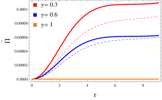
ฮ ยฏยฏฮ \displaystyle\bar{\Pi} =\displaystyle= r2โ€‹{3โˆ’2โ€‹ฯ‡6โ€‹(๐’ž12+3โ€‹r2)2}โ€‹(1โˆ’ฮณ)2โ€‹(ฯ‡3+4โ€‹ฯ€)โ€‹(๐’ž12+3โ€‹r2)2,superscript๐‘Ÿ232subscript๐œ’6superscriptsuperscriptsubscript๐’ž123superscript๐‘Ÿ221๐›พ2subscript๐œ’34๐œ‹superscriptsuperscriptsubscript๐’ž123superscript๐‘Ÿ22\displaystyle\frac{r^{2}\big{\{}3-2\chi_{6}\big{(}\mathcal{C}_{1}^{2}+3r^{2}\big{)}^{2}\big{\}}\big{(}1-\gamma\big{)}}{2\big{(}\chi_{3}+4\pi\big{)}\big{(}\mathcal{C}_{1}^{2}+3r^{2}\big{)}^{2}}, (46)

from which we clearly observe that this factor disappears when ฮณ=1๐›พ1\gamma=1, hence, the considered matter source becomes isotropic for this parametric value. Equations (43)-(46) provide the exact solution of fโ€‹(โ„,๐•‹)๐‘“โ„๐•‹f(\mathbb{R},\mathbb{T}) field equations where ฮณ๐›พ\gamma belongs to [0,1]01[0,1]. In this way, we can thoroughly follow the process of isotropizing the anisotropic fluid by taking variation in the decoupling parameter.

5 Complexity of Compact Sources

The notion of complexity was initially formulated for a static sphere [40] and then extended to the framework of dissipative dynamical matter configuration [41]. The basic idea to establish its definition is that there does not exist any factor that produces complexity in uniform/isotropic distribution. A specific factor that measures the complexity of a spacetime structure (i.e., ๐•Tโ€‹Fsubscript๐•๐‘‡๐น\mathbb{Y}_{TF}) is one of the four different scalars resulting from the orthogonal decomposition of the curvature tensor. By following Herreraโ€™s technique, we obtain this scalar factor possessing fโ€‹(โ„,๐•‹)๐‘“โ„๐•‹f(\mathbb{R},\mathbb{T}) corrections in the following form

๐•Tโ€‹Fโ€‹(r)=(1+ฯ‡3)โ€‹(8โ€‹ฯ€โ€‹ฮ +2โ€‹s2r4)โˆ’4โ€‹ฯ€r3โ€‹โˆซ0rr^3โ€‹ฮผโ€ฒโ€‹(r^)โ€‹๐‘‘r^.subscript๐•๐‘‡๐น๐‘Ÿ1subscript๐œ’38๐œ‹ฮ 2superscripts2superscript๐‘Ÿ44๐œ‹superscript๐‘Ÿ3superscriptsubscript0๐‘Ÿsuperscript^๐‘Ÿ3superscript๐œ‡โ€ฒ^๐‘Ÿdifferential-d^๐‘Ÿ\mathbb{Y}_{TF}(r)=\big{(}1+\chi_{3}\big{)}\bigg{(}8\pi\Pi+\frac{2\mathrm{s}^{2}}{r^{4}}\bigg{)}-\frac{4\pi}{r^{3}}\int_{0}^{r}\hat{r}^{3}\mu^{\prime}(\hat{r})d\hat{r}. (47)

The presence of an additional source in the current setup (12)-(14) makes the above complexity factor as

๐•ยฏTโ€‹Fโ€‹(r)subscriptยฏ๐•๐‘‡๐น๐‘Ÿ\displaystyle\bar{\mathbb{Y}}_{TF}(r) =\displaystyle= (1+ฯ‡3)โ€‹(8โ€‹ฯ€โ€‹ฮ ยฏ+2โ€‹s2r4)โˆ’4โ€‹ฯ€r3โ€‹โˆซ0rr^3โ€‹ฮผยฏโ€ฒโ€‹(r^)โ€‹๐‘‘r^1subscript๐œ’38๐œ‹ยฏฮ 2superscripts2superscript๐‘Ÿ44๐œ‹superscript๐‘Ÿ3superscriptsubscript0๐‘Ÿsuperscript^๐‘Ÿ3superscriptยฏ๐œ‡โ€ฒ^๐‘Ÿdifferential-d^๐‘Ÿ\displaystyle\big{(}1+\chi_{3}\big{)}\bigg{(}8\pi\bar{\Pi}+\frac{2\mathrm{s}^{2}}{r^{4}}\bigg{)}-\frac{4\pi}{r^{3}}\int_{0}^{r}\hat{r}^{3}\bar{\mu}^{\prime}(\hat{r})d\hat{r} (48)
=\displaystyle= (1+ฯ‡3)โ€‹(8โ€‹ฯ€โ€‹ฮ +2โ€‹s2r4)โˆ’4โ€‹ฯ€r3โ€‹โˆซ0rr^3โ€‹ฮผโ€ฒโ€‹(r^)โ€‹๐‘‘r^1subscript๐œ’38๐œ‹ฮ 2superscripts2superscript๐‘Ÿ44๐œ‹superscript๐‘Ÿ3superscriptsubscript0๐‘Ÿsuperscript^๐‘Ÿ3superscript๐œ‡โ€ฒ^๐‘Ÿdifferential-d^๐‘Ÿ\displaystyle\big{(}1+\chi_{3}\big{)}\bigg{(}8\pi\Pi+\frac{2\mathrm{s}^{2}}{r^{4}}\bigg{)}-\frac{4\pi}{r^{3}}\int_{0}^{r}\hat{r}^{3}\mu^{\prime}(\hat{r})d\hat{r}
+\displaystyle+ 8ฯ€ฮ โ„ญ(1+ฯ‡3)+4โ€‹ฯ€r3โˆซ0rr^3โ„ญโ€ฒ00(r^)dr^.\displaystyle 8\pi\Pi_{\mathfrak{C}}\big{(}1+\chi_{3}\big{)}+\frac{4\pi}{r^{3}}\int_{0}^{r}\hat{r}^{3}\mathfrak{C}{{}_{0}^{0}}^{\prime}(\hat{r})d\hat{r}.

We can analogously write the above equation as

๐•ยฏTโ€‹F=๐•Tโ€‹F+๐•Tโ€‹Fโ„ญ,subscriptยฏ๐•๐‘‡๐นsubscript๐•๐‘‡๐นsuperscriptsubscript๐•๐‘‡๐นโ„ญ\displaystyle\bar{\mathbb{Y}}_{TF}=\mathbb{Y}_{TF}+\mathbb{Y}_{TF}^{\mathfrak{C}}, (49)

where the sets (22)-(24) and (25)-(27) being represented by ๐•Tโ€‹Fsubscript๐•๐‘‡๐น\mathbb{Y}_{TF} and ๐•Tโ€‹Fโ„ญsuperscriptsubscript๐•๐‘‡๐นโ„ญ\mathbb{Y}_{TF}^{\mathfrak{C}}, respectively. Since the model (43)-(46) is established for the constraint ฮ ยฏ=0ยฏฮ 0\bar{\Pi}=0, Eq.(48) thus yields

๐•ยฏTโ€‹Fsubscriptยฏ๐•๐‘‡๐น\displaystyle\bar{\mathbb{Y}}_{TF} =\displaystyle= 2โ€‹s2r4โ€‹(1+ฯ‡3)โˆ’4โ€‹ฯ€r3โ€‹โˆซ0rr^3โ€‹ฮผยฏโ€ฒโ€‹(r^)โ€‹๐‘‘r^.2superscripts2superscript๐‘Ÿ41subscript๐œ’34๐œ‹superscript๐‘Ÿ3superscriptsubscript0๐‘Ÿsuperscript^๐‘Ÿ3superscriptยฏ๐œ‡โ€ฒ^๐‘Ÿdifferential-d^๐‘Ÿ\displaystyle\frac{2\mathrm{s}^{2}}{r^{4}}\big{(}1+\chi_{3}\big{)}-\frac{4\pi}{r^{3}}\int_{0}^{r}\hat{r}^{3}\bar{\mu}^{\prime}(\hat{r})d\hat{r}. (50)

Eq.(50) produces the following complexity factor after combining with the metric (42) and the modified field equations as

๐•ยฏTโ€‹Fsubscriptยฏ๐•๐‘‡๐น\displaystyle\bar{\mathbb{Y}}_{TF} =2โ€‹ฯ‡6โ€‹r2โ€‹(1+ฯ‡3)+130โ€‹r3โ€‹(ฯ‡3+2โ€‹ฯ€)โ€‹(ฯ‡3+4โ€‹ฯ€)โ€‹(๐’ž12+2โ€‹r2)2โ€‹(๐’ž12+3โ€‹r2)2absent2subscript๐œ’6superscript๐‘Ÿ21subscript๐œ’3130superscript๐‘Ÿ3subscript๐œ’32๐œ‹subscript๐œ’34๐œ‹superscriptsuperscriptsubscript๐’ž122superscript๐‘Ÿ22superscriptsuperscriptsubscript๐’ž123superscript๐‘Ÿ22\displaystyle=2\chi_{6}r^{2}\big{(}1+\chi_{3}\big{)}+\frac{1}{30r^{3}\big{(}\chi_{3}+2\pi\big{)}\big{(}\chi_{3}+4\pi\big{)}\big{(}\mathcal{C}_{1}^{2}+2r^{2}\big{)}^{2}\big{(}\mathcal{C}_{1}^{2}+3r^{2}\big{)}^{2}}
ร—[ฯ€๐’ž18r{5ฯ‡3(4r4(8ฯ‡6ฮณ+ฯ‡6)+3)+16ฯ€ฯ‡6(20ฮณ+3)r4}+5๐’ž16{48ฯ€2\displaystyle\times\bigg{[}\pi\mathcal{C}_{1}^{8}r\big{\{}5\chi_{3}\big{(}4r^{4}(8\chi_{6}\gamma+\chi_{6})+3\big{)}+16\pi\chi_{6}(20\gamma+3)r^{4}\big{\}}+5\mathcal{C}_{1}^{6}\big{\{}48\pi^{2}
ร—(2r7(6ฯ‡6ฮณ+ฯ‡6)โˆ’ฮณโ„‚1r5)โˆ’6ฮณโ„‚1r5ฯ‡32+ฯ€r3ฯ‡3(27โˆ’36ฮณโ„‚1r2+8ฯ‡6\displaystyle\times\big{(}2r^{7}(6\chi_{6}\gamma+\chi_{6})-\gamma\mathbb{C}_{1}r^{5}\big{)}-6\gamma\mathbb{C}_{1}r^{5}\chi_{3}^{2}+\pi r^{3}\chi_{3}\big{(}27-36\gamma\mathbb{C}_{1}r^{2}+8\chi_{6}
ร—(36ฮณ+5)r4)}+4๐’ž14r5{โˆ’45ฮณโ„‚1r2ฯ‡32+5ฯ€ฯ‡3(24(2โˆ’ฮณ)โˆ’54ฮณโ„‚1r2\displaystyle\times(36\gamma+5)r^{4}\big{)}\big{\}}+4\mathcal{C}_{1}^{4}r^{5}\big{\{}-45\gamma\mathbb{C}_{1}r^{2}\chi_{3}^{2}+5\pi\chi_{3}\big{(}24(2-\gamma)-54\gamma\mathbb{C}_{1}r^{2}
+ฯ‡6(240ฮณ+37)r4)+12ฯ€2(30โˆ’20ฮณโˆ’30ฮณโ„‚1r2+ฯ‡6(200ฮณ+37)r4)}\displaystyle+\chi_{6}(240\gamma+37)r^{4}\big{)}+12\pi^{2}\big{(}30-20\gamma-30\gamma\mathbb{C}_{1}r^{2}+\chi_{6}(200\gamma+37)r^{4}\big{)}\big{\}}
โˆ’53ฯ€๐’ž12ฯ‡3(๐’ž14+5๐’ž12r2+6r4)2tanโˆ’1(3โ€‹r๐’ž12)+30๐’ž12r7{2ฯ€ฯ‡3\displaystyle-5\sqrt{3}\pi\sqrt{\mathcal{C}_{1}^{2}}\chi_{3}\big{(}\mathcal{C}_{1}^{4}+5\mathcal{C}_{1}^{2}r^{2}+6r^{4}\big{)}^{2}\tan^{-1}\big{(}\frac{\sqrt{3}r}{\sqrt{\mathcal{C}_{1}^{2}}}\big{)}+30\mathcal{C}_{1}^{2}r^{7}\big{\{}2\pi\chi_{3}
ร—(45โˆ’24ฮณโˆ’27ฮณโ„‚1r2+20r4(6ฯ‡6ฮณ+ฯ‡6))โˆ’9ฮณโ„‚1r2ฯ‡32+24ฯ€2(8โˆ’4ฮณ\displaystyle\times\big{(}45-24\gamma-27\gamma\mathbb{C}_{1}r^{2}+20r^{4}(6\chi_{6}\gamma+\chi_{6})\big{)}-9\gamma\mathbb{C}_{1}r^{2}\chi_{3}^{2}+24\pi^{2}\big{(}8-4\gamma
โˆ’3ฮณโ„‚1r2+4r4(5ฯ‡6ฮณ+ฯ‡6))}+48ฯ€r9{5ฯ‡3(10โˆ’3ฮณ+3r4(6ฯ‡6ฮณ+ฯ‡6))\displaystyle-3\gamma\mathbb{C}_{1}r^{2}+4r^{4}(5\chi_{6}\gamma+\chi_{6})\big{)}\big{\}}+48\pi r^{9}\big{\{}5\chi_{3}\big{(}10-3\gamma+3r^{4}(6\chi_{6}\gamma+\chi_{6})\big{)}
+6ฯ€(6r4(5ฯ‡6ฮณ+ฯ‡6)โˆ’5(ฮณโˆ’4))}].\displaystyle+6\pi\big{(}6r^{4}(5\chi_{6}\gamma+\chi_{6})-5(\gamma-4)\big{)}\big{\}}\bigg{]}. (51)

5.1 Two Systems with the Same Complexity Factor

In this subsection, we consider that the scalar factor ๐•Tโ€‹Fsubscript๐•๐‘‡๐น\mathbb{Y}_{TF} representing the complexity of an initial matter source does not possess any change when a new gravitational source โ„ญฮฒโ€‹ฮฑsubscriptโ„ญ๐›ฝ๐›ผ\mathfrak{C}_{\beta\alpha} is added, i.e., ๐•Tโ€‹Fโ„ญ=0superscriptsubscript๐•๐‘‡๐นโ„ญ0\mathbb{Y}_{TF}^{\mathfrak{C}}=0. This constraint results in ๐•ยฏTโ€‹F=๐•Tโ€‹Fsubscriptยฏ๐•๐‘‡๐นsubscript๐•๐‘‡๐น\bar{\mathbb{Y}}_{TF}=\mathbb{Y}_{TF} or

8ฯ€ฮ โ„ญ(1+ฯ‡3)=โˆ’4โ€‹ฯ€r3โˆซ0rr^3โ„ญโ€ฒ00(r^)dr^.\displaystyle 8\pi\Pi_{\mathfrak{C}}\big{(}1+\chi_{3}\big{)}=-\frac{4\pi}{r^{3}}\int_{0}^{r}\hat{r}^{3}\mathfrak{C}{{}_{0}^{0}}^{\prime}(\hat{r})d\hat{r}. (52)

We use Eq.(25) to manipulate the right side of (52) as

โˆ’4โ€‹ฯ€r3โˆซ0rr^3โ„ญโ€ฒ00(r^)dr^=โˆ’12โ€‹r(โ„ฑโ€ฒโˆ’2โ€‹โ„ฑr),\displaystyle-\frac{4\pi}{r^{3}}\int_{0}^{r}\hat{r}^{3}\mathfrak{C}{{}_{0}^{0}}^{\prime}(\hat{r})d\hat{r}=-\frac{1}{2r}\bigg{(}\mathcal{F}^{\prime}-\frac{2\mathcal{F}}{r}\bigg{)}, (53)

yielding the condition (52) as the following first-order differential equation given by

(ฯ‡3+1)โ€‹{โ„ฑโ€ฒโ€‹(r)โ€‹(ฯ‡1โ€ฒ4+12โ€‹r)+โ„ฑโ€‹(r)โ€‹(ฯ‡1โ€ฒโ€ฒ2โˆ’1r2+ฯ‡1โ€ฒโฃ24โˆ’ฯ‡1โ€ฒ2โ€‹r)}subscript๐œ’31superscriptโ„ฑโ€ฒ๐‘Ÿsuperscriptsubscript๐œ’1โ€ฒ412๐‘Ÿโ„ฑ๐‘Ÿsuperscriptsubscript๐œ’1โ€ฒโ€ฒ21superscript๐‘Ÿ2superscriptsubscript๐œ’1โ€ฒ24superscriptsubscript๐œ’1โ€ฒ2๐‘Ÿ\displaystyle(\chi_{3}+1)\bigg{\{}\mathcal{F}^{\prime}(r)\bigg{(}\frac{\chi_{1}^{\prime}}{4}+\frac{1}{2r}\bigg{)}+\mathcal{F}(r)\bigg{(}\frac{\chi_{1}^{\prime\prime}}{2}-\frac{1}{r^{2}}+\frac{\chi_{1}^{\prime 2}}{4}-\frac{\chi_{1}^{\prime}}{2r}\bigg{)}\bigg{\}}
+12โ€‹rโ€‹(โ„ฑโ€ฒโˆ’2โ€‹โ„ฑr)=0.12๐‘Ÿsuperscriptโ„ฑโ€ฒ2โ„ฑ๐‘Ÿ0\displaystyle+\frac{1}{2r}\bigg{(}\mathcal{F}^{\prime}-\frac{2\mathcal{F}}{r}\bigg{)}=0. (54)

This equation possesses the temporal metric function describing the original anisotropic matter field, hence increases the unknowns. The Tolman IV ansatz is used in this regard to make the system solvable as

ฯ‡1โ€‹(r)subscript๐œ’1๐‘Ÿ\displaystyle\chi_{1}(r) =lnโก{๐’ž22โ€‹(1+r2๐’ž12)},absentsuperscriptsubscript๐’ž221superscript๐‘Ÿ2superscriptsubscript๐’ž12\displaystyle=\ln\bigg{\{}\mathcal{C}_{2}^{2}\bigg{(}1+\frac{r^{2}}{\mathcal{C}_{1}^{2}}\bigg{)}\bigg{\}}, (55)
ฯ‡5โ€‹(r)subscript๐œ’5๐‘Ÿ\displaystyle\chi_{5}(r) =eโˆ’ฯ‡2=(๐’ž12+r2)โ€‹(๐’ž32โˆ’r2)๐’ž32โ€‹(๐’ž12+2โ€‹r2),absentsuperscript๐‘’subscript๐œ’2superscriptsubscript๐’ž12superscript๐‘Ÿ2superscriptsubscript๐’ž32superscript๐‘Ÿ2superscriptsubscript๐’ž32superscriptsubscript๐’ž122superscript๐‘Ÿ2\displaystyle=e^{-\chi_{2}}=\frac{\big{(}\mathcal{C}_{1}^{2}+r^{2}\big{)}\big{(}\mathcal{C}_{3}^{2}-r^{2}\big{)}}{\mathcal{C}_{3}^{2}\big{(}\mathcal{C}_{1}^{2}+2r^{2}\big{)}}, (56)

triggered by the density and pressure isotropy as

ฮผ๐œ‡\displaystyle\mu =112โ€‹๐’ž32โ€‹(ฯ‡3+2โ€‹ฯ€)โ€‹(ฯ‡3+4โ€‹ฯ€)โ€‹(๐’ž12+2โ€‹r2)2absent112superscriptsubscript๐’ž32subscript๐œ’32๐œ‹subscript๐œ’34๐œ‹superscriptsuperscriptsubscript๐’ž122superscript๐‘Ÿ22\displaystyle=\frac{1}{12\mathcal{C}_{3}^{2}\big{(}\chi_{3}+2\pi\big{)}\big{(}\chi_{3}+4\pi\big{)}\big{(}\mathcal{C}_{1}^{2}+2r^{2}\big{)}^{2}}
ร—[๐’ž14{12(ฯ‡3+3ฯ€)โˆ’ฯ‡6๐’ž32r2(5ฯ‡3+12ฯ€)}+๐’ž12{12r2(2ฯ‡3+7ฯ€)โˆ’๐’ž32\displaystyle\times\big{[}\mathcal{C}_{1}^{4}\big{\{}12(\chi_{3}+3\pi)-\chi_{6}\mathcal{C}_{3}^{2}r^{2}(5\chi_{3}+12\pi)\big{\}}+\mathcal{C}_{1}^{2}\big{\{}12r^{2}(2\chi_{3}+7\pi)-\mathcal{C}_{3}^{2}
ร—(5ฯ‡3+12ฯ€)(4ฯ‡6r4โˆ’3)}+2r2{9r2(ฯ‡3+4ฯ€)โˆ’2๐’ž32(5ฯ‡6r4ฯ‡3โˆ’3ฯ‡3\displaystyle\times(5\chi_{3}+12\pi)\big{(}4\chi_{6}r^{4}-3\big{)}\big{\}}+2r^{2}\big{\{}9r^{2}(\chi_{3}+4\pi)-2\mathcal{C}_{3}^{2}\big{(}5\chi_{6}r^{4}\chi_{3}-3\chi_{3}
+12ฯ€ฯ‡6r4โˆ’6ฯ€)}],\displaystyle+12\pi\chi_{6}r^{4}-6\pi\big{)}\big{\}}\big{]}, (57)
P๐‘ƒ\displaystyle P =112โ€‹๐’ž32โ€‹(ฯ‡3+2โ€‹ฯ€)โ€‹(ฯ‡3+4โ€‹ฯ€)โ€‹(๐’ž12+2โ€‹r2)2absent112superscriptsubscript๐’ž32subscript๐œ’32๐œ‹subscript๐œ’34๐œ‹superscriptsuperscriptsubscript๐’ž122superscript๐‘Ÿ22\displaystyle=\frac{1}{12\mathcal{C}_{3}^{2}\big{(}\chi_{3}+2\pi\big{)}\big{(}\chi_{3}+4\pi\big{)}\big{(}\mathcal{C}_{1}^{2}+2r^{2}\big{)}^{2}}
ร—[๐’ž14{ฯ‡6๐’ž32r2(5ฯ‡3+12ฯ€)โˆ’12ฯ€}+๐’ž12{๐’ž32(20ฯ‡6r4ฯ‡3+48ฯ€ฯ‡6r4+12ฯ€\displaystyle\times\big{[}\mathcal{C}_{1}^{4}\big{\{}\chi_{6}\mathcal{C}_{3}^{2}r^{2}(5\chi_{3}+12\pi)-12\pi\big{\}}+\mathcal{C}_{1}^{2}\big{\{}\mathcal{C}_{3}^{2}\big{(}20\chi_{6}r^{4}\chi_{3}+48\pi\chi_{6}r^{4}+12\pi
+9ฯ‡3)โˆ’12r2(ฯ‡3+5ฯ€)}+2r2(2๐’ž32{5ฯ‡6r4ฯ‡3+12ฯ€ฯ‡6r4+3ฯ‡3+6ฯ€}\displaystyle+9\chi_{3}\big{)}-12r^{2}(\chi_{3}+5\pi)\big{\}}+2r^{2}\big{(}2\mathcal{C}_{3}^{2}\big{\{}5\chi_{6}r^{4}\chi_{3}+12\pi\chi_{6}r^{4}+3\chi_{3}+6\pi\big{\}}
โˆ’9r2(ฯ‡3+4ฯ€))].\displaystyle-9r^{2}(\chi_{3}+4\pi)\big{)}\big{]}. (58)

Equations (37) and (38) supply the unknowns ๐’ž12superscriptsubscript๐’ž12\mathcal{C}_{1}^{2} and ๐’ž22superscriptsubscript๐’ž22\mathcal{C}_{2}^{2}, whereas ๐’ž32superscriptsubscript๐’ž32\mathcal{C}_{3}^{2} has the following form

๐’ž32superscriptsubscript๐’ž32\displaystyle\mathcal{C}_{3}^{2} =2โ€‹โ„›3โ€‹(๐’ฎยฏ2โˆ’2โ€‹โ„ณยฏโ€‹โ„›+โ„›2)2โ€‹โ„ณยฏโ€‹๐’ฎยฏโˆ’4โ€‹โ„ณยฏ2โ€‹โ„›+๐’ฎยฏโ€‹โ„›+2โ€‹โ„ณยฏโ€‹โ„›2.absent2superscriptโ„›3superscriptยฏ๐’ฎ22ยฏโ„ณโ„›superscriptโ„›22ยฏโ„ณยฏ๐’ฎ4superscriptยฏโ„ณ2โ„›ยฏ๐’ฎโ„›2ยฏโ„ณsuperscriptโ„›2\displaystyle=\frac{2\mathcal{R}^{3}\big{(}\bar{\mathcal{S}}^{2}-2\bar{\mathcal{M}}\mathcal{R}+\mathcal{R}^{2}\big{)}}{2\bar{\mathcal{M}}\bar{\mathcal{S}}-4\bar{\mathcal{M}}^{2}\mathcal{R}+\bar{\mathcal{S}}\mathcal{R}+2\bar{\mathcal{M}}\mathcal{R}^{2}}. (59)

Insertion of gtโ€‹tsubscript๐‘”๐‘ก๐‘กg_{tt} metric component (55) in Eq.(54) gives

โ„ฑโ€‹(r)=โ„‚2โ€‹r2โ€‹(๐’ž12+r2)๐’ž12โ€‹(2+ฯ‡3)+r2โ€‹(2โ€‹ฯ‡3+3),โ„ฑ๐‘Ÿsubscriptโ„‚2superscript๐‘Ÿ2superscriptsubscript๐’ž12superscript๐‘Ÿ2superscriptsubscript๐’ž122subscript๐œ’3superscript๐‘Ÿ22subscript๐œ’33\mathcal{F}(r)=\frac{\mathbb{C}_{2}r^{2}\big{(}\mathcal{C}_{1}^{2}+r^{2}\big{)}}{\mathcal{C}_{1}^{2}\big{(}2+\chi_{3}\big{)}+r^{2}\big{(}2\chi_{3}+3\big{)}}, (60)

involving โ„‚2subscriptโ„‚2\mathbb{C}_{2} as a constant of integration. Consequently, the deformed expression of grโ€‹rsubscript๐‘”๐‘Ÿ๐‘Ÿg_{rr} component becomes

eฯ‡2superscript๐‘’subscript๐œ’2\displaystyle e^{\chi_{2}} =ฯ‡5โˆ’1=๐’ž32โ€‹(๐’ž12+2โ€‹r2)(๐’ž12+r2)โ€‹{๐’ž32+r2โ€‹(ฮณโ€‹โ„‚2โ€‹๐’ž32โ€‹(๐’ž12+2โ€‹r2)๐’ž12โ€‹(2+ฯ‡3)+r2โ€‹(2โ€‹ฯ‡3+3)โˆ’1)}โˆ’1,absentsuperscriptsubscript๐œ’51superscriptsubscript๐’ž32superscriptsubscript๐’ž122superscript๐‘Ÿ2superscriptsubscript๐’ž12superscript๐‘Ÿ2superscriptsuperscriptsubscript๐’ž32superscript๐‘Ÿ2๐›พsubscriptโ„‚2superscriptsubscript๐’ž32superscriptsubscript๐’ž122superscript๐‘Ÿ2superscriptsubscript๐’ž122subscript๐œ’3superscript๐‘Ÿ22subscript๐œ’3311\displaystyle=\chi_{5}^{-1}=\frac{\mathcal{C}_{3}^{2}\big{(}\mathcal{C}_{1}^{2}+2r^{2}\big{)}}{\big{(}\mathcal{C}_{1}^{2}+r^{2}\big{)}}\bigg{\{}\mathcal{C}_{3}^{2}+r^{2}\bigg{(}\frac{\gamma\mathbb{C}_{2}\mathcal{C}_{3}^{2}\big{(}\mathcal{C}_{1}^{2}+2r^{2}\big{)}}{\mathcal{C}_{1}^{2}\big{(}2+\chi_{3}\big{)}+r^{2}\big{(}2\chi_{3}+3\big{)}}-1\bigg{)}\bigg{\}}^{-1}, (61)

and the total complexity factor ๐•ยฏTโ€‹Fsubscriptยฏ๐•๐‘‡๐น\bar{\mathbb{Y}}_{TF} defined in Eq.(48) leads to

๐•ยฏTโ€‹Fsubscriptยฏ๐•๐‘‡๐น\displaystyle\bar{\mathbb{Y}}_{TF} =๐•Tโ€‹F=116โ€‹r3โ€‹๐’ž32โ€‹(ฯ‡3+2โ€‹ฯ€)โ€‹(ฯ‡3+4โ€‹ฯ€)โ€‹(๐’ž12+2โ€‹r2)2[2r{45ฯ€๐’ž16ฯ‡3\displaystyle=\mathbb{Y}_{TF}=\frac{1}{16r^{3}\mathcal{C}_{3}^{2}\big{(}\chi_{3}+2\pi\big{)}\big{(}\chi_{3}+4\pi\big{)}\big{(}\mathcal{C}_{1}^{2}+2r^{2}\big{)}^{2}}\bigg{[}2r\big{\{}45\pi\mathcal{C}_{1}^{6}\chi_{3}
+2๐’ž14(120ฯ‡6r4๐’ž32ฯ‡32(ฯ‡3+1)+96ฯ€2ฯ‡6r4๐’ž32+5ฯ€ฯ‡3(8(6ฯ‡3+7)\displaystyle+2\mathcal{C}_{1}^{4}\big{(}120\chi_{6}r^{4}\mathcal{C}_{3}^{2}\chi_{3}^{2}(\chi_{3}+1)+96\pi^{2}\chi_{6}r^{4}\mathcal{C}_{3}^{2}+5\pi\chi_{3}\big{(}8(6\chi_{3}+7)
ร—ฯ‡6r4๐’ž32+15r2+9๐’ž32))+4๐’ž12(240ฯ‡6r6๐’ž32ฯ‡32(ฯ‡3+1)+5ฯ€r2ฯ‡3\displaystyle\times\chi_{6}r^{4}\mathcal{C}_{3}^{2}+15r^{2}+9\mathcal{C}_{3}^{2}\big{)}\big{)}+4\mathcal{C}_{1}^{2}\big{(}240\chi_{6}r^{6}\mathcal{C}_{3}^{2}\chi_{3}^{2}(\chi_{3}+1)+5\pi r^{2}\chi_{3}
ร—(16ฯ‡6r4๐’ž32(6ฯ‡3+7)+24r2+15๐’ž32)+48ฯ€2r4(4ฯ‡6r2๐’ž32+5))\displaystyle\times\big{(}16\chi_{6}r^{4}\mathcal{C}_{3}^{2}(6\chi_{3}+7)+24r^{2}+15\mathcal{C}_{3}^{2}\big{)}+48\pi^{2}r^{4}\big{(}4\chi_{6}r^{2}\mathcal{C}_{3}^{2}+5\big{)}\big{)}
+64r4๐’ž32(15ฯ‡6r4ฯ‡32(ฯ‡3+1)+5ฯ€ฯ‡3(ฯ‡6r4(6ฯ‡3+7)+3)+6ฯ€2\displaystyle+64r^{4}\mathcal{C}_{3}^{2}\big{(}15\chi_{6}r^{4}\chi_{3}^{2}(\chi_{3}+1)+5\pi\chi_{3}\big{(}\chi_{6}r^{4}(6\chi_{3}+7)+3\big{)}+6\pi^{2}
ร—(2ฯ‡6r4+5))}โˆ’452ฯ€๐’ž12ฯ‡3(๐’ž12+2r2)2(๐’ž12+2๐’ž32)tanโˆ’1(2โ€‹r๐’ž12)].\displaystyle\times\big{(}2\chi_{6}r^{4}+5\big{)}\big{)}\big{\}}-45\sqrt{2}\pi\sqrt{\mathcal{C}_{1}^{2}}\chi_{3}\big{(}\mathcal{C}_{1}^{2}+2r^{2}\big{)}^{2}(\mathcal{C}_{1}^{2}+2\mathcal{C}_{3}^{2})\tan^{-1}\bigg{(}\frac{\sqrt{2}r}{\sqrt{\mathcal{C}_{1}^{2}}}\bigg{)}\bigg{]}. (62)

5.2 Constructing Solutions with Null Complexity

This subsection establishes a solution to the fโ€‹(โ„,๐•‹)๐‘“โ„๐•‹f(\mathbb{R},\mathbb{T}) field equations for a particular constraint depending on the complexity factor. It is considered that the original anisotropic source does possess the complexity such that ๐•Tโ€‹Fโ‰ 0subscript๐•๐‘‡๐น0\mathbb{Y}_{TF}\neq 0, however, the system becomes free from complexity once a new gravitational source is added. This can mathematically be expressed by ๐•ยฏTโ€‹F=0subscriptยฏ๐•๐‘‡๐น0\bar{\mathbb{Y}}_{TF}=0, that leads Eq.(49) in terms of ansatz (55) and (56) to

120โ€‹rโ€‹(ฯ‡6+1)(๐’ž12+r2)2โ€‹[rโ€‹(๐’ž14+3โ€‹๐’ž12โ€‹r2+2โ€‹r4)โ€‹โ„ฑโ€ฒโ€‹(r)โˆ’2โ€‹(๐’ž14+2โ€‹๐’ž12โ€‹r2+2โ€‹r4)โ€‹โ„ฑโ€‹(r)]120๐‘Ÿsubscript๐œ’61superscriptsuperscriptsubscript๐’ž12superscript๐‘Ÿ22delimited-[]๐‘Ÿsuperscriptsubscript๐’ž143superscriptsubscript๐’ž12superscript๐‘Ÿ22superscript๐‘Ÿ4superscriptโ„ฑโ€ฒ๐‘Ÿ2superscriptsubscript๐’ž142superscriptsubscript๐’ž12superscript๐‘Ÿ22superscript๐‘Ÿ4โ„ฑ๐‘Ÿ\displaystyle\frac{120r\big{(}\chi_{6}+1\big{)}}{\big{(}\mathcal{C}_{1}^{2}+r^{2}\big{)}^{2}}\big{[}r\big{(}\mathcal{C}_{1}^{4}+3\mathcal{C}_{1}^{2}r^{2}+2r^{4}\big{)}\mathcal{F}^{\prime}(r)-2\big{(}\mathcal{C}_{1}^{4}+2\mathcal{C}_{1}^{2}r^{2}+2r^{4}\big{)}\mathcal{F}(r)\big{]}
+1(ฯ‡3+2โ€‹ฯ€)โ€‹(ฯ‡3+4โ€‹ฯ€)โ€‹๐’ž32โ€‹(๐’ž12+2โ€‹r2)2[2r(45ฯ€๐’ž16ฯ‡3+2๐’ž14(120ฯ‡6r4๐’ž32ฯ‡32\displaystyle+\frac{1}{\big{(}\chi_{3}+2\pi\big{)}\big{(}\chi_{3}+4\pi\big{)}\mathcal{C}_{3}^{2}\big{(}\mathcal{C}_{1}^{2}+2r^{2}\big{)}^{2}}\bigg{[}2r\big{(}45\pi\mathcal{C}_{1}^{6}\chi_{3}+2\mathcal{C}_{1}^{4}\big{(}120\chi_{6}r^{4}\mathcal{C}_{3}^{2}\chi_{3}^{2}
ร—(ฯ‡3+1)+96ฯ€2ฯ‡6r4๐’ž32+5ฯ€ฯ‡3(8ฯ‡6r4๐’ž32(6ฯ‡3+7)+15r2+9๐’ž32))\displaystyle\times(\chi_{3}+1)+96\pi^{2}\chi_{6}r^{4}\mathcal{C}_{3}^{2}+5\pi\chi_{3}\big{(}8\chi_{6}r^{4}\mathcal{C}_{3}^{2}(6\chi_{3}+7)+15r^{2}+9\mathcal{C}_{3}^{2}\big{)}\big{)}
+4๐’ž12(240ฯ‡6r6๐’ž32ฯ‡32(ฯ‡3+1)+5ฯ€r2ฯ‡3(24r2+15๐’ž32+16(6ฯ‡3+7)\displaystyle+4\mathcal{C}_{1}^{2}\big{(}240\chi_{6}r^{6}\mathcal{C}_{3}^{2}\chi_{3}^{2}(\chi_{3}+1)+5\pi r^{2}\chi_{3}\big{(}24r^{2}+15\mathcal{C}_{3}^{2}+16(6\chi_{3}+7)
ร—ฯ‡6r4๐’ž32)+48ฯ€2r4(4ฯ‡6r2๐’ž32+5))+64r4๐’ž32(15ฯ‡6r4ฯ‡32(ฯ‡3+1)+5ฯ€ฯ‡3\displaystyle\times\chi_{6}r^{4}\mathcal{C}_{3}^{2}\big{)}+48\pi^{2}r^{4}\big{(}4\chi_{6}r^{2}\mathcal{C}_{3}^{2}+5\big{)}\big{)}+64r^{4}\mathcal{C}_{3}^{2}\big{(}15\chi_{6}r^{4}\chi_{3}^{2}(\chi_{3}+1)+5\pi\chi_{3}
ร—(ฯ‡6r4(6ฯ‡3+7)+3)+6ฯ€2(2ฯ‡6r4+5)))โˆ’452ฯ€๐’ž12ฯ‡3(๐’ž12+2r2)2\displaystyle\times\big{(}\chi_{6}r^{4}(6\chi_{3}+7)+3\big{)}+6\pi^{2}\big{(}2\chi_{6}r^{4}+5\big{)}\big{)}\big{)}-45\sqrt{2}\pi\sqrt{\mathcal{C}_{1}^{2}}\chi_{3}\big{(}\mathcal{C}_{1}^{2}+2r^{2}\big{)}^{2}
ร—(๐’ž12+2๐’ž32)tanโˆ’1(2โ€‹r๐’ž12)]โˆ’120r(2โ„ฑ(r)โˆ’rโ„ฑโ€ฒ(r))=0.\displaystyle\times(\mathcal{C}_{1}^{2}+2\mathcal{C}_{3}^{2})\tan^{-1}\bigg{(}\frac{\sqrt{2}r}{\sqrt{\mathcal{C}_{1}^{2}}}\bigg{)}\bigg{]}-120r\big{(}2\mathcal{F}(r)-r\mathcal{F}^{\prime}(r)\big{)}=0. (63)

The solution belonging to the above equation is

โ„ฑโ€‹(r)โ„ฑ๐‘Ÿ\displaystyle\mathcal{F}(r) =r2โ€‹(๐’ž12+r2)120โ€‹๐’ž32โ€‹(ฯ‡32+6โ€‹ฯ€โ€‹ฯ‡3+8โ€‹ฯ€2)โ€‹(ฯ‡3โ€‹๐’ž12+2โ€‹๐’ž12+2โ€‹ฯ‡3โ€‹r2+3โ€‹r2)[(๐’ž12+2๐’ž32)\displaystyle=\frac{r^{2}\big{(}\mathcal{C}_{1}^{2}+r^{2}\big{)}}{120\mathcal{C}_{3}^{2}\big{(}\chi_{3}^{2}+6\pi\chi_{3}+8\pi^{2}\big{)}\big{(}\chi_{3}\mathcal{C}_{1}^{2}+2\mathcal{C}_{1}^{2}+2\chi_{3}r^{2}+3r^{2}\big{)}}\bigg{[}\big{(}\mathcal{C}_{1}^{2}+2\mathcal{C}_{3}^{2}\big{)}
ร—{30โ€‹ฯ€โ€‹ฯ‡3r2+60โ€‹ฯ€โ€‹(3โ€‹ฯ‡3+8โ€‹ฯ€)๐’ž12+2โ€‹r2โˆ’15โ€‹ฯ‡3โ€‹2โ€‹๐’ž12โ€‹tanโˆ’1โก(2โ€‹rC12)r3}โˆ’16โ€‹ฯ‡6โ€‹r2absent30๐œ‹subscript๐œ’3superscript๐‘Ÿ260๐œ‹3subscript๐œ’38๐œ‹superscriptsubscript๐’ž122superscript๐‘Ÿ215subscript๐œ’32superscriptsubscript๐’ž12superscript12๐‘Ÿsuperscriptsubscript๐ถ12superscript๐‘Ÿ316subscript๐œ’6superscript๐‘Ÿ2\displaystyle\times\bigg{\{}\frac{30\pi\chi_{3}}{r^{2}}+\frac{60\pi(3\chi_{3}+8\pi)}{\mathcal{C}_{1}^{2}+2r^{2}}-\frac{15\chi_{3}\sqrt{2\mathcal{C}_{1}^{2}}\tan^{-1}\bigg{(}\frac{\sqrt{2}r}{\sqrt{C}_{1}^{2}}\bigg{)}}{r^{3}}\bigg{\}}-16\chi_{6}r^{2}
ร—{12ฯ€2+15ฯ‡32(1+ฯ‡3)+5ฯ€ฯ‡3(7+6ฯ‡3)}]+โ„‚3โ€‹r2โ€‹(๐’ž12+r2)ฯ‡3โ€‹๐’ž12+2โ€‹๐’ž12+2โ€‹ฯ‡3โ€‹r2+3โ€‹r2,\displaystyle\times\big{\{}12\pi^{2}+15\chi_{3}^{2}(1+\chi_{3})+5\pi\chi_{3}(7+6\chi_{3})\big{\}}\bigg{]}+\frac{\mathbb{C}_{3}r^{2}\big{(}\mathcal{C}_{1}^{2}+r^{2}\big{)}}{\chi_{3}\mathcal{C}_{1}^{2}+2\mathcal{C}_{1}^{2}+2\chi_{3}r^{2}+3r^{2}}, (64)

where โ„‚3subscriptโ„‚3\mathbb{C}_{3} being an integration constant with dimension 1โ„“21superscriptโ„“2\frac{1}{\ell^{2}}. The transformation (18) modifies the radial coefficient in terms of the function (64) as

eฯ‡2superscript๐‘’subscript๐œ’2\displaystyle e^{\chi_{2}} =ฯ‡5โˆ’1=๐’ž32โ€‹(๐’ž12+2โ€‹r2)(๐’ž12+r2)โ€‹(๐’ž32โˆ’r2)+ฮณโ€‹๐’ž32โ€‹โ„ฑโ€‹(r)โ€‹(๐’ž12+2โ€‹r2).absentsuperscriptsubscript๐œ’51superscriptsubscript๐’ž32superscriptsubscript๐’ž122superscript๐‘Ÿ2superscriptsubscript๐’ž12superscript๐‘Ÿ2superscriptsubscript๐’ž32superscript๐‘Ÿ2๐›พsuperscriptsubscript๐’ž32โ„ฑ๐‘Ÿsuperscriptsubscript๐’ž122superscript๐‘Ÿ2\displaystyle=\chi_{5}^{-1}=\frac{\mathcal{C}_{3}^{2}\big{(}\mathcal{C}_{1}^{2}+2r^{2}\big{)}}{\big{(}\mathcal{C}_{1}^{2}+r^{2}\big{)}\big{(}\mathcal{C}_{3}^{2}-r^{2}\big{)}+\gamma\mathcal{C}_{3}^{2}\mathcal{F}(r)\big{(}\mathcal{C}_{1}^{2}+2r^{2}\big{)}}. (65)

Hence, the corresponding matter determinants take the final form as

ฮผยฏยฏ๐œ‡\displaystyle\bar{\mu} =9โ€‹๐’ž12โ€‹(3โ€‹ฯ‡3+8โ€‹ฯ€)โˆ’r2โ€‹(5โ€‹ฯ‡3+12โ€‹ฯ€)โ€‹ฯ‡6โ€‹(๐’ž12+3โ€‹r2)2+6โ€‹r2โ€‹(5โ€‹ฯ‡3+12โ€‹ฯ€)12โ€‹(ฯ‡3+2โ€‹ฯ€)โ€‹(ฯ‡3+4โ€‹ฯ€)โ€‹(๐’ž12+3โ€‹r2)2absent9superscriptsubscript๐’ž123subscript๐œ’38๐œ‹superscript๐‘Ÿ25subscript๐œ’312๐œ‹subscript๐œ’6superscriptsuperscriptsubscript๐’ž123superscript๐‘Ÿ226superscript๐‘Ÿ25subscript๐œ’312๐œ‹12subscript๐œ’32๐œ‹subscript๐œ’34๐œ‹superscriptsuperscriptsubscript๐’ž123superscript๐‘Ÿ22\displaystyle=\frac{9\mathcal{C}_{1}^{2}\big{(}3\chi_{3}+8\pi\big{)}-r^{2}\big{(}5\chi_{3}+12\pi\big{)}\chi_{6}\big{(}\mathcal{C}_{1}^{2}+3r^{2}\big{)}^{2}+6r^{2}\big{(}5\chi_{3}+12\pi\big{)}}{12\big{(}\chi_{3}+2\pi\big{)}\big{(}\chi_{3}+4\pi\big{)}\big{(}\mathcal{C}_{1}^{2}+3r^{2}\big{)}^{2}}
โˆ’ฮณ960โ€‹ฯ€โ€‹๐’ž32โ€‹(๐’ž12โ€‹(ฯ‡3+2)+r2โ€‹(2โ€‹ฯ‡3+3))2[120๐’ž32โ„‚3(๐’ž12r2(7ฯ‡3+13)+3\displaystyle-\frac{\gamma}{960\pi\mathcal{C}_{3}^{2}\big{(}\mathcal{C}_{1}^{2}\big{(}\chi_{3}+2\big{)}+r^{2}\big{(}2\chi_{3}+3\big{)}\big{)}^{2}}\bigg{[}120\mathcal{C}_{3}^{2}\mathbb{C}_{3}\big{(}\mathcal{C}_{1}^{2}r^{2}\big{(}7\chi_{3}+13\big{)}+3
ร—๐’ž14(ฯ‡3+2)+3r4(2ฯ‡3+3))+30โ€‹ฯ€โ€‹๐’ž12rโ€‹(ฯ‡3+2โ€‹ฯ€)โ€‹(ฯ‡3+4โ€‹ฯ€)โ€‹(๐’ž12+2โ€‹r2)2\displaystyle\times\mathcal{C}_{1}^{4}\big{(}\chi_{3}+2\big{)}+3r^{4}\big{(}2\chi_{3}+3\big{)}\big{)}+\frac{30\pi\mathcal{C}_{1}^{2}}{r\big{(}\chi_{3}+2\pi\big{)}\big{(}\chi_{3}+4\pi\big{)}\big{(}\mathcal{C}_{1}^{2}+2r^{2}\big{)}^{2}}
ร—{4๐’ž12r5(ฯ‡3(14ฯ‡3+32ฯ€+27)+60ฯ€)+8๐’ž14r3(ฯ‡3(7ฯ‡3+18ฯ€+14)\displaystyle\times\bigg{\{}4\mathcal{C}_{1}^{2}r^{5}\big{(}\chi_{3}\big{(}14\chi_{3}+32\pi+27\big{)}+60\pi\big{)}+8\mathcal{C}_{1}^{4}r^{3}\big{(}\chi_{3}\big{(}7\chi_{3}+18\pi+14\big{)}
+34ฯ€)+42๐’ž13r4ฯ‡3(ฯ‡3+1)tanโˆ’1(2โ€‹rC12)+42๐’ž15r2ฯ‡3(ฯ‡3+1)\displaystyle+34\pi\big{)}+4\sqrt{2}\mathcal{C}_{1}^{3}r^{4}\chi_{3}\big{(}\chi_{3}+1\big{)}\tan^{-1}\bigg{(}\frac{\sqrt{2}r}{\sqrt{C_{1}^{2}}}\bigg{)}+4\sqrt{2}\mathcal{C}_{1}^{5}r^{2}\chi_{3}\big{(}\chi_{3}+1\big{)}
ร—tanโˆ’1โก(2โ€‹r๐’ž12)+2โ€‹๐’ž16โ€‹rโ€‹(ฯ‡3โ€‹(9โ€‹ฯ‡3+24โ€‹ฯ€+19)+48โ€‹ฯ€)+2โ€‹(ฯ‡3+1)absentsuperscript12๐‘Ÿsuperscriptsubscript๐’ž122superscriptsubscript๐’ž16๐‘Ÿsubscript๐œ’39subscript๐œ’324๐œ‹1948๐œ‹2subscript๐œ’31\displaystyle\times\tan^{-1}\bigg{(}\frac{\sqrt{2}r}{\sqrt{\mathcal{C}_{1}^{2}}}\bigg{)}+2\mathcal{C}_{1}^{6}r\big{(}\chi_{3}\big{(}9\chi_{3}+24\pi+19\big{)}+48\pi\big{)}+\sqrt{2}\big{(}\chi_{3}+1\big{)}
ร—๐’ž17ฯ‡3tanโˆ’1(2โ€‹r๐’ž12)+16r7(ฯ‡3+2ฯ€)(2ฯ‡3+3)}+4๐’ž32{r(ฯ‡3+2ฯ€)\displaystyle\times\mathcal{C}_{1}^{7}\chi_{3}\tan^{-1}\bigg{(}\frac{\sqrt{2}r}{\sqrt{\mathcal{C}_{1}^{2}}}\bigg{)}+16r^{7}\big{(}\chi_{3}+2\pi\big{)}\big{(}2\chi_{3}+3\big{)}\bigg{\}}+4\mathcal{C}_{3}^{2}\big{\{}r\big{(}\chi_{3}+2\pi\big{)}
ร—(ฯ‡3+4ฯ€)(๐’ž12+2r2)2}โˆ’1{6๐’ž16r(5ฯ€(ฯ‡3(9ฯ‡3+24ฯ€+19)+48ฯ€)\displaystyle\times\big{(}\chi_{3}+4\pi\big{)}\big{(}\mathcal{C}_{1}^{2}+2r^{2}\big{)}^{2}\big{\}}^{-1}\bigg{\{}6\mathcal{C}_{1}^{6}r\big{(}5\pi\big{(}\chi_{3}\big{(}9\chi_{3}+24\pi+19\big{)}+48\pi\big{)}
โˆ’2r4(11ฯ‡3+21)(5ฯ‡3(3ฯ‡3(ฯ‡3+2ฯ€+1)+7ฯ€)+12ฯ€2)ฯ‡6)+602ฯ€๐’ž13\displaystyle-2r^{4}\big{(}11\chi_{3}+21\big{)}\big{(}5\chi_{3}\big{(}3\chi_{3}\big{(}\chi_{3}+2\pi+1\big{)}+7\pi\big{)}+12\pi^{2}\big{)}\chi_{6}\big{)}+60\sqrt{2}\pi\mathcal{C}_{1}^{3}
ร—r4ฯ‡3(ฯ‡3+1)tanโˆ’1(2โ€‹r๐’ž12)โˆ’20๐’ž18r3(ฯ‡3+2)(5ฯ‡3(3ฯ‡3(ฯ‡3+2ฯ€+1)\displaystyle\times r^{4}\chi_{3}\big{(}\chi_{3}+1\big{)}\tan^{-1}\bigg{(}\frac{\sqrt{2}r}{\sqrt{\mathcal{C}_{1}^{2}}}\bigg{)}-20\mathcal{C}_{1}^{8}r^{3}\big{(}\chi_{3}+2\big{)}\big{(}5\chi_{3}\big{(}3\chi_{3}\big{(}\chi_{3}+2\pi+1\big{)}
+7ฯ€)+12ฯ€2)ฯ‡6+602ฯ€๐’ž15r2ฯ‡3(ฯ‡3+1)tanโˆ’1(2โ€‹r๐’ž12)+4๐’ž12r5(15ฯ€\displaystyle+7\pi\big{)}+12\pi^{2}\big{)}\chi_{6}+60\sqrt{2}\pi\mathcal{C}_{1}^{5}r^{2}\chi_{3}\big{(}\chi_{3}+1\big{)}\tan^{-1}\bigg{(}\frac{\sqrt{2}r}{\sqrt{\mathcal{C}_{1}^{2}}}\bigg{)}+4\mathcal{C}_{1}^{2}r^{5}\big{(}15\pi
ร—(ฯ‡3(14ฯ‡3+32ฯ€+27)+60ฯ€)โˆ’4r4(23ฯ‡3+38)(5ฯ‡3(3ฯ‡3(ฯ‡3+2ฯ€+1)\displaystyle\times\big{(}\chi_{3}\big{(}14\chi_{3}+32\pi+27\big{)}+60\pi\big{)}-4r^{4}\big{(}23\chi_{3}+38\big{)}\big{(}5\chi_{3}\big{(}3\chi_{3}\big{(}\chi_{3}+2\pi+1\big{)}
+7ฯ€)+12ฯ€2)ฯ‡6)+4๐’ž14r3(30ฯ€(ฯ‡3(7ฯ‡3+18ฯ€+14)+34ฯ€)โˆ’r4(82ฯ‡3\displaystyle+7\pi\big{)}+12\pi^{2}\big{)}\chi_{6}\big{)}+4\mathcal{C}_{1}^{4}r^{3}\big{(}30\pi\big{(}\chi_{3}\big{(}7\chi_{3}+18\pi+14\big{)}+34\pi\big{)}-r^{4}\big{(}82\chi_{3}
+147)(5ฯ‡3(3ฯ‡3(ฯ‡3+2ฯ€+1)+7ฯ€)+12ฯ€2)ฯ‡6)+152ฯ€๐’ž17ฯ‡3(ฯ‡3+1)\displaystyle+147\big{)}\big{(}5\chi_{3}\big{(}3\chi_{3}\big{(}\chi_{3}+2\pi+1\big{)}+7\pi\big{)}+12\pi^{2}\big{)}\chi_{6}\big{)}+15\sqrt{2}\pi\mathcal{C}_{1}^{7}\chi_{3}\big{(}\chi_{3}+1\big{)}
ร—tanโˆ’1(2โ€‹r๐’ž12)+80r7(2ฯ‡3+3)(3ฯ€(ฯ‡3+2ฯ€)โˆ’r4((3ฯ‡3(ฯ‡3+2ฯ€+1)\displaystyle\times\tan^{-1}\bigg{(}\frac{\sqrt{2}r}{\sqrt{\mathcal{C}_{1}^{2}}}\bigg{)}+80r^{7}\big{(}2\chi_{3}+3\big{)}\big{(}3\pi\big{(}\chi_{3}+2\pi\big{)}-r^{4}\big{(}\big{(}3\chi_{3}\big{(}\chi_{3}+2\pi+1\big{)}
+7ฯ€)5ฯ‡3+12ฯ€2)ฯ‡6)}],\displaystyle+7\pi\big{)}5\chi_{3}+12\pi^{2}\big{)}\chi_{6}\big{)}\bigg{\}}\bigg{]}, (66)
Pยฏrsubscriptยฏ๐‘ƒ๐‘Ÿ\displaystyle\bar{P}_{r} =1960[80โ€‹{r2โ€‹(5โ€‹ฯ‡3+12โ€‹ฯ€)โ€‹ฯ‡6โ€‹(๐’ž12+3โ€‹r2)2+3โ€‹ฯ‡3โ€‹(3โ€‹๐’ž12+2โ€‹r2)}(ฯ‡3+2โ€‹ฯ€)โ€‹(ฯ‡3+4โ€‹ฯ€)โ€‹(๐’ž12+3โ€‹r2)2+ฮณr2{ฯ€\displaystyle=\frac{1}{960}\bigg{[}\frac{80\big{\{}r^{2}\big{(}5\chi_{3}+12\pi\big{)}\chi_{6}\big{(}\mathcal{C}_{1}^{2}+3r^{2}\big{)}^{2}+3\chi_{3}\big{(}3\mathcal{C}_{1}^{2}+2r^{2}\big{)}\big{\}}}{\big{(}\chi_{3}+2\pi\big{)}\big{(}\chi_{3}+4\pi\big{)}\big{(}\mathcal{C}_{1}^{2}+3r^{2}\big{)}^{2}}+\gamma r^{2}\big{\{}\pi
ร—(๐’ž12(ฯ‡3+2)+r2(2ฯ‡3+3))๐’ž32(ฯ‡3+2ฯ€)(ฯ‡3+4ฯ€)}โˆ’1(๐’ž12+r2)\displaystyle\times\big{(}\mathcal{C}_{1}^{2}\big{(}\chi_{3}+2\big{)}+r^{2}\big{(}2\chi_{3}+3\big{)}\big{)}\mathcal{C}_{3}^{2}\big{(}\chi_{3}+2\pi\big{)}\big{(}\chi_{3}+4\pi\big{)}\big{\}}^{-1}\big{(}\mathcal{C}_{1}^{2}+r^{2}\big{)}
ร—(2๐’ž12+r2+1r2){120โ„‚3๐’ž32(ฯ‡3+2ฯ€)(ฯ‡3+4ฯ€)โˆ’152ฯ€rโˆ’3๐’ž1ฯ‡3\displaystyle\times\bigg{(}\frac{2}{\mathcal{C}_{1}^{2}+r^{2}}+\frac{1}{r^{2}}\bigg{)}\bigg{\{}120\mathbb{C}_{3}\mathcal{C}_{3}^{2}\big{(}\chi_{3}+2\pi\big{)}\big{(}\chi_{3}+4\pi\big{)}-15\sqrt{2}\pi r^{-3}\mathcal{C}_{1}\chi_{3}
ร—(๐’ž12+2๐’ž32)tanโˆ’1(2โ€‹r๐’ž12)โˆ’16๐’ž32r2(5ฯ‡3(3ฯ‡3(ฯ‡3+2ฯ€+1)+7ฯ€)\displaystyle\times\big{(}\mathcal{C}_{1}^{2}+2\mathcal{C}_{3}^{2}\big{)}\tan^{-1}\bigg{(}\frac{\sqrt{2}r}{\sqrt{\mathcal{C}_{1}^{2}}}\bigg{)}-16\mathcal{C}_{3}^{2}r^{2}\big{(}5\chi_{3}\big{(}3\chi_{3}\big{(}\chi_{3}+2\pi+1\big{)}+7\pi\big{)}
+12ฯ€2)ฯ‡6+30ฯ€rโˆ’2(๐’ž12+2๐’ž32)ฯ‡3+60โ€‹ฯ€โ€‹(๐’ž12+2โ€‹๐’ž32)โ€‹(3โ€‹ฯ‡3+8โ€‹ฯ€)๐’ž12+2โ€‹r2}],\displaystyle+12\pi^{2}\big{)}\chi_{6}+30\pi r^{-2}\big{(}\mathcal{C}_{1}^{2}+2\mathcal{C}_{3}^{2}\big{)}\chi_{3}+\frac{60\pi\big{(}\mathcal{C}_{1}^{2}+2\mathcal{C}_{3}^{2}\big{)}\big{(}3\chi_{3}+8\pi\big{)}}{\mathcal{C}_{1}^{2}+2r^{2}}\bigg{\}}\bigg{]}, (67)
PยฏโŠฅsubscriptยฏ๐‘ƒbottom\displaystyle\bar{P}_{\bot} =3โ€‹(ฯ‡3โ€‹(3โ€‹๐’ž12+8โ€‹r2)+12โ€‹ฯ€โ€‹r2)โˆ’r2โ€‹(7โ€‹ฯ‡3+12โ€‹ฯ€)โ€‹ฯ‡6โ€‹(๐’ž12+3โ€‹r2)212โ€‹(ฯ‡3+2โ€‹ฯ€)โ€‹(ฯ‡3+4โ€‹ฯ€)โ€‹(๐’ž12+3โ€‹r2)2+ฮณโ€‹r2absent3subscript๐œ’33superscriptsubscript๐’ž128superscript๐‘Ÿ212๐œ‹superscript๐‘Ÿ2superscript๐‘Ÿ27subscript๐œ’312๐œ‹subscript๐œ’6superscriptsuperscriptsubscript๐’ž123superscript๐‘Ÿ2212subscript๐œ’32๐œ‹subscript๐œ’34๐œ‹superscriptsuperscriptsubscript๐’ž123superscript๐‘Ÿ22๐›พsuperscript๐‘Ÿ2\displaystyle=\frac{3\big{(}\chi_{3}\big{(}3\mathcal{C}_{1}^{2}+8r^{2}\big{)}+12\pi r^{2}\big{)}-r^{2}\big{(}7\chi_{3}+12\pi\big{)}\chi_{6}\big{(}\mathcal{C}_{1}^{2}+3r^{2}\big{)}^{2}}{12\big{(}\chi_{3}+2\pi\big{)}\big{(}\chi_{3}+4\pi\big{)}\big{(}\mathcal{C}_{1}^{2}+3r^{2}\big{)}^{2}}+\gamma r^{2}
ร—(2๐’ž12+r2){960ฯ€๐’ž32(ฯ‡3+2ฯ€)(ฯ‡3+4ฯ€)(๐’ž12+r2)(๐’ž12(ฯ‡3+2)\displaystyle\times\big{(}2\mathcal{C}_{1}^{2}+r^{2}\big{)}\big{\{}960\pi\mathcal{C}_{3}^{2}\big{(}\chi_{3}+2\pi\big{)}\big{(}\chi_{3}+4\pi\big{)}\big{(}\mathcal{C}_{1}^{2}+r^{2}\big{)}\big{(}\mathcal{C}_{1}^{2}\big{(}\chi_{3}+2\big{)}
+r2(2ฯ‡3+3))}โˆ’1{120โ„‚3๐’ž32(ฯ‡3+2ฯ€)(ฯ‡3+4ฯ€)โˆ’152ฯ€rโˆ’3๐’ž1ฯ‡3\displaystyle+r^{2}\big{(}2\chi_{3}+3\big{)}\big{)}\big{\}}^{-1}\bigg{\{}120\mathbb{C}_{3}\mathcal{C}_{3}^{2}\big{(}\chi_{3}+2\pi\big{)}\big{(}\chi_{3}+4\pi\big{)}-15\sqrt{2}\pi r^{-3}\mathcal{C}_{1}\chi_{3}
ร—(๐’ž12+2๐’ž32)tanโˆ’1(2โ€‹r๐’ž12)โˆ’16๐’ž32r2(5ฯ‡3(3ฯ‡3(ฯ‡3+2ฯ€+1)+7ฯ€)\displaystyle\times\big{(}\mathcal{C}_{1}^{2}+2\mathcal{C}_{3}^{2}\big{)}\tan^{-1}\bigg{(}\frac{\sqrt{2}r}{\sqrt{\mathcal{C}_{1}^{2}}}\bigg{)}-16\mathcal{C}_{3}^{2}r^{2}\big{(}5\chi_{3}\big{(}3\chi_{3}\big{(}\chi_{3}+2\pi+1\big{)}+7\pi\big{)}
+12ฯ€2)ฯ‡6+30ฯ€rโˆ’2(๐’ž12+2๐’ž32)ฯ‡3+60โ€‹ฯ€โ€‹(๐’ž12+2โ€‹๐’ž32)โ€‹(3โ€‹ฯ‡3+8โ€‹ฯ€)๐’ž12+2โ€‹r2}\displaystyle+12\pi^{2}\big{)}\chi_{6}+30\pi r^{-2}\big{(}\mathcal{C}_{1}^{2}+2\mathcal{C}_{3}^{2}\big{)}\chi_{3}+\frac{60\pi\big{(}\mathcal{C}_{1}^{2}+2\mathcal{C}_{3}^{2}\big{)}\big{(}3\chi_{3}+8\pi\big{)}}{\mathcal{C}_{1}^{2}+2r^{2}}\bigg{\}}
+ฮณโ€‹rโˆ’2โ€‹๐’ž3โˆ’2960โ€‹ฯ€โ€‹(๐’ž12โ€‹(ฯ‡3+2)+r2โ€‹(2โ€‹ฯ‡3+3))2โ€‹(ฯ‡3+2โ€‹ฯ€)โ€‹(ฯ‡3+4โ€‹ฯ€)โ€‹(๐’ž12+2โ€‹r2)2๐›พsuperscript๐‘Ÿ2superscriptsubscript๐’ž32960๐œ‹superscriptsuperscriptsubscript๐’ž12subscript๐œ’32superscript๐‘Ÿ22subscript๐œ’332subscript๐œ’32๐œ‹subscript๐œ’34๐œ‹superscriptsuperscriptsubscript๐’ž122superscript๐‘Ÿ22\displaystyle+\frac{\gamma r^{-2}\mathcal{C}_{3}^{-2}}{960\pi\big{(}\mathcal{C}_{1}^{2}\big{(}\chi_{3}+2\big{)}+r^{2}\big{(}2\chi_{3}+3\big{)}\big{)}^{2}\big{(}\chi_{3}+2\pi\big{)}\big{(}\chi_{3}+4\pi\big{)}\big{(}\mathcal{C}_{1}^{2}+2r^{2}\big{)}^{2}}
ร—(r2โ€‹(๐’ž12+r2)+12โ€‹r)[240โ„‚3๐’ž32r3(2r2๐’ž12(ฯ‡3+2)+๐’ž14(ฯ‡3+2)+r4\displaystyle\times\bigg{(}\frac{r}{2(\mathcal{C}_{1}^{2}+r^{2})}+\frac{1}{2r}\bigg{)}\bigg{[}240\mathbb{C}_{3}\mathcal{C}_{3}^{2}r^{3}\big{(}2r^{2}\mathcal{C}_{1}^{2}\big{(}\chi_{3}+2\big{)}+\mathcal{C}_{1}^{4}\big{(}\chi_{3}+2\big{)}+r^{4}
ร—(2ฯ‡3+3))(ฯ‡3+2ฯ€)(ฯ‡3+4ฯ€)(๐’ž12+2r2)2โˆ’256๐’ž32r13(2ฯ‡3+3)\displaystyle\times\big{(}2\chi_{3}+3\big{)}\big{)}\big{(}\chi_{3}+2\pi\big{)}\big{(}\chi_{3}+4\pi\big{)}\big{(}\mathcal{C}_{1}^{2}+2r^{2}\big{)}^{2}-256\mathcal{C}_{3}^{2}r^{13}\big{(}2\chi_{3}+3\big{)}
ร—(5ฯ‡3(3ฯ‡3(ฯ‡3+2ฯ€+1)+7ฯ€)+12ฯ€2)ฯ‡6+1202ฯ€๐’ž1๐’ž32r8ฯ‡3(2ฯ‡3\displaystyle\times\big{(}5\chi_{3}\big{(}3\chi_{3}\big{(}\chi_{3}+2\pi+1\big{)}+7\pi\big{)}+12\pi^{2}\big{)}\chi_{6}+120\sqrt{2}\pi\mathcal{C}_{1}\mathcal{C}_{3}^{2}r^{8}\chi_{3}\big{(}2\chi_{3}
+3)tanโˆ’1(2โ€‹r๐’ž12)+152ฯ€๐’ž17r2ฯ‡3(6๐’ž32(3ฯ‡3+5)+13r2(2ฯ‡3+3))\displaystyle+3\big{)}\tan^{-1}\bigg{(}\frac{\sqrt{2}r}{\sqrt{\mathcal{C}_{1}^{2}}}\bigg{)}+15\sqrt{2}\pi\mathcal{C}_{1}^{7}r^{2}\chi_{3}\big{(}6\mathcal{C}_{3}^{2}\big{(}3\chi_{3}+5\big{)}+13r^{2}\big{(}2\chi_{3}+3\big{)}\big{)}
ร—tanโˆ’1โก(2โ€‹r๐’ž12)+15โ€‹2โ€‹ฯ€โ€‹๐’ž19โ€‹ฯ‡3โ€‹(2โ€‹๐’ž32โ€‹(ฯ‡3+2)+3โ€‹r2โ€‹(3โ€‹ฯ‡3+5))absentsuperscript12๐‘Ÿsuperscriptsubscript๐’ž12152๐œ‹superscriptsubscript๐’ž19subscript๐œ’32superscriptsubscript๐’ž32subscript๐œ’323superscript๐‘Ÿ23subscript๐œ’35\displaystyle\times\tan^{-1}\bigg{(}\frac{\sqrt{2}r}{\sqrt{\mathcal{C}_{1}^{2}}}\bigg{)}+15\sqrt{2}\pi\mathcal{C}_{1}^{9}\chi_{3}\big{(}2\mathcal{C}_{3}^{2}\big{(}\chi_{3}+2\big{)}+3r^{2}\big{(}3\chi_{3}+5\big{)}\big{)}
tanโˆ’1(2โ€‹r๐’ž12)+24๐’ž12๐’ž32r7(โˆ’16r4(3ฯ‡3+5)(5ฯ‡3(3ฯ‡3(ฯ‡3+2ฯ€+1)\displaystyle\tan^{-1}\bigg{(}\frac{\sqrt{2}r}{\sqrt{\mathcal{C}_{1}^{2}}}\bigg{)}+24\mathcal{C}_{1}^{2}\mathcal{C}_{3}^{2}r^{7}\big{(}-16r^{4}\big{(}3\chi_{3}+5\big{)}\big{(}5\chi_{3}\big{(}3\chi_{3}\big{(}\chi_{3}+2\pi+1\big{)}
+7ฯ€)+12ฯ€2)ฯ‡6โˆ’5ฯ€ฯ‡3(6ฯ‡3+1)+80ฯ€2)+602ฯ€๐’ž13r6ฯ‡3(2๐’ž32(7ฯ‡3\displaystyle+7\pi\big{)}+12\pi^{2}\big{)}\chi_{6}-5\pi\chi_{3}\big{(}6\chi_{3}+1\big{)}+80\pi^{2}\big{)}+60\sqrt{2}\pi\mathcal{C}_{1}^{3}r^{6}\chi_{3}\big{(}2\mathcal{C}_{3}^{2}\big{(}7\chi_{3}
+10)+r2(2ฯ‡3+3))tanโˆ’1(2โ€‹r๐’ž12)+2๐’ž18r(15ฯ€(ฯ‡3((5ฯ‡3+32ฯ€+13)\displaystyle+10\big{)}+r^{2}\big{(}2\chi_{3}+3\big{)}\big{)}\tan^{-1}\bigg{(}\frac{\sqrt{2}r}{\sqrt{\mathcal{C}_{1}^{2}}}\bigg{)}+2\mathcal{C}_{1}^{8}r\big{(}15\pi\big{(}\chi_{3}\big{(}\big{(}5\chi_{3}+32\pi+13\big{)}
ร—r2โˆ’2๐’ž32(ฯ‡3+2))+64ฯ€r2)โˆ’32๐’ž32r4(ฯ‡3+2)(5ฯ‡3(3ฯ‡3(ฯ‡3+2ฯ€+1)\displaystyle\times r^{2}-2\mathcal{C}_{3}^{2}\big{(}\chi_{3}+2\big{)}\big{)}+64\pi r^{2}\big{)}-32\mathcal{C}_{3}^{2}r^{4}\big{(}\chi_{3}+2\big{)}\big{(}5\chi_{3}\big{(}3\chi_{3}\big{(}\chi_{3}+2\pi+1\big{)}
+7ฯ€)+12ฯ€2)ฯ‡6)+302ฯ€๐’ž15r4ฯ‡3(13๐’ž32(2ฯ‡3+3)+2r2(7ฯ‡3+10))\displaystyle+7\pi\big{)}+12\pi^{2}\big{)}\chi_{6}\big{)}+30\sqrt{2}\pi\mathcal{C}_{1}^{5}r^{4}\chi_{3}\big{(}13\mathcal{C}_{3}^{2}\big{(}2\chi_{3}+3\big{)}+2r^{2}\big{(}7\chi_{3}+10\big{)}\big{)}
ร—tanโˆ’1(2โ€‹r๐’ž12)+4๐’ž14r5(๐’ž32(15ฯ€(ฯ‡3(8ฯ‡3+64ฯ€+27)+128ฯ€)โˆ’16r4\displaystyle\times\tan^{-1}\bigg{(}\frac{\sqrt{2}r}{\sqrt{\mathcal{C}_{1}^{2}}}\bigg{)}+4\mathcal{C}_{1}^{4}r^{5}\big{(}\mathcal{C}_{3}^{2}\big{(}15\pi\big{(}\chi_{3}\big{(}8\chi_{3}+64\pi+27\big{)}+128\pi\big{)}-16r^{4}
ร—(16ฯ‡3+29)(5ฯ‡3(3ฯ‡3(ฯ‡3+2ฯ€+1)+7ฯ€)+12ฯ€2)ฯ‡6)+15ฯ€r2(16ฯ€\displaystyle\times\big{(}16\chi_{3}+29\big{)}\big{(}5\chi_{3}\big{(}3\chi_{3}\big{(}\chi_{3}+2\pi+1\big{)}+7\pi\big{)}+12\pi^{2}\big{)}\chi_{6}\big{)}+15\pi r^{2}\big{(}16\pi
โˆ’ฯ‡3(6ฯ‡3+1)))+2๐’ž16r3(2๐’ž32(15ฯ€(ฯ‡3(5ฯ‡3+32ฯ€+13)+64ฯ€)โˆ’8r4\displaystyle-\chi_{3}\big{(}6\chi_{3}+1\big{)}\big{)}\big{)}+2\mathcal{C}_{1}^{6}r^{3}\big{(}2\mathcal{C}_{3}^{2}\big{(}15\pi\big{(}\chi_{3}\big{(}5\chi_{3}+32\pi+13\big{)}+64\pi\big{)}-8r^{4}
ร—(13ฯ‡3+25)(5ฯ‡3(3ฯ‡3(ฯ‡3+2ฯ€+1)+7ฯ€)+12ฯ€2)ฯ‡6)+15ฯ€r2(ฯ‡3\displaystyle\times\big{(}13\chi_{3}+25\big{)}\big{(}5\chi_{3}\big{(}3\chi_{3}\big{(}\chi_{3}+2\pi+1\big{)}+7\pi\big{)}+12\pi^{2}\big{)}\chi_{6}\big{)}+15\pi r^{2}\big{(}\chi_{3}
ร—(8ฯ‡3+64ฯ€+27)+128ฯ€))โˆ’30ฯ€๐’ž110rฯ‡3(ฯ‡3+2)+152ฯ€๐’ž111ฯ‡3\displaystyle\times\big{(}8\chi_{3}+64\pi+27\big{)}+128\pi\big{)}\big{)}-30\pi\mathcal{C}_{1}^{10}r\chi_{3}\big{(}\chi_{3}+2\big{)}+15\sqrt{2}\pi\mathcal{C}_{1}^{11}\chi_{3}
ร—(ฯ‡3+2)tanโˆ’1(2โ€‹r๐’ž12)],\displaystyle\times\big{(}\chi_{3}+2\big{)}\tan^{-1}\bigg{(}\frac{\sqrt{2}r}{\sqrt{\mathcal{C}_{1}^{2}}}\bigg{)}\bigg{]}, (68)

and the corresponding anisotropy can be obtained by taking the difference of Eqs.(67) and (68).

6 Graphical Analysis of the Obtained Models

A numerical solution of the following first-order differential equation yields the mass of a spherical fluid configuration by

dโ€‹mยฏโ€‹(r)dโ€‹r=4โ€‹ฯ€โ€‹r2โ€‹ฮผยฏ,๐‘‘ยฏ๐‘š๐‘Ÿ๐‘‘๐‘Ÿ4๐œ‹superscript๐‘Ÿ2ยฏ๐œ‡\frac{d\bar{m}(r)}{dr}=4\pi r^{2}\bar{\mu}, (69)

where ฮผยฏยฏ๐œ‡\bar{\mu} (involving fโ€‹(โ„,๐•‹)๐‘“โ„๐•‹f(\mathbb{R},\mathbb{T}) corrections) is presented in Eqs.(43) and (66) for the first and second models, respectively. We solve the above equation for an initial condition mยฏโ€‹(0)=0ยฏ๐‘š00\bar{m}(0)=0. The particles in any self-gravitating system arranged in some particular manner which helps to know the compactness (ฯ„โ€‹(r))๐œ๐‘Ÿ\big{(}\tau(r)\big{)} in that body. The tightness of the particles by which they are ordered in a system can also be measured with the help of this factor. Moreover, the mass-radius ratio also helps to estimate ฯ„โ€‹(r)๐œ๐‘Ÿ\tau(r). A feasible spherical structure must possess its maximum value by 4949\frac{4}{9} [51]. The interesting fact about a compactness factor is that the wavelength of an electromagnetic radiations emit by a celestial body necessarily affect by it. A sufficient attractive gravitational force in a compact star changes the path in which those radiations move. Based on the above discussion, we specify the redshift in the following manner

zโ€‹(r)=1โˆ’1โˆ’2โ€‹ฯ„โ€‹(r)1โˆ’2โ€‹ฯ„โ€‹(r),๐‘ง๐‘Ÿ112๐œ๐‘Ÿ12๐œ๐‘Ÿz(r)=\frac{1-\sqrt{1-2\tau(r)}}{\sqrt{1-2\tau(r)}}, (70)

whose maximum value at the spherical surface is 222 (or 5.2115.2115.211) for perfect [51] (or anisotropic [52]) fluids, respectively.

Certain constraints are of great importance in the field of astronomy to check the physical viability of the obtained models in any theory of gravity. These bounds also help to check whether there exists a usual matter in the interior of a compact star or not. They are termed as the energy conditions in the literature whose dissatisfaction guarantees the presence of an exotic fluid. The energy conditions are the linear combinations of different matter determinants (i.e., density and pressure) that must be fulfilled for an acceptable model. They take the form for the considered scenario as

ฮผยฏ+s28โ€‹ฯ€โ€‹r4โ‰ฅ0,ฮผยฏ+Pยฏrโ‰ฅ0,formulae-sequenceยฏ๐œ‡superscripts28๐œ‹superscript๐‘Ÿ40ยฏ๐œ‡subscriptยฏ๐‘ƒ๐‘Ÿ0\displaystyle\bar{\mu}+\frac{\mathrm{s}^{2}}{8\pi r^{4}}\geq 0,\quad\bar{\mu}+\bar{P}_{r}\geq 0,
ฮผยฏ+PยฏโŠฅ+s24โ€‹ฯ€โ€‹r4โ‰ฅ0,ฮผยฏโˆ’Pยฏr+s24โ€‹ฯ€โ€‹r4โ‰ฅ0,formulae-sequenceยฏ๐œ‡subscriptยฏ๐‘ƒbottomsuperscripts24๐œ‹superscript๐‘Ÿ40ยฏ๐œ‡subscriptยฏ๐‘ƒ๐‘Ÿsuperscripts24๐œ‹superscript๐‘Ÿ40\displaystyle\bar{\mu}+\bar{P}_{\bot}+\frac{\mathrm{s}^{2}}{4\pi r^{4}}\geq 0,\quad\bar{\mu}-\bar{P}_{r}+\frac{\mathrm{s}^{2}}{4\pi r^{4}}\geq 0,
ฮผยฏโˆ’PยฏโŠฅโ‰ฅ0,ฮผยฏ+Pยฏr+2โ€‹PยฏโŠฅ+s24โ€‹ฯ€โ€‹r4โ‰ฅ0.formulae-sequenceยฏ๐œ‡subscriptยฏ๐‘ƒbottom0ยฏ๐œ‡subscriptยฏ๐‘ƒ๐‘Ÿ2subscriptยฏ๐‘ƒbottomsuperscripts24๐œ‹superscript๐‘Ÿ40\displaystyle\bar{\mu}-\bar{P}_{\bot}\geq 0,\quad\bar{\mu}+\bar{P}_{r}+2\bar{P}_{\bot}+\frac{\mathrm{s}^{2}}{4\pi r^{4}}\geq 0. (71)

The stability plays a crucial role in the analysis of the evolution of self-gravitating models. We shall discuss this phenomenon with the help of two strategies in the following. Firstly, we define the sound speeds in radial (Vsโ€‹r2=dโ€‹Pยฏrdโ€‹ฮผยฏ)superscriptsubscript๐‘‰๐‘ ๐‘Ÿ2๐‘‘subscriptยฏ๐‘ƒ๐‘Ÿ๐‘‘ยฏ๐œ‡\big{(}V_{sr}^{2}=\frac{d\bar{P}_{r}}{d\bar{\mu}}\big{)} and tangential (VsโŠฅ2=dโ€‹PยฏโŠฅdโ€‹ฮผยฏ)superscriptsubscript๐‘‰limit-from๐‘ bottom2๐‘‘subscriptยฏ๐‘ƒbottom๐‘‘ยฏ๐œ‡\big{(}V_{s\bot}^{2}=\frac{d\bar{P}_{\bot}}{d\bar{\mu}}\big{)} directions. It was pointed out that the speed of sound in a medium must be less than that of light to maintain the causality, i.e., 0<Vsโ€‹r2,VsโŠฅ2<1formulae-sequence0superscriptsubscript๐‘‰๐‘ ๐‘Ÿ2superscriptsubscript๐‘‰limit-from๐‘ bottom210<V_{sr}^{2},~{}V_{s\bot}^{2}<1 [53]. Another criterion to do so has been suggested by Herrera [54, 55], according to which the inequality 0<|VsโŠฅ2โˆ’Vsโ€‹r2|<10superscriptsubscript๐‘‰limit-from๐‘ bottom2superscriptsubscript๐‘‰๐‘ ๐‘Ÿ210<|V_{s\bot}^{2}-V_{sr}^{2}|<1 should hold to get a physically stable model.
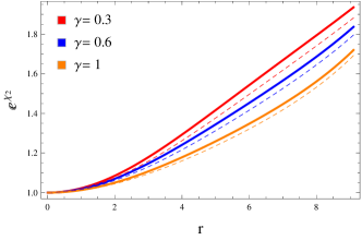
Refer to caption
Figure 1: Deformed grโ€‹rsubscript๐‘”๐‘Ÿ๐‘Ÿg_{rr} metric function (41) versus r๐‘Ÿr (in km) for ๐’ฎยฏ=0.1ยฏ๐’ฎ0.1\bar{\mathcal{S}}=0.1 (solid lines) and ๐’ฎยฏ=0.8ยฏ๐’ฎ0.8\bar{\mathcal{S}}=0.8 (dashed lines) corresponding to ฮ ยฏ=0ยฏฮ 0\bar{\Pi}=0.

We adopt the fโ€‹(โ„,๐•‹)๐‘“โ„๐•‹f(\mathbb{R},\mathbb{T}) model (11) to discuss the graphical interpretation of the both resulting charged solutions, their corresponding deformation functions as well as the complexity factors. For the first solution, different values of the decoupling parameter and charge along with an integration constant โ„‚1=โˆ’0.003subscriptโ„‚10.003\mathbb{C}_{1}=-0.003 and ฯ‡3=0.3subscript๐œ’30.3\chi_{3}=0.3 are chosen so that the corresponding physical characteristics can be explored. Figure 1 assures an acceptable (singularity free and increasing outwards) behavior of the deformed grโ€‹rsubscript๐‘”๐‘Ÿ๐‘Ÿg_{rr} potential (41) for 0<r<โ„›0๐‘Ÿโ„›0<r<\mathcal{R}. A resulting model would be found acceptable only if the governing state parameters representing interior distribution (like the energy density and pressure) are maximum (minimum) and positively finite at the center (boundary) of an astrophysical body. Figure 2 depicts such behavior for the first solution being represented by Eqs.(43)-(46). The upper left plot of the energy density shows its maximum value in the starโ€™s core. However, the increment in the decoupling parameter as well as an electric charge decreases the density of the fluid. On the other hand, the pressure in radial and transverse directions shows the opposite behavior to that of the density corresponding to the parameter ฮณ๐›พ\gamma. Additionally, the pressure components decrease with the increment in an electric charge. The starโ€™s boundary contains only the tangential pressure while the radial one disappears at that point. Figure 2 (last plot) also exhibits the plot of the anisotropic factor that vanishes only at the core for ฮณ=0.3,0.6๐›พ0.30.6\gamma=0.3,~{}0.6 and throughout for ฮณ=1๐›พ1\gamma=1. Hence, the isotropization of the developed solution is clearly observed from the graphical analysis.
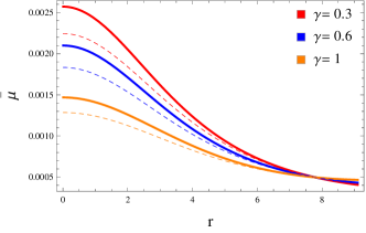
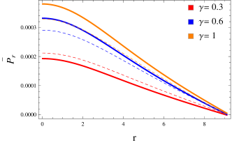
Refer to caption
Refer to caption
Refer to caption
Refer to caption
Figure 2: Matter determinants and anisotropy (in km-2) versus r๐‘Ÿr (in km) for ๐’ฎยฏ=0.1ยฏ๐’ฎ0.1\bar{\mathcal{S}}=0.1 (solid lines) and ๐’ฎยฏ=0.8ยฏ๐’ฎ0.8\bar{\mathcal{S}}=0.8 (dashed lines) corresponding to ฮ ยฏ=0ยฏฮ 0\bar{\Pi}=0.
Refer to caption
Refer to caption
Refer to caption
Figure 3: Mass (in km), compactness and redshift versus r๐‘Ÿr (in km) for ๐’ฎยฏ=0.1ยฏ๐’ฎ0.1\bar{\mathcal{S}}=0.1 (solid lines) and ๐’ฎยฏ=0.8ยฏ๐’ฎ0.8\bar{\mathcal{S}}=0.8 (dashed lines) corresponding to ฮ ยฏ=0ยฏฮ 0\bar{\Pi}=0.
Refer to caption
Refer to caption
Figure 4: Dominant energy conditions (in km-2) versus r๐‘Ÿr (in km) for ๐’ฎยฏ=0.1ยฏ๐’ฎ0.1\bar{\mathcal{S}}=0.1 (solid lines) and ๐’ฎยฏ=0.8ยฏ๐’ฎ0.8\bar{\mathcal{S}}=0.8 (dashed lines) corresponding to ฮ ยฏ=0ยฏฮ 0\bar{\Pi}=0.
Refer to caption
Refer to caption
Refer to caption
Figure 5: Radial/tangential sound speeds and cracking criteria versus r๐‘Ÿr (in km) for ๐’ฎยฏ=0.1ยฏ๐’ฎ0.1\bar{\mathcal{S}}=0.1 (solid lines) and ๐’ฎยฏ=0.8ยฏ๐’ฎ0.8\bar{\mathcal{S}}=0.8 (dashed lines) corresponding to ฮ ยฏ=0ยฏฮ 0\bar{\Pi}=0.

Figure 3 presents the mass function of the corresponding spherical self-gravitating model. We find the charged/uncharged isotropic system to be less dense in comparison with the respective anisotropic analog. Moreover, we calculate the resulting mass at the spherical boundary in terms of mass of the sun for all parametric choices and deduced that this model fits best with the observational mass for ฮณ=0.3๐›พ0.3\gamma=0.3 and ๐’ฎยฏ=0.1ยฏ๐’ฎ0.1\bar{\mathcal{S}}=0.1, i.e., โ„ณยฏ=1.56โ€‹Mโจ€ยฏโ„ณ1.56subscript๐‘€โจ€\bar{\mathcal{M}}=1.56M_{\bigodot}. The other two parameters plotted in the same Figure guarantee the fulfillment of their respective criteria. The positive trend shown by the state variables (in Figure 2) allows us to plot only the dominant energy conditions such as ฮผยฏโˆ’Pยฏr+s24โ€‹ฯ€โ€‹r4โ‰ฅ0ยฏ๐œ‡subscriptยฏ๐‘ƒ๐‘Ÿsuperscripts24๐œ‹superscript๐‘Ÿ40\bar{\mu}-\bar{P}_{r}+\frac{\mathrm{s}^{2}}{4\pi r^{4}}\geq 0 and ฮผยฏโˆ’PยฏโŠฅโ‰ฅ0ยฏ๐œ‡subscriptยฏ๐‘ƒbottom0\bar{\mu}-\bar{P}_{\bot}\geq 0. These bounds can be seen in Figure 4 from which the viability of the resulting model is revealed. Moreover, multiple strategies are used in Figure 5 to check whether our solution is stable or unstable. The upper two plots provide that ฮณ=0.6๐›พ0.6\gamma=0.6 (with ๐’ฎยฏ=0.1ยฏ๐’ฎ0.1\bar{\mathcal{S}}=0.1 and 0.80.80.8) is the only parametric value for which both sound speeds show stable behavior. Contrariwise, we get the stable model for every choice of ฮณ๐›พ\gamma through the cracking criteria (lower plot). Figure 6 exhibits that the modified scalar factors (51) and (62) decrease and increase, respectively, by increasing the decoupling parameter. However, both factors are in an inverse relation with an electric charge. Further, we compare the behavior of this factor with that of ๐”พโ€‹โ„๐”พโ„\mathbb{GR} and deduce that the complexity reduces in the former case.
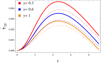
Refer to caption
Refer to caption
Figure 6: Complexity factors (51) and (62) (in km-2) versus r๐‘Ÿr (in km) for ๐’ฎยฏ=0.1ยฏ๐’ฎ0.1\bar{\mathcal{S}}=0.1 (solid lines) and ๐’ฎยฏ=0.8ยฏ๐’ฎ0.8\bar{\mathcal{S}}=0.8 (dashed lines).

The physical properties of the second solution corresponding to ๐•ยฏTโ€‹F=0subscriptยฏ๐•๐‘‡๐น0\bar{\mathbb{Y}}_{TF}=0 is now explored for the same values of ฮณ๐›พ\gamma and ฯ‡3subscript๐œ’3\chi_{3} along with โ„‚3=โˆ’0.001subscriptโ„‚30.001\mathbb{C}_{3}=-0.001. Figure 7 shows that the deformed grโ€‹rsubscript๐‘”๐‘Ÿ๐‘Ÿg_{rr} component possesses singularity-free and increasing nature. The plots of the matter triplet (provided in Eqs.(66)-(68)) and anisotropic factor are demonstrated in Figure 8. They own the same trend as already observed for the first solution. The last plot exhibits that the core (boundary) of a compact star contains no (maximum) anisotropy for all chosen parametric values. However, the increment in charge results in less anisotropy. Figure 9 indicates that the greater the value of ฮณ๐›พ\gamma and charge, the less the mass of a compact star is. Further, the required criteria for the redshift and compactness parameters is fulfilled, as can be seen from the same Figure. The plots in Figure 10 guarantee that the corresponding solution is viable. Figure 11 reveals that our resulting model (66)-(68) is stable for all parametric choices except ฮณ=1๐›พ1\gamma=1 (upper left plot).

Refer to caption
Figure 7: Deformed grโ€‹rsubscript๐‘”๐‘Ÿ๐‘Ÿg_{rr} metric function (65) versus r๐‘Ÿr (in km) for ๐’ฎยฏ=0.1ยฏ๐’ฎ0.1\bar{\mathcal{S}}=0.1 (solid lines) and ๐’ฎยฏ=0.8ยฏ๐’ฎ0.8\bar{\mathcal{S}}=0.8 (dashed lines) corresponding to ๐•ยฏTโ€‹F=0subscriptยฏ๐•๐‘‡๐น0\bar{\mathbb{Y}}_{TF}=0.
Refer to caption
Refer to caption
Refer to caption
Refer to caption
Figure 8: Matter determinants and anisotropy (in km-2) versus r๐‘Ÿr (in km) for ๐’ฎยฏ=0.1ยฏ๐’ฎ0.1\bar{\mathcal{S}}=0.1 (solid lines) and ๐’ฎยฏ=0.8ยฏ๐’ฎ0.8\bar{\mathcal{S}}=0.8 (dashed lines) corresponding to ๐•ยฏTโ€‹F=0subscriptยฏ๐•๐‘‡๐น0\bar{\mathbb{Y}}_{TF}=0.
Refer to caption
Refer to caption
Refer to caption
Figure 9: Mass (in km), compactness and redshift versus r๐‘Ÿr (in km) for ๐’ฎยฏ=0.1ยฏ๐’ฎ0.1\bar{\mathcal{S}}=0.1 (solid lines) and ๐’ฎยฏ=0.8ยฏ๐’ฎ0.8\bar{\mathcal{S}}=0.8 (dashed lines) corresponding to ๐•ยฏTโ€‹F=0subscriptยฏ๐•๐‘‡๐น0\bar{\mathbb{Y}}_{TF}=0.
Refer to caption
Refer to caption
Figure 10: Dominant energy conditions (in km-2) versus r๐‘Ÿr (in km) for ๐’ฎยฏ=0.1ยฏ๐’ฎ0.1\bar{\mathcal{S}}=0.1 (solid lines) and ๐’ฎยฏ=0.8ยฏ๐’ฎ0.8\bar{\mathcal{S}}=0.8 (dashed lines) corresponding to ๐•ยฏTโ€‹F=0subscriptยฏ๐•๐‘‡๐น0\bar{\mathbb{Y}}_{TF}=0.
Refer to caption
Refer to caption
Refer to caption
Figure 11: Radial/tangential sound speeds and cracking criteria versus r๐‘Ÿr (in km) for ๐’ฎยฏ=0.1ยฏ๐’ฎ0.1\bar{\mathcal{S}}=0.1 (solid lines) and ๐’ฎยฏ=0.8ยฏ๐’ฎ0.8\bar{\mathcal{S}}=0.8 (dashed lines) corresponding to ๐•ยฏTโ€‹F=0subscriptยฏ๐•๐‘‡๐น0\bar{\mathbb{Y}}_{TF}=0.

7 Conclusions

This paper explores the existence of self-gravitating spherical anisotropic charged models by extending the original solutions to an additional matter field by using the strategy of gravitational decoupling in fโ€‹(โ„,๐•‹)=โ„+2โ€‹ฯ‡3โ€‹๐•‹๐‘“โ„๐•‹โ„2subscript๐œ’3๐•‹f(\mathbb{R},\mathbb{T})=\mathbb{R}+2\chi_{3}\mathbb{T} theory. We initially added the Lagrangian densities of the electromagnetic field and extra source in the action and formulated the corresponding field equations. We then separated the effects of the seed and extra matter sources by dividing the field equations into two individual sets by employing the MGD scheme. The influence of the charge has only been observed in the field equations representing the original matter distribution. Two different solutions to this set were obtained by taking the following ansatz

ฯ‡1โ€‹(r)=lnโก{๐’ž22โ€‹(1+r2๐’ž12)},ฯ‡5โ€‹(r)=eโˆ’ฯ‡2โ€‹(r)=๐’ž12+r2๐’ž12+3โ€‹r2,formulae-sequencesubscript๐œ’1๐‘Ÿsuperscriptsubscript๐’ž221superscript๐‘Ÿ2superscriptsubscript๐’ž12subscript๐œ’5๐‘Ÿsuperscript๐‘’subscript๐œ’2๐‘Ÿsuperscriptsubscript๐’ž12superscript๐‘Ÿ2superscriptsubscript๐’ž123superscript๐‘Ÿ2\chi_{1}(r)=\ln\bigg{\{}\mathcal{C}_{2}^{2}\bigg{(}1+\frac{r^{2}}{\mathcal{C}_{1}^{2}}\bigg{)}\bigg{\}},\quad\chi_{5}(r)=e^{-\chi_{2}(r)}=\frac{\mathcal{C}_{1}^{2}+r^{2}}{\mathcal{C}_{1}^{2}+3r^{2}},

and Tolman IV spacetime, respectively. These metric potentials contain a triplet (๐’ž1,๐’ž2,๐’ž3subscript๐’ž1subscript๐’ž2subscript๐’ž3\mathcal{C}_{1},\mathcal{C}_{2},\mathcal{C}_{3}) as unknown quantities whose values have been calculated through continuity of the metric potentials at the spherical boundary. The other set (25)-(27) encoding the effect of the additional source was then solved by employing some constraints on โ„ญฮฒโ€‹ฮฑsubscriptโ„ญ๐›ฝ๐›ผ\mathfrak{C}_{\beta\alpha}. We have constructed an isotropic model from being anisotropic for a particular value, i.e., ฮณ=1๐›พ1\gamma=1, leading to the first solution. Further, the second model was developed by taking into consideration that the resultant complexity factor corresponding to both matter sectors becomes null.

Different values of the decoupling parameter along with fixed values of the coupling as well as integration constants have been chosen to graphically analyze the developed solutions so that we can check how ฮณ๐›พ\gamma influences these extended models. The matter determinants for both solutions (presented in (43)-(45) and (66)-(68)), their corresponding anisotropic factors, redshift, compactness and the energy conditions have shown an acceptable behavior. It was also observed that the first resulting model corresponding to ฮ ยฏ=0ยฏฮ 0\bar{\Pi}=0 possesses a dense interior for every value of ฮณ๐›พ\gamma in comparison with the second solution. Further, the radial metric components (41) and (65) have been deformed and plotted which exhibit positive and increasing behavior throughout (Figures 1 and 7). We have employed the causality and cracking criteria to analyze whether the modified models show stable behavior for all choices of the decoupling parameter and charge or not. We have observed that the first model is stable only for ฮณ=0.6๐›พ0.6\gamma=0.6 through the causality conditions, and thus compatible with the uncharged fโ€‹(โ„,๐•‹)๐‘“โ„๐•‹f(\mathbb{R},\mathbb{T}) framework [9] as well as Brans-Dicke theory only for this value [47]. However, the cracking criterion provides both stable solutions. Eventually, all these results can be reduced to ๐”พโ€‹โ„๐”พโ„\mathbb{GR} for ฯ‡3=0subscript๐œ’30\chi_{3}=0.

Data Availability Statement: No Data associated in the manuscript.

Conflict of Interest Statement: The authors declare that there is no conflict of interest.

References

  • [1] Capozziello, S. et al.: Class. Quantum Grav. 25(2008) 085004; Nojiri, S. et al.: Phys. Lett. B 681(2009)74.
  • [2] de Felice, A. and Tsujikawa, S.: Living Rev. Relativ. 13(2010)3; Nojiri, S. and Odintsov, S.D.: Phys. Rep. 505(2011)59.
  • [3] Sharif, M. and Kausar, H.R.: J. Cosmol. Astropart. Phys. 07(2011)022.
  • [4] Astashenok, A.V., Capozziello, S. and Odintsov, S.D.: J. Cosmol. Astropart. Phys. 01(2015)001; Phys. Lett. B 742(2015)160.
  • [5] Bertolami, O. et al.: Phys. Rev. D 75(2007)104016.
  • [6] Harko, T. et al.: Phys. Rev. D 84(2011)024020.
  • [7] Houndjo, M.J.S.: Int. J. Mod. Phys. D 21(2012)1250003.
  • [8] Das, A. et al.: Phys. Rev. D 95(2017)124011.
  • [9] Sharif, M. and Naseer, T.: Eur. Phys. J. Plus 137(2022)1304.
  • [10] Azmat, H. and Zubair M.: Eur. Phys. J. Plus 136(2018)112.; Rej, P., Bhar, Piyali. and Govender, M.: Eur. Phys. J. C 81(2021)316; Zubair, M. et al.: New Astron. 88(2021)101610.
  • [11] Shamir, M.F., Asghar, Z. and Malik, A.: Fortschr. Phys. 70(2022)2200134; Malik, A., Yousaf, Z., Jan, M., Shahzad, M.R. and Akram, Z.: Int. J. Geom. Methods Mod. 20(2023)2350061.
  • [12] Koussour, M. and Bennai, M.: Int. J. Geom. Methods Mod. 19(2022)2250038; Myrzakulov, N., Koussour, M., Alfedeel, A.H.A. and Hassan, E.I.: Chin. Phys. C (2023) 10.1088/1674-1137/acf2fa.
  • [13] Bora, J. and Goswami, U.D.: Phys. Dark Universe 38(2022)101132; Pretel, J.M.Z.: Mod. Phys. Lett. A 37(2022)2250188.
  • [14] Pappas, T.D., Posada, C. and Stuchlรญk, Z.: Phys. Rev. D 106(2022)124014; Nashed, G.G.L.: Astrophys. J. 950(2023)129.
  • [15] Malik, A., Asghar, Z. and Shamir, M.F.: New Astron. 104(2023)102071; Asghar, Z., Shamir, M.F., Usman, A. and Malik, A.: Chin. J. Phys. 83(2023)427.
  • [16] Harko, T. et al.: Phys. Rev. D 84(2011)024020.
  • [17] Carvalho, G.A. et al.: Eur. Phys. J. C 77(2017)871.
  • [18] Ordines, T.M. and Carlson, E.D.: Phys. Rev. D 99(2019)104052.
  • [19] Carvalho, G.A. et al.: Eur. Phys. J. C 77(2017)871.
  • [20] Velten, H. and Caramรชs, T.R.P.: Phys. Rev. D 95(2017)123536.
  • [21] Bhattacharjee, S. and Sahoo, P.K.: Grav. Cosmol. 26(2020)281.
  • [22] Ashmita, Sarkar, P. and Das, P.K.: Int. J. Mod. Phys. D 31(2022)2250120.
  • [23] Kaur, S., Maurya, S.K., Shukla, S. and Nag, R.: Chin. J. Phys. 77(2022)2854.
  • [24] Ovalle, J.: Mod. Phys. Lett. A 23(2008)3247.
  • [25] Ovalle, J. and Linares, F.: Phys. Rev. D 88(2013)104026.
  • [26] Casadio, R., Ovalle, J. and Da Rocha, R.: Class. Quantum Grav. 32(2015)215020.
  • [27] Ovalle, J. et al.: Eur. Phys. J. C 78(2018)960.
  • [28] Sharif, M. and Sadiq, S.: Eur. Phys. J. C 78(2018)410.
  • [29] Gabbanelli, L., Rincรณn, ร. and Rubio, C.: Eur. Phys. J. C 78(2018)370.
  • [30] Estrada, M. and Tello-Ortiz, F.: Eur. Phys. J. Plus 133(2018)453.
  • [31] Hensh, S. and Stuchlรญk, Z.: Eur. Phys. J. C 79(2019)834.
  • [32] Sharif, M. and Majid, A.: Chin. J. Phys. 68(2020)406.
  • [33] Sharif, M. and Naseer, T.: Phys. Scr. 97(2022)055004; Int. J. Mod. Phys. D 31(2022)2240017; Pramana 96(2022)119.
  • [34] Bekenstein, J.D.: Phys. Rev. D 4(1971)2185.
  • [35] Esculpi, M. and Aloma, E.: Eur. Phys. J. C 67(2010)521.
  • [36] de Felice, F., Yu, Y.Q. and Fang, J.: Mon. Not. R. Astron. Soc. 277(1995)L17.
  • [37] de Felice, F., Liu, S.M. and Yu, Y.Q.: Class. Quantum Gravit. 16(1999)2669.
  • [38] Pretel, J.M.Z., Tangphati, T., Banerjee, A. and Pradhan, A.: Chin. Phys. C 46(2022)115103.
  • [39] Sharif, M. and Naseer, T.: Chin. J. Phys. 73(2021)179; ibid. 81(2023)37; ibid. 85(2023)41; Phys. Scr. 97(2022)125016; Indian J. Phys. 96(2022)4373; Fortschr. Phys. 71(2023)2200147.
  • [40] Herrera, L.: Phys. Rev. D 97(2018)044010.
  • [41] Herrera, L., Di Prisco, A. and Ospino, J.: Phys. Rev. D 98(2018)104059.
  • [42] Yousaf, Z., Bhatti, M.Z. and Naseer, T.: Eur. Phys. J. Plus 135(2020)353; Phys. Dark Universe 28(2020)100535; Int. J. Mod. Phys. D 29(2020)2050061; Ann. Phys. 420(2020)168267.
  • [43] Yousaf, Z. et al.: Phys. Dark Universe 29(2020)100581; Yousaf, Z. et al.: Mon. Not. R. Astron. Soc. 495(2020)4334; Sharif, M. and Naseer, T.: Chin. J. Phys. 77(2022)2655; Eur. Phys. J. Plus 137(2022)947.
  • [44] Carrasco-Hidalgo, M. and Contreras, E.: Eur. Phys. J. C 81(2021)757; Andrade, J. and Contreras, E.: Eur. Phys. J. C 81(2021)889; Arias, C. et al.: Ann. Phys. 436(2022)168671; Sharif, M. and Naseer, T.: Ann. Phys. 453(2023)169311; Phys. Dark Universe 42(2023)101324.
  • [45] Casadio, R. et al.: Eur. Phys. J. C 79(2019)826.
  • [46] Maurya, S.K. and Nag, R.: Eur. Phys. J. C 82(2022)48; Maurya, S.K. et al.: Eur. Phys. J. C 82(2022)100.
  • [47] Sharif, M. and Majid, A.: Eur. Phys. J. Plus 137(2022)114.
  • [48] Sharif, M. and Naseer, T.: Class. Quantum Gravit. 40(2023)035009; Naseer, T. and Sharif, M.: Fortschr. Phys. 71(2023)2300004.
  • [49] Einstein, A.: Ann. Math. 40(1939)922.
  • [50] Gรผver, T., Wroblewski, P., Camarota, L. and ร–zel, F.: Astrophys. J. 719(2010)1807.
  • [51] Buchdahl, H.A.: Phys. Rev. 116(1959)1027.
  • [52] Ivanov, B.V.: Phys. Rev. D 65(2002)104011.
  • [53] Abreu, H., Hernandez, H. and Nunez, L.A.: Class. Quantum Gravit. 24(2007)4631.
  • [54] Herrera, L.: Phys. Lett. A 165(1992)206; Phys. Rev. D 101(2020)104024.
  • [55] Malik, A., Shafaq, A., Naz, T. and Al-khaldi, A.H.: Eur. Phys. J. C 83(2023)765.