Dual-VQE: A quantum algorithm to lower bound the ground-state energy
Abstract
The variational quantum eigensolver (VQE) is a hybrid quantum–classical variational algorithm that produces an upper-bound estimate of the ground-state energy of a Hamiltonian. As quantum computers become more powerful and go beyond the reach of classical brute-force simulation, it is important to assess the quality of solutions produced by them. Here we propose a dual variational quantum eigensolver (dual-VQE) that produces a lower-bound estimate of the ground-state energy. As such, VQE and dual-VQE can serve as quality checks on their solutions; in the ideal case, the VQE upper bound and the dual-VQE lower bound form an interval containing the true optimal value of the ground-state energy. The idea behind dual-VQE is to employ semi-definite programming duality to rewrite the ground-state optimization problem as a constrained maximization problem, which itself can be bounded from below by an unconstrained optimization problem to be solved by a variational quantum algorithm. When using a convex combination ansatz in conjunction with a classical generative model, the quantum computational resources needed to evaluate the objective function of dual-VQE are no greater than those needed for that of VQE. We simulated the performance of dual-VQE on the transverse-field Ising model, and found that, for the example considered, while dual-VQE training is slower and noisier than VQE, it approaches the true value with error of order .
Introduction—A key approach hoped to achieve quantum advantage on near-term quantum computers involves the use of variational quantum algorithms [5, 14]. The variational quantum eigensolver (VQE) was the first such algorithm proposed [36]: it estimates an upper bound on the ground-state energy of a Hamiltonian. The basic idea behind it is simple, based on the well known variational principle from physics [22]. For a Hamiltonian , its ground-state energy is equal to its minimum eigenvalue , which is equal to the following minimization problem:
| (1) |
where is the set of density matrices (positive semi-definite matrices with trace equal to one). Since the objective function is linear in and the set of density matrices is convex, the optimal value of (1) is obtained on the boundary of the set (i.e., the set of pure states). It then follows that
| (2) |
where is the set of state vectors. In a variational approach, the set of pure states is approximated by a parameterized set of states, where is a parameter set and is a parameter vector. The equality in (2) is preserved if the set of parameterized pure states contains an optimal pure state. In reality, guaranteeing this condition is not possible, leading to the following upper bound on the ground-state energy:
| (3) |
An example of wide interest is when and is a Hermitian matrix, describing the local interactions that take place between spin-1/2 particles. In this case, , where each is a Hermitian matrix of constant size that acts non-trivially on a constant number of particles. Observing that the optimization in (1) is a semi-definite program (SDP) [40], one could attempt to solve it by means of well known approaches used to solve SDPs; however, the computational complexity of such approaches is exponential in and thus infeasible. Standard classical approaches for solving (1) in the general case suffer from the same problem, or they avoid it by not allowing for the optimization to include highly entangled states (see [18] for a review of some of these methods).
VQE instead parameterizes the set of state vectors by a parameterized quantum circuit acting on an easily preparable initial state , leading to , and measures the expectation of each observable with respect to in order to obtain an estimate of . Then the sum is an estimate of the desired expectation . The estimates of and its gradient can be fed to a classical optimization procedure and this process iterated until convergence or a maximum number of iterations is reached. As a consequence of (3), this procedure in the ideal case produces an estimate of an upper bound for the ground-state energy .
In the short term, while classical computers are still competitive with small-scale quantum computers, it is possible to test how well VQE is performing by comparing its value with an extremely precise estimate of the true known value. As mentioned above, an SDP can output such a precise estimate for sufficiently small system sizes. However, this approach is not viable in the long term, which leads to the key question that our paper addresses:
How can we assess the quality of VQE’s upper-bound estimate of without access to a reliable classical algorithm for estimating ?
We address this question by developing a variational quantum algorithm (called dual-VQE) to estimate a lower bound on the ground-state energy, which can be compared to the upper-bound estimate obtained from VQE. Since the two estimates ideally sandwich the true optimal value, they serve as quality checks on each other. The key ideas of our approach are to 1) use SDP duality theory to reformulate as a maximization problem and 2) further reformulate this maximization problem in such a way that it can be estimated by means of a variational quantum algorithm, which finally leads to a lower-bound estimate of . We call our method dual-VQE because it makes use of the dual characterization of to arrive at this lower-bound estimate. After executing VQE and dual-VQE, one can then compare the upper-bound and lower-bound estimates to understand how well a quantum computer can approximate the true optimal value , without the aid of precise classical methods.
The dual-VQE method involves 1) converting inequality constraints to equality constraints by means of positive semi-definite slack variables, 2) converting a constrained optimization into an unconstrained one by means of a penalty term in the objective function, 3) replacing positive semi-definite slack variables with scaled parameterized quantum states that are efficiently preparable on quantum computers, and 4) estimating various terms in the objective function by means of the destructive swap test [21] and sampling estimates of expectations of observables. Our companion paper [17] explores this general approach in a much broader context beyond the ground-state energy problem.
Although there have been various classical algorithms proposed for obtaining lower bounds on the ground-state energy [28, 29, 30, 8, 23], they all ultimately suffer from the exponential increase of the space on which acts, as the number of particles increases. Our approach is fundamentally different, involving a reformulation of the original optimization problem in terms of its SDP dual, and then bounding that quantity from below using a variational quantum algorithm. Our approach is also complementary to [9, Section VI-A], which does not take a variational approach, nor does it provably obtain a lower bound on the ground-state energy.
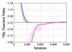
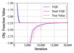
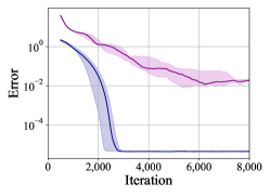
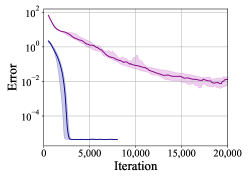
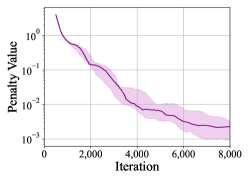
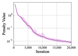
The rest of our paper proceeds by detailing the dual-VQE method outlined above, and then we report the results of simulations of the transverse-field Ising model, a key example of physical interest. We find that the dual-VQE approach on a two-qubit example takes more iterations to converge as compared to the standard VQE optimization; however, it approaches the true value with error on the order of . We also note that in this example, the objective function values across training are noisier for dual-VQE when compared to VQE. We expect this behavior due to the increase in number of terms and parameters when estimating the ground-state energy with dual-VQE. Details of numerical simulations are given below, and training plots are shown in Figure 1.
Dual-VQE theoretical derivation—Let us first use some basic SDP duality theory to derive a well known result, that the following weak-duality inequality holds:
| (4) |
where is the SDP dual of (1). Note that actually equality holds in (4) due to Slater’s theorem [13]: we can pick , where is the dimension of the underlying Hilbert space, and as strictly feasible choices in both the dual and primal, thus satisfying the conditions of Slater’s theorem. Recall that the matrix inequality holds for Hermitian matrices and if is a positive semi-definite matrix. Then consider that
| (5) | ||||
| (6) | ||||
| (7) | ||||
| (8) | ||||
| (9) |
The second equality follows by introducing the Lagrange multiplier and because the constraint does not hold if and only if . The third equality holds by simple algebra. The sole inequality follows from the standard max-min inequality. The final equality follows by thinking of as a matrix Lagrange multiplier and because the constraint does not hold if and only if .
Now that we have recalled this standard result, let us focus on showing how to estimate the lower bound in (4) on a quantum computer. Recalling that the matrix inequality is equivalent to the existence of a positive semi-definite matrix such that , we conclude that
| (10) |
The matrix is known in the theory of optimization [13] as a slack variable because it eliminates the slack in the inequality constraint by reducing it to an equality constraint.
Our next observation is that every positive semi-definite matrix can be written as a scaled density matrix, i.e., , where and , implying that
| (11) |
Next, we adopt a standard approach of introducing a penalty term in the objective function to transform the constrained optimization to an unconstrained one:
| (12) |
where is a penalty parameter and is the Hilbert–Schmidt norm of a matrix . Note that the equality in (12) holds whenever the penalty term is faithful (specifically, we invoke [6, Proposition 5.2.1] to justify this conclusion, setting therein for all ). By faithfulness, we mean that the penalty term is equal to zero if and only if . This is true for the Hilbert–Schmidt norm, and this particular norm has the convenient advantage that it can be estimated by quantum sampling procedures that we recall below.
The final step is to modify the optimization in (12) to be over a parameterized set of density matrices instead of being over all density matrices, which implies that
| (13) |
Piecing together all these steps in (4)–(13), expanding the Hilbert-Schmidt norm, and defining
| (14) |
where is a parameter set,
| (15) |
and is a penalty parameter, we obtain the main theoretical result supporting the dual-VQE approach:
Theorem 1 (Dual-VQE lower bound)
The function in (14) provides a lower bound on the ground-state energy of the Hamiltonian in the limit ; i.e.,
| (16) |
Inspecting (15), only two terms and depend on the optimization variable , while constant terms like and (having no dependence on , , or ) can be calculated offline.
A key case of interest for physics and chemistry is when is a linear combination of Pauli strings, so that
| (17) |
where , , is a Pauli string, and , , , and are the standard Pauli matrices. For this case, it follows from substitution and the orthogonality relation that
| (18) | ||||
| (19) | ||||
| (20) |
As in the common Hamiltonian models for physics and chemistry, the number of non-zero coefficients in the set is polynomial in, so that the objective function in (15) can be efficiently estimated.
Dual-VQE algorithm for lower bounding the ground-state energy—The basic idea behind the dual-VQE algorithm is to follow the standard penalty method [6, Section 5.2]: define a sequence of optimization problems where is a monotone increasing sequence of penalty parameters. We then solve the optimization for each and use the solution as the initial guess for the next iteration. Under the assumption that each optimization can be solved, the method is guaranteed to converge to the correct solution. In our simulations, we used a constant value of the penalty parameter and found that it performs well in practice.
In dual-VQE, we estimate the expectation by sampling from a quantum computer, and we use other approaches, either quantum or classical, for estimating the purity . If employing gradient descent for solving each optimization, one should estimate the gradient as well, which we discuss further below. The main additional overhead compared to VQE is the need to employ an ansatz for generating a mixed state and to estimate the purity , given that VQE already estimates a term like . However, as we discuss below, one approach reduces the estimation of the purity to a classical sampling task, thus removing the need for a quantum computer for this part.
There are at least two general ways of parameterizing the set of mixed states, called the purification ansatz [16, 35, 19] and the convex combination ansatz [46, 26, 19, 41]. Focusing on the first one to start, it is based on the purification principle [12, 44, 45], in which every mixed state is realized as the marginal of a pure state on a larger system. For the purification ansatz, we simply start with a parameterized family of pure states of a reference system and the system of interest, and then we obtain a parameterized family of mixed states via the partial trace . We can estimate the purity by means of the destructive swap test [21] (see, e.g., [11, Section 2.2] for a precise statement of the algorithm). We can estimate the gradient of the objective function in (16) by means of the parameter-shift rule [27, 33, 39], simply because
| (21) |
and one can also use a slightly modified version of the parameter-shift rule along with the destructive swap test to estimate the gradient of the purity term because
| (22) |
where
| (23) |
is the unitary and Hermitian swap operator, and we have suppressed system labels in (22) for brevity (see also [19, Eq. (C2)] in this context).
The convex combination ansatz is based on the fact that every mixed state can be written as a convex combination of pure orthogonal states. Following this idea, we obtain a parameterized family by separately parameterizing the eigenvalues and eigenvectors as follows:
| (24) |
where is a parameterized probability distribution, is a parameterized unitary, and is the standard computational basis. The parameterized probability distribution can be realized by a neural-network-based generative model [2, 10, 34] or a quantum circuit Born machine [7], while the parameterized unitary can be realized by a parameterized circuit.
Interestingly, although it is necessary to use a quantum computer to estimate the purity for the purification ansatz, it is not necessary to do so when using the convex combination ansatz in conjunction with a neural-network-based generative model: it suffices to employ a classical sampling approach, thus further reducing the quantum resource requirements for dual-VQE (see also [19, Eqs. (20)–(23)] in this context). This is because , so that one can repeatedly sample from and perform a collision test to estimate . Thus, for the convex combination ansatz used in the aforementioned way, one only needs a quantum computer to estimate the expectation
| (25) |
which can be done by repeating the following procedure and calculating the sample mean: take a sample from , prepare the state , measure this state according to , and record the outcome. To estimate the gradient of the purity and the gradient of the expectation with respect to , perhaps the simplest approach is to use the simultaneous perturbation stochastic approximation [42], because the distribution in this case is not differentiable, and as such, standard methods like backpropagation are not readily applicable (see [10] for further discussions and other approaches).
| Purification ansatz | Convex-combination ansatz | |
|---|---|---|
| Objective function |
|
|
| Error |
|
|
| Penalty value |
|
|
Results of numerical simulations—We now present the results of simulations that test the performance of dual-VQE on the transverse field Ising model, described by the following Hamiltonian of qubits:
| (26) |
where tensor products with identities are left implicit, is an interaction strength, and is related to the strength of the external field. In particular, we showcase our algorithm on the following two-qubit example problem instance:
| (27) |
Prior to training, we initialized the parameters , , and . We set the parameters and in (12) to be equal to zero and one, respectively. We selected the components of the initial parameter vector for the state uniformly at random from . The optimal state is almost always a full-rank mixed state. Thus, we used either a three-layer purification ansatz or a convex-combination ansatz with a two-layer quantum circuit Born machine and a two-layer unitary. The particular structure of the purification ansatz and the quantum circuit Born machine we use can be found in a figure in our companion paper [17].
In addition to setting the initializations of the parameters of our optimization, we assigned specific values to the hyperparameters. We chose the penalty parameter to have a constant value of throughout training, and we implemented a decreasing learning rate scheme. We initialized the learning rate to a maximum value of , and every iterations, we checked whether the objective function value decreased three times in a row over the past iterations. In this case, we reduced the learning rate by a factor of two. We repeated this process until a minimum value of was met.
Training crucially depends on estimating the gradient, which allows us to pick the next set of parameters. We used the SPSA algorithm [42], which provides an unbiased estimate of the gradient at each step. We chose this method as the per-iteration cost of this algorithm is constant in the number of parameters, and we found that it works well in practice. If the norm of the gradient had a value greater than one, we normalized the gradient before performing the update step of gradient descent. We found that this prevents immediate divergence due to a potentially high initial penalty value. It also allowed us to use higher values of the learning rate than we would have been able to otherwise. Training concluded when an arbitrarily set maximum number of iterations was met.
The results of the simulations are displayed in Figure 1. In these plots, solid lines depict results of both the standard VQE algorithm (with fixed learning rate of and gradient estimated by normalized SPSA) and our dual-VQE approach. The solid lines show median values across ten independent runs, and the shading is the interquartile range. The dashed line is the true value of the ground-state energy estimated via the SDP. The variation displayed in the graphs comes from three sources of randomness: the randomized initializations of all parameterized quantum circuits, randomness in the SPSA algorithm for gradient estimation, and shot noise over shots for every measurement of a quantum circuit. In our simulations, we were able to achieve an error of order after iterations of training. These results give evidence that using VQE and dual-VQE allows us to bound the true value from both above and below, respectively, as desired.
Discussion and conclusion—In conclusion, we proposed dual-VQE as a variational quantum algorithm for lower bounding the ground-state energy of a Hamiltonian. This lower bound can be compared with the upper bound obtained from the traditional VQE method, and the two bounds serve as quality checks on each other that ideally determine an interval containing the optimal ground-state energy. As discussed above, the quantum computational resources required for evaluating the objective function of dual-VQE are no greater than those needed for VQE’s objective function when using the convex combination ansatz in conjunction with a classical generative model.
While Theorem 1 guarantees that dual-VQE provides a rigorous lower bound on the ground state energy in the limit , for finite the value provided by dual-VQE is technically an estimate rather than a strict bound. However, our numerical simulations give evidence, for the example considered, that VQE and dual-VQE do indeed bound the optimal ground-state energy from above and below, respectively. Nonetheless, it would be valuable to investigate whether it is possible to obtain bounds on the degree to which deviations are possible for finite . This would allow us to certify the reliability of dual-VQE and serve as a guide to an optimum choice for .
A key issue that plagues variational quantum algorithms is the presence of barren plateaus in the training landscape [31, 20, 37], meaning that the gradient (or equivalently cost differences [1]) vanishes exponentially fast in the number of qubits. This has been shown to occur for highly expressive [24] or highly entangling [32] ansätze or even at low circuit depths for global costs [15]. For local problem Hamiltonians, the only term we need to evaluate on a quantum computer, , is local and hence in such cases, for -depth hardware efficient ansätze, dual-VQE provably avoids barren plateaus [15]. However, a worry here is that such short-depth circuits might also be classically simulable via state-of-the-art methods [43, 4, 25, 3, 38]. An important question for dual-VQE, shared also with other variational quantum algorithms, is thus whether we can identify quantum models that both avoid barren plateaus and cannot be classically simulated. One potential avenue would be to try and find clever initialization strategies to explore small subsections of the landscape that exhibit substantial gradients and are also hard to simulate classically.
For future work, it would certainly be of interest to scale up dual-VQE to much larger systems beyond the reach of brute-force classical simulation and to compare the results of VQE and dual-VQE with each other. We also think it would be worthwhile to pursue other methods, besides the penalty method, for performing the optimization in dual-VQE. A promising approach would be to combine a variational approach with an interior-point method, but for this approach, it seems we would need an efficient method, suitable for near-term quantum computers, for estimating the logarithm of the determinant of a matrix on a quantum computer.
Data availability statement—All source codes used to run the simulations and generate the figures are available as arXiv ancillary files with the arXiv posting of our companion paper [17].
Acknowledgements.
We thank Paul Alsing, Ziv Goldfeld, Daniel Koch, Saahil Patel, and Manuel S. Rudolph for helpful discussions. JC and HW acknowledge support from the Engineering Learning Initiative in Cornell University’s College of Engineering. ZH acknowledges support from the Sandoz Family Foundation Monique de Meuron program for Academic Promotion. IL, TN, DP, SR, and MMW acknowledge support from the School of Electrical and Computer Engineering at Cornell University. TN, DP, SR, and MMW acknowledge support from the National Science Foundation under Grant No. 2315398. DP, SR, and MMW acknowledge support from AFRL under agreement no. FA8750-23-2-0031. This material is based on research sponsored by Air Force Research Laboratory under agreement number FA8750-23-2-0031. The U.S. Government is authorized to reproduced and distribute reprints for Governmental purposes notwithstanding any copyright notation thereon. The views and conclusions contained herein are those of the authors and should not be interpreted as necessarily representing the official policies or endorsements, either expressed or implied, of Air Force Research Laboratory or the U.S. Government. This research was conducted with support from the Cornell University Center for Advanced Computing, which receives funding from Cornell University, the National Science Foundation, and members of its Partner Program.References
- AHCC [22] Andrew Arrasmith, Zoë Holmes, Marco Cerezo, and Patrick J. Coles. Equivalence of quantum barren plateaus to cost concentration and narrow gorges. Quantum Science and Technology, 7(4):045015, 2022.
- AHS [85] David H. Ackley, Geoffrey E. Hinton, and Terrence J. Sejnowski. A learning algorithm for Boltzmann machines. Cognitive Science, 9(1):147–169, 1985.
- ATKZ [23] Sajant Anand, Kristan Temme, Abhinav Kandala, and Michael Zaletel. Classical benchmarking of zero noise extrapolation beyond the exactly-verifiable regime, 2023, 2306.17839.
- BC [23] Tomislav Begušić and Garnet Kin-Lic Chan. Fast classical simulation of evidence for the utility of quantum computing before fault tolerance, 2023, 2306.16372.
- BCLK+ [22] Kishor Bharti, Alba Cervera-Lierta, Thi Ha Kyaw, Tobias Haug, Sumner Alperin-Lea, Abhinav Anand, Matthias Degroote, Hermanni Heimonen, Jakob S. Kottmann, Tim Menke, Wai-Keong Mok, Sukin Sim, Leong-Chuan Kwek, and Alan Aspuru-Guzik. Noisy intermediate-scale quantum (NISQ) algorithms. Reviews of Modern Physics, 94(1):015004, February 2022, 2101.08448.
- Ber [16] Dimitri Bertsekas. Nonlinear Programming. Athena Scientific, third edition, June 2016.
- BGPP+ [19] Marcello Benedetti, Delfina Garcia-Pintos, Oscar Perdomo, Vicente Leyton-Ortega, Yunseong Nam, and Alejandro Perdomo-Ortiz. A generative modeling approach for benchmarking and training shallow quantum circuits. npj Quantum Information, 5(1):45, 2019.
- BH [12] Thomas Barthel and Robert Hübener. Solving condensed-matter ground-state problems by semidefinite relaxations. Physical Review Letters, 108(20):200404, May 2012.
- BHVK [22] Kishor Bharti, Tobias Haug, Vlatko Vedral, and Leong-Chuan Kwek. Noisy intermediate-scale quantum algorithm for semidefinite programming. Physical Review A, 105(5):052445, May 2022.
- BLC [13] Yoshua Bengio, Nicholas Léonard, and Aaron Courville. Estimating or propagating gradients through stochastic neurons for conditional computation, 2013, 1308.3432.
- BRRW [23] Rahul Bandyopadhyay, Alex H. Rubin, Marina Radulaski, and Mark M. Wilde. Efficient quantum algorithms for testing symmetries of open quantum systems. Open Systems & Information Dynamics, 30(03):2350017, 2023.
- Bur [69] Donald Bures. An extension of Kakutani’s theorem on infinite product measures to the tensor product of semifinite *-algebras. Transactions of the American Mathematical Society, 135:199–212, 1969.
- BV [04] Stephen Boyd and Lieven Vandenberghe. Convex Optimization. Cambridge University Press, 2004.
- CAB+ [21] Marco Cerezo, Andrew Arrasmith, Ryan Babbush, Simon C. Benjamin, Suguru Endo, Keisuke Fujii, Jarrod R. McClean, Kosuke Mitarai, Xiao Yuan, Lukasz Cincio, and Patrick J. Coles. Variational quantum algorithms. Nature Reviews Physics, 3(9):625–644, August 2021. arXiv:2012.09265.
- CSV+ [21] Marco Cerezo, Akira Sone, Tyler Volkoff, Lukasz Cincio, and Patrick J. Coles. Cost function dependent barren plateaus in shallow parametrized quantum circuits. Nature communications, 12(1):1791, 2021.
- CSZW [22] Ranyiliu Chen, Zhixin Song, Xuanqiang Zhao, and Xin Wang. Variational quantum algorithms for trace distance and fidelity estimation. Quantum Science and Technology, 7(1):015019, January 2022. arXiv:2012.05768.
- CWH+ [23] Jingxuan Chen, Hanna Westerheim, Zoë Holmes, Ivy Luo, Theshani Nuradha, Dhrumil Patel, Soorya Rethinasamy, Kathie Wang, and Mark M. Wilde. QSlack: A slack-variable approach for variational quantum semi-definite programming, 2023. In preparation.
- EA [07] Pablo Echenique and J. L. Alonso. A mathematical and computational review of Hartree–Fock SCF methods in quantum chemistry. Molecular Physics, 105(23-24):3057–3098, 2007.
- EBS+ [23] Nic Ezzell, Elliott M. Ball, Aliza U. Siddiqui, Mark M. Wilde, Andrew T. Sornborger, Patrick J. Coles, and Zoë Holmes. Quantum mixed state compiling. Quantum Science and Technology, 8(3):035001, April 2023.
- FHC+ [23] Enrico Fontana, Dylan Herman, Shouvanik Chakrabarti, Niraj Kumar, Romina Yalovetzky, Jamie Heredge, Shree Hari Sureshbabu, and Marco Pistoia. The adjoint is all you need: Characterizing barren plateaus in quantum ansätze, 2023, 2309.07902.
- GECP [13] Juan Carlos Garcia-Escartin and Pedro Chamorro-Posada. SWAP test and Hong-Ou-Mandel effect are equivalent. Physical Review A, 87(5):052330, May 2013. arXiv:1303.6814.
- GRS [83] E. Gerjuoy, A. R. P. Rau, and Larry Spruch. A unified formulation of the construction of variational principles. Reviews of Modern Physics, 55(3):725–774, July 1983.
- HKR [20] Arbel Haim, Richard Kueng, and Gil Refael. Variational-correlations approach to quantum many-body problems, 2020, 2001.06510.
- HSCC [22] Zoë Holmes, Kunal Sharma, Marco Cerezo, and Patrick J. Coles. Connecting ansatz expressibility to gradient magnitudes and barren plateaus. PRX Quantum, 3(1):010313, 2022.
- KIM+ [23] K. Kechedzhi, S. V. Isakov, S. Mandrà, B. Villalonga, X. Mi, S. Boixo, and V. Smelyanskiy. Effective quantum volume, fidelity and computational cost of noisy quantum processing experiments, 2023, 2306.15970.
- LMZW [21] Jin-Guo Liu, Liang Mao, Pan Zhang, and Lei Wang. Solving quantum statistical mechanics with variational autoregressive networks and quantum circuits. Machine Learning: Science and Technology, 2(2):025011, February 2021.
- LYPS [17] Jun Li, Xiaodong Yang, Xinhua Peng, and Chang-Pu Sun. Hybrid quantum-classical approach to quantum optimal control. Physical Review Letters, 118(15):150503, April 2017.
- [28] David A. Mazziotti. First-order semidefinite programming for the direct determination of two-electron reduced density matrices with application to many-electron atoms and molecules. The Journal of Chemical Physics, 121(22):10957–10966, November 2004.
- [29] David A. Mazziotti. Realization of quantum chemistry without wave functions through first-order semidefinite programming. Physical Review Letters, 93(21):213001, November 2004.
- Maz [06] David A. Mazziotti. Quantum chemistry without wave functions: Two-electron reduced density matrices. Accounts of Chemical Research, 39(3):207–215, March 2006.
- MBS+ [18] Jarrod R. McClean, Sergio Boixo, Vadim N. Smelyanskiy, Ryan Babbush, and Hartmut Neven. Barren plateaus in quantum neural network training landscapes. Nature Communications, 9(1):4812, November 2018.
- MKW [21] Carlos Ortiz Marrero, Mária Kieferová, and Nathan Wiebe. Entanglement-induced barren plateaus. PRX Quantum, 2(4):040316, 2021.
- MNKF [18] K. Mitarai, M. Negoro, M. Kitagawa, and K. Fujii. Quantum circuit learning. Physical Review A, 98(3):032309, September 2018.
- MRFM [20] Shakir Mohamed, Mihaela Rosca, Michael Figurnov, and Andriy Mnih. Monte Carlo gradient estimation in machine learning. The Journal of Machine Learning Research, 21(1):5183–5244, July 2020.
- PCW [21] Dhrumil Patel, Patrick J. Coles, and Mark M. Wilde. Variational quantum algorithms for semidefinite programming, 2021, 2112.08859v1.
- PMS+ [14] Alberto Peruzzo, Jarrod McClean, Peter Shadbolt, Man-Hong Yung, Xiao-Qi Zhou, Peter J. Love, Alán Aspuru-Guzik, and Jeremy L. O’Brien. A variational eigenvalue solver on a photonic quantum processor. Nature Communications, 5(1):4213, 2014.
- RBS+ [23] Michael Ragone, Bojko N. Bakalov, Frédéric Sauvage, Alexander F. Kemper, Carlos Ortiz Marrero, Martin Larocca, and M. Cerezo. A unified theory of barren plateaus for deep parametrized quantum circuits, 2023, 2309.09342.
- RFHC [23] Manuel S. Rudolph, Enrico Fontana, Zoë Holmes, and Lukasz Cincio. Classical surrogate simulation of quantum systems with LOWESA, 2023, 2308.09109.
- SBG+ [19] Maria Schuld, Ville Bergholm, Christian Gogolin, Josh Izaac, and Nathan Killoran. Evaluating analytic gradients on quantum hardware. Physical Review A, 99(3):032331, March 2019.
- SC [23] Paul Skrzypczyk and Daniel Cavalcanti. Semidefinite Programming in Quantum Information Science. 2053-2563. IOP Publishing, 2023.
- SMP+ [22] Faris M. Sbahi, Antonio J. Martinez, Sahil Patel, Dmitri Saberi, Jae Hyeon Yoo, Geoffrey Roeder, and Guillaume Verdon. Provably efficient variational generative modeling of quantum many-body systems via quantum-probabilistic information geometry, June 2022, 2206.04663.
- Spa [92] James C. Spall. Multivariate stochastic approximation using a simultaneous perturbation gradient approximation. IEEE Transactions on Automatic Control, 37(3):332–341, 1992.
- TFSS [23] Joseph Tindall, Matt Fishman, Miles Stoudenmire, and Dries Sels. Efficient tensor network simulation of IBM’s Eagle kicked Ising experiment, 2023, 2306.14887.
- Uhl [76] Armin Uhlmann. The “transition probability” in the state space of a *-algebra. Reports on Mathematical Physics, 9(2):273–279, 1976.
- Uhl [86] Armin Uhlmann. Parallel transport and “quantum holonomy” along density operators. Reports on Mathematical Physics, 24(2):229–240, 1986.
- VMN+ [19] Guillaume Verdon, Jacob Marks, Sasha Nanda, Stefan Leichenauer, and Jack Hidary. Quantum Hamiltonian-based models and the variational quantum thermalizer algorithm, 2019, 1910.02071.