Relic neutrino decay solution to the excess radio background

Abstract

The excess radio background detected by ARCADE 2 represents a puzzle within the standard cosmological model. There is no clear viable astrophysical solution and, therefore, it might indicate the presence of new physics. Radiative decays of a relic neutrino $\nu_{i}$ into a sterile neutrino $\nu_{\rm s}$, assumed to be quasi-degenerate, provide a solution that currently evades all constraints posed by different cosmological observations and reproduces very well the ARCADE 2 data. We find a very good fit to the ARCADE 2 data with best fit values $\tau_{i}=1.46\times 10^{21}\,{\rm s}$ and $\Delta m_{i}=4.0\times 10^{-5}\,{\rm eV}$, where $\tau_{i}$ is the lifetime and $\Delta m_{i}$ is the mass difference between the decaying active neutrino and the sterile neutrino. On the other hand, if relic neutrino decays do not explain ARCADE 2 data, then these place a stringent constraint $\Delta m_{i}^{3/2}\tau_{i}\gtrsim 2\times 10^{14}\,{\rm eV}^{3/2}\,{\rm s}$ in the range $1.4\times 10^{-5}\,{\rm eV}<\Delta m_{i}<2.5\times 10^{-4}\,{\rm eV}$. The solution also predicts a stronger 21 cm absorption global signal than the predicted one from the $\Lambda$CDM model, with a contrast brightness temperature $T_{21}=-238^{+21}_{-20}\,{\rm mK}$ ($99\%$ C.L.) at redshift $z\simeq 17$. This is in mild tension with the even stronger signal found by the EDGES collaboration, $T_{21}=-500^{+200}_{-500}\,{\rm mK}$, suggesting that this might have been overestimated, maybe receiving a contribution from some unidentified foreground source.

1 Introduction

The cosmological puzzles, in particular dark matter and matter-antimatter asymmetry of the universe, and the discovery of neutrino masses in neutrino oscillation experiments clearly indicate the existence of new physics. However, we are still far from understanding the new framework that can accommodate them. Most of the efforts have so far relied on collider physics, dark matter searches and low-energy neutrino experiments. However, the rich variety of cosmological observations provides other interesting alternative ways how new physics could manifest itself and these should not be overlooked or undermined.

The balloon-borne ARCADE 2 instrument has measured the absolute temperature of the sky in the radio frequency range 3–90 GHz. A data analysis has found an extragalactic excess, in addition to the cosmic microwave background (CMB), at the low edge of the frequency range, approximately between 3 and 8 GHz [1]. The excess fades away at higher frequencies, so that results consistent with the CMB background spectrum measured by the FIRAS instrument [2] are recovered in the far infrared frequency range $60$–$600$ GHz. Moreover, when the ARCADE 2 data are combined with those with previous measurements at lower frequencies, in the range $22\,{\rm MHz}$–$1.42$ GHz, a background power law spectrum with spectral index $\beta=-2.60\pm 0.04$ describes well all data.

More recently, the Long Wavelength Array (LWA) measured the diffuse radio background between 40 and 80 MHz, also finding an excess that, in combination with the ARCADE 2 data, confirms a background power law spectrum with spectral index $\beta=-2.58\pm 0.05$ [3]. This excess radio background cannot be explained by known population of sources since they give a contribution to the effective temperature that is 3–10 times smaller than the measured one [4]. Part of the excess radio background is due to galactic synchrotron radiation but this galactic contamination is significantly below the background [5]. More exotic astrophysical explanations of the excess radio background have proposed an origin from unknown radio source counts at high redshift, such as supermassive black holes and star forming galaxies. However, a study of the diffuse extragalactic radio emission at 1.75 GHz using the Australia Telescope Compact Array (ATCA), constrains the contribution to the background of extended sources with angular size as large as 2 arcmin [6]. These and other observations place a strong upper limit on the anisotropy of the excess radio background that is, therefore, extremely smooth [7]. This represents a strong constraint for an astrophysical origin. For this reason many explanations in terms of new physics have been proposed such as: WIMP annihilations or decays in extra-galactic halos [8]; dark photons, produced by dark matter decays, oscillating into ordinary photons [9]; superconducting cosmic strings [10]; soft photon emission from accreting primordial black holes [11]; radiative decay of relic neutrinos into sterile neutrinos [12]; etc. Also in this case the smoothness of the background strongly constrains some of these solutions, in particular those relating the origin of the excess radio background to dark matter. Some of these explanations are also constrained by other cosmological observations [13, 14] but additional data will be necessary to draw firm conclusions. In this respect, it is interesting that more measurements will come both from CMB experiments with a lower low frequency threshold than FIRAS, such as the Primordial Inflation Explorer (PIXIE) that will measure deviations of the CMB spectrum down to 30 GHz [15], and from radio interferometers such as the Tenerife Microwave Spectrometer (TMS) [16].

An important point is that even if just a small fraction of the excess radio background detected at the present time has to be ascribed to redshifted radiation produced at high redshifts (at least $z\gtrsim 20$), this would produce a sizeable deviation of the cosmological 21 cm global absorption signal from the standard prediction [17], where the only contribution comes from the CMB radiation [18]. For example, even if only $0.1\%$ of the background has a high redshift origin, this would be enough to produce a detectable effect [17]. It should be said that recently it has been pointed out that a soft photon heating effect, due to soft photon inverse Bremsstrahlung absorption by the background electrons, should also be taken into account [19]. This can strongly reduce the absorption 21 cm global signal expected from the observed excess radio background and it has been specifically shown to be important in decaying particle scenarios, as the one we will consider. In any case some deviation from the standard prediction is expected.

It is then intriguing that the Experiment to Detect the Reionization Step (EDGES) collaboration has indeed claimed evidence of a 21 cm global absorption signal falling approximately in the expected interval of redshifts within standard cosmology but about twice stronger [20]. It has to be said that such a claim has not yet been confirmed by other experiments. Moreover, concerns related to various possible sources of underestimated systematic uncertainties have been discussed such as ionospheric effects [21] and inhomogeneities of the ground below the EDGES antenna [22]. In addition, the Shaped Antenna measurement of the Background RAdio Spectrum (SARAS 3) experiment collaboration has found no evidence of the absorption signal, rebutting the EDGES claim [23]. Both concerns and the rebuttal have been addressed respectively in [24, 25, 26]. It is anyway important that a few experiments, in addition to SARAS 3, are underway to test the EDGES claimed anomaly in next years, including: the Large-aperture Experiment to Detect the Dark Ages (LEDA) [27], the Mapper of the IGM Spin Temperature (MIST) [28], Probing Radio Intensity at High-Z from Marion (PRIZM) [29], the Radio Experiment for the Analysis of Cosmic Hydrogen (REACH) [30], and Hydrogen Epoch of Reionization Array (HERA) [31]. Moreover, space and lunar-based global 21 cm experiments, such as Discovering Sky at the Longest wavelength (DSL) [32], the Lunar Surface Electromagnetic Experiment (LuSEE) [33] and Probing ReionizATion of the Universe using Signal from Hydrogen (PRATUSH), are also planned to start operating in the next few years. These will be able to circumvent observational systematics associated with the ionosphere and human made radio frequency interference.

The anomalous absorption 21 cm signal claimed by EDGES, has stimulated a variety of different proposals for its explanation. The signal can be expressed in terms of the 21 cm brightness temperature $T_{21}(z)$. At redshifts $z\sim 10$–$25$ this is approximately proportional to $1-T_{\gamma}(\nu_{21}^{\rm rest},z)/T_{\rm gas}(\nu_{21}^{\rm rest},z)$, where $T_{\gamma}(\nu_{21}^{\rm rest},z)$ is the effective temperature of radiation and $T_{\rm gas}(\nu_{21}^{\rm rest},z)$ is the temperature of the gas at redshift $z$ at the 21 cm rest frequency $\nu_{21}^{\rm rest}=1420{\rm MHz}$. This corresponds today to a redshifted (observed) frequency $\nu_{21}(z)=\nu_{21}^{\rm rest}/(1+z)$. Since in this range of redshifts one has $T_{\rm gas}(z)<T_{\gamma}(z)$, then $T_{21}(z)<0$, corresponding to an absorption signal. The EDGES collaboration has claimed evidence of an absorption signal just in the expected range of redshifts and with a minimum at $z_{E}\simeq 17.2$, corresponding to $\nu_{21}(z_{E})\simeq 78\,{\rm MHz}$ but with a minimum value of $T_{21}$ about 2.5 times lower than expected in $\Lambda$CDM. Explanations of this anomalous discrepancy can be divided into two categories: (i) the absorption signal is enhanced by cooling the gas temperature compared to the standard case; (ii) the radiation effective temperature is higher than in the standard case, where it is given simply by the CMB temperature, implying the presence of some extra radiation in addition to relic thermal radiation that could also explain the excess radio background.

In the first category solutions necessarily rely on new physics. For example, it was proposed that gas is made colder by the interactions with the dark matter [34]. Different constraints single out a solution where the gas should interact with minicharged particles that give only a subpercent fraction of the total dark matter energy density [35]. In the second category one can think of astrophysical solutions relying on the existence of unknown astrophysical sources of radiation in the radio frequencies. For example, it has been proposed that accretion onto the first intermediate-mass black holes between $z\simeq 30$ and $z\simeq 16$ can explain the EDGES anomaly [36]. However, these kind of solutions necessarily rely on not so well established mechanisms that prevent X-ray emission with consequent heating of the intergalactic medium that could change the reionization history incompatibly with the CMB anisotropy observations. Because of the challenges encountered by astrophysical explanations of the EDGES anomaly, many solutions relying on new physics have been proposed. In many cases these have also been discussed in combination with an explanation of the ARCADE 2 excess radio background.

In our paper we revisit the case of relic neutrino radiative decays since it currently represents an attractive option to produce extra non-thermal radiation for a few reasons:

• It provides a solution to the ARCADE 2 excess and potentially also to the EDGES anomaly;

• It is minimal since it involves essentially only two parameters: the lifetime of neutrinos and the mass difference between the relic neutrinos and the invisible particle into which it decays (we will consider the case of a sterile neutrino as originally proposed in [12] but it should be clear that the discussion might be extended to other cases).

• The relic neutrino abundance can be assumed to be the standard one predicted by the $\Lambda$CDM model and it is therefore fixed.

• Since neutrinos are fermions, their clustering is very limited, especially for current neutrino mass bound $m_{i}\lesssim 0.1\,{\rm eV}$, compared to cold dark matter [37]. Therefore, it predicts a very smooth excess radio background, as supported by the observations, and so it does not suffer the tension of models where the radio background excess is related to the dark matter abundance.

We will show that the spectrum predicted by this solution fits very well the ARCADE 2 data and has some very definite features that makes it distinguishable by other models, like for example the single power law model proposed to explain also LWA data in a combined way. In particular, the spectrum presents a transition between two different power laws and has a sharp end point. It makes a very precise prediction for the brightness contrast temperature $T_{21}$ in the 21 cm absorption global signal. As we will see this is in mild tension with the EDGES anomaly since it predicts a weaker signal, though still with a sizeable observable deviation from the standard case. We will also comment on the fact that the same kind of spectrum can be obtained from dark matter decays/de-excitations but only for masses of dark matter above below 10 keV.

The paper is structured as follows. In Section 2 we briefly review the derivation of the effective temperature of non-thermal radiation produced from radiative relic neutrino decays. In Section 3 we specialise it to zero redshift to fit the excess radio background data from ARCADE 2. We find the best fit and the $99\%$ C.L. allowed region in the plane $\Delta m_{1}$ vs. $\tau_{1}$. In Section 4 we consider the 21 cm cosmological absorption signal claimed by EDGES and also in this case we specialise the general formula and find the $99\%$ C.L. allowed region noticing that there is a tension with the ARCADE 2 allowed region. We also derive the prediction on the brightness contrast temperature $T_{21}$ from ARCADE 2 data. In Section 5 we discuss the case of dark matter de-excitations, introducing a third parameter given by the dark matter mass and showing how for dark matter masses much higher than 1 keV the EDGES anomaly becomes totally incompatible with the ARCADE 2 excess radio background data that predict a 21 cm signal essentially indistinguishable from standard cosmology. Finally, in Section 6 we draw our conclusions making some final remarks.

2 Effective temperature of non-thermal radiation

Let us derive the effective temperature of non-thermal photons produced from the radiative decays of relic neutrinos. For definiteness, we will refer to the decay of the lightest neutrino $\nu_{1}$, since this presents different attractive features compared to the decays of the two heavier neutrinos. However, our results can also be extended to that case. We will also refer to radiative two body decays into sterile neutrinos with mass $m_{\rm s}$. The lightest active neutrino and the sterile neutrino are assumed to be quasi-degenerate, so that $\Delta m_{1}\equiv m_{1}-m_{\rm s}\ll m_{1}$. We also assume that the lightest neutrinos decay non-relativistically in a way that at the productions photons from decays are approximately monochromatic. In this case the specific intensity at the redshift $z$ of the non-thermal photons of energy $E$ produced by the $\nu_{1}$ decays is given by [38, 12]

$$I_{\gamma_{\rm nth}}(E,z)={1\over 4\pi}\,{d\varepsilon_{\gamma_{\rm nth}}\over dE}\,={n_{\nu_{1}}^{\infty}(z)\over 4\,\pi}\,\left({E\over\Delta m_{1}}\right)^{3/2}\,{e^{-{t(z)\over\tau_{1}}\,\left({E\over\Delta m_{1}}\right)^{3/2}}\over H(z)\,\tau_{1}}\,,$$ (2.1)

where $H(z)$ is the expansion rate, $\Delta m_{1}\equiv m_{1}-m_{\rm s}$ and where

$$n^{\infty}_{\nu_{1}}(z)={6\over 11}{\zeta(3)\over\pi^{2}}\,T^{3}(z)$$ (2.2)

is the relic neutrino number density at $z$ in the standard stable neutrino case ($T$ is the standard relic photon temperature).

The specific intensity from non-thermal photons produced by relic neutrino decays would give, at the frequency $\nu$ at redshift $z$, an excess with respect to the specific intensity of the thermal radiation that is simply given by

$$I_{\rm th}(E,z)\equiv{d{\cal F}^{\gamma_{\rm th}}_{E}\over dA\,dt\,dE\,d\Omega}={1\over 4\pi}\,{d\varepsilon_{\gamma_{\rm th}}\over dE}={E^{3}\over 4\,\pi^{3}}\,[e^{E/T(z)}-1]^{-1}\,.$$ (2.3)

In the Rayleigh-Jeans tail, for $E=h\nu\ll T(z)$, the specific intensity depends linearly on temperature:

$$I_{\rm th}(E,z)={E^{3}\over 4\,\pi^{3}}\,[e^{E/T(z)}-1]^{-1}\,\stackrel{{\scriptstyle E\ll T(z)}}{{\longrightarrow}}\,{1\over 4\pi^{3}}\,T(z)\,E^{2}\,.$$ (2.4)

For some generic non-thermal radiation, it is customary to introduce an effective photon temperature $T_{\gamma_{\rm nth}}(E,z)$ defined as the temperature corresponding to a thermal radiation with the same specific intensity at the given arbitrary frequency $\nu$ and redshift $z$, explicitly:

$$T_{{\gamma}_{\rm nth}}(E,z)={E\,\ln^{-1}\left(1+{E^{3}\over 4\,\pi^{3}\,I_{\gamma_{\rm nth}}(E,z)}\right)}\,.$$ (2.5)

Again, in the low frequency limit, for $E\ll T_{\gamma}$, one has a simple linear relation between the effective temperature and the specific intensity:

$$T_{{\gamma}_{\rm nth}}(E,z)\simeq{4\pi^{3}\over E^{2}}\,I_{\gamma_{\rm nth}}(E,z)\,.$$ (2.6)

This gives us a general formula valid at any redshift. In the case of ARCADE 2 the measurements are made at zero redshift. In the case of EDGES the ‘detection’ occurs at $z\sim z_{E}$ and it is seen today as a (redshifted) absorption feature.

3 Fitting the ARCADE 2 excess radio background

Let us see how the expression (2.1) can describe the ARCADE 2 measurements of the excess radio background temperature, defined as $T_{\rm ERB}\equiv T_{\gamma 0}-T_{0}$, shown in Table 1. Notice that the ARCADE 2 experiments found $T_{0}=(2.729\pm 0.004)\,{\rm K}$, in very good agreement with the FIRAS measurement.

In the case of ARCADE 2, the measurements are made at $z=0$, so that the predicted specific intensity of the non-thermal component produced by the relic neutrino decays is given by

$$I_{\gamma_{\rm nth}}(E,0)={n^{\infty}_{\nu_{1}}(0)\over 4\,\pi}\,{e^{-{t(a_{\rm D})\over\tau_{1}}}\over H(a_{\rm D})\,\tau_{1}}\,,$$ (3.1)

where $a_{\rm D}=E/\Delta m_{1}$ is the value of the scale factor at the time when the photons of energy $E=h\,\nu$ (today) were produced from relic neutrino decays. The expansion rate at the emission, $H(a_{\rm D})$, can be simply calculated in the $\Lambda$CDM model as

$$H(a_{\rm D})=H_{0}\,\sqrt{\Omega_{{\rm M}0}\,a_{\rm D}^{-3}+\Omega_{\Lambda 0}}=H_{0}\,\sqrt{\Omega_{M0}}\,a_{\rm D}^{-{3\over 2}}\,\left(1+{a_{\rm D}^{3}\over a_{\rm eq}^{3}}\right)^{{1\over 2}}\,,$$ (3.2)

where $a_{\rm eq}\equiv(\Omega_{M0}/\Omega_{\Lambda 0})^{1/3}\simeq 0.77$, $\Omega_{M0}\simeq 0.3111$, $H_{0}\simeq t_{0}^{-1}$ and $t_{0}\simeq 13.8\,{\rm Gyr}\simeq 4.35\times 10^{17}\,{\rm s}$ [39]. Since we are in the regime $E\ll T_{\gamma}$, we can simply use Eq. (2.6) to calculate the predicted effective temperature of the excess radio background from relic neutrino decays. Moreover, we will consider the case $\tau_{1}\gg t_{0}$, so that the exponential can be safely approximated by unity and in the end we obtain:

$$T_{\gamma_{\rm nth}}(E,0)\simeq{6\,\zeta(3)\over 11\,\sqrt{\Omega_{{\rm M}0}}}\,{T_{0}^{3}\over E^{1/2}\,\Delta m_{1}^{3/2}}\,{t_{0}\over\tau_{1}}\,\left(1+{a_{\rm D}^{3}\over a_{\rm eq}^{3}}\right)^{-{1\over 2}}\,.$$ (3.3)

In Table 1 we show the effective temperature of the excess radio background measured by ARCADE 2 at 9 different frequencies. As one can see from the table, only the first four measurements indicate some excess with non negligible statistical significance. The fifth and sixth points seem to be compatible with zero within the errors. The other three points, seventh to ninth in the table, have very large errors and/or give a negative result. As reported by the ARCADE 2 collaboration, this is because they are dominated by noise and for this reason we just simply disregard them. Moreover, we have placed an upper limit $\Delta m_{1}<2.5\times 10^{-4}\,{\rm eV}$, corresponding to frequencies $\nu<60\,{\rm GHz}$, since at higher frequencies there are very stringent constraints from the FIRAS instrument.

Table 1: ARCADE 2 measurements of the excess radio background effective temperature.

i	$\nu_{i}$ (GHz)	$E_{i}$ ($10^{-5}\,{\rm eV}$)	$T^{i}_{\gamma 0}$ (K)	$\overline{T}^{i}_{\rm ERB}$ (mK)	$\delta\overline{T}^{i}_{\rm ERB}$ (mK)
1	3.20	1.36	2.792	63	10
2	3.41	1.41	2.771	42	9
3	7.97	3.30	2.765	36	14
4	8.33	3.44	2.741	12	16
5	9.72	4.02	2.732	3	6
6	10.49	4.34	2.732	3	6
7	29.5	12.2	2.529	-200	155
8	31	12.82	2.573	-156	76
9	90	37.2	2.706	-23	19

Notice that an explanation of the excess radio background detected by ARCADE 2 in term of relic neutrino decays (or even in terms of any other relic particle decays) necessarily implies $E\leq\Delta m_{1}$ and, therefore, the existence of an endpoint $E_{\rm max}=\Delta m_{1}$. This is a very clear prediction of the model that will be tested by next experiments aiming at detecting deviations from CMB such as PIXIE, with low threshold $\nu_{\rm PIXIE}=30{\rm GHz}$ and new radio interferometers such as TMS, with low threshold $\nu_{\rm TMS}=10\,{\rm GHz}$. This implies that for a fixed value of $\Delta m_{1}$, at all energies $E>\Delta m_{1}$ the model predicts no excess radiation, so that the standard case is recovered. For this reason, in each interval $E_{i}<\Delta m_{1}\leq E_{i+1}$ one has that the $\chi^{2}(\Delta m_{1},\tau_{1})$ varies continuously with $\Delta m_{1}$ but at each borderline energy value $E_{i}$ one has a discontinuity since the predicted temperature jumps from some finite value, for $\Delta m_{1}\leq E_{i}$, down to zero, for $\Delta m_{1}>E_{i}$. Therefore, we determined the $\chi^{2}_{\rm min}$, and the best fit values, separately for each interval. Instead of $\tau_{1}$, we have minimised $\chi^{2}$ as a function of the quantity $A\equiv\Delta m_{1}^{3/2}\,\tau_{1}$ as a first parameter, together with $\Delta m_{1}$ as a second parameter. This is because, in the matter-dominated regime, $A$ is the only parameter that determines the effective temperature as one can see from Eq. (3.3). In the left panel of Fig. 1 we show the $\chi^{2}$ per d.o.f. as a function of $\Delta m^{2}_{1}$ for a fixed value of $A=\bar{A}_{i}$ in each interval $E_{i}\leq\Delta m_{1}<E_{i+1}$, where $\bar{A}_{i}$ is the best fit value in that interval.

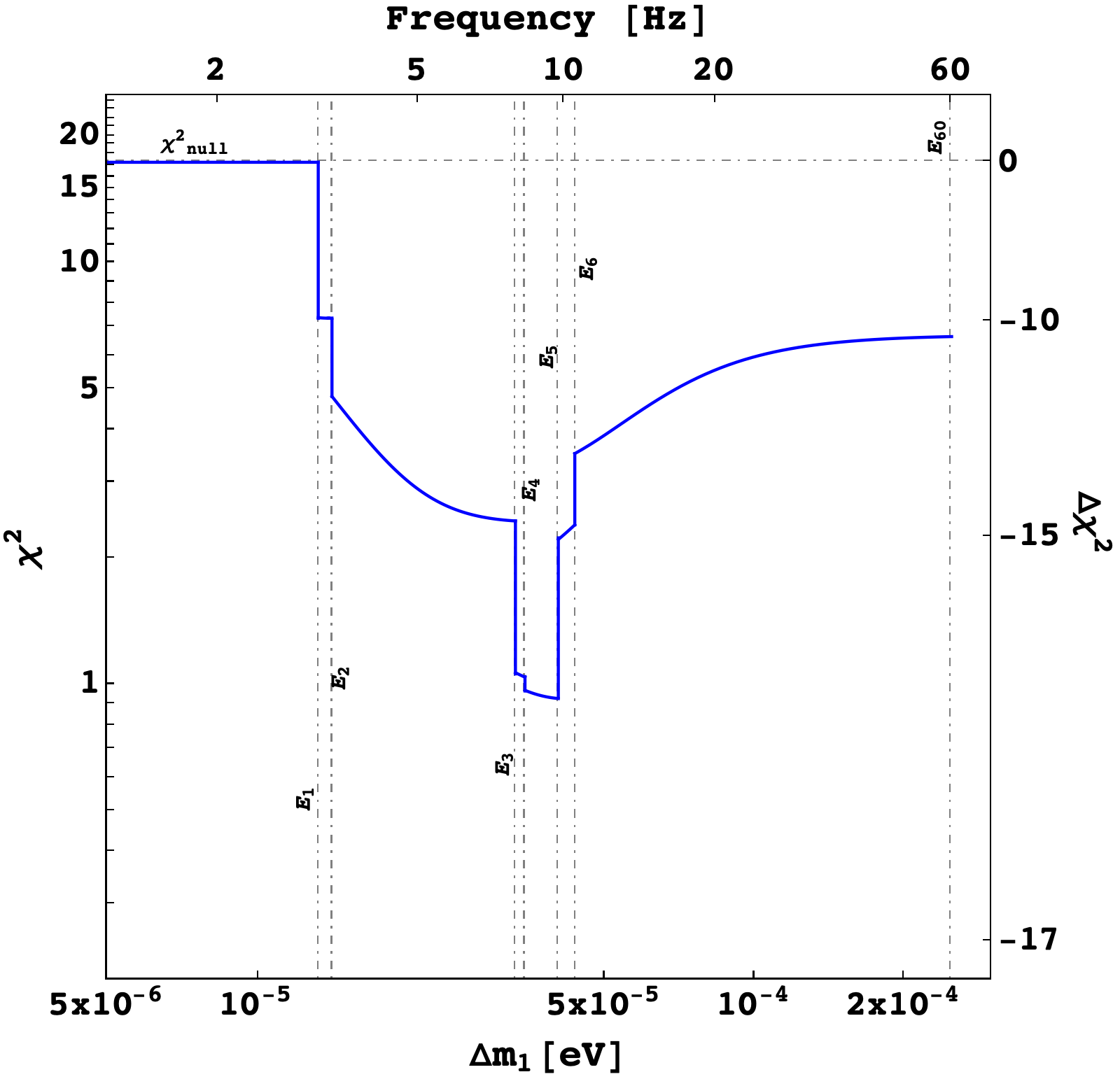
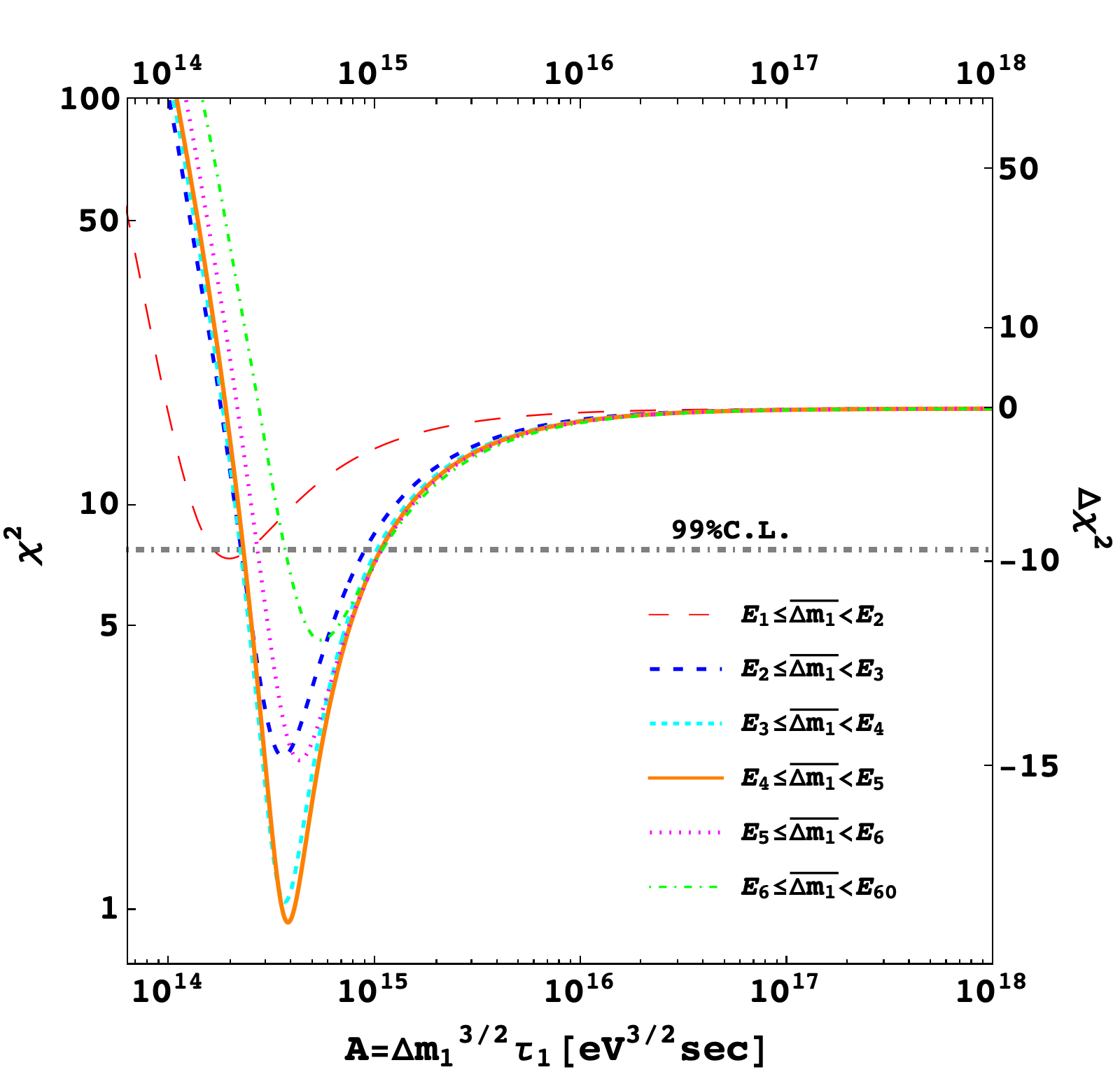
Figure 1: Left panel: $\chi^{2}$ versus $\Delta m_{1}$ for best fit value of $A$ in each interval as in Table 2. Right panel: $\chi^{2}$ as a function of $A$ for the best fit values of $\Delta m_{1}$ in each interval $E_{i}\leq\Delta m_{1}<E_{i+1}$ as in Table 2.

One can clearly notice the jumps at each value $E_{i}$. For $\Delta m_{1}<E_{1}$, one recovers the value $\chi^{2}_{\rm null}=17.2$ (4 d.o.f.) corresponding to the standard case, since there is no observable quantity that can distinguish between the two cases.

Table 2: Results of the fit of ARCADE 2 data. Best fit values, $\chi^{2}$ and $\Delta\chi^{2}$ are shown for each interval of $\Delta m_{1}$, corresponding to a frequency interval between two data points.

Interval	$\overline{A}({\rm eV}^{3\over 2}\,{\rm s})$	$\overline{\Delta m}_{1}$ (eV)	$\overline{\tau}_{1}$ (${\rm s}$)	$\chi^{2}_{{\rm min}}$	$\Delta\chi^{2}_{{\rm min}}$
$E_{1}\leq\Delta m_{1}<E_{2}$	$1.9\times 10^{14}$	$1.4\times 10^{-5}$	$3.6\times 10^{21}$	7.36	-9.87
$E_{2}\leq\Delta m_{1}<E_{3}$	$2.3\times 10^{14}$	$2.7\times 10^{-5}$	$1.6\times 10^{21}$	2.28	-14.95
$E_{3}\leq\Delta m_{1}<E_{4}$	$3.6\times 10^{14}$	$3.4\times 10^{-5}$	$1.8\times 10^{21}$	1.06	-16.17
$E_{4}\leq\Delta m_{1}<E_{5}$	$3.8\times 10^{14}$	$4.0\times 10^{-5}$	$1.46\times 10^{21}$	0.96	-16.27
$E_{5}\leq\Delta m_{1}<E_{6}$	$4.2\times 10^{14}$	$4.3\times 10^{-5}$	$1.49\times 10^{21}$	2.19	-15.04
$E_{6}\leq\Delta m_{1}<E_{60}$	$4.7\times 10^{14}$	$2.0\times 10^{-4}$	$1.66\times 10^{20}$	3.23	-14.00

The results of the fit are shown in Table 2 for each interval: we show best fit values for $A$, $\Delta m_{1}$ and $\tau_{1}$ and corresponding $\chi^{2}_{{\rm min}}$.

In the right panel of Fig. 1 we show the $\chi^{2}$ as a function of $A$ for best fit value of $\Delta m_{1}$ in each interval as indicated. For sufficiently large values of $A$ (i.e., large values of $\tau$), one again always recovers the standard case with $\chi^{2}_{\rm null}=17.2$ (4 d.o.f.). In Table 2 we also show the different values $\Delta\chi^{2}_{{\rm min},i}=\chi^{2}_{{\rm min},i}-\chi^{2}_{\rm null}$. It is intriguing that that the data points seem to indicate that the presence of an end point falling in the interval $E_{4}<E\sim 4\times 10^{-5}\,{\rm eV}\leq E_{5}$ ($\nu_{4}<\nu\simeq 9.7\,{\rm GHz}<\nu_{5}$) as also confirmed by the results of the fit: the best fit is found indeed for $E_{4}<\Delta m_{1}\lesssim E_{5}=4.02\times 10^{-5}\,{\rm eV}$ with $\chi^{2}_{{\rm min},4}=0.96$. In the right panel of Fig. 2 we show the best fit curves for $T_{\gamma_{\rm nth}}(E,0)$ for each interval together with the six ARCADE 2 data points. The thick solid (orange) curve corresponds to the global best fit and it should be clear how well it fits all data points.

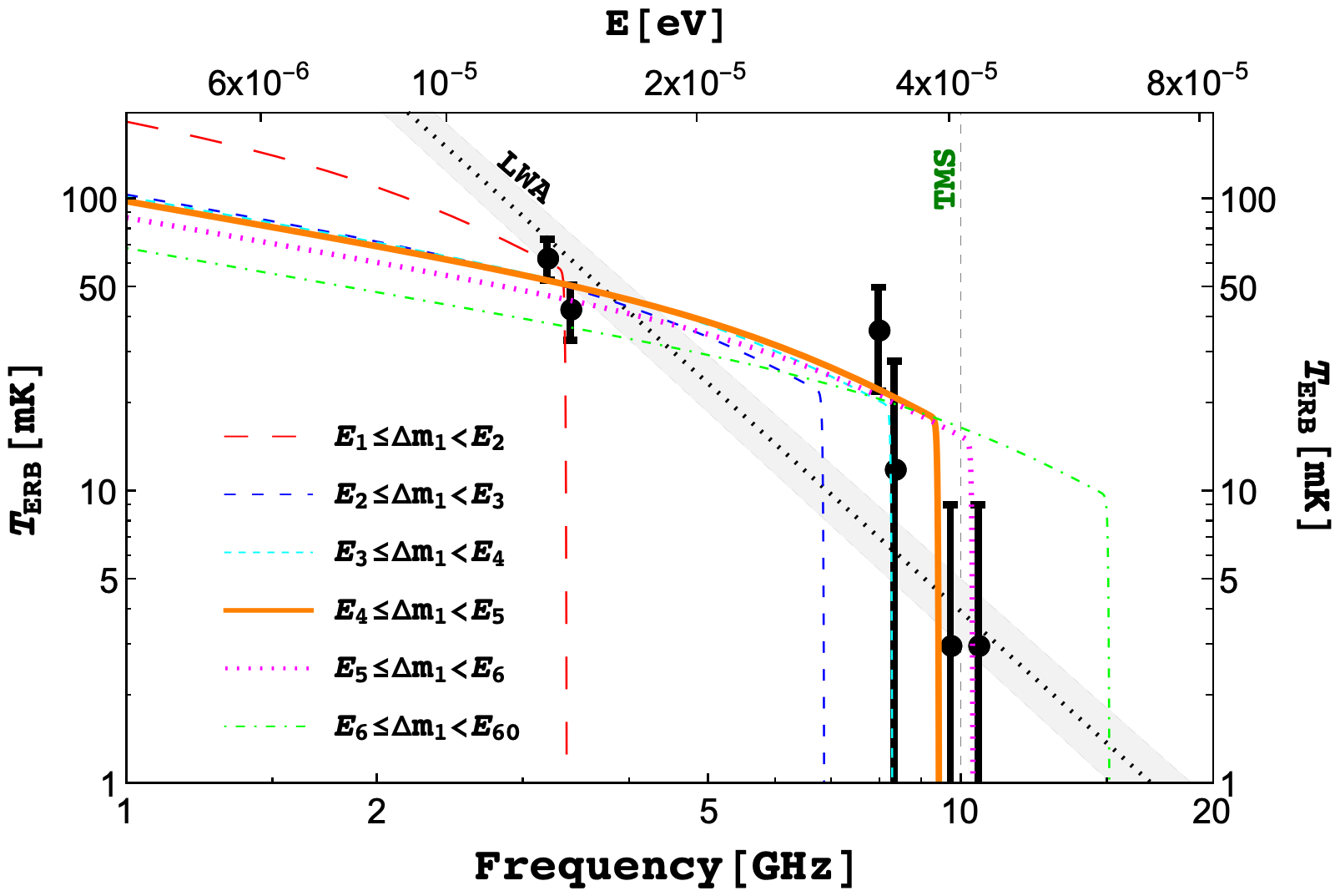
Figure 2: Best fit curves for $T_{\gamma_{\rm nth}}(E,0)$. The thick solid orange curve corresponds to a solution very close to the best global fit ($\Delta m_{1}=4.0\times 10^{-5}\,{\rm eV}$ and $\tau_{1}=1.46\times 10^{21}\,{\rm s}$).

In Fig. 3 we show the resulting $99\%{\rm C.L.}$ allowed region in the plane $\Delta m_{1}$ versus $\tau_{1}$. The different blue shades are indicative of the goodness of the fit. The orange star denotes the global best fit.

If we focus on the interval $E_{4}\leq\Delta m_{1}<E_{5}$, where the best fit is found, we find $\overline{A}\simeq 3.8\times 10^{14}\,{\rm eV}^{3/2}\,{\rm s}$ with $\chi^{2}_{\rm min}/{\rm d.o.f.}\simeq 0.96$ (4 d.of.). For $\chi^{2}\lesssim\chi^{2}_{\rm min}+(2.6)^{2}$, (corresponding approximately to the $99\%\,{\rm C.L.}$ range), we find

$$A=3.8^{+7.2}_{-1.5}\times 10^{14}\,{\rm eV}^{3/2}\,{\rm s}\,.$$ (3.4)

If one interprets the ARCADE 2 excess as due to some alternative explanation than relic neutrino decays, then (3.4) places the $99\%$ C.L. lower bound

$$(\Delta m_{1})^{3/2}\,\tau_{1}>2.3(1.3)\times 10^{14}\,{\rm eV}^{3/2}\,{\rm s}\,,$$ (3.5)

that, as one can see from the figure, approximately holds in the range $2.5\times 10^{-5}\,{\rm eV}<\Delta m_{1}<E_{60}=2.5\times 10^{-4}\,{\rm eV}$ ($E_{1}=1.36\times 10^{-5}\,{\rm eV}\leq\Delta m_{1}\leq 2.5\times 10^{-5}\,{\rm eV}$).

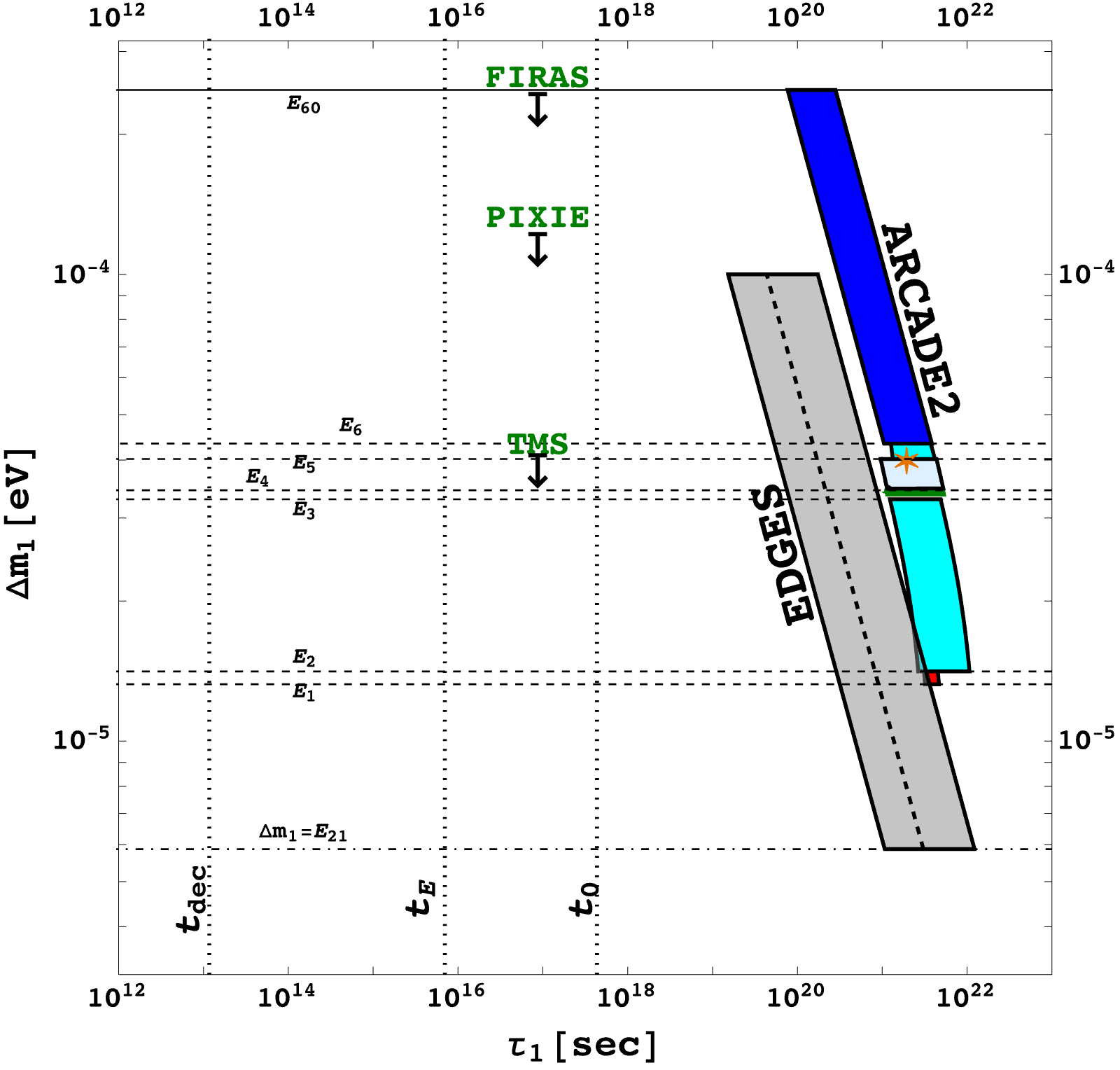
Figure 3: Allowed region in the plane $\Delta m_{1}$ versus $\tau_{1}$ ($99\%$ C.L.). The orange star indicate the best fit found. Colour code: light grey for $\chi^{2}<1$, green for $1<\chi^{2}<2$, cyan for $2<\chi^{2}<3$, blue for $3<\chi^{2}<7$ and red for $7<\chi^{2}<9$.

The ARCADE 2 data can also be combined with additional data also providing evidence for an excess radio background at lower frequencies ($40\,{\rm MHz}\lesssim\nu\lesssim 1.42\,{\rm GHz}$ and in this case a power law yields a very good combined fit [1]. More recently, the Long Wavelength Array (LWA) measured the diffuse radio background between 40 and 80 MHz, also finding an excess. In combination with the data from ARCADE 2 and other experiments, the LWA collaboration finds as best fit the following power law spectrum [3]

$$T_{\rm ERB}=(30.4\pm 2.6)\,\left({\nu\over 310\,{\rm MHz}}\right)^{-2.58\pm 0.05}\,{\rm K}\,.$$ (3.6)

This is shown in Fig. 2 with a grey band. It can be seen however, that especially the third point from ARCADE 2 seems not to be well fit by this power law. One indeed finds $\chi^{2}\simeq 2.5$ (4 d.o.f.), showing that the power law in Eq. (3.6) gives a worse fit to the ARCADE 2 data than the best fit we found but it is still acceptable. However, the power law in Eq. (3.6) still requires some physical source that produces it. It is then legitimate to wonder whether it is possible to combine the success of relic neutrino decays in reproducing the ARCADE 2 data with the success of the power law (3.6) in reproducing data below 1 GHz. As recently pointed out in [19], the account of soft photon heating from free-free processes might provide a plausible solution to find such a combined description of ARCADE 2 with sub-GHz data. In this case the power law would hold up to $\nu\sim 1\,{\rm GHz}$ but should turn into Eq. (3.3) at higher frequencies. Testing such a hypothesis of course would require a new experiment able to collect data points in the 1 GHz–20 GHz range. The TMS experiment will only take data above 10 GHz. This will be certainly still useful to strengthen the hint for the existence of an endpoint and possibly rule out the validity of the power law in Eq. (3.6) up to such high frequencies. However, it will not provide a thorough test of the best fit solution we found to the excess radio background. This could come from a new balloon experiment, an improved version of ARCADE 2. Of course an accurate and precise agreement with the prediction Eq. (3.3) could provide a strong evidence. However, a smoking gun able to test in addition that non-thermal photons were also produced at higher redshifts can be provided by the observation of the 21 cm cosmological global absorption signal.

4 Predicting the 21 cm cosmological global absorption signal

The 21 cm hyperfine transition of the hydrogen atom can be used to test the physics of the cosmic dawn, when first astrophysical sources start to form. It is a transition between the two levels of the 1s ground state of the hydrogen atom. The energy gap, giving the energy of the absorbed or emitted photons at rest in the transition, is $E_{21}=5.87\,\mu{\rm eV}$ corresponding to a 21 cm line rest frequency $\nu_{21}^{\rm rest}=1420\,{\rm MHz}$. The ratio of the population of the excited state, $n_{1}$, to that one of the ground state, $n_{0}$, can be parameterised in terms of a spin temperature $T_{\rm S}(z)$ depending on the redshift:

$${n_{1}\over n_{0}}(z)\equiv{g_{1}\over g_{0}}\,e^{-{E_{21}\over T_{\rm S}(z)}}\,,$$ (4.1)

where $g_{1}/g_{0}=3$ is the excited state-to-ground state degeneracy ratio. The possibility to detect an observable signal from the 21cm cosmological transitions of the hydrogen atoms in the primordial gas after recombination relies on a non-vanishing brightness constrast between the cosmic radiation and the radiation emitted in the 21 cm transitions. This can be parameterised in terms of the 21cm brightness temperature $T_{21}(z)$ [40]

$$T_{21}(z)\simeq 23\,{\rm mK}\,(1+\delta_{B})\,x_{H_{I}}(z)\,\left({\Omega_{{\rm B}0}h^{2}\over 0.02}\right)\,\left[\left({0.15\over\Omega_{{\rm M}0}h^{2}}\right)\,\left({1+z\over 10}\right)\right]^{1/2}\,\left[1-{T_{\gamma}(z)\over T_{S}(z)}\right]\,,$$ (4.2)

where $\delta_{B}=(\rho_{\rm B}-\bar{\rho}_{\rm B})/\bar{\rho}_{\rm B}$ is the fractional baryon overdensity and $x_{H_{I}}(z)$ is the neutral hydrogen fraction. If the spin temperature is equal to the photon temperature ($T_{\rm S}=T_{\gamma}$), then photons are absorbed and reemitted with the same intensity and there is no visible signal. Also, if all atoms are ionised so that $x_{H_{I}}=0$, there cannot be any signal. Another important point to consider is that the spin temperature is related to $T_{\rm gas}$, the kinetic temperature of the gas, by

$$\left(1-{T_{\gamma}\over T_{S}}\right)\simeq{x_{c}+x_{\alpha}\over 1+x_{c}+x_{\alpha}}\,\left(1-{T_{\gamma}\over T_{\rm gas}}\right)\,,$$ (4.3)

where $x_{\alpha}$ and $x_{c}$ are coefficients describing the coupling between the hyperfine levels and the gas. In the limit of strong coupling, for $x_{\alpha}+x_{c}\gg 1$, one has $T_{S}=T_{\rm gas}$, while in the limit of no coupling, for $x_{\alpha}=x_{c}=0$, one has $T_{S}=T_{\gamma}$ and in this case also there is no signal.

From these considerations, one can then draw the following evolution for the 21cm global signal [18, 41].

• The hydrogen gas decouples completely from the cosmic radiation, so that one can have $T_{\rm S}\neq T_{\gamma}$, at a redshift $z_{\rm dec}\simeq 150$. For lower redshifts, the gas cools down more rapidly than cosmic radiation, with $T_{\rm gas}(z)=T(z_{\rm dec})\,(1+z_{\rm dec})^{2}$. Moreover in the redshift range $z_{\rm dec}\gtrsim z\gtrsim 30$, the gas collision rate is high enough that the 21 cm transitions are coupled to the gas temperature and approximately $T_{\rm S}\simeq T_{\rm gas}$. During this stage an absorption signal, for $T_{21}<0$, is expected.

• At redshifts $z\simeq 30$, the gas becomes so rarified that collisions are unable to couple the spin temperature to the gas temperature and one has $x_{a}+x_{c}\ll 1$ and $T_{S}\simeq T_{\gamma}$. Therefore, at this stage $T_{21}\simeq 0$ and there is no 21 cm signal again.

• At redshifts $z_{\star}\simeq 30$, first luminous sources also start to form and this, via Wouthuysen-Field effect, triggers a gradual recoupling of the 21 cm transitions with the gas so that the spin temperature gradually tends again to the gas temperature. In this stage one can again expect an absorption signal since $T_{21}<0$.

• Finally, for redshifts around $z\simeq 10$, the gas gets reheated by the astrophysical radiation and the gas temperature increases. In this stage it might even be possible to have $T_{\rm S}\simeq T_{\rm gas}>T_{\gamma}$, so that one has an emission signal from regions where the gas is not fully ionised. All gas gets eventually ionised, so that the signal switches off again.

The EDGES collaboration has found an absorption profile in the range $z=15$–$20$, with the minimum at a frequency $\nu_{21}(z_{E})\simeq 78\,{\rm MHz}$ corresponding to $z_{E}\simeq 17$ [20]. The absorption profile has a U shape with quite a flat minimum. We do not attempt at fitting the precise shape of the profile since this may be sensitive to systematic errors and the assumed form of the fitted model. However, we will take into account that the exact frequency of the minimum and, consequently, its redshift has an uncertainty and one can actually write $z_{E}=\bar{z}_{E}\pm 1$. Let us first focus on the central value $\bar{z}_{E}=17$. At this value, the $\Lambda$CDM model predicts a relic photon temperature

$$T_{\gamma}(\bar{z}_{E})=T(\bar{z}_{E})=T_{0}\,(1+\bar{z}_{E})\simeq 49.6\,{\rm K}\,$$ (4.4)

and a gas temperature $T_{\rm gas}(\bar{z}_{E})\simeq 7.2\,{\rm K}$. Defining $\xi(z)\equiv T_{\gamma}(z)/T_{\rm gas}(z)$, one has then $\xi(\bar{z}_{E})\simeq 6.89$, corresponding, to $T_{21}(\bar{z}_{E})\simeq-206\,{\rm mK}$ from Eq. (4.2).

On the other hand, the EDGES collaboration finds a much stronger absorption signal with $T_{21}^{\rm EDGES}(z_{E})=-500^{+200}_{-500}\,{\rm mK}$ ($99\%\,{\rm C.L.}$). From Eq. (4.2), this translates into

$$\xi^{\rm EDGES}(\bar{z}_{E})=15.1_{-5.6}^{+14.1}\,,$$ (4.6)

and from this one finds first

$$T^{\rm EDGES}_{\gamma}(\bar{z}_{E})=\xi^{\rm EDGES}(\bar{z}_{E})\,T_{\rm gas}(\bar{z}_{E})=109^{+101}_{-41}\,{\rm K}\,,$$ (4.7)

and then finally, subtracting the temperature of thermal photons, one obtains for the effective temperature of the non-thermal contribution ($99\%\,{\rm C.L.}$)

$$T^{\rm EDGES}_{\gamma_{\rm nth}}(\bar{z}_{E})=(60^{+101}_{-41})\,{\rm K}\,.$$ (4.8)

Finally, we have also calculated the additional error coming from the uncertainty $\Delta z_{E}=\pm 1$ and found that this is of order of $3\,{\rm K}$ so that, once added in quadrature, it gives a negligible increase of $0.1\,{\rm K}$ to the total error.

This is the experimental quantity we need to reproduce. We have now to use Eq. (2.6) to calculate the effective temperature from the specific intensity and Eq. (2.1) for the specific intensity of photons produced from relic neutrino decays. This time, in the case of EDGES, the redshift is $z_{E}$ and the energy is $E_{21}$, so that we obtain

$$T_{\gamma_{\rm nth}}(E_{21},z_{E})\simeq{6\,\zeta(3)\over 11\,\sqrt{\Omega_{{\rm M}0}}}\,{T_{0}^{3}\,(1+z_{E})^{3/2}\over E_{21}^{1/2}\,\Delta m_{1}^{3/2}}\,{t_{0}\over\tau_{1}}\,,$$ (4.9)

where notice we have used $H(z_{E})=H_{0}\,\sqrt{\Omega_{M0}}\,(1+z_{E})^{3/2}$. Imposing that this predicted effective temperature reproduces the experimental measurement in Eq. (4.8), one finds ($99\%\,{\rm C.L.}$)

$$A^{\rm EDGES}(\bar{z}_{E})={6\,\zeta(3)\over 11\,\sqrt{\Omega_{{\rm M}0}}}\,{T_{0}^{3}\,(1+\bar{z}_{E})^{3/2}\over T^{\rm EDGES}_{\gamma_{\rm nth}}(\bar{z}_{E})\,E_{21}^{1/2}}\,t_{0}=(4.0^{+8.8}_{-2.5})\times 10^{13}\,.$$ (4.10)

This result holds in the range $E_{21}=5.87\,\mu{\rm eV}\leq\Delta m_{1}\lesssim 10^{-4}\,{\rm eV}$. The lower bound is clear since only photons produced with energies above $E_{21}$ at redshifts $z_{\rm D}\geq z_{E}$ can excite the Hydrogen atoms ground states. The upper bound is due to the fact that we are treating neutrinos as non-relativistic at decays. Therefore, one has to impose $T_{\nu}(z_{\rm D})\lesssim 0.5\,m_{1}\lesssim 0.05\,{\rm eV}$. This implies $1+z_{\rm D}\lesssim 300$ and consequently $\Delta m_{1}\lesssim E_{21}(1+z_{\rm D})/(1+z_{E})\sim 10^{-4}\,{\rm eV}$.

The resulting ($99\%\,{\rm C.L.}$) allowed region in the plane $\Delta m_{1}$ versus $\tau_{1}$ is shown in Fig. 3 in light grey. This has be compared with the allowed region obtained fitting ARCADE 2 data in Eq. (3.4). It is clear that the two regions only marginally overlap and so there is some tension between the two results. This tension might be reconciled if the current EDGES measurement is overestimating the 21 cm global absorption signal.

Reversely, it is easy to derive a prediction for the contrast brightness temperature $T_{21}$, that future 21 cm cosmology experiments should measure, starting from our ARCADE 2 data fit. This can be simply done plugging first Eq. (3.4), giving the ($99\%\,{\rm C.L.}$) allowed range for $A$ from ARCADE 2 data at the best fit value for $\Delta m_{1}$, into Eq. (4.9), finding $T_{\gamma_{\rm nth}}(E_{21},z_{E})$, and then from Eq. (4.2) one obtains ($99\%$ C.L.):

$$T_{21}(\bar{z}_{E})=-238^{+21}_{-20}\,{\rm mK}\,.$$ (4.11)

When this is compared with the EDGES measurement, unsurprisingly, one again finds the same kind of tension found in terms of $A$, now expressed in terms of the observable $T_{21}$. The result (4.11) is one of our main results, since it is another clear prediction of the model. This together with a test of the predictions of the excess radio background effective temperature, represents a clear signature of the model.

5 On dark matter decays/de-excitations as alternative explanation

The solution we have found can also be mimicked by replacing relic neutrino decays with dark matter decays or de-excitations. For example, we can have in mind a picture where dark matter is made of some dark atoms and photons are produced from de-excitations of the first excited state into the ground state. Indicating with $m_{\rm DM}$ the mass of dark matter and with $f_{\rm D}$ the fraction of dark matter abundance in the excited state, then we obtain for the effective temperature of the excess radio background

$$T^{(\rm DM)}_{\gamma_{\rm nth}}(E,0)={\pi^{2}\,f_{\rm D}\,n^{\infty}_{\rm DM}(0)\over E^{2}}\,{e^{-{t(a_{\rm D})\over\tau_{\rm DM}}}\over H(a_{\rm D})\,\tau_{\rm DM}}\,.$$ (5.1)

The (average) dark matter number density at the present time is simply given by

$$n^{\infty}_{\rm DM}(0)={\rho_{{\rm c}0}h^{-2}\over m_{\rm DM}}\,\Omega_{{\rm DM}0}h^{2}\simeq 1.265\,{{\rm GeV}\over m_{\rm DM}}\,{\rm m}^{-3}\,,$$ (5.2)

where we used $\Omega_{\rm DM}h^{2}=0.11933$ [39] and $\rho_{{\rm c}0}h^{-2}=10.54\,{\rm GeV}\,{\rm m}^{-3}$. In terms of the neutrino number density $n_{\nu_{1}}^{\infty}(0)$ (see Eq. (2.2)), it can also be rewritten as

$$n^{\infty}_{\rm DM}(0)={11.3\,{\rm eV}\over m_{\rm DM}}\,n_{\nu_{1}}^{\infty}(0)\,.$$ (5.3)

In this way the effective temperature of the excess radio background for dark matter de-excitations can be expressed in terms of the one we found for relic neutrino decays (Eq. (3.3)):

$$T^{(\rm DM)}_{\gamma_{\rm nth}}(E,0)=\left({11\,{\rm eV}\,f_{\rm D}\over m_{\rm DM}}\right)\,{{\tau}_{1}\over\tau_{\rm DM}}\,T^{(\nu)}_{\gamma_{\rm nth}}(E,0)\,e^{-{t(a_{\rm D})\over\tau_{\rm DM}}}\,.$$ (5.4)

If we approximate $t(a_{\rm D})\simeq t_{0}$, strictly valid for $E=\Delta m_{1}$, then it is clear that the same solution we obtained for neutrinos is also obtained for dark matter decays/deexcitations replacing $\tau_{1}\rightarrow\tau_{\rm DM}$ (and of course $\Delta m_{1}\rightarrow\Delta m_{\rm DM}$) for

$$m_{\rm DM}\,f^{-1}_{\rm D}\sim 10\,{\rm keV}{t_{0}\over\tau_{\rm DM}}\,e^{-{t_{0}\over\tau_{\rm DM}}}\,.$$ (5.5)

As far as $\tau_{\rm DM}\ll t_{0}$, one can see that for $m_{\rm DM}/f_{\rm D}\sim 10\,{\rm eV}$, one obtains the same value for the lifetime we obtained for neutrinos, $\tau_{\rm DM}\sim\bar{\tau}_{1}\sim 10^{21}\,{\rm s}$. For higher values of $m_{\rm DM}$, the lifetime, and therefore the value of $A$, decreases as $\tau_{\rm DM}\propto(m_{\rm DM}/f_{\rm D})^{-1}$. When $\tau_{\rm DM}\lesssim t_{0}$, for $m_{\rm DM}/f_{\rm D}\sim 10\,{\rm keV}$, the exponential kicks in and the effective temperature start to be suppressed exponentially and the ARCADE 2 data cannot be reproduced for larger values so that one obtains the upper bound

$$m_{\rm DM}\lesssim 10\,{\rm keV}\,f_{\rm D}\,.$$ (5.6)

Notice though that one can still reproduce the EDGES data since in that case one has to replace $t_{0}\rightarrow t_{E}=t(\bar{z}_{E})\simeq 250\,{\rm Myr}\sim 10^{16}\,{\rm s}$. In this case the upper bound relaxes by about two orders of magnitude. Of course in this case it would be impossible to reconcile the EDGES anomaly and ARCADE 2 excess radio background.

We should also make clear that this upper bound on the dark matter mass is obtained under the assumptions of validity of the solution. In particular, this assumes that the excess radio background is explained by the primary photons produced from dark matter decays/deexcitations that are simply redshifted from decays to the present time in case of the excess radio background or to $t_{E}$ in the case of the EDGES anomaly. This does not exclude that other processes, such as soft photon heating, could be active at higher dark matter mass or mass difference values, reprocessing injected photons and reproducing the excess radio background though with a different spectrum, typically a power law one [19].

Finally, notice that these strong limitations on a solution in terms of dark matter decays/de-excitations are in addition to the strong constraints from the smoothness of the excess radio background that clashes with the expected anisotropies of the signal that should track the dark matter distribution.

6 Final remarks

Let us conclude with some final remarks on the solution to the excess radio background we have discussed.

• We have referred to the case of lightest neutrino decays into sterile neutrinos. However, as we said in the introduction, the discussion is equally applicable to the case when of the the two heavier light neutrinos, either $\nu_{2}$ or $\nu_{3}$, decay into sterile neutrinos, simply one has to replace everywhere $\Delta m_{1},\tau_{1}\rightarrow\Delta m_{2,3},\tau_{2,3}$. The difference is that $m_{2}$ and $m_{3}$ are lower bounded by the solar neutrino and atmospheric neutrino mass scale, respectively, explicitly $m_{2}\gtrsim 8\,{\rm meV}$ and $m_{3}\gtrsim 50\,{\rm meV}$ (in this case $m_{1}$ can be arbitrarily small). This lower bound guarantees they are automatically non-relativistic in all the relevant range of redshifts ($0$–$300$). On the other hand, in the case of lightest active neutrinos, we have to impose $m_{1}\gtrsim 10\,{\rm meV}$, an interesting condition that will be tested during next years by absolute neutrino mass scale experiments.

• The solution we found predicts an effective temperature of the excess radio background that depends as $\propto E^{-0.5}$ for $a_{\rm D}=E/\Delta m_{i}\lesssim a_{\rm eq}\simeq 0.75$ and as $\propto E^{-1.5}$ for $a_{\rm D}\gtrsim 0.75$ and an abrupt endpoint at $E=\Delta m_{i}$. These are all features that makes it distinguishable from other solutions and in particular from the power law Eq. (3.6). To this extent measurements in the frequency range $\nu=1\,{\rm}$–$20\,{\rm GHz}$ would be needed and so an improved ARCADE 2-like experiment would be certainly a priority . The TMS microwave telescope, will only partly test the solution at $\nu\geq 10\,{\rm GHz}$. The best fit solution we found predicts no excess will be detected at TMS. On the other hand, one expects that the power law, well describing the excess radio background measurements at low frequencies, should be recovered accounting for processes such as soft photon heating reprocessing lower frequency photons.

• As pointed out in [12], there is a second solution for life-times much shorter than the age of the universe. In this case the exponential in Eq. (3.3) cannot be neglected. However, this solution is strongly fine-tuned and it is lives only for a very narrow range of $A$ values. In addition, for such short life-times, free-free processes should be taken into account. Moreover, this solution predicts a negligible deviation in the absorption 21 cm cosmological signal from the standard case, so that the tension with the EDGES anomaly is even more exacerbated.

• The excess radio background is a detection of photons produced by relic neutrino decays at relatively low redshifts (the highest redshift for the best fit solution is given by $z\simeq E_{5}/E_{1}-1\simeq 2$). However, the 21 cm global signal is sensitive also to photons produced at higher redshifts (up to $\sim 300$). In particular, we have seen how solution for the excess radio background predicts $T_{21}\simeq-240\,{\rm mK}$. This is another very specific prediction that will be tested during next years. This prediction is in mild tension with the anomalous EDGES measurement. A possible explanation is that this might have been overestimated due to some unidentified foreground.

• The same solution we found in the case of relic neutrino decays could also be mimicked by decays/de-excitations of some fraction $f_{\rm D}$ of (cold) dark matter. However, this solution is only possible for masses $m_{\rm DM}/f_{\rm D}\lesssim 10\,{\rm keV}$. This limitation is in addition to the difficulty of such solutions to explain the smoothness of the excess radio background, since they unavoidably predict anisotropies tracking the dark matter distribution.

• The solution we have presented can be nicely realised within a model where neutrinos are unstable, this will be presented in a forthcoming paper [43].

It is quite exciting that radio background experiments have the opportunity during next years to test the stability of the cosmic neutrino background. The relic neutrino decay solution of the excess radio background we have discussed clearly relies on new physics and, therefore, it might provide a very important guidance toward an extension of our current established fundamental theories of nature.

Acknowledgments

The work of BD was partly supported by the U.S. Department of Energy under grant No. DE- SC 0017987. PDB and RR acknowledge financial support from the STFC Consolidated Grant ST/T000775/1. IMS is supported by STFC grant ST/T001011/1. This project has received funding from the European Union’s Horizon Europe research and innovation programme under the Marie Skłodowska-Curie Staff Exchange grant agreement No. 101086085 – ASYMMETRY. In particular, PDB wishes to thank the MIT Center for Theoretical Physics for the hospitality and Tracy Slatyer for useful discussions.

References

- [1] D.J. Fixsen et al., ARCADE 2 Measurement of the Extra-Galactic Sky Temperature at 3-90 GHz, Astrophys. J. 734 (2011) 5 [0901.0555].
- [2] D.J. Fixsen and J.C. Mather, The Spectral Results of the Far-Infrared Absolute Spectrophotometer Instrument on COBE, Astrophys. J. 581 (2002) 817.
- [3] J. Dowell and G.B. Taylor, The Radio Background Below 100 MHz, Astrophys. J. Lett. 858 (2018) L9 [1804.08581].
- [4] J. Singal et al., The Radio Synchrotron Background: Conference Summary and Report, Publ. Astron. Soc. Pac. 130 (2018) 036001 [1711.09979].
- [5] N. Fornengo, R.A. Lineros, M. Regis and M. Taoso, The isotropic radio background revisited, JCAP 04 (2014) 008 [1402.2218].
- [6] T. Vernstrom, R.P. Norris, D. Scott and J.V. Wall, The Deep Diffuse Extragalactic Radio Sky at 1.75 GHz, Mon. Not. Roy. Astron. Soc. 447 (2015) 2243 [1408.4160].
- [7] G.P. Holder, The unusual smoothness of the extragalactic unresolved radio background, Astrophys. J. 780 (2014) 112 [1207.0856].
- [8] N. Fornengo, R. Lineros, M. Regis and M. Taoso, Possibility of a Dark Matter Interpretation for the Excess in Isotropic Radio Emission Reported by ARCADE, Phys. Rev. Lett. 107 (2011) 271302 [1108.0569].
- [9] A. Caputo, H. Liu, S. Mishra-Sharma, M. Pospelov and J.T. Ruderman, Radio excess from stimulated dark matter decay, Phys. Rev. D 107 (2023) 123033 [2206.07713].
- [10] R. Brandenberger, B. Cyr and R. Shi, Constraints on Superconducting Cosmic Strings from the Global -cm Signal before Reionization, JCAP 09 (2019) 009 [1902.08282].
- [11] S. Mittal and G. Kulkarni, Background of radio photons from primordial black holes, Mon. Not. Roy. Astron. Soc. 510 (2022) 4992 [2110.11975].
- [12] M. Chianese, P. Di Bari, K. Farrag and R. Samanta, Probing relic neutrino radiative decays with 21 cm cosmology, Phys. Lett. B 790 (2019) 64 [1805.11717].
- [13] S.K. Acharya, J. Dhandha and J. Chluba, Can accreting primordial black holes explain the excess radio background?, Mon. Not. Roy. Astron. Soc. 517 (2022) 2454 [2208.03816].
- [14] S.K. Acharya and J. Chluba, A closer look at dark photon explanations of the excess radio background, Mon. Not. Roy. Astron. Soc. 521 (2023) 3939 [2209.09063].
- [15] A. Kogut et al., The Primordial Inflation Explorer (PIXIE): A Nulling Polarimeter for Cosmic Microwave Background Observations, JCAP 07 (2011) 025 [1105.2044].
- [16] P. Alonso-Arias, P.A. Fuerte-Rodríguez, R.J. Hoyland and J.A. Rubiño Martín, The optical system of the Tenerife Microwave Spectrometer: a window for observing the 10–20 GHz sky spectra, JINST 16 (2021) P12037.
- [17] C. Feng and G. Holder, Enhanced global signal of neutral hydrogen due to excess radiation at cosmic dawn, Astrophys. J. Lett. 858 (2018) L17 [1802.07432].
- [18] S. Furlanetto, S.P. Oh and F. Briggs, Cosmology at Low Frequencies: The 21 cm Transition and the High-Redshift Universe, Phys. Rept. 433 (2006) 181 [astro-ph/0608032].
- [19] S.K. Acharya, B. Cyr and J. Chluba, The role of soft photon injection and heating in 21 cm cosmology, Mon. Not. Roy. Astron. Soc. 523 (2023) 1908 [2303.17311].
- [20] J.D. Bowman, A.E.E. Rogers, R.A. Monsalve, T.J. Mozdzen and N. Mahesh, An absorption profile centred at 78 megahertz in the sky-averaged spectrum, Nature 555 (2018) 67 [1810.05912].
- [21] R. Hills, G. Kulkarni, P.D. Meerburg and E. Puchwein, Concerns about modelling of the EDGES data, Nature 564 (2018) E32 [1805.01421].
- [22] R.F. Bradley, K. Tauscher, D. Rapetti and J.O. Burns, A Ground Plane Artifact that Induces an Absorption Profile in Averaged Spectra from Global 21-cm Measurements - with Possible Application to EDGES, Astrophys. J. 874 (2019) 153 [1810.09015].
- [23] S. Singh, J. Nambissan T., R. Subrahmanyan, N. Udaya Shankar, B.S. Girish, A. Raghunathan et al., On the detection of a cosmic dawn signal in the radio background, Nature Astron. 6 (2022) 607 [2112.06778].
- [24] R.A.M.R.e.a. Bowman, J.D., Reply to Hills et al., Nature Astron. (2018) .
- [25] S.G. Murray, J.D. Bowman, P.H. Sims, N. Mahesh, A.E.E. Rogers, R.A. Monsalve et al., A Bayesian calibration framework for EDGES, Mon. Not. Roy. Astron. Soc. 517 (2022) 2264 [2209.03459].
- [26] H.T.J. Bevins, A. Fialkov, E.d.L. Acedo, W.J. Handley, S. Singh, R. Subrahmanyan et al., Astrophysical constraints from the SARAS 3 non-detection of the cosmic dawn sky-averaged 21-cm signal, Nature Astron. 6 (2022) 1473 [2212.00464].
- [27] G. Bernardi, J.T.L. Zwart, D. Price, L.J. Greenhill, A. Mesinger, J. Dowell et al., Bayesian constraints on the global 21-cm signal from the Cosmic Dawn, Mon. Not. Roy. Astron. Soc. 461 (2016) 2847 [1606.06006].
- [28] J. Singal et al., The Second Radio Synchrotron Background Workshop: Conference Summary and Report, Publ. Astron. Soc. Pac. 135 (2023) 036001 [2211.16547].
- [29] L. Philip, Z. Abdurashidova, H.C. Chiang, N. Ghazi, A. Gumba, H.M. Heilgendorff et al., Probing Radio Intensity at High-Z from Marion: 2017 Instrument, Journal of Astronomical Instrumentation 8 (2019) 1950004 [1806.09531].
- [30] E. de Lera Acedo et al., The REACH radiometer for detecting the 21-cm hydrogen signal from redshift z 7.5–28, Nature Astron. 6 (2022) 998 [2210.07409].
- [31] HERA collaboration, Improved Constraints on the 21 cm EoR Power Spectrum and the X-Ray Heating of the IGM with HERA Phase I Observations, Astrophys. J. 945 (2023) 124 [2210.04912].
- [32] X. Chen, J. Yan, L. Deng, F. Wu, L. Wu, Y. Xu et al., Discovering the Sky at the Longest wavelengths with a lunar orbit array, Phil. Trans. Roy. Soc. Lond. A 379 (2020) 20190566 [2007.15794].
- [33] S.D. Bale, N. Bassett, J.O. Burns, J. Dorigo Jones, K. Goetz, C. Hellum-Bye et al., LuSEE ’Night’: The Lunar Surface Electromagnetics Experiment, arXiv e-prints (2023) arXiv:2301.10345 [2301.10345].
- [34] R. Barkana, Possible interaction between baryons and dark-matter particles revealed by the first stars, Nature 555 (2018) 71 [1803.06698].
- [35] J.B. Muñoz and A. Loeb, A small amount of mini-charged dark matter could cool the baryons in the early Universe, Nature 557 (2018) 684 [1802.10094].
- [36] A. Ewall-Wice, T.C. Chang, J. Lazio, O. Dore, M. Seiffert and R.A. Monsalve, Modeling the Radio Background from the First Black Holes at Cosmic Dawn: Implications for the 21 cm Absorption Amplitude, Astrophys. J. 868 (2018) 63 [1803.01815].
- [37] P. Mertsch, G. Parimbelli, P.F. de Salas, S. Gariazzo, J. Lesgourgues and S. Pastor, Neutrino clustering in the Milky Way and beyond, JCAP 01 (2020) 015 [1910.13388].
- [38] E. Masso and R. Toldra, Photon spectrum produced by the late decay of a cosmic neutrino background, Phys. Rev. D 60 (1999) 083503 [astro-ph/9903397].
- [39] Planck collaboration, Planck 2018 results. VI. Cosmological parameters, Astron. Astrophys. 641 (2020) A6 [1807.06209].
- [40] M. Zaldarriaga, S.R. Furlanetto and L. Hernquist, 21 Centimeter fluctuations from cosmic gas at high redshifts, Astrophys. J. 608 (2004) 622 [astro-ph/0311514].
- [41] J.R. Pritchard and A. Loeb, 21-cm cosmology, Rept. Prog. Phys. 75 (2012) 086901 [1109.6012].
- [42] A. Fialkov and R. Barkana, Signature of Excess Radio Background in the 21-cm Global Signal and Power Spectrum, Mon. Not. Roy. Astron. Soc. 486 (2019) 1763 [1902.02438].
- [43] B. Dev, P. Di Bari, I. Martínez-Soler and R. Rishav.