Universality in driven open quantum matter

Abstract

Universality is a powerful concept, which enables making qualitative and quantitative predictions in systems with extensively many degrees of freedom. It finds realizations in almost all branches of physics, including in the realm of nonequilibrium systems. Our focus here is on its manifestations within a specific class of nonequilibrium stationary states: driven open quantum matter. Progress in this field is fueled by a number of uprising platforms ranging from light-driven quantum materials over synthetic quantum systems like cold atomic gases to the functional devices of the noisy intermediate scale quantum era. These systems share in common that, on the microscopic scale, they obey the laws of quantum mechanics, while detailed balance underlying thermodynamic equilibrium is broken due to the simultaneous presence of Hamiltonian unitary dynamics and nonunitary drive and dissipation. The challenge is then to connect this microscopic physics to macroscopic observables, and to identify universal collective phenomena that uniquely witness the breaking of equilibrium conditions, thus having no equilibrium counterparts. In the framework of a Lindblad-Keldysh field theory, we discuss on the one hand the principles delimiting thermodynamic equilibrium from driven open stationary states, and on the other hand show how unifying concepts such as symmetries, the purity of states, and scaling arguments are implemented. We then present instances of universal behavior structured into three classes: new realizations of paradigmatic nonequilibrium phenomena, including a survey of first experimental realizations; novel instances of nonequilibrium universality found in these systems made of quantum ingredients; and genuinely quantum phenomena out of equilibrium, including in fermionic systems. We also discuss perspectives for future research on driven open quantum matter.

I Introduction

Universality underlies the possibility to perform the transition from micro- to macrophysics quantitatively by systematically discarding irrelevant information. Historically, the concept of universality has guided and enabled progress in many-particle physics in thermodynamic equilibrium. But it is operative more generally in Nature, in systems with an extensive number of degrees of freedom. This work surveys expressions of universality in driven open quantum matter. Systems that belong to this class are defined by the appearance of coherent and driven-dissipative dynamics on an equal footing, placing them far from thermodynamic equilibrium, even if they reach a stationary state.

I.1 Universality

The most dramatic expression of universality occurs close to the critical point of a second order phase transition: There, the loss of memory about the microscopic physics is so strong, that the long-wavelength physics is fully determined by the dimensionality, symmetries and conservation laws, as well as the range of interactions. A system with extensively many degrees of freedom is then characterized by few universal critical exponents defining the universality class. Only a handful of such universality classes are found in Nature, despite the plethora of materials and tailor-made platforms that make up the world around us [237, 642, 286].

Universality, however, manifests in a variety of forms. In its weakest form, universality may be viewed as the fact that Nature is organized hierarchically. Focusing on universality more quantitatively, a suitable starting point is a model of a system which applies on length and time scales that can be considered as microscopic. The goal is then to bridge to the macroscopic physics emerging on scales that are a few (but not many) decades larger. In that setting, universality often results in cases of degeneracies, giving rise to gapless phases of matter that can exist without fine-tuning to a critical point across an extended parameter range. Such situations are characterized by large-scale fluctuations dominating the macroscopic behavior. Mechanisms enabling degeneracies are manifold. One case in point is the spontaneous breakdown of continuous global symmetries, leading to gapless Goldstone modes. Examples include phonons in solids or phase modes in atomic Bose-Einstein condensates. Additionally, soft modes can occur in situations where symmetry breaking is prohibited due to low dimensionality. Universal effects are even enhanced due to the restricted available phase space, as seen in the Kosterlitz-Thouless critical phase in two dimensions. Another class of stable gapless modes appears in the form of hydrodynamics, associated with global conservation laws. Examples include particle and heat diffusion in number and energy-conserving systems, as well as the response of topological insulators.

All the examples mentioned above are consistent with thermodynamic equilibrium conditions, but their fundamental characteristics are not limited to this context. Both criticality and weaker realizations of universal behavior have been established in nonequilibrium statistical mechanics. A paradigmatic example of a nonequilibrium critical point occurs in directed percolation, a variant of the percolation problem that violates detailed balance [520, 251, 248, 115, 297, 284, 451]. Universal nonequilibrium phases facilitated by robust gapless modes are exemplified by the Kardar-Parisi-Zhang equation [316, 343, 269, 561]. It was introduced to describe the roughening of driven interfaces observed in phenomena like the spreading of fire fronts [412] or the growth of bacterial colonies [12]. The phenomenon of self-organized criticality stands in between these cornerstones: A system self-tunes to criticality, and due to this mechanism exhibits stable universal behavior in extended parameter regimes [39, 38, 37, 453, 176, 256, 601, 29, 488]

I.2 Driven Open Quantum Matter

This article focuses on universality in driven open quantum matter, representing a novel class of nonequilibrium many-body systems. The distinguishing feature of systems in this class is the simultaneous presence of coherent quantum dynamics, external drive, and dissipation. This circumstance is typically realized when matter is strongly coupled to external light fields, like lasers. The ability to drive thermodynamically large systems with such fields without compromising their intricate many-body behavior due to noise and heating has emerged relatively recently. Yet it already includes a broad spectrum of platforms for atoms, light, and solids. Among these are exciton-polariton systems in semiconductor heterostructures [120], atoms [425] or solids [291] immersed into cavities, photonic platforms and microcavity arrays [275, 447, 448, 456], circuit quantum electrodynamics [593, 66], ultracold atoms and ions [435, 273], Rydberg gases [83, 509, 429], and light-induced superconductors [424, 122]. Driven open quantum matter also encompasses functionalized matter, such as noisy intermediate-scale quantum (NISQ) [481] devices of superconducting circuits [514] and Rydberg tweezer arrays [533]. The need to conceptualize these systems as instances of driven open quantum matter is clear; this need also starts to get recognized more widely for systems such as cold atoms in optical lattices, specifically when long time scales are being considered [467].

All such systems in the class of driven open quantum matter have two common characteristics:

Nonequilibrium conditions.

The combination of external driving and the coupling to external reservoirs, inducing an open system character, pushes driven open quantum matter out of equilibrium. Without external drive, open systems may still reach thermodynamic equilibrium with their surroundings, and thus obey the principle of detailed balance. The study of such open systems in thermodynamic equilibrium has been pioneered by Caldeira and Leggett [104, 105, 611], building on the influence functional techniques introduced by Feynman and Vernon [197]. However, adding a drive—for example, in the form of a laser field—generically induces stationary fluxes of quantities such as energy, particle number, or entropy, and, therefore, leads to a violation of detailed balance between system and environment. The presence of nonequilibrium conditions even in the stationary state distinguishes driven open systems from closed and undriven many-body systems. Even though the latter can exhibit nonequilibrium behavior in their time evolution, they generically reach a stationary state of thermodynamic equilibrium.

Quantum dynamics.

On the microscopic scale, instances of driven open quantum matter need to be described as quantum systems—quantum mechanical effects such as phase coherence and entanglement cannot be discarded. However, given the delicate nature of quantum mechanical correlations, this does not imply that a quantum mechanical effects necessarily persist up to macroscopic scales. In many instances, an effective (semi-)classical description of the macroscopic behavior is possible—in parallel to finite temperature quantum systems. However, drive and dissipation need not act destructively on quantum many-body correlations, and can even be harnessed to induce them [166, 585]. Identifying and describing universal effects of this type is both a unique challenge and an opportunity offered by driven open quantum systems. This holds the potential to spark a new field of nonequilibrium quantum statistical mechanics.

Realizations of paradigmatic	Novel nonequilibrium universality	Quantum nonequilibrium phenomena
nonequilibrium universality
V. Absorbing state phase transitions	VIII. Driven open criticality	XI. Quantum criticality in driven open systems
and directed percolation
VI. Self-organized criticality and	IX. Slowly and rapidly driven open systems	XII. Universality in dissipative quantum impurities
Rydberg experiments
	X. Nonequilibrium first order phase transitions	XIII. Universality in fermion systems
VII. Driven open condensates in low spatial dimensions

Table 1: Manifestations of universality in driven open quantum matter are grouped into three main directions in this review.

I.3 Synopsis

This review provides both the conceptual framework to characterize universality in driven open quantum matter, and highlights key instances of universality in various physical platforms. It is organized as follows.

Principles of universality in driven open quantum matter (Secs. II–IV).

Microscopically, the systems described above can be modelled in terms of a Markovian quantum master equation in Lindblad form. Yet, this is not the ideal language to distill universality. We thus first introduce an overarching framework that enables discarding irrelevant information while keeping the relevant one (Secs. II–IV). This is achieved by reformulating the quantum master equation in terms of an equivalent but more flexible Lindblad-Keldysh field theory (Sec. II). In particular, this allows us to identify three principles to preserve the relevant information, and to guide the analysis of the driven open quantum many-body problem:

• Equilibrium vs. nonequilibrium stationary states (Sec. III): Detailed balance characteristic of a system in thermodynamic equilibrium is indicated by the presence of a discrete symmetry of the Keldysh action. This equips us with a criterion to distinguish equilibrium from nonequilibrium conditions in practice. By comparing the magnitudes of coupling constants which are incompatible with that symmetry to those that are allowed, one can assess quantitatively how far a system is away from thermodynamic equilibrium.

• Symmetries and conservation laws (Sec. IV): Symmetries of the Keldysh action come with a fine structure of “classical” and “quantum” (or “weak” and “strong”) symmetries, while in equilibrium Euclidean field theories these types of symmetries coincide. Both forms of symmetries, if continuous, are tied to the existence of gapless modes, and are thus key to the identification of universal phenomena: The spontaneous breakdown of weak continuous symmetries is accompanied by the formation of gapless Goldstone modes. Strong symmetries imply conservation laws, and are related to the existence of slow hydrodynamic modes.

• Mixed and pure states, classical and quantum scaling (Sec. IV): Intuitively, one might expect that Markovian noise acts similarly to a finite temperature. In cases where the stationary state is mixed, this is generally true, and allows us to simplify the Keldysh action by taking the semiclassical limit. Critical problems are then described by scaling forms of the Keldysh action analogous to finite-temperature classical phase transitions. However, under specific conditions, also pure stationary states can emerge, similar to the fine-tuning of temperature to zero in systems in thermodynamic equilibrium. Critical problems of this class exhibit scaling solutions which parallel quantum phase transitions.

We then focus on universal phenomena, grouped into three main directions as illustrated in Tab. 1:

Realizations of paradigmatic nonequilibrium universality (Secs. V–VII).

Driven open quantum systems enable the realization of paradigmatic nonequilibrium scenarios, which hitherto were difficult to implement. This includes the above mentioned directed percolation (Sec. V) and self-organized criticality (Sec. VI), as well as Kardar-Parisi-Zhang (KPZ) universality (Sec. VII). The challenge to theory is to extract these instances of universality from concrete microscopic platforms made of quantum ingredients. This is achieved by systematic coarse graining all the way to the macroscale. We also describe recent experiments in polariton systems observing KPZ physics, and driven Rydberg gases exhibiting directed percolation as well as self-organized criticality. This highlights driven open quantum platforms as controllable laboratories for nonequilibrium statistical mechanics.

Novel nonequilibrium universality (Secs. VII–X).

We next discuss universal phenomena which are unique to driven open quantum systems and have not previously surfaced in nonequilibrium statistical mechanics. Among these, by analyzing the impact of nonequilibrium conditions on topological vortex defects, we assess the fate of one of the cornerstones of low-dimensional statistical mechanics, the Kosterlitz-Thouless transition, including in the case of strong spatial anisotropy. We furthermore show that novel kinds of topological phase transitions exist out of equilibrium, such as vortex turbulence—those transitions occur upon increasing the strength of nonequilibrium conditions (Sec. VII). Then, we discuss novel universality in the phase transitions in driven open quantum matter (Sec. VIII). A first instance is the identification of a new independent critical exponent for the Bose condensation transition, which distinguishes equilibrium from driven open criticality. A novel nonequilibrium fixed point in nonreciprocally coupled Ising models is also discussed. We then turn to the critical behavior in slowly and rapidly driven open quantum systems (Sec. IX). In the slowly driven limit, the paradigmatic Kibble-Zurek scenario is revealed as the tip of the iceberg of a more general phenomenology, accessible in a renormalization group approach, which gives experimental access to the full spectrum of critical exponents by suitable driving protocols. The opposite limit of fast, yet not infinitely fast, driving is realized in open Floquet systems, and is shown to exhibit a similar phenomenology as its slowly driven counterpart, although with a different physical origin. Next, we discuss universal aspects of first order transitions far from equilibrium (Sec. X). Here nonthermal noise modifies the formation of droplets—the universal mechanism behind first order phase transitions. The most drastic modification occurs at first order dark state phase transitions: The system realizes a bistability between a mixed phase, displaying statistical fluctuations similar to systems at nonzero temperature, and a dark state phase, represented by a single, pure quantum state. All these phenomena are predicted for concrete platforms such as polariton systems, driven optical lattices for ultracold atoms, or Rydberg tweezer arrays, but yet await observation. We hope that our exposition may foster an agenda for future experiments.

Nonequilibrium quantum phenomena (Secs. XI–XIII).

This final part reviews progress on one of the unique hallmarks of driven open quantum systems: the potential for showing collective quantum behavior at the largest distances. One example of the strong universality encountered near phase transitions concerns an analog of quantum criticality at equilibrium—Markovian quantum criticality (Sec. XI). Another one focuses on a class of problems where nonequilibrium perturbations occur via impurities, in systems otherwise kept in their quantum ground states. The interplay of gapless many-body modes with the nonequilibrium impurity gives rise to universal phenomena like the fluctuation induced quantum Zeno effect (Sec. XII). We also present results on driven open systems composed of fermions, which do not possess a simple classical limit (Sec. XIII). Here we highlight how fermion systems can be cooled into pure topological states, and discuss their topological phase transitions. We also demonstrate that topology provides a strong principle of universality: the topological response of fermion systems is identical, irrespective to their dynamics proceeding in- or out of equilibrium. We also point out a dynamical fine structure in the symmetry classification of interacting fermion matter, which distinguishes equilibrium from nonequilibrium conditions. Results on quantum nonequilibrium phenomena are just fledging here; further research will shape the field of nonequilibrium quantum statistical mechanics.

With its focus on universal phenomena in driven open quantum matter, this review complements related works: Several surveys focus on physical realizations of driven open quantum systems, which can be structured into platforms made of photons [275, 447, 448, 456], atoms [435, 425, 83], and solids [120, 593, 66, 291]. On the methodological side, recent progress regarding numerical techniques and simulation methods for open quantum many-body systems has been reviewed in Refs. [151, 607], while the field theory approach has been surveyed in Refs. [541, 568].

There are also several instances of universal nonequilibrium behavior in quantum many-body systems which are not touched upon here. A first important delineation concerns open vs. closed nonequilibrium systems. Clearly, nonthermal stationary or quasi-stationary states can also exist in closed quantum systems. One paradigmatic example is the absence of thermalization in disordered interacting systems, known as many-body localization [1, 440, 11, 4]. Further examples in this class are provided by certain gauge theories [80], fragmentation [430, 511], and scar states [579, 517]. Furthermore, various instances of closed systems governed by unitary dynamics without energy conservation have been studied. This concerns, for example, Floquet systems with periodically time dependent Hamiltonians, which can be trapped in long-lived states before generically heating up at long times [3, 428, 347, 2, 183, 426, 272, 531, 640]. Such systems can show collective phenomena, such as the formation of time crystals [324, 629]. Also the study of unitary dynamics in random quantum circuits has attracted attention. Circuit dynamics serve as models exhibiting generic aspects of thermalization, entanglement dynamics, as well as information spreading and scrambling [437, 550, 372, 203, 267, 323, 325].

We also do not touch upon the time evolution of many-body systems—our notion of “nonequilibrium” refers to the nonthermal nature of the stationary states of driven open quantum systems. Of course, the temporal evolution of closed or open systems following, e.g., a quench of system parameters, realizes a different kind of nonequilibrium condition. Quenches, or more generally nonthermal initial states, have been studied intensely for closed systems (see [477, 184, 103], and some of the instances in the preceding paragraph). Beyond the thermalization expected at asymptotically long times [150], interesting universal aspects of the transient temporal regimes such as turbulence [205], prethermalized plateaus [58], or nonthermal fixed points [60, 187, 489, 403] have been revealed. The dynamics of driven open quantum systems have so far received far less attention, and we will come back to this point in the Perspectives in Sec. XIV.

II Description of driven open systems: from Lindblad to Keldysh

The state of a driven open quantum system is specified by its density matrix $\hat{\rho}$, and the dynamics are described by a quantum master equation in Lindblad form [379, 245, 81, 213],

$$\partial_{t}\hat{\rho}=\mathcal{L}\hat{\rho}=-i\left[\hat{H},\hat{\rho}\right]+\mathcal{D}\hat{\rho}.$$ (1)

Intrinsic dynamics of the system are captured by the commutator of $\hat{\rho}$ with the system Hamiltonian $\hat{H}$, and the dissipator $\mathcal{D}$ encodes the coupling of the system to external reservoirs. The dissipator takes the characteristic Lindblad form, $\mathcal{D}\hat{\rho}=\hat{L}\hat{\rho}\hat{L}^{\dagger}-\frac{1}{2}\left\{\hat{L}^{\dagger}\hat{L},\hat{\rho}\right\}$, where $\hat{L}$ is called a Lindblad or quantum jump operator. For a many-body system, there are typically several decay channels—e.g., when the system is coupled to several baths. Then, the dissipator contains a sum over different types of jump operators. The Lindblad form of the dissipator ensures that the time evolution generated by the Liouville superoperator $\mathcal{L}$, which is also known as the Liouvillian or the Lindbladian, is Hermiticity- and trace-preserving, and completely positive.

The focus of this review is on universal phenomena that emerge at large length scales in driven open quantum many-body systems. In addressing this issue, we take the quantum master equation (1) as the microscopic starting point of our analysis. For derivations of master equations in the many-body context and a discussion of the relevant approximations, we refer to the literature [166, 467, 287, 396, 570, 99, 239].

II.1 Driven open Bose-Einstein condensation

To illustrate key concepts in the theory of driven open quantum many-body systems, we shall often refer to a model of short-range interacting bosons in a $d$-dimensional spatial continuum, which are subjected to single-particle pumping and loss as well as two-body loss. This model describes driven open Bose-Einstein condensation [543, 544], e.g., of exciton-polaritons [120], which is discussed in detail in Sec. VII. Its pedagogical value stands in the direct comparison with the equilibrium BEC transition; furthermore, upon including minimal modifications (change of dimensionality, or of jump operators involved) we can explore several of the distinct notions of driven-open criticality discussed in this review.

The Hamiltonian of the model reads

$$\hat{H}=\int d\mathbf{x}\left[\hat{\psi}^{\dagger}(\mathbf{x})\left(-\frac{\nabla^{2}}{2m}\right)\hat{\psi}(\mathbf{x})+u_{c}\hat{\psi}^{\dagger}(\mathbf{x})^{2}\hat{\psi}(\mathbf{x})^{2}\right],$$ (2)

where $\hat{\psi}(\mathbf{x})$ and $\hat{\psi}^{\dagger}(\mathbf{x})$ are annihilation and creation operators for bosons at position $\mathbf{x}\in\mathbb{R}^{d}$. These bosons have mass $m$ and interact with strength $u_{c}$. Single-particle incoherent pumping and loss and two-body loss are described by the jump operators $\hat{L}_{p}(\mathbf{x})=\sqrt{\gamma_{p}}\hat{\psi}^{\dagger}(\mathbf{x})$, $\hat{L}_{l}(\mathbf{x})=\sqrt{\gamma_{l}}\hat{\psi}(\mathbf{x})$, and $\hat{L}_{t}(\mathbf{x})=\sqrt{2u_{d}}\hat{\psi}(\mathbf{x})^{2}$, respectively. Consequently, the dissipator takes the form

$$\mathcal{D}\hat{\rho}=\int d\mathbf{x}\left[\gamma_{p}\left(\hat{\psi}^{\dagger}(\mathbf{x})\hat{\rho}\hat{\psi}(\mathbf{x})-\frac{1}{2}\left\{\hat{\psi}(\mathbf{x})\hat{\psi}^{\dagger}(\mathbf{x}),\hat{\rho}\right\}\right)\right.\\ +\gamma_{l}\left(\hat{\psi}(\mathbf{x})\hat{\rho}\hat{\psi}^{\dagger}(\mathbf{x})-\frac{1}{2}\left\{\hat{\psi}^{\dagger}(\mathbf{x})\hat{\psi}(\mathbf{x}),\hat{\rho}\right\}\right)\\ \left.+2u_{d}\left(\hat{\psi}(\mathbf{x})^{2}\hat{\rho}\hat{\psi}^{\dagger}(\mathbf{x})^{2}-\frac{1}{2}\left\{\hat{\psi}^{\dagger}(\mathbf{x})^{2}\hat{\psi}(\mathbf{x})^{2},\hat{\rho}\right\}\right)\right].$$ (3)

Other concrete models of bosonic and fermionic driven open quantum many-body systems are introduced in Secs. V–XIII below. Condensation of the field $\hat{\psi}(\mathbf{x})$ is indicated by a finite value of the condensate amplitude $\psi(t,\mathbf{x})=\langle\hat{\psi}(t,\mathbf{x})\rangle$ in the steady state. Here, the time-dependent expectation value is defined as $\langle\hat{\psi}(t,\mathbf{x})\rangle=\mathop{\mathrm{tr}}\!\left(\hat{\psi}(\mathbf{x})\hat{\rho}(t)\right)$, where $\hat{\rho}(t)=e^{\mathcal{L}\left(t-t_{0}\right)}\hat{\rho}(t_{0})$ is the formal solution of the master equation. To understand the mechanism that underlies the driven open condensation transition, we consider a mean-field description, which we derive in two steps: First, we obtain the equation of motion of the condensate amplitude by taking the temporal derivative of the relation $\psi(t,\mathbf{x})=\mathop{\mathrm{tr}}\!\left(\hat{\psi}(\mathbf{x})\hat{\rho}(t)\right)$; and second, we implement a mean-field approximation by replacing field operators by the classical condensate field $\psi(t,\mathbf{x})$ according to $\hat{\psi}(t,\mathbf{x})\to\psi(t,\mathbf{x})$ and $\hat{\psi}^{\dagger}(t,\mathbf{x})\to\psi^{*}(t,\mathbf{x})$. This leads to

$$i\partial_{t}\psi=\left[-\frac{\nabla^{2}}{2m}+2u_{c}\left\lvert\psi\right\rvert^{2}+\frac{i}{2}\left(\gamma_{p}-\gamma_{l}-4u_{d}\left\lvert\psi\right\rvert^{2}\right)\right]\psi,$$ (4)

which, for a closed system with $\gamma_{p}=\gamma_{l}=u_{d}=0$, reduces to the Gross-Pitaevskii equation [469]. Instead, for a driven open system with $\gamma_{p}>\gamma_{l}$, the above equation is solved by $\psi(t,\mathbf{x})=\psi_{0}e^{-i\mu t}$ with $\left\lvert\psi_{0}\right\rvert^{2}=(\gamma_{p}-\gamma_{l})/(4u_{d})$ and $\mu=2u_{c}\left\lvert\psi_{0}\right\rvert^{2}$. Physically, this solution describes the formation of an oscillating condensate when net single-particle gain for $\gamma_{p}-\gamma_{l}>0$ is balanced by two-body loss with density-dependent loss rate $4u_{d}\left\lvert\psi_{0}\right\rvert^{2}$.

Both in closed and open systems, a theoretical description of universal emergent phenomena such as critical behavior at the driven open condensation transition can be given in terms of collective variables and by employing renormalization group (RG) techniques. The formal framework for introducing these concepts is provided by quantum field theory—more specifically, for systems driven out of thermal equilibrium, by Keldysh field theory [525, 526, 393, 40, 41, 321, 311, 16, 541, 568]. In the following, we describe how to perform the transition from a description of the dynamics in terms of quantum master equation (1) to an equivalent formulation using Keldysh field theory.

II.2 Keldysh field theory for driven open systems

Keldysh field theory provides a functional integral representation of the quantum master equation (1). The starting point for the construction of the functional integral representation is the formal solution of the master equation, $\hat{\rho}(t)=e^{\mathcal{L}\left(t-t_{0}\right)}\hat{\rho}(t_{0})$. A crucial difference between the Hamiltonian evolution of a pure state $\lvert\Psi(t)\rangle$ and the Lindbladian evolution of a mixed state $\hat{\rho}(t)$ lies in the fact that the superoperator $\mathcal{L}$ acts on the density matrix simultaneously from the left- and right-hand sides. This necessitates a modification of the usual construction of the functional integral for the time evolution operator $\hat{U}(t,t_{0})=e^{-i\hat{H}\left(t-t_{0}\right)}$. For concreteness, we consider a single bosonic or fermionic field mode, described by annihilation and creation operators $\hat{\psi}$ and $\hat{\psi}^{\dagger}$, respectively. These operators obey the canonical commutation relation $\left[\hat{\psi},\hat{\psi}^{\dagger}\right]_{\zeta}=\hat{\psi}\hat{\psi}^{\dagger}-\zeta\hat{\psi}^{\dagger}\hat{\psi}=1$, where $\zeta=+1$ for a bosonic and $\zeta=-1$ for a fermionic mode. Then, the time evolution operator for a pure state can be represented as a functional integral over a single complex or Grassmann field $\psi$. The required modification to describe the dynamics of the density matrix is the doubling of fields $\psi\to\psi_{\pm}$, which is best understood by considering first the case without dissipation, i.e., when $\mathcal{D}=0$ in Eq. (1): Then $\hat{\rho}(t)=e^{\mathcal{L}\left(t-t_{0}\right)}\hat{\rho}(t_{0})=\hat{U}(t,t_{0})\hat{\rho}(t_{0})\hat{U}(t,t_{0})^{\dagger}$, where the operator $\hat{U}(t,t_{0})^{\dagger}=\hat{U}(t_{0},t)$, if applied to a state vector, would describe evolution that proceeds backward in time. For this reason, the time evolution of $\hat{\rho}(t)$ is commonly visualized as two branches emanating from $\hat{\rho}(t_{0})$: A forward branch that corresponds to $\hat{U}(t,t_{0})$ and is described, in the functional integral to be specified below, by integration over the field $\psi_{+}$; and a backward branch that corresponds to $\hat{U}(t,t_{0})^{\dagger}$ and is described by integration over the field $\psi_{-}$. In the Keldysh partition function, which is defined as the trace of the density matrix, $Z=\mathop{\mathrm{tr}}(\hat{\rho}(t))=\mathop{\mathrm{tr}}(\hat{\rho}(t_{0}))=1$, the two branches are connected at time $t$ to form a closed contour.

II.2.1 Keldysh partition function and Lindblad-Keldysh action

The derivation of the functional integral representation of the Keldysh partition function is carried out in detail in Appendix A. For a single bosonic or fermionic mode, which at time $t_{0}$ is in the state $\hat{\rho}(t_{0})$, and the dynamics of which include dissipation with a single jump operator $\hat{L}$, we obtain the following expression for the Keldysh partition function:

$$Z=\int D[\psi_{+}^{*},\psi_{+},\psi_{-}^{*},\psi_{-}]\,e^{iS}\langle\psi_{+}(t_{0})|\hat{\rho}(t_{0})|\zeta\psi_{-}(t_{0})\rangle.$$ (5)

The integration is over complex and Grassmann fields for bosons and fermions, respectively. Grassmann fields on the backward branch are defined with a sign $\zeta=-1$ which is required to represent the trace in the Keldysh partition function in terms of coherent states as is discussed in Appendix A. The Lindblad-Keldysh action is given by

$$S=\int_{t_{0}}^{t}dt^{\prime}\left(\psi_{+}^{*}(t^{\prime})i\partial_{t}\psi_{+}(t^{\prime})-\psi_{-}^{*}(t^{\prime})i\partial_{t}\psi_{-}(t^{\prime})-i\mathcal{L}_{+-}(t^{\prime})\right).$$ (6)

As detailed below, to describe steady states of driven open systems, we will typically consider the limit $t_{0}\to-\infty$ and $t\to\infty$. The Lindbladian that generates the dynamics of the system is encoded in

$$\mathcal{L}_{+-}(t)=-i\left(H_{+}(t)-H_{-}(t)\right)+L_{+}(t)L_{-}^{\dagger}(t)\\ -\frac{1}{2}\left(L^{\dagger}_{+}(t)L_{+}(t_{-})+L^{\dagger}_{-}(t)L_{-}(t_{+})\right),$$ (7)

where the functions $H_{\pm}=H(\psi_{\pm}^{*},\psi_{\pm})$, $L_{+}=L(\psi_{+}^{*},\psi_{+})$, $L_{-}=L(\zeta\psi_{-}^{*},\zeta\psi_{-})$, $L_{+}^{\dagger}=L^{\dagger}(\psi_{+}^{*},\psi_{+})$, and $L_{-}^{\dagger}=L^{\dagger}(\zeta\psi_{-}^{*},\zeta\psi_{-})$ can be obtained from the respective operators $\hat{H}$, $\hat{L}$, and $\hat{L}^{\dagger}$, which we assume to be normal ordered, simply by replacing the creation operators by $\psi_{\pm}^{*}$, and the annihilation operators by $\psi_{\pm}$, with an additional sign $\zeta=-1$ for Grassmann fields on the backward branch. Infinitesimal time shifts are introduced in $t_{\pm}\to t\pm 0^{+}$ to keep track of the original order of operators as detailed in Appendix A. These shifts are required only to regularize certain classes of integrals that occur in diagrammatic expansions, and can safely be neglected otherwise.

From Eq. (7), we can read off the following simple rule that allows us to straightforwardly translate from the Lindblad master equation formalism to Keldysh field theory: In the master equation (1), operators that act on the density matrix from the left- and right-hand side lead to contributions on the forward and backward branches, respectively, with an additional sign $\zeta=-1$ for Grassmann fields on the backward branch. Indeed, this rule does not only apply to the action, but also to expectation values as follows directly from the construction of the Keldysh field integral described in Appendix A. When there is no dissipation, the Keldysh action is the sum of two independent contributions that correspond to the forward and backward branches, and the branches are coupled only at $t_{0}$ through the matrix element of the initial state in Eq. (5), and at $t$ through taking the trace. In the presence of dissipation, the forward and backward branches are coupled at all times through the term $L_{+}L_{-}^{\dagger}$.

II.2.2 Keldysh rotation: classical and quantum fields

For finite initial and final times $t_{0}$ and $t$, respectively, the Keldysh functional integral Eq. (5) describes the full dynamics of the system and is thus fully equivalent to the Lindblad equation (1). Expectation values can be evaluated as functional integrals. For example, the expectation value $\langle\hat{\psi}(t)\rangle=\mathop{\mathrm{tr}}(\hat{\psi}\hat{\rho}(t))$ of a bosonic field $\hat{\psi}$ at time $t$ is given by

$$\langle\psi_{+}(t)\rangle=\int D[\psi_{+}^{*},\psi_{+},\psi_{-}^{*},\psi_{-}]\,\psi_{+}(t)e^{iS}\langle\psi_{+}(t_{0})|\hat{\rho}(t_{0})|\psi_{-}(t_{0})\rangle,$$ (8)

where, according to the rule that is formulated at the end of the previous section, the operator $\hat{\psi}$ that is acting on $\hat{\rho}(t)$ from the left translates to the field $\psi_{+}(t)$ on the forward branch. Applying this rule to both sides of the equation $\mathop{\mathrm{tr}}(\hat{\psi}\hat{\rho}(t))=\mathop{\mathrm{tr}}(\hat{\rho}(t)\hat{\psi})$, which follows from the cyclic property of the trace, we find $\langle\psi_{+}(t)\rangle=\langle\psi_{-}(t)\rangle$. That is, expectation values of bosonic fields on the forward and backward branches are identical. This redundancy of the Keldysh formalism is eliminated by working with symmetric and antisymmetric superpositions of the fields $\psi_{\pm}$, which are referred to as classical and quantum fields, respectively, and defined through the Keldysh rotation:

$$\psi_{c}=\frac{1}{\sqrt{2}}\left(\psi_{+}+\psi_{-}\right),\qquad\psi_{q}=\frac{1}{\sqrt{2}}\left(\psi_{+}-\psi_{-}\right).$$ (9)

A finite expectation value $\langle\hat{\psi}(t)\rangle=\langle\psi_{c}(t)\rangle/\sqrt{2}$ of a bosonic field, which can signify, e.g., Bose-Einstein condensation in the model described by Eqs. (2) and (3), is captured by the classical field; this justifies a posteriori the nomenclature: condensation is a mean-field behaviour with subleading quantum fluctuations. In contrast, the quantum field describes fluctuations, and its expectation value vanishes by definition, $\langle\psi_{q}(t)\rangle=0$. Also fermionic fields cannot acquire a finite expectation value—in other words, Grassmann variables are never classical. Nevertheless, also for fermions it is meaningful to perform a Keldysh rotation to classical and quantum fields. This is because the abovementioned redundancy of the Keldysh formalism manifests also for even-order correlation functions that are in general nonzero for both bosons and fermions. In particular, such correlation functions vanish when the largest time argument belongs to a quantum field as we discuss in more detail in Appendix B for the example of the Green’s functions introduced below in Sec. II.2.3. However, while for bosons the fields $\psi_{\pm}$ and $\psi_{\pm}^{*}$ are related by complex conjugation, the corresponding Grassmann fields for fermions are independent. Therefore, they can be transformed in an arbitrary manner. This freedom is often exploited to introduce different forms of the Keldysh rotation for bosons and fermions [311, 16]. Here, instead, we opt to keep the presentation symmetric by defining $\psi_{c}^{*}=(\psi_{+}^{*}+\psi_{-}^{*})/\sqrt{2}$ and $\psi_{q}^{*}=(\psi_{+}^{*}-\psi_{-}^{*})/\sqrt{2}$ also for fermions.

We have argued that the cyclic property of the trace motivates introducing classical and quantum fields. More fundamentally, the cyclic property of the trace is related to the general property that the Keldysh action vanishes when $\psi_{+}=\psi_{-}$ and thus $\psi_{q}=0$. This property is part of what is known as the causality structure of the Keldysh action [311]. To see how it comes about, we start from the conservation of probability that is expressed through $\partial_{t}\mathop{\mathrm{tr}}(\hat{\rho}(t))=0$, and which follows indeed from using $\partial_{t}\hat{\rho}=\mathcal{L}\hat{\rho}$ and the cyclic property of the trace. But $\mathop{\mathrm{tr}}(\hat{\rho}(t))=Z$ is just the Keldysh partition function. Therefore, taking the temporal derivative of Eq. (5) and expressing the Keldysh action Eq. (6) as $S=\int_{t_{0}}^{t}dt^{\prime}\,s(\psi_{+}(t^{\prime}),\psi_{-}(t^{\prime}))$, conservation of probability implies that $0=\partial_{t}Z=i\langle s(\psi_{+}(t),\psi_{-}(t))\rangle=i\langle s(\psi_{+}(t),\psi_{+}(t))\rangle$, where in the last equality we have used the redundancy of the Keldysh formalism explained above. As can be seen in the explicit form of the Keldysh action in Eq. (6), conservation of probability as expressed through $\partial_{t}Z=0$ is ensured by the property of the Keldysh action $s(\psi_{+},\psi_{+})=0$. In other words, the Keldysh action vanishes when $\psi_{q}=0$.

II.2.3 Retarded, advanced, and Keldysh Green’s functions

The two-point functions of classical and quantum fields, which are the retarded, advanced, and Keldysh Green’s functions, are basic elements of Keldysh field theory:

$$\begin{split}G^{R}(t,t^{\prime})&=-i\langle\psi_{c}(t)\psi_{q}^{*}(t^{\prime})\rangle=-i\theta(t-t^{\prime})\langle[\hat{\psi}(t),\hat{\psi}^{\dagger}(t^{\prime})]_{\zeta}\rangle,\\ G^{A}(t,t^{\prime})&=-i\langle\psi_{q}(t)\psi_{c}^{*}(t^{\prime})\rangle=i\theta(t^{\prime}-t)\langle[\hat{\psi}(t),\hat{\psi}^{\dagger}(t^{\prime})]_{\zeta}\rangle,\\ G^{K}(t,t^{\prime})&=-i\langle\psi_{c}(t)\psi_{c}^{*}(t^{\prime})\rangle=-i\langle[\hat{\psi}(t),\hat{\psi}^{\dagger}(t^{\prime})]_{-\zeta}\rangle,\end{split}$$ (10)

where the Heaviside step function is defined by $\theta(t)=1$ for $t>0$ and $\theta(t)=0$ for $t<0$, and $[\hat{A},\hat{B}]_{\zeta}=\hat{A}\hat{B}-\zeta\hat{B}\hat{A}$. For driven open systems, two-time expectation values in the operator formulation are defined through the quantum regression theorem [214]. The equivalence between the expressions for Green’s functions in the operator and Keldysh formalisms is established in Appendix B.

In general, the Green’s functions depend on both time arguments $t$ and $t^{\prime}$. However, in the applications of Keldysh field theory discussed in this review, our main interest is in systems that reach a steady state due to coupling to external reservoirs, and in properties of the steady state. A straightforward way to access these properties is to shift the initial time $t_{0}$ to the distant past, i.e., take the limit $t_{0}\to-\infty$. In the steady state, there is no memory left of the initial state, and, therefore, the matrix element $\langle\psi_{+}(t_{0})|\hat{\rho}(t_{0})|\zeta\psi_{-}(t_{0})\rangle$ in Eq. (5) can be omitted. Consequently, the Green’s functions depend only on the difference $t-t^{\prime}$. To account for the fact that this difference can become arbitrarily large, it is convenient to consider the limit of an infinite final time $t\to\infty$ in Eq. (5).

II.2.4 From a single to many modes

So far, we have considered only a single field mode. The generalization to many modes in a spatially extended many-body system is straightforward. For many-body system in a spatial continuum or on a lattice, the Keldysh action in Eq. (6) includes an integration over spatial coordinates or a summation over lattice sites, respectively. As a specific example, the Keldysh action for the Hamiltonian in Eq. (2) and the dissipator in Eq. (3) is the sum of two terms, $S=S_{H}+S_{D}$, which encode coherent and dissipative contributions to the dynamics, respectively:

$$S_{H}=\sum_{\sigma=\pm}\sigma\int_{t,\mathbf{x}}\left[\psi_{\sigma}^{*}\left(i\partial_{t}+\frac{\nabla^{2}}{2m}\right)\psi_{\sigma}-u_{c}\left(\psi_{\sigma}^{*}\psi_{\sigma}\right)^{2}\right],$$ (11)

where $\int_{t,\mathbf{x}}=\int_{-\infty}^{\infty}dt\int d\mathbf{x}$, and

$$S_{D}=-i\int_{t,\mathbf{x}}\left(\gamma_{p}\left[\psi_{+}^{*}\psi_{-}-\frac{1}{2}\left(\psi_{+}^{*}\psi_{+}+\psi_{-}^{*}\psi_{-}\right)\right]\right.\\ +\gamma_{l}\left[\psi_{+}\psi_{-}^{*}-\frac{1}{2}\left(\psi_{+}^{*}\psi_{+}+\psi_{-}^{*}\psi_{-}\right)\right]\\ \left.+2u_{d}\left\{\psi_{+}^{2}\psi_{-}^{*2}-\frac{1}{2}\left[\left(\psi_{+}^{*}\psi_{+}\right)^{2}+\left(\psi_{-}^{*}\psi_{-}\right)^{2}\right]\right\}\right).$$ (12)

III Equilibrium vs. nonequilibrium stationary states

A defining signature of thermodynamic equilibrium is that the state of a system in equilibrium does not change when the system is isolated from its environment [182]. This condition is clearly violated for a quantum many-body system that is subjected to a time-periodic classical driving field and coupled to a dissipative environment: Absorption of energy from the drive causes the system to heat up indefinitely, and dissipation to the environment is necessary to stabilize a nontrivial state. Microscopically, the systems that are the focus of this review are exactly such periodically driven system coupled to a bath, but in the limit of high-frequency driving. This limit is captured by the rotating wave approximation, which amounts to taking the average over the fast driving frequency. Consequently, the explicit time dependence disappears, and time-translation symmetry is restored on the temporally coarse grained scale described by the Lindblad evolution in Eq. (1). For such systems, it is, therefore, not clear a priori whether they will reach thermodynamic equilibrium, or a nonequilibrium stationary state. As we discuss in the following, a clear-cut identification of the violation of equilibrium conditions is possible through a symmetry criterion for the Keldysh action [542, 26, 14, 263, 264, 265, 145, 235, 266].

III.1 Thermal equilibrium and the fluctuation-dissipation theorem

How can one decide whether a quantum system is in thermal equilibrium or in a nonequilibrium steady state? Making this distinction is not possible by focusing solely on static properties of the steady state, such as expectation values of observables or equal-time correlation functions. Instead, it is necessary to consider also dynamics in the steady state in the form of unequal-time correlation functions. Thermal equilibrium is achieved when the dynamics are unitary and governed by the same time-independent Hamiltonian $\hat{H}$ that defines also the thermal Gibbs state $\hat{\rho}_{\beta}=\left.e^{-\beta\hat{H}}\middle/\mathop{\mathrm{tr}}\!\left(e^{-\beta\hat{H}}\right)\right.$ at inverse temperature $\beta=1/T$. More generally, thermal equilibrium requires that the generator of the dynamics also determines the statistical weights of the state. Otherwise nonequilibrium conditions are expected.

To formalize the distinction between thermal equilibrium and nonequilibrium stationary states, one may first note that any positive semidefinite Hermitian operator $\hat{\rho}$ can be written in the form of $\hat{\rho}_{\beta}$ for some Hamiltonian $\hat{H}$ that is defined as the logarithm of $\hat{\rho}$. This applies, in particular, to the steady states of the dynamics described by a master equation in Lindblad form Eq. (1). However, thermal equilibrium requires the dynamics to be generated by the same Hamiltonian $\hat{H}$ that also determines the state. To test whether the dynamics obey thermal equilibrium conditions, it is sufficient to consider the linear response of the system to weak time-dependent perturbations. This response is encoded in unequal-time correlation functions in the unperturbed state. For the example of a single bosonic or fermionic mode $\hat{\psi}$, we consider two-point functions such as $\langle\hat{\psi}^{\dagger}(t)\hat{\psi}(0)\rangle$, where, for a system in thermal equilibrium, $\hat{\psi}(t)=e^{i\hat{H}t}\hat{\psi}e^{-i\hat{H}t}$ and $\langle\dotsc\rangle=\mathop{\mathrm{tr}}(\dotsc\hat{\rho}_{\beta})$. Thermal equilibrium implies the validity of the fluctuation-dissipation theorem (FDT), which is thus a necessary requirement for equilibrium conditions:

$$G^{K}(\omega)=\left(1+2\zeta n_{\zeta}(\omega)\right)\left(G^{R}(\omega)-G^{A}(\omega)\right),$$ (13)

with the Bose or Fermi distribution function $n_{\zeta}(\omega)=\left.1\middle/\left(e^{\beta\omega}-\zeta\right)\right.$, where as above $\zeta=1$ for bosons and $\zeta=-1$ for fermions. In a stationary state, the Green’s functions in Eq. (10) depend only on the difference of time arguments. Then, the Fourier transform, e.g., of the Keldysh Green’s function, is defined as $G^{K}(\omega)=\int_{-\infty}^{\infty}dt\,e^{i\omega t}G^{K}(t)$.

Studying the response to perturbations that couple to products of bosonic or fermionic operators leads to generalizations of the FDT for higher-order correlation functions, and the validity of the full hierarchy of generalized FDTs can be taken as the defining property of thermal equilibrium. Clearly, this definition is not very practical and one may rely instead on an equivalent symmetry criterion.

III.2 Thermal equilibrium as a symmetry of the Keldysh action

In field theories, exact relationships between correlation functions can often be attributed to the symmetries of the action. This is also the case for the FDT. In fact, the FDT can be seen as a consequence of the Ward-Takahashi identity which is associated with the symmetry of the Keldysh action under a specific field transformation on the forward and backward branches of the Keldysh contour:

$$\mathcal{T}_{\beta}\psi_{l,\pm}(t)=\left(\pm i\right)^{(1-\zeta)/2}\sum_{l^{\prime}}\psi_{l^{\prime},\pm}^{*}(-t\pm i\beta/2)U_{l^{\prime},l}.$$ (14)

We consider here a multicomponent bosonic or fermionic field $\hat{\psi}_{l}$, where $l$ is the site index in a lattice system or may be a combined index including, e.g., spin or sublattice degrees of freedom. For any two-time function, invariance under $\mathcal{T}_{\beta}$ is equivalent to the combination of the Kubo-Martin-Schwinger relation [344, 406] with time reversal $\hat{\mathcal{T}}$ [296, 542], and, therefore, implies the validity of the FDT. The time reversal transformation $\hat{\mathcal{T}}$ is antiunitary, $\hat{\mathcal{T}}i\hat{\mathcal{T}}^{-1}=-i$, and defined by its action on the fields, $\hat{\mathcal{T}}\hat{\psi}_{l}\hat{\mathcal{T}}^{-1}=\sum_{l^{\prime}}U_{l,l^{\prime}}^{\dagger}\hat{\psi}_{l^{\prime}}$, where for generality we include a unitary matrix $U$ that obeys $UU^{*}=U^{*}U=\pm\mathbbm{1}$ [510, 386]. If we further assume that the Hamiltonian is invariant under time reversal, $\hat{\mathcal{T}}\hat{H}\hat{\mathcal{T}}^{-1}=\hat{H}$, then invariance of the Keldysh action under $\mathcal{T}_{\beta}$ implies a comprehensive hierarchy of generalized FDTs for higher-order functions. This illustrates that the thermal symmetry of the Keldysh action, characterized by its invariance under the transformation $\mathcal{T}_{\beta}$, can be considered as the definition of thermal equilibrium conditions.

For systems that do not have time reversal symmetry, higher-order FDTs relate correlation functions of the original system to those of its time-reversed partner, in the sense that all external parameters are conjugated under time reversal. For example, the sign of a magnetic field is reversed. This is analogous to Onsager relations which, when time reversal symmetry is broken, are replaced by Onsager-Casimir relations [454, 121]. Therefore, the validity of FDTs and the obedience of equilibrium conditions do not require invariance of the Hamiltonian under time reversal.

As a concrete example, we consider a single bosonic or fermionic mode with Hamiltonian $\hat{H}=\omega_{s}\hat{\psi}^{\dagger}\hat{\psi}$, which has time reversal symmetry with $U=1$. A thermal state of this mode is described by the Keldysh action

$$S=\int_{\omega}\left(\psi_{c}^{*}(\omega),\psi_{q}^{*}(\omega)\right)\\ \begin{pmatrix}0&\omega-\omega_{s}-i\delta\\ \omega-\omega_{s}+i\delta&i2\delta\left(1+2\zeta n_{\zeta}(\omega)\right)\end{pmatrix}\begin{pmatrix}\psi_{c}(\omega)\\ \psi_{q}(\omega)\end{pmatrix},$$ (15)

where the shorthand notation $\int_{\omega}=\int_{-\infty}^{\infty}\frac{d\omega}{2\pi}$ is used. This action is invariant under the transformation $\mathcal{T}_{\beta}$ for arbitrary values of the parameter $\delta$. The Green’s functions that correspond to a thermal state are obtained by taking the limit $\delta\to 0^{+}$ after calculating the functional integrals in Eq. (10) [311, 16].

The arguments above rely only on symmetry properties of the Keldysh action, and, therefore, they apply equally to noninteracting and interacting theories. An alternative formulation of the symmetry which is based on a different implementation of time reversal in the Keldysh formalism is discussed for bosons in Ref. [542] and for multicomponent fermions in Ref. [14]. The generalization from thermal equilibrium to chemical equilibrium is readily implemented [542, 26].

III.3 Nonequilibrium and emergent equilibrium

Having identified thermal symmetry of the Keldysh action as the defining property of thermal equilibrium conditions, we define a nonequilibrium stationary state as being described by an action that is not invariant under $\mathcal{T}_{\beta}$. Different physical mechanisms can stabilize a nonequilibrium stationary state, including the combination of a time-dependent classical drive and the coupling to a heat bath, or the coupling to several baths at different temperatures or chemical potentials. As a concrete example, consider the driven open condensate described by in Eqs. (11) and (12). For direct comparison with Eq. (15) for a system in thermal equilibrium, we focus on the Gaussian or quadratic part of the Keldysh action (cf. Appendix C for a general discussion of Gaussian Keldysh actions). After the Keldysh rotation Eq. (9), the Gaussian action reads

$$S_{\mathrm{Gaussian}}=\int_{\omega,\mathbf{q}}\left(\psi_{c}^{*},\psi_{q}^{*}\right)\begin{pmatrix}0&P^{A}(\omega,\mathbf{q})\\ P^{R}(\omega,\mathbf{q})&P^{K}\end{pmatrix}\begin{pmatrix}\psi_{c}\\ \psi_{q}\end{pmatrix},$$ (16)

where $P^{R}(\omega,\mathbf{q})=P^{A}(\omega,\mathbf{q})^{*}=\omega-q^{2}/(2m)+ir_{d}$ with $q=\left\lvert\mathbf{q}\right\rvert$ and $r_{d}=(\gamma_{l}-\gamma_{p})/2$. The key difference to Eq. (15) is that the Keldysh component $P^{K}=i2\gamma$ with $\gamma=(\gamma_{l}+\gamma_{p})/2$ is frequency-independent. However, the nontrivial frequency dependence of the distribution function in the Keldysh component of Eq. (15) is required for invariance under $\mathcal{T}_{\beta}$. Therefore, the thermal symmetry criterion establishes formally that the driven open condensate is in a nonequilibrium stationary state. It is important to note that this analysis applies to the microscopic action and does not rule out that thermal equilibrium conditions emerge upon coarse graining to obtain an effective long-wavelength and low-frequency description. This is indeed the case for the driven open condensate in sufficiently high spatial dimension, as discussed in Sec. VIII.1.

IV Overarching principles in- and out of equilibrium

Field theories are ideally suited to describe emergent phenomena on long distance and time scales, and, in particular, critical behavior at continuous phase transitions. Key organizing principles that are fundamental to our understanding of universal emergent behavior in thermal equilibrium, including symmetries and the distinction between classical and quantum criticality, retain their validity in systems that are driven out of equilibrium. Consequently, their formulation can be adapted to the Keldysh contour formalism, where they will likewise act as powerful guiding principles for theoretical analysis.

IV.1 Classical and quantum symmetries of the Keldysh action: symmetry breaking vs. conservation laws

A global unitary continuous symmetry of a closed system entails the existence of a conserved charge via the Noether theorem [642]. When the closed system consists of two subsystems, i.e., the actual system of interest and a bath, there is a fundamental distinction as to whether Noether charge can or cannot be transferred between the system of interest and the bath. In the Keldysh formalism, after integrating out the bath, the former case is referred to as a classical symmetry, while the latter case realizes a quantum symmetry. The distinction between these two types of symmetry becomes important whenever one deals with an open system, irrespective of whether it is driven or not.

Both cases can be illustrated using the example of a single bosonic or fermionic mode coupled to a bath, as described by the Hamiltonian $\hat{H}=\hat{H}_{s}+\hat{H}_{sb}+\hat{H}_{b}$, where the system Hamiltonian reads $\hat{H}_{s}=\omega_{s}\hat{\psi}^{\dagger}\hat{\psi}$, and the system-bath coupling and the bath Hamiltonian are given by

$$\hat{H}_{sb}=\sum_{\mu}g_{\mu}\left(\hat{L}^{\dagger}\hat{\phi}_{\mu}+\hat{\phi}_{\mu}^{\dagger}\hat{L}\right),\quad\hat{H}_{b}=\sum_{\mu}\omega_{\mu}\hat{\phi}_{\mu}^{\dagger}\hat{\phi}_{\mu},$$ (17)

with $\hat{L}=\hat{\psi}$. The Hamiltonian $\hat{H}$ commutes with the total number of excitations of the system and the bath $\hat{N}=\hat{N}_{s}+\hat{N}_{b}$ where $\hat{N}_{s}=\hat{\psi}^{\dagger}\hat{\psi}$ and $\hat{N}_{b}=\sum_{\mu}\hat{\phi}_{\mu}^{\dagger}\hat{\phi}_{\mu}$. Therefore, $\hat{N}$ is conserved. Formally, we can regard $\hat{N}$ as the Noether charge that is associated with the symmetry of the Hamiltonian under the unitary transformation $\hat{G}_{\alpha}=e^{i\alpha\hat{N}}$. For a finite system-bath coupling $g_{\mu}\neq 0$, excitations, and, therefore, Noether charge, can be transferred between the system and the bath. In contrast, when $g_{\mu}=0$, the numbers of excitations in the system and in the bath, $\hat{N}_{s}$ and $\hat{N}_{b}$, respectively, are conserved individually. This is reflected in the invariance of the Hamiltonian under both $\hat{G}_{s,\alpha}=e^{i\alpha\hat{N}_{s}}$ and $\hat{G}_{b,\alpha}=e^{i\alpha\hat{N}_{b}}$. The associated Noether charges $\hat{N}_{s}$ and $\hat{N}_{b}$ pertain to the system and the bath, respectively, and cannot be transferred between them.

These different types of symmetries—under only $\hat{G}_{\alpha}$ or under both $\hat{G}_{s,\alpha}$ and $\hat{G}_{b,\alpha}$, which implies also symmetry under $\hat{G}_{\alpha}=\hat{G}_{s,\alpha}\hat{G}_{b,\alpha}$—are reflected in the Keldysh action even after integration over the bath. Only the latter case of a global continuous quantum symmetry is associated with a conserved Noether charge that pertains to the system alone. But also the former case of a classical symmetry has important physical consequences. For example, the breaking of global continuous classical symmetries leads to the existence of Goldstone modes. The implications of quantum and classical symmetries are further discussed in Secs. IV.1.3 and IV.1.4. Their origin in the structure of the Keldysh formalism, and their equivalence to the notions of weak and strong symmetries of Lindbladians [86] is elucidated below.

IV.1.1 Classical and quantum symmetries

The doubling of degrees of freedom in Keldysh field theory entails a corresponding doubling of the symmetry group. This can be illustrated with the functional integral representation of the time evolution operator $\hat{U}(t,t_{0})=e^{-i\hat{H}\left(t-t_{0}\right)}$ for pure states. The corresponding action is obtained by keeping only the part of the Keldysh-Lindblad action Eq. (6) that describes Hamiltonian time evolution on the forward branch,

$$S=\int_{t_{0}}^{t}dt^{\prime}\left(\psi^{*}(t^{\prime})i\partial_{t}\psi(t^{\prime})-H(\psi^{*}(t^{\prime}),\psi(t^{\prime}))\right).$$ (18)

For concreteness, consider the Hamiltonian of the bosonic many-body system given in Eq. (2). The invariance of this Hamiltonian under the $\mathrm{U}(1)$ phase-rotation transformation of field operators $\hat{\psi}(\mathbf{x})\mapsto\hat{G}_{\alpha}^{\dagger}\hat{\psi}(\mathbf{x})\hat{G}_{\alpha}=e^{i\alpha}\hat{\psi}(\mathbf{x})$ with $\hat{G}_{\alpha}=e^{i\alpha\hat{N}}$ where $\hat{N}=\int_{\mathbf{x}}\hat{\psi}^{\dagger}(\mathbf{x})\hat{\psi}(\mathbf{x})$ is associated with the conservation of the number of particles $\hat{N}$. It leads to invariance of the action $S$ in Eq. (18) under the transformation of fields $\psi(t,\mathbf{x})\mapsto e^{i\alpha}\psi(t,\mathbf{x})$. How does this symmetry transfer to the Keldysh action in Eq. (6)? For a closed system, the Keldysh action reduces to the sum of two copies that correspond to the forward and backward branches of the Keldysh contour, and one can perform independent transformations of the fields on each branch, $\psi_{\pm}(t,\mathbf{x})\mapsto e^{i\alpha_{\pm}}\psi_{\pm}(t,\mathbf{x})$. The symmetry group of the action is thus enlarged to $\mathrm{U}_{+}(1)\times\mathrm{U}_{-}(1)$ (branch indices are added for clarity). Analogous arguments apply to symmetry groups other than $\mathrm{U}(1)$, including discrete symmetries.

For closed systems, for which the contributions to the Keldysh action from the forward and backward branches are independent and identical, the enlarged symmetry group $\mathrm{U}_{+}(1)\times\mathrm{U}_{-}(1)$ does not yield information beyond the original $\mathrm{U}(1)$ symmetry of the Hamiltonian. For example, the explicit breaking of $\mathrm{U}_{+}(1)$ by adding terms to the Hamiltonian implies that also $\mathrm{U}_{-}(1)$ is broken, since modifications of the Hamiltonian affect the forward and the backward branches in the same way. However, the distinction between symmetry transformations on the forward and backward branches becomes meaningful and important for open systems, when dissipative processes couple the forward and backward evolution. Then, a fruitful perspective is opened up by distinguishing between classical and quantum symmetries. In analogy to the distinction between classical and quantum fields in the Keldysh rotation in Eq. (9), in Ref. [541], the generators of continuous classical and quantum symmetries are defined, respectively, as symmetric and antisymmetric superpositions of the generators of symmetry transformations on the forward and backward branches. For the case of $\mathrm{U}(1)$ phase rotations $\psi_{\pm}(t,\mathbf{x})\to e^{i\alpha_{\pm}}\psi_{\pm}(t,\mathbf{x})$, this definition of classical and quantum symmetries corresponds to the choices $\alpha_{+}=\alpha_{-}$ and $\alpha_{+}=-\alpha_{-}$. To include also the case of discrete symmetry groups, we employ here a more general definition of classical and quantum symmetries. Let us consider a many-body system with multicomponent field operators $\hat{\psi}$, where we leave the indices pertaining to internal and external degrees of freedom implicit. A unitary transformation $\hat{G}$ of operators can be represented through a unitary matrix $G$ according to $\hat{G}\hat{\psi}\hat{G}^{\dagger}=G\hat{\psi}$. The transformation of operators induces a transformation of complex or Grassmann fields, which is also described by $G$. In particular, for the functional integral representation of the propagator $\hat{U}(t,t_{0})=e^{-i\hat{H}\left(t-t_{0}\right)}$ which is governed by the action $S$ in Eq. (18), the fields transform as $\psi\mapsto G\psi$. Extending this transformation to the Keldysh contour, we define a Keldysh action as having a classical symmetry if it is invariant under $\psi_{\pm}\mapsto G\psi_{\pm}$. That is, the fields on the forward and backward branches are transformed in the same way. In contrast, we define a quantum symmetry as requiring invariance of the Keldysh action under independent transformations of the fields on the forward and backward branches. Clearly, this includes the classical symmetry transformation $\psi_{\pm}\mapsto G\psi_{\pm}$, but also two further possibilities: $\psi_{+}\mapsto G\psi_{+}$ and $\psi_{-}\mapsto\psi_{-}$ as well as $\psi_{+}\mapsto\psi_{+}$ and $\psi_{-}\mapsto G\psi_{-}$.

In our discussion of classical and quantum symmetries below, we will often refer to the model of driven open Bose-Einstein condensation defined in terms of the Hamiltonian and dissipation given in Eq. (2) and Eq. (3), respectively, with Keldysh action given in Eqs. (11) and (12). In this model, particle number conservation is broken explicitly by incoherent pumping and losses. When any of the parameters $\gamma_{p}$, $\gamma_{l}$, and $u_{d}$ is nonzero, the symmetry group $\mathrm{U}_{+}(1)\times\mathrm{U}_{-}(1)$ of the closed system is reduced to $\mathrm{U}_{c}(1)$, which we define as symmetry under classical phase rotations $\psi_{\pm}(t,\mathbf{x})\mapsto e^{i\alpha}\psi_{\pm}(t,\mathbf{x})$. Symmetry under the full group of quantum transformations, $\mathrm{U}_{q}=\mathrm{U}_{+}(1)\times\mathrm{U}_{-}(1)$ corresponding to $\psi_{\pm}(t,\mathbf{x})\mapsto e^{i\alpha_{\pm}}\psi_{\pm}(t,\mathbf{x})$ with arbitrary values of $\alpha_{\pm}$, is broken explicitly.

IV.1.2 Equivalence to weak and strong symmetries

Global continuous classical and quantum symmetries have a clear physical interpretation in terms of whether Noether charge can be transferred between a system and its environment. Formally, classical and quantum transformations of fields correspond to, respectively, identical and independent transformations of operators that act from the left and right on the density matrix in the master equation (1). Therefore, classical and quantum symmetries are equivalent to weak and strong symmetries as defined in Ref. [86, 9, 376].

In more detail, we first show that classical symmetries are equivalent to weak symmetries. In Sec. II, we have derived the general rule that fields on the forward and backward branches correspond to operators in the Lindbladian that act on the density matrix from the left- and right-hand side, respectively. Accordingly, the Keldysh action with fields transformed as $\psi_{\pm}\mapsto G\psi_{\pm}$ corresponds to the following Lindbladian,

$$\mathcal{L}_{\hat{G},c}\hat{\rho}=-i\left[\hat{H}_{\hat{G}},\hat{\rho}\right]+\hat{L}_{\hat{G}}\hat{\rho}\hat{L}_{\hat{G}}^{\dagger}-\frac{1}{2}\left\{\hat{L}_{\hat{G}}^{\dagger}\hat{L}_{\hat{G}},\hat{\rho}\right\},$$ (19)

where for simplicity we consider a single jump operator $\hat{L}$, and we write $\hat{H}_{\hat{G}}=\hat{G}^{\dagger}\hat{H}\hat{G}$, and $\hat{L}_{\hat{G}}=\hat{G}^{\dagger}\hat{L}\hat{G}$. The classical symmetry of the Keldysh action implies that also the transformed Lindbladian should be identical to the original Lindbladian, $\mathcal{L}_{\hat{G},c}=\mathcal{L}$, or, equivalently,

$$\mathcal{L}(\hat{G}\hat{\rho}\hat{G}^{\dagger})=\hat{G}\mathcal{L}(\hat{\rho})\hat{G}^{\dagger}.$$ (20)

This is the defining relation for a weak symmetry.

Next, we show the equivalence between quantum and strong symmetries. Applying the same logic as above, one can see that invariance of the Keldysh action under $\psi_{+}\mapsto G\psi_{+}$ and $\psi_{-}\mapsto\psi_{-}$, which is one particular choice of the various possibilities to transform the fields $\psi_{\pm}$ independently, implies that the transformed Lindbladian,

$$\mathcal{L}_{\hat{G},q}\hat{\rho}=-i\left(\hat{H}_{\hat{G}}\hat{\rho}-\hat{\rho}\hat{H}\right)+\hat{L}_{\hat{G}}\hat{\rho}\hat{L}^{\dagger}-\frac{1}{2}\left(\hat{L}_{\hat{G}}^{\dagger}\hat{L}_{\hat{G}}\hat{\rho}+\hat{\rho}\hat{L}^{\dagger}\hat{L}\right),$$ (21)

has to be identical to the original Lindbladian, $\mathcal{L}_{\hat{G},q}=\mathcal{L}$. Notice that in Eq. (21) only the operators that act on the density matrix from the left are transformed under the symmetry $\hat{G}$. For generic choices of $\hat{H}$ and $\hat{L}$, this implies that

$$\left[\hat{G},\hat{H}\right]=0,\qquad\left[\hat{G},\hat{L}\right]=0.$$ (22)

These are the defining equations for a strong symmetry. Returning to the example of driven open Bose-Einstein condensation and $\mathrm{U}_{q}$ symmetry, we note that the second equality is clearly violated for the jump operators in Eq. (3) that describe particle gain and loss.

IV.1.3 Quantum symmetries, conservation laws, and slow hydrodynamic modes

Global continuous quantum symmetries of both open and closed systems are associated, through the Noether theorem, with conservation laws [541]. An important example is again given by $\mathrm{U}_{q}$ phase rotation symmetry, which implies conservation of the number of particles. Clearly, incoherent pumping and losses as in Eq. (3) break particle number conservation. Formally, the absence of particle number conservation becomes manifest as the absence of $\mathrm{U}_{q}$ symmetry of the Keldysh action in Eq. (12).

Here we discuss two examples, where quantum symmetries are realized in driven open quantum matter:

Heating to infinite temperature.

One important example of particle number conserving dissipation, which is relevant, in particular, for experiments with cold atoms in optical lattices [467], is given by dephasing with $\hat{L}(\mathbf{x})=\sqrt{\gamma}\hat{\psi}^{\dagger}(\mathbf{x})\hat{\psi}(\mathbf{x})$ [404, 102, 474, 473, 201, 369]. Notably, the jump operator that describes dephasing is Hermitian, $\hat{L}(\mathbf{x})=\hat{L}^{\dagger}(\mathbf{x})$, which generically leads to heating to infinite temperature. For Hermitian jump operators, the dissipator can be rewritten as a double commutator, $\mathcal{D}\hat{\rho}=\hat{L}\hat{\rho}\hat{L}^{\dagger}-\frac{1}{2}\left\{\hat{L}^{\dagger}\hat{L},\hat{\rho}\right\}=-\frac{1}{2}\left[\hat{L},\left[\hat{L},\hat{\rho}\right]\right]$. Consequently, the infinite temperature state $\hat{\rho}_{\infty}=\hat{1}/\mathop{\mathrm{tr}}(\hat{1})$ is a steady state of the master equation (1). Further, when $\left[\hat{H},\hat{L}\right]\neq 0$, which is the case for dephasing and the generic bosonic Hamiltonian given in Eq. (2), $\hat{\rho}_{\infty}$ is typically also the unique steady state.

As key implications of the conservation law, several works have reported algebraic behavior in the dynamics approaching the infinite temperature state. For example, Refs. [474, 473] find instances of anomalous diffusion in the Fock space of bosonic modes with a fixed total particle number. Further, Ref. [102] reports algebraic behavior in the decoherence of an XXZ magnet with a universal power law $\sim t^{-1.58}$, which can be traced back to $\mathrm{U}_{q}$ symmetry under rotations about the $z$-axis.

Cooling to pure states.

Heating to infinite temperature can be replaced by the opposite behavior of cooling into a pure state by means of dissipation. This is accomplished through bilocal, yet also particle number conserving Lindblad operators in the absence of a Hamiltonian. For example, for a bosonic system on a one-dimensional (1D) lattice with lattice sites $l\in\{1,\dotsc,L\}$, $\mathrm{U}_{q}$ symmetric and thus number conserving cooling into a perfectly phase-coherent condensate is obtained through purely dissipative evolution with Lindblad operators $\hat{L}_{l}=\sqrt{\gamma}\left(\hat{\psi}_{l}^{\dagger}+\hat{\psi}_{l+1}^{\dagger}\right)\left(\hat{\psi}_{l}-\hat{\psi}_{l+1}\right)$ [166]. The pure state reached as the dynamical fixed point of this evolution for $N$ particles, $\lvert D\rangle\sim\left(\sum_{l}\hat{\psi}^{\dagger}_{l}\right)^{N}\lvert 0\rangle$ where $\lvert 0\rangle$ is the vacuum state, is an example of a dark state (see Appendix D). Further examples will be encountered in Secs. XI.2, and XIII.1.

Also in this case, the conservation law has observable physical consequences. For example, Ref. [293] has found diffusive behavior on top of dissipatively stabilized, number conserving superfluid of fermions.

Most of the results reported here have been established numerically. Finally, we briefly touch upon the fate and impact of continuous global quantum symmetries in long-wavelength effective theories. In spatially extended systems, local conservation of the Noether charge associated with a quantum symmetry is expressed through a continuity equation and entails the existence of a gapless hydrodynamic mode. (Notable exceptions occur when the associated transport coefficient vanishes, as is the case for (topological) insulators at zero temperature, or in the presence of anomalies, which are associated to conservation laws of subsystems on the bare level of description [466, 209]). Crucially, charge conservation is a consequence of quantum symmetry of the action on the microscopic level. A long-wavelength effective theory is derived through integrating out short-wavelength modes, which can act as a bath for the long-wavelength modes. In particular, Noether charge can be transferred between the short- and long-wavelength modes. Therefore, integrating out short-wavelength modes generates dissipative contributions to the action that break the microscopic quantum symmetry. Indeed, the paradigmatic classical models of critical dynamics with conserved quantities do not exhibit such a symmetry [286]. However, the continuity equation remains preserved as an exact property of the theory, even if its transport coefficients receive RG corrections, including a possible emergent irreversibility of the hydrodynamics [263, 264, 265, 145, 235, 266].

IV.1.4 Spontaneous breaking of classical symmetries and dissipative Goldstone theorem

While the $\mathrm{U}_{q}$ symmetry of the Keldysh action specified by Eqs. (11) and (12) is broken explicitly by particle gain and loss, the remaining $\mathrm{U}_{c}(1)$ symmetry can be broken spontaneously through the formation of a condensate in the steady state, corresponding to a nonvanishing expectation value of the classical field, $\langle\psi_{c}(t,\mathbf{x})\rangle\neq 0$. In general, the spontaneous breaking of a global continuous classical symmetry leads to the occurrence of a massless mode, i.e., a mode whose dispersion relation $\omega(\mathbf{q})$ obeys $\omega(\mathbf{q})\to 0$ when the momentum goes to zero, $\mathbf{q}\to 0$. The existence of such a Goldstone mode is an exact property of the Keldysh theory [541]. In particular, it serves as an important benchmark for approximate calculations of the excitation spectrum. An explicit example is provided by the following analysis of fluctuations around a mean-field condensate.

Evaluating the Keldysh functional integral for a driven open condensate in a mean-field approximation corresponds to neglecting fluctuations around the solutions to the classical field equations given by $\delta S/\delta\psi_{c}^{*}=0$ and $\delta S/\delta\psi_{q}^{*}=0$. The former is solved by $\psi_{q}(t,\mathbf{x})=0$, and the latter reproduces Eq. (4) for the operator expectation value $\psi(t,\mathbf{x})=\langle\hat{\psi}(t,\mathbf{x})\rangle$, the only difference being a factor $\sqrt{2}$ in the definition of the condensate amplitude, which is introduced in the bosonic Keldysh rotation Eq. (9). We thus find $\psi_{c}(t,\mathbf{x})=\psi_{0}(t,\mathbf{x})=\psi_{0}e^{-i\mu t}$, where, for $\gamma_{p}>\gamma_{l}$, the mean-field condensate amplitude is given by $\psi_{0}=\sqrt{-r_{d}/u_{d}}$ with $r_{d}=(\gamma_{l}-\gamma_{p})/2$ and, $\mu=u_{c}\psi_{0}^{2}$. Here, without loss of generality, we choose $\psi_{0}$ to be real and positive. In contrast, for $\gamma_{p}<\gamma_{l}$, there is no condensation in the steady state, $\psi_{0}=0$. To study fluctuations around the mean-field condensate, we parameterize the classical and quantum fields as $\psi_{c}(t,\mathbf{x})=\left(\psi_{0}+\delta\psi_{c,1}(t,\mathbf{x})+i\delta\psi_{c,2}(t,\mathbf{x})\right)e^{-i\mu t}$ and $\psi_{q}(t,\mathbf{x})=\delta\psi_{q,1}(t,\mathbf{x})+i\delta\psi_{q,2}(t,\mathbf{x})$, and we expand the action to second order in $\delta\psi_{\nu,i}$ for $\nu=c,q$ and $i=1,2$. We find that fluctuations of $\delta\psi_{c,1}$ are gapped, which implies that terms that involve derivatives of this field can be neglected as they do not affect the low-frequency and low-momentum form of the theory qualitatively. Then, after integrating out $\delta\psi_{c,1}$ and $\delta\psi_{q,1}$, the Keldysh partition function takes the form

$$Z=\int D[\delta\psi_{c,2},\delta\psi_{q,2}]\,e^{iS^{\prime}},$$ (23)

where the action is given by

$$S^{\prime}=2\psi_{0}\int_{\omega,\mathbf{q}}\delta\psi_{q,2}(\omega,\mathbf{q})\left[\left(\omega+iDq^{2}\right)\delta\psi_{c,2}(\omega,\mathbf{q})\right.\\ \left.\vphantom{\left(\omega+iDq^{2}\right)}+2\psi_{0}\Delta\delta\psi_{q,2}(\omega,\mathbf{q})\right].$$ (24)

We write $q=\left\lvert\mathbf{q}\right\rvert$, and for the integration over frequencies and $d$-dimensional momentum space, we abbreviate $\int_{\omega,\mathbf{q}}=\int_{-\infty}^{\infty}\frac{d\omega}{2\pi}\int_{\mathbb{R}^{d}}\frac{d\mathbf{q}}{\left(2\pi\right)^{d}}$. The parameters in the action are

$$D=\frac{u_{c}}{2mu_{d}},\quad\Delta=\frac{\gamma+2u_{d}\psi_{0}^{2}}{2\psi_{0}^{2}}\left(1+\frac{u_{c}^{2}}{u_{d}^{2}}\right),$$ (25)

where $\gamma=(\gamma_{l}+\gamma_{p})/2$. From the action $S^{\prime}$, we can read off the retarded Green’s function:

$$G^{R}(\omega,\mathbf{q})=\langle\delta\psi_{c,2}(\omega,\mathbf{q})\delta\psi_{q,2}(\omega,\mathbf{q})\rangle=\frac{1}{2\psi_{0}\left(\omega+iDq^{2}\right)}.$$ (26)

The pole of the retarded Green’s function at $\omega=-iDq^{2}$ encodes the dispersion relation $\omega=\omega(\mathbf{q})$ of elementary excitations. As anticipated, $\omega(\mathbf{q})$ describes a Goldstone mode with $\omega(\mathbf{q})\to 0$ for $\mathbf{q}\to 0$. The Goldstone mode corresponds to fluctuations of $\delta\psi_{c,2}$ and, therefore, to fluctuations of the phase of the condensate. However, since phase fluctuations are gapless, they should not be assumed to be small, i.e., the expansion in $\delta\psi_{c,2}$ is, in fact, not justified. Instead, to obtain a consistent theory of fluctuations around the mean-field condensate, we must set $\psi_{c}=\sqrt{\rho}e^{i\left(\theta-\mu t\right)}$ where $\theta\in[0,2\pi)$, and only fluctuations of $\rho$ around the mean field $\rho_{0}=\psi_{0}^{2}$ can safely be assumed to be small. A full treatment of nonlinear fluctuations of the condensate phase is given in Ref. [541], and leads to the Kardar-Parisi-Zhang (KPZ) action, or equivalently, the famous KPZ equation [311, 566]. Originally, the KPZ equation was used to describe the dynamics of growing interfaces, where the dynamical variable is the noncompact height of the interface [316]. The consequences of an emergent KPZ action for the compact phase variable $\theta$ are discussed in Sec. VII.

The Goldstone mode that is associated with the breaking of the $\mathrm{U}_{c}(1)$ symmetry of a driven and open condensate propagates diffusively with diffusion constant $D$. In contrast, the condensation transition in a closed system which has $\mathrm{U}_{q}$ symmetry leads to the appearance of coherently propagating sound waves with dispersion relation $\omega(\mathbf{q})=\pm cq$, where $c$ is the speed of sound. In the models for critical dynamics with conservation laws in thermal equilibrium, the existence of such coherently propagating hydrodynamic modes is taken into account explicitly by introducing the corresponding conserved densities as dynamical variables [286]. While the existence of such modes is a consequence of an underlying $\mathrm{U}_{q}$ symmetry, this symmetry is no longer visible in the mesoscopic models used to analyze critical behavior as discussed at the end of the previous section.

IV.2 Mixed vs. pure states, classical vs. quantum scaling

Closed quantum many-body systems in thermal equilibrium can exhibit both classical and quantum critical behavior—the former occurring in mixed thermal states at finite temperature $T>0$, and the latter in pure ground states at $T=0$ [508]. As we explain in the following, the concepts of classical and quantum criticality retain their validity in driven and open systems. We base our discussion on an analysis of canonical scaling, first of the propagators of the Gaussian theory, and then, in Sec. IV.3 below, of interaction vertices. Thereby, we highlight the analysis of canonical scaling as an important tool both in and out of equilibrium.

For concreteness, we consider the driven and open condensate, whose Gaussian action is given in Eq. (16). In the retarded component, the difference between loss and pump rates, $r_{d}=(\gamma_{l}-\gamma_{p})/2$, measures the distance from the mean-field condensation transition that occurs at $\gamma_{l}=\gamma_{p}$. In contrast, in the Keldysh component, the noise caused by incoherent pumping and gain adds up, $\gamma=(\gamma_{l}+\gamma_{p})/2$. More generally, by considering the retarded and Keldysh or noise components of the inverse propagator (i.e., the matrix in the quadratic action Eq. (16)), we are lead to distinguish two types of gaps, the spectral gap and the noise gap, whose significance we discuss in the following.

IV.2.1 Spectral gap and criticality

On the level of the Gaussian theory for a single field component, the dispersion relation of elementary excitations is obtained by solving $P^{R}(\omega,\mathbf{q})=0$ for $\omega=\omega(\mathbf{q})$. Propagators are matrix-valued for multicomponent fields, and the equation to be solved in this case is $\det\bigl{(}P^{R}(\omega,\mathbf{q})\bigr{)}=0$. The spectral or dissipative gap is defined by

$$\Delta_{p}=\min_{\mathbf{q}}\left(-\mathop{\mathrm{Im}}(\omega(\mathbf{q}))\right).$$ (27)

That is, the dissipative gap is the minimal distance of the dispersion relation from the real axis in the complex $\omega$ plane. Instead, for a closed system with a purely real dispersion relation, the spectral gap should be defined in terms of the minimal distance from the imaginary axis [15], and it is just the usual mass term that should be tuned to zero to access criticality [112, 642, 311]. For our example of a driven and open condensate, on the Gaussian level, the spectral gap is thus given by $r_{d}$ in the symmetric phase, and the mean-field critical point at $r_{d}=0$ corresponds to a zero of the spectral gap. The calculation of corrections to mean-field theory in a loop expansion involves integrals over products of Green’s functions [642]. At the mean-field critical point $r_{d}=0$, the retarded and advanced Green’s functions exhibit canonical critical scaling, $G^{R}(\omega,\mathbf{q})=G^{A}(\omega,\mathbf{q})^{*}=1/P^{R}(\omega,\mathbf{q})=1/[\omega-q^{2}/(2m)]\sim 1/q^{2}$, which can lead to infrared (IR) divergencies, i.e., divergencies of momentum integrals for $q\to 0$. In the framework of the RG, such IR divergencies drive the RG flow at criticality towards the universal scaling regime which encodes corrections to mean-field critical exponents [112]. In contrast, a finite spectral gap implies the absence of zero modes of $P^{R}$, i.e., $\left\lvert\omega(\mathbf{q})\right\rvert\neq 0$ for all momenta $\mathbf{q}$, and, consequently, the absence of infrared divergencies.

IV.2.2 Noise gap: classical and quantum scaling

While a nonvanishing spectral gap results from the absence of zero modes of $P^{R}(\omega,\mathbf{q})$, a nonvanishing noise gap signifies the absence of zero modes of $P^{K}(\mathbf{q})$. For the sake of generality, we consider here a momentum-dependent Keldysh component. However, for Markovian dissipation, $P^{K}(\mathbf{q})$ does not depend on frequency. Denoting the eigenvalues of $P^{K}(\mathbf{q})$ by $i2\gamma(\mathbf{q})$, we define the noise gap as

$$\Delta_{n}=\min_{\mathbf{q}}\left\lvert\gamma(\mathbf{q})\right\rvert.$$ (28)

A finite or vanishing value of the noise gap decides whether the criticality that is induced by a vanishing spectral gap is classical or quantum, respectively.

To see that this is the case, it is instructive to compare the noise component $P^{K}=i2\gamma$ of the driven and open condensate to the one of a bosonic system coupled to a bath in thermal equilibrium, $P^{K}(\omega)=i2\gamma\omega\coth(\beta\omega/2)$ [311]. In contrast to a system that is subjected to Markovian dissipation, the Keldysh component $P^{K}(\omega)$ of a system in thermal equilibrium depends on the frequency $\omega$. Depending on the temperature, $P^{K}(\omega)$ exhibits different behaviors:

Classical scaling.

In the high-temperature limit, we obtain $P^{K}(\omega)\sim i4\gamma T\sim q^{0}$. That is, as in the case of the driven open condensate, the Keldysh component is frequency- and momentum-independent and exhibits a finite noise gap. If, under these conditions, a phase transition is induced by closing the spectral gap, the system will exhibit classical criticality. Therefore, we refer to $P^{K}(\omega)\sim q^{0}$ as classical scaling. Indeed, as explained above, critical behavior is driven by fluctuations on small frequency and momentum scales, $\omega,q\to 0$. For the system in thermal equilibrium, the excitation energies of such fluctuations are much smaller than $T$. Therefore, these fluctuations are effectively exposed to a high temperature and behave classically. As we show explicitly in Sec. IV.3.2 below, the same applies to systems out of equilibrium, with temperature replaced by Markovian noise level.

Quantum scaling.

In the limit of zero temperature, $P^{K}(\omega)\sim i2\gamma\left\lvert\omega\right\rvert$ is frequency-dependent and vanishes for $\omega\to 0$. We refer to the scaling $P^{K}(\omega)\sim\omega\sim q^{z}$ as quantum scaling, where for a system with parabolic dispersion relation the dynamical exponent $z$ takes the value $z=2$. At $T=0$, the system in thermal equilibrium is in its pure ground state, and tuning the spectral gap to zero induces a quantum phase transition with associated quantum critical behavior. A concrete example of such quantum criticality in a driven and open system is discussed in Sec. XI.

The above argument establishes the connection between quantum scaling and zero temperature. As we show in the following on the level of the Gaussian theory in Eq. (16) for which the canonical scaling is developed, quantum scaling is also directly related to the purity of the state. To that end, we consider the Hermitian covariance matrix [51], given by the equal-time Keldysh Green’s function,

$$\Gamma(\mathbf{x},\mathbf{x}^{\prime})=\langle\{\hat{\psi}(\mathbf{x}),\hat{\psi}^{\dagger}(\mathbf{x}^{\prime})\}\rangle=iG^{K}(t,\mathbf{x},t,\mathbf{x}^{\prime}).$$ (29)

For a mixed state bosonic state, the eigenvalues $\xi$ of the Hermitian matrix $\Gamma$ satisfy $\left\lvert\xi\right\rvert\geq 1$; in contrast, for a pure state, the eigenvalues $\xi$ have unit modulus, $\left\lvert\xi\right\rvert=1$. Further, the covariance matrix squares to the identity, $\Gamma^{2}=\mathbbm{1}$, which is equivalent to $\mathop{\mathrm{tr}}\!\left(\hat{\rho}^{2}\right)=1$. The covariance matrix of a system with translational invariance obeys $\Gamma(\mathbf{x},\mathbf{x}^{\prime})=\Gamma(\mathbf{x}-\mathbf{x}^{\prime})$ and is, therefore, diagonal in momentum space,

$$\Gamma(\mathbf{q})=\int_{\mathbf{x}}e^{-i\mathbf{q}\cdot\mathbf{x}}\Gamma(\mathbf{x})=i\int_{\omega}G^{K}(\omega,\mathbf{q}).$$ (30)

According to the abovementioned properties of the covariance matrix, the absolute value of $\Gamma(\mathbf{q})$ is constant for a pure state, $\left\lvert\Gamma(\mathbf{q})\right\rvert=1$. This condition is compatible only with quantum scaling of $P^{K}$. To see that this is the case, note that $G^{K}(\omega,\mathbf{q})=-G^{R}(\omega,\mathbf{q})P^{K}(\omega)G^{A}(\omega,\mathbf{q}),$ where $G^{R}(\omega,\mathbf{q})=1/P^{R}(\omega,\mathbf{q})=G^{A}(\omega,\mathbf{q})^{*}$. Therefore, canonical critical scaling $G^{R,A}(\omega,\mathbf{q})\sim q^{-2}$ implies $G^{K}(\omega,\mathbf{q})\sim q^{-4}$ and $G^{K}(\omega,\mathbf{q})\sim q^{-2}$ for classical and quantum scaling of $P^{K}(\omega)$, respectively. With $d\omega\sim q^{2}$, we find that classical scaling leads to $\Gamma(\mathbf{q})\sim q^{-2}$, while quantum scaling results in $\Gamma(\mathbf{q})\sim q^{0}$. In the classical case, momentum modes are strongly occupied at low momenta in a bosonic system. But this is not the case for pure states: As claimed above, only quantum scaling is compatible with a pure state with $\left\lvert\Gamma(\mathbf{q})\right\rvert=1$.

For simplicity, we have considered here a scalar bosonic field, and we have assumed the system to be invariant under continuous spatial translations. However, the argument generalizes to vector fields, and to fields defined on a lattice. Gaussian states and the covariance matrix for these cases, both for bosons and fermions, are discussed in Appendix C. Fermionic Gaussian states will play a key role in our discussion of topological phase transitions out of equilibrium in Sec. XIII.1. There, in Eq. (112), we will introduce yet another type of gap, the purity gap, which measures the distance of the eigenvalues of the covariance matrix from zero, and distinguishes pure from mixed states. This definition of the purity gap applies only to fermions, for which the eigenvalues of the covariance matrix are bounded between $-1$ and $+1$.

IV.3 Scaling arguments: deterministic and semiclassical limit

Scaling arguments are fundamental tools in both equilibrium and nonequilibrium statistical physics. They help assess the relevance of operators at long wavelengths and enable controlled approximations, such as the $1/N$ expansion in $\mathrm{O}(N)$ models. In driven open quantum systems, the Keldysh field integral treats quantum and statistical fluctuations equally, resulting in a complex microscopic description. Here, scaling arguments are systematically applied to reduce complexity and derive an effective long-wavelength theory that governs the dynamics in relevant limiting cases.

There are two important limits in which subleading fluctuations can be disregarded systematically: the deterministic limit and the semiclassical limit. The deterministic limit corresponds to an expansion around a macroscopically occupied field configuration such as a condensate wave function, using an $N^{-1/2}$ expansion, where $N$ is the total number of particles. This limit intentionally omits both quantum and statistical fluctuations, resulting in a non-Hermitian evolution equation equivalent to a mean-field approximation of the quantum master equation. Instead, the semiclassical limit employs canonical power counting to neglect subleading quantum fluctuations in systems in which statistical fluctuations are dominant. This occurs, e.g., near critical points at finite noise level, and both in and out of equilibrium as discussed in Sec. IV.2.

IV.3.1 Deterministic limit and relation to non-Hermitian physics

The Keldysh partition function $Z=\int\mathcal{D}[\psi_{c}^{*},\psi_{c},\psi_{q}^{*},\psi_{q}]\,e^{iS}$ is an integral over field configurations, whose respective importance is weighted by the exponential $e^{iS}$. In contrast, classical field theories are controlled by a single deterministic field configuration that extremizes the action $S$. Such classical configurations often yield a dominant contribution to the Keldysh field integral. The deterministic limit focuses exclusively on this classical configuration and discards any fluctuations. This limit arises as a scaling limit and is particularly relevant in the presence of condensation phenomena like Bose-Einstein condensation or spontaneous magnetization, when a single quantum state is macroscopically occupied by bosonic degrees of freedom in the presence of weak noise and weak interactions.

For concreteness, consider the driven open condensate from Sec. II.1. Rewriting its action $S=S_{H}+S_{D}$ in Eqs. (11) and (12) in Keldysh coordinates yields

$$S=\int_{\omega,\mathbf{q}}\left(\psi_{c}^{*},\psi_{q}^{*}\right)\begin{pmatrix}0&P^{A}(\omega,\mathbf{q})\\ P^{R}(\omega,\mathbf{q})&P^{K}\end{pmatrix}\begin{pmatrix}\psi_{c}\\ \psi_{q}\end{pmatrix}\\ +\int_{t,\mathbf{x}}\left\{4iu_{d}\left\lvert\psi_{c}\psi_{q}\right\rvert^{2}-\left[\left(u_{c}-iu_{d}\right)\psi_{q}^{\ast}\psi_{c}^{\ast}\left(\psi_{c}^{2}+\psi_{q}^{2}\right)+\mathrm{c.c.}\right]\right\}.$$ (31)

The quadratic part, including the propagators $P^{R,A,K}$, is specified in Eq. (16). Consider now the case of weak nonlinearities and a macroscopically occupied mode, i.e., a finite expectation value of the classical field $\langle\psi_{c}\rangle$. An important example is Bose-Einstein condensation, $\langle\psi_{c}\rangle\sim\sqrt{N/V}$, with $N$ the particle number and $V$ the system volume. In momentum space

$$\psi_{c}(t,{\bf q}=0)\sim\langle\psi_{c}(t,{\bf q}=0)\rangle=\sqrt{V}\langle\psi_{c}\rangle\sim\sqrt{N},$$ (32)

$$\quad\psi_{c}(t,{\bf q}\neq 0)\sim N^{0},\quad\psi_{q}(t,{\bf q})\sim N^{0}.$$ (33)

The quantum field cannot condense, hence its scaling. The condensed mode is singled out according to $\psi_{c}(t,{\bf q})\equiv\sqrt{V}\langle\psi_{c}\rangle\delta({\bf q})+\delta\psi_{c}(t,{\bf q})$. In real space the Fourier transform

$$\psi_{c}(t,{\bf x})=\frac{1}{\sqrt{V}}\int_{\mathbf{\mathbf{q}}}e^{i\mathbf{q}\cdot\mathbf{x}}\psi_{c}(t,{\bf q})=\langle\psi_{c}\rangle+\delta\psi_{c}(t,{\bf x})$$ (34)

reveals the scaling of the condensate $\langle\psi_{c}\rangle\sim N^{0}$, while the fluctuations and the quantum fields scale as $\delta\psi_{c}(t,{\bf x}),\psi_{q}(t,{\bf x})\sim N^{-1/2}$. This consideration is readily generalized to inhomogeneous condensate fields $\langle\psi_{c}\rangle\to\langle\psi_{c}(t,{\bf x})\rangle$ that vary smoothly in space-time on scales much larger than the microscopic length and time scales.

Drawing the thermodynamic limit $V\to\infty$ at constant density $N/V$, both $\psi_{q}$ and $\delta\psi_{c}$ yield subleading contributions. Expanding to leading order in $N^{-1/2}$ yields an action

$$S=\int_{t,\mathbf{x}}\Big{\{}\psi_{q}^{\ast}\big{[}P^{R}-(u_{c}-iu_{d})|\langle\psi_{c}\rangle|^{2}\big{]}\langle\psi_{c}\rangle+\text{c.c.}\Big{\}},$$ (35)

linear in the quantum field. Integration over $\psi_{q},\psi_{q}^{\ast}$ is then performed exactly: The resulting $\delta$-functional constrains the dynamics of the condensate to the saddle point equation $0=\delta S/\delta\psi_{q}^{\ast}(x)$, reminiscent of a classical, i.e., fluctuationless field theory. For the driven open condensate, this reproduces the dissipative Gross-Pitaevskii equation (4), i.e., the mean-field approximation. Quantum and statistical fluctuations are discarded, yielding a non-Hermitian equation of motion.

The field integral expresses the approximation as a controlled expansion around a macroscopic condensate. It provides justification for scenarios where a macroscopically large order parameter meets weak nonlinearities, such as, e.g., realized in atomic condensates at low temperatures [120], or in photonic non-Hermitian systems [456]. It also provides criteria for when the approximation breaks down: An important case is a second order phase transition where the macroscopic order parameter vanishes, $\langle\psi_{c}\rangle\to 0$. Then, the expansion is no longer justified and quantum and statistical fluctuations need to be incorporated.

Another common but different approximation that neglects statistical fluctuations starts from the Lindblad equation (1) and discards the jump terms by setting $\hat{L}\rho\hat{L}^{\dagger}\to 0$. This yields the evolution equation

$$\partial_{t}\hat{\rho}=-i\left(\hat{H}_{\text{eff}}^{\phantom{\dagger}}\hat{\rho}-\hat{\rho}\hat{H}_{\text{eff}}^{\dagger}\right),$$ (36)

with an effective non-Hermitian Hamiltonian $\hat{H}_{\text{eff}}=\hat{H}-\frac{i}{2}\hat{L}^{\dagger}\hat{L}$. In this case, the evolution neglects any feedback from the environment on the state, and the system approaches a pure state $\hat{\rho}\to|\psi_{0}\rangle\langle\psi_{0}|$, corresponding to the eigenstate $\hat{H}_{\text{eff}}|\psi_{0}\rangle=\varepsilon|\psi_{0}\rangle$ with the largest imaginary part of $\varepsilon$. The corresponding equation of motion, however, is not probability conserving, $\partial_{t}\mathop{\mathrm{tr}}\left(\hat{\rho}\right)\neq 0$. In Keldysh field theory, this manifests in a violation of the causality condition $\left.S_{\text{eff}}[\psi_{+},\psi_{-}]\right|_{\psi_{+}\to\psi_{-}}\neq 0$ for the action associated with the non-Hermitian Hamiltonian $\hat{H}_{\text{eff}}$.

The non-Hermitian evolution generated by $\hat{H}_{\mathrm{eff}}$ thus does not reflect a single particular field configuration $\psi_{c},\psi_{q}$ and it does not extremize the action. Instead of describing the probabilistically most likely evolution, i.e., the largest contribution to the partition function $Z$, the non-Hermitian Hamiltonian evolution rather selects a trajectory which results from a rare sequence (zero jumps) of system-bath interactions. This interpretation is particularly transparent when modeling the environment as performing measurements (or general positive operator-valued measures, POVMs [443]) on the system. Then the effective Hamiltonian yields a measurement trajectory in which measurement outcomes of a particular type have been discarded, e.g., via postselection [578, 244, 644, 215]. Yet, analyzing $\hat{H}_{\text{eff}}$ may still provide valuable information regarding the response of the system or on potential dynamical instabilities. This has been successfully exploited to explore the non-Hermitian band structure in topological systems of photons [62, 30, 407, 456]. Care, however, needs to be exerted regarding the interpretation of the effective Hamiltonian. Consider, for instance, bosons or fermions with single-particle loss and pump from Sec. II.1, i.e., $\hat{L}_{p}=\sqrt{\gamma_{p}}\hat{\psi}^{\dagger},\hat{L}_{l}=\sqrt{\gamma_{l}}\hat{\psi}$ and $\hat{H}_{0}=\omega_{0}\hat{\psi}^{\dagger}\hat{\psi}$. Then disregarding the jump terms in the evolution yields

$$\begin{split}\hat{H}_{\mathrm{eff}}&=\omega_{0}\hat{\psi}^{\dagger}\hat{\psi}-i\frac{\gamma_{l}}{2}\hat{\psi}^{\dagger}\hat{\psi}-i\frac{\gamma_{p}}{2}\hat{\psi}\hat{\psi}^{\dagger}\\ &=\left[\omega_{0}-\frac{i}{2}\left(\gamma_{l}+\zeta\gamma_{p}\right)\right]\hat{\psi}^{\dagger}\hat{\psi}-\frac{i\gamma_{p}}{2}.\end{split}$$ (37)

Using the effective Hamiltonian to define a retarded Green’s function in an analogous way to Hamiltonian systems in equilibrium, i.e., $G^{R}_{\text{eff}}\equiv\left(\omega-\omega_{\text{eff}}+i0^{+}\right)^{-1}$, where $\omega_{\text{eff}}$ are the eigenvalues of $\hat{H}_{\text{eff}}$, does not provide the correct retarded Green’s function. The latter is instead $G^{R}=\left[\omega-\omega_{0}+i\left(\gamma_{l}-\zeta\gamma_{p}\right)\right]^{-1}$, see Appendix C. One observes a qualitative difference through the flipped sign in front of the pumping term $\sim\gamma_{p}$. For nonlinear or interacting systems, the effective Hamiltonian approximation may become further uncontrolled as rare trajectories may in general not reflect the behavior of the average ensemble.

IV.3.2 Canonical power counting and semiclassical limit

In Sec. IV.2, we have concluded that the driven open condensation transition exhibits classical critical behavior. This conclusion was based on a comparison of the scaling behavior of the noise component of the inverse propagator for a driven open condensate and for a system in equilibrium at high temperature. As we discuss next, a more formal and unifying argument that corroborates this conclusion can be given in terms of canonical power counting. In general, canonical scaling dimensions of the couplings that appear in an action determine the RG relevance of the respective couplings for the low-frequency and long-wavelength dynamics of the system.

Semiclassical limit of the driven open condensation transition.

The canonical momentum scaling dimensions of the fields $\psi_{c}$ and $\psi_{q}$ and, therefore, of all couplings in the action, can be inferred from the scaling of the inverse propagator and the condition that the action is dimensionless, i.e., it does not scale with momentum. In particular, at the mean-field critical point of the driven open condensate, which is determined by the vanishing of the spectral gap $r_{d}$, the retarded component scales as $P^{R}(\omega,\mathbf{q})=\omega-q^{2}/(2m)\sim q^{2}$. In contrast, the noise component is frequency- and momentum-independent, and, therefore, does not scale, $P^{K}=i2\gamma\sim q^{0}$. This leads to $\psi_{c}\sim q^{(d-2)/2}$ and $\psi_{q}\sim q^{(d+2)/2}$. While the canonical scaling dimensions of the fields are determined by the Gaussian part of the action in Eq. (16), they in turn determine the relevance of interaction vertices that are not part of the Gaussian theory. Therefore, power counting has strong implications beyond the analysis of the Gaussian theory in the previous sections. In particular, the canonical scaling dimensions of the fields imply that local vertices with more than two quantum fields are irrelevant in spatial dimensions $d>2$ [541]. Dropping these terms is equivalent to taking the semiclassical limit [311, 16] and results in

$$S=\int_{t,\mathbf{x}}\left\{\psi_{q}^{*}\left[i\partial_{t}+\left(K_{c}-iK_{d}\right)\nabla^{2}-r_{c}+ir_{d}\right]\psi_{c}+\mathrm{c.c.}\right.\\ \left.-\left[\left(u_{c}-iu_{d}\right)\psi_{q}^{*}\psi_{c}^{*}\psi_{c}^{2}+\mathrm{c.c.}\right]+i2\gamma\psi_{q}^{*}\psi_{q}\right\},$$ (38)

where $K_{c}=1/(2m)$ and the term that is proportional to $r_{c}$ corresponds to the transformation to a rotating frame, $\psi_{\nu}(t,\mathbf{x})\mapsto e^{ir_{c}t}\psi_{\nu}(t,\mathbf{x})$ for $\nu=c,q$, and is included here for the sake of generality. Further, the diffusion term with coefficient $K_{d}$ is absent in the microscopic model, but is added here as it will inevitably be generated upon integrating out short-scale fluctuations [543, 544, 541]. The action in the semiclassical limit is equivalent to a stochastic equation of motion for the condensate field [541],

$$i\partial_{t}\psi=\left[-\left(K_{c}-iK_{d}\right)\nabla^{2}+r_{c}-ir_{d}+\left(u_{c}-iu_{d}\right)\left\lvert\psi\right\rvert^{2}\right]\psi+\xi,$$ (39)

with a Gaussian noise source $\xi$ that vanishes on average, $\langle\xi(t,\mathbf{x})\rangle=0$, and whose fluctuations are determined by the noise component of the inverse propagator, $\langle\xi(t,\mathbf{x})\xi^{*}(t^{\prime},\mathbf{x}^{\prime})\rangle=2\gamma\delta(t-t^{\prime})\delta(\mathbf{x}-\mathbf{x}^{\prime})$. Here and in the following, we omit the subscript “$c$” of the field that appears in the Langevin equation, with the understanding that such equations always apply to classical fields. Compared to the deterministic saddle point equation discussed in the last subsection, the Langevin differs by the addition of noise. This random force is the element that allows the system to explore configurations beyond the deterministic path. The description in terms of a Langevin equation establishes the formal connection to the paradigmatic models of classical dynamical critical behavior, which are determined by systems of coupled Langevin equations for the order parameter field and slow hydrodynamic modes that are associated with conservation laws [286]. However, a fundamental difference between the models of Ref. [286] and Eq. (39) lies in the fact that the former correspond to systems in thermal equilibrium whereas the latter describes a condensation transition in a nonequilibrium steady state. Formally, this can be seen by noting that the Keldysh action Eq. (38) is, in general, not invariant under the semiclassical limit of the transformation $\mathcal{T}_{\beta}$ Eq. (14). The latter is a symmetry of the Keldysh action only when $K_{c}/K_{d}=u_{c}/u_{d}$. We note that the analogous condition $K_{c}/K_{d}=r_{c}/r_{d}$ for the two mass scales $r_{c}$ and $r_{d}$ can always be satisfied in a suitably chosen rotating frame, i.e., by modifying $r_{c}$ through a transformation $\psi_{c}(t,\mathbf{x})\mapsto\psi_{c}(t,\mathbf{x})e^{-i\omega t}$. A violation of the condition $K_{c}/K_{d}=u_{c}/u_{d}$ leads to a modification of critical behavior at the condensation transition [543, 567, 544, 541]. This is discussed in more detail in Sec. VIII.1.

Absence of a semiclassical limit for models with quantum scaling.

As discussed above, quantum criticality can be realized for a system that is coupled to a thermal bath at zero temperature, such that $P^{K}\sim\omega\sim q^{2}$, which leads to $\psi_{c}\sim\psi_{q}\sim q^{d/2}$. Consequently, interaction vertices with different numbers of classical and quantum fields but an equal total number of fields are equally relevant, and a semiclassical description is not applicable. The simultaneous vanishing of the spectral and noise gaps corresponds to a double fine-tuning that is required to realize nonequilibrium quantum criticality, see Sec. XI. This is analogous to quantum phase transitions in thermal equilibrium, where one needs to fine-tune not only a system parameter to its critical value, but also the noise gap to zero, via $T\to 0$.

V Absorbing state phase transitions and directed percolation

We now start our overview of instances of universality in driven open systems, starting with realizations of paradigmatic classes of nonequilibrium universality using quantum simulators (cf. Tab. 1). An important class of genuine nonequilibrium phase transitions are absorbing state phase transitions. They appear in a variety of classical dynamical systems, e.g., in population models [236], in epidemics [459] or in chemical reactions [451]. Here, the absorbing state corresponds to a macroscopic configuration which may be reached during the time evolution but which can never be left. A drastic example is the extinction of an entire species in population models.

An absorbing state phase transitions is a transition in the structure of the dynamics: an absorbing or inactive phase is separated from an active phase. In the former, the absorbing state is dynamically stable and attractive. It will be reached from any initial state in finite time, leading the dynamics to always terminate in this particular state. In contrast, in the active phase, the absorbing state remains a stationary solution of the evolution, but it becomes dynamically unstable. The system traverses a large part of the accessible configuration space before reaching the absorbing state. This leads to the persistence of nontrivial dynamics up to exponentially large time scales $t\sim\exp(N)$, where $N$ is the number of degrees of freedom, e.g., the sites of a lattice, and $\exp(N)$ is the size of the configuration space explored by these degrees of freedom. In the thermodynamic limit, $N\rightarrow\infty$, the absorbing state thus becomes unreachable and the dynamics proceed indefinitely.

An absorbing state breaks detailed balance, which becomes crucial close to the absorbing state phase transition. It invalidates the description of the critical dynamics in terms of an equilibrium ensemble. This may be illustrated in a configuration space picture: when approaching the absorbing state, say the extinction of a species, the accessible configuration space (the number of individuals), becomes smaller and smaller until it shrinks down to a single point. In such a scenario, not only the order parameter (the average number of individuals) approaches zero, but also the fluctuations of the order parameter, i.e., its noise, vanishes continuously. The noise thus scales proportional to the order parameter itself (or powers thereof). In many cases, this causes the noise gap discussed in Sec. IV.2.2 to become proportional to the order parameter, $P^{K}\sim\phi$, when approaching the transition, and to vanish at the critical point.

This poses a challenge for the field theory approach to absorbing state transitions: an order parameter-dependent noise, which vanishes at the transition and obeys scaling in the vicinity of the critical point is fundamentally different from the noise at equilibrium phase transitions. For the latter, noise is either governed by thermal or quantum fluctuations, and thus does not change its structure when tuning across the critical point, see Sec. IV.2.2. This leads to characteristic and significant modifications of the dynamical action and the scaling dimensions of the fields, which are discussed in the following.

Though the majority of known absorbing state phase transitions appear in classical systems, the concept is general and can be extended to driven open quantum many-body dynamics. Consider a system of $N$ degrees of freedom, e.g., spins, bosons or fermions. Its quantum state $\hat{\rho}$ shall follow a Lindblad master equation of the form

$$\partial_{t}\hat{\rho}=\mathcal{L}_{1}(\hat{\rho})+\gamma\mathcal{L}_{2}(\hat{\rho}).$$ (40)

Here $\mathcal{L}_{1,2}$ are two many-body Lindbladians and $\gamma$ is a dimensionless tuning parameter. An absorbing state $\hat{\rho}_{D}$ has zero statistical fluctuations, i.e., is a represented by a pure state $\hat{\rho}_{D}=|D\rangle\langle D|$, with wave function $|D\rangle$. It is the dark state of both Lindbladians, $\mathcal{L}_{1,2}(\hat{\rho}_{D})=0$, and thus the stationary solution of Eq. (40), independently of the value of $\gamma$ (cf. Appendix D). In order to realize a dynamical transition, one may assume that $\hat{\rho}_{D}$ is a repulsive or unstable fixed point of $\mathcal{L}_{1}$, while being an attractive or stable fixed point of $\mathcal{L}_{2}$. Thus $\mathcal{L}_{2}$ pushes any initial state $\hat{\rho}$ toward $\hat{\rho}_{D}$, while $\mathcal{L}_{1}$ pushes any initial state $\hat{\rho}\neq\hat{\rho}_{D}$ away from the dark state—an intuitive example is $\mathcal{L}_{1}(\hat{\rho})=-i[\hat{H},\hat{\rho}]$ for some Hamiltonian $\hat{H}$, and $\hat{\rho}_{D}$ being one of the eigenstates of the Hamiltonian.

The absorbing state phase transition roots in the competition of $\mathcal{L}_{1}$ and $\mathcal{L}_{2}$, tuned by the parameter $\gamma$, and deciding whether the dark state $\hat{\rho}_{D}$ will be reached or not in the thermodynamic limit. A possible way to construct an order parameter is to take a set of operators $\{\hat{O}_{l}\}$ to which $|D\rangle$ is an eigenstate, $\hat{O}_{l}|D\rangle=o_{l}|D\rangle$. Then $\hat{\varphi}=\tfrac{1}{N}\sum_{l}(\hat{O}_{l}-o_{l})$ is zero and fluctuationless in the stationary state of the absorbing phase, while it is nonzero and fluctuating in the active phase.

An elementary, paradigmatic model for absorbing state phase transitions is directed percolation (DP); a review of general absorbing state phase transitions is provided in Refs. [284, 451]. DP describes general absorbing state phase transitions of a real scalar order parameter field without any particular symmetries, disorder or long range couplings. Despite its theoretical simplicity, it has been experimentally observed only in certain classical, turbulent systems [562, 364] and in quantum simulators with ultracold Rydberg atoms [262, 282, 331], see below.

V.1 Rydberg atom lattice in the facilitation regime

Directed percolation, and variants of it, can be realized in driven-dissipative Rydberg atom ensembles. In order to illustrate the microscopic origin of the phenomenon, one may consider a $d$-dimensional array of atoms, e.g., created with optical tweezers or in an optical lattice, where neighboring atoms are kept at a fixed relative distance $R$, and their motional degree is frozen. The atoms are then optically driven into an excited state with a high principal quantum number (see, e.g., Refs. [509, 5, 383] for reviews on the microscopic physics of Rydberg atoms). This generates a lattice of two level systems (ground and excited states), where the excited atoms interact with a dipole-induced van der Waals interaction. In a pseudo-spin representation of the atomic ground $\lvert\downarrow\rangle$ and excited $\lvert\uparrow\rangle$ states, where $\hat{\sigma}^{x}_{l}=\lvert\uparrow\rangle\langle\downarrow\rvert_{l}+\lvert\downarrow\rangle\langle\uparrow\rvert_{l}$ is the Pauli matrix and ${\hat{n}_{l}=\lvert\uparrow\rangle\langle\uparrow\rvert_{l}}$ is the projector onto the excited state acting on the $l$-th atom, this is described by the quantum Ising Hamiltonian

$$\hat{H}=\sum_{l}\left(-\Delta\hat{n}_{l}+\sum_{m}V_{l,m}\hat{n}_{l}\hat{n}_{m}+\frac{\Omega}{2}\hat{\sigma}^{x}_{l}\right).$$ (41)

The parameters are the detuning $\Delta$ of the drive frequency from the atomic resonance and the Rabi frequency $\Omega$, set by the driving field intensity. Excited states repel each other with the van der Waals interaction $V_{l,m}=\frac{C_{6}}{|\mathbf{x}_{l}-\mathbf{x}_{m}|^{6}}$, where $C_{6}$ is the van der Waals coefficient of the atom and $\mathbf{x}_{l}$ is the position of atom $l$ in the lattice [603].

The collective behavior of the Rydberg atoms can be modified by adjusting the detuning $\Delta$. When $|\Delta|\gg|V_{l,m}|$, the Hamiltonian suppresses the simultaneous excitation of neighboring lattice atoms and the array is in the blockade regime [133, 516]. By tuning $\Delta$ ($\Omega$) the ground state undergoes a classical (quantum), $\mathds{Z}_{s}$-symmetry breaking phase transition from a paramagnet to an ordered state (the integer $s$ is set by the range of the blockade) [64, 349].

An intriguing dynamical regime, the facilitation regime is realized in the opposite case when the detuning $\Delta$ is large compared to the Rabi frequency $|\Delta|\gg\Omega$. Then single atom excitations are energetically unfavorable, i.e., significantly suppressed by a factor $\Omega^{2}/\Delta$. Atoms can only transfer between the excited and the ground state when the mutual interaction $\Delta=V_{l,m}$ induced through neighboring excited states compensates the detuning. This regime is known as anti-blockade or facilitation regime since excited atoms which push their neighbors into resonance act as seeds that facilitate the spreading of excitations [31, 518, 394, 580, 548, 362, 365, 119, 262, 283, 282, 238, 399, 363, 384, 280, 608, 23, 219, 549, 191, 366, 581, 490, 92, 497, 582]. On time scales $t\lesssim|\Delta/\Omega^{2}|$, off-resonant processes can be perturbatively eliminated, yielding the effective Hamiltonian

$$\hat{H}=\frac{\Omega}{2}\sum_{\langle l,m\rangle}\hat{\sigma}_{l}^{x}\hat{n}_{m},$$ (42)

where the sum runs over nearest neighbors $l,m$. The Hamiltonian (42) contains some simplifications, e.g., it neglects the effect of multiply occupied neighbors, which can cause geometric frustration effects, see Refs. [497, 189]. However, it captures the essence of the dynamics: (i) it decouples the total spin down state $\lvert\downarrow\downarrow\downarrow\cdots\downarrow\rangle$ from all excited states and (ii) it leads to the spreading of excitations from individual seeds (spin-up particles).

In addition to the Hamiltonian dynamics, excited atoms spontaneously emit optical photons when they decay back into the ground state. This happens at a rate $\gamma$ and is modeled by the master equation for the density matrix $\hat{\rho}$:

$$\partial_{t}\hat{\rho}=-i\left[\hat{H},\hat{\rho}\right]+\gamma\sum_{l}\left(2\hat{L}_{l}\hat{\rho}\hat{L}^{\dagger}_{l}-\left\{\hat{L}^{\dagger}_{l}\hat{L}_{l},\hat{\rho}\right\}\right),$$ (43)

with Lindblad jump operators $\hat{L}_{l}=\hat{\sigma}^{-}_{l}=\lvert\downarrow\rangle\langle\uparrow\rvert_{l}$. The master equation (43) always has a stationary solution $\hat{\rho}_{D}=|D\rangle\langle D|$ with zero excitations $\lvert D\rangle=\lvert\downarrow\downarrow\downarrow\cdots\downarrow\rangle$, as follows from $\hat{H}\hat{\rho}_{D}=\hat{L}_{l}\hat{\rho}_{D}=0$. This is the absorbing state. For strong $\Omega>\gamma$, the rapid facilitation prevents the system from reaching this stationary state. Instead, the dynamics explore the full $2^{N}$-dimensional Hilbert space of $N$ pseudo-spins. The absorbing state is approached only at exponentially long times $t\sim\exp(N)$, and the system is in the active phase.

V.2 Field theory for directed percolation

The order parameter for the transition between the active and the absorbing state is the excitation density $\langle\hat{n}_{l}\rangle$. In order to study its dynamics in a field theory framework, one may either derive the Keldysh field integral for the master equation (43), see, e.g., [92], or construct the Heisenberg-Langevin equation for the operators $\hat{n}_{l}$ and then treat them in a classical Martin-Siggia-Rose functional approach [497, 328]. While both paths are equivalent, the latter is outlined below.

The dynamics of any pseudo-spin operator $\hat{O}_{\alpha}=\hat{\sigma}^{x}_{l},\hat{\sigma}^{y}_{l},\hat{n}_{l}$ are governed by an operator-valued Heisenberg-Langevin equation $\partial_{t}\hat{O}_{\alpha}=\mathcal{L}^{\dagger}(\hat{O}_{\alpha})+{\hat{\xi}}_{\alpha}$. The operator $\mathcal{L}^{\dagger}(\hat{O}_{\alpha})$ is deterministic and $\hat{\xi}_{\alpha}$ represents a quantum noise [528]. $\mathcal{L}^{\dagger}(\hat{O}_{\alpha})$ describes the action of the adjoint master equation,

$$\mathcal{L}^{\dagger}(\hat{O}_{\alpha})=i\left[\hat{H},\hat{O}_{\alpha}\right]+\gamma\sum_{l}\left(2\hat{L}^{\dagger}_{l}\hat{O}_{\alpha}\hat{L}_{l}-\left\{\hat{L}^{\dagger}_{l}\hat{L}_{l},\hat{O}_{\alpha}\right\}\right).$$ (44)

Since the time evolution is not unitary, $\hat{O}_{\alpha}$ experiences statistical fluctuations, i.e., $\mathcal{L}^{\dagger}(\hat{O}_{\alpha}\hat{O}_{\beta})\neq\hat{O}_{\alpha}\mathcal{L}^{\dagger}(\hat{O}_{\beta})+\mathcal{L}^{\dagger}(\hat{O}_{\alpha})\hat{O}_{\beta}$. The fluctuations are encoded in the quantum noise $\hat{\xi}_{\alpha}$. The noise has zero mean and an operator-valued variance $\hat{\chi}_{\alpha\beta}=\hat{\xi}_{\alpha}\hat{\xi}_{\beta}$, determined by the Einstein relation

$$\hat{\chi}_{\alpha\beta}=\partial_{t}\left(\hat{O}_{\alpha}\hat{O}_{\beta}\right)-\hat{O}_{\alpha}\mathcal{L}^{\dagger}(\hat{O}_{\beta})-\mathcal{L}^{\dagger}(\hat{O}_{\alpha})\hat{O}_{\beta}.$$ (45)

The pseudo-spin coherences $\hat{\sigma}_{l}^{x,y}$ are exponentially suppressed by the spontaneous emission. Eliminating them in second order perturbation theory (adiabatic elimination) yields the Heisenberg-Langevin equation

$$\partial_{t}\hat{n}_{l}=-\gamma\hat{n}_{l}+\frac{\Omega^{2}}{\gamma}\left(1-2\hat{n}_{l}\right)\left(\sum_{\langle m,l\rangle}\hat{n}_{m}\right)^{2}+\hat{\xi}_{l},$$ (46)

where the sum is restricted to nearest neighbors of $l$ and the noise has variance $\hat{\xi}_{l}\hat{\xi}_{m}=\gamma\delta_{l,m}\hat{n}_{l}$. Importantly, the noise depends on the operator $\hat{n}_{l}$, representing multiplicative quantum noise. The square over the sum of the nearest neighbor excitations is of purely quantum mechanical origin. It enhances the effective Rabi frequency $\Omega$ by a factor $\sqrt{N}$, where $N$ is the number atoms in a coherent superposition of excited states, known as the Rydberg superatom [603]. This quantum mechanical, nonlinear enhancement of the facilitation probability can result in a first order dark state phase transition [397], which is discussed in Sec. X.3.

The evolution equation for the excited state densities $\hat{n}_{l}$ describes the competition between the local decay of excitations with rate $\gamma$ and the spreading of excitations to nearby lattice sites with rate $\Omega^{2}/\gamma$. It is an operator-valued version of the classical contact process [385]. However, all operators commute, and thus one obtains effective classical dynamics from Eq. (46). Indeed, the absorbing state phase transition is in the directed percolation universality class. The key ingredient for an absorbing state is that the variance $\hat{\chi}$ is multiplicative, proportional to the order parameter.

The effective long-wavelength theory for the contact process is derived by coarse graining, i.e., by averaging the density $\hat{n}_{l}$ over a suitable number of lattice sites. In the operator-valued version, one needs to also take the quantum mechanical average, accompanied by a mean-field decoupling of products $\langle\hat{n}_{l}\hat{n}_{m}\rangle\rightarrow\langle\hat{n}_{l}\rangle\langle\hat{n}_{m}\rangle$, which is perturbatively controlled by the low excitation density close to the dark state [397, 92, 328]. Introducing the coarse-grained order parameter field,

$$\phi(t,{\bf x})=\frac{1}{V_{{\bf x}}}\sum_{l\in V_{\bf x}}\langle\hat{n}_{l}(t)\rangle,$$ (47)

as the average density of excitations in a small volume $V_{\bf x}$ centered at the continuum coordinate ${\bf x}$, yields the Langevin equation (we set $\phi\equiv\phi(t,{\bf x})$)

$$\partial_{t}\phi=\left(D\nabla^{2}-m\right)\phi-\kappa_{2}\phi^{2}-\kappa_{3}\phi^{3}+\eta.$$ (48)

The noise $\eta=\eta(t,\mathbf{x})$ is normal distributed with zero mean and variance $\langle\eta(t,{\bf x})\eta(t^{\prime},{\bf x}^{\prime})\rangle=\delta(t-t^{\prime})\delta({\bf x}-{\bf x}^{\prime})\gamma\phi(t,{\bf x})$, i.e., the noise gap is set by the order parameter. The precise values of $\kappa_{2}$, $\kappa_{3}$ and $m$ depend on the microscopic details, such as, e.g., dephasing [282, 283] and the dimension.

When the strength of the leading-order nonlinearity is positive $\kappa_{2}>0$, it dominates the relaxation close to the transition. The cubic term $\sim\phi^{3}$ is then subleading for small values of $\phi$ and can be neglected $\kappa_{3}\rightarrow 0$, i.e., it does not modify the universal scaling at the transition. The corresponding Langevin equation describes the field theory for directed percolation (DP). On the mean-field level, it undergoes a continuous phase transition from an absorbing phase ($\phi=0,m>0$) to an active phase ($\phi>0,m<0$) at $m=0$ (approximately at $\Omega=\gamma$). In contrast, if $\kappa_{2}<0$, the field $\phi$ experiences a bistability and the absorbing state phase transition becomes first order on the mean-field level [497, 92, 398]. At $\kappa_{2}=0$, mean-field theory predicts a first order phase transition, which is separated from the continuous directed percolation transition by a tricritial point. The universality class of this point, and the field theory describing it, is known as tricritical directed percolation (TDP) [248, 452, 385].

V.3 Universality and symmetries

As it is common for continuous phase transitions, the universality class of the transition is determined by symmetries (or the absence thereof), and a unique set of critical exponents. The peculiar universal behavior of DP and TDP, and the manifestation of an absorbing state, may be better understood in a nonequilibrium field integral framework. From the Langevin Eq. (48), one can derive the equivalent Keldysh action from the Martin-Siggia-Rose construction [92] (see also Sec. IV.3.2):

$$S=\int d\mathbf{x}\,dt\,\phi_{q}\left(\partial_{t}-D\nabla^{2}+m+\kappa_{2}\phi_{c}+\kappa_{3}\phi^{2}_{c}-\gamma\phi_{q}\right)\phi_{c}.$$

For $\kappa_{2}>0$, the cubic nonlinearity can be set to zero as argued above, i.e., $\kappa_{3}=0$. Upon rescaling, the action is invariant under the transformation

$$\left(\phi_{c}(t),\phi_{q}(t)\right)\mapsto-\left(\phi_{q}(-t),\phi_{c}(-t)\right).$$ (49)

This invariance is known as rapidity-inversion symmetry and is characteristic for DP [300]. It has important consequences for the critical behavior. For instance, it implies that the classical field $\phi_{c}$, i.e., the order parameter, and the quantum field $\phi_{q}$, possess the same scaling dimension $\sigma$ ($\sigma=-d/2$ at the Gaussian fixed point). This is unconventional at a classical phase transition, and reminiscent of quantum critical behavior (see Sec. XI.2.2). At the same time, the term quadratic in the quantum fields $\sim\gamma\phi_{c}\phi_{q}^{2}$ implies a global ‘effective temperature’ $T_{\text{eff}}\equiv\gamma\phi_{c}$. It thus depends on the order parameter itself and obeys scaling close to the critical point. In addition, the symmetry imposes the same scaling for $\kappa_{2}$ and $\gamma$, and sets the upper critical dimension to be $d_{c}=4$. The rapidity-inversion symmetry guarantees another important relation: the causality condition $S[\phi_{c},\phi_{q}=0]=0$ implies under rapidity inversion that $S[\phi_{c}=0,\phi_{q}]=0$. The latter is in fact generic for absorbing state phase transitions. It reflects the absence of fluctuations in the dark state $\phi_{c}=0$.

In addition to featuring this peculiar symmetry, the exact critical exponents at the directed percolation transition, i.e., at the Wilson-Fisher fixed point, are strongly modified compared to the Gaussian fixed point. While such a strong modification can be inferred from perturbative renormalization group approaches [299, 82, 298, 613], and is confirmed by nonperturbative formulations [109, 108, 107, 253, 91, 92], a precise determination of the critical exponents from such methods remains challenging, see Ref. [180] for an overview. Numerical simulations of the Langevin equation (48) are likewise challenging due to the multiplicative noise, requiring a specific split-step integration scheme [174, 328, 163]. The most accurate values for the critical exponents were obtained from numerical simulations of the discrete contact process, i.e., the classical version of Eq. (46), see, e.g., Refs. [302, 301, 590, 252, 385] or the review article Ref. [284].

At the tricritical point, $\kappa_{2}=0$ and $\kappa_{3}$ is the most relevant nonlinearity. In this case, the rapidity inversion symmetry is lost and the scaling dimensions of $\phi_{c},\phi_{q}$ are no longer pinned to the same value. Two-loop perturbation theory then shows that the upper critical dimension in this case is $d_{c}=3$ [497, 452]. Numerical simulations [385] and a functional renormalization group approach [497] showed that a first order phase transition does not exist in $d=1$ and that the transition in the classical model and in the whole parameter regime is covered by the directed percolation universality class. Consequently, a non-Gaussian tricritical fixed point only exists in $d=2$ dimensions [385].

V.4 The quest for quantum directed percolation

The important role of absorbing state phase transitions, and of directed percolation, in classical nonequilibrium systems naturally fuels the question, whether a genuinely quantum mechanical version of absorbing state phase transitions may exist. The discovery of absorbing states in facilitated Rydberg ensembles has sparked intense research in this direction [398, 397, 581, 262, 116, 226, 367, 228, 229, 309, 308].

Although the absorbing state $\lvert\downarrow\downarrow\downarrow\cdots\downarrow\rangle$ is a classical product state, and the Heisenberg-Langevin equation (46) is effectively classical as well, quantum correlations may be present on intermediate length and time scales and affect the short-distance scaling behavior. At the longest distances, however, coherent effects are expected to be eliminated by the dissipative decay and the transition will become classical. Recent experiments in the facilitation regime [581, 549, 548, 262, 282, 331] and on comparable quantum simulation platforms [129] tend to confirm the classical picture. However, direct simulations of the master equation (43) in an iTEBD framework reported a set of non-DP critical exponents in one spatial dimension [116, 226].

Also alternative formulations of absorbing state phase transitions in quantum systems have been developed: The authors of Refs. [367, 228, 229] have studied quantum generalizations of discrete cellular automata, where short-ranged quantum correlations were observed in the vicinity of an absorbing phase transition. Absorbing state phase transitions in long-range interacting Rydberg systems were investigated in Refs. [309, 308]. There a continuous transitions in the DP universality class was found in two spatial dimensions. In one dimension, static exponents agreed with those of DP but a crossover in the temporal scaling from a non-DP behavior to DP was reported for specific initial states [308]. Finally, a phase transition between two different types of absorbing states in a Rydberg gas was discussed in Ref. [118] but the nature of the phase transition remains elusive. Despite these efforts, understanding the fate of nonequilibrium quantum correlations in the presence of decoherence, and confirming the existence of a quantum absorbing state phase transition with unique, universal behavior at the largest distances remains a challenge.

VI Self-organized criticality and Rydberg experiments

Scale invariant behavior appears ubiquitously in complex dynamical systems. Its observation ranges from large (even astronomical) scales, e.g., in solar flare activity, earthquakes, avalanches and disease spreading, to small scale devices, such as neural networks and electrical circuits. Many of its realizations share in common that, even though influenced by a variety of different external parameters, they seem to be robustly attracted toward a scale invariant, and in this respect critical, state without the need for external fine-tuning.

In a seminal paper in 1987, Bak, Tang and Wiesenfeld [38, 39] introduced the Abelian sandpile model in order to explain the emergence of scale invariance in complex systems. Here, the use of the word ‘Abelian’ means that the geometric order in which local updates, i.e. the deposition of sand and the propagation of avalanches, are performed is irrelevant. Despite its simplicity, the model features self-organizing dynamics, where the interplay between drive and dissipation evolves the system toward a critical, scale-invariant state without the need for fine-tuned external parameters. They termed the phenomenon self-organized criticality (SOC). The hallmark of SOC, witnessing its critical behavior, is the frequent but random creation of excitation avalanches, whose lifetimes and sizes follow a scale invariant distribution [19, 198, 305, 29, 577, 370, 641].

The appeal of the sandpile model roots in its simplicity. Its two-dimensional version, for instance, can be illustrated by a simple toy model: take a plate of circular shape, in the center of which some external drive deposits grains of sand at a slow rate. A pile of sand fills up on the plate until a critical slope is reached at which gravitation and friction balance each other. Further deposition of sand generates a supercritical slope, which eventually releases an avalanche of sand, rolling off the pile and dissipating at the boundary of the plate, see Fig. 1. Upon further deposition the phenomenon repeats indefinitely, leading to a frequent manifestation of excitation avalanches. This illustration reveals the mechanism underlying SOC: the fine-tuning of external parameters required for conventional critical points is replaced by a strict separation of time scales between (i) the systems internal dynamics (gravitation, friction) and (ii) drive and dissipation. For instance, a critical slope is only maintained when the deposition of sand is much slower than its diffusion. Otherwise the pile would enter a supercritical state, adding sand faster than it decays.

The work of Bak, Tang and Wiesenfeld fueled the research activity on self-organized criticality. A number of similar models have been proposed in order to describe SOC phenomena in a variety of systems. Notable examples include the forest-fire model [176, 250], the Olami-Feder-Christensen model for earthquakes [453, 249], the Bak-Sneppen model for the coevolution of species [552, 37], and modifications of the original sandpile model [577, 164, 29, 488, 405]. Despite ongoing research activity in SOC and the large number of potential self-organized critical systems in Nature, there is no strict consensus on the precise conditions that lead to truly self-organized critical behavior, i.e., scale invariance on all time and length scales, or whether one observes only apparent critical behavior on intermediate scales (also termed self-organized quasi-criticality) [488, 73, 72].

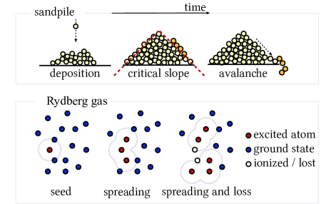
Figure 1: Top: Illustration of the sandpile model. Sand is piling up on a plate via slow deposition ($=$ drive). The sandpile reaches a critical slope at which friction and gravitation balance each other. Further deposition triggers scale invariant avalanches, which deplete at the boundaries ($=$ dissipation). Bottom: Illustration of excitation spreading in a Rydberg gas in the facilitation regime. Excited atoms (red) act as seeds which facilitate the excitation of neighboring atoms that traverse the facilitation shell (gray circles). This leads to spreading of excitations. Ionization or loss of excited atoms yields a depletion of the atom density proportional to the number of excited atoms.

VI.1 Field theory for self-organized criticality

Self-organized criticality is closely linked to absorbing state phase transitions [73, 72, 164, 162, 458, 601, 488, 586, 405]. Both bear the same phenomenology at the critical point: although the stationary density of excitations is zero or infinitesimal, a single, local seed can start an extensive excitation avalanche growing over large parts of the system. Owing to criticality, the size and lifetime of those avalanches follows a scale invariant distribution function [431].

From this viewpoint, SOC can be viewed as a phase transition between an absorbing phase (corresponding to a subcritical slope and a vanishing density of excitations) and an active phase (corresponding to a supercritical slope and a nonzero density of excitations). By the interplay of drive and dissipation, the system is constantly pushed toward the critical point. This can be achieved, for instance, when the drive pushes the system from the absorbing to the active phase, e.g., by depositing sand, and dissipation is conditioned on the active degrees of freedom, e.g., by removing excitation avalanches at the boundary [164]. Thus, self-organized criticality is described by a modified field theory for absorbing state phase transitions such as directed percolation discussed in Sec. V. Here the order parameter $\phi(t,{\bf x})$ again represents the local density of excitations, e.g., forming an avalanche. To the conventional absorbing state field theory, SOC adds the slope field $n(t,{\bf x})$, which acts as a local, dynamical mass $m\to m-n(t,{\bf x})$, i.e., the time-dependent slope around the critical point. An important example is the extension of directed percolation to SOC, for which the order parameter field evolves according to the Langevin equation (cf. Eq. (48)) [73, 72, 164, 162, 96] (we set $\phi\equiv\phi(t,{\bf x}),\eta\equiv\eta(t,{\bf x}),n(t,{\bf x})\equiv n$)

$$\partial_{t}\phi=\left(D\nabla^{2}-m+n\right)\phi-\kappa\phi^{2}+\eta,$$ (50)

with a noise gap $\langle\eta(t,{\bf x})\eta(t^{\prime},{\bf x}^{\prime})\rangle=\delta(t-t^{\prime})\delta({\bf x}-{\bf x}^{\prime})\gamma\phi(t,{\bf x})$. The dynamical mass $n$ obeys the equation of motion

$$\partial_{t}n=\left(D\nabla^{2}-\mu\right)\phi+\delta.$$ (51)

One distinguishes several cases: (i) For $\mu=\delta=0$, the total mass $\int d\mathbf{x}\,n$ is conserved, which corresponds to the Manna model or conserved directed percolation [73, 586]. It describes the dynamics of the Abelian sandpile model if the initial average density is at the critical point. (ii) The case $\mu>0,\delta=0$ corresponds to a model with bulk dissipation, e.g., as in the forest fire model without regrowth [136]. The system may evolve toward a critical point and displays transient critical behavior if $\mu$ is the smallest scale in the theory. Asymptotically, it drops below the critical point and ends up in the absorbing phase [458], featuring a universal dynamics known as dynamical percolation [298]. (iii) For $\mu,\delta>0$ one finds a reloading mechanism, similar to a forest fire model with regrowth. It pushes the system into the active phase, with an average density $\phi=\delta/\mu$, which acts as an effective mass scale. The cases (ii) and (iii) do not display true critical behavior on all length scales due to the remaining scale $\mu$ or $\delta/\mu$. These dynamics may appear self-organized critical on large time and length scales [328] and thus has been termed self-organized quasi-critical [73].

The universal scaling exponents of SOC are related to the size and lifetime of excitation avalanches. Denoting by $s$ the maximum spatial extension of a given avalanche and by $t_{\ell}$ its lifetime, and the respective distribution functions by $P(s)$ and $P(t_{\ell})$, the scaling exponents $\alpha$, $\tau$, and $\gamma$ are defined as follows:

$$P(s)\sim s^{-\tau},\quad P(t_{\ell})\sim t_{\ell}^{-\alpha},\quad\langle s\rangle_{t_{\ell}}\sim t_{\ell}^{\gamma}.$$ (52)

The scaling exponents are unique for a unique absorbing state, e.g., for the sandpile model and for the conserved directed percolation model, but have been shown to vary for models with multiple absorbing states [431, 73]. This indicates that the cases (ii) and (iii) defined above may not display unique scaling exponents, and instead $\alpha$, $\tau$, and $\gamma$ may depend on $\delta,\mu$. However, no such dependence was found in Ref. [328].

VI.2 Self-organized criticality in Rydberg atom ensembles

In experiments with Rydberg gases in the facilitation regime, excitation avalanches have been observed in several different setups [238, 74, 548, 196, 282, 170]. Recently, signatures of self-organized criticality, i.e., the self-organization toward a unique density of atoms and a scale invariant distribution of excitation avalanches, have been reported [282, 170, 331]. At the heart of this connection is a conditioned loss mechanism: excited atoms in the Rydberg state have a small probability to become ionized and to subsequently escape from the trap. The average number of potential facilitation partners thus decays, and the local decay rate is proportional to the number of excited, i.e., active, atoms. The average number of partners, i.e., the local Rydberg atom density $n(t,\mathbf{x})$, is the Rydberg-equivalent of the dynamical mass, and it experiences bulk dissipation as in Eq. (51) through the loss of excited atoms [170, 282, 328, 331]. Thus we have the translation table

order parameter: $$\phi(t,\mathbf{x})=\frac{1}{V_{{\bf x}}}\sum_{l\in V_{\bf x}}\langle\hat{n}_{l}(t)\rangle\text{ [excitation density]},$$

dynamical mass: $$n(t,{\bf x})=\frac{1}{V_{{\bf x}}}\sum_{l\in V_{\bf x}}\langle 1-\hat{n}_{l}(t)\rangle\text{ [atom density]}.$$

In a typical experiment, a gas of Rydberg atoms is cooled down to low temperatures ($\leq 10\,\mu$K) and confined in an optical trap, e.g., an isotropic Gaussian potential $V\sim-\sum_{l}\exp(-\mathbf{x}_{l}^{2}/w^{2})$ with width $w$. The vector $\mathbf{x}_{l}$ is the position of atom $l$ with respect to the origin of the trap. The atoms undergo thermal motion, and after a short equilibration period the average atom density $n(t,{\bf x})$ follows approximately the trapping potential. In this case, the Ising-type Hamiltonian for the driven Rydberg ensemble in Eq. (41) does not depend on discrete lattice positions but on the continuously varying spatial coordinates of each atom $\mathbf{x}_{l}$. Facilitation dynamics are enabled by applying an excitation laser with large detuning ($|\Delta|\gg\Omega$): single-particle processes are strongly suppressed, while resonant excitations take place in the facilitation shell, where the van der Waals interaction $V_{lm}=C_{6}/|\mathbf{x}_{l}-\mathbf{x}_{m}|^{6}$ compensates the detuning $\Delta$, see Fig. 1.

In free space, the number of atoms contributing to facilitation during a time interval $t$ is given by the number of atoms that are traversing the facilitation shell of an excited atom during this interval. It thus increases proportionally to the atom density, which after appropriate coarse graining [328, 331, 282] yields a modification to the Langevin equation Eq. (48) (we set $\phi\equiv\phi(t,\mathbf{x}),n\equiv n(t,\mathbf{x}),\eta\equiv\eta(t,\mathbf{x})$)

$$\partial_{t}\phi=\left(D\nabla^{2}-m+\kappa n/2\right)\phi-\kappa\phi^{2}+\eta.$$ (53)

Instead of a fixed mass $m$, which depends only on the coordination number, the spreading rate depends on the local atom density $n$. This is equivalent to the Langevin equation (50) for SOC with the dynamical mass $n\to\kappa n/2$ rescaled by a constant decay rate.

The evolution of the atom density is determined by two physical processes: (i) the motion of the atoms in the trap, which may be described by a continuity equation [331], and (ii) the total loss of atoms from ionization. The latter is conditioned on the Rydberg state, i.e., it is proportional to the excitation density $\phi$. It yields the evolution

$$\partial_{t}n=\nabla\cdot\left(D\nabla+\mathbf{F}\right)n-\mu\phi.$$ (54)

This differs from Eq. (51) in that $n$ generates its own dynamics, composed of a homogeneous diffusion term $\sim D$ and an effective “force” $\mathbf{F}({\bf x})\sim\nabla V({\mathbf{x}})$, set by the trapping potential.

For a homogeneous gas, $V(\mathbf{x})=0$, Eqs. (50) and (54) yield a behavior similar to the forest fire model without regrowth. The atom density $n$ at large times drops below its critical value, leaving a transient time window at which excitation avalanches can be observed. This sets a natural cutoff scale for the lifetime and the size of avalanches, which depends on the loss rate and the critical density of atoms [328, 331].

In general, however, the trap is not homogeneous $V(\mathbf{x})\neq 0$, and the atoms tend to distribute themselves diffusively according to the trapping profile. This may yield a competition between the atom motion, aiming to pile up atoms in the center of the trap, and the loss from the Rydberg state, removing atoms in the regimes of strong facilitation, i.e., of high density (large dynamical mass) $n$. If the central region of the trapped gas is in the self-organized critical regime, this leads to an observable, flat density profile, with the average density being close to the critical value $\langle n\rangle\approx\gamma/\kappa$, see Fig. 2. Instead of dropping below the critical value eventually, the density is replenished by atoms moving from the flanks of the trapped gas to the center [282, 331]. Over time, this leads to a shrinking, or melting of the cloud, until no further facilitation is possible. Both the formation of a ”flat-top” density distribution and the melting of the cloud have been identified in Rydberg experiments and in theory [331] and, in addition to the observation of avalanches, provide further evidence of self-organized critical behavior in Rydberg ensembles. A similar compensation mechanism has been identified in the atomic vapour experiments [170].

Despite the range of theoretical results and the experimental evidence of a scale invariant avalanche distribution (with measured exponent $\tau=1.37$), the universality class of the Rydberg gas-variant of SOC, described by Eqs. (53), (54), has yet to be determined. Although the order parameter dynamics are equivalent to both the sandpile and the forest fire model, the evolution of the dynamical mass scale differs from any previously proposed theory for SOC. One may see it as a reversed scenario compared to the Abelian sandpile model: In the Rydberg setup, bulk dissipation (the loss of excited atoms) is compensated by a boundary drive (atomic currents from the flanks toward the center), whereas in the Abelian sandpile model boundary dissipation (avalanches lost at the edges) is compensated by bulk driving (the deposition of sand).

One may ask to what extent the dynamical mass can modify the universal behavior, i.e., the critical exponents, of self-organizing systems. Deliberately manipulating the dynamical mass may be a way to realize different classes of self-organizing dynamics in open cold atom systems and to interpolate between, e.g., the paradigmatic sandpile model and more complex scenarios such as the self-organization in neural networks with tissue growth [370, 641].

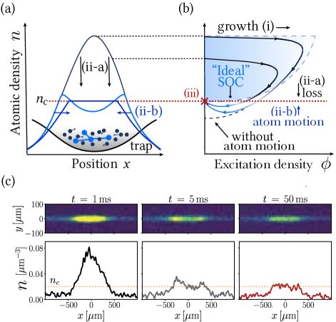
Figure 2: Self-organized criticality in a gas of ultracold Rydberg atoms. (a) Driving an inhomogeneously trapped gas with an off-resonant laser induces the facilitated spreading of excitations (blue dots). (b) Evolution of the density of atoms $n$ ($\equiv n(t,\mathbf{x})$) and the excitation density $\phi$ ($\equiv\phi(t,\mathbf{x})$) from facilitation, loss and atomic motion. The initial supercritical state $n(t=0,\mathbf{x})>n_{c}$ evolves through three stages: (i) fast growth of excitations; (ii-a) self-organization into a critical density due to loss of particles; (ii-b) regrowth of the density in the center due to atomic motion from the flanks toward the center; (iii) the critical point is stabilized on transient time scales. (c) Upper panels: two-dimensional experimental absorption images. Lower panels: reconstructed atom densities along a 1D slice with $y=z=0$. The flat-top coincides with the critical density. Figure adapted from Ref. [331].

VI.3 Alternative sources of scale invariance without fine-tuning in cold atom dynamics

Complex systems host further scenarios, besides SOC, which foster an emergent scale invariant behavior without external fine-tuning. Potential sources are the presence of conservation laws [256, 388], hidden correlations with the environment [524], disorder [254, 432], or dynamical bistabilities [512]. Both disorder and dynamical bistabilities can play a particularly important role for driven-dissipative Rydberg gases. For instance, a dynamical Griffiths phase [432] has been experimentally observed in heterogeneous driven Rydberg gases [615] and theoretical works predict conditions for a self-organized bistable regime [512, 497]. In both cases, scale invariant behavior is enabled by microscopic quantum processes, while at large distances it is governed by semiclassical dynamical equations.

Self-organized bistability (SOB).

SOB refers to a scenario that displays a self-organization mechanism similar to SOC. However, SOB is based on an underlying discontinuous, first order absorbing state phase transition. In this case, the self-organization mechanism does not push the system toward a critical point but rather to a bistability, which separates the absorbing from the active phase [512]. Despite the different nature of the underlying phase transition, both SOC and SOB share similar characteristics, i.e., scale invariant avalanches, differing only in the precise values of the scaling exponents [97].

In Sec. V.2, it was pointed out that the facilitation rate of nearby atoms can be enhanced if multiple excited states are available simultaneously by forming a coherent superposition (cf. the Rydberg superatom [603]). This phenomenon was discussed for Rydberg atoms in a lattice in Eqs. (46), (48). It yields an enhancement of the facilitation rate proportional to the cubic density $\phi^{3}$, cf. the discussion below Eq. (48). In this case, the critical point is replaced by a bistable point, characteristic for a first order phase transition. Although the probability of an atom traversing the facilitation shell of two or more Rydberg atoms simultaneously is strongly suppressed, it may become relevant in dense Rydberg plasmas, such as in Ref. [170]. Tuning the density of Rydberg atoms or their velocity distribution may thus enable to switch between the regimes of SOB and SOC.

Griffiths effects.

Griffiths effects are responsible for the emergence of scale invariant behavior in strongly heterogeneous systems, i.e., systems that are subject to strong spatial fluctuations in their external parameters. Typical examples are quantum and classical magnets [592, 591, 254] or networks with spatially modulated connectivity [432]. Once the scale of the heterogeneity, e.g., the disorder strength, becomes dominant over all other scales, the system breaks up into disconnected or weakly connected clusters. Each cluster has its own time- or energy scale, which largely depends on the (random) size of the cluster. The dynamics of the system as a whole are then determined by the ensemble of approximately independent and equally distributed spatial clusters. In many cases, the ensemble displays scale invariant behavior through the interplay between cluster size distribution and cluster lifetimes (see below) even though each individual cluster is far from any critical point [592, 254]. As a consequence of the latter, the scaling exponents are nonuniversal and vary with the external parameters.

For the dynamics on complex networks, the mechanism leading to Griffiths effects is most transparent: Consider for simplicity a large network of nodes put on a lattice. Any pair of neighboring nodes shall be connected by an edge with probability $p$. When $p=1$, the network is homogeneous and has maximum connectivity. Reducing $p<1$, the network becomes heterogeneous. Imagine a dynamical process, e.g., the contact process in Eq. (46), on this network, such that the dynamics can only pass along connected nodes. Weak heterogeneity then typically yields a perturbative renormalization of the dynamical parameters. Once the heterogeneity of the network, however, becomes significant, the connectivity of the nodes displays strong spatial fluctuations. The dynamics are then governed by the network topology: if the network is percolating, it undergoes a conventional absorbing state phase transition, driven by the competition between spreading and decay of excitations. For strong heterogeneity the network itself undergoes a phase transition: it changes from a percolating network into a nonpercolating one, which hosts only absorbing states.

The nonpercolating network breaks into a set of disconnected clusters without a giant connected component. Each cluster has a finite size $N$ and, as a consequence, can support an active phase only for a finite time scale $\tau_{N}\sim\exp(\alpha N)$ for some $\alpha>0$. Assuming a distribution function $P(N)\sim\exp(-\beta N),\,\beta>0$ of cluster sizes, which decays exponentially for large $N$, the density of excitations on the network is $\phi(t)\sim\int dNP(N)\exp(-t/\tau_{N})\sim t^{-\beta/\alpha}$. It features a scale invariant relaxation with a nonuniversal, continuously varying exponent. Such dynamics are common for complex networks and appears, e.g., in marketing [42], finance [461], informatics [322], and traffic flow [507]. It is a manifestation of a dynamical Griffiths phase [592, 432, 28].

Griffiths phases with a variable decay exponent and signatures of heterogeneity have been observed in gases of Rydberg atoms [615, 75]. In a gas, the atoms move freely and facilitation becomes a dynamical process. It takes place whenever ground state atoms pass the facilitation shell of an excited atom. In order to understand the origin of heterogeneity, consider two atoms with relative velocity $\mathbf{v}$. The relative distance $\mathbf{x}$ between them is $\mathbf{x}=\mathbf{v}t+\mathbf{x}_{0}$. Let $\mathbf{x}_{0}$ be on the facilitation shell, $\Delta=C_{6}/|\mathbf{x}_{0}|^{6}$. Close to $\mathbf{x}=\mathbf{x}_{0}$, this yields the Hamiltonian

$$\hat{H}=\left(\frac{C_{6}}{|\mathbf{x}_{0}+\mathbf{v}t|^{6}}-\Delta\right)\sigma^{z}+\frac{\Omega}{2}\sigma^{x}\approx At\sigma^{z}+\frac{\Omega}{2}\sigma^{x},$$ (55)

with $A=\frac{6\Delta\mathbf{v}\mathbf{x}_{0}}{|\mathbf{x}_{0}|^{2}}$. This is reminiscent of the Landau-Zener problem: the particle undergoes adiabatic passage if it remains in the instantaneous eigenstate. Here, the adiabatic transition corresponds to a ‘spin-flip’, i.e., to a transition from the atomic ground state to the Rydberg state (or vice versa). The adiabatic transition takes place when the relative velocity of the atoms is below a parameter dependent Landau-Zener velocity $v_{\text{LZ}}$. This imposes an additional velocity constraint $|\mathbf{v}|\leq v_{\text{LZ}}$. The likeliness for the constraint to be fulfilled depends on the velocity distribution of the atoms. If the probability $p(|\mathbf{v}|\leq v_{\text{LZ}})$ of finding a particle with velocity $|\mathbf{v}|\leq v_{\text{LZ}}$ is small, a large fraction of atoms is excluded from facilitation, even though they may be spatially close to an excited state. This is equivalent to removing bonds from a facilitation network and to introducing heterogeneity. Depending on the thermal velocity distribution, i.e., the average kinetic energy, the Rydberg atoms form a heterogeneous, effective, facilitation network. The evolution of the Rydberg ensemble can then be described by a heterogeneous rate equation [615] or, on a mean-field level, by a modified Langevin equation [76], which take into account the spatially fluctuating excitation probabilities. The dynamics are then reminiscent of epidemic spreading on complex networks [587, 459, 134, 135, 463, 602, 98].

This discussion shows that the origin of scale invariant behavior on transient and on asymptotic time scales can have various origins in driven quantum systems. What all of the systems share in common is the presence of a fluctuationless dark state. This manifestly modifies the structure of the Keldysh action and results in nonequilibrium scaling behaviors. The construction of scale invariance without fine-tuning, i.e., dynamics featuring a noiseless field configuration and the corresponding vanishing of the action, may be seen as a blueprint for the design of novel types of scale invariant quantum dynamics under drive and dissipation. Conversely, it can be used as a guiding principle to engineer scale invariant dynamics in experiments with driven-dissipative quantum systems, in order to study paradigms of nonequilibrium physics [427].

VII Driven open condensates in low spatial dimensions

The Mermin-Wagner theorem states that two-dimensional (2D) equilibrium systems with short-range interactions and at finite temperature cannot exhibit order that spontaneously breaks a continuous global symmetry [417]. For example, in condensates of interacting bosons in 2D, off-diagonal long-range order is reduced to algebraically decaying correlations due to strong fluctuations of the phase of the condensate. This is a manifestation of the general phenomenon that long-wavelength fluctuations, which lead to the emergence of universal behavior at large scales, are enhanced in low spatial dimensions. A particular aspect of fluctuations of the phase $\theta$ of a condensate lies in its compactness; that is, the property that the phase takes values within a finite interval, $\theta\in[0,2\pi)$, whereby the endpoints of that interval are identified with each other. Compactness implies that the phase field can host topological defects: vortices in 2D and phase slips or space-time vortices in 1D. The proliferation of such topological defects induces the Kosterlitz-Thouless (KT) transition in 2D [337] and the resistive transition in narrow superconducting 1D channels [355, 413]. These results concern systems in thermal equilibrium. Here, we address the question of which novel phase transitions and universal phenomena can be induced out of equilibrium by gapless phase fluctuations and topological defects. This question is of particular relevance for quantum fluids of exciton-polaritons, which have emerged as highly versatile laboratories to study nonequilibrium condensation phenomena in one and two spatial dimensions [160, 120].

VII.1 Long-wavelength theory of driven open condensates

Exciton-polaritons are hybrid quasiparticles that emerge from the strong coupling between light and matter excitations in semiconductor microcavities [120]. Specifically, the direct coherent coupling between cavity photons and excitons or bound electron-hole pairs results in the formation of two bands that are called the upper and lower polaritons, as illustrated in Fig. 3. From their excitonic component, the polaritons inherit screened Coulomb interactions; the leakage of photons through the cavity mirrors leads to a finite lifetime of exciton-polaritons, which necessitates a constant replenishment of their population through a laser drive.

Two possibilities to implement the laser drive are illustrated in Fig. 3: In the incoherent pumping scheme, the laser frequency is chosen to resonantly populate highly excited states. The polaritons generated in this way undergo relaxation through complex scattering processes before they condense in the lower polariton band. Through these scattering processes, all coherence of the exciting laser is lost, and the spontaneous formation of a phase-coherent condensate breaks the $\mathrm{U}_{c}(1)$ symmetry of incoherently pumped systems discussed in Sec. IV.1. In contrast, in the coherent pumping scheme, the coherence of the laser is imprinted on the population of lower polaritons that is excited resonantly by tuning the laser frequency close to the lower polariton dispersion. The coherent laser drive of the lower polariton field explicitly breaks the $\mathrm{U}_{c}(1)$ symmetry, in particular, for the pump mode that is driven resonantly. However, as illustrated in Fig. 3, parametric scattering of polaritons in the pump mode can lead to a high occupation of two additional modes, the signal and idler. While the phase of the pump mode is locked to the laser, these scattering processes are invariant under rotations of the relative phase of the signal and idler modes, and polariton condensation in the signal mode under coherent pumping corresponds to the spontaneous breaking of this $\mathrm{U}(1)$ symmetry. Therefore, in both pumping schemes, the spontaneous breaking of a $\mathrm{U}(1)$ phase rotation symmetry leads to the emergence of a gapless Goldstone mode that is represented by a phase field $\theta$. Below, we review the derivation of the effective long-wavelength description of driven open condensates of exciton-polaritons in terms of this diffusive Goldstone mode. As commonly done in the literature on exciton-polaritons [120], we employ a description of the dynamics of driven open condensates in terms of Langevin equations, which as explained in Sec. IV.3.2 corresponds to the semiclassical limit of Keldysh field theory.

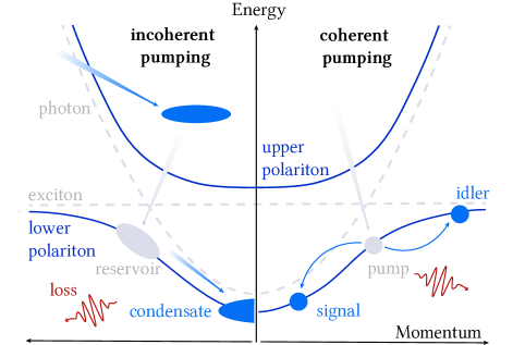
Figure 3: Exciton-polariton dispersion relation and pumping schemes. The coherent coupling of photons and excitons leads to the formation of two bands that are called lower and upper polaritons. Incoherent pumping: Excitations which are injected at high energies undergo relaxation through complex scattering processes and eventually condense at the bottom of the lower polariton branch. Coherent pumping: A laser is tuned close to the inflection point of the lower polariton dispersion relation. Pairs of coherently excited polaritons in the pump mode scatter parametrically into the signal and idler modes. In both pumping schemes, time-continuous pumping is required to compensate losses due to cavity leakage.

VII.1.1 Incoherent pumping scheme and mapping to the compact isotropic KPZ equation

For incoherent pumping, a phenomenological description of the condensate dynamics can be given in terms of two coupled evolution equations for the lower polariton field $\psi(t,\mathbf{x})$ and the excitonic reservoir density $n_{R}(t,\mathbf{x})$. The first equation is a generalized stochastic Gross-Pitaevskii equation that incorporates losses as well as stimulated scattering from the reservoir into the condensate, and the second equation is a rate equation for the reservoir density,

$$\begin{split}i\partial_{t}\psi&=\left(\omega_{\mathrm{LP}}(\hat{\mathbf{q}})-\frac{i}{2}\gamma_{\mathrm{LP}}(\hat{\mathbf{q}})+g_{\mathrm{LP}}\left\lvert\psi\right\rvert^{2}+2g_{R}n_{R}+\frac{i}{2}Rn_{R}\right)\psi+\xi,\\ \partial_{t}n_{R}&=P-\left(\gamma_{R}+R\left\lvert\psi\right\rvert^{2}\right)n_{R}.\end{split}$$ (56)

Here, $\omega_{\mathrm{LP}}(\mathbf{q})$ is the dispersion of lower polaritons illustrated in Fig. 3, and $\hat{\mathbf{q}}=-i\nabla$ is the momentum operator. The dispersion relation can be shaped through band engineering [522]. To obtain a long-wavelength description of the condensate dynamics, an expansion of $\omega_{\mathrm{LP}}(\mathbf{q})$ for small momenta suffices: $\omega_{\mathrm{LP}}(\mathbf{q})=\omega_{0}+q^{2}/(2m_{\mathrm{LP}})$ with $q=\left\lvert\mathbf{q}\right\rvert$. This also applies to the momentum-dependent loss rate, which can be expanded as $\gamma_{\mathrm{LP}}(\mathbf{q})=\gamma_{\mathrm{LP},0}+\gamma_{\mathrm{LP},2}q^{2}$. The momentum dependence of the loss rate is often omitted but can be crucial to ensure the stability of the condensate [36]. Furthermore, $g_{\mathrm{LP}}$ is the polariton-polariton interaction strength, and the term $2g_{R}n_{R}$ describes repulsive interactions between polaritons and reservoir excitons. We assume that the rate of pumping $P$ into the excitonic reservoir is spatially homogeneous on the scales of interest. Reservoir excitons either relax into the polariton condensate by stimulated scattering with rate $R$, or they decay through other channels at the rate $\gamma_{R}$. Finally, as in Eq. (39), $\xi(t,\mathbf{x})$ describes Gaussian noise induced by loss and laser drive. The noise field has a vanishing mean value and its fluctuations are given by $\langle\xi(t,\mathbf{x})\xi^{*}(t^{\prime},\mathbf{x}^{\prime})\rangle=\left(\gamma_{\mathrm{LP},0}+Rn_{R}\right)\delta(t-t^{\prime})\delta(\mathbf{x}-\mathbf{x}^{\prime})$.

Through adiabatic elimination of the excitonic reservoir, which is valid in the absence of dynamical instabilities [71, 68, 69, 36, 70, 584], the generalized Gross-Pitaevskii equation (56) can be reduced to a Langevin equation for the condensate field of the form of Eq. (39). The spatially homogeneous and noiseless mean-field solution of this Langevin equation takes the form $\psi=\sqrt{\rho_{0}}e^{i\theta}$ where $\rho_{0}=-r_{d}/u_{d}=-r_{c}/u_{c}$, with the second equality being satisfied in a suitably chosen rotating frame. Fluctuations of the condensate density are gapped and can be integrated out. Consequently, the dynamics of the condensate phase are described by the compact KPZ (cKPZ) equation [257, 255, 18, 231, 303, 278],

$$\partial_{t}\theta=D\nabla^{2}\theta+\frac{\lambda}{2}\left(\nabla\theta\right)^{2}+\eta,$$ (57)

where

$$\lambda=-2K_{c}\left(1-\frac{K_{d}u_{c}}{K_{c}u_{d}}\right).$$ (58)

Formally, Eq. (57) is equivalent to the noncompact KPZ equation. However, solutions to the cKPZ equation can also contain discontinuous jumps by multiples of $2\pi$ as are encountered, e.g., in 2D upon encircling a vortex.

As explained in Sec. IV.3.2, the Keldysh action that corresponds to the Langevin equation (39) obeys the thermal symmetry introduced in Sec. III.2 only if $K_{c}/K_{d}=u_{c}/u_{d}$, which implies $\lambda=0$. For a pumped nonequilibrium system, these relations correspond to unphysical fine-tuning. Generically, $\lambda\neq 0$, and $\lambda$ serves as a single-parameter measure of the strength of nonequilibrium conditions. The sign of $\lambda$ is irrelevant because it can be absorbed in a redefinition of $\theta$ and the noise field $\eta$. In contrast, the diffusion coefficient $D>0$ has to be positive to ensure dynamical stability. The diffusion coefficient $D$ and the strength $\Delta$ of the noise field $\eta$, which has vanishing mean and fluctuations $\langle\eta(t,\mathbf{x})\eta(t^{\prime},\mathbf{x}^{\prime})\rangle=2\Delta\delta(t-t^{\prime})\delta(\mathbf{x}-\mathbf{x}^{\prime})$, are given by

$$D=K_{c}\left(\frac{K_{d}}{K_{c}}+\frac{u_{c}}{u_{d}}\right),\quad\Delta=\frac{\gamma}{2\rho_{0}}\left(1+\frac{u_{c}^{2}}{u_{d}^{2}}\right).$$ (59)

We have outlined the derivation of the cKPZ equation (57) from the Langevin equation for the condensate, but the cKPZ equation can also be obtained by integrating out density fluctuations within the Keldysh formalism [541]. Further, the coupled equations (56) can be mapped to the cKPZ equation without adiabatic elimination of the excitonic reservoir [204]. This leads to a renormalization of the parameters of the cKPZ equation, which does not affect the long-wavelength behavior but can be significant for quantitative comparisons to numerics and experiments. Conversely, if one is interested only in the correct form of the long-wavelength description and not in quantitative accuracy of the coefficients, it is possible to derive Eq. (57) from only a few fundamental principles: (i) Spontaneous breaking of a $\mathrm{U}(1)$ symmetry leads to the existence of a gapless Goldstone mode, and the evolution equation of a gapless mode may contain only derivative terms. Further, in an expansion in derivatives as appropriate in the long-wavelength and low-frequency limit, we can restrict ourselves to the lowest-order and thus most relevant terms that are allowed by symmetry. (ii) Rotational symmetry implies that there are no terms that contain only a single spatial derivative such as $\mathbf{B}\cdot\nabla\theta$. (iii) In equilibrium, a term such as $\left(\lambda/2\right)\left(\nabla\theta\right)^{2}$, which cannot be written in the form $\delta\mathcal{F}/\delta\theta$, i.e., as the variational derivative of a free energy functional $\mathcal{F}[\theta]$, is forbidden. However, out of equilibrium it is allowed. In particular, this term contains the same number of spatial derivatives as the diffusion term $D\nabla^{2}\theta$ and is, therefore, equally relevant. (iv) In the absence of particle number conservation, the leading temporal derivative is of first order, which leads to diffusive dynamics of the phase when $\lambda=0$. Combining (i)–(iv), we are led to Eq. (57). Instead, if the number of particles is conserved, there is a coherently propagating sound mode, which is correctly described by exchanging the first derivative with respect to time by a second derivative [286].

VII.1.2 Coherent pumping scheme and mapping to the compact anisotropic KPZ equation

In the coherent pumping scheme, lower polaritons are excited directly through a driving field $F(t,\mathbf{x})=F_{0}e^{i\left(\mathbf{q}_{p}\cdot\mathbf{x}-\omega_{p}t\right)}$ with amplitude $F_{0}$ and pump wave vector $\mathbf{q}_{p}$, whereby $q_{p}=\lvert\mathbf{q}_{p}\rvert$ is typically chosen close to the inflection point of the lower polariton dispersion relation shown in Fig. 3, and $\omega_{p}=\omega_{\mathrm{LP}}(\mathbf{q}_{p})$. While the derivation of the cKPZ equation for incoherent pumping presented in the previous section is formally valid in any spatial dimension and relevant for exciton-polaritons in 2D and 1D, for the case of coherent excitation, we focus on 2D systems. Our starting point is again a Langevin equation for the lower polariton field,

$$i\partial_{t}\psi=\left(\omega_{\mathrm{LP}}(\hat{\mathbf{q}})-\frac{i}{2}\gamma_{\mathrm{LP},0}+g_{\mathrm{LP}}\left\lvert\psi\right\rvert^{2}\right)\psi+F+\xi,$$ (60)

where the noise strength is determined by the loss rate, $\langle\xi(t,\mathbf{x})\xi^{*}(t^{\prime},\mathbf{x}^{\prime})\rangle=\gamma_{\mathrm{LP},0}\delta(t-t^{\prime})\delta(\mathbf{x}-\mathbf{x}^{\prime})$. The driving field $F$ explicitly breaks the symmetry of Eq. (60) under phase rotations $\psi\mapsto\psi e^{i\theta}$. However, as we discuss next, there is an emergent $\mathrm{U}(1)$ symmetry in the dynamics of the three dominant field modes, the pump, signal, and idler.

Depending on the strength of the external pump power, there are two different regimes: In the pump-only regime, only a single mode $\psi_{p}$ with wave vector $\mathbf{q}_{p}$ and frequency $\omega_{p}$ set by the external drive is occupied substantially. In contrast, in the optical parametric oscillator (OPO) regime, pairs of polaritons in the pump mode scatter parametrically to other modes, which can thereby also become highly populated. In the simplest case illustrated in Fig. 3, there are two additional highly populated modes, the signal $\psi_{s}$ and the idler $\psi_{i}$. The respective momenta $\mathbf{q}_{s}$ and $\mathbf{q}_{i}$ and frequencies $\omega_{s}$ and $\omega_{i}$ are determined by the conditions $\mathbf{q}_{s}+\mathbf{q}_{i}=2\mathbf{q}_{p}$ and $\omega_{s}+\omega_{i}=2\omega_{p}$. This situation is described by a three-mode ansatz for the lower polariton field $\psi$,

$$\psi(t,\mathbf{x})=\sum_{m=s,p,i}\psi_{m}(t,\mathbf{x})e^{i\left(\mathbf{q}_{m}\cdot\mathbf{x}-\omega_{m}t\right)},$$ (61)

where the amplitudes $\psi_{m}(t,\mathbf{x})$ incorporate long-wavelength, slow fluctuations around the carrier waves $e^{i\left(\mathbf{q}_{m}\cdot\mathbf{x}-\omega_{m}t\right)}$. Therefore, inserting this ansatz in Eq. (60), filtering in momenta and frequencies around the carrier waves, and keeping only parametric scattering processes, yields three coupled equations for the amplitudes $\psi_{m}(t,\mathbf{x})$. A stability analysis shows that the three-mode ansatz is dynamically stable within a restricted range of pump powers [632, 179]. Outside of this range, parametric scattering leads to the population of more than two additional modes. Here, we focus on the regime in which the three-mode ansatz is stable.

Both in the pump-only and the OPO regime, the phase of the pump mode is locked to the phase of the driving laser. Via parametric scattering, the laser drive fixes also the sum of the phases of the signal and idler modes, but not their difference. Consequently, the equations for the amplitudes $\psi_{m}(t,\mathbf{x})$ are invariant under a simultaneous phase rotation of signal and idler modes, $\psi_{s}\mapsto\psi_{s}e^{i\theta}$ and $\psi_{i}\mapsto\psi_{i}e^{-i\theta}$. This U(1) symmetry is broken spontaneously when the pumping strength is varied to cross the threshold to the OPO regime [558, 53, 565, 618], and the associated Goldstone mode governs the long-wavelength dynamics of the OPO condensate. To obtain the corresponding long-wavelength theory, we proceed in two steps: First, we integrate out massive fluctuations, i.e., the density fluctuations of the modes $\psi_{m}$ and the phase fluctuations apart from the relative signal-idler phase $\theta=\theta_{s}-\theta_{i}$ [632]. Second, we expand the lower polariton dispersion $\omega_{\mathrm{LP}}(\mathbf{q})$ around each mode with momentum $\mathbf{q}_{m}$ up to second order in the gradient $\hat{\mathbf{q}}=-i\nabla$,

$$\omega_{\mathrm{LP}}(\mathbf{q}_{m}+\hat{\mathbf{q}})\approx\omega_{\mathrm{LP}}(\mathbf{q}_{m})+\mathbf{B}_{m}\cdot\hat{\mathbf{q}}+\frac{1}{2}\hat{\mathbf{q}}^{{\mathchoice{\raisebox{0.0pt}{$\displaystyle\intercal$}}{\raisebox{0.0pt}{$\textstyle\intercal$}}{\raisebox{0.0pt}{$\scriptstyle\intercal$}}{\raisebox{0.0pt}{$\scriptscriptstyle\intercal$}}}}L_{m}\hat{\mathbf{q}},$$ (62)

where $\mathbf{B}_{m}=\nabla_{\mathbf{q}}\omega_{\mathrm{LP}}(\mathbf{q}_{m})$ and $L_{m}=\nabla_{\mathbf{q}}\nabla_{\mathbf{q}}^{{\mathchoice{\raisebox{0.0pt}{$\displaystyle\intercal$}}{\raisebox{0.0pt}{$\textstyle\intercal$}}{\raisebox{0.0pt}{$\scriptstyle\intercal$}}{\raisebox{0.0pt}{$\scriptscriptstyle\intercal$}}}}\omega_{\mathrm{LP}}(\mathbf{q}_{m})$. The first order contribution $\mathbf{B}_{m}\cdot\hat{\mathbf{q}}$ can be removed by transforming to a frame of reference that moves at a finite velocity $\mathbf{v}$ according to $\theta(t,\mathbf{x})\to\theta(t,\mathbf{x}+\mathbf{v}t)$. At second order, the spatial anisotropy imposed on the system by the pump wave vector $\mathbf{q}_{p}$ manifests in two distinct eigenvalues of the matrix $L_{m}$. Consequently, the long-wavelength description of the Goldstone mode $\theta$ is given by an anisotropic cKPZ equation,

$$\partial_{t}\theta=\sum_{i=x,y}\left[D_{i}\partial_{i}^{2}\theta+\frac{\lambda_{i}}{2}\left(\partial_{i}\theta\right)^{2}\right]+\eta,$$ (63)

where $D_{x}\neq D_{y}$ and $\lambda_{x}\neq\lambda_{y}$. A convenient measure for the degree of spatial anisotropy is provided by the anisotropy parameter $\Gamma$ which is defined as

$$\Gamma=\frac{D_{x}\lambda_{y}}{D_{y}\lambda_{x}}.$$ (64)

In particular, when $\Gamma=1$, the anisotropic cKPZ equation (63) can be reduced to the isotropic KPZ equation (57) through an anisotropic scale transformation. The sign of $\Gamma$ distinguishes between the weakly and strongly anisotropic regimes for $\Gamma>0$ and $\Gamma<0$, respectively. For OPO polaritons, the parameters $D_{x,y}$ and $\lambda_{x,y}$ depend in a nontrivial way on the microscopic system parameters and can be varied substantially by changing the pump strength, the pump momentum $\mathbf{q}_{p}$, and detuning between photons and excitons at zero momentum [632]. In particular, it is possible to reach both the strongly anisotropic regime, and a regime in which the nonequilibrium strengths $\lambda_{x,y}$ become dominant.

VII.2 KPZ universality in the absence of topological defects

The isotropic and anisotropic KPZ equations have originally been introduced to describe the kinetic roughening of growing interfaces [316, 616, 343, 269]. However, physical manifestations of KPZ universality occur in a much wider variety of systems [561] ranging from liquid crystals [563] to burning paper [412], the growth of bacterial colonies [12], and urban skylines [439], but also in the growth of entanglement in random quantum circuits [437] and in spin transport [605, 319]. All of these examples are described by the noncompact KPZ equation. In contrast, the long-wavelength dynamics of driven open condensates and also of a variety of other systems ranging from driven vortex lattices in disordered superconductors [25], to polar active smectics [127], synchronization in oscillator arrays [359, 261], and limit-cycle phases that emerge from a Hopf bifurcation [362, 387, 307, 125, 519], are described by the cKPZ equation. Before we discuss deviations from KPZ universality due to compactness, we review predictions for the expected scaling in the condensate coherence based on an RG analysis of the noncompact KPZ equation [316, 616, 127].

VII.2.1 RG flow of the KPZ equation in 1D, 2D, and 3D

In the absence of topological defects, the compactness of the phase field $\theta$ can be neglected. Then, the KPZ equation (57) can be brought to a dimensionless form through the following rescaling, in $d$ spatial dimensions, where $\Lambda$ is the ultraviolet (UV) momentum cutoff:

$$\mathbf{x} \to\frac{\mathbf{x}}{\Lambda}, t \to\frac{t}{\Lambda^{2}D},$$ (65)

$$\theta \to\theta\sqrt{\frac{\Delta}{\Lambda^{2-d}D}}, \eta \to\eta\sqrt{\Lambda^{2+d}D\Delta}.$$

In the rescaled form of the KPZ equation, the only remaining independent parameter is the dimensionless nonequilibrium strength defined as $g=\Lambda^{d-2}\lambda^{2}\Delta/D^{3}$ [566]. Its canonical scaling dimension $2-d$ determines the large-scale behavior of the theory:

• In 3D, the dimensionless nonequilibrium strength $g$ is irrelevant, and, for sufficiently small microscopic values of $g$, effective equilibrium is emergent at large scales (see the discussion in Sec. III.3).

• In 2D, the canonical scaling dimension of $g$ vanishes, and the loop correction renders the nonequilibrium strength marginally relevant.

• In 1D, $g$ is relevant and grows under renormalization until the canonical flow is balanced by the loop correction at a strong-coupling fixed point.

1D and 2D condensates are thus unstable against small nonequilibrium perturbations that occur on a microscopic scale—these perturbations will grow under coarse graining. Consequently, the long-distance scaling properties of these systems are strongly modified under nonequilibrium conditions. In particular, KPZ scaling becomes manifest in the spatial coherence as measured through the correlation function or Keldysh Green’s function $C(t-t^{\prime},\mathbf{x}-\mathbf{x}^{\prime})=\langle\psi(t,\mathbf{x})\psi^{*}(t^{\prime},\mathbf{x})\rangle\approx\rho_{0}e^{-\langle\left(\theta(t,\mathbf{x})-\theta(0,0)\right)^{2}\rangle/2}$, where in the approximation we have neglected fluctuations of the density and treated fluctuations of the phase to leading order in a cumulant expansion. The RG analysis of the KPZ equation leads to [566]

$$\langle\left(\theta(t,\mathbf{x})-\theta(0,0)\right)^{2}\rangle\sim\begin{cases}r^{2\chi}&\text{for }r\to\infty,\\ t^{2\beta}&\text{for }t\to\infty,\end{cases}$$ (66)

where $r=\left\lvert\mathbf{x}\right\rvert$. That is, spatial and temporal fluctuations of the condensate phase $\theta$ are determined by the roughness exponent $\chi$ and the growth exponent $\beta$, respectively. In 2D, numerical studies indicate that $\chi\approx 0.39$ and $\beta\approx 0.24$ (see, e.g., Ref. [243] and references therein); in 1D, the exponents take the exact values $\chi=1/2$ and $\beta=1/3$. The roughness and growth exponents are interdependent through the scaling relation $\chi+z=2$ which holds at any nontrivial and finite fixed point of $g$, and where $z=\chi/\beta$ is the dynamical exponent [566]. For the condensate correlation function, Eq. (66) implies stretched-exponential decay both with spatial and temporal distances. This behavior is in stark contrast to the algebraic decay of correlations in 2D condensates in thermal equilibrium.

The RG analysis provides predictions not only for the universal scaling behavior of the correlation function but also for the length and time scales beyond which KPZ scaling is established. In 2D, the marginality of the dimensionless nonequilibrium strength $g$ implies that the RG flow starting from a small microscopic value $g_{0}\ll 1$ reaches the strong-coupling regime in which KPZ scaling emerges only on exponentially large scales that are greater than

$$L_{\mathrm{KPZ}}=a\,e^{8\pi/g_{0}},$$ (67)

where $a=1/\Lambda$ is the microscopic length scale on which the RG flow is initialized. In contrast, in 1D, the nonequilibrium strength is relevant, and, therefore, the KPZ scaling regime is reached at a scale $L_{\mathrm{KPZ}}\sim 2\pi a/g_{0}$ that is only algebraically large in $g_{0}\ll 1$ [441].

Recently, some aspects of KPZ physics have been observed in synthetic magnetic systems [605]. Importantly, these systems are operated in one dimension and in thermodynamic equilibrium; in 1D, the KPZ nonlinear term, driving the characteristic universality, is accidentally compatible with equilibrium conditions [311, 55, 346], but this is not the case in higher spatial dimensions. Therefore, 2D KPZ universality is a unique promise of nonequilibrium platforms such as those discussed above. We return to this point in Sec. VII.3.4.

VII.2.2 RG flow of the anisotropic KPZ equation in 2D

A new feature of the anisotropic KPZ equation (63) in 2D is that the nonequilibrium strength $g$ becomes irrelevant for sufficiently strong anisotropy. That is, by making the system strongly anisotropic, effective thermal equilibrium and algebraic quasi-long-range order can be restored on large scales. This behavior is encoded in the RG flow of the nonequilibrium strength $g=\lambda_{x}^{2}\Delta/(D_{x}^{2}\sqrt{D_{x}D_{y}})$ and the anisotropy parameter $\Gamma$ defined in Eq. (64) [616, 127],

$$\begin{split}\frac{dg}{d\ell}&=-\frac{g^{2}}{32\pi}\left(\Gamma^{2}+4\Gamma-1\right),\\ \frac{d\Gamma}{d\ell}&=-\frac{\Gamma g}{32\pi}\left(1-\Gamma^{2}\right),\end{split}$$ (68)

where $\ell$ is the logarithm of the running momentum cutoff. The RG flow is markedly different in the regimes of weak and strong anisotropy which correspond to $\Gamma>0$ and $\Gamma<0$, respectively: For weakly anisotropic systems, spatial isotropy and KPZ scaling as described by Eq. (66) are restored on large scales; in contrast, for strong anisotropy, the RG flow is attracted to a fixed point at $g=0$ and $\Gamma=-1$. Since the nonequilibrium strength vanishes at this fixed point, effective thermal equilibrium is established. This leads to logarithmic spatial growth of phase fluctuations [127],

$$\langle\left(\theta(0,\mathbf{x})-\theta(0,0)\right)^{2}\rangle\sim\ln\!\left(\lambda_{y}x^{2}+\lambda_{x}y^{2}\right),$$ (69)

resulting in algebraic quasi-long-range order. As noted below Eq. (62), for coherently driven exciton-polaritons, these results apply in a moving frame of reference. Spatial correlations are not affected by the transformation back to the original frame. However, for temporal correlations this transformation leads to a crossover between different stretched exponential and algebraic scaling regimes for weak and strong anisotropy, respectively [632].

We emphasize that the mechanism of asymptotic thermalization described above hinges on strong spatial anisotropy and is, therefore, profoundly different from asymptotic thermalization in the isotropic KPZ equation in 3D, which results from the irrelevance of $g$ as discussed in Sec. VII.2.1, and also from the other examples for the emergence of equilibrium at large scales mentioned in Sec. VIII.1.

VII.3 Vortex unbinding in two-dimensional driven open condensates

The RG analysis that leads to the predictions for the spatiotemporal coherence of driven open condensates given in Eqs. (66) and (69) ignores the possible occurrence of topological defects. In the theoretical description of 2D condensates in equilibrium, topological defects can be incorporated by employing an electrodynamic duality which maps vortices to electric charges that form a 2D Coulomb gas and rephrases the KT transition as a screening transition [20, 21, 142, 418]: At low temperatures, pairs of vortices and antivortices remain tightly bound due to their attractive interaction; but above the KT critical temperature, strong fluctuations screen the vortex-antivortex interaction at large distances. Then, unbound vortices can move freely through the system and destroy quasi-long-range order. This electrodynamic duality has been extended to isotropic and anisotropic driven open condensates in Refs. [595, 545] and Ref. [540], respectively.

In the absence of vortices, universal KPZ scaling is established beyond the exponentially large scale $L_{\mathrm{KPZ}}$ Eq. (67). A key prediction of the electrodynamic duality is the existence of another exponentially large scale $L_{v}$ associated with the proliferation of vortices in isotropic systems. Therefore, the relative size of $L_{\mathrm{KPZ}}$ and $L_{v}$ determines the observability of KPZ universality in isotropic driven open condensates. We will return to this point in Sec. VII.3.4 below.

VII.3.1 Electrodynamic duality

In the dual description, topological defects and smooth fluctuations of the condensate phase $\theta$ are represented through the coupled dynamics of a gas of point charges and electromagnetic fields. The electric field $\mathbf{E}$ is defined as

$$\mathbf{E}=-\hat{\mathbf{z}}\times\nabla\theta,$$ (70)

where $\hat{\mathbf{z}}$ is a unit vector normal to the 2D plane that supports the condensate. An overdamped version of Farady’s law relates the electric field to the magnetic field $\mathbf{B}$,

$$\nabla\times\mathbf{E}+\frac{1}{D}\mathbf{B}=0.$$ (71)

Here, we set $D=D_{x}=D_{y}$, which can be achieved through an anisotropic rescaling of the units of length in Eq. (63). From the definition of the electric field in terms of the condensate phase and Faraday’s law it follows that $\mathbf{B}=B\hat{\mathbf{z}}$, which in turn implies $\nabla\cdot\mathbf{B}=0$. Vortices act as sources of the electric field according to Gauss’ law,

$$\nabla\cdot\mathbf{E}=\frac{2\pi}{\varepsilon}n,$$ (72)

where $n(t,\mathbf{x})=\sum_{\alpha}n_{\alpha}\delta(\mathbf{x}-\mathbf{x}_{\alpha}(t))$ is the density of vortices with charges $n_{\alpha}$ at positions $\mathbf{x}_{\alpha}(t)$, and $\varepsilon$ is the dielectric constant that describes screening of the electromagnetic fields due to bound vortex-antivortex pairs. Further, Ampère’s law incorporates the KPZ nonlinearities $\lambda_{x,y}$, the noise $\eta$, and the vortex current $\mathbf{j}(t,\mathbf{x})=\sum_{\alpha}n_{\alpha}\frac{d\mathbf{x}_{\alpha}(t)}{dt}\delta(\mathbf{x}-\mathbf{x}_{\alpha}(t))$,

$$\nabla\times\mathbf{B}-\varepsilon\partial_{t}\mathbf{E}=2\pi\mathbf{j}+\hat{\mathbf{z}}\times\nabla\left(\sum_{i=x,y}\frac{\lambda_{i}}{2}E_{i}^{2}+\eta\right).$$ (73)

For $\mathbf{j}=0$, Ampère’s law reduces to the anisotropic cKPZ equation (63). The above nonlinear and overdamped Maxwell equations can also be derived systematically by discretizing the cKPZ equation on a lattice and performing a modified Villain transformation [545].

To obtain a complete long-wavelength description of the condensate dynamics, the Maxwell equations have to be complemented by an equation of motion for the vortices. Under the assumption of overdamped dynamics, this equation is

$$\frac{d\mathbf{x}_{\alpha}}{dt}=\mu n_{\alpha}\mathbf{E}(\mathbf{x}_{\alpha})+\boldsymbol{\xi}_{\alpha},$$ (74)

where $\mu$ is the phenomenologically introduced vortex mobility. The stochastic force $\boldsymbol{\xi}_{\alpha}$ has vanishing mean, and its correlations are given by $\langle\xi_{\alpha,i}(t)\xi_{\alpha^{\prime},j}(t^{\prime})\rangle=2\mu T\delta_{\alpha,\alpha^{\prime}}\delta_{i,j}\delta(t-t^{\prime})$, where $T$ can be interpreted as an effective vortex temperature which, for systems in thermal equilibrium, is identical to the strength of the noise $\eta$ that enters Ampère’s law.

VII.3.2 Noise-activated vortex unbinding in isotropic systems

To determine the stability of the bound state of a vortex-antivortex pair at distance $\mathbf{x}$, we have to study the screening of the vortex-antivortex interaction due to the polarization of bound pairs of smaller size. Under the assumption that the vortices have low mobility $\mu/D\ll 1$, which should not affect our results qualitatively, the vortex-antivortex interaction can be found in the dual description by solving an electrostatic problem with fixed vortex positions. In doing so, we treat the KPZ nonlinearity perturbatively.

We first consider isotropic systems with $\lambda_{x}=\lambda_{y}$ in Eq. (73). Then, the vortex-antivortex interaction is a conservative force that can be derived from the potential [595]

$$V(\mathbf{x})=\frac{1}{\varepsilon}\ln(r/a)-\frac{\lambda^{2}}{6\varepsilon^{3}D^{2}}\left(\ln(r/a)^{3}+\frac{3}{4}\ln(r/a)^{2}\right),$$ (75)

where $a$ is a microscopic cutoff. That is, at second order in $\lambda$, the logarithmic 2D Coloumb potential acquires a repulsive correction that becomes dominant on distances greater than

$$L_{v}=a\,e^{2D/\lvert\lambda\rvert},$$ (76)

where we have set the dielectric constant to its microscopic value $\varepsilon=1$. The perturbative expansion Eq. (75) in powers of $\lambda\ln(r/a)$ breaks down at distances $r\gg L_{v}$. However, studies of the complex Ginzburg-Landau equation, corresponding to Eq. (39) without noise, indicate that the repulsive vortex-antivortex interaction on distances $r\gtrsim L_{v}$ is exponentially suppressed for $r\gg L_{v}$ [25]. Consequently, even without taking the screening of the vortex-antivortex interaction due to bound pairs into account, we are led to conclude that the bound state of a vortex-antivortex pair is only metastable, and any finite vortex temperature leads to vortex unbinding. In experiments, the vortex temperature, which we have introduced phenomenologically, is determined by the intrinsic parameters of the system and the external drive and is generically nonzero. Based on the present analysis we should then expect a finite density $\sim 1/L_{v}^{2}$ of unbound vortices. This expectation is corroborated by an RG approach that accounts for the renormalization of the dielectric constant $\varepsilon$ due to the polarization of bound vortex-antivortex pairs [595]. Upon integrating out bound pairs on gradually increasing length scales, the dielectric constant is found to flow to ever larger values, signaling the screening of the vortex-antivortex interaction and the presence of unbound vortices.

VII.3.3 Stabilization of the ordered phase through strong spatial anisotropy

The interplay between nonequilibrium conditions and strong spatial anisotropy leads to a stark modification of the vortex-antivortex interaction [540]. This can be understood already by examining the structure of a single vortex shown in Fig. 4: In the weakly anisotropic regime characterized by $\Gamma=\lambda_{y}/\lambda_{x}>0$, vortices emit waves in the radial direction away from the vortex core, leading to a spiral structure [24]; the radial wave vector vanishes in the strongly anisotropic regime with $\Gamma<0$, which results in a much less pronounced spiral structure with a logarithmic instead of linear dependence of the vortex field on the distance from the vortex core; and in the fully anisotropic case corresponding to $\Gamma=-1$, the radial component of the vortex field vanishes altogether. The exponential screening of the vortex-antivortex interaction on distances $r\gg L_{v}$ in the isotropic case can be understood as a consequence of the radially emitted wave [25]. Therefore, the absence of a radially emitted wave for fully anisotropic vortices implies that the interaction is not screened in this case, and that a phase with bound vortex-antivortex pairs can be stable. Further evidence in support of this expectation is provided by a perturbative calculation of the vortex-antivortex interaction, which is valid on scales $r\lesssim L_{v}$, and shows that strong spatial anisotropy can render the correction to the Coulomb potential in Eq. (75) attractive [540].

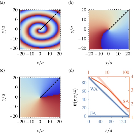
Figure 4: A single vortex in the anisotropic cKPZ equation. Colors from blue to red encode $\theta\in[0,2\pi)$. (a) Weakly anisotropic (WA) regime with $\lambda_{x}/(2D)\approx 0.9$ and $\lambda_{y}/(2D)\approx 0.4$, leading to a pronounced spiral structure. (b) Strongly anisotropic (SA) regime with $\lambda_{x}/(2D)\approx 0.9$ and $\lambda_{y}/(2D)\approx-0.4$, where the radial dependence of the vortex far field is much weaker. (c) Fully anisotropic (FA) configuration with $\lambda_{x}/(2D)=-\lambda_{y}/(2D)\approx 0.7$. The vortex field does not depend on the radial coordinate. (d) The radial dependence of the vortex field along the dashed black lines in (a–c) is $\sim r$ for WA, $\sim\ln(r)$ for SA, and $\sim\mathrm{const.}$ for FA. Straight lines are fits to the numerical data. Figure adapted from Ref. [540].

VII.3.4 Observability of KPZ universality in two-dimensional driven open condensates

Experimentally observing KPZ universality in 2D represents a major challenge due to the scarcity of experimentally accessible 2D interfaces [561]. The finding that driven open condensates belong to the KPZ universality class opens up the intriguing perspective of viewing the condensate phase as such an interface. However, the observability of KPZ universality in driven open condensates critically depends on the absence of unbound vortices. Therefore, we have to compare the characteristic length scales $L_{\mathrm{KPZ}}$ and $L_{v}$ given in Eqs. (67) and (76), which determine the onset of KPZ scaling and the mean separation between unbound vortices, respectively. Both are exponentially large in systems that are driven only weakly out of equilibrium with $\left\lvert\lambda\right\rvert\ll D$; but crucially, $L_{\mathrm{KPZ}}$ and $L_{v}$ are exponentially large in $D^{2}/\lvert\lambda\rvert^{2}$ and $D/\lvert\lambda\rvert$, respectively, such that generically $L_{v}\ll L_{\mathrm{KPZ}}$, indicating that the proliferation of free vortices always preempts the emergence of KPZ scaling. Surprisingly, recent numerical studies show that this does not have to be the case, making the observation of 2D KPZ universality with driven open condensates a tantalizing possibility [415, 158, 195].

Early experimental and numerical studies of the coherence properties of 2D driven open condensates have focused on parameter regimes for which the scales $L_{\mathrm{KPZ}}$ and $L_{v}$ are much larger than the considered system sizes, and, therefore, have observed equilibrium-like behavior characterized by algebraic quasi-long-range order and a vortex-unbinding transition to a disordered phase [502, 445, 148, 345, 111, 140, 234, 630, 139, 149, 147]. More recently, numerical studies have started exploring the far-from-equilibrium regime in which KPZ universality is expected to emerge. Indeed, in Ref. [415], spatial and temporal correlations have been found to be governed on large scales by KPZ scaling exponents in incoherently pumped exciton-polaritons in a regime of weak interactions and weak noise. On short scales, algebraic order is observable even in the absence of interactions—in stark contrast to Bose gases in thermal equilibrium. These coherence properties have been observed in simulations without vortices, while the presence of vortices in the initial state has been found to lead to the proliferation of vortices in the steady state. In Ref. [158], the formation of free vortices has been shown to be strongly suppressed in spatially discrete condensates in a lattice of micro-pillars. This setup has also enabled the experimental observation of KPZ universality in 1D as detailed below [204]. In 2D, vortex creation is suppressed for incoherent pump strengths far above the condensation threshold, and even for experimentally realistic noise strengths. Under these conditions, KPZ universality has been observed both in spatial and temporal correlations and in the distribution of phase fluctuations. Furthermore, KPZ universality of correlations and phase fluctuations has also been demonstrated numerically in coherently pumped exciton-polaritons in an experimentally realistic parameter regime identified in Ref. [632], where $g=\lambda^{2}\Delta/D^{3}\gtrsim 1$ such that $L_{\mathrm{KPZ}}\approx a$, and with weak spatial anisotropy [195]. Remarkably, the strongly nonequilibrium regime considered in these simulations has been found to be stable against the proliferation of vortices, even though Eq. (76) suggests that $L_{v}\approx a$ for the chosen parameters. The mechanism that underlies this increased stability against vortex proliferation is not fully understood but appears to be rooted in the interplay between fluctuations of the amplitude and the phase of the condensate that is not captured by the adiabatic elimination of density fluctuations leading to the cKPZ equation. This assumption is supported by a numerical study of the cKPZ equation on a lattice, which has confirmed key predictions of the electrodynamic duality, including the proliferation of vortices in the steady state in weakly anisotropic systems beyond a length scale that depends exponentially on the inverse of $\left\lvert\lambda\right\rvert$, and the stability of the ordered phase in strongly anisotropic systems [631]. Repulsive vortex-antivortex interactions in isotropic systems have also been observed in simulations of the full complex condensate field [232], and have been found to strongly decrease the rate of vortex-antivortex annihilation [204, 233].

The numerical studies summarized above show that using the condensate phase as an interface which grows according to the KPZ equation is a promising route toward the experimental observation of KPZ universality in 2D, and provide clear guidance concerning the optimal choice of parameters. Another intriguing aspect of driven open condensates, which deserves further numerical and experimental investigations, is the stabilization of algebraic quasi-long-range order through strong spatial anisotropy.

VII.4 One-dimensional driven open condensates

A crucial difference between the noncompact and the compact KPZ equations lies in the fact that the former depends on a single tuning parameter, which is given by the dimensionless nonequilibrium strength $g$, while the latter is determined by two independent parameters. Indeed, the compactness of $\theta$ renders its rescaling in Eq. (65) meaningless. Accordingly, after rescaling $\mathbf{x}$ and $t$ as in Eq. (65), and the noise field as $\eta\to\eta\Lambda^{2}D$, we are left with two independent parameters, which can be chosen as the dimensionless nonequilibrium strength and the dimensionless noise strength defined as $\tilde{\lambda}=\lambda/D$ and $\tilde{\sigma}=\Lambda^{d-2}\Delta/D$, respectively. As shown in Ref. [279] for a 1D driven open condensate, both parameters are associated with new phenomena beyond the physics of the noncompact KPZ equation: The noise strength gives rise to a time scale that terminates the time window during which KPZ scaling can be observed in autocorrelation functions; and increasing the nonequilibrium strength $\tilde{\lambda}$ induces a first order transition to a new phase of space-time vortex turbulence. The phase diagram of 1D driven open condensates, obtained from numerical simulations of the Langevin equation (39) for the condensate field, is illustrated schematically in Fig. 5(a). Another mechanism by which KPZ scaling can disappear is revealed through simulations of the coupled dynamics of a condensate of lower polaritons and an excitonic reservoir as described by Eq. (56) [584]: At high pump powers, the adiabatic elimination of the reservoir, which underlies the description of the dynamics in terms of a single evolution equation for the condensate field, breaks down. Then, strong fluctuations of the condensate and reservoir densities go along with the gradual closing of the temporal window of KPZ scaling.

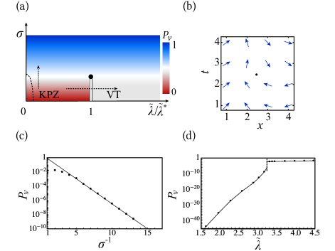
Figure 5: (a) Schematic phase diagram of a 1D driven open condensate in terms of the rescaled nonequilibrium strength $\tilde{\lambda}/\tilde{\lambda}^{*}$ and the noise strength $\sigma$ (denoted by $\gamma$ in Eq. (39)). The color scale encodes the density of vortices in space-time, $P_{v}$. At low nonequilibrium and noise strengths, condensate autocorrelations exhibit KPZ universality. As $\tilde{\lambda}$ is increased beyond the critical value $\tilde{\lambda}^{*}$, a first order transition to a vortex turbulent phase (VT) is crossed. The first order transition line terminates in a second order critical point. (b) Phase configuration for a phase slip at $t\approx 2.5$. The equivalent interpretation as a space-time vortex is apparent. (c) Noise-activated behavior $P_{v}\sim e^{-E_{v}/\sigma}$ along the vertical dashed line in (a). $E_{v}$ is the effective energy of a space-time vortex. (d) The space-time vortex density exhibits a discontinuous jump when $\tilde{\lambda}$ crosses $\tilde{\lambda}^{*}$ along the horizontal dashed line in (a). Figure adapted from Ref. [279].

VII.4.1 KPZ universality in one-dimensional driven open condensates

At weak noise and nonequilibrium strength, the fluctuations of the phase field $\theta$ in the vicinity of any given space-time point are small, and, therefore, the compactness of $\theta$ can be ignored. Then, the correlation function or Keldysh Green’s function $C(t-t^{\prime},x-x^{\prime})=\langle\psi(t,x)\psi^{*}(t^{\prime},x^{\prime})\rangle$ is expected to exhibit KPZ scaling as described by Eq. (66). In 1D, the roughness exponent takes the value $\chi=1/2$ for any value of the KPZ nonlinearity $\lambda$ in Eq. (57), including, in particular, the case $\lambda=0$. However, an unambiguous signature of a significant KPZ nonlinearity, which in turn roots in the breaking of the thermal symmetry in a driven open condensate as discussed in Sec. VII.1.1, is provided by the stretched-exponential decay of the autocorrelation function $C(0,t)\sim\exp(-ct^{2\beta})$ with $\beta=1/3$ for the KPZ universality class. In contrast, $\beta=1/4$ for the Edwards-Wilkinson universality class corresponding to diffusion described by Eq. (57) with $\lambda=0$. KPZ scaling has been observed in numerical studies of the Langevin equation (39) for incoherently pumped driven open condensates in the regime of weak noise, defined by the absence of space-time vortices on the spatiotemporal extent of the simulation [231, 303, 278]. Further evidence comes from simulations of the coupled dynamics of the condensate and reservoir as described by Eq. (56) [204, 584], and from numerics for 1D photonic cavity arrays [22].

The spatiotemporal coherence of exciton-polariton condensates is determined by the second moment of the distribution of phase fluctuations, which exhibit universal KPZ scaling as described by Eq. (66). Signatures of KPZ dynamics beyond scaling are contained in the full distribution of the phase, which follows the Tracy-Widom form during the growth regime of KPZ dynamics [204, 554, 159] before it crosses over to Baik-Rains statistics in the stationary KPZ regime [554]. Moreover, subclasses of KPZ universality, which share the same scaling exponents but are characterized by different variants of the phase distribution and the spatial correlations of phase fluctuations, are accessible in systems with external confinement [159].

Recently, KPZ universality has been demonstrated in an experimental study of a 1D condensate of exciton-polaritons [204]. Observing KPZ universality requires sufficiently spatially extended condensates to avoid finite-size effects, and this requirement poses a challenge to experiments since large condensates are unstable toward fragmentation [551, 71, 378, 155, 69, 188]. A way to overcome this challenge is provided by band engineering in a lattice system to endow the polaritons with a negative effective mass [36]. In particular, performing experiments with exciton-polaritons in a Lieb lattice of coupled micropillars [522] allowed Ref. [204] to reach larger scales than earlier measurements of coherence [502, 199, 445].

Interferometrically probing the light field that leaks out of the cavity gives direct experimental access to the condensate coherence as measured by the absolute value of the first order correlation function,

$$g^{(1)}(\Delta t,\Delta x)=\frac{\langle\psi^{*}(t+\Delta t,x+\Delta x)\psi(t,x)\rangle}{\sqrt{\langle\left\lvert\psi(t+\Delta t,x+\Delta x)\right\rvert^{2}\rangle\langle\left\lvert\psi(t,x)\right\rvert^{2}\rangle}}.$$ (77)

According to Eq. (66), $\lvert g^{(1)}(\Delta x,\Delta t)\rvert$ is expected to exhibit stretched-exponential decay with $\chi=1/2$ and $\beta=1/3$. These values are well reproduced by fits to the experimental data, leading to $\chi_{\mathrm{exp}}=0.51\pm 0.08$ and $\beta_{\mathrm{exp}}=0.36\pm 0.11$. In particular, only the KPZ value $\beta=1/3$ and not the Edwards-Wilkinson value $\beta=1/4$ lies within the $95\%$ confidence interval around $\beta_{\mathrm{exp}}$. Further experimental evidence for KPZ universality is provided by a collapse of the data for $-2\ln\!\left(\kappa|g^{(1)}(\Delta t,\Delta x)|\right)/\Delta t^{2/3}$, plotted against the rescaled coordinate $y=\Delta x/\Delta t^{2/3}$, onto the KPZ scaling function $F=C_{0}F_{\mathrm{KPZ}}(y/y_{0})$. The values of $F_{\mathrm{KPZ}}$ are tabulated [480], and $C_{0}$ and $y_{0}$ are nonuniversal constants. These results demonstrate that 1D condensates of exciton-polaritons indeed belong to the KPZ universality class, and provide motivation for pursuing experiments to demonstrate KPZ universality in 2D. Recall, however, that observing KPZ universality in 2D requires exponentially large scales and is thus far more challenging than in 1D, where only algebraically large length and time scales are required.

VII.4.2 Destruction of KPZ scaling through noise activated space-time vortices

When local fluctuations of the phase become large due to either strong noise or, as detailed below, strong nonequilibrium conditions, compactness of the phase becomes important also in 1D. In particular, large phase fluctuations can induce phase slips. As illustrated in Fig. 5(b), phase slips are best visualized in analogy to topological defects in 2D as space-time vortices.

Experimental and numerical observations of KPZ scaling of phase fluctuations indicate that phase slips are rare at sufficiently weak noise. The space-time density $P_{v}$ of phase slips can be computed by formalizing the equivalence between phase slips and space-time vortices through the mapping of the $1+1\mathrm{D}$ KPZ equation to the static equilibrium description of a smectic $A$ liquid crystal [240, 242, *Golubovic1994]. This calculation shows that for weak noise, space-time vortices exhibit activated behavior with $P_{v}\sim e^{-E_{v}/T}$, where $E_{v}$ and $\sigma$ are the effective energy and temperature of a space-time vortex [279]. The associated mean temporal separation of space-time vortices gives rise to an exponentially large crossover time scale $t_{c}$: KPZ universality with stretched exponential decay of condensate autocorrelations prevails below $t_{c}$, and is superseded by simple exponential decay beyond $t_{c}$. This crossover has been observed in simulations of the Langevin equation (39), and the activated behavior of $P_{v}$ is illustrated in Fig. 5(c).

VII.4.3 Transition to space-time vortex turbulence

Increasing the nonequilibrium strength $\tilde{\lambda}$ beyond a critical value $\tilde{\lambda}^{*}$ triggers a dynamical instability and induces a first order transition to a phase of vortex turbulence, at any finite noise level [279]. A related dynamical instability has also been observed in simulations of both 1D and 2D arrays of coupled phase oscillators [359], and in the coupled dynamics of the condensate and excitonic reservoir as described by Eq. (56) [584]. The phase transition is signaled by a discontinuous jump of the vortex density $P_{v}$ as shown in Fig. 5(d). Note that $P_{v}$ is finite on both sides of the transition. Therefore, the long-time decay of the autocorrelation function is always exponential. The two phases are distinguished by the density of vortices, in analogy to the liquid-gas transition in thermal equilibrium. As illustrated schematically in Fig. 5(a), for increasing noise strength, the first order line terminates in a second order critical point, where the height $\Delta P_{v}$ of the jump in the vortex density goes to zero, and the derivative of $\Delta P_{v}$ with respect to the noise strength $\sigma$ diverges as $\sim\left\lvert\sigma-\sigma^{*}\right\rvert^{-\kappa}$ with $\kappa\approx 0.63$.

An experimentally accessible signature of the transition is provided by the momentum distribution function $n(q)=\int dx\,e^{-iqx}C(0,x)$ [120]. For large momenta $q$, the momentum distribution function behaves generically as $n(q)\sim q^{-\gamma}$. However, crossing the transition, the value of the exponent $\gamma$ jumps from $\gamma\approx 2$, which is characteristic for noise activated vortices [521], to $\gamma\approx 5$, reminiscent of turbulence.

VIII Driven open criticality

In the previous section, we have discussed how strong gapless fluctuations can prohibit spontaneous symmetry breaking in low spatial dimensions. However, in higher dimensions, stable ordered phases with broken symmetries are possible. As anticipated in the Introduction, the strongest form of universality will then manifest in the critical behavior at the symmetry-breaking phase transition. Here, and in Secs. IX and X, we focus on novel critical behavior that results from the breaking of thermodynamic equilibrium conditions on microscopic scales (cf. Tab. 1).

As a first example, in Sec. VIII.1, we will discuss dynamical criticality at the driven open condensation transition in 3D [543, 544, 567, 541]. The starting point of our analysis is the Keldysh action in the semiclassical limit (38) or the equivalent Langevin equation (39). As explained in Sec. VII.1.1, on large length and time scales the Langevin equation (39) can be mapped to the isotropic compact KPZ equation (57). The canonical scaling analysis of Sec. VII.2.1 has shown that the KPZ nonlinearity Eq. (58), which serves as a measure for the breaking of equilibrium conditions as explained in Sec. IV.3.2, is irrelevant in 3D, indicating that in 3D driven open condensates, thermal equilibrium emerges at large scales. Yet, the breaking of equilibrium conditions on microscopic scales becomes manifest in a new critical exponent that describes the approach to equilibrium. Such a modification of critical behavior is possible for a complex order parameter field, but cannot occur for a real order parameter field that describes Ising order [423, 391]. However, as we discuss in Sec. VIII.2, novel forms of nonequilibrium criticality can occur in the coupled dynamics of two competing Ising order parameters [623].

VIII.1 Bosonic driven open criticality

Dynamical critical behavior at the driven open condensation transition in 3D has been studied using the functional RG [59] and a field-theoretical RG approach [566] in Refs. [543, 544] and Ref. [567], respectively. A review of these works is presented in Ref. [541]. Here, we will content ourselves with a short summary.

The RG analysis of the driven open condensation transition yields the following results:

(i) Asymptotic thermalization: Even though thermal equilibrium conditions as expressed through the relation $K_{c}/K_{d}=u_{c}/u_{d}$ for the coefficients in Eq. (38) are violated explicitly at the microscopic level of the theory, symmetry of the Keldysh action under $\mathcal{T}_{\beta}$ Eq. (14) with an effective inverse temperature $\beta$ emerges at the RG fixed point that describes the condensation transition. Consequently, the static and dynamical critical exponents that govern the asymptotic decay of spatial and temporal correlation functions at large spatial and temporal distances take the same values as in the corresponding equilibrium problem. The emergence of thermal equilibrium at large spatial and temporal scales is a rather general phenomenon [423, 166, 168, 152, 575, 457, 618, 421, 422, 391]. However, for the driven open condensation transition, this behavior is specific to 3D. In lower spatial dimensions, coarse graining instead enhances the violation of equilibrium conditions as discussed in Sec. VII and Sec. XI.2.

(ii) Universal decoherence: The fixed point that describes the driven open condensation transition is purely dissipative, i.e., the real parts of the couplings in the Keldysh action Eq. (38) vanish, $K_{c}/K_{d},r_{c}/r_{d},u_{c}/u_{d}\to 0$. However, the RG flow toward this fixed point, which describes decoherence at large scales, is governed by a new universal critical exponent that is independent of the static and dynamical exponents, and the value of which distinguishes equilibrium from nonequilibrium conditions. The independence of the new exponent requires the existence of an additional microscopic scale in the Gaussian action [237]. Since the spectral mass scale $-r_{c}+ir_{d}$ in Eq. (38) is complex, there are in total four independent real microscopic parameters: $r_{c}$, $r_{d}$, $\gamma$, and a possible coupling $f$ to an external field, corresponding to a term $\int_{t,\mathbf{x}}f\left(j_{c}^{*}\psi_{q}+j_{q}^{*}\psi_{c}+\mathrm{c.c.}\right)$ with source fields $j_{c}$ and $j_{q}$. Consequently, there are also four independent critical exponents: the correlation length exponent $\nu$, the anomalous dimension $\eta$, the dynamical critical exponent $z$, and the new decoherence exponent. In contrast, the breaking of nonequilibrium conditions cannot lead to the occurrence of a new independent exponent at the transition to a phase with Ising order. Since the Langevin equation for a real field describing Ising order can only contain real coefficients, its emergent semiclassical description and the resulting critical behavior are identical to those of a system in thermal equilibrium [423, 391]. Nevertheless, self-similar scaling with novel critical exponents can still occur in the dynamics in an underdamped regime that precedes relaxation to the thermal fixed point [460, 400], and novel nonequilibrium universality is possible in the coupled dynamics of two competing Ising order parameters as detailed below (Sec. VIII.2).

The fact that the value of the new exponent at the driven open condensation transition in 3D distinguishes equilibrium from nonequilibrium conditions can be traced back to a qualitative difference between the RG flows of the ratios $K_{c}/K_{d}$ and $u_{c}/u_{d}$ in and out of equilibrium, respectively: In equilibrium, these ratios are locked onto each other and there is a single rate at which they vanish asymptotically; in contrast, out of equilibrium, the flow of the ratios is described by three distinct rates, and the new exponent corresponds to the slowest one. This distinction is illustrated in Fig. 6 in terms of the RG flow of the complex couplings $K=K_{c}+iK_{d}$ and $u=u_{c}+iu_{d}$. The microscopic nonequilibrium conditions thus manifest even at the largest asymptotic scales in a universal way.

Figure 6: RG flow of the couplings $K=K_{c}+iK_{d}$ and $u=u_{c}+iu_{d}$ in the complex plane. Both in and out of equilibrium, the fixed point is purely dissipative with $K_{c}/K_{d},\,u_{c}/u_{d}\to 0$, and asymptotic decoherence is governed by an independent critical exponent. However, in thermal equilibrium, the couplings are aligned in the complex plane due to the thermal symmetry of the Keldysh action. In contrast, out of equilibrium, the couplings are not aligned, and the exponent that describes universal decoherence takes a different value.

VIII.2 Driven-dissipative criticality with competing order parameters

The competition between different order parameters allows us to escape emergent thermalization at the critical point of driven-open systems. This topic has first been explored through variational and mean-field methods in Ising models on the lattice [455] and in cavity QED [553].

A paradigmatic example based on a field theory description has been proposed in Ref. [623], where the Langevin dynamics of two coupled Ising order parameters $\phi_{1,2}$ is considered:

$$\begin{split}\gamma_{1}\partial_{t}\phi_{1}=-\frac{\delta H_{1}}{\delta\phi_{1}}-g_{12}\phi_{1}\phi^{2}_{2}+\xi_{1}(t),\\ \gamma_{2}\partial_{t}\phi_{2}=-\frac{\delta H_{2}}{\delta\phi_{2}}-g_{21}\phi_{2}\phi^{2}_{1}+\xi_{2}(t).\end{split}$$ (78)

In the equations above, $H_{1,2}$ are the quartic Hamiltonians

$$H_{\alpha}=\int_{\mathbf{x}}\left(\frac{|\nabla\phi_{\alpha}|^{2}}{2}+\frac{r_{\alpha}}{2}\phi_{\alpha}^{2}+\frac{g_{\alpha}}{4}\phi_{\alpha}^{4}\right)$$ (79)

with $\alpha=1,2$. The parameters $g_{12}$ and $g_{21}$ in Eq. (78) denote the mutual coupling of the two order parameters; finally, the noise terms $\xi_{1,2}(t)$ are taken Gaussian and Markovian, with variance proportional to the friction coefficients ${\gamma_{1,2}}$ in accordance with fluctuation-dissipation relations. As usual (cf. Sec. IV.2) criticality is achieved by tuning the spectral gaps of the two theories to zero: when $g_{12},g_{21}\neq 0$, the symmetry of the total Hamiltonian $\mathbb{Z}_{2}\times\mathbb{Z}_{2}$ can be spontaneously broken with both order parameters undergoing critical behavior, in a similar fashion to multi-critical points in conventional statistical mechanics [112].

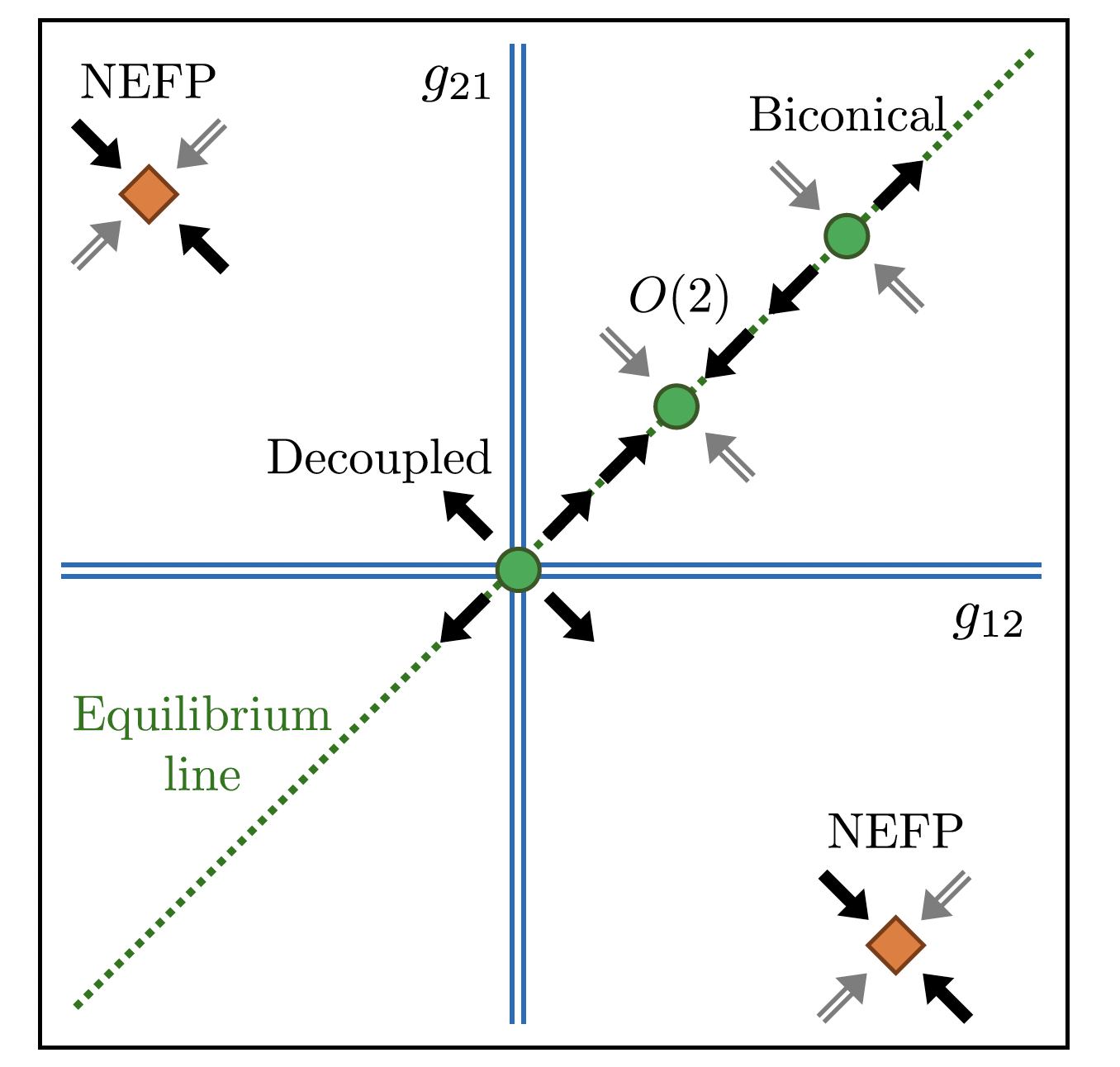
Figure 7: Portrait of the fixed points of two coupled critical Langevin models. When the microscopic couplings between the two order parameters are both positive, the RG flow is towards an attractive equilibrium $\mathrm{O}(2)$ theory. In contrast, when the flow is initiated with couplings of different signs, the flow is directed to one of two nonequilibrium fixed points (NEFP), which are multi-critical. Figure adapted from Ref. [623].

The key property of the dynamics of competing Ising order parameters with $g_{12},g_{21}\neq 0$ is that the condition for an effective equilibrium description is much more restrictive as compared to the case of a single order parameter. This opens up a route to escape effective thermalization. Indeed, obedience to the thermal symmetry of Sec. III.2 would require the dynamics to be governed by a single Hamiltonian, which can only occur when $g_{12}=g_{21}=g$. In this case, the equations of motion (78) can be derived from $H=H_{1}+H_{2}+\frac{g}{2}\int_{\mathbf{x}}\phi^{2}_{1}\phi^{2}_{2}$, and the steady-state distribution of the Langevin dynamics is a Gibbs state, $\rho\sim e^{-H/T}$. From an RG perspective, microscopic couplings can get renormalized in the flow to their fixed points. If the two coupling constants are both initialized with positive values [623], the RG flow will reach an equilibrium fixed point in the $\mathrm{O}(2)$ universality class. Fig. 7 shows in addition two unstable fixed points corresponding to the decoupled limit ($g_{12}=g_{21}=0$) and to a biconical fixed point [336].

The situation becomes richer when the two microscopic couplings, $g_{12}$ and $g_{21}$, are initialized with opposite signs, and thus realize a strongly nonreciprocal coupling [623]. As shown in Fig. 7, the RG flow is attracted towards a pair of nonequilibrium fixed points. These two fixed points have the same number of stable directions as the equilibrium fixed points, i.e., the same number of RG relevant parameters tuned to zero in order to approach criticality. Therefore, the RG flow can discriminate between the equilibrium and nonequilibrium fixed points using by the relative sign of the couplings as control knob.

An RG analysis to order $\mathcal{O}(\epsilon^{2})$ with $\epsilon=4-d$ the distance from the upper critical dimension $d_{u}=4$, reveals that the nonequilibrium fixed points are characterized by a discrete scale invariance of response and symmetric correlation functions reminiscent of fractals. This should be contrasted with the ubiquity of continuous scale invariance at equilibrium criticality and in most of the nonequilibrium critical points discussed so far in this review.

In addition, the nonequilibrium fixed points display an emergent effective temperature (cf. Sec. VIII.1), which scales in the infrared ($q\to 0$) as $T_{\textit{eff}}\propto q^{\eta-\eta^{\prime}}$. Here, $\eta$ and $\eta^{\prime}$ are the anomalous dimensions of fluctuations and dissipation, respectively. Their mismatch $\eta\neq\eta^{\prime}$ is a genuine signature of the system being out of equilibrium since this rules out the possibility of having a scale-independent temperature (cf. Sec. IV.2). We will see that this also occurs in the nonthermal quantum fixed point of Sec. XI.2; however, in that case the system retains quantum coherence, while in the case discussed in this section the system is fully classical. These exotic properties suggest that the multicriticality of driven open systems belongs to a new universality class and can become a frontier of exciting research in the years to come.

IX Slowly and rapidly driven open systems

So far, we have considered critical phenomena in nonequilibrium stationary states, where no explicit time dependence was involved. In this section, we address the question which novel universal phenomena emerge once such a time dependence is introduced. To this end, we will consider systems that exhibit a continuous phase transition and focus on the regimes of slow and fast drive. The limit of an undriven system with driving frequency $\Omega=0$ corresponds to thermodynamic equilibrium, and the limit of an infinitely rapidly driven and open system with $\Omega^{-1}=0$ is captured by a time-independent description in terms of a Lindblad equation. In the latter case, the combination of drive and dissipation creates a nonequilibrium situation as discussed in Sec. III, and critical behavior under these conditions has been studied in Sec. VIII.1.

Let us briefly anticipate the main results of the following discussion. The vicinities of both limiting points $\Omega=0$ and $\Omega^{-1}=0$ exhibit a similar phenomenology, characterized by a cutoff of the divergence of the correlation length upon approaching the transition point. However, this common trait is rooted in drastically different physical mechanisms, following from the fact that slow and fast drives exert low- and high-energy modifications, respectively. As a consequence, the critical exponents that determine the scaling of the correlation length at distances below the cutoff are unmodified in the slowly driven problem compared to the equilibrium case; yet the drive allows one to activate subleading scaling exponents [409, 350]. In contrast, the rapidly driven case exhibits an additional independent critical exponent [408, 410].

IX.1 Slowly driven systems: activating critical exponents

IX.1.1 Kibble-Zurek mechanism

The basic physics of a slowly driven system close to a second order finite-temperature or quantum phase transition is described by the Kibble-Zurek mechanism [326, 647, 476, 106]. It has been explored and validated in a broad spectrum of experiments, e.g., recently with a Rydberg quantum simulator [320]. Consider a slow ramp through the critical point as described by a time-dependent tuning parameter $g(t)=g_{0}-vt$, where for the initial value $g(0)=g_{0}$ the system is deep in the disordered phase and the critical point is reached for $g(t)=0$. Starting from $t=0$, the time evolution is adiabatic as long as the relaxation time $\tau$ of the system is small as compared to the rate of change of $g$ characterized by the time scale $t_{g}(t)=g(t)/\dot{g}(t)\approx g_{0}/v$. Close to the critical point, however, the relaxation time starts to diverge as $\tau\sim\xi^{z}$ where $\xi\sim g(t)^{-\nu}$ is the correlation length. Adiabaticity is broken when $\tau\sim g(t)^{-\nu z}\approx t_{g}(t)$, and the state of the system is frozen with correlations extending over a finite length scale $\xi$, which obeys a universal scaling form as a function of the drive velocity $v$ [476, 156, 45, 534]:

$$\xi\sim v^{-\frac{1}{z+1/\nu}}.$$ (80)

Notably, the Kibble-Zurek mechanism gives access to the dynamical exponent $z$, which is not available from the static correlation functions. However, as we discuss below, this is just the tip of the iceberg of a more general observation: By slowly driving the system in the vicinity of a phase transition, it is possible to access the full spectrum of critical exponents.

In fact, there are infinitely many universal numbers defining the exponent spectrum [112, 462, 566]. The customary exponents such as $\nu$ are associated with relevant couplings, and determine the leading scaling behavior. Exponents which are associated with irrelevant couplings provide only subleading corrections that are hard to resolve both in experiments [462] and in theory [194]. An exception are conformal field theories, where a relation between the scaling dimensions of operators and the energy spectrum has been established, making the subleading exponents amenable to exact numerics [357]. Nevertheless, as we demonstrate below, in slowly driven systems, these exponents become observable in the asymptotic scaling behavior of generic critical systems.

IX.1.2 Exact RG approach to slowly driven systems

As discussed above, in the adiabatic regime, the equilibration time scale is much shorter than the time scale of the drive. Time then only enters via the parameters characterizing the system. Therefore, the full set of adiabatic flow equations, which encodes the exact scaling dimensions of all couplings, is obtained from its undriven counterpart by promoting the static parameters to time-dependent ones, $k\partial_{k}\mathbf{g}(t)=\boldsymbol{\beta}(\mathbf{g}(t))$, where $k$ is the running momentum cutoff, and we bundle the couplings and the respective beta functions in vectors $\mathbf{g}=\mathbf{{g}}({t}\,)=({g}^{1}({t}\,),{g}^{2}({t}\,),\dotsc)$ and $\boldsymbol{\beta}$. We consider a linear drive, $\mathbf{g}(t)=\mathbf{g}_{0}+\mathbf{g}_{1}t$. A standard procedure [642, 566] yields the flow equations for dimensionless couplings $\mathbf{\hat{g}}_{0}$ and $\mathbf{\hat{g}}_{1}$. Crucially, time must be rescaled like any other parameter, leading to an additional contribution to the flow equations [409].

The phase transition is described by the Wilson-Fisher fixed point of the RG flow of dimensionless couplings. To find the critical exponents, the set of flow equations has to be linearized around this fixed point. We are interested in the vicinity of the usual equilibrium fixed point where $\mathbf{\hat{g}}_{1,*}=0$. In the adiabatic limit, the linearized flow equations for $\mathbf{\hat{g}}_{0}$ and $\mathbf{\hat{g}}_{1}$ decouple. The linearized flow of $\mathbf{\hat{g}}_{0}$ is described by a matrix $M$, whose eigenvalues determine the full spectrum of critical exponents. In contrast, the linearized flow of $\mathbf{\hat{g}}_{1}$ is determined by the matrix $M-z\mathbbm{1}$. This shows that only the eigenvalues of $M$ and $z$ itself determine the critical behavior of the adiabatic flow equations. That is, no new universal information is contained in the slowly driven system—it just probes the underlying equilibrium critical point, in analogy to the Kibble-Zurek result Eq. (80). However, the shift by $z$ can lead to additional relevant directions at the equilibrium Wilson-Fisher fixed point, whose physical consequences will be discussed below.

Let us consider a concrete example of a two-parameter RG flow obtained by truncating the infinite-dimensional matrix $M$ for an Ising magnet in zero external field. The eigenvalues $\theta_{i}$ of $M$ are then sorted by magnitude and labelled conventionally as $\theta_{1}\equiv-1/\nu$ and $\theta_{2}=\omega$, where $\nu>0$ is the relevant exponent describing the scaling of the correlation length according to $\xi\sim g^{\nu}$, and $\omega>0$ is the first irrelevant exponent [112]. Accordingly, the eigenvalues of $M-z\mathbbm{1}$ are shifted down to $-1/\nu-z$ and $\omega-z$. Typically, $z\approx 1$ for a linear dispersion or $z\approx 2$ for a quadratic dispersion or diffusion. In both cases, $z$ is larger in size than the typical value of $\omega$. For the example of the Ising model in three dimension, $1/\nu\approx 1.54$ and $\omega\approx 0.66$ [310], and the dynamical exponent $z\approx 2.013$ for model A dynamics [642, 566]. Therefore, due to the slow drive, there are two additional relevant directions. As we detail below, the first one leads to the Kibble-Zurek scaling in Eq. (80), and the second one to new scaling behavior.

IX.1.3 Observable consequences

When a system is tuned close to a continuous phase transition, the RG flow of dimensionless couplings will first approach the vicinity of the fixed point, before being pushed out of this critical domain along one of the relevant directions. In the above example of the two-parameter RG, there are three relevant directions at the Wilson-Fisher fixed point. For simplicity, let us assume that the matrix $M$ is diagonal, such that the couplings correspond to the eigendirections emanating from the fixed point. Then, $-1/\nu-z$ and $\omega-z$ are the exponents associated with the couplings $g_{1}^{1}$ and $g_{1}^{2}$, respectively. The exiting of the critical domain along either direction leads to the breaking of adiabaticity [350]. Therefore, the scale at which the critical domain is left determines the observable correlation length $\xi$ and will feature information on the respective exponents. The different exponents can be accessed, or activated, by approaching the phase boundary along different directions. This is illustrated in Fig. 8(a): Tuning the experimental knobs at velocity $v$ perpendicular to the phase border (blue arrow) corresponds to a ramping of the gap and is thus associated exclusively with $g_{1}^{1}$, i.e., $v\sim g_{1}^{1}$. In this case, adiabaticity is broken and the scaling of the observable correlation length is cut off at a scale $\xi$ that obeys the ‘traditional’ Kibble-Zurek scaling Eq. (80). In contrast, moving in parallel to the phase border is associated exclusively with time-dependent irrelevant couplings, which generically will have a component from the least irrelevant coupling $g_{1}^{2}$, i.e., $v\sim g_{1}^{2}$ now. Then, the correlation length scales as

$$\xi\sim v^{-\frac{1}{z-\omega}}.$$ (81)

That is, the irrelevant exponent $\omega$ is now activated in the leading asymptotic scaling behavior, and can thus be determined experimentally once $z$ is known.

A generic driving protocol is characterized by a velocity $\mathbf{v}=v\left(\cos(\theta),\sin(\theta)\right)$ in the two-dimensional phase diagram. In terms of the RG, this means that the couplings $g_{1}^{1}$ and $g_{1}^{2}$ get mixed—which one ‘wins’ in cutting off scaling depends on the drive angle $\theta$, and there is a crossover velocity $v_{*}$ separating two regimes of different asymptotic cutoff scaling, see Fig. 8(b). In a higher-dimensional phase diagram, more new scaling directions can be revealed by suitably chosen drives [409].

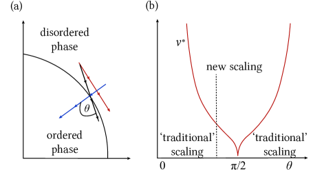
Figure 8: (a) Driving protocols: perpendicular (blue), parallel (red), and general (black) in a phase diagram with two experimental knobs (e.g. temperature and pressure). (b) Crossover velocity $v^{*}$ between different scaling regimes. For parallel drive $\theta=\pi/2$, the new scaling is observed even for small drive velocities.

These general findings are validated in the analytically solvable and experimentally relevant transverse XY model in Ref. [350]. In particular, it is shown that the driving protocol can be designed such that the excitation density of defects hosts the full sequence of exponents in its asymptotic scaling behavior.

IX.2 Rapidly driven systems: open Floquet criticality

We now turn to the opposite limit and focus on periodically driven or Floquet systems with fast driving. For closed and interacting systems, periodic driving generically leads to heating. Even though the heating time scale is exponentially large in the drive frequency, so that a quasi-stationary prethermal state can emerge on intermediate time scales, such systems will eventually heat up to infinite temperature [3, 428, 347, 2, 183, 426, 272, 531]. In contrast, coupling a Floquet system to a heat bath can stabilize the entropy density at finite values, and at asymptotically long times, observables become stationary up to a periodic time dependence with frequency $\Omega$ imposed by the drive—the system synchronizes to the latter. Here, we focus on such open Floquet steady states. The nature of symmetry-breaking phase transitions in rapidly driven, open systems has been investigated in Ref. [408]. Technically, this amounts to the question of how to renormalize an open Floquet system [410]. Prior RG-based work has addressed this question in the slowly-driven limit [157, 444, 193], and numerical studies have focused on intermediate driving frequencies [334, 210, 95, 382]. Here, we concentrate on the effect of fast, but not infinitely fast driving.

IX.2.1 Basic physical picture

A key result of this analysis is that rapid weak drive prevents the correlation length from diverging, in some phenomenological similarity to the Kibble-Zurek scenario. Pristine criticality is thus absent and restored only in the limit of infinitely rapid drive discussed in Sec. VIII.1. At first sight, such a drastic modification of the nature of the phase transition might be unexpected—the drive provides a fast scale $\Omega$, which should not affect the long-wavelength critical properties. However, in the driven system energy is conserved only $\text{mod}(\Omega)$, and the notion of ‘high’ and ‘low’ energy is thus not well defined. Based on this fact the system evades the common reasoning, as will be shown below. A picture that captures the essence of the mechanism is instead obtained based on the synchronization of the relevant spectral gap $r_{d}$ (cf. Sec. IV.2.1; we denote it as in Eq. (38), since we will specialize to this model below) to the drive,

$$r_{d}(t)=r_{d,0}+\sum_{n\neq 0}r_{d,n}e^{-in\Omega t}.$$ (82)

Even when the static system is critical for $r_{d,0}\rightarrow 0$, the synchronized mass still oscillates and is dragged periodically across the phase transition. This leads to a blurring of the phase boundary. In particular, the divergence of the correlation length is cut off for any $\Omega<\infty$. Only in the limit of infinitely fast driving, the rotating wave approximation, in which all contributions with $n\neq 0$ are set to zero, becomes exact. Then, criticality is restored.

IX.2.2 Keldysh-Floquet model

Our microscopic starting point is a generalization of the model for driven open Bose-Einstein condensation from Sec. II, where now we assume the Hamiltonian to be periodically time dependent, $\hat{H}(t+2\pi/\Omega)=\hat{H}(t)$. As discussed in Sec. IV.3.2, close to the condensation transition, a semiclassical description applies. The corresponding Keldysh action is given in Eq. (38) but with time-dependent coupling constants. Anticipating full decoherence in the critical semiclassical model, all couplings can be approximated as being purely imaginary [410].

Key structures governing the behavior of the open Floquet system close to criticality are contained in the single-particle Green’s function $G(t,t^{\prime})$ which, for explicitly broken continuous time-translation symmetry, depends on both $t$ and $t^{\prime}$. It is convenient to switch to the Wigner representation [27, 619, 557, 576, 223],

$$G\!\left(t+\tfrac{\tau}{2},t-\tfrac{\tau}{2}\right)=\sum_{n}\int\frac{d\omega}{2\pi}e^{-i(n\Omega t+\omega\tau)}G_{n}(\omega),$$ (83)

where the discrete time translation invariance is encoded in a Fourier series with fundamental frequency $\Omega$, while the dependence on the relative time $\tau$ is represented through a Fourier transform as familiar from undriven stationary states. Corrections to the rotating wave approximation can be obtained through an expansion of $G_{n}(\omega)$ in powers of $r_{d,n\neq 0}/\Omega$. As illustrated in Fig. 9(a), the poles of the retarded Wigner Green’s function $G^{R}_{n}(\omega)$ form lines in the complex plane, corresponding to different Floquet-Brillouin zones that are separated along the real axis by integer multiples of $\Omega$. Under the assumption of purely imaginary couplings, these lines are parallel to the imaginary axis. Importantly, all lines of poles become critical simultaneously as $r_{d,0}\to 0$.

Figure 9: (a) The poles of the retarded Wigner Green’s function are organized in lines (shown in red; parallel to the imaginary axis for the purely dissipative open Floquet problem considered here) and separated along the real axis by the drive frequency $\Omega$. The origin of the real axis is arbitrary, whereas the distance from the origin along the imaginary axis $r_{d,0}$ denotes the distance from the phase transition point. Renormalization up to a scale $k$ corresponds to integrating out modes along the lines of poles, indicated by blue shading. (b) RG flow of dimensionless couplings. The horizontal plane, spanned by the mass $\hat{r}_{d,0}$ and the interaction strength $\hat{u}_{d,0}$, hosts the usual Wilson-Fisher fixed point (red dot) with one relevant direction. The fast drive provides an additional new relevant direction $\hat{x}\sim\Omega^{-1}$.

IX.2.3 Renormalization of the open Floquet problem

Renormalizing the open Floquet problem corresponds to integrating out modes along the lines of poles in the complex plane, as indicated by the blue shading in Fig. 9. All lines of poles contribute with the same degree of divergence, even though for weak driving with $r_{d,n\neq 0}/\Omega\ll 1$, higher Floquet-Brillouin zones are suppressed. In an $\epsilon=4-d$-expansion close to the upper critical dimension $d_{u}=4$, the flow equations for dimensionless variables to order $O(\epsilon r_{d,n\neq 0}/\Omega)$ read

$$\begin{split}k\partial_{k}\hat{u}_{d,0}&=-\epsilon\hat{u}_{d,0}+\frac{10S_{d}}{\left|1+\hat{r}_{d,0}\right|\left(1+\hat{r}_{d,0}\right)}\hat{u}_{d,0}\left(\hat{u}_{d,0}+\hat{x}\right),\\ k\partial_{k}\hat{r}_{d,0}&=-2\hat{r}_{d,0}-\frac{4S_{d}}{\left|1+\hat{r}_{d,0}\right|}\left(\hat{u}_{d,0}+\hat{x}\right),\\ k\partial_{k}\hat{x}&=-\epsilon\hat{x},\end{split}$$ (84)

with ${S_{d}=2\pi^{d/2}/[(d/2-1)!(2\pi)^{d}]}$ and dimensionless couplings $\hat{r}_{d,0}=k^{-2}\frac{r_{d,0}}{K_{d,0}}$ and $\hat{u}_{d,0}=k^{d-4}\frac{\gamma u_{d,0}}{4K_{d,0}^{2}}$. The effect of higher harmonics with $n\neq 0$ is subsumed in a new coupling $\hat{x}$. It can be shown that this coupling receives no loop corrections at order $O(\epsilon r_{d,n\neq 0}/\Omega)$, so it only shows dimensional running, and the set of flow equations is closed [408].

The flow equations (84) generalize those of time translation invariant $\mathrm{U}(1)$ systems. Indeed, as shown in Fig. 9(b), the standard Wilson-Fisher fixed point emerges when $\hat{x}=0$. The analysis shows that the periodic drive gives rise to a new relevant coupling. In the absence of continuous time translation invariance, the critical point is thus bicritical: Fine-tuning of two parameters is necessary to reach it, and to reveal its critical scaling properties. In an experiment, one will tune across the symmetry breaking phase transition at finite $\hat{x}\sim\Omega^{-1}$. Then, the additional relevant direction provides a finite correlation length. Consequently, this constitutes a symmetry-breaking phase transition without asymptotic criticality.

This finding can be interpreted within the framework of fluctuation-induced first order transitions [138, 268, 202, 442]: The interplay of several modes that simultaneously become critical changes the phase transition from a second to a first order one. This occurs without an explicit symmetry breaking as is usually present in first order phase transitions with a critical endpoint of higher symmetry. While in the traditional instances of this scenario, the gapless modes are realized by a critical mode coupled to Goldstone or gauge modes, here they are realized by the poles of the different Floquet-Brillouin zones, all reaching criticality jointly.

As usual, the critical exponents can be obtained from a linear stability analysis of the RG flow equations close to the Wilson-Fisher fixed point [408, 410],

$$-1/\nu=-2+2\epsilon/5,\quad-\omega=\epsilon,\quad-1/\nu_{d}=-\epsilon.$$ (85)

The first two exponents are known and unmodified as compared to both the undriven problem and the infinitely rapidly driven system, which shares the static exponents with the equilibrium situation as discussed in Sec. VIII.1. In contrast, the exponent $\nu_{d}$ is new, adding an independent relevant direction to the Wilson-Fisher fixed point. The discussion can now be led in analogy to Sec. IX.1: In the presence of two relevant couplings, the observed scaling of the correlation length depends on the direction under which the fixed point is approached. For example, when the system is infinitely rapidly driven, $\hat{x}=0$, the correlation length diverges as $\xi\sim r_{d,0}^{-\nu}$. However, crossing the phase boundary with $\hat{x}\neq 0$, the correlation length never diverges due to the repulsive direction, and $\xi$ saturates to a finite value that scales as $\xi\sim x^{-\nu_{d}}$ with the distance from the fixed point. In particular, this implies that the new critical exponent $\nu_{d}$ can be observed by varying $\Omega$. This is a key quantitative and universal prediction of this analysis.

IX.2.4 Relation to the slowly driven limit

The above discussion shows that the mechanism established here for a rapid drive is distinct from the slowly driven Kibble-Zurek scenario investigated in Sec. IX.1—despite the phenomenological similarity that close to the limits of undriven and infinitely rapidly driven systems, scaling is cut off. In RG language, this is due to the emergence of new relevant directions at the respective fixed points. But the difference is also transparent in this language: As we have discussed, in the Kibble-Zurek scenario, the drive provides information on the underlying equilibrium critical point via the set of equilibrium critical exponents, because the new relevant directions just host information that is already encoded in the equilibrium fixed point. Instead, for rapid drive we obtain a new independent exponent (actually, more than one, see Ref. [410]). This is rationalized by the fact that in the former case, we deal with an infrared modification of the critical physics: A slow driving scale is introduced, so slow that the periodic functions in Eq. (82) can be expanded in powers of $\Omega$ and the periodicity is never probed on the accessible time scales. Conversely, in the latter case, the modification is in the ultraviolet: A fast driving scale is introduced, and the periodicity is crucial. Another way of seeing this is the presence of the additional mass scales in Eq. (82), connecting back to the intuitive picture of synchronized mass oscillations provided at the beginning of this section. It is a basic but also fundamental insight of RG theory that it is such ultraviolet scales that can modify and add critical exponents to the observable phenomenology [237].

X Nonequilibrium first order phase transitions

First order phase transitions appear in many important physical scenarios [67], including every day’s boiling of water and hysteresis in ferromagnetic materials, and are characterized by a discontinuous jump of static, thermodynamic observables. Due to the discontinuous behavior, i.e., due to the absence of scaling in static observables, first order phase transitions are often associated with an absence of universal behavior. This is misleading, since first order phase transitions display universal behavior in a broader sense: one can easily identify recurring patterns that are shared ubiquitously amongst systems undergoing a first order phase transition.

The hallmark of any first order phase transition is the coexistence of two macroscopically distinguishable, thermodynamic phases. In thermal equilibrium, this coexistence corresponds to a bistability in the system’s free energy, which persists under coarse graining up to the largest distances. Both the presence of a bistability and the distinguishability of the two phases imply that the correlation length remains finite and does not diverge when the transition point is crossed.

A nondiverging correlation length gives rise to a peculiar phenomenology, including structurally distinct dynamics that appear on different length scales. This in turn leads to a variety of experimentally observable phenomena such as scale invariant excitation avalanches [538] (cf. crackling noise [537]) and intermittency between two phases [464, 35]. The general phenomenology of first order transitions is reviewed below. This is followed by a discussion of how the transitions may be enriched if the dynamics are placed out of thermal equilibrium [368, 416, 390, 208, 610].

X.1 General phenomenology of first order phase transitions

We provide a brief summary of the phenomenology of first order phase transitions in thermal equilibrium from the perspective of effective field theory. For an in-depth overview, we refer to the literature, e.g., the reviews [65, 620, 61]. For an elementary model, consider a real scalar order parameter field $\phi(t,{\bf x})$ governed by a Langevin equation of the form (we set $\phi\equiv\phi(t,\mathbf{x}),\eta\equiv\eta(t,\mathbf{x}))$

$$\partial_{t}\phi=D\nabla^{2}\phi-V^{\prime}(\phi)+\eta,$$ (86)

where $V^{\prime}(\phi)=dV(\phi)/d\phi$, and $\eta$ is a Gaussian white noise with average $\langle\eta(t,\mathbf{x})\rangle=0$ and variance $\langle\eta(t,{\bf x})\eta(t^{\prime},{\bf x}^{\prime})\rangle=2T\delta(t-t^{\prime})\delta({\bf x}-{\bf x}^{\prime})$. This imprints thermal fluctuations with temperature $T$. In order to realize a bistability, the potential $V(\phi)$ must take the form of a double- or multi-well. For concreteness, consider a tilted $\phi^{4}$-potential $V(\phi)=\frac{u_{2}}{2}\phi^{2}+\frac{u_{4}}{4}\phi^{4}-\frac{2\alpha\sqrt{u_{2}u_{4}}}{3}\phi^{3}$, where the dimensionless parameter $\alpha$ tunes the strength of the tilt. For $u_{2},u_{4}>0$ and $\alpha>1$ the potential has two stable field configurations at $\phi=0$ and $\phi=\varphi_{f}\equiv\sqrt{u_{2}/u_{4}}(\alpha+\sqrt{\alpha^{2}-1})$ and a separatrix at $\phi=\sqrt{u_{2}/u_{4}}(\alpha-\sqrt{\alpha^{2}-1})$. The solution $\phi=0$ is favored, i.e., is the global minimum, for $\alpha\leq\alpha_{c}=3/\sqrt{8}$. We introduce the order parameter $\varphi$ as the spatial average $\varphi=\frac{1}{V}\int_{V}d\mathbf{x}\,\langle\phi\rangle$ over the system volume $V$.

Mean-field theory predicts a first order phase transition and coexistence of the solutions $\varphi=0$ and $\varphi=\varphi_{f}$ at $\alpha=\alpha_{c}$, when the global minimum of $V$ jumps from $\phi=0$ ($\alpha<\alpha_{c}$) to $\phi=\varphi_{f}$ ($\alpha>\alpha_{c})$. In the dynamics, $\phi$ undergoes strong fluctuations in the vicinity of this point, performing local noise-induced transitions between the two solutions. One distinguishes three different dynamical regimes, according to the typical length scale on which they are observed. The relevant, emergent length scale is the so-called droplet length $\xi_{D}$. It arises from the competition between noise and diffusion [355, 354] in an instanton-type calculus.

(i) Short distance fluctuations: On short distances $|\mathbf{x}|\ll\xi_{D}$, the field $\phi$ performs fast (on time scales smaller than $1/T$ ) but small fluctuations around one potential minimum. They are driven by the competition between thermal noise $\sim T$ and diffusion $\sim D\nabla^{2}$. Diffusion favors smooth configurations of $\phi$ in space and suppresses noise-induced short-distance fluctuations. In particular, it prevents local fluctuations from reaching across the potential barrier. Short distance fluctuations are thus ‘blind’ to the double-well structure and only explore the vicinity of one of the potential minima. This leads to a smooth renormalization of the potential $V$ [61, 497, 503].

(ii) Droplet nucleation: On sufficiently large distances $|\mathbf{x}|\sim\xi_{D}$, thermal fluctuations may induce a spontaneous, local but smoothly varying transition of the field $\phi$ from one minimum to the other, $0\leftrightarrow\varphi_{f}$. This process is known as droplet nucleation [354, 186]. The spontaneously generated droplet has a finite volume. Its size is determined by the competition between diffusion, preferring extended, smooth configurations, and the fluctuation strength, preferring local excitations. The droplet is bounded by a sharp domain wall, which interpolates between the two different phases, e.g., between $\phi=0$ inside the droplet and $\phi=\varphi_{f}$ outside of it. The nucleation corresponds to the formation of an instanton configuration of the field $\phi$ [356, 137], as it is known from the theory of the false vacuum. It describes rare noise activation processes, which lead to large fluctuations of the field $\phi$ at the droplet length scale $\xi_{D}$. These rare fluctuations exceed the typical statistical fluctuations by far (cf. the formation of steam bubbles in boiling water). This behavior also manifests in the RG flow of the theory discussed below.

(iii) Domain wall motion: After nucleation, droplets either grow or decay. On length scales much larger than the droplet scale $|\mathbf{x}|\gg\xi_{D}$, the direction of growth is governed by the interface between the two phases, i.e., by the motion of domain walls. On average, the domain wall motion favors to decrease the potential energy. Hence, droplets grow (shrink) if they correspond to the global (local) minimum of the potential. This determines the thermodynamic phase of the system. At the transition, the energy difference between both phases, and thus the average domain wall velocity, vanishes, leading to slow phase ordering kinetics [211, 65].

X.2 First order phase transitions out of equilibrium

How is the picture of first order phase transitions modified out of equilibrium? On a formal level, i.e., on the level of the Langevin equation, the modification is similar to the case of second order phase transitions. In order to discuss the possible scenarios, consider an $N$-component order parameter field $\phi_{a}\equiv\phi_{a}(t,\mathbf{x})$, $a=1,\dotsc,N$, which obeys the Langevin equation

$$\partial_{t}\phi_{a}=D\nabla^{2}\phi_{a}+F_{a}(\boldsymbol{\phi})+\eta_{a},$$ (87)

where $F_{a}(\boldsymbol{\phi})$ is the field-dependent force and $\langle\eta_{a}\eta_{b}\rangle=\chi_{ab}(\boldsymbol{\phi})\delta(t-t^{\prime})\delta(\mathbf{x}-\mathbf{x}^{\prime})$ is a Gaussian white noise, which imposes local field fluctuations with strength $\chi_{ab}(\boldsymbol{\phi})$. In thermal equilibrium, two conditions are simultaneously met [286, 541]: (i) the deterministic force derives from a potential form $V$, i.e., $F_{a}(\boldsymbol{\phi})\equiv-\partial_{\phi_{a}}V(\boldsymbol{\phi})$, and (ii) a flat noise spectrum $\chi_{ab}(\boldsymbol{\phi})\equiv\delta_{a,b}T$ ensures a conventional fluctuation-dissipation relation. Out of equilibrium, one generally distinguishes the following two scenarios:

(i) Absence of a potential form: One way to break detailed balance, and hence enforce nonequilibrium conditions, is the absence of a potential form for the force $F_{a}(\boldsymbol{\phi})\neq-\partial_{\phi_{a}}V(\boldsymbol{\phi})$. Bistability at a first order phase transition requires two (or more) field configurations $\boldsymbol{\phi}_{1,2}$ to be solutions of $\mathbf{F}(\boldsymbol{\phi}_{1,2})=0$. However, the transition cannot be derived from an extremization principle, i.e., from the minimization of a global free energy. Instead, the system will evolve into a flux equilibrium where the sum of all possible paths connecting $\boldsymbol{\phi}_{1}\leftrightarrow\boldsymbol{\phi}_{2}$ is balanced [247, 246]. One example discussed in Sec. VII.4.3 is vortex turbulence, which arises in a compact, single-component KPZ equation. A second important example are nonreciprocal systems [208, 610, 222, 633], where first order phase transitions correspond to an exceptional point in the system’s linear stability matrix $A_{ab}\equiv\partial_{\phi_{b}}F_{a}(\boldsymbol{\phi})|_{\boldsymbol{\phi}=0}$. Such situations describe, e.g., flocking and synchronization phenomena in active matter or non-Hermitian systems [208, 610, 271, 633].

(ii) Absorbing states: Another way to impose nonequilibrium conditions is via a state-dependent noise kernel $\chi(\boldsymbol{\phi})$. Under certain conditions, such a noise kernel imposes the breaking of detailed balance akin to absorbing state phase transitions and directed percolation in Sec. V. For simplicity, we discuss this case for a scalar field $\phi$. The state-dependence of $\chi$ implies that the noise is biased. It induces strong fluctuations of the field $\phi$ when $\chi(\phi)$ is large and weak fluctuations when $\chi(\phi)$ is small. This may influence the stationary solution for the optimal field configuration. Consider for instance two degenerate minima of the potential $V(\phi_{1})=V(\phi_{2})$. Then of the two, the configuration with smaller noise is the more stable one. For the case of state-dependent fluctuations, one can define a modified free energy landscape $W(\phi)$ if and only if $W$ solves the equation $\partial_{\phi}W(\phi)=-F(\phi)/\chi(\phi)$ for the entire configuration space of $\phi$. If such a solution exists, then the system fulfills an effective detailed balance with respect to $W(\phi)$. If no such solution exists, then detailed balance is truly broken. This is the case when $\chi(\phi)^{-1}$ is singular for some field configuration $\phi^{\prime}$, e.g., when $\chi(\phi^{\prime})=0$. In particular, this is the case when a bistability occurs between an active and an absorbing phase, i.e., a dark state for which $\chi(\phi)=0$ at one of the bistable states [397, 497]. A setup where this scenario occurs has been introduced for ultracold Rydberg gases in the facilitation regime discussed in Sec. V.2. Here, the quantum mechanical origin of the facilitation mechanism introduces a bistability between a dark state and an active state at high atom density. This scenario has been highlighted in Ref. [398, 92] and is reviewed in Sec. X.3 below.

X.3 Dark state bistability

For a bistability separating an ordered phase from a dark state, the first order phase transition is significantly modified. As discussed in Sec. V.2, a dark state $\hat{\rho}_{D}=|D\rangle\langle D|$ is a pure quantum state, in which the order parameter $\varphi$ and its fluctuations vanish (cf. Appendix D). In contrast, the ordered (active) phase yields a nonzero value for the order parameter and its fluctuations, and resides in a mixed state.

A first order phase transition between an active and a dark state thus readily dictates a set of modifications:

(1) Coexistence: The dark state has a local product state structure, e.g., ${\hat{\rho}_{D}=\prod_{l}|\downarrow\rangle\langle\downarrow|_{l}}$ for Rydberg atoms (cf. Sec. V.1). Coexistence between an active phase and a dark state implies that the system hosts an extensive volume $V_{D}$ which is in the dark state. Inside this volume, the order parameter and thus the fluctuations vanish. Hence, the state of the total system is well approximated by a product $\hat{\rho}=(\hat{\rho}_{\text{active}})_{\bar{V}_{D}}\otimes(\hat{\rho}_{D})_{V_{D}}$ between a pure state $\hat{\rho}_{D}$, constrained to the volume $V_{D}$, and a mixed state $\hat{\rho}_{\text{active}}$ on its complement $\bar{V}_{D}$.

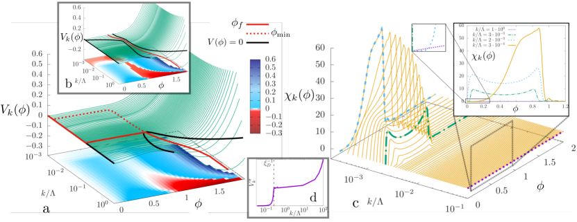
Figure 10: RG flow of the potential $V_{k}$ and noise kernel $\chi_{k}$ at a first order phase transition in $d=3$ dimensions. The microscopic model is given by the Langevin equation (88) with initial conditions $V_{\Lambda}=\tfrac{1}{2}\phi^{2}+\tfrac{1}{4}\phi^{4}-\tfrac{2\alpha}{3}\phi^{3}$ and noise kernel $\chi_{\Lambda}=\tfrac{1}{10}\phi$. (a) $\alpha=3.48$, (b) and (c) $\alpha=3.5$. The flow at large momenta $k\sim\Lambda$ yields small corrections to the potential landscape: The minimum at $\phi>0$ moves slightly and becomes nearly degenerate to the dark state at $\phi=0$ in (a) and (b). (d) The flow of $V^{\prime\prime}(0)$ provides an estimate for the change of the potential toward a convex function. At the droplet scale $k_{D}=\xi_{D}^{-1}$, it undergoes a sudden, sharp drop. (c) At this scale $\chi_{k}$ increases by three orders of magnitude. It assumes a bimodal form indicating large droplet fluctuations. At the largest distances fluctuations are suppressed again, confirmed by the inset. Figure adapted from Ref. [497].

(2) Droplet nucleation: Fluctuations are absent in the dark state volume $V_{D}$. This prohibits noise activation from the dark state to the active phase. Droplets appear exclusively in the active phase volume $\bar{V}_{D}$, This leads to a unidirectional fluctuation pattern where local noise-induced transitions can only follow the path $\hat{\rho}_{\text{active}}\to\hat{\rho}_{D}$. Hence, one finds a maximally extended hysteresis loop: once the global dark state has been reached, there is no return to the active phase.

(3) Domain wall motion: The domain walls experience a similar unidirectional fluctuation pattern. The presence (absence) of fluctuations in the active (inactive) phase makes the domain walls favor the dark state and extend the volume $\bar{V}_{D}$. This bias needs to be compensated by a nonzero difference in the potential energy. Hence, the noise $\chi$ and the potential $V$ can no longer be treated independently.

Items (1)–(3) are relevant for the field theory approach to a first order dark state phase transition. In particular, the interplay between the potential and the noise for both the domain wall motion and the droplet formation requires a treatment of the potential and the fluctuations on equal footing, i.e., an RG-approach in the Keldysh field integral framework. This approach provides an unambiguous identification of the three dynamical regimes (i)–(iii) in Sec. X.1, and their modifications (1)–(3) at a dark state transition [497].

X.4 Field theory of first order dark state phase transitions

The dynamics at a dark state bistability with a scalar order parameter field $\phi\equiv\phi(t,\mathbf{x})$ and with a potential form can be examined in a Langevin framework as in Eq. (86). The dark state at $\phi=0$ is implemented by a modified noise kernel [497, 109] as in Eq. (87):

$$\partial_{t}\phi=D\nabla^{2}\phi-V^{\prime}(\phi)+\eta.$$ (88)

Here $V$ is as defined above and the Gaussian noise $\eta$ has zero mean and variance $\langle\eta(t,{\bf x})\eta(t^{\prime},{\bf x}^{\prime})\rangle=\chi(\phi)\delta(t-t^{\prime})\delta(\mathbf{x}-\mathbf{x}^{\prime})$. The noise kernel $\chi(\phi)$ is a positive, continuous function of $\phi$, which vanishes in the dark state, $\chi(\phi=0)=0$. For concreteness, one may assume $\chi(\phi)=\kappa\phi$ for some $\kappa,\phi>0$. This form of $\chi$ and $V$ is inspired by the Rydberg setup discussed in Sec. V.2, which yields Eq. (88) in the high density regime [398, 92].

The Langevin equation (88) describes the evolution of the field $\phi$ on short distances. A conventional, perturbative RG approach yielding the effective field theory on large distances is not applicable at a first order phase transition, due to the presence of a length scale and the absence of universal scaling behavior. Nonperturbative approaches based on the functional RG [612, 109, 108, 180] are more promising, and have been successfully applied [497, 61]. For a nonequilibrium bistability as described by Eq. (88), a convenient implementation of the functional RG is performed in momentum space. The general formulation for the RG transformations in the nonequilibrium Keldysh (or Martin-Siggia-Rose) framework can be found, e.g., in Refs. [541, 109, 497]. At RG scale $k$, it yields an effective theory for the field $\phi$ defined over momenta $q<k$ by integrating out short distance fluctuations with momenta $q>k$.

The first order transition can be approached in a Langevin truncation, which was introduced in Ref. [497]. In this framework, each RG transformation, i.e., each integration over short distance fluctuations, modifies the potential $V$ and the noise kernel $\chi$. At RG scale $k$, the dynamics are described by the Langevin equation (88) with

$$V\to V_{k},\ \chi\to\chi_{k}.$$ (89)

The potential $V_{k}$ and the noise kernel $\chi_{k}$ transform under each RG step. A truncation of this form ensures that the evolution of the distribution function of the field $\phi$ at each momentum scale $k$ follows a regular Fokker-Planck equation, and thus remains a well-defined, nonnegative probability distribution under coarse graining. In general, one might also include a scale-dependent wave function renormalization, $\sim Z_{k}\partial_{t}\phi$, and diffusion $\sim D_{k}\nabla^{2}\phi$, but their evolution is expected to be negligible due to the finite correlation length (verified in Ref. [497] for Eq. (88)).

The Keldysh action for the effective Langevin equation is

$$S_{k}=\int_{t,{\bf x}}\phi_{q}\left[\left(\partial_{t}-D\nabla^{2}\right)\phi_{c}+V^{\prime}_{k}(\phi_{c})-\chi_{k}(\phi_{c})\phi_{q}\right].$$ (90)

This imposes a polynomial dependence on the quantum (response) field $\phi_{q}$, but leaves the functional dependence on the classical field $\phi_{c}$ general. As mentioned above, such a truncation ensures that the theory at each RG step can be mapped to an appropriate Langevin or Fokker-Planck equation. Loosening this restriction, one may allow a more general dependence on the $\phi_{q}$-fields as, e.g., discussed in Refs. [109, 108]. For the bistability in Eq. (88), such modifications remain, however, negligibly small [497]. One may expect this behavior to be general for semiclassical theories whose distribution function is governed by a Fokker-Planck equation at all relevant scales.

For the Langevin truncation, the RG equations for the (unrescaled) potential and noise vertex are [497, 108] (setting the diffusion constant $D=1$ and dropping the field dependence in the argument)

$$\begin{split}\partial_{k}V^{(1)}_{k}&=U_{k,d}V_{k}^{(3)},\\ \partial_{k}\chi_{k}&=U_{k,d}\left(\chi^{(2)}_{k}-4\frac{\chi^{(1)}_{k}V^{(3)}_{k}}{\left(k^{2}+V^{(2)}_{k}\right)}+\frac{\chi_{k}(V^{(3)}_{k})^{2}}{2\left(k^{2}+V^{(2)}_{k}\right)^{2}}\right),\end{split}$$ (91)

with $U_{k,d}=-k^{d+1}\chi_{k}\left[2^{d-1}\pi^{\frac{d}{2}}\Gamma\left(\frac{d}{2}\right)d\left(k^{2}+V^{(2)}_{k}\right)^{2}\right]^{-1}$. At a first order phase transition, the fields $\phi_{c},\phi_{q}$ do not obey canonical power counting. Thus a polynomial expansion of the potential and the noise kernel cannot be justified. It is then necessary to keep the general functional form of $V_{k}$ and $\chi_{k}$, and to solve the flow equations numerically.

X.5 Renormalization group flow

The phenomenology of the first order phase transition, including the modifications from the dark state, is reflected in the numerical solution of the flow equations (91) for the bistability equation (88) [497]. Close to a first order transition, the RG flow of the potential $V_{k}$ and noise $\chi_{k}$ reveal regimes (i)–(iii) from Sec. X.1:

(i) At short distances, i.e., at large momenta $k\gg\xi_{D}^{-1}$, where $k=\Lambda\gg\xi_{D}^{-1}$ is the UV cutoff, the potential $V_{k}$ is weakly renormalized (flattened) due to integrating over short wavelength fluctuations (see initial stage of the RG flow for $k/\Lambda\geq 0.1$ in Fig. 10).

(ii) At a sharp momentum scale $k_{D}\Lambda=\xi_{D}^{-1}\Lambda\approx 0.1$, both the potential $V_{k}$ and the noise kernel $\chi_{k}$ experience a sudden, strong renormalization (witnessed by $V_{k}^{\prime\prime}$ in Fig. 10(d)). The potential approaches a nearly degenerate bistability, $V_{k}(\phi=0)\sim V_{k}(\phi=\varphi_{f})$. The noise kernel $\chi_{k}$ assumes a bimodal structure with peaks at $\phi=0,\varphi_{f}$, see Fig. 10(c). This indicates strong fluctuations of the field between the two minima, i.e., the onset of droplet nucleation at the scale $k_{D}=\xi_{D}^{-1}$.

(iii) At momenta $k\ll k_{D}$, on distances much larger than the droplet scale $\xi_{D}$, the noise kernel $\chi_{k}$ becomes flat $\chi_{k}(\phi)\approx 0$ for $\phi\in[0,\varphi_{f})$. The corresponding Langevin equation Eq. (88) is noiseless and describes deterministic domain wall motion. Asymptotically ($k\to 0$) the potential assumes a linear form $V_{k}(\phi)\sim\phi$ and vanishes at the bistability $V_{k}(\phi)=\chi_{k}(\phi)=0$ for $0<\phi<\varphi_{f}$.

This reconciles the field theory with the general phenomenology of first order phase transitions, and in particular with a dark state transition. Phase coexistence between a dark state and an active state requires both the deterministic dynamics generated by $V_{k}$ and the noise $\sim\chi_{k}$ to vanish. The renormalization group flow of the noise kernel $\chi_{k}$ and the interplay between $V_{k}$ and $\chi_{k}$ is crucial to resolve this behavior.

Whether first order dark state phase transitions can be observed in driven quantum systems is a topic of ongoing research. Several possible scenarios have been proposed [186], ranging from Rydberg atoms in the facilitation regime [397, 497, 92, 594, 368, 309], to cellular automata [230], or between two different dark states [118]. However, first order phase transitions are often unstable against fluctuations in low dimensions [497, 385, 284]. Thus, they are restricted to higher dimensions $d\geq 2$, where numerical simulations of quantum dynamics are challenging. This is at the moment a major obstacle in identifying first order dark state transitions.

XI Quantum criticality in driven open systems

The previous sections have covered driven open quantum systems whose scaling descriptions fall into extensions of thermal universality classes, or constitute novel nonequilibrium fixed points per se. In each of the cases presented, the microscopic quantum nature of the problem is levelled out on long wavelengths and becomes inconsequential for the effective field theory description. Here, instead, we will cover two instances of the quantum scaling limit mentioned in Sec. IV.3.2, marking the commencement of the third and last thematic part of this review (cf. Tab. 1) . We will focus on noise-driven one-dimensional (1D) bosonic systems whose quantum features can persist over long length and time scales. Specifically, we will consider a Luttinger liquid driven by $1/f$ noise (Sec. XI.1), and a driven open condensate subjected to diffusion noise (Sec. XI.2), i.e., Markovian noise whose variance scale quadratically with momentum. Both models illustrate how the formation of nonequilibrium quantum critical states is determined by the interplay between dissipation and nonlinearities. In the former case (XI.1), scaling manifests in nonuniversal exponents controlled by the noise strength, while in the latter case (XI.2), scaling is governed by a quantum fixed point without classical counterpart, leading to universal scaling exponents that define a novel universality class.

XI.1 Quantum critical scaling of noise-driven Luttinger liquids

We follow Refs. [152, 153, 154] and consider a 1D bosonic wire, described as a Luttinger liquid with periodic potential of strength $g$, and driven by a noise field $f(t)$ that couples to fluctuations of the density. The Hamiltonian reads

$$\hat{H}(t)=\int\frac{dx}{u}\left[K\left(u\pi\partial_{x}\hat{\theta}(x)\right)^{2}+\frac{1}{K}\left(u\partial_{x}\hat{\phi}(x)\right)^{2}\right.\\ \left.\vphantom{\left(u\partial_{x}\hat{\phi}(x)\right)^{2}}-g\cos\!\left(2\hat{\phi}(x)\right)\right]-\frac{1}{\pi}\int\frac{dx}{u}f(t)\partial_{x}\hat{\phi}(x)+H_{\mathrm{bath}}(\hat{\phi}(x)),$$ (92)

where $\hat{\theta}(x)$ and $\hat{\phi}(x)$ are Hermitian operators encoding, respectively, the phase of the bosons and their long-wavelength density fluctuations, satisfying canonical commutation relations [225]. $K$ is the Luttinger parameter, and $u$ is the speed of sound. In Eq. (92), we have included the Hamiltonian of a zero-temperature Ohmic bath, $H_{\mathrm{bath}}(\small{\hat{\phi}(x)})$, linearly coupled to $\partial_{x}\hat{\phi}(x)$ and with friction $\eta$, which serves to damp heating induced by the noise term $f(t)$. The noise is assumed to be Gaussian and with zero average. It has, however, a nontrivial dependence on frequency, with fluctuations scaling as $\langle f^{*}(\omega)f(\omega)\rangle=F/\omega$, on top of a subleading contribution in the $\omega\to 0$ limit proportional to $\eta i\omega$ (standard zero temperature noise of Caldeira-Leggett bath [16]). This should be contrasted with the noise used for the driven open Bose gas in Sec. XI.2 below, which is also Gaussian but flat in frequency (i.e., Markovian), and with nontrivial dependence on momentum.

We first consider the model in the absence of nonlinearities ($g=0$). Then, correlation ($G^{K}$) and response functions ($G^{R}$) of the Luttinger liquid obey scaling behavior that explicitly violates the thermal symmetry of Sec. III.2. For instance, on long length and time scales, the correlation function of the crystalline order parameter, $\hat{O}(x)=\cos(2\hat{\phi}(x))$, is described by the scaling form

$$G^{K}(t-t^{\prime},x-x^{\prime})\propto\left((x-x^{\prime})^{2}-u^{2}(t-t^{\prime})^{2}\right)^{-K\left(1+\bar{F}\right)},$$ (93)

with $\bar{F}=F/(u^{2}\pi^{2}\eta)$. The scaling of $G^{K}$ in Eq. (93) is governed by a nonuniversal exponent, and is a consequence of the number-conserving nature of the noise drive ($f(t)\partial_{x}\hat{\phi}(x)$). This form of the drive preserves the sound mode of the Luttinger liquid, which therefore remains gapless. In this respect, the noise does not fundamentally alter the nature of the zero-temperature Luttinger Liquid fixed point, but only its scaling exponents [165]. To derive Eq. (93), one has to first take the limit $\eta\to 0$ and, concomitantly, $F\to 0$, with $\bar{F}$ fixed. In fact, for finite friction $\eta\neq 0$, the quantum scaling of Eq. (93) would be valid up to time and length scales smaller than $1/\eta$, where correlations start to decay exponentially.

In the case $g=0$ we have considered so far, the model Eq. (92) is quadratic, and one can assign an independent temperature to each field mode. Consequently, the state of the system is nonthermal, in a way reminiscent of the generalized Gibbs ensemble in integrable systems [352, 353]. In contrast, when $g\neq 0$, the nonlinearities encoded in the periodic potential enable the redistribution of the energy injected by the noise among the different modes. As a result, the modes reach a common effective temperature $T_{\textsl{eff}}\propto g^{2}$. By the fluctuation-dissipation theorem, thermalization is accompanied by a damping term which cuts the power-law scaling of $G^{K}$ in Eq. (93). This is similar to the effect of temperature on equilibrium quantum critical points, where a thermal de Broglie length delimits the scaling regime [508].

XI.2 Quantum criticality of the 1D driven open Bose gas

We now present the quantum scaling regime and universal properties of the driven open Bose gas. First, we discuss the implementation of the Markovian diffusion noise employed to access the novel fixed point (Sec. XI.2.1). We then focus on the properties of the scaling limit from an RG perspective (Sec. XI.2.2), and discuss its universal features (Sec. XI.2.3) in comparison to the 3D driven open Bose gas of Sec. II.1. Finally, we compare the 1D driven open Bose gas with the noise-driven Luttinger Liquid discussed above (Sec. XI.2.4).

XI.2.1 Implementation of diffusion noise

We consider a 1D variant of the driven open Bose gas introduced in Eqs. (2) and (3), augmented by an additional jump operator in the dissipator:

$$\hat{L}(x)=\sqrt{\gamma_{d}}\partial_{x}\hat{\psi}(x).$$ (94)

This term adds a diffusion contribution (quadratic in momentum) to the kinetic coefficient and to the Markovian noise of the Bose gas in Eq. (38). Such quadratic-in-momentum scaling of the noise is reminiscent of model B in the Hohenberg-Halperin classification [286]. However, the analogy stops at this level, since the dynamics of model B is order-parameter conserving, in contrast to the driven open Bose gas considered here.

A possible realization of the jump operator in Eq. (94) is offered by an array of microwave cavities coupled to superconducting qubits [66]. This implementation relies on coupling each qubit to an anti-symmetric combination of the photonic modes of its nearby cavities. Integrating out the qubit dynamics leads to a loss term for the photons which is proportional to such an anti-symmetric combination, and is converted to a spatial gradient of a bosonic field in the continuum limit [402, 396].

For $q\to 0$, the infrared modes asymptotically decouple from this noise, since it scales to zero with momentum, $\sim q^{2}$. In quantum optics language, this circumstance is described by saying that the jump operator of Eq. (94) supports dark states around $q=0$ (see App. D and Ref. [396]). The presence of such dark states is the physical reason for the appearance of quantum critical scaling and of a universal regime without asymptotic decoherence in an otherwise driven open system. In the following, we formalize this picture on the grounds of Keldysh field theory and an RG analysis.

XI.2.2 Nonequilibrium quantum scaling

When translated into the Keldysh action, the jump operators in Eq. (94) result in the following contribution to the Keldysh component of the Gaussian action (cf. Eq. (16)):

$$P^{K}=i\left(2\gamma+\gamma_{d}q^{2}+\dotsb\right).$$ (95)

As in Eq. (16), $\gamma$ is given by the sum of one-body loss ($\gamma_{l}$) and pumping ($\gamma_{p}$) rates, $\gamma=(\gamma_{l}+\gamma_{p})/2$. Similarly, the retarded component of the Gaussian action reads

$$P^{R}=Z\omega-\left(K_{c}-i\gamma_{d}\right)q^{2}+ir_{d},$$ (96)

with $r_{d}=(\gamma_{l}-\gamma_{p})/2$. The dynamical critical exponent here is $z=2$. Indeed, as discussed in Sec. IV.1.4, by tuning $r_{d}\to 0$ the condensation transition is accompanied by the onset of a diffusive critical mode, with canonical dynamical exponent $z=2$. In Eq. (96) we have also introduced the wave function renormalization coefficient, $Z$, for future purposes [112]. Notice that $Z=1$ in the microscopic theory, cf.  Sec. II.1.

The form of $P^{K}$ in Eq. (95) is the key to unveiling nonequilibrium quantum critical behavior in the system. As we tune $\gamma_{p}\to\gamma_{l}$, the spectral gap of the driven open Bose gas closes ($r_{d}\to 0$). If we tune simultaneously $\gamma_{p,l}\to 0$, we enter a scaling regime with both $P^{R}\sim q^{2}$ and $P^{K}\sim q^{2}$ scaling quadratically. This realizes precisely the quantum scaling regime of Sec. IV.3.2. Although formally analogous to the scaling of a zero temperature quantum critical point, there are remarkable differences as we will discuss in the following.

When the $R/A/K$ components of the Gaussian action scale with the same power of momentum, $P^{R/A/K}\sim q^{2}$, both classical and quantum fields have the same canonical scaling dimension, $\psi_{c}\sim\psi_{q}\sim q^{d/2}$. By following the canonical power counting of Sec. IV.3, one readily deduces that any quartic term, regardless of the number of quantum fields, scales with momentum as $\sim q^{2-d}$. These terms are not restricted to obey the thermal symmetry of Sec. III.2, and their precise nature will be discussed in the next subsection. This discussion sets $d=1$ as the natural context to explore the Wilson-Fisher fixed point associated with nonequilibrium quantum scaling. The canonical power counting would have been completely different had the system supported a sound mode ($z=1$), as is the case for the noise driven Luttinger Liquid discussed above. Indeed, in contrast to this latter case, sextic operators are marginal in $d=1$, with higher-order nonlinearities being RG irrelevant.

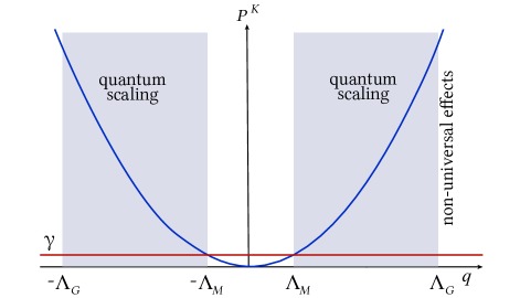
Figure 11: Diffusion noise, $\gamma_{d}q^{2}$ (blue line), and noise gap, $\gamma$ (red line), as a function of momentum. For momentum scales $q\gtrsim\Lambda_{G}$, the renormalization group flow is dominated by nonuniversal effects, while below $\Lambda_{G}$ it is controlled by the nonequilibrium quantum fixed point. For $q\lesssim\Lambda_{M}$, the noise gap $\gamma$ dominates over the diffusion noise, and the quantum scaling regime is left. Figure adapted from Ref. [402].

What is the extent of the quantum scaling regime in momentum space? Quantum scaling can formally be accessed by setting the noise gap to zero, $\gamma\to 0$, or equivalently by working with momenta above the Markov scale $q\gg\sqrt{\gamma/\gamma_{d}}\equiv\Lambda_{M}$, where diffusion noise dominates. Accordingly, the quantum regime will be established between the two momentum scales, $\Lambda_{M}\lesssim q\lesssim\Lambda_{G}$, where $\Lambda_{G}$ is the Ginzburg scale [642]: for $q\lesssim\Lambda_{G}$ corrections to Gaussian scaling become dominant, and the scaling behavior of the system is governed by the Wilson-Fisher fixed point. This situation is sketched in Fig. 11. It is analogous to the conditions for observability of quantum scaling in equilibrium at finite temperature. There, the relevant range of momenta is $\Lambda_{dB}\lesssim q\lesssim\Lambda_{G}$, with $\Lambda_{dB}\sim T^{1/2}$ the de Broglie momentum scale. Temperature, however, is a fixed energy scale, protected against renormalization by the thermal symmetry. In contrast, in our model, $\gamma$ can acquire sizable corrections under RG, which alters the bare value of the Markov scale estimate, $\Lambda_{M}$. The scales $\Lambda_{M,G}$ are nonuniversal and need to be determined for a given microscopic model. Crucially, even after RG corrections are taken into account, $\Lambda_{M}$ remains one order of magnitude smaller than $\Lambda_{G}$ in the model specified above [401].

As indicated in the previous paragraphs, the quantum scaling regime discussed here pertains to a nonequilibrium Bose condensation transition in 1D. However, the following argument shows that the effective dimension of the system in the quantum scaling regime is, in fact, $D=3$, enabling a Bose condensation and spontaneous symmetry breaking phase transition at the point where the sign of $(\gamma_{l}-\gamma_{p})/(\gamma_{l}+\gamma_{p})$ changes even though the spatial dimension of the system is $d=1$. For illustration, we consider the correction to the dissipative spectral gap, $\Delta r_{d}$, but the result would remain unaltered if we were to focus on other couplings. At one-loop order, the correction is given by the tadpole diagram [402]

$$\Delta r_{d}\propto(u_{c}+iu_{d})\int d\omega\,dq\leavevmode\nobreak\ \frac{P^{K}(\omega,q)}{P^{R}(\omega,q)P^{A}(\omega,q)},$$ (97)

where $u_{c}$ and $u_{d}$ are the strength of interactions and two-body loss, respectively (cf. Sec. II.1). In the quantum scaling regime, $P^{K}$ scales quadratically, enlarging the momentum phase space by $q^{2}$ in Eq. (97), and mimicking an integration measure in three dimensions which would also bring an extra quadratic factor ($d^{3}q\sim q^{2}dq$). As a result, the dimensionality of the problem is effectively enlarged by the dynamical critical exponent, $D=d+z=3$. The lack of particle number conservation is crucial: A closed system would have $z=1$, which would still prohibit a condensation transition in $d=1$.

When $\gamma\gg\gamma_{d}q^{2}$, this effective dimensional enlargement does not hold anymore, since $P^{K}$ and $P^{R/A}$ will not scale alike ($P^{K}\sim q^{0}$, $P^{R/A}\sim q^{2}$; classical scaling of Sec. IV.2) and the effective dimensionality of the system will shrink ($D\to d$). In our setup, this corresponds to $D\to 1$, where no continuous symmetry breaking or quantum criticality can occur. Therefore, for momenta $q\lesssim\Lambda_{M}$ (or length scales $l>\Lambda^{-1}_{M}$), the quantum scaling regime is left, as marked in Fig. 11.

XI.2.3 Properties of the nonequilibrium quantum fixed point

At the microscopic scale, our model has the same nonlinear terms as the driven open Bose gas of Eqs. (2) and (3): short-range contact interactions ($u_{c}$) and two-body losses ($u_{d}$). As mentioned above, any quartic combination of fields which respects the $\mathrm{U}_{c}(1)$ symmetry (cf. Sec. IV.1) will be generated in the course of renormalization, irrespective of the number of quantum fields involved. This is different from the semiclassical RG flow of the 3D driven open Bose gas, which retains only the vertex $\left(u_{c}-iu_{d}\right)\psi^{*}_{c}\psi^{*}_{q}\psi^{2}_{c}$ (and its complex conjugate) as RG-relevant nonlinearity. The extra terms include the quantum counterpart of this vertex ($\psi^{*}_{c}\psi^{*}_{q}\psi^{2}_{q}$), multiplicative Markovian noise ($\psi^{*}_{q}\psi_{q}\psi^{*}_{c}\psi_{c}$), and non-Gaussian Markovian noise fluctuations $(\psi^{*}_{q}\psi_{q})^{2}$. As mentioned above, since the system is open ($z=2$) and the upper critical dimension is $d_{c}=2$, the hierarchy of RG-relevant nonlinearities is truncated at fourth order. This is in contrast to isolated, number conserving ($U_{q}$ restored), low-dimensional quantum systems with $z=1$, where all higher-order nonlinearities are equally RG-relevant [225].

The scaling solution of the RG flow in the quantum critical regime is governed by a Wilson-Fisher fixed point with two repulsive directions, associated with simultaneously tuning the spectral gap and the noise gap to zero [402]. This is analogous to thermal equilibrium, where both spectral gap and temperature have to be tuned to zero in order to reach a quantum critical point. The nonequilibrium quantum fixed point is characterized by three key properties:

(1) Asymptotically broken thermal symmetry: The fluctuation-dissipation relation is not restored at infrared scales, since quartic nonlinearities breaking the thermal symmetry of Sec. III.2 have nonzero fixed-point values. This is in contrast to several instances of driven open criticality, where an emergent effective temperature rules the occupation of soft modes [423, 575, 391], cf. also Sec. IV.2 and VIII. We have already encountered in this review instances of criticality where the effective temperature is momentum-dependent at infrared scales and therefore the system spoils fluctuation-dissipation relations (Sec. VIII.2 and [400]). However, in these cases the fixed point is classical (associated to a classical scaling solution).

(2) Absence of decoherence and RG limit cycle: Coherent (spectral gap, interactions, etc.) and dissipative couplings (noise gap, two-body losses, etc.) scale with the same anomalous dimension in the infrared, with their ratios approaching a constant. This signals the absence of decoherence at the Wilson-Fisher fixed point in sharp contrast to the dissipative nature of the semiclassical fixed point, where coherent couplings vanish in the infrared, determining universal decoherence (cf. Sec. VIII and Fig. 12). This is a signature of the dark states supported by the jump operator, which are decoupled from noise in the infrared. The simultaneous presence of coherent and dissipative couplings at the fixed point is further mirrored by slowly damped oscillations in the RG flow of the wave function renormalization $Z$. Similar limit cycle phenomenology is found in coupled Langevin-Ising models (Sec. VIII.2), and in cavity QED with engineered dissipation [530, 529]).

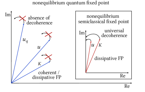
Figure 12: Comparison between the nonequilibrum quantum and classical fixed points (cf. Fig. 6). In the former case ($d=1$), the coherent and dissipative couplings flow under RG to a finite value, which indicates that the system has not fully decohered at the critical point. This is in contrast to the semiclassical fixed point in $d=3$, which displays decoherence at long-wavelengths, with only the dissipative couplings nonvanishing at the fixed point. Figure adapted from Ref. [402].

(3) Absence of quantum-to-classical correspondence: The quantum fixed point is not only without equilibrium analog, but it also does not belong to the same universality class as its 3D driven open counterpart, as follows from the discussion above. This violation of the quantum-to-classical correspondence between low-dimensional ($d=1$) and high-dimensional ($d=3$) criticality is rationalized by noting that the set of RG relevant operators at the Wilson-Fisher fixed point is markedly different in the two cases. Another way to appreciate such sharp discrepancy with a cornerstone of equilibrium criticality [508] is to notice that the equilibrium symmetry is not restored in the quantum case, in contrast to asymptotic thermalization of the semiclassical fixed point. This mismatch in the symmetry properties leads to different universality classes.

XI.2.4 Comparison with noise-driven Luttinger Liquids

The one dimensional driven-open Bose gas has similarities and important differences to the noise-driven Luttinger Liquid discussed in Sec. XI.1. The key difference is that by engineering Markovian noise which scales quadratically with momentum, one can target the quantum scaling limit. The $1/f$ noise used for the Luttinger Liquid is not tailored to access a novel fixed point, and in fact the exponents are non universal in this latter case.

In the model of the driven open Bose gas, particle number conservation is broken by the presence of incoherent gain and loss of particles (the $U_{q}$ symmetry of Sec. IV.1 is broken). These processes do not occur in the Luttinger Liquid of Eq. (92), which evolves under a time-dependent, number-conserving Hamiltonian. The different symmetry properties of the two models result in different soft-mode dispersion relations at criticality (linear for the Luttinger liquid, and quadratic for the open Bose gas), and assign the two systems to different universality classes.

However, what the systems have in common is that the scaling regime of the driven open Bose gas is also cut asymptotically by an emergent effective thermal length ($\Lambda_{M}$), which is generated by the interplay of nonlinearities and dissipation.

XII Universality in dissipative quantum impurities

This section is devoted to the interplay of local dissipative sources and long-wavelength modes in low-dimensional quantum systems. The problem of a quantum impurity, a situation where a few degrees of freedom are locally coupled to an extended interacting quantum systems, is central to the field of strongly correlated systems in equilibrium [225, 392]. It has been key to access prototypical instances of strong-coupling phenomena, which would have been hard to solve in generic conditions, and has provided guidance for decades in solid state and AMO experiments [498].

In a nutshell, distinguishing a few degrees of freedom (the impurity) from the remainder of the system allows us to find nonperturbative phenomena where strong correlations play a role, on the midway between a few-body problem and the full many-particle one. The many-body ‘environment’ serves as a feed of correlations, to which the impurity degrees of freedom couple, leading to a strong intertwining of the two.

In the realm of strongly correlated systems in equilibrium, examples range from the disruptive effects of a local potential embedded in a Fermi sea (Anderson catastrophe [392]), to the strong coupling of magnetic impurities to fermionic or bosonic baths (Kondo effects [491]), and encompass the dressing of static or moving particles in Fermi or Bose-Einstein condensed environments (polarons [258]). This raises the question about the nonequilibrium counterparts of these iconic cases of strongly correlated physics. Studying dissipative quantum impurities elucidates the interplay of dissipation, interactions, and correlations, which is at core of this review. Such impurities can be, for example, local losses, incoherent pumping, or phase noise, embedded in an extended interacting quantum many-body system.

We first consider solvable instances of dissipative impurities (Sec. XII.1). Then, we present a Keldysh approach to treat strongly correlated regimes of interacting wires with local losses (Sec. XII.2).

XII.1 Solvable models of dissipative impurities and the quantum Zeno effect

A phenomenon that is central to the following sections is the quantum Zeno effect [335, 190]. We will start by reviewing its manifestation in solvable systems of dissipative impurities.

Let us consider a tight-binding model of fermions hopping along a one-dimensional chain with one-body loss at the center of the chain, for reference at the lattice site $l=0$ (for analogous setups in spin chains, see Refs. [643, 57, 486, 485, 487, 583, 484, 564]). The corresponding Hamiltonian and jump operator for the dissipative impurity site read

$$\hat{H}=J\sum^{L}_{l=-L}\left(\hat{\psi}^{\dagger}_{l}\hat{\psi}_{l+1}+\text{H.c.}\right),\qquad\hat{L}_{0}=\sqrt{\gamma}\hat{\psi}_{0}.$$ (98)

In the dynamics starting from the ground state of the closed tight-binding model, i.e., a filled Fermi sea, the effect of switching on the loss propagates along the chain, reaching distances $d$ from the impurity on timescales $d/J$ [207]. On smaller distances, a nonequilibrium steady-state is formed. The rate at which fermions leave the system at the impurity site is $r(\gamma)$. It scales as $r(\gamma)\propto\gamma$ for small loss rate ($\gamma\ll J$), while, for strong dissipation $\gamma\gg J$, the rate falls off to zero as $r(\gamma)\sim\gamma^{-1}$ [339, 340, 564]. Due to particle-hole symmetry of the Hamiltonian, analogous results apply when local loss is replaced by gain.

In order to rationalize the counterintuitive decay of $r(\gamma)$ for $\gamma\gg J$, we employ a perturbative argument. The large energy scale set by the loss rate splits the Hilbert space into fast and slow sectors [420, 295]. All states with a particle on the lossy site decay fast with a rate $\sim\gamma$. On the other hand, states with zero occupancy on the dissipative site form the slow sector of the Hilbert space. In second order perturbation theory in the hopping $J$ that couples the slow and fast subspaces, one finds the effective decay rate of states in the slow sector to be $r\sim J^{2}/\gamma$. Another way to rephrase this result is to notice that for $\gamma\gtrsim J$, the speed of particles replenishing the lossy site is smaller than the rate at which they are lost into the environment, leading to a smaller net current flowing toward the dissipative impurity. The dynamical decoupling induced by dissipation finds numerous applications in the engineering of quantum simulators based on ultracold gases, and it is known as quantum Zeno effect [200, 270, 277, 212, 639]. Fig. 13 shows a qualitative dependence of $r(\gamma)$. The RG flow shown in the figure will be discussed in the next section.

To grasp the generality of the phenomenon, one could also consider a chain of spins or fermions subject to a local incoherent scatterer: for instance, the Hamiltonian in Eq. (98) supplemented by a local time-dependent potential $V=\xi(t)\hat{\psi}_{0}^{\dagger}\hat{\psi}_{0}$ with $\xi(t)$ Gaussian white noise [172, 572]. The presence of a fast scale (i.e., dissipation rate), no matter if it is related to loss/pumping or dephasing, will induce the same nonmonotonous behavior. In Ref. [172], the system is initialized in the ground state of Eq. (98) at fixed filling and then the noise is switched on. After the local nonequilibrium state is formed around the impurity, one can observe that the fraction of fermions left inside the Fermi sea grows and then collapses to zero upon increasing the noise strength. This is analogous to the dependence on $\gamma$ discussed above for the case of local losses. The quantum Zeno effect can also manifest in the spreading of correlations or in entanglement dynamics, as reported in studies involving integrable 1D systems [126, 7, 6, 100, 146].

Experimentally, the quantum Zeno effect at dissipative impurities has been demonstrated in a wire of ultracold bosons with an electron beam focused on a small region of space to induce localized loss. In this setup, nonmonotonous behavior of the particle current toward the region of localized dissipation has been observed [79, 49, 348]. There are a number of theory works modelling this scenario. They mostly resort to a semiclassical description of dynamics or Bogoliubov theory, which are appropriate in the presence of a condensate [614, 532, 600]. However, in a wire of interacting fermions, strong correlations could play a decisive role by intertwining with the effect of local dissipation, leading to nontrivial renormalization effects. We will discuss this case in detail in the next section.

Fermionic dissipative impurities can be realized in ultracold atomic wires by mimicking the two-leads scenario typical of mesoscopic physics (experiments [77, 141, 361, 289]; theory [589, 588]). A tightly focused beam at the center of the chain leads to spin-dependent particle losses, with the reservoirs of different spin species used to probe transport across the impurity by imposing a chemical potential difference.

XII.2 Local dissipation in interacting quantum wires:
the dissipative Kane-Fisher problem

Our presentation of the interplay of local dissipation with the quantum fluctuations of a 1D interacting fermionic system will be based on a close analogy with the Kane-Fisher phenomenon. In the latter, a local coherent scatterer acts as a relevant or irrelevant perturbation depending on the repulsive or attractive character of the interactions in the wire prepared in the ground state [225, 478, 312, 314, 313]. Under renormalization, the strength of the impurity grows for repulsive interactions, and the effective long-wavelength description corresponds to a wire split into two decoupled segments. Instead, for attractive interactions, the strength of the impurity diminishes, and the system ‘heals’ itself from the defect. Hence, the conductivity vanishes in the former case and becomes perfect in the latter.

XII.2.1 Qualitative overview: Canonical power counting

The starting, yet crucial, observation is that, after bosonization (cf. also Sec. XII.2.2), the scaling dimensions of a coherent and a dissipative impurity in an interacting fermionic wire are the same. One would then expect, at least on the level of canonical power counting, the same physical picture of the Kane-Fisher problem. Indeed, the RG flow of the rescaled one-body loss rate, $\bar{\gamma}=\gamma/\Lambda$, reads [206]

$$\frac{d\bar{\gamma}}{d\ell}=\left(1-g\right)\bar{\gamma},$$ (99)

where $g$ is the Luttinger parameter of the wire. From this flow equation we retrieve the physical picture discussed above. For attractive interactions in the wire ($g>1$) dissipation is renormalized to zero and the impurity becomes transparent; in contrast, for repulsive interactions ($g<1$), the dissipation strength flows to infinity, invalidating perturbative RG. However, in this case, we can approach the problem from a complementary angle, which leads to an RG equation valid for the inverse of $\gamma$ [206]. Its rescaled value is defined as $\bar{D}=\Lambda/\gamma$ and obeys the RG flow

$$\frac{d\bar{D}}{d\ell}=\left(1-g^{-1}\right)\bar{D}.$$ (100)

In this second case, one assumes a strong dissipative impurity, treating the remainder of the chain as a perturbation. This is analogous to a similar approach in the RG treatment of the original Kane-Fisher problem [16, 315], and to the perturbative argument outlined for the Zeno effect in Sec. XII.1. The RG flow in Eq. (100) implies that for repulsive interactions ($g<1$), the weak link is cut $\bar{D}\to 0$, while for attractive interactions, $\bar{D}$ is renormalized to infinity, invalidating the RG treatment. This discussion is summarized in Fig. 13. In the following, we will refer to the two fixed points $\gamma\to\infty$ and $\gamma\to 0$ as fluctuation-induced quantum Zeno (FIQZ) effect and fluctuation-induced transparency (FIT), respectively. This nomenclature is due to the fact that no fine-tuning of driving parameters is required to reach these two fixed point; it rather roots in the presence of gapless modes in the wire. These new universal regimes are purely fluctuation driven: it is the nature of interactions in the chain ($g$ smaller or larger than one), which determines the onset or lack of the Zeno effect.

Figure 13: Dependence of the escape rate $r$ on the microscopic loss rate at the impurity site $\gamma$. When $\gamma$ is large, $r$ drops to zero, which is a manifestation of the quantum Zeno effect. The red and blue arrows qualitatively portray the RG flow of an interacting fermionic wire with localized loss, leading to the two fixed points achieved for repulsive and attractive interactions, respectively. Figure adapted from Ref. [206].

XII.2.2 Keldysh field theory of the dissipative Kane-Fisher problem

We now turn our attention to the interplay of fluctuations and localized dissipation, going beyond canonical power counting. The key new ingredient here is that, similar to the equilibrium impurity problems, the interplay between interactions and a continuum of gapless modes strongly renormalizes the couplings. The couplings still flow to either of the two fixed points of Fig. 13 (FIT or FIQZ). However, now the system may also enter a thermalizing phase where it heats up and no fluctuation-induced phenomena can establish. This is the physical picture encapsulated in Fig. 14, which we substantiate in the following.

This case of study is, indeed, a clear example of emergent nonequilibrium physics in the quantum regime resulting from the interplay of long-wavelength modes, dissipation, and strong many-body interactions, which can be addressed with the nonequilibrium RG approach widely employed in this review. We consider the continuum Luttinger liquid description of a fermionic wire [207]

$$\hat{H}=\frac{v}{2\pi}\int_{x}\left[g\left(\partial_{x}\hat{\phi}\right)^{2}+g^{-1}\left(\partial_{x}\hat{\theta}\right)^{2}\right],$$ (101)

with $\hat{\theta}$ and $\hat{\phi}$ describing density and phase fluctuations, and $v$ the velocity of sound. At the center of the wire at $x=0$, there is a single-body fermion loss modeled by the Lindblad jump operator, $\hat{L}(x=0)=\sqrt{\gamma}\hat{\psi}(x=0)$, which in bosonization language is given by

$$\hat{\psi}(x=0)\approx e^{i(\hat{\phi}+\hat{\theta})|_{x=0}}+e^{i(\hat{\phi}-\hat{\theta})|_{x=0}}.$$ (102)

Here we have retained only leading harmonics. Analogously to the treatment of the usual Kane-Fisher problem [313], one can integrate out the chain at all points $x\neq 0$ to obtain an effective action for the impurity, reducing the extended system to a $0+1$-dimensional problem. This is feasible analytically due to the quadratic nature of the Luttinger liquid Hamiltonian (101). Physically, the remainder of the chain acts as a bath for the impurity degrees of freedom, which can then be treated in an RG approach. We thus obtain a contribution to the Keldysh action at $x=0$ in the form of an effective Caldeira-Leggett bath [105] which describes the effect of the remainder of the chain on the impurity as an environment:

$${S^{B}}|_{x=0}=\frac{i}{\pi}\int_{\omega}\left(\theta^{*}_{c}\leavevmode\nobreak\ \theta^{*}_{q}\right)\begin{pmatrix}0&-\kappa\omega\\ \kappa\omega&2\kappa_{0}|\omega|+4\kappa T_{\text{eff}}\end{pmatrix}\begin{pmatrix}\theta_{c}\\ \theta_{q}\end{pmatrix}.$$ (103)

In the expression above, the damping term in the retarded and advanced sectors is proportional to $\kappa=1/g$, while $T_{\text{eff}}$ accounts for the possibility of generating an effectively temperature under RG transformations (cf. Sec. XI.1), which is the noise gap in the language of Sec. IV.2. While the damping coefficient $\kappa$ in the retarded and advanced sectors can grow under renormalization, the corresponding term in the Keldysh sector will remain at its microscopic value ($\kappa_{0}$) since perturbative corrections cannot generate a nonanalytic function of the frequency ($\propto|\omega|$).

The master equation with jump operator Eq. (102) adds to the free Keldysh action in Eq. (103) the nonlinear term

$$S^{I}|_{x=0}=-2i\gamma\int_{t,x}\delta(x)\left[\left(e^{i\sqrt{2}\phi_{q}}-\cos\!\left(\sqrt{2}\theta_{q}\right)\cos\!\left(\sqrt{2}\theta_{c}\right)\right)\right.\\ \left.+\left(e^{i\sqrt{2}\phi_{q}}\cos\!\left(\sqrt{2}\theta_{q}\right)-1\right)\right].$$ (104)

Therefore, the total Keldysh action of the problem at the impurity site $S|_{x=0}$ consists of the sum of the nonlinear term coming from local dissipation, and of the environment action, $S|_{x=0}=S^{I}|_{x=0}+S^{B}|_{x=0}$.

Figure 14: Phase diagram for a dissipative impurity in an interacting fermion wire from second order RG equations, for different values of the microscopic dissipation strength $\bar{\gamma}_{0}$ ($\bar{D}_{0}$ in the dual regime) and of the Luttinger parameter $g$. The blue-shaded area in the lower-right corner corresponds to values where the fluctuation-induced transparency (FIT) is visible, while the upper-left one corresponds to values where the fluctuation-induced quantum Zeno effect (FIQZ) is visible. The gray-shaded areas correspond to values where the effective temperature suppresses these effects. The white regions correspond to values where the perturbative RG breaks down. Figure adapted from Ref. [207].

Performing an RG analysis up to second order in $\gamma$ on the total action $S|_{x=0}$, one finds a non-trivial RG flow of $\gamma$, $\kappa$ and $T_{\mathrm{eff}}$ (the RG flow is initialized at zero effective temperature; an analogous procedure can be carried out for the dual theory at large $\gamma$). The first order calculation reproduces the discussion above in Sec. XII.2.1. At second order, fluctuations lead to a flow of $\kappa$ and, importantly, to the emergence of a finite effective temperature $T_{\mathrm{eff}}$, corrupting the zero temperature scaling solution (recall that the system is out of equilibrium, therefore the thermal symmetry does not protect temperature from renormalization, cf. Secs. III.2, VIII, XI). This allows one to study quantitatively how the interplay of local heating and nonlinearity destroy the two fluctuation-induced regimes, the FIT and FIQZ. This analysis [207] is analogous to the comparison of the Ginzburg and de Broglie scales in the context of quantum criticality, discussed in detail in Sec. XI. Namely, for certain microscopic values of $g$ and $\gamma$ (gray regions in Fig. 14), the length scale at which thermal fluctuations are dominant is smaller than the typical length where one can observe the renormalization of the dissipation strength; this implies that the FIT and FIQZ are not observable in those parameter windows. (In addition, there are the regions of instability of RG which match the result at the level of canonical power counting, white in Fig. 14.) A simple physical picture emerges: Interactions have to be strong ($|g|$ large) to make these two effects visible in experiment [207, 434]. In these regions, the picture of Fig. 13 remains qualitatively correct, yet quantitatively altered by higher-order fluctuations.

A real-space RG calculation of transmission and reflection coefficients, similarly to the traditional Kane-Fisher problem [411, 625], leads to conclusions consistent with the momentum-space RG discussed above. The real-space RG, working directly with fermionic degrees of freedom, has the advantage of being more suitable for comparison with numerical approaches to the problem [207, 617].

XIII Universality in fermion systems

In the previous section, we have made a first encounter with fermions in the context of impurity problems, where the nonequilibrium perturbation was restricted to a single point in space. Here, we continue our discussion of fermions, but we return to setups of driven open quantum matter as discussed in earlier sections, where out of equilibrium dynamics occurs everywhere in space. Quantum mechanics must be expected to play a crucial role, as by the fermionic exclusion principle there is no simple classical limit. We review elements of universality in driven open fermion systems, and connect them to the basic principles that underlie this review: pure vs. mixed states, the impact of equilibrium vs. nonequilibrium generators of dynamics, and the presence of strong symmetries.

A key additional ingredient, encountered only tangentially in the form of vortex defects in Secs. VII.3 and VII.4.3 so far, is topology. In particular, we will highlight that topology enables universality, in that it leads to macroscopic behavior that is highly insensitive to the microscopic generator of dynamics, and robust with respect to the state of the system being pure or mixed in a sense made precise below.

To this end, we first discuss a scenario to create out-of-equilibrium analogs of fermionic ground- and finite temperature states, which are equipped with a nontrivial topology (Sec. XIII.1), and thus give rise to nonequilibrium analogs of topological insulators and superconductors [276, 493, 130]. This is achieved by a suitable design of the jump operators. Pure stationary states can be generated as dark states of Lindblad dynamics. When different sets of Lindblad operators are put into competition, topological phase transitions ensue, which can proceed in pure or mixed states. Although a comprehensive picture of such phase transitions—and more generally, nonequilibrium phase transitions of fermions—is still outstanding, one particular aspect becomes clear already: Critical fermions can exist only in pure states, analogous to thermodynamic equilibrium [508]. We then continue to overview in Sec. XIII.2 that topology (1) ‘beats dynamics’, i.e., it is insensitive to whether generators of dynamics describe in- or out-of-equilibrium situations, and that it also (2) ‘beats mixedness’, i.e., topological quantization persists in suitable mixed state observables. In both cases, a universal topological gauge theory emerges, which describes physically observable quantized (albeit generally nonlinear) responses, and entails a bulk-boundary correspondence. We close with a discussion of fundamental discrete symmetry operations such as time reversal and particle-hole transformations, pointing out a dynamical fine structure in their implementation, depending exclusively on whether the generator of dynamics obeys the thermal symmetry of Sec. III.2 or not (Sec. XIII.3).

XIII.1 Topological phase transitions of fermions out of equilibrium: pure vs. mixed states

The nonequilibrium analog of ground states of Hamiltonians are dark states of Lindbladians: Both scenarios feature pure states, but are prepared by dynamics respecting or violating equilibrium conditions, respectively, as per the discussion in Sec. III. We have encountered instances of dark states already in Secs. X and XI.2 (see also Appendix D for a more detailed discussion). These states, represented by a pure density matrix $\hat{\rho}_{D}=\lvert D\rangle\langle D\rvert$, are annihilated by the Lindbladian in Eq. (1), $\mathcal{L}\hat{\rho}_{D}=0$, via satisfying the two conditions

$$\hat{H}\lvert D\rangle=E\lvert D\rangle\quad\text{and}\quad\hat{L}_{l}\lvert D\rangle=0\quad\forall l.$$ (105)

Here, $l$ is a multi-index, which will be made concrete below; we will consider the case $\hat{H}=0$ for simplicity. Once such a state is reached, time evolution stops and the system becomes stationary; when the dark state is unique and no other stationary solutions exist, the dark state will be reached from an arbitrary initial (and possibly mixed) state (cf. Appendix D). This circumstance can be used for state preparation in quantum optics [479] and many-body physics [166, 585], including for topological states [167]. Below we will consider a class of Lindbladians featuring a dark state with such topological properties. Topological phase transitions result from the competition between Lindbladians that stabilize topologically distinct dark states. These transitions are nonequilibrium analogs of quantum and classical topological phase transitions, proceeding in pure and mixed states, respectively.

XIII.1.1 Lindbladians with a topological dark state

For concreteness, we focus here on dark states representing two-banded topological insulators in one dimension in a translationly invariant setting; such models have been introduced in Refs. [239, 539]. This scenario can be generalized to arbitrary dimension [290]. It also comprises topological superfluids [169, 622, 167, 47, 46, 287], see [46] for a review. Such topological dark states are stabilized by a Lindbladian Eq. (1) with Lindblad operators of the form

$$\hat{L}_{a,1,i}=\hat{\psi}^{\dagger}_{a,i}\hat{l}_{1,i},\quad\hat{L}_{a,2,i}=\hat{\psi}_{a,i}\hat{l}^{\dagger}_{2,i},\quad\hat{l}_{a,i}=\sum_{b,j}U_{ab,ij}\hat{\psi}_{b,j}.$$ (106)

Here, $a,b\in\{1,2\}$ label the band index, and $i,j$ are lattice site indices. The operators $\hat{l}_{a,i}$ are superpositions of the local annihilation operators $\hat{\psi}_{a,i}$. They are related to the latter by the unitary, canonical transformation $U$, which encodes the topological properties, see below. When the transformation $U$ is not exactly local, the dark state carries real-space entanglement, unlike the state considered in Sec. V.1. The operators in Eq. (106) uniquely [341] stabilize the Gaussian, half filled dark state

$$\lvert D\rangle=\prod_{i}\hat{l}_{2,i}^{\dagger}\lvert 0\rangle,\quad\hat{L}_{a,1,i}\lvert D\rangle=\hat{L}_{a,2,i}\lvert D\rangle=0\quad\forall\quad a,i.$$ (107)

The annihilation of the dark state by the Lindblad operators happens due to distinct mechanisms (see Fig. 15(a)): $\hat{L}_{a,1}$ annihilates the dark state since there are no particles in superposition $\hat{l}^{\dagger}_{1,i}$, and $\hat{L}_{a,2,i}$ due to Pauli blocking for particles in superposition $\hat{l}^{\dagger}_{2,i}$. Once the state is annihilated by the $\hat{l}_{1,i}$ and $\hat{l}^{\dagger}_{2,i}$ pieces in the Lindblad operators, the evolution stops. If the state is not annihilated, it is recycled into the evolution until it is annihilated, by the uniqueness of the dark state and the absence of other stationary solutions in the present problem.

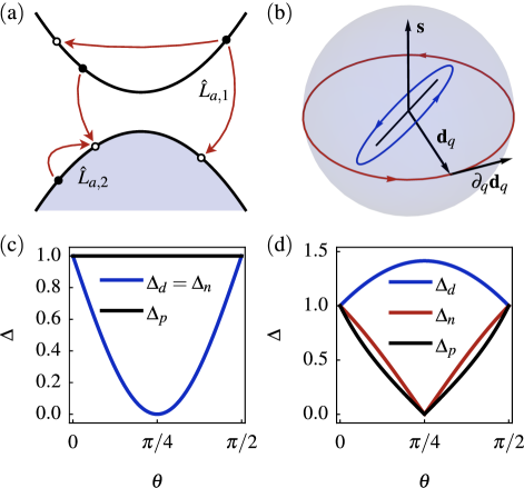
Figure 15: (a) Action of Lindblad operators: $\hat{L}_{a,1}$ annihilate particles in the upper band to either recreate them in the lower band or redistribute them in the upper band. Similarly, $\hat{L}_{a,2}$ create particles in the lower band by transfer from the upper or redistribution in the lower band (adapted from Ref. [571]). (b) Winding number and purity gap closing: Pure states are characterized by $|\mathbf{d}_{q}|=1\Leftrightarrow\Gamma_{q}^{2}=\mathbbm{1}$ for all $q$. Then, $\mathbf{d}_{q}$ lies on a grand circle of the Bloch sphere in the presence of a chiral symmetry ($\mathbf{s}\perp\mathbf{d}_{q}\Leftrightarrow\{\Sigma,\Gamma_{q}\}=0$ for all $q$, red line). For mixed states, $|\mathbf{d}_{q}|<1$ (blue line). The closing of a purity gap then corresponds to a zero in $|\mathbf{d}_{q}|$ for at least one $q$ (black straight line). At such a point, the geometry of an ellipse, for which a winding number is well defined, collapses to a line. No winding can then be defined, which signals a topological phase transition. (c),(d) Dissipative ($\Delta_{d}$), noise ($\Delta_{n}$), and purity gaps ($\Delta_{p}$) for topological quantum (c) and classical (d) phase transitions. $\Delta_{d}$ and $\Delta_{n}$ are measured in units of $\bar{\gamma}$, $\Delta_{p}$ is dimensionless. Discussion, see text.

The jump operators Eq. (106) conserve the total particle number, $[\hat{L}_{a,1/2,i},\hat{N}]=0$, as it should be for operators that stabilize an insulating state (there is a strong $\mathrm{U}_{q}(1)$ symmetry in the associated field theory). Insisting on this property makes the Lindbladian necessarily quartic in the field operators, and thus interacting. An alternative version with Lindblad operators $\hat{L}_{a,1,i}=\hat{l}_{1,i}$ and $\hat{L}_{a,2,i}=\hat{l}^{\dagger}_{2,i}$ stabilizes the same dark state, but does not conserve particle number, although it still exhibits a weak $\mathrm{U}_{c}(1)$ symmetry.

The number nonconserving operators can also be viewed as a mean-field approximation to the full interacting Lindblad dynamics, valid at late times when the dynamics can be linearized around the exactly known dark state. Mean-field theory can be implemented within the operator formalism [46] or in the functional integral representation [571]. The latter lends itself to extracting beyond mean-field physics, see Sec. XIII.2 below. In a functional integral representation, mean-field theory has the status of a one-loop self-consistent Born approximation [16]. It results in a simple replacement of the overall decay rate $\gamma\to\bar{\gamma}=2n\gamma$, where $n=1/2$ for half filling as in Eq. (107). The effective mean-field Gaussian action with $l=(l_{1},l_{2})^{{\mathchoice{\raisebox{0.0pt}{$\displaystyle\intercal$}}{\raisebox{0.0pt}{$\textstyle\intercal$}}{\raisebox{0.0pt}{$\scriptstyle\intercal$}}{\raisebox{0.0pt}{$\scriptscriptstyle\intercal$}}}}$ and in the frequency-momentum domain then reads

$$\begin{gathered}S=\int_{\omega,q}\left(l_{c}^{*{\mathchoice{\raisebox{0.0pt}{$\displaystyle\intercal$}}{\raisebox{0.0pt}{$\textstyle\intercal$}}{\raisebox{0.0pt}{$\scriptstyle\intercal$}}{\raisebox{0.0pt}{$\scriptscriptstyle\intercal$}}}},l_{q}^{*{\mathchoice{\raisebox{0.0pt}{$\displaystyle\intercal$}}{\raisebox{0.0pt}{$\textstyle\intercal$}}{\raisebox{0.0pt}{$\scriptstyle\intercal$}}{\raisebox{0.0pt}{$\scriptscriptstyle\intercal$}}}}\right)\left(\begin{array}[]{cc}0&P^{A}(\omega,q)\\ P^{R}(\omega,q)&P^{K}(q)\end{array}\right)\left(\begin{array}[]{c}l_{c}\\ l_{q}\end{array}\right),\\ P^{R}(\omega,q)=\left(\omega+i\bar{\gamma}_{q}\right)\mathbbm{1},\quad P^{K}({q})=2i\bar{\gamma}_{q}\sigma_{z},\end{gathered}$$ (108)

with damping rate $\bar{\gamma}_{q}\geq 0$. Due to the weak $\mathrm{U}_{c}(1)$ symmetry of the number nonconserving mean-field theory, the action does not contain pairing terms such as $l_{1,c}l_{1,q}$, which are included in the general Nambu structure of Gaussian actions discussed in Appendix C. The action Eq. (108) will allow us to discuss the basic properties of nonequilibrium topological phase transitions. The noise matrix $P^{K}$ is not positive definite—unlike for bosons, $P^{K}>0$ is not required for convergence of the fermionic functional integral. The positive eigenvalue of $P^{K}$ indicates that the modes $l_{1}$ are empty; the negative eigenvalue indicates that the modes $l_{2}$ are occupied. This results from the different ordering of $l_{1,q}^{*}l_{1,q}$ vs. $l_{2,q}l_{2,q}^{*}=-l_{2,q}^{*}l_{2,q}$. Using $l(\omega,q)=U_{q}\psi(\omega,q)$ with $\psi=(\psi_{1},\psi_{2})^{{\mathchoice{\raisebox{0.0pt}{$\displaystyle\intercal$}}{\raisebox{0.0pt}{$\textstyle\intercal$}}{\raisebox{0.0pt}{$\scriptstyle\intercal$}}{\raisebox{0.0pt}{$\scriptscriptstyle\intercal$}}}}$ in the Fourier representation (cf. Eq. 106), the action can be expressed in terms of the original lattice fermion fields. In this basis, $P^{R/A}(\omega,q)$ continue to be unit matrices, but $P^{K}(q)\to 2i\bar{\gamma}U_{q}^{\dagger}\sigma_{z}U_{q}$ becomes a general anti-Hermitian matrix, with the structure of a free topological Hamiltonian up to the imaginary prefactor. The topology is thus encoded in the noise matrix in dissipatively stabilized topological states of fermions.

The above discussion applies in a translationally invariant setting and discards edge mode effects, which lead to topological degeneracy and higher dimensional dark spaces. We refer to Refs. [46, 14, 513, 220, 221] for a discussion of these aspects.

XIII.1.2 Phase transitions

Topological phase transitions are defined by an abrupt jump of an integer-valued topological invariant as a function of parameter changes. We consider here a simple model with a stationary state of Su-Schrieffer-Heeger type [560], equipped with a chiral symmetry, and topologically characterized by a chiral winding number invariant. The invariant can be constructed based on the covariance matrix collecting the single-particle correlation functions $\Gamma_{{q}}=i\int\frac{d\omega}{2\pi}G^{K}(\omega,{q})$, where $G^{K}=-G^{R}P^{K}G^{A}$ can be read off Eq. (108). The winding number is then defined as

$$W=\int_{-\pi}^{\pi}\frac{dq}{2\pi}\mathop{\mathrm{tr}}\!\left(\Sigma\Gamma^{-1}_{q}i\partial_{q}\Gamma_{q}\right),$$ (109)

where the chiral symmetry is expressed by the constraint that there exist a Hermitian matrix $\Sigma$ such that $\{\Sigma,\Gamma_{q}\}=0$ for all $q$. The winding is illustrated in Fig. 15(b), where we represent the matrices in terms of vectors according to $\Gamma_{q}=\mathbf{d}_{q}\cdot\boldsymbol{\sigma},\Sigma=\mathbf{s}\cdot\boldsymbol{\sigma}$ ($\boldsymbol{\sigma}$ collects the Pauli matrices). A winding number of $W=+1$ corresponds to $\mathbf{d}_{q}$ encircling $\mathbf{s}$ once in counterclockwise direction upon $q=-\pi\to\pi$. For example, a model defined with quasi-local operators

$$\begin{pmatrix}\hat{l}_{1,i}\\ \hat{l}_{2,i}\end{pmatrix}=\frac{1}{\sqrt{2}}\begin{pmatrix}\hat{\psi}_{1,i+1}+\hat{\psi}_{2,i}\\ -\hat{\psi}_{1,i+1}+\hat{\psi}_{2,i}\\ \end{pmatrix},$$ (110)

has the covariance matrix $\Gamma_{q}=e^{-iq}\sigma^{+}+e^{iq}\sigma^{-}$, $\Sigma=\sigma^{z}$, and the winding $W=+1$. The opposite winding $W=-1$ results from operators $\hat{r}_{1,i}$ and $\hat{r}_{2,i}$, obtained upon exchanging $\hat{\psi}_{1,i+1}\to\hat{\psi}_{1,i}$ and $\hat{\psi}_{2,i}\to\hat{\psi}_{2,i+1}$ in the above equation.

Topological phase transitions with a jump $W=+1\to-1$ can be generated by putting the operators $\hat{l}$ and $\hat{r}$ into competition. To understand the basic properties of these transitions, it is sufficient to study the linearized model, described by the Gaussian action Eq. (108). The abrupt change of the topological invariant can occur in two ways: A first option is a closing of the dissipative gap, which is analogous to the closing of the energy gap in the ground state of Hamiltonian systems. A second one is the closing of the noise and purity gaps. The latter case is illustrated in Fig. 15(b), straight black line inside the Bloch sphere. Indeed there are two qualitatively distinct transitions reflecting these two options, which occur in pure or mixed states, respectively:

(i) Topological quantum phase transition (in a pure dark state). We set the operators $\hat{l}$ and $\hat{r}$ into competition by means of a coherent superposition of operators,

$$\hat{x}_{a,i}=\cos(\theta)\hat{l}_{a,i}+\sin(\theta)\hat{r}_{a,i},$$ (111)

with the limiting cases $\hat{x}=\hat{l}$ for $\theta=0$ and $\hat{x}=\hat{r}$ for $\theta=\pi/2$. For any value of $\theta\in[0,\pi/2]$, the Lindbladian with jump operators $\hat{x}$ has a dark state given by $\lvert D\rangle=\prod_{i}\hat{x}^{\dagger}_{2,i}\lvert 0\rangle$. Upon tuning $\theta=0\to\pi/2$, a topological phase transition is crossed, where the winding number jumps from $W=+1\to-1$. The dissipative gap $\Delta_{d}$ and the noise gap $\Delta_{n}$ (cf. Sec. IV.2), which are determined by $P^{R}(\omega,q)$ and $P^{K}(q)$ given in Eq. (108) directly in the diagonal basis, are shown in Fig. 15(c). At the transition at $\theta=\pi/4$, the gaps close, $\Delta_{d}=\Delta_{n}=0$. The fact that the steady state is a pure dark state for all values of $\theta$ is reflected in the constant value $\Delta_{p}=1$ of the purity gap, which is defined in terms of the eigenvalues $\lambda_{a,q}$ of the covariance matrix,

$$\Delta_{p}=\min_{a,q}\left\lvert\lambda_{a,q}\right\rvert.$$ (112)

This definition implies that a state with a vanishing purity gap features at least one fermionic mode in a totally mixed (infinite temperature) state.

(ii) Topological classical phase transition (in a mixed state). Now we consider a competition by means of an incoherent sum of operators, in terms of a Lindblad generator

$$\mathcal{L}=\cos(\theta)\mathcal{L}_{l}+\sin(\theta)\mathcal{L}_{r},$$ (113)

where $\mathcal{L}_{l}$ features Lindblad operators involving $\hat{l}$, and analogously for $\mathcal{L}_{r}$; again we set $\hat{H}=0$. In this case, the stationary state is known exactly only in the cases $\theta=0,\pi/2$, where the steady state is given by the respective dark states of opposite winding number. In between, the stationary state is mixed. However, the chiral symmetry is preserved [14], and there must be a topological phase transition. This behavior is captured by an effective linear model, with a generator of dynamics which is a weighted direct sum of the $l$ and $r$ models [290]. The dissipative, noise, and purity gaps are shown in Fig. 15(d). The dissipative gap is finite for $0\leq\theta\leq\pi/2$. However, both noise and purity gaps close at $\theta=\pi/4$. At this point, the momentum modes $q=\pm\pi/2$ are in a fully mixed state. The winding number evaluates to $W=+1$ for $0\leq\theta<\pi/4$ and to $W=-1$ for $\pi/4<\theta\leq\pi/2$. In these regions, the purity gap is open. The integrity of a winding number defined in Eq. (109) is verified straightforwardly under this condition. Indeed, intuitively, the number of windings of the vector $\mathbf{d}_{q}$ is well-defined until the circle is deformed to a line or point, which can only happen once the purity gap closes. The collapse of the purity gap is illustrated in Fig. 15(b), as already mentioned above. In summary, the transition happens when the noise and, consequently, the purity gap close, while the dissipative gap remains open. This yields a topological phase transition without thermodynamic signatures, such as divergent length or time scales.

For fermions, the topological (i) quantum and (ii) classical phase transitions are the only types of transitions that can occur: Since the spectrum of $\Gamma$ is bounded between $-1$ and $1$ by the Pauli principle, there cannot be a transition where the dissipative gap closes, while the noise gap remains open. Transitions with divergent length and time scales for the fermion degrees of freedom are possible only in pure states. Topological phase transitions are possible in mixed states, but they proceed without thermodynamic signatures. This is a general consequence of Fermi statistics, applies in and out of equilibrium, and includes interacting systems. The absence of critical fermions in mixed states is seen perhaps more straightforwardly at thermodynamic equilibrium: In a Euclidean functional integral formulation, the fermionic Matsubara frequencies are characterized by odd integers, $\omega_{n}=\left(2n+1\right)\pi/\beta$ with $n\in\mathbb{Z}$ [642], and do not allow for zero modes of the inverse fermion Green’s function at nonzero temperature.

The concept of purity gaps and their closing as enabling topological transitions is not bound to nonequilibrium problems. However, at thermal equilibrium, the circumstances under which a purity gap can close are more restrictive, since all modes experience the same temperature by the principle of detailed balance: The covariance matrix (for a Gaussian problem for definiteness) is $\Gamma=\tanh(\beta H)$, with inverse temperature $\beta$ and (first quantized) Hamiltonian $H$. Zero modes of $\Gamma$, signalling the purity gap closing, can only occur if there are zero modes of $H$ for finite temperature, or for infinite temperature $\beta=0$ in the absence of zero modes of $H$.

We close with a comment on the nature of the pure state phase transitions in the present models. Due to the specific choice of Gaussian dark states, all static correlation functions in stationary state can be computed exactly, including at the critical point. The corresponding static exponents are thus Gaussian. However, since the generator of dynamics is interacting, this does not imply that the dynamic exponent is Gaussian as well (one example where a non-Gaussian dynamic and Gaussian static exponents are realized is provided by the KPZ equation in one dimension, cf. [566, 311]). A general analysis of out-of-equilibrium fermion criticality is outstanding.

XIII.2 Universality of topological response out of equilibrium

In equilibrium ground states, topology is encoded in the ground-state wave function, i.e., in the state of the system. A fundamental question is then, how topological structures generalize once the realm of ground states is left. This may concern (i) the breaking of equilibrium conditions while preserving the pure state nature analogously to a ground state, and (ii) giving up purity, in- and out of equilibrium.

An overarching framework to address this question is topological field theory [635, 381, 338, 492]. Based on the interplay of topology and gauge structures, effective theories provide a bridge between microphysics and observable macrophysics [635, 381, 495, 504]. Where gauge principles exist, they show a high level of robustness, including in the presence of interactions [504] or translational symmetry breaking [13]. Indeed, general adiabatic gauge principles have been identified for nonequilibrium Lindblad dynamics in a series of seminal works [32, 34, 33, 8]. Here, we specialize to the case of $\mathrm{U}(1)$ gauge theory, which also allows one to directly study the physical consequences of the gauge structure in many-body systems.

XIII.2.1 Universality of topological response: equilibrium vs. nonequilibrium dynamics

We consider the nonequilibrium analog of a Chern insulator in two dimensions, described by a wave function $\lvert D\rangle$. As above, this scenario is realized by choosing Lindblad operators such that $\lvert D\rangle$ is their dark state. Then the stationary state $\lvert D\rangle$ is equivalent to the equilibrium ground state of a suitably chosen Hamiltonian, while the dynamics of the system differs from the Hamiltonian evolution. More precisely, we require the following: $\lvert D\rangle$ should

(i) be unique, such that $\hat{\rho}_{D}=\lvert D\rangle\langle D\rvert$ is a pure state;

(ii) be stable, so that local perturbations to the steady state relax at a finite minimal rate, i.e., there is a dissipative (many-body) gap;

(iii) result as the stationary state of a particle number conserving dynamics, implemented by the presence of a strong $\mathrm{U}_{q}(1)$ symmetry.

This implements the conditions required by Laughlin’s gauge argument [358]: the threading of a quantum Hall annulus by a time varying magnetic flux can be adiabatic only if the bulk state is nondegenerate and has a (many-body) spectral gap. Then, the insertion of flux quanta will lead to the transfer of an integer number of charges from one edge to the other, provided these charges cannot be lost (e.g., to a bath).

The above requirements are met by a choice of Lindblad operators of the same structure as considered in the preceding section (working in the spatial continuum here, and with overall damping rate $\gamma$): $\hat{L}_{a,1}=\hat{\psi}_{a}\hat{l}_{1}$ and $\hat{L}_{a,2}=\hat{\psi}_{a}\hat{l}^{\dagger}_{2}$, where in momentum space ($\hat{l}=(\hat{l}_{1},\hat{l}_{2})^{{\mathchoice{\raisebox{0.0pt}{$\displaystyle\intercal$}}{\raisebox{0.0pt}{$\textstyle\intercal$}}{\raisebox{0.0pt}{$\scriptstyle\intercal$}}{\raisebox{0.0pt}{$\scriptscriptstyle\intercal$}}}}$)

$$\hat{l}_{\mathbf{q}}=V_{\mathbf{q}}\hat{\psi}_{\mathbf{q}},\quad V_{\mathbf{q}}=q_{x}\mathbbm{1}+iq_{y}\sigma_{z}+im\sigma_{y}\equiv d^{1/2}_{\mathbf{q}}U_{\mathbf{q}}.$$ (114)

The transformation $V$ is local in real space, $V_{\mathbf{x}}=-i\partial_{x}\mathbbm{1}-\partial_{y}\sigma_{z}+im\sigma_{y}$, such that the Lindblad operators $\hat{L}$ share this property, and $d_{\mathbf{q}}=q^{2}+m^{2}$ with $q=\left\lvert\mathbf{q}\right\rvert$ is a normalization factor introduced here to ensure that $U_{\mathbf{q}}$ is unitary. The dark state targeted by these Lindblad operators coincides with the ground state of the Hamiltonian $\hat{H}=\int_{\mathbf{q}}\hat{\psi}^{\dagger}_{\mathbf{q}}\mathbf{d}_{\mathbf{q}}\cdot\boldsymbol{\sigma}\hat{\psi}_{\mathbf{q}}=\int_{\mathbf{q}}\hat{l}^{\dagger}_{\mathbf{q}}\sigma_{z}\hat{l}_{\mathbf{q}}$, with $\mathbf{d}_{\mathbf{q}}=(2mq_{x},2mq_{y},-m^{2}+q^{2})^{{\mathchoice{\raisebox{0.0pt}{$\displaystyle\intercal$}}{\raisebox{0.0pt}{$\textstyle\intercal$}}{\raisebox{0.0pt}{$\scriptstyle\intercal$}}{\raisebox{0.0pt}{$\scriptscriptstyle\intercal$}}}}$ such that $d_{\mathbf{q}}=\left\lvert\mathbf{d}_{\mathbf{q}}\right\rvert$. Similar to the discussion in Sec. XIII.1, the winding of the map $\mathbf{q}\mapsto\mathbf{d}_{\mathbf{q}}$ defines a Chern number $\theta=-1$ for any $m\neq 0$.

A gauge field is introduced by minimal coupling in the field theory framework: This is enabled by the strong $\mathrm{U}_{q}(1)$ symmetry associated with particle number conservation, which translates to independent transformations $\psi_{\pm}(t,\mathbf{x})\mapsto e^{i\theta_{\pm}}\psi_{\pm}(t,\mathbf{x})$ on each contour. Promoting global to local gauge invariance under transformations $\theta_{\pm}(t,\mathbf{x})$ then requires us to introduce gauge fields appearing in covariant derivatives $\partial_{\mu}\to\partial_{\mu}-iA_{\pm,\mu}$, where $\mu\in\{t,x,y\}$. Up to terms that are topologically trivial, this replaces the Lindblad operators by, e.g.,

$$L_{1,1}\to L_{1,1}+\psi^{\dagger}_{1}\left(a_{i}l\right)_{1}A_{\pm,i}+\dotsb,\quad a_{i}=\left(i\partial_{q_{i}}U_{\mathbf{q}}\right)U_{\mathbf{q}}^{\dagger},$$ (115)

where $a_{i}$ ($i=x,y$) is a Berry connection represented in momentum space on the right, encoding the topology of the problem. Indeed, in a mean-field theory for the fermions as described above, followed by a gradient expansion of the fermionic Gaussian functional integral to lowest order, a Chern-Simons theory on the Keldysh contour emerges,

$$S[A_{\pm}] =\frac{\theta}{4\pi}\int_{t,\mathbf{x}}\left[\epsilon^{\mu\nu\rho}\left(A_{+,\mu+}\partial_{\nu}A_{+,\rho}-A_{-,\mu}\partial_{\nu}A_{-,\rho}\right)+\dotsb\right],$$

$$\theta =-\frac{\pi}{2}\int_{\mathbf{q}}\mathop{\mathrm{tr}}\!\left(\sigma_{z}\left(\partial_{q_{x}}a_{y}-\partial_{q_{y}}a_{x}\right)\right)=-1,$$ (116)

where $\epsilon^{\mu\nu\rho}$ is the Levi-Civita symbol. Here, $\partial_{q_{x}}a_{y}-\partial_{q_{y}}a_{x}$ is the Berry curvature associated with $a_{i}$. Only the strong $\mathrm{U}_{q}(1)$ symmetry allows for the existence of two independent contour fields $A_{\pm}$, underlining the importance of particle number conservation. The prefactor of the effective action is the Chern number, describing a quantized topological response on top of a purely dissipative bulk. With the topological gauge theory at hand, the bulk-boundary correspondence follows from standard arguments [559, 209]. It entails the perhaps counterintuitive results that reversible, underdamped chiral modes exist in a dark subspace at an edge of a bulk undergoing purely irreversible, dissipative dynamics.

The robustness of this result—i.e., the universality of the topological response, irrespective to the nonequilibrium nature of the generator of dynamics—relies on the dissipative gap. Here, the dissipative gap for single fermion excitations is finite, and evaluates to $2\gamma nm$ within mean-field theory. The problem also has a gap for local particle-hole excitations, since the particle numbers of upper and lower band are not separately conserved [571, 449, 389].

XIII.2.2 Universality of topological response: pure vs. mixed states

We now give up the constraint on the purity of the state, and study to what extent topological structures persist in mixed stationary quantum states, which occur as dynamical fixed points of equilibrium or nonequilibrium dynamics. Based on the understanding of the dissipative gap as the counterpart of the energy gap in closed systems, and the universality of the topological response for pure states, we now choose a symmetry-based approach to the problem. An adiabatic long-wavelength topological $\mathrm{U}(1)$ gauge action can be constructed in any dimension based on the following prerequisites [290], generalizing those of the previous section:

(i) The dynamics converge to a form dubbed Dirac stationary state: $\hat{\rho}_{s}\sim e^{-\hat{G}}$, where $\hat{G}$ represents a (dimensionless) Dirac operator in second quantized formulation. For example, in equilibrium, $\hat{G}=\beta\hat{H}$, with $\hat{H}=\int d\mathbf{x}\sum_{a,b}\hat{\psi}^{\dagger}_{a}(\mathbf{x})H_{ab}\hat{\psi}_{b}(\mathbf{x})$. The matrix $H$ is defined as

$$H=\mathbf{d}\cdot\boldsymbol{\alpha},\text{ with }\mathbf{d}=(-i\partial_{x_{1}},\dots,-i\partial_{x_{2}},\dots,-i\partial_{x_{d}},m),$$ (117)

and the matrices $\alpha^{i}$ satisfy the Clifford algebra $\{\alpha^{i},\alpha^{j}\}=2\delta^{ij}$. This form is generic near phase transitions of weakly correlated systems including systems with dark states [290], and general enough to cover the universal topological properties of symmetry protected quantum matter [505, 131, 15]. We can thus work with the parameterization $\hat{G}=\beta\hat{H}$ both in and out of equilibrium.

(ii) There exist a fast microscopic time scale (finite spectral gap, realized as an energy gap in equilibrium and as a dissipative gap in Lindblad dynamics) and a finite purity gap.

(iii) The charge conservation of the underlying dynamics ensures the existence of a $\mathrm{U}(1)$ real-time response theory.

(iv) The charge quantization ensures large gauge invariance [178].

As above, gauge fields are then introduced by minimal coupling. In Ref. [290], an effective gauge action is derived in odd space-time dimension from combining the above ingredients with the Atiyah-Singer index theorem for Dirac operators. The result is a mixed-state generalization of Chern-Simons theories. The even-dimensional cases are constructed via the bulk-boundary correspondence resulting in mixed-state $\theta$-terms. We focus here on the example of $2+1$ dimensions (see also [161, 177] for a calculation in the Euclidean equilibrium functional integral for this special case),

$$\begin{split}S[A]&=\frac{\theta}{\pi}\,\int d\mathbf{x}\,\mathcal{I}\!\left(\int dt\,A_{q,t}\right)\epsilon^{ij}\partial_{i}A_{c,j},\\ \mathcal{I}(a)&=2\arctan\!\left(\tanh\!\left(\beta\left\lvert m\right\rvert\!/2\right)\tan\!\left(a/2\right)\right).\end{split}$$ (118)

The classical and quantum components of the gauge field in this Keldysh gauge action are defined as $A_{c}=(A_{+}+A_{-})/2$ and $A_{q}=A_{+}-A_{-}$. Further, $\tanh(\beta\left\lvert m\right\rvert\!/2)$ is the purity gap of the stationary density matrix parameterized by the effective Dirac Hamiltonian Eq. (117), and $\theta$ is the Chern number. In the pure state limit $\beta\to\infty$, the function $\mathcal{I}$ becomes the identity, $\mathcal{I}(a)\to a$. The action Eq. (118) then coincides with the one in Eq. (XIII.2.1), if a projection of $A_{q,t}(t,\mathbf{x})$ onto the zero-frequency limit is performed in the latter ($A_{q,t}(t,\mathbf{x})\to\int dt\,A_{q,t}(t,\mathbf{x})/T$, $T=\int dt$)—which is sufficient to reproduce the adiabatic physical response. Conversely, for mixed states described by finite $\beta$, the action still has a large gauge invariance: under a transformation $A_{q,t}(t,\mathbf{x})\to A_{q,t}(t,\mathbf{x})+2\pi n/T$ with integer $n$ in Eq. (118), the action transforms as $S\to S+2\pi n\,\theta$. Thus, $e^{iS}$ remains invariant, taking the integer quantization of the Chern number $\theta$ into account. This is how topology is still encoded for mixed states. The large gauge invariance physically reflects the quantization of particle number [571, 290]. This rationalizes the finding of a quantized nonlinear (in $A_{q,t}$) response, described by Eq. (118): particle number quantization persists including for mixed states. We note that the linear response, obtained by expanding $\mathcal{I}$ to first order in $A_{q,t}$, ceases to be quantized for finite $\beta<\infty$, in accordance with expectation [178, 598]. Nevertheless, there are interferometric physical observables witnessing topological quantization in mixed states, such as the ensemble geometric phase [48]. In the framework of the above topological gauge theory, they are represented as nonlinear responses.

Finally, we note that Eq. (118) features an equilibrium symmetry, which is emergent (cf. Sec. III.3). This is rationalized by the simple dependence of the mixed state gauge action on the purity gap, induced by a gap of $\hat{G}$, alone.

XIII.3 Symmetry classification of open fermion matter

We finally leave the ground of topology, and turn to symmetry. Specifically, we ask: How universal is the paradigmatic symmetry classification of fermion matter [17], when the realm of thermal equilibrium is left? Here we point out a dynamical fine structure for the fundamental symmetry operations, which universally distinguishes equilibrium and nonequilibrium generators of dynamics.

For equilibrium ground states, Altland and Zirnbauer have provided a tenfold symmetry classification of free Hamiltonians, in terms of the basic discrete symmetry operations that are time reversal, particle-hole transformation, and their concatenation, the chiral transformation [17]. This symmetry classification has been harnessed for a topological classification of free fermion systems [523, 327, 505].

The classified object in this case is the first quantized, Hermitian Hamiltonian matrix. This setting has been generalized to non-Hermitian matrices, leading to a 38-fold symmetry classification based on the absence of Hermiticity [63, 318, 637]. However, this does not yet incorporate fundamental constraints of physical evolution such as probability conservation, complete positivity, particle statistics, and the equilibrium vs. nonequilibrium nature of the generator of dynamics. A first step in this direction was taken in Ref. [377] considering single-particle fermion systems, pointing at a reduction from 38 classes down to 10. In Ref. [15], starting from the Fock space representation of interacting open fermion dynamics and requiring the invariance of the equation of motion for the density matrix, it was demonstrated that in fact there is a fine-structure relating to whether the generator of dynamics obeys detailed balance or not. In either case, there are 10 classes. The classes are distinct from each other in the cases where time-reversal is involved, due to a different implementation of this transformation in the time domain in either case (the full quantum mechanical time reversal transformation consists of a Fock space transformation, and an operation on the time parameter). This concerns 7 out of 10 classes. The path of keeping the first quantized approach working with matrices—which can be done on the basis of exponentially large matrices—but building in physical constraints was followed in Refs. [506, 317]. These works point at a further enrichment of the 10 classes upon incorporating the distinction between weak and strong symmetries.

These results are not at variance with the universal topological response in- and out of equilibrium discussed above: In that case, there is no time reversal symmetry involved. Whether and how more generally topology can level out the dynamical fine structure of discrete symmetries is an intriguing open question for future research.

XIV Perspectives

We have reviewed universal physics in driven open quantum matter, which witnesses the breaking of detailed balance on the microscopic level in macroscopic observables. Significant advances have been made in both experiment and theory. Yet, the field presents a number of challenges and opportunities for future research. In addition, there are intriguing links to other active areas of physics. This concerns all of the major directions reported in this work.

XIV.1 Realizations of paradigmatic nonequilibrium universality

Above, we have focused on distilling universal long-wavelength phenomena starting from a given microscopic physics. This procedure has deepened our understanding of the microscopic ingredients required to obtain a desired macroscopic behavior. The time seems right to invert the logic, and move down in wavelength again, to identify new experimental platforms for the exploration of nonequilibrium universality. To give a concrete example: The challenge of observing KPZ physics in two spatial dimensions is largely open. As we have seen, the basic ingredients for macroscopic KPZ behavior in driven open quantum matter are minimal and natural. Required are a broken phase rotation symmetry, absence of particle number conservation, and the breaking of detailed balance. Such a situation could be realized in various solid state or cold atom setups. For example, in superfluid films sandwiched between particle reservoirs at different chemical potentials [77, 342]. More generally, by a suitable engineering of “nonequilibrium simulators”—controlled setups for the quantitative study of paradigmatic phenomena—novel platforms for nonequilibrium universality could be created.

A case in point are NISQ platforms. These are operated under conditions of drive and dissipation, and could be geared into nonequilibrium simulators. For example, Kibble-Zurek scaling was observed on a Rydberg quantum simulator [320], directed percolation has been implemented in a trapped ion quantum computer [129], and 1D KPZ physics was reported on a noisy coupled transmon device [319]. An arena for realizing the phenomena of epidemic spreading and self-organized criticality has been established with ultracold Rydberg atoms [282, 615, 170, 75].

There is also great potential for condensed matter platforms. These realize open systems due to the simultaneous presence of electronic, spin, and phononic degrees of freedom, with vastly different characteristic time scales. Generically, such systems relax quickly to thermal equilibrium due to scattering processes, which overwrite an external weak drive by lasers or terahertz radiation. However, there might be a generic way out of this scenario: For soft modes, a weak breaking of equilibrium conditions can be sufficient to induce strong nonequilibrium universal effects. One prominent example is again KPZ physics in low dimensional systems, which ensues at large scales for an infinitesimal violation of detailed balance. But there are more examples, like the activation of Goldstone mode limit cycles by an arbitrarily weak driving of an equilibrium ferrimagnet [633]. An intriguing general question emerges from these examples: Under which conditions are equilibrium RG fixed points destabilized and left in favor of nonequilibrium fixed points—of known, but also novel kind? The answer would pave the way toward robust nonequilibrium universality induced by a weak drive only, as required for solid state systems.

More broadly, searching for such scenarios in a targeted way may create an intriguing link to the physics of active matter [395, 494]: In fact, the overarching trait of such systems is a breaking of detailed balance in an extensive way, i.e., at every point in space (as opposed to more familiar solid state nonequilibrium settings, such as voltage biases at the boundaries). This is precisely the setting discussed throughout this review—many-body Lindbladians describe active quantum matter.

XIV.2 Novel nonequilibrium universality

The quest for new universal structures keeps inspiring the field. Such structures may be found in stationary state, but also in the dynamics of driven open quantum systems.

Non-Hermitian physics and universality near exceptional points.

One promising direction for finding universality in stationary states is provided by the field of non-Hermitian physics (see also Sec. IV.3.1). A key phenomenon are exceptional points, giving rise to degeneracies in the complex excitation spectra of generators of dynamics, where reversible and irreversible processes appear on an equal footing [30, 62]. Exceptional points have fueled a stream of research in condensed matter, atomic condensates, and optics: On the one hand, they hold promises for applications, such as sensing due to an enhanced response to external perturbations in their vicinity [285, 128, 475, 30]. At the same time, on the conceptual side, such points host novel topological phenomena, such as nodal topological phases with open Fermi surfaces, or an anomalous bulk-boundary correspondence [634, 638, 606, 621, 281, 123, 62].

Much of the focus has so far been devoted to effective single-particle physics in the absence of noise. This can be a good approximation deep in stable phases of matter. Yet recently, important connections to the field of nonlinear dynamics [144] and active matter [208, 610] have been made. Transitions of first and second order have been identified on the mean-field level. The time seems mature to add the final layer of complexity, namely to include the interplay of nonlinearities and of noise fluctuations. As has been emphasized throughout this review, this becomes indispensable once gapless modes are present, or when a system is brought close to a critical point with long-wavelength fluctuations. Recently, first such studies have appeared, addressing the coalescence of an exceptional- with a critical point  [271, 633]. Such points host giant fluctuations, which ultimately render the phase transition weakly first order [633]. This finding holds universally for critical exceptional points in the class of nonequilibrium $\mathrm{O}(N)$ models, and is protected by Goldstone’s theorem in this case. Yet, other realizations of critical exceptionality are conceivable, for example, in magnonic systems [599]. A systematic analysis of their universal properties presents a challenge for future research.

Phases with limit cycles.

The physics of limit cycles, or, more generally, spatiotemporal pattern formation in nonlinear dynamics [144], stands in between stationary states and nonequilibrium time evolution. Recently, the related effect of time crystals in closed quantum systems has received a lot of attention [324, 629]. These phenomena are intimately connected to the driven nature of the system. They can be rationalized as a transmutation of scales: Time-periodic drive on the microscopic scale can surface as periodicity in time on the macroscopic level. This remains true even if at an intermediate scale of modelling (e.g., by a Lindblad equation), the system appears to be invariant under continuous translations in time. A paradigmatic example is provided by the van der Pol oscillator, originally realized in electrical circuits with active nonlinear elements [472]. Limit cycles have recently been discussed for systems in the quantum realm [596, 597, 294, 181, 88, 85, 569, 87, 56, 84]. First experiments in cavity quantum electrodynamics realize this phenomenology [171, 175], and might be scaled up to include an extensive number of spatial degrees of freedom in the future [636, 425, 333]. A comprehensive understanding of the phase transitions in such systems, which in part pass through exceptional points [208, 610, 633], remains yet to be established. Conceptually, this touches upon the breaking of time translation symmetry present on the level of the Lindblad equation, and the nature of the associated Goldstone modes.

Dynamics of driven open quantum systems.

The identification of universal regimes in the time evolution of driven open quantum matter has so far received relatively little attention, and has mainly focused on one-dimensional atomic systems. An example concerns the heating dynamics of atoms in optical lattices subject to phase noise from the lattice laser [467, 474, 473, 102, 90, 101, 89, 330]. Here particle number is conserved, rationalizing the existence of algebraically slow and universal scaling regimes. Another example is provided by the critical behavior of topological pumping phenomena at dynamical phase transitions [515, 555, 556].

Beyond ultracold atomic systems, motivation for addressing dynamics comes from pump-probe experiments in solid state physics [52, 626, 574, 573, 380, 54, 414]: A system is photo-excited beyond the linear response regime, such that its occupation number distribution becomes highly nonthermal, and then relaxes back to its equilibrium state. As mentioned above, electronic, spin, and phonon degrees of freedom relax on very different time scales, which enables a description in terms of driven and open subsystems. These subsystem degrees of freedom can experience various sources of universal behavior: Conservation laws due to the presence of strong symmetries, gapless modes via the spontaneous breakdown of weak symmetries, and (topological) defects [646].

The impact of conservation laws on nonequilibrium time evolution has been studied extensively in the context of closed systems. They give rise to quasi-stationary turbulent behavior in terms of the energy or particle number cascade [205]. There are even more exotic phenomena, such as nonthermal fixed points: Here, a dynamically evolving system gets trapped for a long time before eventually reaching a thermal state, and time itself acts as a scaling variable [60, 187, 489, 496]. While driven open systems violate the conservation of energy, other quantities such as the number of particles can be conserved, making room for possibly modified yet universal dynamical scenarios.

Gapless modes due to the spontaneous breaking of weak symmetries are likewise expected to strongly influence dynamics. Promising first steps have been taken in Refs. [173, 645, 351], studying the recovery dynamics in pump-probe settings, where an order parameter is coupled to a gapless mode continuum. When the occupation number distribution function has not yet reached its stationary value, there is a potential for universal physics beyond linear response. Indeed, these works point out novel dynamical scaling laws due to the bottleneck to equilibration provided by Goldstone modes.

Finally, defects—surfaces on which the order parameter vanishes—can also give rise to slow dynamics. This has been explored extensively in the field of phase ordering kinetics [78]. Defects can be present when the relevant symmetry group is small enough: For example, for the group $\mathrm{O}(N)$, the defect core defines a surface of dimension $d-N$, such as domain walls in the Ising model ($N=1$) in arbitrary dimensions, or vortices and vortex lines in the XY model ($N=2$) in $d=2$ and $d=3$. Such defects often have a long-ranged shape. Therefore, they affect the long-distance equilibration dynamics even when statistical fluctuations are neglected. So far, the focus has been mainly on generators of dynamics which are compatible with thermodynamic equilibrium. A novel ingredient specific to driven systems connects to the above mentioned limit cycles: Out of equilibrium, defects with explicit time dependence can be activated, such as Archimedean screws or other structures in complex magnets [535, 536].

Disentangling the interplay of these distinct sources of dynamical universality theoretically, and exploring them in experiment, is a challenging and rewarding direction of research.

XIV.3 Nonequilibrium quantum phenomena

Nonequilibrium fermion criticality.

Fermionic systems do not possess a simple classical limit, and potentially host novel instances of nonequilibrium universality in the quantum regime. While we have discussed weak forms of fermionic nonequilibrium universality here—such as the robustness of topological phenomena out of equilibrium—a scenario of nonequilibrium fermionic criticality is still outstanding. Its key ingredients are visible though—as discussed in Sec. XIII.1, fermionic criticality is confined to pure states both in and out of equilibrium. One route to preserve the pure state critical scaling of a fermionic Green’s function is then to address the short-time dynamics after a quench, when the fermion distribution is in a prethermal regime, giving rise to a new fixed point with critical fermions [306]. In stationary states, a case in point are the topological transitions proceeding in pure states far from equilibrium [46, 14]. The infrared enhancement at exceptional points in interacting systems [527, 143] tuned to criticality mentioned in Sec. XIV.2) above might give rise to yet more exotic forms of fermion criticality without equilibrium counterpart.

Scaling near pure states.

Other grounds to search for quantum effects out of equilibrium are provided by scaling phenomena near pure states, beyond the fermionic systems described above. One example is the quest for quantum generalizations of the directed percolation universality class discussed in Sec. V.4 (see also below for a different angle of approach), where there is a pure absorbing state on one side of the phase transition; efforts concentrate on designing models where coherence effects are nonnegligible near the critical point [117, 227, 118, 308, 94]. Another instance is the decay of a system toward the vacuum. When the decay is nonlinear (e.g., two- or three-body losses), such decay dynamics proceed algebraically slowly. This scenario was explored in the context of classical reaction-diffusion systems, revealing non-Gaussian scaling behavior despite the steady state being void of particles [113, 114]. Recently, first studies of quantum mechanical systems described by Lindblad equations with decay appeared, both in the reaction-limited (weak losses) [288, 465] and diffusion limited (strong losses, Zeno regime) [501, 500, 499, 224] regimes, in part showing structurally different scaling behavior from their classical counterparts.

More broadly, we point out that once the ground of thermodynamic equilibrium is left, the borders between “quantum” and “classical” necessarily get blurred. The reason is the absence of a universal distribution function imposed by thermal symmetry, and thus of fixed scaling regimes associated with ground ($T=0$) and mixed ($T>0$) states for bosons or fermions, respectively. In fact, the freedom of shaping nonequilibrium distribution functions could enable new scaling regimes. At the same time, this discussion suggests a less strained focus on such borders.

Monitored quantum systems.

A recent frontier in the study of universal nonequilibrium phenomena involves monitored quantum systems [371, 372, 550]. In this context, monitoring refers to a scenario where quantum measurements are not merely employed to gather information from a system, but also to dynamically evolve the quantum mechanical wave function over time. The measurement projection introduces an irreversible, nonunitary evolution, potentially competing with the unitary elements generated by a Hamiltonian or unitary gates. In this framework, measurements can be harnessed both to build quantum correlations and entanglement among different subsystems, or to dismantle them by extracting local information. Regardless, the measurement-induced evolution yields individual, nonunitarily evolved, and pure quantum states, representing physical realizations of quantum trajectories.

A unique and universal phenomenon in monitored quantum systems are measurement-induced phase transitions (MIPTs). These occur in ensembles of pure state wave functions exposed to combined unitary- and measurement dynamics in the thermodynamic limit, and result from the competition resp. noncommutativity of distinct quantum operations. MIPTs surface, for example, in a characteristic change of the growth of the entanglement entropy in the system. In this sense, they are analogous to quantum phase transitions. But there is also a major difference to the latter: Due to the randomness of the recorded measurement outcomes, trajectory averages which are linear in the quantum state projector—and thus any standard quantum mechanical observable—behave as if evaluated in an infinite temperature state. Such averages thus do not carry physical information on the trajectory ensemble any more. A way out is presented by state-dependent observables, which are nonlinear in the quantum state, such as the entanglement entropy.

MIPTs appear to be generic in one-dimensional monitored quantum circuits composed of unitary gates and Pauli measurements [550, 375, 132, 259]; while some results in two and more dimensions draw a similar picture [360, 546]. Very roughly, these are transitions from an information scrambling phase in which trajectories feature (sub-)extensive entanglement scaling, e.g., a volume law, into a quantum Zeno phase, where trajectories obey an area law. The phases are connected by a second order phase transition with an emergent conformal invariance [628]. In the limit of large onsite Hilbert space, where each lattice site hosts a “qudit”, the circuit dynamics has been mapped to statistical mechanics models that undergo a percolation transition [436, 43, 304, 609]. The numerical results for circuits composed of local qubits are, however, partially at variance with this prediction [627] both for Haar random circuits and Clifford circuits. The detailed understanding of the phase transition therefore remains a topic of active research. Another class of measurement-induced transitions occurs in monitored systems, for which the unitary part of the dynamics is generated by a Hamiltonian. Particular attention has been paid to free fermion systems. Depending on their symmetries, numerical simulations predict critical weak-measurement regimes where the entanglement entropy grows $S\sim L^{d-1}\ln(L)$ with system size $L$ in $d$ dimensions [10, 578, 192, 44, 124, 470, 110], separated from strong-measurement regimes featuring area law scaling $S\sim L^{d-1}$. Analytical mappings predict a variety of different universality classes, ranging from localization [329, 470, 124] to weak localization [471], weak anti-localization [192] and a KT scenario [93]. The analytical approaches indicate an intriguing connection between monitored quantum systems in $d$ dimensions and Anderson localization in $d+1$-dimensional systems, i.e., a potential link between nonequilibrium quantum systems in $d$ dimensions and the equilibrium quantum statistical mechanics in $d+1$ dimension—a new perspective that yet needs to be explored.

This scenario opens up a number of challenges for the physics of driven open quantum systems. First, the proper description of trajectory resolved monitored systems requires the development of new theoretical tools: The measurement process is nonlinear in the state, and in addition requires replica approaches able to produce the relevant trajectory averages. In addition to the statistical mechanics mappings mentioned above, first systematic field theory approaches have been constructed to this end [93, 44, 50], and exactly solvable models are emerging [438, 624, 419, 329]. These represent promising steps toward a better understanding of the universality classes of monitored quantum systems. A second challenge is to make these transitions visible in experiment. For Clifford circuits, exploiting their classical simulability, both postselection [332] and feedback [446] reveal a transition in experiment. For monitored fermions, a preselection strategy has been proposed recently [94]. It pulls the phase transition to the observable level by performing active feedback chosen such that the universal properties of the underlying measurement-induced transition are left unmodified. This has revealed intriguing connections to quantum absorbing state transitions [94, 450, 547, 292, 468], beyond the quantum directed percolation scenario touched upon above. This sparks the hope that novel classes of such transitions between pure and mixed states with distinct entanglement properties can be constructed. There are also striking parallels of postselection strategies to reveal measurement-induced transitions in experiments, and the physics of large deviations usually considered in the classical context [217, 216], which remain to be explored. Another route for detecting measurement-induced transitions in experiments is based on employing cross correlations, e.g., the linear cross entropy, between the monitored system and a classically simulable counterpart [374, 218, 260]. Finally, the insight that measurement-induced transitions can be associated with the maximum threshold at which error correction schemes fail [132, 373], might prove useful in transferring concepts from the (field) theory of driven open quantum systems to quantum information, and vice versa.

More broadly, real world monitored quantum systems present a fresh perspective on driven open quantum systems. They encompass both reversible dynamics, driven by Hamiltonian evolution and unitary gates, and irreversible dynamics, involving measurements, dissipative environments, as well as combinations of reversible and irreversible operations through feedforward mechanisms. This inclusive framework covers all fundamental aspects of quantum mechanical evolution. The theoretical description of such systems faces new challenges, and Keldysh field theory is one promising tool to address them. At the same time, this new arena unlocks possibilities for realizing unconventional forms of universal behavior in driven open quantum matter outside of previously anticipated paradigms.

Appendix A Derivation of the Lindblad-Keldysh action

Here we provide a detailed derivation of the Keldysh partition function for a driven open system, focusing on the example of a single bosonic or fermionic field mode $\hat{\psi}$. We pay special attention to the subtle issue of operator ordering. As we argue in the following and have anticipated in Eq. (7), the proper way to keep track of operator ordering is to introduce a temporal regularization of the Keldysh action in the form of infinitesimal time shifts [544]. The origin of the time shifts is understood most transparently by performing the steps that lead to the master equation (1), starting from a Hamiltonian system-bath setting, in the Keldysh formalism [544]. In the following, we first briefly summarize this derivation and generalize it to fermionic fields. Then, we present a derivation of the Keldysh partition function starting directly from the master equation (1).

A.1 Derivation from a system-bath setting

The Hamiltonian that describes the dynamics of a system coupled to a bath is of the form $\hat{H}=\hat{H}_{s}+\hat{H}_{sb}+\hat{H}_{b}$. We assume that the system Hamiltonian $\hat{H}_{s}$ is explicitly time-dependent due to a classical driving field with frequency $\omega_{0}$, but becomes time-independent after a transformation to a suitably chosen rotating frame, generated by an operator $\hat{H}_{0}$. A paradigmatic example is given by a two-level system undergoing Rabi oscillations. The system-bath coupling $\hat{H}_{sb}$ and the bath Hamiltonian $\hat{H}_{b}$ are given in Eq. (17), where the bath modes $\hat{\phi}_{\mu}$ with frequencies $\omega_{\mu}$ are bosonic when the system operator $\hat{L}$ in $\hat{H}_{sb}$ is bosonic or even in fermionic operators; in contrast, when $\hat{L}$ is odd in fermionic operators, the bath modes are fermionic.

We perform a transformation to a rotating frame described by the time-dependent unitary operator $\hat{U}=e^{i\left(\hat{H}_{0}+\hat{H}_{b}\right)t}$. By assumption, the system Hamiltonian becomes time-independent in the rotating frame; the bath Hamiltonian is removed by the transformation, and the system-bath coupling becomes

$$\hat{H}_{sb}^{\prime}=\sum_{\mu}g_{\mu}\left(\hat{L}^{\dagger}\hat{\phi}_{\mu}e^{-i\left(\omega_{\mu}-\omega_{0}\right)t}+\hat{\phi}_{\mu}^{\dagger}\hat{L}e^{i\left(\omega_{\mu}-\omega_{0}\right)t}\right).$$ (119)

We note that a more general form of the system-bath coupling contains also the terms $\hat{L}\hat{\phi}_{\mu}$ and $\hat{L}^{\dagger}\hat{\phi}_{\mu}^{\dagger}$. In the rotating frame, such terms oscillate with frequency $\omega_{\mu}+\omega_{0}$, and are dropped in a rotating wave approximation.

After bringing the system Hamiltonian as well as $\hat{L}$ and $\hat{L}^{\dagger}$ to normal ordered form, we can construct the usual Keldysh functional integral for the system-bath setup without ambiguity [16, 311]. We introduce an additional sign $\zeta=-1$ for fermionic fields on the backward branch. This sign results from the representation of a trace in fermionic Fock space in the basis of coherent states, and allows us to obtain a Keldysh action that satisfies the usual causality structure described for the action in Sec. II.2.2 and for the Green’s functions in Appendix B. Integrating out the bath yields the following contribution to the Keldysh action:

$$\Delta S=-\sum_{\mu}g_{\mu}^{2}\int_{t,t^{\prime}}\left(L^{\dagger}_{+}(t),\zeta_{b}L^{\dagger}_{-}(t)\right)e^{i\omega_{0}\left(t-t^{\prime}\right)}\\ \times\hat{\sigma}_{z}\begin{pmatrix}G_{\mu}^{++}(t-t^{\prime})&G_{\mu}^{+-}(t-t^{\prime})\\ G_{\mu}^{-+}(t-t^{\prime})&G_{\mu}^{--}(t-t^{\prime})\end{pmatrix}\hat{\sigma}_{z}\begin{pmatrix}L_{+}(t^{\prime})\\ \zeta_{b}L_{-}(t^{\prime})\end{pmatrix},$$ (120)

where the Green’s functions of the bath are given by

$$\begin{split}G_{\mu}^{+-}(t)&=-i\zeta_{b}n_{\zeta_{b}}(\omega_{\mu})e^{-i\omega_{\mu}t},\\ G_{\mu}^{-+}(t)&=-i\left(1+\zeta_{b}n_{\zeta_{b}}(\omega_{\mu})\right)e^{-i\omega_{\mu}t},\\ G_{\mu}^{++}(t)&=\theta(-t)G_{\mu}^{+-}(t)+\theta(t)G_{\mu}^{-+}(t),\\ G_{\mu}^{--}(t)&=\theta(t)G_{\mu}^{+-}(t)+\theta(-t)G_{\mu}^{-+}(t).\end{split}$$ (121)

In the above equations, the sign $\zeta_{b}=\pm 1$ refers to the bath: $\zeta_{b}=+1$ for a bosonic bath, and $\zeta_{b}=-1$ for a fermionic bath. Accordingly, the distribution function is $n_{\zeta_{b}}(\omega)=\left.1\middle/\left(e^{\beta\omega}-\zeta_{b}\right)\right.$. A possible additional sign is contained in the field variables $L_{\pm}$ and $L_{\pm}^{\dagger}$. For example, for $\hat{L}=\hat{\psi}$, we obtain $L_{+}=\psi_{+}$, $L_{-}=\zeta\psi_{-}$, and $L^{\dagger}_{+}=\psi_{+}^{*}$, $L^{\dagger}_{-}=\zeta\psi_{-}^{*}$.

We assume that the bath remains in thermal equilibrium at all times—this is essentially the Born approximation, and relies on weak system-bath coupling. Further, we wish to perform the Markov approximation, assuming that the correlation time of the bath is short on typical time scales of evolution of the system, such that we can replace $L_{\pm}(t^{\prime})\to L_{\pm}(t)$ in Eq. (120). However, we have to keep track of the temporal order of $L_{\pm}^{\dagger}(t)$ and $L_{\pm}(t^{\prime})$ that is encoded in the Heaviside functions in Eq. (121) as can be seen by introducing a new integration variable $\tau=t-t^{\prime}$ and rewriting Eq. (120) as

$$\Delta S=-\int_{t,\tau}\left[L_{+}^{\dagger}(t)\left(\theta(-\tau)\Gamma^{+}(\tau)+\theta(\tau)\Gamma^{-}(\tau)\right)L_{+}(t-\tau)\right.\\ -L_{-}(t-\tau)\Gamma^{+}(\tau)L_{+}^{\dagger}(t)-L_{+}(t-\tau)\Gamma^{-}(\tau)L_{-}^{\dagger}(t)\\ \left.+L_{-}^{\dagger}(t)\left(\theta(\tau)\Gamma^{+}(\tau)+\theta(-\tau)\Gamma^{-}(\tau)\right)L_{-}(t-\tau)\right],$$ (122)

where

$$\begin{pmatrix}\Gamma^{+}(\tau)\\ \Gamma^{-}(\tau)\end{pmatrix}=\sum_{\mu}g_{\mu}^{2}e^{i\omega_{0}\tau}\begin{pmatrix}G_{\mu}^{+-}(\tau)\\ G_{\mu}^{-+}(\tau)\end{pmatrix}.$$ (123)

In the terms that are mixed in the branch index, we have exchanged the order of $L_{\pm}^{\dagger}(t)$ and $L_{\pm}(t-\tau)$. If the jump operator is odd in fermionic operators, this leads to an additional minus sign, which cancels $\zeta_{b}$ in Eq. (120).

Next, we consider the continuum limit of dense bath frequencies, centered around $\omega_{b}\approx\omega_{0}$ with a large bandwidth $\vartheta$. We can then replace the sum over bath modes $\mu$ by an integral,

$$\begin{pmatrix}\Gamma^{+}(\tau)\\ \Gamma^{-}(\tau)\end{pmatrix}=-i\int_{0}^{\infty}d\omega\,\nu(\omega)g(\omega)^{2}e^{i\left(\omega_{0}-\omega\right)\tau}\begin{pmatrix}\zeta_{b}n_{\zeta_{b}}(\omega)\\ 1+\zeta_{b}n_{\zeta_{b}}(\omega)\end{pmatrix}.$$ (124)

where $\nu(\omega)$ is the density of states of the bath. The key assumption underlying the Markov approximation is that the product $\nu(\omega)g(\omega)^{2}$ is a smoothly varying function of $\omega$ in the vicinity of $\omega_{0}$. This implies that the bath correlation functions $\Gamma^{\pm}(\tau)$ appearing in Eq. (122) are sharply peaked around $\tau=0$. Therefore, keeping track of temporal order, we make the replacement $\theta(\pm\tau)L_{\pm}(t-\tau)\to\theta(\pm\tau)L_{\pm}(t_{\mp})$ where $t_{\pm}\to t\pm 0^{+}$. We can now perform the integration over $\tau$ using

$$\begin{split}\int_{-\infty}^{\infty}d\tau\,e^{i\omega\tau}\theta(\pm\tau)=\pi\delta(\omega)\pm i\mathcal{P}\frac{1}{\omega},\end{split}$$ (125)

where $\mathcal{P}$ denotes the principal value. This leads to

$$\begin{split}\int_{-\infty}^{\infty}d\tau\begin{pmatrix}\Gamma^{+}(\tau)\\ \Gamma^{-}(\tau)\end{pmatrix}&=-i\gamma\begin{pmatrix}\zeta_{b}n_{\zeta_{b}}(\omega_{0})\\ 1+\zeta_{b}n_{\zeta_{b}}(\omega_{0})\end{pmatrix},\\ \int_{-\infty}^{\infty}d\tau\,\theta(\pm\tau)\begin{pmatrix}\Gamma^{+}(\tau)\\ \Gamma^{-}(\tau)\end{pmatrix}&=-i\frac{\gamma}{2}\begin{pmatrix}\zeta_{b}n_{\zeta_{b}}(\omega_{0})\\ 1+\zeta_{b}n_{\zeta_{b}}(\omega_{0})\end{pmatrix}\mp\begin{pmatrix}\Delta_{+}(\omega_{0})\\ \Delta_{-}(\omega_{0})\end{pmatrix},\end{split}$$ (126)

where $\gamma=2\pi\nu(\omega_{0})g(\omega_{0})^{2}$, and

$$\begin{pmatrix}\Delta_{+}(\omega_{0})\\ \Delta_{-}(\omega_{0})\end{pmatrix}=\mathcal{P}\int_{0}^{\infty}d\omega\,\frac{\nu(\omega)g(\omega)^{2}}{\omega_{0}-\omega}\begin{pmatrix}\zeta_{b}n_{\zeta_{b}}(\omega)\\ 1+\zeta_{b}n_{\zeta_{b}}(\omega)\end{pmatrix}.$$ (127)

We thus find that $\Delta S=\Delta S_{d}+\Delta S_{L}$ is the sum of a dissipative contribution and a Lamb shift, which are given by

$$\Delta S_{d}=-i\gamma\int_{t}\left\{\left(1+\zeta_{b}n_{\zeta_{b}}(\omega_{0})\right)\vphantom{\frac{1}{2}}\right.\\ \times\left[L_{+}(t)L_{-}^{\dagger}(t)-\frac{1}{2}\left(L_{+}^{\dagger}(t)L_{+}(t_{-})+L_{-}^{\dagger}(t)L_{-}(t_{+})\right)\right]\\ \left.+n_{\zeta_{b}}(\omega_{0})\left[L_{+}^{\dagger}(t)L_{-}(t)-\frac{1}{2}\left(L_{+}(t_{+})L_{+}^{\dagger}(t)+L_{-}(t_{-})L_{-}^{\dagger}(t)\right)\right]\right\},$$ (128)

and

$$\Delta S_{L}=-\int_{t}\left[\Delta_{+}(\omega_{0})\left(L_{+}^{\dagger}(t)L_{+}(t_{+})-L_{-}^{\dagger}(t)L_{-}(t_{-})\right)\right.\\ \left.-\Delta_{-}(\omega_{0})\left(L_{+}^{\dagger}(t)L_{+}(t_{-})-L_{-}^{\dagger}(t)L_{-}(t_{+})\right)\right].$$ (129)

For a bath at zero temperature, we can set $n_{\zeta_{b}}(\omega_{0})=0$. Then, after absorbing $\sqrt{\gamma}$ in a redefinition of $L_{\pm}$, Eq. (128) yields Eq. (7). The Lamb shift can be included in the Hamiltonian contribution to the action.

A.2 Derivation from the quantum master equation

The above derivation of the Keldysh action for a driven open system shows that infinitesimal time shifts occur naturally in a Hamiltonian system-bath setting. Moreover, above we have required normal order only of $\hat{H}$, $\hat{L}$, and $\hat{L}^{\dagger}$, but not of the product $\hat{L}^{\dagger}\hat{L}$ that also appears in the master equation (1). These insights serve as a guideline for a direct derivation of the Keldysh action from the master equation [541], which we generalize here to fermionic systems.

A key ingredient in the construction of the functional integral representation are coherent states. For bosons, a coherent state with amplitude $\psi\in\mathbb{C}$ is defined as $\lvert\psi\rangle=e^{\psi\hat{\psi}^{\dagger}}\lvert 0\rangle$, where the vacuum state $\lvert 0\rangle$ obeys $\hat{\psi}\lvert 0\rangle=0$. Defining fermionic coherent states, on the other hand, requires us to employ Grassmann numbers that form an anticommutative algebra. To unify the presentation for bosons and fermions, we will denote also Grassmann numbers with $\psi$. Then, a fermionic coherent state is given by $\lvert\psi\rangle=e^{-\psi\hat{\psi}^{\dagger}}\lvert 0\rangle$. Both bosonic and fermionic coherent states have the following properties: They are eigenstates of the annihilation operator, $\hat{\psi}\lvert\psi\rangle=\psi\lvert\psi\rangle$; the overlap of two coherent states is $\langle\psi|\psi^{\prime}\rangle=e^{\psi^{*}\psi^{\prime}}$; and coherent states span the bosonic or fermionic Fock space, as expressed by the completeness relation

$$\hat{1}=\int\frac{d\psi^{*}d\psi}{\pi^{(1+\zeta)/2}}\,e^{-\psi^{*}\psi}\lvert\psi\rangle\langle\psi\rvert.$$ (130)

However, there is a fundamental difference between bosons and fermions: For bosons, $\psi^{*}$ denotes the complex conjugate of $\psi\in\mathbb{C}$. In contrast, the notation $\psi^{*}$ for a Grassmann number $\psi$ is merely symbolic. Indeed, for fermions, $\psi$ and $\psi^{*}$ are strictly independent variables [604].

As anticipated in Sec. II.2, the starting point for the construction of the functional integral representation is the formal solution of the master equation, $\hat{\rho}(t)=e^{\mathcal{L}\left(t-t_{0}\right)}\hat{\rho}(t_{0})$. We split the evolution from $t_{0}$ to $t$ into $N$ discrete steps of duration $\Delta t=\left(t-t_{0}\right)/N$,

$$\hat{\rho}(t)=e^{\mathcal{L}\left(t-t_{0}\right)}\hat{\rho}(t_{0})=\left(e^{\mathcal{L}\Delta t}\right)^{N}\hat{\rho}(t_{0})\approx\left(\mathcal{I}+\mathcal{L}\Delta t\right)^{N}\hat{\rho}(t_{0}),$$ (131)

where $\mathcal{I}$ is the identity superoperator. We denote the density matrix at time $t_{n}=t_{0}+n\Delta t$ by $\hat{\rho}_{n}=\hat{\rho}(t_{n})$. The evolution during one time step is thus given by

$$\hat{\rho}_{n+1}\approx\left(\mathcal{I}+\mathcal{L}\Delta t\right)\hat{\rho}_{n}.$$ (132)

To keep track of the order of operators, we further split each time step into two, leading to a total of $2N$ time steps. Details of this splitting are given below. We construct a field integral representation of the time evolution by inserting resolutions of the identity in terms of coherent states Eq. (130) in between consecutive time steps and both to the left and to the right of the density matrix. In particular, for the density matrix $\hat{\rho}_{n}$ at time $t_{n}$, which is reached after $2n$ time steps, we write

$$\hat{\rho}_{n}=\int\frac{d\psi_{+,2n}^{*}d\psi_{+,2n}}{\pi^{(1+\zeta)/2}}\frac{d\psi_{-,2n}^{*}d\psi_{-,2n}}{\pi^{(1+\zeta)/2}}e^{-\psi_{+,2n}^{*}\psi_{+,2n}-\psi_{-,2n}^{*}\psi_{-,2n}}\\ \times\langle\psi_{+,2n}|\hat{\rho}_{n}|\zeta\psi_{-,2n}\rangle\lvert\psi_{+,2n}\rangle\langle\zeta\psi_{-,2n}\rvert.$$ (133)

As explained in Sec. A.1, we have to include a sign $\zeta=-1$ for Grassmann variables on the backward branch.

To obtain a representation of the full time evolution, we have to relate the matrix element $\langle\psi_{+,2n+2}|\hat{\rho}_{n+1}|\zeta\psi_{-,2n+2}\rangle$, appearing in the coherent state representation of $\hat{\rho}_{n+1}$, to the corresponding matrix element of $\hat{\rho}_{n}$. This can be done by inserting Eq. (133) in Eq. (132), leading us to consider the matrix element of the superoperator $\mathcal{I}+\mathcal{L}\Delta t$ appearing in Eq. (132), $\langle\psi_{+,2n+2}|\left(\mathcal{I}+\mathcal{L}\Delta t\right)\!\left(\lvert\psi_{+,2n}\rangle\langle\zeta\psi_{-,2n}\rvert\right)|\zeta\psi_{-,2n+2}\rangle$, which contains, in particular, the terms $\langle\psi_{+,2n+2}|\hat{L}^{\dagger}\hat{L}|\psi_{+,2n}\rangle$ and $\langle\zeta\psi_{-,2n}|\hat{L}^{\dagger}\hat{L}|\zeta\psi_{-,2n+2}\rangle$. When $\hat{L}$ and $\hat{L}^{\dagger}$ are normal ordered, their product $\hat{L}^{\dagger}\hat{L}$ is in general not normal ordered. Therefore, we insert additional resolutions of the identity in terms of $\lvert\psi_{+,2n+1}\rangle$ and $\lvert\zeta\psi_{-,2n+1}\rangle$ between $\hat{L}^{\dagger}$ and $\hat{L}$. In other matrix elements such as $\langle\psi_{+,2n+2}|\hat{H}|\psi_{+,2n}\rangle$ we also insert these additional resolutions of the identity. The position, e.g., before or after $\hat{H}$, is arbitrary, and we make the choice of applying the Hamiltonian $\hat{H}$ and the jump operator $\hat{L}$ on the forward and $\hat{L}^{\dagger}$ on backward branch between steps $2n$ and $2n+1$. We can then replace the matrix elements of operators by functions of the coherent state amplitudes, both for the Hamiltonian, $H(\psi^{*},\psi^{\prime})=\langle\psi|\hat{H}|\psi^{\prime}\rangle/\langle\psi|\psi^{\prime}\rangle$, and the jump operator, $L(\psi^{*},\psi^{\prime})=\langle\psi|\hat{L}|\psi^{\prime}\rangle/\langle\psi|\psi^{\prime}\rangle$, and its Hermitian conjugate, $L^{\dagger}(\psi^{*},\psi^{\prime})=\langle\psi|\hat{L}^{\dagger}|\psi^{\prime}\rangle/\langle\psi|\psi^{\prime}\rangle$. Specifically, following our convention for inserting resolutions of the identity, we obtain the following matrix elements:

$$H_{+,n} =H(\psi_{+,2n+1}^{*},\psi_{+,2n}), H_{-,n} =H(\zeta\psi_{-,2n}^{*},\zeta\psi_{-,2n+1}),$$ (134)

$$L_{+,n} =L(\psi_{+,2n+1}^{*},\psi_{+,2n}), L_{-,n} =L(\zeta\psi_{-,2n+1}^{*},\zeta\psi_{-,2n+2}),$$

$$L^{\dagger}_{+,n} =L^{\dagger}(\psi_{+,2n+2}^{*},\psi_{+,2n+1}), L^{\dagger}_{-,n} =L^{\dagger}(\zeta\psi_{-,2n}^{*},\zeta\psi_{-,2n+1}),$$

in terms of which we can write the Lindbladian as

$$\mathcal{L}_{+-,n}=-i\left(H_{+,n}-H_{-,n}\right)\\ +L_{+,n}L^{\dagger}_{-,n}-\frac{1}{2}\left(L^{\dagger}_{+,n}L_{+,n}+L^{\dagger}_{-,n}L_{-,n}\right).$$ (135)

We thus find the desired relation between the matrix elements of the density matrix at times $t_{n+1}$ and $t_{n}$:

$$\langle\psi_{+,2n+2}|\hat{\rho}_{n+1}|\zeta\psi_{-,2n+2}\rangle\approx\int\frac{d\psi_{+,2n+1}^{*}d\psi_{+,2n+1}}{\pi^{(1+\zeta)/2}}\\ \times\frac{d\psi_{-,2n+1}^{*}d\psi_{-,2n+1}}{\pi^{(1+\zeta)/2}}\frac{d\psi_{+,2n}^{*}d\psi_{+,2n}}{\pi^{(1+\zeta)/2}}\frac{d\psi_{-,2n}^{*}d\psi_{-,2n}}{\pi^{(1+\zeta)/2}}\\ \times e^{\left(\psi_{+,2n+2}^{*}-\psi_{+,2n+1}^{*}\right)\psi_{+,2n+1}+\left(\psi_{+,2n+1}^{*}-\psi_{+,2n}^{*}\right)\psi_{+,2n}+\psi_{-,2n}^{*}\left(\psi_{-,2n+1}-\psi_{-,2n}\right)}\\ \times e^{\psi_{-,2n+1}^{*}\left(\psi_{-,2n+2}-\psi_{-,2n+1}\right)+\mathcal{L}_{+-,n}\Delta t}\langle\psi_{+,2n}|\hat{\rho}_{n}|\zeta\psi_{-,2n}\rangle.$$ (136)

Iterating this relation yields a discrete-time field integral representation of the Keldysh partition function $Z(t)=\mathop{\mathrm{tr}}(\hat{\rho}(t))$,

$$Z(t)\approx\int\prod_{n=0}^{2N}\prod_{\sigma=\pm}\frac{d\psi_{\sigma,n}^{*}d\psi_{\sigma,n}}{\pi^{(1+\zeta)/2}}\,e^{iS}\langle\psi_{+,0}|\hat{\rho}(t_{0})|\zeta\psi_{-,0}\rangle,$$ (137)

where the Lindblad-Keldysh action is given by

$$S=\sum_{n=0}^{2N-1}\frac{\Delta t}{2}\left(-i\frac{\psi_{+,n+1}^{*}-\psi_{+,n}^{*}}{\Delta t/2}\psi_{+,n}-i\psi_{-,n}^{*}\frac{\psi_{-,n+1}-\psi_{-,n}}{\Delta t/2}\right)\\ -i\left(\psi_{-,2N}^{*}\psi_{+,2N}-\psi_{+,2N}^{*}\psi_{+,2N}-\psi_{-,2N}^{*}\psi_{-,2N}\right)-i\sum_{n=0}^{N-1}\Delta t\mathcal{L}_{+-,n}.$$ (138)

The first term in the second line follows from taking the trace to obtain the Keldysh partition function $Z=\mathop{\mathrm{tr}}(\hat{\rho}(t))=\mathop{\mathrm{tr}}(\hat{\rho}_{N})$: Setting $n=N$ in Eq. (133), and denoting by $\{\lvert\alpha\rangle\}$ a basis of Fock space, we find that $\mathop{\mathrm{tr}}(\hat{\rho}_{N})$ contains the factor

$$\mathop{\mathrm{tr}}\!\left(\lvert\psi_{+,2N}\rangle\langle\zeta\psi_{-,2N}\rvert\right)=\sum_{\alpha}\langle\alpha|\psi_{+,2N}\rangle\langle\zeta\psi_{-,2N}|\alpha\rangle\\ =\sum_{\alpha}\langle\psi_{-,2N}|\alpha\rangle\langle\alpha|\psi_{+,2N}\rangle=\langle\psi_{-,2N}|\psi_{+,2N}\rangle=e^{\psi_{-,2N}^{*}\psi_{+,2N}},$$ (139)

where in the second equality we have exchanged the order of $\langle\alpha|\psi_{+,2N}\rangle$ and $\langle\zeta\psi_{-,2N}|\alpha\rangle$, leading to a sign change of $\psi_{-,2N}$ for the case of Grassmann fields, and in the third equality we have used $\hat{1}=\sum_{\alpha}\lvert\alpha\rangle\langle\alpha\rvert$. To take the continuum limit $N\to\infty$ and thus $\Delta t\to 0$, we write $\psi_{n}=\psi(t_{n})\to\psi(t)$. In each of the matrix elements $H_{\pm,n}$, $L_{\pm,n}$, and $L^{\dagger}_{\pm,n}$ defined in Eq. (134), for $N\to\infty$ we can treat the fields as being evaluated at the same instant in time. Crucially, however, $L_{+,n}$ is evaluated infinitesimally earlier than $L^{\dagger}_{+,n}$, which can be accounted for by writing $L^{\dagger}_{+,n}L_{+,n}\to L^{\dagger}(t)L(t_{-})$ where $t_{\pm}\to t\pm 0^{+}$. Similarly, $L_{-,n}$ is evaluated infinitesimally later than $L^{\dagger}_{-,n}$, thus $L^{\dagger}_{-,n}L_{-,n}\to L^{\dagger}_{-}(t)L_{-}(t_{+})$. Therefore, in the continuum limit, the action in Eq. (138) reproduces Eq. (6). The method of introducing additional resolutions of the identity can be extended to subdivide products of operators appearing in $\hat{H}$, $\hat{L}$, and $\hat{L}^{\dagger}$. This can be required to accommodate antinormal order of jump operators [290].

A.3 Temporal order and causality

We conclude this appendix by pointing out that the regularized representation of the Lindbladian in the Keldysh action Eq. (7) has the important property of obeying the causality structure of Keldysh actions, while this is not the case if normal instead of temporal ordering of the product $\hat{L}^{\dagger}\hat{L}$ is employed to construct the field integral. As discussed in Sec. II.2.2, causality requires that $\mathcal{L}_{+-}=0$ when $\psi_{+}=\psi_{-}$. Clearly, this is the case for Eq. (7) when we ignore the infinitesimal time shifts. Instead of introducing these time shifts through an additional time step as described above, we could also have normal ordered the product $\hat{L}^{\dagger}\hat{L}$. However, as we illustrate in the following for the example of a dephasing process, normal ordering leads to a Keldysh action that violates causality in the continuous time limit.

Dephasing of a single particle is described by the jump operator $\hat{L}=\sqrt{\gamma}\hat{\psi}^{\dagger}\hat{\psi}$, where we consider here bosonic creation and annihilation operators $\hat{\psi}^{\dagger}$ and $\hat{\psi}$, respectively. The normal ordered form of the product $\hat{L}^{\dagger}\hat{L}$ reads $\hat{L}^{\dagger}\hat{L}=\gamma\left(\hat{\psi}^{\dagger}\hat{\psi}^{\dagger}\hat{\psi}\hat{\psi}+\hat{\psi}^{\dagger}\hat{\psi}\right)$. Therefore, normal order of $\hat{L}^{\dagger}\hat{L}$ leads to the following modified form $\mathcal{L}_{+-}^{\mathrm{no}}$ of $\mathcal{L}_{+-}$ given in Eq. (7):

$$\mathcal{L}_{+-}^{\mathrm{no}}=\mathcal{L}_{+-}+\frac{\sqrt{\gamma}}{2}\left(L_{+}+L_{-}\right),$$ (140)

where $L_{\pm}=\psi^{*}_{\pm}\psi_{\pm}$. Clearly, the normal ordered version does not obey the causality structure discussed in Sec. II.2.2, $\mathcal{L}_{+-}^{\mathrm{no}}\neq 0$ for $\psi_{+}=\psi_{-}$. We emphasize that for single-particle processes such as single-particle loss with $\hat{L}=\sqrt{\gamma}\hat{\psi}$ or particle gain with $\hat{L}=\sqrt{\gamma}\hat{\psi}^{\dagger}$, the time ordering and normal ordering of $\hat{L}^{\dagger}\hat{L}$ yield the same result (apart from an unimportant constant) in the functional integral. However, for higher order terms, such as two-body gain $\hat{L}=\sqrt{\gamma}\hat{\psi}^{\dagger}\hat{\psi}^{\dagger}$ or dephasing $\hat{L}=\sqrt{\gamma}\hat{\psi}^{\dagger}\hat{\psi}$, only time ordering yields a Keldysh action that obeys causality in the continuous time limit.

Appendix B Green’s functions in the Keldysh formalism

In this appendix, we summarize several important properties of the retarded, advanced, and Keldysh Green’s functions defined in Eq. (10). We focus on open systems with time evolution generated by a Lindbladian $\mathcal{L}$.

B.1 From operators to fields

In the operator formalism of second quantization, the second equalities in each of the lines of Eq. (10) define the retarded, advanced, and Keldysh Green’s functions. Here, we show how to obtain the corresponding expressions in Keldysh field theory. We consider first the retarded Green’s function,

$$G^{R}(t,t^{\prime})=-i\theta(t-t^{\prime})\left(\langle\hat{\psi}(t)\hat{\psi}^{\dagger}(t^{\prime})\rangle-\zeta\langle\hat{\psi}^{\dagger}(t^{\prime})\hat{\psi}(t)\rangle\right).$$ (141)

Assuming that time evolution is generated by a Lindbladian $\mathcal{L}$, we evaluate two-time averages using the quantum regression theorem [214]. For the time order $t>t^{\prime}>t_{0}$ imposed by the Heaviside step function, we obtain

$$\langle\hat{\psi}(t)\hat{\psi}^{\dagger}(t^{\prime})\rangle=\mathop{\mathrm{tr}}\!\left(\hat{\psi}e^{\mathcal{L}\left(t-t^{\prime}\right)}\left(\hat{\psi}^{\dagger}e^{\mathcal{L}\left(t^{\prime}-t_{0}\right)}\hat{\rho}(t_{0})\right)\right)=\langle\psi_{+}(t)\psi_{+}^{*}(t^{\prime})\rangle,$$ (142)

where we have used the rule formulated at the end of Sec. II.2.1 to translate field operators that multiply the density matrix from the left to fields on the forward branch. Alternatively, using the cyclic property of the trace, we can write

$$\begin{split}\langle\hat{\psi}(t)\hat{\psi}^{\dagger}(t^{\prime})\rangle&=\mathop{\mathrm{tr}}\!\left(e^{\mathcal{L}\left(t-t^{\prime}\right)}\left(\hat{\psi}^{\dagger}e^{\mathcal{L}\left(t^{\prime}-t_{0}\right)}\hat{\rho}(t_{0})\right)\hat{\psi}\right)\\ &=\zeta\langle\psi_{+}^{*}(t^{\prime})\psi_{-}(t)\rangle=\langle\psi_{-}(t)\psi_{+}^{*}(t^{\prime})\rangle.\end{split}$$ (143)

Taking the sum and difference of the two alternative representations of the two-time average, we obtain the relations

$$\langle\hat{\psi}(t)\hat{\psi}^{\dagger}(t^{\prime})\rangle=\frac{1}{\sqrt{2}}\langle\psi_{c}(t)\psi_{+}^{*}(t^{\prime})\rangle,\quad 0=\langle\psi_{q}(t)\psi_{+}^{*}(t^{\prime})\rangle.$$ (144)

The latter equality is a manifestation of the causality structure of correlation functions, discussed in full generality below, according to which any multi-time expectation value vanishes when the largest time argument is associated with a quantum field. Note that the sign $\zeta=-1$ for Grassmann fields on the backward branch in Eq. (143), which results from the representation of the trace in fermionic Fock space in terms of coherent states, ensures causality for fermions.

For the second two-time average in Eq. (141), again with $t>t^{\prime}>t_{0}$, the quantum regression theorem yields

$$\begin{split}\langle\hat{\psi}^{\dagger}(t^{\prime})\hat{\psi}(t)\rangle&=\mathop{\mathrm{tr}}\!\left(\hat{\psi}e^{\mathcal{L}\left(t-t^{\prime}\right)}\left[\left(e^{\mathcal{L}\left(t^{\prime}-t_{0}\right)}\hat{\rho}(t_{0})\right)\hat{\psi}^{\dagger}\right]\right)\\ &=\zeta\langle\psi_{+}(t)\psi_{-}^{*}(t^{\prime})\rangle=\langle\psi_{-}^{*}(t^{\prime})\psi_{+}(t)\rangle,\end{split}$$ (145)

or, equivalently,

$$\langle\hat{\psi}^{\dagger}(t^{\prime})\hat{\psi}(t)\rangle=\mathop{\mathrm{tr}}\!\left(e^{\mathcal{L}\left(t-t^{\prime}\right)}\left[\left(e^{\mathcal{L}\left(t^{\prime}-t_{0}\right)}\hat{\rho}(t_{0})\right)\hat{\psi}^{\dagger}\right]\hat{\psi}\right)=\langle\psi_{-}^{*}(t^{\prime})\psi_{-}(t)\rangle,$$ (146)

which can be combined to

$$\langle\hat{\psi}^{\dagger}(t^{\prime})\hat{\psi}(t)\rangle=\frac{1}{\sqrt{2}}\langle\psi_{-}^{*}(t^{\prime})\psi_{c}(t)\rangle,\quad 0=\langle\psi_{-}^{*}(t^{\prime})\psi_{q}(t)\rangle.$$ (147)

Therefore, using Eqs. (144) and (147), the retarded Green’s function Eq. (141) can be written as

$$\begin{split}G^{R}(t,t^{\prime})&=-\frac{i}{\sqrt{2}}\theta(t-t^{\prime})\left(\langle\psi_{c}(t)\psi_{+}^{*}(t^{\prime})\rangle-\zeta\langle\psi_{-}^{*}(t^{\prime})\psi_{c}(t)\rangle\right)\\ &=-i\theta(t-t^{\prime})\langle\psi_{c}(t)\psi_{q}^{*}(t^{\prime})\rangle=-i\langle\psi_{c}(t)\psi_{q}^{*}(t^{\prime})\rangle.\end{split}$$ (148)

In the last equality, we have used that according to Eqs. (144) and (147), the two-time expectation value vanishes when the quantum field is inserted at a later time than the classical field, and, therefore, we can omit the Heaviside step function. This proves the first line in Eq. (10). The derivations for the advanced and Keldysh Green’s functions proceed analogously after introducing a factor of $1=\theta(t-t^{\prime})+\theta(t^{\prime}-t)$ to impose a definite time order on each of the two-time averages appearing in the Keldysh Green’s function.

B.2 Equal time arguments and Hermiticity

Expressing the Green’s functions as expectation values of operators is also useful for deriving various exact properties. First, note that by setting $t^{\prime}=t\mp 0^{+}$ in, respectively, the retarded and advanced Green’s functions in Eq. (10), the Heaviside step functions evaluate to unity, and the time arguments of the fields can be taken to be equal, which leads to

$$G^{R}(t,t-0^{+})=-G^{A}(t,t+0^{+})=-i.$$ (149)

Further, by using explicit representations of two-time averages as in Eqs. (142) and (145), and preservation of Hermiticity as expressed through the relation $\left(\mathcal{L}\hat{A}\right)^{\dagger}=\mathcal{L}\!\left(\hat{A}^{\dagger}\right)$ for an arbitrary operator $\hat{A}$, it is straightforward to show that

$$G^{R}=\left(G^{A}\right)^{\dagger},\qquad G^{K}=-\left(G^{K}\right)^{\dagger}.$$ (150)

Hermitian conjugation of the Green’s functions amounts to complex conjugation, interchanging the time arguments, and, for multicomponent fields, interchanging the field indices.

B.3 Causality structure

As anticipated below Eq. (144), a key property of Green’s functions that generalizes to multi-time correlation functions is what we refer to as their causality structure,

$$\langle\psi_{q}(t)\cdots\rangle=\langle\psi_{q}^{*}(t)\cdots\rangle=0,$$ (151)

where “$\cdots$” stands for an arbitrary product of fields with time arguments smaller than $t$. To derive this property, we consider two ordered sequences of times, $t_{+,N_{+}}>t_{+,N_{+}-1}>\dotsb>t_{+,1}$ and $t_{-,N_{-}}>t_{-,N_{-}-1}>\dotsb>t_{-,1}$, and initial and final times $t_{0}<t_{\pm,1}$ and $t>t_{\pm,N_{\pm}}$, respectively. For operators $\hat{a}$, $\hat{b}_{1},\dotsc,\hat{b}_{N_{+}}$, and $\hat{c}_{1},\dotsc,\hat{c}_{N_{-}}$, that are each one of $\hat{\psi}$ or $\hat{\psi}^{\dagger}$, we define a multi-time correlation function as

$$G(t,t_{+,1},\dotsc,t_{+,N_{+}},t_{-,1},\dotsc,t_{-,N_{-}})\\ =\mathop{\mathrm{tr}}\!\left(\hat{a}(t)\hat{b}_{N_{+}}(t_{+,N_{+}})\dotsb\hat{b}_{1}(t_{+,1})\hat{\rho}(t_{0})\hat{c}_{1}(t_{-,1})\dotsb\hat{c}_{N_{-}}(t_{-,N_{-}})\right).$$ (152)

The explicit form of this correlation function depends on the relative order of the times $t_{\pm,n}$. For example, for $N_{+}=1$, $N_{-}=2$, and $t_{0}<t_{+,1}<t_{-,1}<t_{-,2}<t$, we obtain

$$G(t,t_{+,1},t_{-,1},t_{-,2})=\mathop{\mathrm{tr}}\!\left(\hat{a}e^{\mathcal{L}\left(t-t_{-,2}\right)}\left\{\left[e^{\mathcal{L}\left(t_{-,2}-t_{-,1}\right)}\right.\right.\right.\\ \left.\left.\left.\times\left(\left\{e^{\mathcal{L}\left(t_{-,1}-t_{+,1}\right)}\left[\hat{b}_{1}\left(e^{\mathcal{L}\left(t_{+,1}-t_{0}\right)}\hat{\rho}(t_{0})\right)\right]\right\}\hat{c}_{1}\right)\right]\hat{c}_{2}\right\}\right).$$ (153)

The pattern of inserting evolution superoperators $e^{\mathcal{L}t}$ and operators $\hat{b}_{n}$ and $\hat{c}_{n}$ on the left- and right-hand-side of the density matrix generalizes to arbitrary relative time orders and numbers of operators. A field integral representation of the multi-time correlation function can be obtained as outlined in Appendix A, whereby the operators $\hat{b}_{n}$ and $\hat{c}_{n}$ are replaced by fields on the forward and backward branch, $b_{n,+}$ and $c_{n,-}$, respectively. Due to the cyclic property of the trace, the operator $\hat{a}$ can equivalently be placed on the forward and backward branches, $\langle a_{+}(t)\cdots\rangle=\zeta\langle\cdots a_{-}(t)\rangle=\langle a_{-}(t)\cdots\rangle$, where in the last equality we have used that for the correlation function to be nonzero for fermions, “$\cdots$” must correspond to a product of an odd number of operators. We thus obtain $\langle a_{q}(t)\cdots\rangle=0$. Further, by moving, e.g., one of the operators $\hat{c}_{n}(t_{-,n})$ in Eq. (152) from the right- to the appropriate position on the left-hand-side, keeping the time order intact, we obtain the same relation $\langle a_{q}(t)\cdots\rangle=0$ but with $c_{n,-}(t_{-,n})$ replaced by $c_{n,+}(t_{-,n})$. Generalizing this argument, we see that the relation $\langle a_{q}(t)\cdots\rangle=0$ holds for any choice of branch indices of the fields representing the operators $\hat{b}_{n}$ and $\hat{c}_{n}$, which in turn implies Eq. (151).

Appendix C Gaussian states and Gaussian actions

A particularly important subset of nonequilibrium systems is formed by Gaussian evolution protocols. In the operator formulation, this corresponds to Lindbladian evolution where at most two creation or annihilation operators act simultaneously on the state $\hat{\rho}$; see [185, 482, 483, 51] for treatments in the operator formalism. In the framework of Keldysh field theory, this is equivalent to an action which is at most quadratic in bosonic or fermionic fields. As such, technically, Gaussian dynamics can be solved formally exactly and thus represents an important example for the equivalence of the operator-based Lindbladian evolution and the Keldysh field integral. In the following, we demonstrate this equivalence and provide a simple general framework for the dynamics of Gaussian systems. Physically, their significance lies in the fact that many interacting models can be reduced approximately to Gaussian models, by means of suitable mean-field approaches (see, e.g., Sec. XIII.1).

Consider a bosonic (fermionic) system with $N$ discrete single-particle degrees of freedom, e.g., lattice sites, lattice momenta or atomic orbitals, which are labeled with an index $\alpha=1,\dotsc,N$. The states in the many-body Hilbert space are generated by the bosonic (fermionic) creation and annihilation operators $\hat{\psi}^{\dagger}_{\alpha}$ and $\hat{\psi}_{\alpha}$, respectively, with $[\hat{\psi}_{\alpha},\hat{\psi}^{\dagger}_{\alpha^{\prime}}]_{\zeta}=\delta_{\alpha,\alpha^{\prime}}$. It is convenient to work in a Nambu basis and collect annihilation and creation operators in one Nambu vector $\hat{A}=(\hat{\psi}_{1},\dotsc,\hat{\psi}_{N},\hat{\psi}^{\dagger}_{1},\dotsc,\hat{\psi}^{\dagger}_{N})^{{\mathchoice{\raisebox{0.0pt}{$\displaystyle\intercal$}}{\raisebox{0.0pt}{$\textstyle\intercal$}}{\raisebox{0.0pt}{$\scriptstyle\intercal$}}{\raisebox{0.0pt}{$\scriptscriptstyle\intercal$}}}}$ with $2N$ entries.

When the particle number is not conserved, it is further convenient to work in a basis of real bosons or Majorana fermions by applying the unitary transformation $\hat{u}_{\alpha}=\frac{1}{\sqrt{2}}(\hat{\psi}_{\alpha}+\hat{\psi}^{\dagger}_{\alpha}),\hat{u}_{\alpha+N}=\frac{i}{\sqrt{2}}(\hat{\psi}_{\alpha}-\hat{\psi}_{\alpha}^{\dagger})$. It is equivalent to multiplying the Nambu vector with a unitary matrix $\Sigma$,

$$\hat{u}=\Sigma\hat{A},\quad\Sigma=\frac{1}{\sqrt{2}}\left(\begin{array}[]{cc}\mathds{1}_{N\times N}&\mathds{1}_{N\times N}\\ i\mathds{1}_{N\times N}&-i\mathds{1}_{N\times N}\end{array}\right).$$ (156)

Consider now a general Lindblad master equation

$$\partial_{t}\hat{\rho}=-i\left[\hat{H},\hat{\rho}\right]+\sum_{n}\left(2\hat{L}_{n}\hat{\rho}\hat{L}^{\dagger}_{n}-\left\{\hat{L}^{\dagger}_{n}\hat{L}_{n},\hat{\rho}\right\}\right),$$ (157)

with linear jump operators $\hat{L}_{n}$ and Hamiltonian $\hat{H}$. In the case of a Gaussian evolution, we can parameterize the Hamiltonian

$$\hat{H} =\frac{1}{2}\sum_{\alpha,\alpha^{\prime}}\hat{A}^{\dagger}_{\alpha}H_{\alpha\alpha^{\prime}}\hat{A}_{\alpha^{\prime}}=\frac{1}{2}\hat{A}^{\dagger}H\hat{A}=\frac{1}{2}\hat{u}^{{\mathchoice{\raisebox{0.0pt}{$\displaystyle\intercal$}}{\raisebox{0.0pt}{$\textstyle\intercal$}}{\raisebox{0.0pt}{$\scriptstyle\intercal$}}{\raisebox{0.0pt}{$\scriptscriptstyle\intercal$}}}}\tilde{H}\hat{u}$$ (158)

in terms of the complex $2N\times 2N$ matrices $H$ or $\tilde{H}=\Sigma H\Sigma^{\dagger}$. The boson and fermion exchange statistics are encoded in $\tilde{H}^{{\mathchoice{\raisebox{0.0pt}{$\displaystyle\intercal$}}{\raisebox{0.0pt}{$\textstyle\intercal$}}{\raisebox{0.0pt}{$\scriptstyle\intercal$}}{\raisebox{0.0pt}{$\scriptscriptstyle\intercal$}}}}=\zeta\tilde{H}$. Further, the Lindblad operators can be written as

$$\hat{L}_{n}=\frac{1}{\sqrt{2}}\sum_{\alpha}l^{(n)}_{\alpha}\hat{A}_{\alpha}=\frac{1}{\sqrt{2}}(l^{(n)})^{{\mathchoice{\raisebox{0.0pt}{$\displaystyle\intercal$}}{\raisebox{0.0pt}{$\textstyle\intercal$}}{\raisebox{0.0pt}{$\scriptstyle\intercal$}}{\raisebox{0.0pt}{$\scriptscriptstyle\intercal$}}}}\hat{A}=\frac{1}{\sqrt{2}}(l^{(n)})^{{\mathchoice{\raisebox{0.0pt}{$\displaystyle\intercal$}}{\raisebox{0.0pt}{$\textstyle\intercal$}}{\raisebox{0.0pt}{$\scriptstyle\intercal$}}{\raisebox{0.0pt}{$\scriptscriptstyle\intercal$}}}}\Sigma^{\dagger}\hat{u}.$$ (159)

This yields a compact definition of the terms

$$\sum_{n}\hat{L}^{\dagger}_{n}\hat{L}_{n} =\frac{1}{2}\sum_{\alpha,\beta}\hat{A}^{\dagger}_{\alpha}\hat{A}_{\beta}\left[\sum_{n}(l_{\alpha}^{(n)})^{*}l_{\beta}^{(n)}\right]=\frac{1}{2}\hat{A}^{\dagger}M\hat{A}=\frac{1}{2}\hat{u}^{{\mathchoice{\raisebox{0.0pt}{$\displaystyle\intercal$}}{\raisebox{0.0pt}{$\textstyle\intercal$}}{\raisebox{0.0pt}{$\scriptstyle\intercal$}}{\raisebox{0.0pt}{$\scriptscriptstyle\intercal$}}}}\tilde{M}\hat{u},$$

$$\sum_{n}\hat{L}_{n}\hat{\rho}\hat{L}_{n}^{\dagger} =\frac{1}{2}\sum_{\alpha\beta}\hat{A}_{\beta}\hat{\rho}\hat{A}^{\dagger}_{\alpha}M_{\alpha\beta}=\frac{1}{2}\sum_{\alpha\beta}\hat{u}_{\beta}\hat{\rho}\hat{u}_{\alpha}\tilde{M}_{\alpha\beta}.$$ (160)

Again, $\tilde{M}=\Sigma M\Sigma^{\dagger}$ is defined via the unitary transformation $\Sigma$. The matrices $M$ and $\tilde{M}$ are Hermitian. Therefore, we can express them in terms of their real and imaginary parts

$$M=D+iP,\quad 2D=M+M^{*},\quad 2P=-i(M-M^{*})$$ (161)

and analogously for $\tilde{M}$, which implies $D^{{\mathchoice{\raisebox{0.0pt}{$\displaystyle\intercal$}}{\raisebox{0.0pt}{$\textstyle\intercal$}}{\raisebox{0.0pt}{$\scriptstyle\intercal$}}{\raisebox{0.0pt}{$\scriptscriptstyle\intercal$}}}}=D$ and $P^{{\mathchoice{\raisebox{0.0pt}{$\displaystyle\intercal$}}{\raisebox{0.0pt}{$\textstyle\intercal$}}{\raisebox{0.0pt}{$\scriptstyle\intercal$}}{\raisebox{0.0pt}{$\scriptscriptstyle\intercal$}}}}=-P$.

When the state $\hat{\rho}(t)$ is Gaussian, all information is contained in the single-particle covariance matrix that is equivalent to the equal-time Keldysh Green’s function defined in Eq. (10),

$$\Gamma_{\alpha,\beta}=\mathop{\mathrm{tr}}\!\left([\hat{A}_{\alpha},\hat{A}^{\dagger}_{\beta}]_{-\zeta}\hat{\rho}(t)\right)=iG^{K}_{\alpha,\beta}(t,t^{\prime}),$$ (162)

as also noted in Eq. (29) for a scalar bosonic field in a spatial continuum. We denote the covariance matrix for real fields by $\gamma_{\alpha\beta}=\text{tr}([\hat{u}_{\alpha},\hat{u}_{\beta}]_{-\zeta}\hat{\rho}(t))$. Its equation of motion is

$$\partial_{t}\gamma=i\left(\tilde{R}\gamma-\gamma\tilde{R}^{\dagger}\right)-\tilde{K},$$ (163)

with $R=H-iD,K=2P$ for fermions and $R=\sigma(H+P),K=2\sigma^{\dagger}D\sigma,\sigma=i\sigma^{y}\otimes\mathds{1}_{N\times N}$ for bosons. It has the solution

$$\gamma(t)=e^{i\tilde{R}t}\gamma(0)e^{-i\tilde{R}^{\dagger}t}-\int_{-t}^{0}d\tau e^{-i\tilde{R}\tau}\tilde{K}e^{i\tilde{R}^{\dagger}\tau}.$$ (164)

In the long time limit, this yields the matrix equation

$$\gamma(t\to\infty)=-\int_{-\infty}^{\infty}\frac{d\omega}{2\pi}\frac{1}{\omega-\tilde{R}}\tilde{K}\frac{1}{\omega-\tilde{R}^{\dagger}}.$$ (165)

With this preparation, we can readily write down the Keldysh field integral for fermions and bosons. Following the conventional procedure, we define boson and fermion fields on the $\pm$ branches. For convenience, we will collect them in a $4N$-component vector $A=(A_{+},A_{-})^{{\mathchoice{\raisebox{0.0pt}{$\displaystyle\intercal$}}{\raisebox{0.0pt}{$\textstyle\intercal$}}{\raisebox{0.0pt}{$\scriptstyle\intercal$}}{\raisebox{0.0pt}{$\scriptscriptstyle\intercal$}}}}$ with $A_{\pm}=(\psi_{1,\pm},\dotsc,\psi_{N,\pm},\psi_{1,\pm}^{*},\dotsc,\psi_{N,\pm}^{*})$ and $\psi_{\alpha,\pm}^{*}$ denoting the conjugate field (complex conjugate for bosons, independent Grassmann field for fermions). This leads to an action

$$S=\int_{-\infty}^{\infty}dt\,A^{*{\mathchoice{\raisebox{0.0pt}{$\displaystyle\intercal$}}{\raisebox{0.0pt}{$\textstyle\intercal$}}{\raisebox{0.0pt}{$\scriptstyle\intercal$}}{\raisebox{0.0pt}{$\scriptscriptstyle\intercal$}}}}\mathcal{G}_{\pm}A,$$ (166)

with the $4N\times 4N$ matrix in the $\pm$-basis ($\Sigma_{z}=\sigma_{z}\otimes\mathds{1}_{N\times N}$)

$$\mathcal{G}_{\pm}=\left(\begin{array}[]{cc}i\Sigma_{z}\partial_{t}-H+iM&-2iM^{{\mathchoice{\raisebox{0.0pt}{$\displaystyle\intercal$}}{\raisebox{0.0pt}{$\textstyle\intercal$}}{\raisebox{0.0pt}{$\scriptstyle\intercal$}}{\raisebox{0.0pt}{$\scriptscriptstyle\intercal$}}}}\\ 0_{2N\times 2N}&-i\Sigma_{z}\partial_{t}+H+iM\end{array}\right).$$ (169)

For bosons, one can readily perform the transformation to real fields, yielding

$$\mathcal{G}_{\pm}^{(b)}=\left(\begin{array}[]{cc}i\sigma\omega-\tilde{H}+i\tilde{D}&-i\tilde{D}-\tilde{P}\\ -i\tilde{D}+\tilde{P}&-i\sigma\omega+\tilde{H}+i\tilde{D}\end{array}\right),$$ (172)

where we have exploited the symmetrization rules of $\tilde{M}$ and the boson fields. Performing the conventional boson Keldysh rotation, we obtain the inverse Green’s function

$$\begin{split}G^{-1}&=\left(\begin{array}[]{cc}0&i\sigma\omega-\tilde{H}-\tilde{P}\\ i\sigma\omega-\tilde{H}+\tilde{P}&-2i\tilde{D}\end{array}\right)\\ &=i\left(\begin{array}[]{cc}0&\sigma(\omega-\tilde{R})\\ (\omega-\tilde{R}^{\dagger})\sigma&-\sigma\tilde{K}\sigma\end{array}\right),\end{split}$$ (173)

which when inverted yields the result in Eq. (165) for bosons. The elements of the inverted matrix are the Green’s functions

$$G=\left(\begin{array}[]{cc}G^{K}&G^{R}\\ G^{A}&0\end{array}\right)$$ (176)

as given in the main text in Eq. (10).

For fermions, exploiting the anticommutation rules of the Majorana fields yields a Keldysh Green’s function

$$G^{-1} =\left(\begin{array}[]{cc}0&\omega-\tilde{H}-i\tilde{D}\\ \omega-\tilde{H}+i\tilde{D}&2\tilde{P}\end{array}\right),$$ (179)

which again yields the result in Eq. (165) but for fermions.

Appendix D Dark states of Lindblad dynamics

Dark states are pure-state dynamical fixed points of Lindbladians. We consider a driven open quantum system evolving according to the quantum master equation (see also Eq. (1))

$$\partial_{t}\hat{\rho}\,=-i\left[\hat{H},\hat{\rho}\right]+\sum^{M}_{l=1}\gamma_{l}\left(2\hat{L}_{l}^{\,}\hat{\rho}\hat{L}_{l}^{\dagger}-\left\{\hat{L}_{l}^{\dagger}\hat{L}_{l}^{\,},\hat{\rho}\right\}\right).$$ (180)

A dark state $\lvert D\rangle$, with associated pure state density matrix $\hat{\rho}_{D}=\lvert D\rangle\langle D\rvert$, is defined by the two conditions:

$$\hat{H}\lvert D\rangle=E\lvert D\rangle\quad\text{and}\quad\hat{L}_{l}\lvert D\rangle=0\quad\forall l.$$ (181)

Dark states are thus zero modes of the Lindbladian, or in more physical terms, fixed points of Lindblad dynamics, $\mathcal{L}\hat{\rho}_{D}=0$, with the additional property of being pure. They are called ‘dark’ since they are not affected by dissipation: for instance, in a quantum optics setup, a system in a dark state is decoupled from the radiation field and will not emit any photons.

For the case $\hat{H}=0$, the following two requirements have to be fulfilled to ensure uniqueness of the dark state as an attractor of dynamics: (i) The dark subspace is one-dimensional, i.e., there is exactly one normalized dark state which fulfills Eq. (181). (ii) No stationary solutions other than the dark state exist. A sufficient criterion for this situation to occur is provided in Ref. [341].

Uniqueness is a key property, since, under this circumstance, the system will be attracted toward the dark state for an arbitrary initial density matrix. That is, starting from any $\hat{\rho}(t_{0})$, the dynamics will purify the density matrix:

$$\hat{\rho}(t_{0})=\sum_{n}p_{n}\lvert\psi_{n}\rangle\langle\psi_{n}\rvert\overset{t\to\infty}{\longrightarrow}\lvert D\rangle\langle D\rvert.$$ (182)

In the case of a dark subspace (e.g., in the context of topological systems, cf. Sec. XIII.2) that is spanned by several linearly independent states, the dynamics will still be attracted to this subspace as long as condition (ii) above is satisfied.

Comprehensive overviews of the concept of dark states in many-body systems and their applications to modern quantum simulators can be found in Ref. [433, 274].

References

- Abanin et al. [2019] Abanin, D. A., E. Altman, I. Bloch, and M. Serbyn (2019), “Colloquium: Many-body localization, thermalization, and entanglement,” Rev. Mod. Phys. 91 (2), 021001.
- Abanin et al. [2017] Abanin, D. A., W. De Roeck, W. W. Ho, and F. Huveneers (2017), “Effective hamiltonians, prethermalization, and slow energy absorption in periodically driven many-body systems,” Phys. Rev. B 95, 014112.
- Abanin et al. [2015] Abanin, D. A., W. De Roeck, and F. m. c. Huveneers (2015), “Exponentially slow heating in periodically driven many-body systems,” Phys. Rev. Lett. 115, 256803.
- Abanin and Papić [2017] Abanin, D. A., and Z. Papić (2017), “Recent progress in many-body localization,” Annalen der Physik 529 (7), 1700169.
- Adams et al. [2020] Adams, C. S., J. D. Pritchard, and J. P. Shaffer (2020), “Rydberg atom quantum technologies,” Journal of Physics B Atomic Molecular Physics 53 (1), 012002.
- Alba [2022] Alba, V. (2022), “Unbounded entanglement production via a dissipative impurity,” SciPost Physics 12 (1), 011.
- Alba and Carollo [2022] Alba, V., and F. Carollo (2022), “Noninteracting fermionic systems with localized losses: Exact results in the hydrodynamic limit,” Phys. Rev. B 105 (5), 054303.
- Albert et al. [2016] Albert, V. V., B. Bradlyn, M. Fraas, and L. Jiang (2016), “Geometry and response of lindbladians,” Phys. Rev. X 6, 041031.
- Albert and Jiang [2014] Albert, V. V., and L. Jiang (2014), “Symmetries and conserved quantities in Lindblad master equations,” Phys. Rev. A 89 (2), 022118.
- Alberton et al. [2021] Alberton, O., M. Buchhold, and S. Diehl (2021), “Entanglement transition in a monitored free-fermion chain: From extended criticality to area law,” Phys. Rev. Lett. 126, 170602.
- Alet and Laflorencie [2018] Alet, F., and N. Laflorencie (2018), “Many-body localization: An introduction and selected topics,” Comptes Rendus Physique 19 (6), 498.
- Allen and Waclaw [2019] Allen, R. J., and B. Waclaw (2019), “Bacterial growth: a statistical physicist’s guide,” Reports Prog. Phys. 82 (1), 016601.
- Altland and Bagrets [2016] Altland, A., and D. Bagrets (2016), “Theory of the strongly disordered weyl semimetal,” Phys. Rev. B 93, 075113.
- Altland et al. [2021a] Altland, A., M. Fleischhauer, and S. Diehl (2021a), “Symmetry classes of open fermionic quantum matter,” Phys. Rev. X 11, 021037.
- Altland et al. [2021b] Altland, A., M. Fleischhauer, and S. Diehl (2021b), “Symmetry classes of open fermionic quantum matter,” Phys. Rev. X 11, 021037.
- Altland and Simons [2010] Altland, A., and B. D. Simons (2010), Condensed Matter Field Theory, second edi ed. (Cambridge University Press, Cambridge).
- Altland and Zirnbauer [1997] Altland, A., and M. R. Zirnbauer (1997), “Nonstandard symmetry classes in mesoscopic normal-superconducting hybrid structures,” Phys. Rev. B 55, 1142.
- Altman et al. [2015] Altman, E., L. M. Sieberer, L. Chen, S. Diehl, and J. Toner (2015), “Two-Dimensional Superfluidity of Exciton Polaritons Requires Strong Anisotropy,” Phys. Rev. X 5 (1), 011017.
- Altshuler and Johansen [2004] Altshuler, E., and T. H. Johansen (2004), “Colloquium: Experiments in vortex avalanches,” Rev. Mod. Phys. 76, 471.
- Ambegaokar et al. [1978] Ambegaokar, V., B. I. Halperin, D. R. Nelson, and E. D. Siggia (1978), “Dissipation in Two-Dimensional Superfluids,” Phys. Rev. Lett. 40 (12), 783.
- Ambegaokar et al. [1980] Ambegaokar, V., B. I. Halperin, D. R. Nelson, and E. D. Siggia (1980), “Dynamics of superfluid films,” Phys. Rev. B 21 (5), 1806.
- Amelio and Carusotto [2020] Amelio, I., and I. Carusotto (2020), “Theory of the Coherence of Topological Lasers,” Phys. Rev. X 10 (4), 041060.
- Amthor et al. [2010] Amthor, T., C. Giese, C. S. Hofmann, and M. Weidemüller (2010), “Evidence of antiblockade in an ultracold rydberg gas,” Phys. Rev. Lett. 104, 013001.
- Aranson and Kramer [2002] Aranson, I. S., and L. Kramer (2002), “The world of the complex Ginzburg-Landau equation,” Rev. Mod. Phys. 74 (1), 99.
- Aranson et al. [1998] Aranson, I. S., S. Scheidl, and V. M. Vinokur (1998), “Nonequilibrium dislocation dynamics and instability of driven vortex lattices in two dimensions,” Phys. Rev. B 58 (21), 14541.
- Aron et al. [2018] Aron, C., G. Biroli, and L. Cugliandolo (2018), “(Non) equilibrium dynamics: a (broken) symmetry of the Keldysh generating functional,” SciPost Phys. 4 (1), 008.
- Arrachea [2005] Arrachea, L. (2005), “Green-function approach to transport phenomena in quantum pumps,” Phys. Rev. B 72, 125349.
- de Arruda et al. [2020] de Arruda, G. F., G. Petri, F. A. Rodrigues, and Y. Moreno (2020), “Impact of the distribution of recovery rates on disease spreading in complex networks,” Phys. Rev. Research 2, 013046.
- Aschwanden et al. [2016] Aschwanden, M. J., N. B. Crosby, M. Dimitropoulou, M. K. Georgoulis, S. Hergarten, J. McAteer, A. V. Milovanov, S. Mineshige, L. Morales, N. Nishizuka, G. Pruessner, R. Sanchez, A. S. Sharma, A. Strugarek, and V. Uritsky (2016), “25 years of self-organized criticality: Solar and astrophysics,” Space Science Reviews 198 (1), 47.
- Ashida et al. [2020] Ashida, Y., Z. Gong, and M. Ueda (2020), “Non-hermitian physics,” Advances in Physics 69 (3), 249.
- Ates et al. [2007] Ates, C., T. Pohl, T. Pattard, and J. M. Rost (2007), “Antiblockade in Rydberg excitation of an ultracold lattice gas,” Phys. Rev. Lett. 98, 023002.
- Avron et al. [2012a] Avron, J. E., M. Fraas, and G. M. Graf (2012a), “Adiabatic response for lindblad dynamics,” Journal of Statistical Physics 148 (5), 800.
- Avron et al. [2012b] Avron, J. E., M. Fraas, G. M. Graf, and P. Grech (2012b), “Adiabatic theorems for generators of contracting evolutions,” Communications in Mathematical Physics 314 (1), 163.
- Avron et al. [2011] Avron, J. E., M. Fraas, G. M. Graf, and O. Kenneth (2011), “Quantum response of dephasing open systems,” New Journal of Physics 13 (5), 053042.
- Babichev et al. [1995] Babichev, L., D. Klenitsky, and V. Kuvshinov (1995), “Intermittency in the ginzburg-landau model for first-order phase transitions,” Physics Letters B 345 (3), 269.
- Baboux et al. [2018] Baboux, F., D. De Bernardis, V. Goblot, V. N. Gladilin, C. Gomez, E. Galopin, L. Le Gratiet, A. Lemaître, I. Sagnes, I. Carusotto, M. Wouters, A. Amo, and J. Bloch (2018), “Unstable and stable regimes of polariton condensation,” Optica 5 (10), 1163.
- Bak and Sneppen [1993] Bak, P., and K. Sneppen (1993), “Punctuated equilibrium and criticality in a simple model of evolution,” Phys. Rev. Lett. 71, 4083.
- Bak et al. [1987] Bak, P., C. Tang, and K. Wiesenfeld (1987), “Self-organized criticality: An explanation of the 1/f noise,” Phys. Rev. Lett. 59, 381.
- Bak et al. [1988] Bak, P., C. Tang, and K. Wiesenfeld (1988), “Self-organized criticality,” Phys. Rev. A 38, 364.
- Bakshi and Mahanthappa [1963a] Bakshi, P. M., and K. T. Mahanthappa (1963a), “Expectation Value Formalism in Quantum Field Theory. I,” J. Math. Phys. 4 (1), 1.
- Bakshi and Mahanthappa [1963b] Bakshi, P. M., and K. T. Mahanthappa (1963b), “Expectation Value Formalism in Quantum Field Theory. II,” J. Math. Phys. 4 (1), 12.
- Bampo et al. [2008] Bampo, M., M. T. Ewing, D. R. Mather, D. Stewart, and M. Wallace (2008), “The effects of the social structure of digital networks on viral marketing performance,” Inf. Syst. Res. 19 (3), 273.
- Bao et al. [2020] Bao, Y., S. Choi, and E. Altman (2020), “Theory of the phase transition in random unitary circuits with measurements,” Phys. Rev. B 101, 104301.
- Bao et al. [2021] Bao, Y., S. Choi, and E. Altman (2021), “Symmetry enriched phases of quantum circuits,” Annals of Physics , 168618.
- Barankov and Polkovnikov [2008] Barankov, R., and A. Polkovnikov (2008), “Optimal Nonlinear Passage Through a Quantum Critical Point,” Phys. Rev. Lett. 101 (7), 076801.
- Bardyn et al. [2013] Bardyn, C.-E., M. A. Baranov, C. V. Kraus, E. Rico, A. İmamoğlu, P. Zoller, and S. Diehl (2013), “Topology by dissipation,” New Journal of Physics 15 (8), 085001.
- Bardyn et al. [2012] Bardyn, C.-E., M. A. Baranov, E. Rico, A. İmamoğlu, P. Zoller, and S. Diehl (2012), “Majorana modes in driven-dissipative atomic superfluids with a zero chern number,” Phys. Rev. Lett. 109, 130402.
- Bardyn et al. [2018] Bardyn, C.-E., L. Wawer, A. Altland, M. Fleischhauer, and S. Diehl (2018), “Probing the topology of density matrices,” Phys. Rev. X 8, 011035.
- Barontini et al. [2013] Barontini, G., R. Labouvie, F. Stubenrauch, A. Vogler, V. Guarrera, and H. Ott (2013), “Controlling the dynamics of an open many-body quantum system with localized dissipation,” Phys. Rev. Lett. 110, 035302.
- Barratt et al. [2022] Barratt, F., U. Agrawal, S. Gopalakrishnan, D. A. Huse, R. Vasseur, and A. C. Potter (2022), “Field theory of charge sharpening in symmetric monitored quantum circuits,” Phys. Rev. Lett. 129 (12), 10.1103/physrevlett.129.120604.
- Barthel and Zhang [2022] Barthel, T., and Y. Zhang (2022), “Solving quasi-free and quadratic Lindblad master equations for open fermionic and bosonic systems,” J. Stat. Mech. Theory Exp. 2022 (11), 113101.
- Basov et al. [2017] Basov, D. N., R. D. Averitt, and D. Hsieh (2017), “Towards properties on demand in quantum materials,” Nature Materials 16 (11), 1077.
- Baumberg et al. [2000] Baumberg, J. J., P. G. Savvidis, R. M. Stevenson, A. I. Tartakovskii, M. S. Skolnick, D. M. Whittaker, and J. S. Roberts (2000), “Parametric oscillation in a vertical microcavity: A polariton condensate or micro-optical parametric oscillation,” Phys. Rev. B 62, R16247.
- Beaud et al. [2014] Beaud, P., A. Caviezel, S. O. Mariager, L. Rettig, G. Ingold, C. Dornes, S. W. Huang, J. A. Johnson, M. Radovic, T. Huber, T. Kubacka, A. Ferrer, H. T. Lemke, M. Chollet, D. Zhu, J. M. Glownia, M. Sikorski, A. Robert, H. Wadati, M. Nakamura, M. Kawasaki, Y. Tokura, S. L. Johnson, and U. Staub (2014), “A time-dependent order parameter for ultrafast photoinduced phase transitions,” Nature Materials 13 (10), 923.
- van Beijeren [2012] van Beijeren, H. (2012), “Exact Results for Anomalous Transport in One-Dimensional Hamiltonian Systems,” Phys. Rev. Lett. 108 (18), 180601.
- Ben Arosh et al. [2021] Ben Arosh, L., M. C. Cross, and R. Lifshitz (2021), “Quantum limit cycles and the rayleigh and van der pol oscillators,” Phys. Rev. Res. 3, 013130.
- Berdanier et al. [2019] Berdanier, W., J. Marino, and E. Altman (2019), “Universal dynamics of stochastically driven quantum impurities,” Phys. Rev. Lett. 123, 230604.
- Berges et al. [2004] Berges, J., S. Borsányi, and C. Wetterich (2004), “Prethermalization,” Phys. Rev. Lett. 93, 142002.
- Berges and Mesterházy [2012] Berges, J., and D. Mesterházy (2012), “Introduction to the nonequilibrium functional renormalization group,” Nucl. Phys. B - Proc. Suppl. 228, 37.
- Berges et al. [2008] Berges, J., A. Rothkopf, and J. Schmidt (2008), “Nonthermal fixed points: Effective weak coupling for strongly correlated systems far from equilibrium,” Phys. Rev. Lett. 101, 041603.
- Berges et al. [1997] Berges, J., N. Tetradis, and C. Wetterich (1997), “Coarse graining and first order phase transitions,” Physics Letters B 393 (3-4), 387.
- Bergholtz et al. [2021] Bergholtz, E. J., J. C. Budich, and F. K. Kunst (2021), “Exceptional topology of non-hermitian systems,” Rev. Mod. Phys. 93, 015005.
- Bernard and LeClair [2002] Bernard, D., and A. LeClair (2002), “A classification of non-hermitian random matrices,” in Statistical Field Theories (Springer Netherlands) pp. 207–214.
- Bernien et al. [2017] Bernien, H., et al. (2017), “Probing many-body dynamics on a 51-atom quantum simulator,” Nature 551, 579.
- Binder [1987] Binder, K. (1987), “Theory of first-order phase transitions,” Reports on Progress in Physics 50 (7), 783.
- Blais et al. [2021] Blais, A., A. L. Grimsmo, S. M. Girvin, and A. Wallraff (2021), “Circuit quantum electrodynamics,” Rev. Mod. Phys. 93, 025005.
- Blöte and Swendsen [1979] Blöte, H. W. J., and R. H. Swendsen (1979), “First order phase transitions and the three state potts model,” J. Appl. Phys. 50 (B11), 7382.
- Bobrovska and Matuszewski [2015] Bobrovska, N., and M. Matuszewski (2015), “Adiabatic approximation and fluctuations in exciton-polariton condensates,” Phys. Rev. B 92 (3), 035311.
- Bobrovska et al. [2018] Bobrovska, N., M. Matuszewski, K. S. Daskalakis, S. A. Maier, and S. Kéna-Cohen (2018), “Dynamical Instability of a Nonequilibrium Exciton-Polariton Condensate,” ACS Photonics 5 (1), 111.
- Bobrovska et al. [2019] Bobrovska, N., A. Opala, P. Miȩtki, M. Kulczykowski, P. Szymczak, M. Wouters, and M. Matuszewski (2019), “Critical dynamics and tree-like spatiotemporal patterns in exciton-polariton condensates,” Phys. Rev. B 99 (20), 205301.
- Bobrovska et al. [2014] Bobrovska, N., E. A. Ostrovskaya, and M. Matuszewski (2014), “Stability and spatial coherence of nonresonantly pumped exciton-polariton condensates,” Phys. Rev. B 90 (20), 205304.
- Bonachela et al. [2010] Bonachela, J. A., S. de Franciscis, J. J. Torres, and M. A. Muñoz (2010), “Self-organization without conservation: are neuronal avalanches generically critical?” Journal of Statistical Mechanics: Theory and Experiment 2010 (02), P02015.
- Bonachela and Muñoz [2009] Bonachela, J. A., and M. A. Muñoz (2009), “Self-organization without conservation: true or just apparent scale-invariance?” Journal of Statistical Mechanics: Theory and Experiment 2009 (09), P09009.
- Boulier et al. [2017] Boulier, T., E. Magnan, C. Bracamontes, J. Maslek, E. A. Goldschmidt, J. T. Young, A. V. Gorshkov, S. L. Rolston, and J. V. Porto (2017), “Spontaneous avalanche dephasing in large rydberg ensembles,” Phys. Rev. A 96, 053409.
- Brady et al. [2023] Brady, D., J. Bender, P. Mischke, T. Niederprüm, H. Ott, and M. Fleischhauer (2023), “Griffiths Phase in a Facilitated Rydberg Gas at Low Temperature,” arXiv e-prints , arXiv:2302.14145.
- Brady and Fleischhauer [2023] Brady, D., and M. Fleischhauer (2023), “Mean-field approach to rydberg facilitation in a gas of atoms at high and low temperatures,” Phys. Rev. A 108, 052812.
- Brantut et al. [2012] Brantut, J.-P., J. Meineke, D. Stadler, S. Krinner, and T. Esslinger (2012), “Conduction of ultracold fermions through a mesoscopic channel,” Science 337 (6098), 1069.
- Bray [1994] Bray, A. (1994), “Theory of phase-ordering kinetics,” Advances in Physics 43 (3), 357.
- Brazhnyi et al. [2009] Brazhnyi, V. A., V. V. Konotop, V. M. Pérez-García, and H. Ott (2009), “Dissipation-induced coherent structures in bose-einstein condensates,” Phys. Rev. Lett. 102, 144101.
- Brenes et al. [2018] Brenes, M., M. Dalmonte, M. Heyl, and A. Scardicchio (2018), “Many-body localization dynamics from gauge invariance,” Phys. Rev. Lett. 120, 030601.
- Breuer et al. [2002] Breuer, H.-P., F. Petruccione, et al. (2002), The theory of open quantum systems (Oxford University Press on Demand).
- Bronzan and Dash [1974] Bronzan, J. B., and J. W. Dash (1974), “Higher-order terms in reggeon field theory,” Phys. Rev. D 10, 4208.
- Browaeys and Lahaye [2020] Browaeys, A., and T. Lahaye (2020), “Many-body physics with individually controlled rydberg atoms,” Nature Physics 16 (2), 132.
- Buča et al. [2022] Buča, B., C. Booker, and D. Jaksch (2022), “Algebraic theory of quantum synchronization and limit cycles under dissipation,” SciPost Phys. 12, 097.
- Buča and Jaksch [2019] Buča, B., and D. Jaksch (2019), “Dissipation induced nonstationarity in a quantum gas,” Phys. Rev. Lett. 123, 260401.
- Buča and Prosen [2012] Buča, B., and T. Prosen (2012), “A note on symmetry reductions of the Lindblad equation: transport in constrained open spin chains,” New Journal of Physics 14 (7), 073007.
- Buča et al. [2020] Buča, B., A. Purkayastha, G. Guarnieri, M. T. Mitchison, D. Jaksch, and J. Goold (2020), “Quantum many-body attractors,” .
- Buča et al. [2019] Buča, B., J. Tindall, and D. Jaksch (2019), “Non-stationary coherent quantum many-body dynamics through dissipation,” Nature Communications 10 (1), 10.1038/s41467-019-09757-y.
- Buchhold and Diehl [2015a] Buchhold, M., and S. Diehl (2015a), “Kinetic theory for interacting luttinger liquids,” The European Physical Journal D 69 (10), 224.
- Buchhold and Diehl [2015b] Buchhold, M., and S. Diehl (2015b), “Nonequilibrium universality in the heating dynamics of interacting luttinger liquids,” Phys. Rev. A 92, 013603.
- Buchhold and Diehl [2016] Buchhold, M., and S. Diehl (2016), “Background field functional renormalization group for absorbing state phase transitions,” Phys. Rev. E 94 (1), 10.1103/physreve.94.012138.
- Buchhold et al. [2017] Buchhold, M., B. Everest, M. Marcuzzi, I. Lesanovsky, and S. Diehl (2017), “Nonequilibrium effective field theory for absorbing state phase transitions in driven open quantum spin systems,” Phys. Rev. B 95, 014308.
- Buchhold et al. [2021] Buchhold, M., Y. Minoguchi, A. Altland, and S. Diehl (2021), “Effective theory for the measurement-induced phase transition of dirac fermions,” Phys. Rev. X 11, 041004.
- Buchhold et al. [2022] Buchhold, M., T. Müller, and S. Diehl (2022), “Revealing measurement-induced phase transitions by pre-selection,” arXiv e-prints , arXiv:2208.10506.
- Buendía and Rikvold [2008] Buendía, G. M., and P. A. Rikvold (2008), “Dynamic phase transition in the two-dimensional kinetic ising model in an oscillating field: Universality with respect to the stochastic dynamics,” Phys. Rev. E 78, 051108.
- Buendía et al. [2020] Buendía, V., S. di Santo, J. A. Bonachela, and M. A. Muñoz (2020), “Feedback mechanisms for self-organization to the edge of a phase transition,” Frontiers in Physics 8, 333.
- Buendía et al. [2020] Buendía, V., S. di Santo, P. Villegas, R. Burioni, and M. A. Muñoz (2020), “Self-organized bistability and its possible relevance for brain dynamics,” Phys. Rev. Research 2, 013318.
- Buono et al. [2013] Buono, C., F. Vazquez, P. A. Macri, and L. A. Braunstein (2013), “Slow epidemic extinction in populations with heterogeneous infection rates,” Phys. Rev. E 88, 022813.
- Caballar et al. [2014] Caballar, R. C. F., S. Diehl, H. Mäkelä, M. Oberthaler, and G. Watanabe (2014), “Dissipative preparation of phase- and number-squeezed states with ultracold atoms,” Phys. Rev. A 89 (1), 013620.
- Caceffo and Alba [2023] Caceffo, F., and V. Alba (2023), “Entanglement negativity in a fermionic chain with dissipative defects: exact results,” Journal of Statistical Mechanics: Theory and Experiment 2023 (2), 023102.
- Cai [2022] Cai, Z. (2022), “ Power-Law Universality Class out of Stochastic Driving in Interacting Systems,” Phys. Rev. Lett. 128 (5), 050601.
- Cai and Barthel [2013] Cai, Z., and T. Barthel (2013), “Algebraic versus Exponential Decoherence in Dissipative Many-Particle Systems,” Phys. Rev. Lett. 111 (15), 150403.
- Calabrese et al. [2016] Calabrese, P., F. H. L. Essler, and G. Mussardo (2016), “Introduction to ‘Quantum Integrability in Out of Equilibrium Systems’,” J. Stat. Mech. Theory Exp. 2016 (6), 064001.
- Caldeira and Leggett [1983a] Caldeira, A. O., and A. J. Leggett (1983a), “Path integral approach to quantum Brownian motion,” Physica A: Statistical Mechanics and its Applications 121 (1), 587.
- Caldeira and Leggett [1983b] Caldeira, A. O., and A. J. Leggett (1983b), “Quantum tunnelling in a dissipative system,” Annals of Physics 149 (1), 374.
- del Campo and Zurek [2014] del Campo, A., and W. H. Zurek (2014), “Universality of phase transition dynamics: Topological defects from symmetry breaking,” Int. J. Mod. Phys. A 29 (08), 1430018.
- Canet [2006] Canet, L. (2006), “Reaction diffusion processes and non-perturbative renormalization group,” Journal of Physics A Mathematical General 39 (25), 7901.
- Canet et al. [2005] Canet, L., H. Chaté, B. Delamotte, I. Dornic, and M. A. Muñoz (2005), “Nonperturbative fixed point in a nonequilibrium phase transition,” Phys. Rev. Lett. 95, 100601.
- Canet et al. [2004] Canet, L., B. Delamotte, O. Deloubrière, and N. Wschebor (2004), “Nonperturbative renormalization-group study of reaction-diffusion processes,” Phys. Rev. Lett. 92, 195703.
- Cao et al. [2019] Cao, X., A. Tilloy, and A. De Luca (2019), “Entanglement in a fermion chain under continuous monitoring,” SciPost Physics 7 (2), 024.
- Caputo et al. [2018] Caputo, D., D. Ballarini, G. Dagvadorj, C. Sánchez Muñoz, M. De Giorgi, L. Dominici, K. West, L. N. Pfeiffer, G. Gigli, F. P. Laussy, M. H. Szymańska, and D. Sanvitto (2018), “Topological order and thermal equilibrium in polariton condensates,” Nat. Mater. 17 (2), 145.
- Cardy [1996] Cardy, J. (1996), Scaling and renormalization in statistical physics, Vol. 5 (Cambridge university press).
- Cardy and Täuber [1996] Cardy, J., and U. C. Täuber (1996), “Theory of branching and annihilating random walks,” Phys. Rev. Lett. 77 (23), 4780.
- Cardy [1998] Cardy, J. L. (1998), Journal of Statistical Physics 90 (1/2), 1.
- Cardy and Sugar [1980] Cardy, J. L., and R. L. Sugar (1980), “Directed percolation and reggeon field theory,” Journal of Physics A: Mathematical and General 13 (12), L423.
- Carollo et al. [2019a] Carollo, F., E. Gillman, H. Weimer, and I. Lesanovsky (2019a), “Critical behavior of the quantum contact process in one dimension,” Phys. Rev. Lett. 123 (10), 10.1103/physrevlett.123.100604.
- Carollo et al. [2019b] Carollo, F., E. Gillman, H. Weimer, and I. Lesanovsky (2019b), “Critical behavior of the quantum contact process in one dimension,” Phys. Rev. Lett. 123, 100604.
- Carollo and Lesanovsky [2022] Carollo, F., and I. Lesanovsky (2022), “Nonequilibrium dark space phase transition,” Phys. Rev. Lett. 128, 040603.
- Carr et al. [2013] Carr, C., R. Ritter, C. G. Wade, C. S. Adams, and K. J. Weatherill (2013), “Nonequilibrium phase transition in a dilute Rydberg ensemble,” Phys. Rev. Lett. 111, 113901.
- Carusotto and Ciuti [2013] Carusotto, I., and C. Ciuti (2013), “Quantum fluids of light,” Rev. Mod. Phys. 85 (1), 299.
- Casimir [1945] Casimir, H. B. G. (1945), “On Onsager’s Principle of Microscopic Reversibility,” Rev. Mod. Phys. 17 (2-3), 343.
- Cavalleri [2018] Cavalleri, A. (2018), “Photo-induced superconductivity,” Contemporary Physics 59 (1), 31.
- Cerjan et al. [2019] Cerjan, A., S. Huang, M. Wang, K. P. Chen, Y. Chong, and M. C. Rechtsman (2019), “Experimental realization of a weyl exceptional ring,” Nature Photonics 13 (9), 623.
- Chahine and Buchhold [2023] Chahine, K., and M. Buchhold (2023), “Entanglement phases, localization and multifractality of monitored free fermions in two dimensions,” arXiv e-prints , arXiv:2309.12391.
- Chan et al. [2015] Chan, C.-K., T. E. Lee, and S. Gopalakrishnan (2015), “Limit-cycle phase in driven-dissipative spin systems,” Phys. Rev. A 91 (5), 051601.
- Chaudhari et al. [2022] Chaudhari, A. P., S. P. Kelly, R. J. Valencia-Tortora, and J. Marino (2022), “Zeno crossovers in the entanglement speed of spin chains with noisy impurities,” Journal of Statistical Mechanics: Theory and Experiment 2022 (10), 103101.
- Chen and Toner [2013] Chen, L., and J. Toner (2013), “Universality for Moving Stripes: A Hydrodynamic Theory of Polar Active Smectics,” Phys. Rev. Lett. 111 (8), 088701.
- Chen et al. [2017] Chen, W., S. K. Özdemir, G. Zhao, J. Wiersig, and L. Yang (2017), “Exceptional points enhance sensing in an optical microcavity,” Nature 548, 192.
- Chertkov et al. [2022] Chertkov, E., Z. Cheng, A. C. Potter, S. Gopalakrishnan, T. M. Gatterman, J. A. Gerber, K. Gilmore, D. Gresh, A. Hall, A. Hankin, M. Matheny, T. Mengle, D. Hayes, B. Neyenhuis, R. Stutz, and M. Foss-Feig (2022), “Characterizing a non-equilibrium phase transition on a quantum computer,” arXiv e-prints , arXiv:2209.12889.
- Chiu et al. [2016a] Chiu, C.-K., J. C. Y. Teo, A. P. Schnyder, and S. Ryu (2016a), “Classification of topological quantum matter with symmetries,” Rev. Mod. Phys. 88, 035005.
- Chiu et al. [2016b] Chiu, C.-K., J. C. Y. Teo, A. P. Schnyder, and S. Ryu (2016b), “Classification of topological quantum matter with symmetries,” Rev. Mod. Phys. 88, 035005.
- Choi et al. [2020] Choi, S., Y. Bao, X.-L. Qi, and E. Altman (2020), “Quantum error correction in scrambling dynamics and measurement-induced phase transition,” Phys. Rev. Lett. 125 (3), 10.1103/physrevlett.125.030505.
- Chotia et al. [2008] Chotia, A., M. Viteau, T. Vogt, D. Comparat, and P. Pillet (2008), “Kinetic Monte Carlo modeling of dipole blockade in Rydberg excitation experiment,” New J. Phys 10 (4), 045031.
- Chowell et al. [2016a] Chowell, G., L. Sattenspiel, S. Bansal, and C. Viboud (2016a), “Mathematical models to characterize early epidemic growth: A review,” Phys. Life Rev. 18, 66.
- Chowell et al. [2016b] Chowell, G., C. Viboud, L. Simonsen, and S. M. Moghadas (2016b), “Characterizing the reproduction number of epidemics with early subexponential growth dynamics,” J. R. Soc. Interface 13 (123), 20160659.
- Clar et al. [1999] Clar, S., B. Drossel, K. Schenk, and F. Schwabl (1999), “Self-organized criticality in forest-fire models,” Physica A: Statistical Mechanics and its Applications 266 (1), 153.
- Coleman [1977] Coleman, S. (1977), “Fate of the false vacuum: Semiclassical theory,” Phys. Rev. D 15, 2929.
- Coleman and Weinberg [1973] Coleman, S., and E. Weinberg (1973), “Radiative corrections as the origin of spontaneous symmetry breaking,” Phys. Rev. D 7, 1888.
- Comaron et al. [2021] Comaron, P., I. Carusotto, M. H. Szymańska, and N. P. Proukakis (2021), “Non-equilibrium Berezinskii-Kosterlitz-Thouless transition in driven-dissipative condensates,” EPL (Europhysics Lett. 133 (1), 17002.
- Comaron et al. [2018] Comaron, P., G. Dagvadorj, A. Zamora, I. Carusotto, N. P. Proukakis, and M. H. Szymańska (2018), “Dynamical Critical Exponents in Driven-Dissipative Quantum Systems,” Phys. Rev. Lett. 121 (9), 095302.
- Corman et al. [2019] Corman, L., P. Fabritius, S. Häusler, J. Mohan, L. H. Dogra, D. Husmann, M. Lebrat, and T. Esslinger (2019), “Quantized conductance through a dissipative atomic point contact,” Phys. Rev. A 100, 053605.
- Côté and Griffin [1986] Côté, R., and A. Griffin (1986), “Theory of the dynamic spin response function near the Kosterlitz-Thouless transition,” Phys. Rev. B 34 (9), 6240.
- Crippa et al. [2023] Crippa, L., G. Sangiovanni, and J. C. Budich (2023), “Spontaneous formation of exceptional points at the onset of magnetism,” Phys. Rev. Lett. 130, 186403.
- Cross and Hohenberg [1993] Cross, M. C., and P. C. Hohenberg (1993), “Pattern formation outside of equilibrium,” Rev. Mod. Phys. 65 (3), 851.
- Crossley et al. [2017] Crossley, M., P. Glorioso, and H. Liu (2017), “Effective field theory of dissipative fluids,” J. High Energy Phys. 2017 (9), 95.
- D’Abbruzzo et al. [2022] D’Abbruzzo, A., V. Alba, and D. Rossini (2022), “Logarithmic entanglement scaling in dissipative free-fermion systems,” Phys. Rev. B 106, 235149.
- Dagvadorj et al. [2023] Dagvadorj, G., P. Comaron, and M. H. Szymańska (2023), “Unconventional Berezinskii-Kosterlitz-Thouless Transition in the Multicomponent Polariton System,” Phys. Rev. Lett. 130 (13), 136001.
- Dagvadorj et al. [2015] Dagvadorj, G., J. M. Fellows, S. Matyjaśkiewicz, F. M. Marchetti, I. Carusotto, and M. H. Szymańska (2015), “Nonequilibrium Phase Transition in a Two-Dimensional Driven Open Quantum System,” Phys. Rev. X 5 (4), 041028.
- Dagvadorj et al. [2021] Dagvadorj, G., M. Kulczykowski, M. H. Szymańska, and M. Matuszewski (2021), “First-order dissipative phase transition in an exciton-polariton condensate,” Phys. Rev. B 104 (16), 165301.
- D’Alessio et al. [2016] D’Alessio, L., Y. Kafri, A. Polkovnikov, and M. Rigol (2016), “From quantum chaos and eigenstate thermalization to statistical mechanics and thermodynamics,” Adv. Phys. 65 (3), 239.
- Daley [2014] Daley, A. J. (2014), “Quantum trajectories and open many-body quantum systems,” Adv. Phys. 63 (2), 77.
- Dalla Torre et al. [2010] Dalla Torre, E. G., E. Demler, T. Giamarchi, and E. Altman (2010), “Quantum critical states and phase transitions in the presence of non-equilibrium noise,” Nat. Phys. 6 (10), 806.
- Dalla Torre et al. [2012a] Dalla Torre, E. G., E. Demler, T. Giamarchi, and E. Altman (2012a), “Dynamics and universality in noise-driven dissipative systems,” Phys. Rev. B 85 (18), 184302.
- Dalla Torre et al. [2012b] Dalla Torre, E. G., E. Demler, T. Giamarchi, and E. Altman (2012b), “Noisy quantum phase transitions: an intuitive approach,” Physica Scripta 2012 (T151), 014026.
- Daskalakis et al. [2015] Daskalakis, K. S., S. A. Maier, and S. Kéna-Cohen (2015), “Spatial Coherence and Stability in a Disordered Organic Polariton Condensate,” Phys. Rev. Lett. 115 (3), 035301.
- De Grandi et al. [2010] De Grandi, C., V. Gritsev, and A. Polkovnikov (2010), “Quench dynamics near a quantum critical point: Application to the sine-gordon model,” Phys. Rev. B 81, 224301.
- De Sarkar et al. [2014] De Sarkar, S., R. Sensarma, and K. Sengupta (2014), “A perturbative renormalization group approach to driven quantum systems,” J. Phys. Condens. Matter 26 (32), 325602.
- Deligiannis et al. [2022] Deligiannis, K., Q. Fontaine, D. Squizzato, M. Richard, S. Ravets, J. Bloch, A. Minguzzi, and L. Canet (2022), “Kardar-parisi-zhang universality in discrete two-dimensional driven-dissipative exciton polariton condensates,” Phys. Rev. Res. 4, 043207.
- Deligiannis et al. [2020] Deligiannis, K., D. Squizzato, A. Minguzzi, and L. Canet (2020), “Accessing Kardar-Parisi-Zhang universality sub-classes with exciton polaritons,” Europhys. Lett. 132 (6), 67004.
- Deng et al. [2010] Deng, H., H. Haug, and Y. Yamamoto (2010), “Exciton-polariton Bose-Einstein condensation,” Rev. Mod. Phys. 82 (2), 1489.
- Deser et al. [1997] Deser, S., L. Griguolo, and D. Seminara (1997), “Gauge invariance, finite temperature, and parity anomaly in ,” Phys. Rev. Lett. 79, 1976.
- di Santo et al. [2018] di Santo, S., P. Villegas, R. Burioni, and M. A. Muñoz (2018), “Landau-Ginzburg theory of cortex dynamics: Scale-free avalanches emerge at the edge of synchronization,” Proceedings of the National Academy of Science 115 (7), E1356.
- Dickman [1994] Dickman, R. (1994), “Numerical study of a field theory for directed percolation,” Phys. Rev. E 50, 4404.
- Dickman et al. [2000] Dickman, R., M. A. Muñoz, A. Vespignani, and S. Zapperi (2000), “Paths to self-organized criticality,” Brazilian Journal of Physics 30, 27 .
- Diehl [2010] Diehl, S. (2010), “Quantum criticality: Noise gets marginal,” Nature Physics 6, 721.
- Diehl et al. [2008] Diehl, S., A. Micheli, A. Kantian, B. Kraus, H. P. Büchler, and P. Zoller (2008), “Quantum states and phases in driven open quantum systems with cold atoms,” Nat. Phys. 4 (11), 878.
- Diehl et al. [2011] Diehl, S., E. Rico, M. A. Baranov, and P. Zoller (2011), “Topology by dissipation in atomic quantum wires,” Nature Physics 7 (12), 971.
- Diehl et al. [2010a] Diehl, S., A. Tomadin, A. Micheli, R. Fazio, and P. Zoller (2010a), “Dynamical Phase Transitions and Instabilities in Open Atomic Many-Body Systems,” Phys. Rev. Lett. 105 (1), 015702.
- Diehl et al. [2010b] Diehl, S., W. Yi, A. J. Daley, and P. Zoller (2010b), “Dissipation-Induced -Wave Pairing of Fermionic Atoms in an Optical Lattice,” Phys. Rev. Lett. 105 (22), 227001.
- Ding et al. [2020] Ding, D.-S., H. Busche, B.-S. Shi, G.-C. Guo, and C. S. Adams (2020), “Phase diagram and self-organizing dynamics in a thermal ensemble of strongly interacting Rydberg atoms,” Phys. Rev. X 10, 021023.
- Dogra et al. [2019] Dogra, N., M. Landini, K. Kroeger, L. Hruby, T. Donner, and T. Esslinger (2019), “Dissipation-induced structural instability and chiral dynamics in a quantum gas,” Science 366 (6472), 1496.
- Dolgirev et al. [2020a] Dolgirev, P. E., J. Marino, D. Sels, and E. Demler (2020a), “Non-Gaussian correlations imprinted by local dephasing in fermionic wires,” Phys. Rev. B 102 (10), 100301.
- Dolgirev et al. [2020b] Dolgirev, P. E., M. H. Michael, A. Zong, N. Gedik, and E. Demler (2020b), “Self-similar dynamics of order parameter fluctuations in pump-probe experiments,” Phys. Rev. B 101 (17), 10.1103/physrevb.101.174306.
- Dornic et al. [2005] Dornic, I., H. Chaté, and M. A. Muñoz (2005), “Integration of Langevin equations with multiplicative noise and the viability of field theories for absorbing phase transitions,” Phys. Rev. Lett. 94, 100601.
- Dreon et al. [2022] Dreon, D., A. Baumgärtner, X. Li, S. Hertlein, T. Esslinger, and T. Donner (2022), “Self-oscillating pump in a topological dissipative atom–cavity system,” Nature 608 (7923), 494.
- Drossel and Schwabl [1992] Drossel, B., and F. Schwabl (1992), “Self-organized critical forest-fire model,” Phys. Rev. Lett. 69, 1629.
- Dunne et al. [1997] Dunne, G., K. Lee, and C. Lu (1997), “Finite temperature chern-simons coefficient,” Phys. Rev. Lett. 78, 3434.
- Dunne [1999] Dunne, G. V. (1999), “Aspects of chern-simons theory,” in Aspects topologiques de la physique en basse dimension. Topological aspects of low dimensional systems, edited by A. Comtet, T. Jolicœur, S. Ouvry, and F. David (Springer Berlin Heidelberg, Berlin, Heidelberg) pp. 177–263.
- Dunnett et al. [2018] Dunnett, K., A. Ferrier, A. Zamora, G. Dagvadorj, and M. H. Szymańska (2018), “Properties of the signal mode in the polariton optical parametric oscillator regime,” Phys. Rev. B 98 (16), 165307.
- Dupuis et al. [2021] Dupuis, N., L. Canet, A. Eichhorn, W. Metzner, J. Pawlowski, M. Tissier, and N. Wschebor (2021), “The nonperturbative functional renormalization group and its applications,” Physics Reports 910, 1.
- Dutta and Cooper [2019] Dutta, S., and N. R. Cooper (2019), “Critical response of a quantum van der pol oscillator,” Phys. Rev. Lett. 123 (25), 10.1103/physrevlett.123.250401.
- Ebeling and Sokolov [2005] Ebeling, W., and I. M. Sokolov (2005), Statistical Thermodynamics and Stochastic Theory of Nonequilibrium Systems, Series on Advances in Statistical Mechanics, Vol. 8 (WORLD SCIENTIFIC, Singapore).
- Eckardt [2017] Eckardt, A. (2017), “Colloquium: Atomic quantum gases in periodically driven optical lattices,” Rev. Mod. Phys. 89 (1), 011004.
- Eisert et al. [2015] Eisert, J., M. Friesdorf, and C. Gogolin (2015), “Quantum many-body systems out of equilibrium,” Nat. Phys. 11 (2), 124.
- Eisert and Prosen [2010] Eisert, J., and T. Prosen (2010), “Noise-driven quantum criticality,” arXiv preprint arXiv:1012.5013 .
- Elgart and Kamenev [2004] Elgart, V., and A. Kamenev (2004), “Rare event statistics in reaction-diffusion systems,” Phys. Rev. E 70, 041106.
- Erne et al. [2018] Erne, S., R. Bücker, T. Gasenzer, J. Berges, and J. Schmiedmayer (2018), “Universal dynamics in an isolated one-dimensional bose gas far from equilibrium,” Nature 563 (7730), 225.
- Estrecho et al. [2018] Estrecho, E., T. Gao, N. Bobrovska, M. D. Fraser, M. Steger, L. Pfeiffer, K. West, T. C. H. Liew, M. Matuszewski, D. W. Snoke, A. G. Truscott, and E. A. Ostrovskaya (2018), “Single-shot condensation of exciton polaritons and the hole burning effect,” Nat. Commun. 9 (1), 2944.
- Everest et al. [2016] Everest, B., M. Marcuzzi, J. P. Garrahan, and I. Lesanovsky (2016), “Emergent kinetic constraints, ergodicity breaking, and cooperative dynamics in noisy quantum systems,” Phys. Rev. E 94, 052108.
- Facchi and Pascazio [2008] Facchi, P., and S. Pascazio (2008), “Quantum zeno dynamics: mathematical and physical aspects,” Journal of Physics A: Mathematical and Theoretical 41 (49), 493001.
- Faoro et al. [2016] Faoro, R., C. Simonelli, M. Archimi, G. Masella, M. M. Valado, E. Arimondo, R. Mannella, D. Ciampini, and O. Morsch (2016), “van der waals explosion of cold rydberg clusters,” Phys. Rev. A 93, 030701.
- Fava et al. [2023] Fava, M., L. Piroli, T. Swann, D. Bernard, and A. Nahum (2023), “Nonlinear sigma models for monitored dynamics of free fermions,” arXiv e-prints , arXiv:2302.12820.
- Feng et al. [2016] Feng, B., S. Yin, and F. Zhong (2016), “Theory of driven nonequilibrium critical phenomena,” Phys. Rev. B 94, 144103.
- Ferrenberg et al. [2018] Ferrenberg, A. M., J. Xu, and D. P. Landau (2018), “Pushing the limits of Monte Carlo simulations for the three-dimensional Ising model,” Phys. Rev. E 97, 043301.
- Ferrier et al. [2022] Ferrier, A., A. Zamora, G. Dagvadorj, and M. H. Szymańska (2022), “Searching for the Kardar-Parisi-Zhang phase in microcavity polaritons,” Phys. Rev. B 105 (20), 205301.
- Festa et al. [2022] Festa, L., N. Lorenz, L.-M. Steinert, Z. Chen, P. Osterholz, R. Eberhard, and C. Gross (2022), “Blackbody-radiation-induced facilitated excitation of rydberg atoms in optical tweezers,” Phys. Rev. A 105, 013109.
- Feynman and Vernon [1963] Feynman, R. P., and F. L. Vernon (1963), “The theory of a general quantum system interacting with a linear dissipative system,” Annals of Physics 24, 118.
- Field et al. [1995] Field, S., J. Witt, F. Nori, and X. Ling (1995), “Superconducting vortex avalanches,” Phys. Rev. Lett. 74, 1206.
- Fischer et al. [2014] Fischer, J., I. G. Savenko, M. D. Fraser, S. Holzinger, S. Brodbeck, M. Kamp, I. A. Shelykh, C. Schneider, and S. Höfling (2014), “Spatial Coherence Properties of One Dimensional Exciton-Polariton Condensates,” Phys. Rev. Lett. 113 (20), 203902.
- Fischer et al. [2001] Fischer, M. C., B. Gutiérrez-Medina, and M. G. Raizen (2001), “Observation of the quantum zeno and anti-zeno effects in an unstable system,” Physical review letters 87 (4), 040402.
- Fischer et al. [2016] Fischer, M. H., M. Maksymenko, and E. Altman (2016), “Dynamics of a Many-Body-Localized System Coupled to a Bath,” Phys. Rev. Lett. 116 (16), 160401.
- Fisher and Nelson [1974] Fisher, M. E., and D. R. Nelson (1974), “Spin flop, supersolids, and bicritical and tetracritical points,” Phys. Rev. Lett. 32, 1350.
- Fisher et al. [2023] Fisher, M. P., V. Khemani, A. Nahum, and S. Vijay (2023), “Random Quantum Circuits,” Annu. Rev. Condens. Matter Phys. 14 (1), 10.1146/annurev-conmatphys-031720-030658.
- Fontaine et al. [2022] Fontaine, Q., D. Squizzato, F. Baboux, I. Amelio, A. Lemaître, M. Morassi, I. Sagnes, L. Le Gratiet, A. Harouri, M. Wouters, I. Carusotto, A. Amo, M. Richard, A. Minguzzi, L. Canet, S. Ravets, and J. Bloch (2022), “Kardar–Parisi–Zhang universality in a one-dimensional polariton condensate,” Nature 608 (7924), 687.
- Frisch [1995] Frisch, U. (1995), Turbulence: The Legacy of AN Kolmogorov (Cambridge University Press).
- Fröml et al. [2019] Fröml, H., A. Chiocchetta, C. Kollath, and S. Diehl (2019), “Fluctuation-induced quantum zeno effect,” Physical review letters 122 (4), 040402.
- Fröml et al. [2020] Fröml, H., C. Muckel, C. Kollath, A. Chiocchetta, and S. Diehl (2020), “Ultracold quantum wires with localized losses: Many-body quantum zeno effect,” Phys. Rev. B 101 (14), 144301.
- Fruchart et al. [2021] Fruchart, M., R. Hanai, P. B. Littlewood, and V. Vitelli (2021), “Non-reciprocal phase transitions,” Nature 592 (7854), 363.
- Fujikawa and Suzuki [2004] Fujikawa, K., and H. Suzuki (2004), Path integrals and quantum anomalies, 122 (Oxford University Press on Demand).
- Fujisaka et al. [2001] Fujisaka, H., H. Tutu, and P. A. Rikvold (2001), “Dynamic phase transition in a time-dependent ginzburg-landau model in an oscillating field,” Phys. Rev. E 63, 036109.
- Furukawa [1985] Furukawa, H. (1985), “A dynamic scaling assumption for phase separation,” Advances in Physics 34 (6), 703.
- García-Ripoll et al. [2009] García-Ripoll, J. J., S. Dürr, N. Syassen, D. M. Bauer, M. Lettner, G. Rempe, and J. I. Cirac (2009), “Dissipation-induced hard-core boson gas in an optical lattice,” New Journal of Physics 11 (1), 013053.
- Gardiner and Zoller [2000] Gardiner, C., and P. Zoller (2000), Quantum noise (Springer, Heidelberg).
- Gardiner and Zoller [2014] Gardiner, C., and P. Zoller (2014), The Quantum World of Ultra-Cold Atoms and Light Book I: Foundations of Quantum Optics, Cold Atoms, Vol. 2 (Imperial College Press, London).
- Gardiner and Zoller [2015] Gardiner, C., and P. Zoller (2015), The Quantum World of Ultra-Cold Atoms and Light Book II: The Physics of Quantum-Optical Devices, Cold Atoms, Vol. 4 (Imperial College Press, London).
- Garrahan [2018] Garrahan, J. P. (2018), “Aspects of non-equilibrium in classical and quantum systems: Slow relaxation and glasses, dynamical large deviations, quantum non-ergodicity, and open quantum dynamics,” Physica A: Statistical Mechanics and its Applications 504, 130.
- Garrahan et al. [2009] Garrahan, J. P., R. L. Jack, V. Lecomte, E. Pitard, K. van Duijvendijk, and F. van Wijland (2009), “First-order dynamical phase transition in models of glasses: an approach based on ensembles of histories,” Journal of Physics A: Mathematical and Theoretical 42 (7), 075007.
- Garratt and Altman [2023] Garratt, S. J., and E. Altman (2023), “Probing post-measurement entanglement without post-selection,” arXiv e-prints , arXiv:2305.20092.
- Gärttner et al. [2013] Gärttner, M., K. P. Heeg, T. Gasenzer, and J. Evers (2013), “Dynamic formation of rydberg aggregates at off-resonant excitation,” Phys. Rev. A 88, 043410.
- Gau et al. [2020a] Gau, M., R. Egger, A. Zazunov, and Y. Gefen (2020a), “Driven Dissipative Majorana Dark Spaces,” Phys. Rev. Lett. 125 (14), 147701.
- Gau et al. [2020b] Gau, M., R. Egger, A. Zazunov, and Y. Gefen (2020b), “Towards dark space stabilization and manipulation in driven dissipative majorana platforms,” Phys. Rev. B 102, 134501.
- Gelhausen and Buchhold [2018] Gelhausen, J., and M. Buchhold (2018), “Dissipative dicke model with collective atomic decay: Bistability, noise-driven activation, and the nonthermal first-order superradiance transition,” Phys. Rev. A 97, 023807.
- Genske and Rosch [2015] Genske, M., and A. Rosch (2015), “Floquet-boltzmann equation for periodically driven fermi systems,” Phys. Rev. A 92, 062108.
- Gerbino et al. [2023] Gerbino, F., I. Lesanovsky, and G. Perfetto (2023), “Large-scale universality in Quantum Reaction-Diffusion from Keldysh field theory,” arXiv e-prints , arXiv:2307.14945.
- Giamarchi [2003] Giamarchi, T. (2003), Quantum physics in one dimension, Vol. 121 (Clarendon press).
- Gillman et al. [2019] Gillman, E., F. Carollo, and I. Lesanovsky (2019), “Numerical simulation of critical dissipative non-equilibrium quantum systems with an absorbing state,” New Journal of Physics 21 (9), 093064.
- Gillman et al. [2020a] Gillman, E., F. Carollo, and I. Lesanovsky (2020a), “Nonequilibrium Phase Transitions in ()-Dimensional Quantum Cellular Automata with Controllable Quantum Correlations,” Phys. Rev. Lett. 125, 100403.
- Gillman et al. [2020b] Gillman, E., F. Carollo, and I. Lesanovsky (2020b), “Nonequilibrium Phase Transitions in (1+1)-Dimensional Quantum Cellular Automata with Controllable Quantum Correlations,” Phys. Rev. Lett. 125 (10), 100403.
- Gillman et al. [2021a] Gillman, E., F. Carollo, and I. Lesanovsky (2021a), “Quantum and Classical Temporal Correlations in Quantum Cellular Automata,” Phys. Rev. Lett. 127, 230502.
- Gillman et al. [2021b] Gillman, E., F. Carollo, and I. Lesanovsky (2021b), “Quantum and classical temporal correlations in quantum cellular automata,” Phys. Rev. Lett. 127, 230502.
- Gladilin et al. [2014] Gladilin, V. N., K. Ji, and M. Wouters (2014), “Spatial coherence of weakly interacting one-dimensional nonequilibrium bosonic quantum fluids,” Phys. Rev. A 90 (2), 023615.
- Gladilin and Wouters [2017] Gladilin, V. N., and M. Wouters (2017), “Interaction and motion of vortices in nonequilibrium quantum fluids,” New J. Phys. 19 (10), 105005.
- Gladilin and Wouters [2019a] Gladilin, V. N., and M. Wouters (2019a), “Multivortex states and dynamics in nonequilibrium polariton condensates,” J. Phys. A Math. Theor. 52 (39), 395303.
- Gladilin and Wouters [2019b] Gladilin, V. N., and M. Wouters (2019b), “Noise-induced transition from superfluid to vortex state in two-dimensional nonequilibrium polariton condensates,” Phys. Rev. B 100 (21), 214506.
- Glorioso et al. [2017] Glorioso, P., M. Crossley, and H. Liu (2017), “Effective field theory of dissipative fluids (II): classical limit, dynamical KMS symmetry and entropy current,” J. High Energy Phys. 2017 (9), 96.
- Goel et al. [1971] Goel, N. S., S. C. Maitra, and E. W. Montroll (1971), “On the volterra and other nonlinear models of interacting populations,” Rev. Mod. Phys. 43, 231.
- Goldenfeld [2018] Goldenfeld, N. (2018), Lectures on Phase Transitions and the Renormalization Group, Frontiers in Physics (CRC Press, Reading).
- Goldschmidt et al. [2016] Goldschmidt, E. A., T. Boulier, R. C. Brown, S. B. Koller, J. T. Young, A. V. Gorshkov, S. L. Rolston, and J. V. Porto (2016), “Anomalous broadening in driven dissipative Rydberg systems,” Phys. Rev. Lett. 116, 113001.
- Goldstein [2019] Goldstein, M. (2019), “Dissipation-induced topological insulators: A no-go theorem and a recipe,” SciPost Phys. 7 (5), 067.
- Golubović and Wang [1992] Golubović, L., and Z.-G. Wang (1992), “Anharmonic elasticity of smectics A and the Kardar-Parisi-Zhang model,” Phys. Rev. Lett. 69 (17), 2535.
- Golubović and Wang [1994a] Golubović, L., and Z.-G. Wang (1994a), “Erratum: Kardar-Parisi-Zhang model and anomalous elasticity of two- and three-dimensional smectic- liquid crystals [Phys. Rev. E 49 , 2567 (1994)],” Phys. Rev. E 50 (5), 4265.
- Golubović and Wang [1994b] Golubović, L., and Z.-G. Wang (1994b), “Kardar-Parisi-Zhang model and anomalous elasticity of two- and three-dimensional smectic- liquid crystals,” Phys. Rev. E 49 (4), 2567.
- Gomes-Filho et al. [2021] Gomes-Filho, M. S., A. L. Penna, and F. A. Oliveira (2021), “The Kardar-Parisi-Zhang exponents for the dimensions,” Results Phys. 26 (June), 104435.
- Gopalakrishnan and Gullans [2021] Gopalakrishnan, S., and M. J. Gullans (2021), “Entanglement and purification transitions in non-hermitian quantum mechanics,” Phys. Rev. Lett. 126, 170503.
- Gorini [1976] Gorini, V. (1976), “Completely positive dynamical semigroups of N-level systems,” J. Math. Phys. 17 (5), 821.
- Graham [1980] Graham, R. (1980), “Solution of Fokker Planck equations with and without manifest detailed balance,” Zeitschrift fur Physik B Condensed Matter 40 (1), 149.
- Graham and Haken [1970] Graham, R., and H. Haken (1970), “Microscopic reversibility, stability and onsager relations in systems far from thermal equilibrium,” Physics Letters A 33 (6), 335.
- Grassberger [1982] Grassberger, P. (1982), “On phase transitions in Schlögl’s second model,” Zeitschrift fur Physik B Condensed Matter 47 (4), 365.
- Grassberger [1994] Grassberger, P. (1994), “Efficient large-scale simulations of a uniformly driven system,” Phys. Rev. E 49, 2436.
- Grassberger [2002] Grassberger, P. (2002), “Critical behaviour of the Drossel-Schwabl forest fire model,” New Journal of Physics 4 (1), 17.
- Grassberger and Sundermeyer [1978] Grassberger, P., and K. Sundermeyer (1978), “Reggeon field theory and markov processes,” Physics Letters B 77 (2), 220.
- Grassberger and Yi-Cheng Zhang [1996] Grassberger, P., and Yi-Cheng Zhang (1996), ““self-organized” formulation of standard percolation phenomena,” Physica A: Statistical Mechanics and its Applications 224 (1), 169, dynamics of Complex Systems.
- Gredat et al. [2014] Gredat, D., H. Chaté, B. Delamotte, and I. Dornic (2014), “Finite-scale singularity in the renormalization group flow of a reaction-diffusion system,” Phys. Rev. E 89, 010102.
- Griffiths [1969] Griffiths, R. B. (1969), “Nonanalytic behavior above the critical point in a random ising ferromagnet,” Phys. Rev. Lett. 23, 17.
- Grinstein et al. [1996] Grinstein, G., C. Jayaprakash, and R. Pandit (1996), “Conjectures about phase turbulence in the complex Ginzburg-Landau equation,” Phys. D Nonlinear Phenom. 90 (1-2), 96.
- Grinstein et al. [1990] Grinstein, G., D.-H. Lee, and S. Sachdev (1990), “Conservation laws, anisotropy, and “self-organized criticality” in noisy nonequilibrium systems,” Phys. Rev. Lett. 64, 1927.
- Grinstein et al. [1993] Grinstein, G., D. Mukamel, R. Seidin, and C. H. Bennett (1993), “Temporally periodic phases and kinetic roughening,” Phys. Rev. Lett. 70 (23), 3607.
- Grusdt and Demler [2015] Grusdt, F., and E. Demler (2015), “New theoretical approaches to bose polarons,” Quantum Matter at Ultralow Temperatures 191, 325.
- Gullans and Huse [2020a] Gullans, M. J., and D. A. Huse (2020a), “Dynamical purification phase transition induced by quantum measurements,” Phys. Rev. X 10, 041020.
- Gullans and Huse [2020b] Gullans, M. J., and D. A. Huse (2020b), “Scalable probes of measurement-induced criticality,” Phys. Rev. Lett. 125, 070606.
- Gutiérrez and Cuerno [2023] Gutiérrez, R., and R. Cuerno (2023), “Nonequilibrium criticality driven by Kardar-Parisi-Zhang fluctuations in the synchronization of oscillator lattices,” Phys. Rev. Res. 5 (2), 023047.
- Gutiérrez et al. [2017] Gutiérrez, R., C. Simonelli, M. Archimi, F. Castellucci, E. Arimondo, D. Ciampini, M. Marcuzzi, I. Lesanovsky, and O. Morsch (2017), “Experimental signatures of an absorbing-state phase transition in an open driven many-body quantum system,” Phys. Rev. A 96, 041602.
- Haehl et al. [2016] Haehl, F. M., R. Loganayagam, and M. Rangamani (2016), “The fluid manifesto: emergent symmetries, hydrodynamics, and black holes,” J. High Energy Phys. 2016 (1), 184.
- Haehl et al. [2017a] Haehl, F. M., R. Loganayagam, and M. Rangamani (2017a), “Schwinger-Keldysh formalism. Part I: BRST symmetries and superspace,” J. High Energy Phys. 2017 (6), 69.
- Haehl et al. [2017b] Haehl, F. M., R. Loganayagam, and M. Rangamani (2017b), “Schwinger-Keldysh formalism. Part II: thermal equivariant cohomology,” J. High Energy Phys. 2017 (6), 70.
- Haehl et al. [2018] Haehl, F. M., R. Loganayagam, and M. Rangamani (2018), “Effective action for relativistic hydrodynamics: fluctuations, dissipation, and entropy inflow,” J. High Energy Phys. 2018 (10), 194.
- Haferkamp et al. [2022] Haferkamp, J., P. Faist, N. B. T. Kothakonda, J. Eisert, and N. Yunger Halpern (2022), “Linear growth of quantum circuit complexity,” Nature Physics 18 (5), 528.
- Halperin et al. [1974] Halperin, B. I., T. C. Lubensky, and S.-K. Ma (1974), “First-order phase transitions in superconductors and smectic- liquid crystals,” Phys. Rev. Lett. 32, 292.
- Halpin-Healy and Zhang [1995] Halpin-Healy, T., and Y.-C. Zhang (1995), “Kinetic roughening phenomena, stochastic growth, directed polymers and all that. Aspects of multidisciplinary statistical mechanics,” Phys. Rep. 254 (4-6), 215.
- Han et al. [2009] Han, Y.-J., Y.-H. Chan, W. Yi, A. Daley, S. Diehl, P. Zoller, and L.-M. Duan (2009), “Stabilization of the p-wave superfluid state in an optical lattice,” Physical review letters 103 (7), 070404.
- Hanai and Littlewood [2020] Hanai, R., and P. B. Littlewood (2020), “Critical fluctuations at a many-body exceptional point,” Phys. Rev. Research 2 (3), 033018.
- Harper et al. [2020] Harper, F., R. Roy, M. S. Rudner, and S. L. Sondhi (2020), “Topology and Broken Symmetry in Floquet Systems,” Annu. Rev. Condens. Matter Phys. 11 (1), 345.
- Harrington et al. [2022] Harrington, P. M., E. J. Mueller, and K. W. Murch (2022), “Engineered dissipation for quantum information science,” Nature Reviews Physics 4 (10), 660.
- Harrington et al. [2022] Harrington, P. M., E. J. Mueller, and K. W. Murch (2022), “Engineered dissipation for quantum information science,” Nature Reviews Physics 4 (10), 660.
- Hartmann et al. [2008] Hartmann, M., F. Brandão, and M. Plenio (2008), “Quantum many-body phenomena in coupled cavity arrays,” Laser Photonics Rev. 2 (6), 527.
- Hasan and Kane [2010] Hasan, M. Z., and C. L. Kane (2010), “Colloquium: Topological insulators,” Rev. Mod. Phys. 82, 3045.
- Hazzard et al. [2013] Hazzard, K. R. A., S. R. Manmana, M. Foss-Feig, and A. M. Rey (2013), “Far-from-equilibrium quantum magnetism with ultracold polar molecules,” Phys. Rev. Lett. 110, 075301.
- He et al. [2015] He, L., L. M. Sieberer, E. Altman, and S. Diehl (2015), “Scaling properties of one-dimensional driven-dissipative condensates,” Phys. Rev. B 92 (15), 155307.
- He et al. [2017] He, L., L. M. Sieberer, and S. Diehl (2017), “Space-Time Vortex Driven Crossover and Vortex Turbulence Phase Transition in One-Dimensional Driven Open Condensates,” Phys. Rev. Lett. 118 (8), 085301.
- Heidemann et al. [2007] Heidemann, R., U. Raitzsch, V. Bendkowsky, B. Butscher, R. Löw, L. Santos, and T. Pfau (2007), “Evidence for coherent collective Rydberg excitation in the strong blockade regime,” Phys. Rev. Lett. 99 (16), 163601.
- Helbig et al. [2020] Helbig, T., T. Hofmann, S. Imhof, M. Abdelghany, T. Kiessling, L. W. Molenkamp, C. H. Lee, A. Szameit, M. Greiter, and R. Thomale (2020), “Generalized bulk–boundary correspondence in non-hermitian topolectrical circuits,” Nature Physics 10.1038/s41567-020-0922-9.
- Helmrich et al. [2020] Helmrich, S., A. Arias, G. Lochead, T. M. Wintermantel, M. Buchhold, S. Diehl, and S. Whitlock (2020), “Signatures of self-organised criticality in an ultracold atomic gas,” Nature 577, 481.
- Helmrich et al. [2018] Helmrich, S., A. Arias, and S. Whitlock (2018), “Uncovering the nonequilibrium phase structure of an open quantum spin system,” Phys. Rev. A 98, 022109.
- Hinrichsen [2000] Hinrichsen, H. (2000), “Non-equilibrium critical phenomena and phase transitions into absorbing states,” Advances in Physics 49 (7), 815.
- Hodaei et al. [2017] Hodaei, H., A. U. Hassan, S. Wittek, H. Garcia-Gracia, R. El-Ganainy, D. N. Christodoulides, and M. Khajavikhan (2017), “Enhanced sensitivity at higher-order exceptional points,” Nature 548, 187.
- Hohenberg and Halperin [1977] Hohenberg, P. C., and B. I. Halperin (1977), “Theory of dynamic critical phenomena,” Rev. Mod. Phys. 49, 435.
- Höning et al. [2012] Höning, M., M. Moos, and M. Fleischhauer (2012), “Critical exponents of steady-state phase transitions in fermionic lattice models,” Phys. Rev. A 86 (1), 013606.
- van Horssen and Garrahan [2015] van Horssen, M., and J. P. Garrahan (2015), “Open quantum reaction-diffusion dynamics: Absorbing states and relaxation,” Phys. Rev. E 91, 032132.
- Huang et al. [2023] Huang, M.-Z., J. Mohan, A.-M. Visuri, P. Fabritius, M. Talebi, S. Wili, S. Uchino, T. Giamarchi, and T. Esslinger (2023), “Superfluid signatures in a dissipative quantum point contact,” Phys. Rev. Lett. 130, 200404.
- Huang et al. [2022] Huang, Z.-M., X.-Q. Sun, and S. Diehl (2022), “Topological gauge theory for mixed dirac stationary states in all dimensions,” Phys. Rev. B 106 (24), 10.1103/physrevb.106.245204.
- Hübener et al. [2021] Hübener, H., U. De Giovannini, C. Schäfer, J. Andberger, M. Ruggenthaler, J. Faist, and A. Rubio (2021), “Engineering quantum materials with chiral optical cavities,” Nature Materials 20 (4), 438.
- Iadecola et al. [2023] Iadecola, T., S. Ganeshan, J. H. Pixley, and J. H. Wilson (2023), “Measurement and feedback driven entanglement transition in the probabilistic control of chaos,” Phys. Rev. Lett. 131, 060403.
- Iemini et al. [2016] Iemini, F., D. Rossini, R. Fazio, S. Diehl, and L. Mazza (2016), “Dissipative topological superconductors in number-conserving systems,” Physical Review B 93 (11), 10.1103/physrevb.93.115113.
- Iemini et al. [2018] Iemini, F., A. Russomanno, J. Keeling, M. Schirò , M. Dalmonte, and R. Fazio (2018), “Boundary time crystals,” Phys. Rev. Lett. 121 (3), 10.1103/physrevlett.121.035301.
- Itano et al. [1990] Itano, W. M., D. J. Heinzen, J. J. Bollinger, and D. J. Wineland (1990), “Quantum zeno effect,” Phys. Rev. A 41, 2295.
- Jakobs et al. [2010] Jakobs, S. G., M. Pletyukhov, and H. Schoeller (2010), “Properties of multi-particle Green’s and vertex functions within Keldysh formalism,” J. Phys. A Math. Theor. 43 (10), 103001.
- Janssen [1976] Janssen, H.-K. (1976), “On a lagrangean for classical field dynamics and renormalization group calculations of dynamical critical properties,” Z. Phys. B 23 (4), 377.
- Janssen [1981] Janssen, H. K. (1981), “On the nonequilibrium phase transition in reaction-diffusion systems with an absorbing stationary state,” Zeitschrift für Physik B Condensed Matter 42 (2), 151.
- Janssen [1985] Janssen, H. K. (1985), “Renormalized field theory of dynamical percolation,” Zeitschrift für Physik B Condensed Matter 58 (4), 311.
- Janssen and Täuber [2005] Janssen, H.-K., and U. C. Täuber (2005), “The field theory approach to percolation processes,” Annals of Physics 315 (1), 147.
- Jensen [1992] Jensen, I. (1992), “Critical behavior of the three-dimensional contact process,” Phys. Rev. A 45, R563.
- Jensen [1999] Jensen, I. (1999), “Low-density series expansions for directed percolation: I. a new efficient algorithm with applications to the square lattice,” Journal of Physics A: Mathematical and General 32 (28), 5233.
- Ji et al. [2015] Ji, K., V. N. Gladilin, and M. Wouters (2015), “Temporal coherence of one-dimensional nonequilibrium quantum fluids,” Phys. Rev. B 91 (4), 045301.
- Jian et al. [2020] Jian, C.-M., Y.-Z. You, R. Vasseur, and A. W. W. Ludwig (2020), “Measurement-induced criticality in random quantum circuits,” Phys. Rev. B 101, 104302.
- Jian et al. [2019a] Jian, S.-K., S. Yin, and B. Swingle (2019a), “Universal prethermal dynamics in gross-neveu-yukawa criticality,” Phys. Rev. Lett. 123, 170606.
- Jian et al. [2019b] Jian, S.-K., S. Yin, and B. Swingle (2019b), “Universal prethermal dynamics in gross-neveu-yukawa criticality,” Phys. Rev. Lett. 123 (17), 10.1103/physrevlett.123.170606.
- Jin et al. [2013] Jin, J., D. Rossini, R. Fazio, M. Leib, and M. J. Hartmann (2013), “Photon Solid Phases in Driven Arrays of Nonlinearly Coupled Cavities,” Phys. Rev. Lett. 110 (16), 163605.
- Jo et al. [2021] Jo, M., J. Lee, K. Choi, and B. Kahng (2021), “Absorbing phase transition with a continuously varying exponent in a quantum contact process: A neural network approach,” Phys. Rev. Research 3 (1), 10.1103/physrevresearch.3.013238.
- Jo et al. [2019] Jo, M., J. Um, and B. Kahng (2019), “Nonequilibrium phase transition in an open quantum spin system with long-range interaction,” Phys. Rev. E 99, 032131.
- Jüttner et al. [2017] Jüttner, A., D. F. Litim, and E. Marchais (2017), “Global wilson–fisher fixed points,” N. Phys. B 921, 769 .
- Kamenev [2023] Kamenev, A. (2023), Field Theory of Non-Equilibrium Systems, 2nd ed. (Cambridge University Press, Cambridge).
- Kane et al. [1997] Kane, C., L. Balents, and M. P. A. Fisher (1997), “Coulomb interactions and mesoscopic effects in carbon nanotubes,” Phys. Rev. Lett. 79, 5086.
- Kane and Fisher [1992] Kane, C. L., and M. P. A. Fisher (1992), “Transport in a one-channel luttinger liquid,” Phys. Rev. Lett. 68, 1220.
- Kane and Fisher [1996] Kane, C. L., and M. P. A. Fisher (1996), “Thermal transport in a luttinger liquid,” Phys. Rev. Lett. 76, 3192.
- Kane and Fisher [1997] Kane, C. L., and M. P. A. Fisher (1997), “Quantized thermal transport in the fractional quantum hall effect,” Phys. Rev. B 55, 15832.
- Kardar et al. [1986] Kardar, M., G. Parisi, and Y.-C. Zhang (1986), “Dynamic Scaling of Growing Interfaces,” Phys. Rev. Lett. 56 (9), 889.
- Kawabata et al. [2023] Kawabata, K., A. Kulkarni, J. Li, T. Numasawa, and S. Ryu (2023), “Symmetry of open quantum systems: Classification of dissipative quantum chaos,” PRX Quantum 4 (3), 10.1103/prxquantum.4.030328.
- Kawabata et al. [2019] Kawabata, K., K. Shiozaki, M. Ueda, and M. Sato (2019), “Symmetry and topology in non-hermitian physics,” Phys. Rev. X 9, 041015.
- Keenan et al. [2023] Keenan, N., N. F. Robertson, T. Murphy, S. Zhuk, and J. Goold (2023), “Evidence of Kardar-Parisi-Zhang scaling on a digital quantum simulator,” npj Quantum Information 9, 72.
- Keesling et al. [2019] Keesling, A., A. Omran, H. Levine, H. Bernien, H. Pichler, S. Choi, R. Samajdar, S. Schwartz, P. Silvi, S. Sachdev, P. Zoller, M. Endres, M. Greiner, V. Vuletić, and M. D. Lukin (2019), “Quantum Kibble–Zurek mechanism and critical dynamics on a programmable Rydberg simulator,” Nature 568 (7751), 207.
- Keldysh [1965] Keldysh, L. V. (1965), “Diagram technique for nonequilibrium processes,” Sov. Phys. JETP 20 (4), 1018.
- Kephart and White [1992] Kephart, J. O., and S. R. White (1992), “Directed-graph epidemiological models of computer viruses,” in Computation: the micro and the macro view (World Scientific) pp. 71–102.
- von Keyserlingk et al. [2018] von Keyserlingk, C. W., T. Rakovszky, F. Pollmann, and S. L. Sondhi (2018), “Operator hydrodynamics, otocs, and entanglement growth in systems without conservation laws,” Phys. Rev. X 8, 021013.
- Khemani et al. [2019] Khemani, V., R. Moessner, and S. Sondhi (2019), “A brief history of time crystals,” arXiv preprint arXiv:1910.10745 .
- Khemani et al. [2018] Khemani, V., A. Vishwanath, and D. A. Huse (2018), “Operator spreading and the emergence of dissipative hydrodynamics under unitary evolution with conservation laws,” Phys. Rev. X 8, 031057.
- Kibble [1976] Kibble, T. W. B. (1976), “Topology of cosmic domains and strings,” J. Phys. A: Math. Gen. 9 (8), 1387.
- Kitaev [2009] Kitaev, A. (2009), “Periodic table for topological insulators and superconductors,” in AIP conference proceedings, Vol. 1134 (American Institute of Physics) pp. 22–30.
- Klocke and Buchhold [2019] Klocke, K., and M. Buchhold (2019), “Controlling excitation avalanches in driven Rydberg gases,” Phys. Rev. A 99 (5), 053616.
- Klocke and Buchhold [2023] Klocke, K., and M. Buchhold (2023), “Majorana loop models for measurement-only quantum circuits,” Phys. Rev. X 13, 041028.
- Klocke et al. [2021a] Klocke, K., C. D. White, and M. Buchhold (2021a), “Localization crossover and subdiffusive transport in a classical facilitated network model of a disordered interacting quantum spin chain,” Phys. Rev. B 104, 214205.
- Klocke et al. [2021b] Klocke, K., T. M. Wintermantel, G. Lochead, S. Whitlock, and M. Buchhold (2021b), “Hydrodynamic Stabilization of Self-Organized Criticality in a Driven Rydberg Gas,” Phys. Rev. Lett. 126 (12), 123401.
- Koh et al. [2023] Koh, J. M., S.-N. Sun, M. Motta, and A. J. Minnich (2023), “Measurement-induced entanglement phase transition on a superconducting quantum processor with mid-circuit readout,” Nature Physics 19 (9), 1314.
- Kong et al. [2021] Kong, H., J. Taylor, Y. Dong, and K. Choi (2021), “Melting a rydberg ice to a topological spin liquid with cavity vacuum fluctuation,” arXiv preprint arXiv:2109.03741 .
- Korniss et al. [2000] Korniss, G., C. J. White, P. A. Rikvold, and M. A. Novotny (2000), “Dynamic phase transition, universality, and finite-size scaling in the two-dimensional kinetic ising model in an oscillating field,” Phys. Rev. E 63, 016120.
- Koshino and Shimizu [2005] Koshino, K., and A. Shimizu (2005), “Quantum zeno effect by general measurements,” Physics reports 412 (4), 191.
- Kosterlitz et al. [1976] Kosterlitz, J. M., D. R. Nelson, and M. E. Fisher (1976), “Bicritical and tetracritical points in anisotropic antiferromagnetic systems,” Phys. Rev. B 13, 412.
- Kosterlitz and Thouless [1973] Kosterlitz, J. M., and D. J. Thouless (1973), “Ordering, metastability and phase transitions in two-dimensional systems,” J. Phys. C Solid State Phys. 6 (7), 1181.
- Kou et al. [2008] Kou, S.-P., M. Levin, and X.-G. Wen (2008), “Mutual chern-simons theory for topological order,” Phys. Rev. B 78, 155134.
- Krapivsky et al. [2019] Krapivsky, P., K. Mallick, and D. Sels (2019), “Free fermions with a localized source,” Journal of Statistical Mechanics: Theory and Experiment 2019 (11), 113108.
- Krapivsky et al. [2020] Krapivsky, P., K. Mallick, and D. Sels (2020), “Free bosons with a localized source,” Journal of Statistical Mechanics: Theory and Experiment 2020 (6), 063101.
- Kraus et al. [2008] Kraus, B., H. P. Büchler, S. Diehl, A. Kantian, A. Micheli, and P. Zoller (2008), “Preparation of entangled states by quantum markov processes,” Phys. Rev. A 78, 042307.
- Krinner et al. [2017] Krinner, S., T. Esslinger, and J.-P. Brantut (2017), “Two-terminal transport measurements with cold atoms,” Journal of Physics: Condensed Matter 29 (34), 343003.
- Krug [1997] Krug, J. (1997), “Origins of scale invariance in growth processes,” Adv. Phys. 46 (2), 139.
- Kubo [1957] Kubo, R. (1957), “Statistical-Mechanical Theory of Irreversible Processes. I. General Theory and Simple Applications to Magnetic and Conduction Problems,” J. Phys. Soc. Japan 12 (6), 570.
- Kulczykowski and Matuszewski [2017] Kulczykowski, M., and M. Matuszewski (2017), “Phase ordering kinetics of a nonequilibrium exciton-polariton condensate,” Phys. Rev. B 95 (7), 075306.
- Kulkarni and Lamacraft [2013] Kulkarni, M., and A. Lamacraft (2013), “Finite-temperature dynamical structure factor of the one-dimensional Bose gas: From the Gross-Pitaevskii equation to the Kardar-Parisi-Zhang universality class of dynamical critical phenomena,” Phys. Rev. A 88 (2), 021603.
- Kuwahara et al. [2016] Kuwahara, T., T. Mori, and K. Saito (2016), “Floquet-magnus theory and generic transient dynamics in periodically driven many-body quantum systems,” Ann. Phys. 367, 96 .
- Labouvie et al. [2016] Labouvie, R., B. Santra, S. Heun, and H. Ott (2016), “Bistability in a driven-dissipative superfluid,” Phys. Rev. Lett. 116, 235302.
- Labuhn et al. [2016] Labuhn, H., et al. (2016), “Tunable two-dimensional arrays of single Rydberg atoms for realizing quantum Ising models,” Nature 534, 667.
- Ladewig et al. [2020] Ladewig, B., S. Mathey, and S. Diehl (2020), “Kibble-Zurek mechanism from different angles: The transverse XY model and subleading scalings,” Phys. Rev. B 102, 104306.
- Lang et al. [2023] Lang, J., M. Buchhold, and S. Diehl (2023), “Field theory for the dynamics of the open model,” arXiv:2310.06892 [cond-mat.stat-mech] .
- Lange et al. [2017] Lange, F., Z. Lenarčič, and A. Rosch (2017), “Pumping approximately integrable systems,” Nature communications 8 (1), 15767.
- Lange et al. [2018] Lange, F., Z. Lenarčič, and A. Rosch (2018), “Time-dependent generalized gibbs ensembles in open quantum systems,” Phys. Rev. B 97 (16), 165138.
- Langer [1968] Langer, J. S. (1968), “Theory of nucleation rates,” Phys. Rev. Lett. 21, 973.
- Langer and Ambegaokar [1967] Langer, J. S., and V. Ambegaokar (1967), “Intrinsic Resistive Transition in Narrow Superconducting Channels,” Phys. Rev. 164 (2), 498.
- Langer and Schwartz [1980] Langer, J. S., and A. J. Schwartz (1980), “Kinetics of nucleation in near-critical fluids,” Phys. Rev. A 21, 948.
- Läuchli [2013] Läuchli, A. M. (2013), “Operator content of real-space entanglement spectra at conformal critical points,” arXiv e-prints , arXiv:1303.0741.
- Laughlin [1981] Laughlin, R. B. (1981), “Quantized hall conductivity in two dimensions,” Phys. Rev. B 23, 5632.
- Lauter et al. [2017] Lauter, R., A. Mitra, and F. Marquardt (2017), “From Kardar-Parisi-Zhang scaling to explosive desynchronization in arrays of limit-cycle oscillators,” Phys. Rev. E 96 (1), 012220.
- Lavasani et al. [2021] Lavasani, A., Y. Alavirad, and M. Barkeshli (2021), “Topological order and criticality in monitored random quantum circuits,” Phys. Rev. Lett. 127, 235701.
- Lebrat et al. [2019] Lebrat, M., S. Häusler, P. Fabritius, D. Husmann, L. Corman, and T. Esslinger (2019), “Quantized conductance through a spin-selective atomic point contact,” Phys. Rev. Lett. 123, 193605.
- Lee et al. [2011] Lee, T. E., H. Häffner, and M. C. Cross (2011), “Antiferromagnetic phase transition in a nonequilibrium lattice of Rydberg atoms,” Phys. Rev. A 84, 031402.
- Lee et al. [2012] Lee, T. E., H. Häffner, and M. C. Cross (2012), “Collective quantum jumps of Rydberg atoms,” Phys. Rev. Lett. 108, 023602.
- Lemoult et al. [2016] Lemoult, G., L. Shi, K. Avila, S. V. Jalikop, M. Avila, and B. Hof (2016), “Directed percolation phase transition to sustained turbulence in Couette flow,” Nature Physics 12 (3), 254.
- Lesanovsky and Garrahan [2013] Lesanovsky, I., and J. P. Garrahan (2013), “Kinetic constraints, hierarchical relaxation, and onset of glassiness in strongly interacting and dissipative Rydberg gases,” Phys. Rev. Lett. 111, 215305.
- Lesanovsky and Garrahan [2014] Lesanovsky, I., and J. P. Garrahan (2014), “Out-of-equilibrium structures in strongly interacting rydberg gases with dissipation,” Phys. Rev. A 90, 011603.
- Lesanovsky et al. [2019] Lesanovsky, I., K. Macieszczak, and J. P. Garrahan (2019), “Non-equilibrium absorbing state phase transitions in discrete-time quantum cellular automaton dynamics on spin lattices,” Quantum Science and Technology 4 (2), 02LT02.
- Letscher et al. [2017] Letscher, F., O. Thomas, T. Niederprüm, M. Fleischhauer, and H. Ott (2017), “Bistability versus metastability in driven dissipative rydberg gases,” Phys. Rev. X 7, 021020.
- Levi et al. [2016] Levi, E., M. Heyl, I. Lesanovsky, and J. P. Garrahan (2016), “Robustness of Many-Body Localization in the Presence of Dissipation,” Phys. Rev. Lett. 116 (23), 1.
- Levina et al. [2007] Levina, A., J. M. Herrmann, and T. Geisel (2007), “Dynamical synapses causing self-organized criticality in neural networks,” Nature Physics 3, 857.
- Li et al. [2018] Li, Y., X. Chen, and M. P. A. Fisher (2018), “Quantum zeno effect and the many-body entanglement transition,” Phys. Rev. B 98, 205136.
- Li et al. [2019a] Li, Y., X. Chen, and M. P. A. Fisher (2019a), “Measurement-driven entanglement transition in hybrid quantum circuits,” Phys. Rev. B 100, 134306.
- Li and Fisher [2021] Li, Y., and M. P. A. Fisher (2021), “Robust decoding in monitored dynamics of open quantum systems with Z_2 symmetry,” arXiv e-prints , arXiv:2108.04274.
- Li et al. [2023] Li, Y., Y. Zou, P. Glorioso, E. Altman, and M. P. A. Fisher (2023), “Cross entropy benchmark for measurement-induced phase transitions,” Phys. Rev. Lett. 130, 220404.
- Li et al. [2019b] Li, Z.-C., Q.-H. Jiang, Z. Lan, W. Zhang, and L. Zhou (2019b), “Nonlinear floquet dynamics of spinor condensates in an optical cavity: Cavity-amplified parametric resonance,” Phys. Rev. A 100, 033617.
- Lieu et al. [2020a] Lieu, S., R. Belyansky, J. T. Young, R. Lundgren, V. V. Albert, and A. V. Gorshkov (2020a), “Symmetry breaking and error correction in open quantum systems,” Phys. Rev. Lett. 125, 240405.
- Lieu et al. [2020b] Lieu, S., M. McGinley, and N. R. Cooper (2020b), “Tenfold way for quadratic lindbladians,” Phys. Rev. Lett. 124 (4), 10.1103/physrevlett.124.040401.
- Liew et al. [2015] Liew, T. C. H., O. A. Egorov, M. Matuszewski, O. Kyriienko, X. Ma, and E. A. Ostrovskaya (2015), “Instability-induced formation and nonequilibrium dynamics of phase defects in polariton condensates,” Phys. Rev. B 91 (8), 085413.
- Lindblad [1976] Lindblad, G. (1976), “On the generators of quantum dynamical semigroups,” Commun. Math. Phys. 48 (2), 119.
- Liu et al. [2011] Liu, M. K., B. Pardo, J. Zhang, M. M. Qazilbash, S. J. Yun, Z. Fei, J.-H. Shin, H.-T. Kim, D. N. Basov, and R. D. Averitt (2011), “Photoinduced phase transitions by time-resolved far-infrared spectroscopy in ,” Phys. Rev. Lett. 107, 066403.
- Lopez and Fradkin [1991] Lopez, A., and E. Fradkin (1991), “Fractional quantum hall effect and chern-simons gauge theories,” Phys. Rev. B 44, 5246.
- Lorenzo et al. [2017] Lorenzo, S., J. Marino, F. Plastina, G. M. Palma, and T. J. Apollaro (2017), “Quantum critical scaling under periodic driving,” Scientific reports 7 (1), 5672.
- Löw et al. [2012] Löw, R., H. Weimer, J. Nipper, J. B. Balewski, B. Butscher, H. P. Büchler, and T. Pfau (2012), “An experimental and theoretical guide to strongly interacting Rydberg gases,” Journal of Physics B Atomic Molecular Physics 45 (11), 113001.
- Löw et al. [2012] Löw, R., H. Weimer, J. Nipper, J. B. Balewski, B. Butscher, H. P. Büchler, and T. Pfau (2012), “An experimental and theoretical guide to strongly interacting rydberg gases,” Journal of Physics B: Atomic, Molecular and Optical Physics 45 (11), 113001.
- Lübeck [2006] Lübeck, S. (2006), “Tricritical Directed Percolation,” Journal of Statistical Physics 123 (1), 193.
- Ludwig [2016] Ludwig, A. W. W. (2016), “Topological phases: classification of topological insulators and superconductors of non-interacting fermions, and beyond,” Phys. Scr. T168 (T168), 014001.
- Ludwig and Marquardt [2013] Ludwig, M., and F. Marquardt (2013), “Quantum Many-Body Dynamics in Optomechanical Arrays,” Phys. Rev. Lett. 111 (7), 073603.
- Lux et al. [2014] Lux, J., J. Müller, A. Mitra, and A. Rosch (2014), “Hydrodynamic long-time tails after a quantum quench,” Phys. Rev. A 89, 053608.
- Lyublinskaya and Burmistrov [2023] Lyublinskaya, A. A., and I. S. Burmistrov (2023), “Diffusive modes of two-band fermions under number-conserving dissipative dynamics,” arXiv:2308.06553 [cond-mat.stat-mech] .
- Macieszczak et al. [2016] Macieszczak, K., M. u. u. u. u. Guţă, I. Lesanovsky, and J. P. Garrahan (2016), “Towards a theory of metastability in open quantum dynamics,” Phys. Rev. Lett. 116, 240404.
- Maghrebi and Gorshkov [2016] Maghrebi, M. F., and A. V. Gorshkov (2016), “Nonequilibrium many-body steady states via Keldysh formalism,” Phys. Rev. B 93 (1), 014307.
- Mahan [2013] Mahan, G. D. (2013), Many-particle physics (Springer Science & Business Media).
- Mahanthappa [1962] Mahanthappa, K. T. (1962), “Multiple Production of Photons in Quantum Electrodynamics,” Phys. Rev. 126 (1), 329.
- Malossi et al. [2014] Malossi, N., M. M. Valado, S. Scotto, P. Huillery, P. Pillet, D. Ciampini, E. Arimondo, and O. Morsch (2014), “Full counting statistics and phase diagram of a dissipative Rydberg gas,” Phys. Rev. Lett. 113, 023006.
- Marchetti et al. [2013] Marchetti, M. C., J. F. Joanny, S. Ramaswamy, T. B. Liverpool, J. Prost, M. Rao, and R. A. Simha (2013), “Hydrodynamics of soft active matter,” Rev. Mod. Phys. 85, 1143.
- Marcos et al. [2012] Marcos, D., A. Tomadin, S. Diehl, and P. Rabl (2012), “Photon condensation in circuit quantum electrodynamics by engineered dissipation,” New J. Phys. 14 (5), 055005.
- Marcuzzi et al. [2016] Marcuzzi, M., M. Buchhold, S. Diehl, and I. Lesanovsky (2016), “Absorbing state phase transition with competing quantum and classical fluctuations,” Phys. Rev. Lett. 116, 245701.
- Marcuzzi et al. [2015] Marcuzzi, M., E. Levi, W. Li, J. P. Garrahan, B. Olmos, and I. Lesanovsky (2015), “Non-equilibrium universality in the dynamics of dissipative cold atomic gases,” New Journal of Physics 17 (7), 072003.
- Marcuzzi et al. [2017] Marcuzzi, M., J. c. v. Minář, D. Barredo, S. de Léséleuc, H. Labuhn, T. Lahaye, A. Browaeys, E. Levi, and I. Lesanovsky (2017), “Facilitation dynamics and localization phenomena in Rydberg lattice gases with position disorder,” Phys. Rev. Lett. 118, 063606.
- Marino [2022] Marino, J. (2022), “Universality class of ising critical states with long-range losses,” Phys. Rev. Lett. 129 (5), 050603.
- Marino and Diehl [2016a] Marino, J., and S. Diehl (2016a), “Driven markovian quantum criticality,” Physical review letters 116 (7), 070407.
- Marino and Diehl [2016b] Marino, J., and S. Diehl (2016b), “Quantum dynamical field theory for nonequilibrium phase transitions in driven open systems,” Phys. Rev. B 94 (8), 085150.
- Marino et al. [2022] Marino, J., M. Eckstein, M. Foster, and A.-M. Rey (2022), “Dynamical phase transitions in the collisionless pre-thermal states of isolated quantum systems: theory and experiments,” Reports on Progress in Physics .
- Marino and Silva [2012] Marino, J., and A. Silva (2012), “Relaxation, prethermalization, and diffusion in a noisy quantum ising chain,” Physical Review B 86 (6), 060408.
- Marković and Gros [2014] Marković, D., and C. Gros (2014), “Power laws and self-organized criticality in theory and nature,” Physics Reports 536 (2), 41 .
- Martin and Schwinger [1959] Martin, P. C., and J. Schwinger (1959), “Theory of Many-Particle Systems. I,” Phys. Rev. 115 (6), 1342.
- Martinez Alvarez et al. [2018] Martinez Alvarez, V. M., J. E. Barrios Vargas, M. Berdakin, and L. E. F. Foa Torres (2018), “Topological states of non-Hermitian systems,” European Physical Journal Special Topics 227 (12), 10.1140/epjst/e2018-800091-5.
- Mathey and Diehl [2019] Mathey, S., and S. Diehl (2019), “Absence of Criticality in the Phase Transitions of Open Floquet Systems,” Phys. Rev. Lett. 122 (11), 110602.
- Mathey and Diehl [2020a] Mathey, S., and S. Diehl (2020a), “Activating critical exponent spectra with a slow drive,” Phys. Rev. Res. 2 (1), 013150.
- Mathey and Diehl [2020b] Mathey, S., and S. Diehl (2020b), “Dynamic renormalization group theory for open Floquet systems,” Phys. Rev. B 102 (13), 134307.
- Matveev et al. [1993] Matveev, K., D. Yue, and L. Glazman (1993), “Tunneling in one-dimensional non-luttinger electron liquid,” Physical review letters 71 (20), 3351.
- Maunuksela et al. [1997] Maunuksela, J., M. Myllys, O.-P. Kähkönen, J. Timonen, N. Provatas, M. J. Alava, and T. Ala-Nissila (1997), “Kinetic Roughening in Slow Combustion of Paper,” Phys. Rev. Lett. 79 (8), 1515.
- McCumber and Halperin [1970] McCumber, D. E., and B. I. Halperin (1970), “Time Scale of Intrinsic Resistive Fluctuations in Thin Superconducting Wires,” Phys. Rev. B 1 (3), 1054.
- Mehio et al. [2023] Mehio, O., X. Li, H. Ning, Z. Lenarčič, Y. Han, M. Buchhold, Z. Porter, N. J. Laurita, S. D. Wilson, and D. Hsieh (2023), “A hubbard exciton fluid in a photo-doped antiferromagnetic mott insulator,” Nature Physics .
- Mei et al. [2021] Mei, Q., K. Ji, and M. Wouters (2021), “Spatiotemporal scaling of two-dimensional nonequilibrium exciton-polariton systems with weak interactions,” Phys. Rev. B 103 (4), 045302.
- de Melo et al. [2016] de Melo, N. R., C. G. Wade, N. Šibalić, J. M. Kondo, C. S. Adams, and K. J. Weatherill (2016), “Intrinsic optical bistability in a strongly driven Rydberg ensemble,” Phys. Rev. A 93, 063863.
- Mermin and Wagner [1966] Mermin, N. D., and H. Wagner (1966), “Absence of Ferromagnetism or Antiferromagnetism in One- or Two-Dimensional Isotropic Heisenberg Models,” Phys. Rev. Lett. 17 (22), 1133.
- Minnhagen [1987] Minnhagen, P. (1987), “The two-dimensional Coulomb gas, vortex unbinding, and superfluid-superconducting films,” Rev. Mod. Phys. 59 (4), 1001.
- Minoguchi et al. [2022] Minoguchi, Y., P. Rabl, and M. Buchhold (2022), “Continuous gaussian measurements of the free boson CFT: A model for exactly solvable and detectable measurement-induced dynamics,” SciPost Phys. 12, 009.
- Misra and Sudarshan [1977] Misra, B., and E. G. Sudarshan (1977), “The zeno’s paradox in quantum theory,” Journal of Mathematical Physics 18 (4), 756.
- Mitra and Giamarchi [2011] Mitra, A., and T. Giamarchi (2011), “Mode-Coupling-Induced Dissipative and Thermal Effects at Long Times after a Quantum Quench,” Phys. Rev. Lett. 107 (15), 150602.
- Mitra and Giamarchi [2012] Mitra, A., and T. Giamarchi (2012), “Thermalization and dissipation in out-of-equilibrium quantum systems: A perturbative renormalization group approach,” Phys. Rev. B 85 (7), 075117.
- Mitra et al. [2006] Mitra, A., S. Takei, Y. B. Kim, and a. J. Millis (2006), “Nonequilibrium Quantum Criticality in Open Electronic Systems,” Phys. Rev. Lett. 97 (23), 236808.
- Mitrano et al. [2016] Mitrano, M., A. Cantaluppi, D. Nicoletti, S. Kaiser, A. Perucchi, S. Lupi, P. Di Pietro, D. Pontiroli, M. Riccò, S. R. Clark, D. Jaksch, and A. Cavalleri (2016), “Possible light-induced superconductivity in k3c60 at high temperature,” Nature 530 (7591), 461.
- Mivehvar et al. [2021] Mivehvar, F., F. Piazza, T. Donner, and H. Ritsch (2021), “Cavity QED with quantum gases: new paradigms in many-body physics,” Advances in Physics 70 (1), 1.
- Moessner and Sondhi [2017] Moessner, R., and S. L. Sondhi (2017), “Equilibration and order in quantum Floquet matter,” Nat. Phys. 13 (5), 424.
- Moretti and Muñoz [2013] Moretti, P., and M. Muñoz (2013), “Griffiths phases and the stretching of criticality in brain networks,” Nat. Commun. 4 (1), 2521.
- Mori et al. [2016] Mori, T., T. Kuwahara, and K. Saito (2016), “Rigorous bound on energy absorption and generic relaxation in periodically driven quantum systems,” Phys. Rev. Lett. 116, 120401.
- Morsch and Lesanovsky [2018] Morsch, O., and I. Lesanovsky (2018), “Dissipative many-body physics of cold rydberg atoms,” La Rivista del Nuovo Cimento 41 (7), 383.
- Moudgalya and Motrunich [2022] Moudgalya, S., and O. I. Motrunich (2022), “Hilbert space fragmentation and commutant algebras,” Phys. Rev. X 12, 011050.
- Muñoz et al. [1999] Muñoz, M. A., R. Dickman, A. Vespignani, and S. Zapperi (1999), “Avalanche and spreading exponents in systems with absorbing states,” Phys. Rev. E 59, 6175.
- Muñoz et al. [2010] Muñoz, M. A., R. Juhász, C. Castellano, and G. Ódor (2010), “Griffiths phases on complex networks,” Phys. Rev. Lett. 105, 128701.
- Müller et al. [2012] Müller, M., S. Diehl, G. Pupillo, and P. Zoller (2012), “Engineered open systems and quantum simulations with atoms and ions,” in Advances in Atomic, Molecular, and Optical Physics, Advances In Atomic, Molecular, and Optical Physics, Vol. 61, edited by P. Berman, E. Arimondo, and C. Lin (Academic Press) pp. 1–80.
- Müller et al. [2021] Müller, T., M. Gievers, H. Fröml, S. Diehl, and A. Chiocchetta (2021), “Shape effects of localized losses in quantum wires: Dissipative resonances and nonequilibrium universality,” Phys. Rev. B 104 (15), 155431.
- Müller et al. [2012] Müller, M., S. Diehl, G. Pupillo, and P. Zoller (2012), “Engineered open systems and quantum simulations with atoms and ions,” Advances in Atomic, Molecular, and Optical Physics 61, 1.
- Nahum et al. [2021] Nahum, A., S. Roy, B. Skinner, and J. Ruhman (2021), “Measurement and entanglement phase transitions in all-to-all quantum circuits, on quantum trees, and in landau-ginsburg theory,” PRX Quantum 2, 010352.
- Nahum et al. [2017] Nahum, A., J. Ruhman, S. Vijay, and J. Haah (2017), “Quantum Entanglement Growth under Random Unitary Dynamics,” Phys. Rev. X 7 (3), 031016.
- Nahum and Skinner [2020] Nahum, A., and B. Skinner (2020), “Entanglement and dynamics of diffusion-annihilation processes with majorana defects,” Phys. Rev. Res. 2, 023288.
- Najem et al. [2020] Najem, S., A. Krayem, T. Ala-Nissila, and M. Grant (2020), “Kinetic roughening of the urban skyline,” Phys. Rev. E 101 (5), 050301.
- Nandkishore and Huse [2015] Nandkishore, R., and D. A. Huse (2015), “Many-body localization and thermalization in quantum statistical mechanics,” Annual Review of Condensed Matter Physics 6 (1), 15.
- Nattermann and Tang [1992] Nattermann, T., and L.-H. Tang (1992), “Kinetic surface roughening. I. The Kardar-Parisi-Zhang equation in the weak-coupling regime,” Phys. Rev. A 45 (10), 7156.
- Nelson et al. [1974] Nelson, D. R., J. M. Kosterlitz, and M. E. Fisher (1974), “Renormalization-group analysis of bicritical and tetracritical points,” Phys. Rev. Lett. 33, 813.
- Nielsen and Chuang [2011] Nielsen, M. A., and I. L. Chuang (2011), Quantum Computation and Quantum Information: 10th Anniversary Edition (Cambridge University Press).
- Nikoghosyan et al. [2016] Nikoghosyan, G., R. Nigmatullin, and M. B. Plenio (2016), “Universality in the dynamics of second-order phase transitions,” Phys. Rev. Lett. 116, 080601.
- Nitsche et al. [2014] Nitsche, W. H., N. Y. Kim, G. Roumpos, C. Schneider, M. Kamp, S. Höfling, A. Forchel, and Y. Yamamoto (2014), “Algebraic order and the Berezinskii-Kosterlitz-Thouless transition in an exciton-polariton gas,” Phys. Rev. B 90 (20), 205430.
- Noel et al. [2022] Noel, C., P. Niroula, D. Zhu, A. Risinger, L. Egan, D. Biswas, M. Cetina, A. V. Gorshkov, M. J. Gullans, D. A. Huse, and C. Monroe (2022), “Measurement-induced quantum phases realized in a trapped-ion quantum computer,” Nature Physics 18 (7), 760.
- Noh and Angelakis [2016] Noh, C., and D. G. Angelakis (2016), “Quantum simulations and many-body physics with light,” Reports on Progress in Physics 80 (1), 016401.
- Noh et al. [2017] Noh, C., S. R. Clark, D. Jaksch, and D. G. Angelakis (2017), “Out-of-equilibrium physics in driven dissipative photonic resonator arrays,” in Quantum Science and Technology (Springer International Publishing) pp. 43–70.
- Nosov et al. [2023] Nosov, P. A., D. S. Shapiro, M. Goldstein, and I. S. Burmistrov (2023), “Reaction-diffusive dynamics of number-conserving dissipative quantum state preparation,” Phys. Rev. B 107 (17), 10.1103/physrevb.107.174312.
- O’Dea et al. [2022] O’Dea, N., A. Morningstar, S. Gopalakrishnan, and V. Khemani (2022), “Entanglement and absorbing-state transitions in interactive quantum dynamics,” .
- Ódor [2004] Ódor, G. (2004), “Universality classes in nonequilibrium lattice systems,” Rev. Mod. Phys. 76, 663.
- Ohtsuki and Keyes [1987] Ohtsuki, T., and T. Keyes (1987), “Nonequilibrium critical phenomena in one-component reaction-diffusion systems,” Phys. Rev. A 35, 2697.
- Olami et al. [1992] Olami, Z., H. J. S. Feder, and K. Christensen (1992), “Self-organized criticality in a continuous, nonconservative cellular automaton modeling earthquakes,” Phys. Rev. Lett. 68, 1244.
- Onsager [1931] Onsager, L. (1931), “Reciprocal Relations in Irreversible Processes. I.” Phys. Rev. 37 (4), 405.
- Overbeck et al. [2017] Overbeck, V. R., M. F. Maghrebi, A. V. Gorshkov, and H. Weimer (2017), “Multicritical behavior in dissipative ising models,” Phys. Rev. A 95, 042133.
- Ozawa et al. [2019] Ozawa, T., H. M. Price, A. Amo, N. Goldman, M. Hafezi, L. Lu, M. C. Rechtsman, D. Schuster, J. Simon, O. Zilberberg, and I. Carusotto (2019), “Topological photonics,” Reviews of Modern Physics 91 (1), 10.1103/revmodphys.91.015006.
- Öztop et al. [2012] Öztop, B., M. Bordyuh, Ö. E. Müstecaplıoğlu, and H. E. Türeci (2012), “Excitations of optically driven atomic condensate in a cavity: theory of photodetection measurements,” New J. Phys. 14 (8), 085011.
- Palmieri and Jensen [2018] Palmieri, L., and H. J. Jensen (2018), “The emergence of weak criticality in SOC systems,” EPL (Europhysics Letters) 123 (2), 20002.
- Pastor-Satorras et al. [2015] Pastor-Satorras, R., C. Castellano, P. Van Mieghem, and A. Vespignani (2015), “Epidemic processes in complex networks,” Rev. Mod. Phys. 87, 925.
- Paz and Maghrebi [2021] Paz, D. A., and M. F. Maghrebi (2021), “Driven-dissipative Ising model: Dynamical crossover at weak dissipation,” Europhys. Lett. 136 (1), 10002.
- Peckham [2014] Peckham, R. (2014), “Contagion: epidemiological models and financial crises,” J. Public Health (Oxf.) 36 (1), 13.
- Pelissetto and Vicari [2002] Pelissetto, A., and E. Vicari (2002), “Critical phenomena and renormalization-group theory,” Phys. Rep. 368 (6), 549 .
- Pérez-Espigares et al. [2017] Pérez-Espigares, C., M. Marcuzzi, R. Gutiérrez, and I. Lesanovsky (2017), “Epidemic dynamics in open quantum spin systems,” Phys. Rev. Lett. 119, 140401.
- Perez-Reche et al. [2016] Perez-Reche, F. J., C. Triguero, G. Zanzotto, and L. Truskinovsky (2016), “Origin of scale-free intermittency in structural first-order phase transitions,” Phys. Rev. B 94, 144102.
- Perfetto et al. [2023] Perfetto, G., F. Carollo, J. P. Garrahan, and I. Lesanovsky (2023), “Reaction-limited quantum reaction-diffusion dynamics,” Phys. Rev. Lett. 130, 210402.
- Peskin and Schroeder [1995] Peskin, M., and D. Schroeder (1995), An introduction to quantum field theory (Addison-Wesley, New York).
- Pichler et al. [2010] Pichler, H., A. J. Daley, and P. Zoller (2010), “Nonequilibrium dynamics of bosonic atoms in optical lattices: Decoherence of many-body states due to spontaneous emission,” Phys. Rev. A 82 (6), 063605.
- Piroli et al. [2023] Piroli, L., Y. Li, R. Vasseur, and A. Nahum (2023), “Triviality of quantum trajectories close to a directed percolation transition,” Phys. Rev. B 107, 224303.
- Pitaevskii and Stringari [2003] Pitaevskii, L., and S. Stringari (2003), Bose-Einstein Condensation (Oxford University Press, Oxford).
- Poboiko et al. [2023a] Poboiko, I., P. Pöpperl, I. V. Gornyi, and A. D. Mirlin (2023a), “Theory of free fermions under random projective measurements,” arXiv e-prints , arXiv:2304.03138.
- Poboiko et al. [2023b] Poboiko, I., P. Pöpperl, I. V. Gornyi, and A. D. Mirlin (2023b), “Theory of free fermions under random projective measurements,” arXiv e-prints , arXiv:2304.03138.
- van der Pol [1927] van der Pol, B. (1927), “Vii. forced oscillations in a circuit with non-linear resistance. (reception with reactive triode),” The London, Edinburgh, and Dublin Philosophical Magazine and Journal of Science 3 (13), 65.
- Poletti et al. [2013] Poletti, D., P. Barmettler, A. Georges, and C. Kollath (2013), “Emergence of Glasslike Dynamics for Dissipative and Strongly Interacting Bosons,” Phys. Rev. Lett. 111 (19), 195301.
- Poletti et al. [2012] Poletti, D., J.-S. Bernier, A. Georges, and C. Kollath (2012), “Interaction-Induced Impeding of Decoherence and Anomalous Diffusion,” Phys. Rev. Lett. 109 (4), 045302.
- Poli et al. [2015] Poli, C., M. Bellec, U. Kuhl, F. Mortessagne, and H. Schomerus (2015), “Selective enhancement of topologically induced interface states in a dielectric resonator chain,” Nat Commun. 6, 6710.
- Polkovnikov [2005] Polkovnikov, A. (2005), “Universal adiabatic dynamics in the vicinity of a quantum critical point,” Phys. Rev. B 72, 161201.
- Polkovnikov et al. [2011] Polkovnikov, A., K. Sengupta, A. Silva, and M. Vengalattore (2011), “Colloquium : Nonequilibrium dynamics of closed interacting quantum systems,” Rev. Mod. Phys. 83 (3), 863.
- Ponomarenko [1995] Ponomarenko, V. V. (1995), “Renormalization of the one-dimensional conductance in the luttinger-liquid model,” Phys. Rev. B 52, R8666.
- Poyatos et al. [1996] Poyatos, J. F., J. I. Cirac, and P. Zoller (1996), “Quantum reservoir engineering with laser cooled trapped ions,” Phys. Rev. Lett. 77, 4728.
- Prähofer and Spohn [2004] Prähofer, M., and H. Spohn (2004), “Exact Scaling Functions for One-Dimensional Stationary KPZ Growth,” J. Stat. Phys. 115 (1/2), 255.
- Preskill [2018] Preskill, J. (2018), “Quantum Computing in the NISQ era and beyond,” Quantum 2 (July), 79.
- Prosen [2008] Prosen, T. (2008), “Third quantization: a general method to solve master equations for quadratic open fermi systems,” New Journal of Physics 10 (4), 043026.
- Prosen [2010] Prosen, T. (2010), “Spectral theorem for the lindblad equation for quadratic open fermionic systems,” Journal of Statistical Mechanics: Theory and Experiment 2010 (07), P07020.
- Prosen [2015] Prosen, T. (2015), “Matrix product solutions of boundary driven quantum chains,” Journal of Physics A: Mathematical and Theoretical 48 (37), 373001.
- Prosen [2011a] Prosen, T. c. v. (2011a), “Exact nonequilibrium steady state of a strongly driven open chain,” Phys. Rev. Lett. 107, 137201.
- Prosen [2011b] Prosen, T. c. v. (2011b), “Open spin chain: Nonequilibrium steady state and a strict bound on ballistic transport,” Phys. Rev. Lett. 106, 217206.
- Prosen [2014] Prosen, T. c. v. (2014), “Exact nonequilibrium steady state of an open hubbard chain,” Phys. Rev. Lett. 112, 030603.
- Pruessner [2012] Pruessner, G. (2012), Self-organised criticality: theory, models and characterisation (Cambridge University Press).
- Prüfer et al. [2018] Prüfer, M., P. Kunkel, H. Strobel, S. Lannig, D. Linnemann, C.-M. Schmied, J. Berges, T. Gasenzer, and M. K. Oberthaler (2018), “Observation of universal dynamics in a spinor bose gas far from equilibrium,” Nature 563 (7730), 217.
- Pupillo et al. [2010] Pupillo, G., A. Micheli, M. Boninsegni, I. Lesanovsky, and P. Zoller (2010), “Strongly Correlated Gases of {Rydberg}-Dressed Atoms: Quantum and Classical Dynamics,” Phys. Rev. Lett. 104 (22), 223002.
- Pustilnik and Glazman [2004] Pustilnik, M., and L. Glazman (2004), “Kondo effect in quantum dots,” Journal of Physics: Condensed Matter 16 (16), R513.
- Qi et al. [2006] Qi, X.-L., Y.-S. Wu, and S.-C. Zhang (2006), “Topological quantization of the spin hall effect in two-dimensional paramagnetic semiconductors,” Phys. Rev. B 74, 085308.
- Qi and Zhang [2011] Qi, X.-L., and S.-C. Zhang (2011), “Topological insulators and superconductors,” Rev. Mod. Phys. 83, 1057.
- Ramaswamy [2010] Ramaswamy, S. (2010), “The mechanics and statistics of active matter,” Annual Review of Condensed Matter Physics 1 (1), 323.
- Redlich [1984] Redlich, A. N. (1984), “Parity violation and gauge noninvariance of the effective gauge field action in three dimensions,” Phys. Rev. D 29, 2366.
- Rodriguez-Nieva et al. [2022] Rodriguez-Nieva, J. F., A. Piñeiro Orioli, and J. Marino (2022), “Far-from-equilibrium universality in the two-dimensional heisenberg model,” Proceedings of the National Academy of Sciences 119 (28), e2122599119.
- Roscher et al. [2018] Roscher, D., S. Diehl, and M. Buchhold (2018), “Phenomenology of first-order dark-state phase transitions,” Phys. Rev. A 98, 062117.
- Rossini and Vicari [2021] Rossini, D., and E. Vicari (2021), “Coherent and dissipative dynamics at quantum phase transitions,” Physics Reports 936, 1.
- Rosso et al. [2023] Rosso, L., A. Biella, J. De Nardis, and L. Mazza (2023), “Dynamical theory for one-dimensional fermions with strong two-body losses: Universal non-hermitian zeno physics and spin-charge separation,” Phys. Rev. A 107, 013303.
- Rosso et al. [2022] Rosso, L., A. Biella, and L. Mazza (2022), “The one-dimensional bose gas with strong two-body losses: the effect of the harmonic confinement,” SciPost Physics 12 (1), 10.21468/scipostphys.12.1.044.
- Rosso et al. [2021] Rosso, L., D. Rossini, A. Biella, and L. Mazza (2021), “One-dimensional spin-1/2 fermionic gases with two-body losses: Weak dissipation and spin conservation,” Phys. Rev. A 104 (5), 10.1103/physreva.104.053305.
- Roumpos et al. [2012] Roumpos, G., M. Lohse, W. H. Nitsche, J. Keeling, M. H. Szymanska, P. B. Littlewood, A. Loffler, S. Hofling, L. Worschech, A. Forchel, and Y. Yamamoto (2012), “Power-law decay of the spatial correlation function in exciton-polariton condensates,” Proc. Natl. Acad. Sci. 109 (17), 6467.
- Rudnick [1975] Rudnick, J. (1975), “ expansion for the free energy of the continuous three-state potts model: evidence for a first-order transition,” J. Phys. A 8 (7), 1125.
- Ryu et al. [2012] Ryu, S., J. E. Moore, and A. W. W. Ludwig (2012), “Electromagnetic and gravitational responses and anomalies in topological insulators and superconductors,” Phys. Rev. B 85, 045104.
- Ryu et al. [2010] Ryu, S., A. P. Schnyder, A. Furusaki, and A. W. W. Ludwig (2010), “Topological insulators and superconductors: tenfold way and dimensional hierarchy,” New Journal of Physics 12 (6), 065010.
- Sá et al. [2023] Sá , L., P. Ribeiro, and T. Prosen (2023), “Symmetry classification of many-body lindbladians: Tenfold way and beyond,” Phys. Rev. X 13 (3), 10.1103/physrevx.13.031019.
- Saberi et al. [2020] Saberi, M., H. Hamedmoghadam, M. Ashfaq, S. A. Hosseini, Z. Gu, S. Shafiei, D. J. Nair, V. Dixit, L. Gardner, S. T. Waller, et al. (2020), “A simple contagion process describes spreading of traffic jams in urban networks,” Nat. Commun. 11 (1), 1.
- Sachdev [2011] Sachdev, S. (2011), Quantum Phase Transitions, second edition ed. (Cambridge University Press, Cambridge).
- Saffman et al. [2010] Saffman, M., T. G. Walker, and K. Mølmer (2010), “Quantum information with rydberg atoms,” Rev. Mod. Phys. 82, 2313.
- Sakurai and Napolitano [2020] Sakurai, J., and J. Napolitano (2020), Modern Quantum Mechanics, 3rd ed. (Cambridge University Press, Cambridge).
- Sala et al. [2020] Sala, P., T. Rakovszky, R. Verresen, M. Knap, and F. Pollmann (2020), “Ergodicity breaking arising from hilbert space fragmentation in dipole-conserving hamiltonians,” Phys. Rev. X 10, 011047.
- di Santo et al. [2016] di Santo, S., R. Burioni, A. Vezzani, and M. A. Muñoz (2016), “Self-organized bistability associated with first-order phase transitions,” Phys. Rev. Lett. 116, 240601.
- Santos et al. [2020] Santos, R. A., F. Iemini, A. Kamenev, and Y. Gefen (2020), “A possible route towards dissipation-protected qubits using a multidimensional dark space and its symmetries,” Nature Communications 11 (1), 5899.
- Satzinger et al. [2021] Satzinger, K. J., Y.-J. Liu, A. Smith, C. Knapp, M. Newman, C. Jones, Z. Chen, C. Quintana, X. Mi, A. Dunsworth, C. Gidney, I. Aleiner, F. Arute, K. Arya, J. Atalaya, R. Babbush, J. C. Bardin, R. Barends, J. Basso, A. Bengtsson, A. Bilmes, M. Broughton, B. B. Buckley, D. A. Buell, B. Burkett, N. Bushnell, B. Chiaro, R. Collins, W. Courtney, S. Demura, A. R. Derk, D. Eppens, C. Erickson, L. Faoro, E. Farhi, A. G. Fowler, B. Foxen, M. Giustina, A. Greene, J. A. Gross, M. P. Harrigan, S. D. Harrington, J. Hilton, S. Hong, T. Huang, W. J. Huggins, L. B. Ioffe, S. V. Isakov, E. Jeffrey, Z. Jiang, D. Kafri, K. Kechedzhi, T. Khattar, S. Kim, P. V. Klimov, A. N. Korotkov, F. Kostritsa, D. Landhuis, P. Laptev, A. Locharla, E. Lucero, O. Martin, J. R. McClean, M. McEwen, K. C. Miao, M. Mohseni, S. Montazeri, W. Mruczkiewicz, J. Mutus, O. Naaman, M. Neeley, C. Neill, M. Y. Niu, T. E. O’Brien, A. Opremcak, B. Pató , A. Petukhov, N. C. Rubin, D. Sank, V. Shvarts, D. Strain, M. Szalay, B. Villalonga, T. C. White, Z. Yao, P. Yeh, J. Yoo, A. Zalcman, H. Neven, S. Boixo, A. Megrant, Y. Chen, J. Kelly, V. Smelyanskiy, A. Kitaev, M. Knap, F. Pollmann, and P. Roushan (2021), “Realizing topologically ordered states on a quantum processor,” Science 374 (6572), 1237.
- Sayyad et al. [2021] Sayyad, S., J. Yu, A. G. Grushin, and L. M. Sieberer (2021), “Entanglement spectrum crossings reveal non-Hermitian dynamical topology,” Phys. Rev. Res. 3 (3), 033022.
- Schauß et al. [2015] Schauß, P., J. Zeiher, T. Fukuhara, S. Hild, M. Cheneau, T. Macrì, T. Pohl, I. Bloch, and C. Gross (2015), “Crystallization in Ising quantum magnets,” Science 347 (6229), 1455.
- Schecter and Iadecola [2019] Schecter, M., and T. Iadecola (2019), “Weak ergodicity breaking and quantum many-body scars in spin-1 magnets,” Phys. Rev. Lett. 123, 147201.
- Schempp et al. [2014] Schempp, H., G. Günter, M. Robert-de Saint-Vincent, C. S. Hofmann, D. Breyel, A. Komnik, D. W. Schönleber, M. Gärttner, J. Evers, S. Whitlock, and M. Weidemüller (2014), “Full counting statistics of laser excited Rydberg aggregates in a one-dimensional geometry,” Phys. Rev. Lett. 112, 013002.
- Schiró et al. [2016] Schiró, M., C. Joshi, M. Bordyuh, R. Fazio, J. Keeling, and H. E. Türeci (2016), “Exotic Attractors of the Nonequilibrium Rabi-Hubbard Model,” Phys. Rev. Lett. 116 (14), 143603.
- Schlögl [1972] Schlögl, F. (1972), “Chemical reaction models for non-equilibrium phase transitions,” Zeitschrift für Physik 253 (2), 147.
- Schmidt et al. [2012] Schmidt, M., S. Erne, B. Nowak, D. Sexty, and T. Gasenzer (2012), “Non-thermal fixed points and solitons in a one-dimensional Bose gas,” New J. Phys. 14 (7), 075005.
- Schneider et al. [2017] Schneider, C., K. Winkler, M. D. Fraser, M. Kamp, Y. Yamamoto, E. A. Ostrovskaya, and S. Höfling (2017), “Exciton-polariton trapping and potential landscape engineering,” Reports Prog. Phys. 80 (1), 016503.
- Schnyder et al. [2008] Schnyder, A. P., S. Ryu, A. Furusaki, and A. W. W. Ludwig (2008), “Classification of topological insulators and superconductors in three spatial dimensions,” Phys. Rev. B 78, 195125.
- Schwab et al. [2014] Schwab, D. J., I. Nemenman, and P. Mehta (2014), “Zipf’s law and criticality in multivariate data without fine-tuning,” Phys. Rev. Lett. 113, 068102.
- Schwinger [1960] Schwinger, J. (1960), “Field theory of unstable particles,” Ann. Phys. (N. Y). 9 (2), 169.
- Schwinger [1961] Schwinger, J. (1961), “Brownian Motion of a Quantum Oscillator,” J. Math. Phys. 2 (3), 407.
- Schäfer et al. [2022] Schäfer, R., J. C. Budich, and D. J. Luitz (2022), “Symmetry protected exceptional points of interacting fermions,” Phys. Rev. Research 4 (3), 10.1103/physrevresearch.4.033181.
- Scully and Zubairy [1997] Scully, M., and M. Zubairy (1997), Quantum Optics (CUP, Cambridge, UK).
- Seetharam et al. [2022a] Seetharam, K., A. Lerose, R. Fazio, and J. Marino (2022a), “Correlation engineering via nonlocal dissipation,” Phys. Rev. Research 4 (1), 013089.
- Seetharam et al. [2022b] Seetharam, K., A. Lerose, R. Fazio, and J. Marino (2022b), “Dynamical scaling of correlations generated by short-and long-range dissipation,” Phys. Rev. B 105 (18), 184305.
- Seetharam et al. [2019] Seetharam, K. I., C.-E. Bardyn, N. H. Lindner, M. S. Rudner, and G. Refael (2019), “Steady states of interacting floquet insulators,” Phys. Rev. B 99, 014307.
- Sels and Demler [2020] Sels, D., and E. Demler (2020), “Thermal radiation and dissipative phase transition in a bec with local loss,” Annals of Physics 412, 168021.
- Semeghini et al. [2021] Semeghini, G., H. Levine, A. Keesling, S. Ebadi, T. T. Wang, D. Bluvstein, R. Verresen, H. Pichler, M. Kalinowski, R. Samajdar, A. Omran, S. Sachdev, A. Vishwanath, M. Greiner, V. Vuletić , and M. D. Lukin (2021), “Probing topological spin liquids on a programmable quantum simulator,” Science 374 (6572), 1242.
- Sen et al. [2008] Sen, D., K. Sengupta, and S. Mondal (2008), “Defect production in nonlinear quench across a quantum critical point,” Phys. Rev. Lett. 101, 016806.
- del Ser et al. [2021] del Ser, N., L. Heinen, and A. Rosch (2021), “Archimedean screw in driven chiral magnets,” SciPost Physics 11 (1), 10.21468/scipostphys.11.1.009.
- del Ser and Lohani [2023] del Ser, N., and V. Lohani (2023), “Skyrmion jellyfish in driven chiral magnets,” SciPost Phys. 15, 065.
- Sethna [2007] Sethna, J. P. (2007), “Crackling crossover,” Nature Physics 3 (8), 518.
- Sethna et al. [1993] Sethna, J. P., K. Dahmen, S. Kartha, J. A. Krumhansl, B. W. Roberts, and J. D. Shore (1993), “Hysteresis and hierarchies: Dynamics of disorder-driven first-order phase transformations,” Phys. Rev. Lett. 70, 3347.
- Shavit and Goldstein [2020] Shavit, G., and M. Goldstein (2020), “Topology by dissipation: Transport properties,” Phys. Rev. B 101, 125412.
- Sieberer and Altman [2018] Sieberer, L. M., and E. Altman (2018), “Topological Defects in Anisotropic Driven Open Systems,” Phys. Rev. Lett. 121 (8), 085704.
- Sieberer et al. [2016a] Sieberer, L. M., M. Buchhold, and S. Diehl (2016a), “Keldysh field theory for driven open quantum systems,” Reports Prog. Phys. 79 (9), 096001.
- Sieberer et al. [2015] Sieberer, L. M., A. Chiocchetta, A. Gambassi, U. C. Täuber, and S. Diehl (2015), “Thermodynamic equilibrium as a symmetry of the Schwinger-Keldysh action,” Phys. Rev. B 92 (13), 134307.
- Sieberer et al. [2013] Sieberer, L. M., S. D. Huber, E. Altman, and S. Diehl (2013), “Dynamical Critical Phenomena in Driven-Dissipative Systems,” Phys. Rev. Lett. 110 (19), 195301.
- Sieberer et al. [2014] Sieberer, L. M., S. D. Huber, E. Altman, and S. Diehl (2014), “Nonequilibrium functional renormalization for driven-dissipative Bose-Einstein condensation,” Phys. Rev. B 89 (13), 134310.
- Sieberer et al. [2016b] Sieberer, L. M., G. Wachtel, E. Altman, and S. Diehl (2016b), “Lattice duality for the compact Kardar-Parisi-Zhang equation,” Phys. Rev. B 94 (10), 104521.
- Sierant et al. [2022] Sierant, P., M. Schirò, M. Lewenstein, and X. Turkeshi (2022), “Measurement-induced phase transitions in -dimensional stabilizer circuits,” Phys. Rev. B 106, 214316.
- Sierant and Turkeshi [2023] Sierant, P., and X. Turkeshi (2023), “Controlling entanglement at absorbing state phase transitions in random circuits,” Phys. Rev. Lett. 130, 120402.
- Simonelli et al. [2016a] Simonelli, C., M. M. Valado, G. Masella, L. Asteria, E. Arimondo, D. Ciampini, and O. Morsch (2016a), “Seeded excitation avalanches in off-resonantly driven Rydberg gases,” J. Phys. B: At. Mol. Opt. Phys. 49 (15), 154002.
- Simonelli et al. [2016b] Simonelli, C., M. M. Valado, G. Masella, L. Asteria, E. Arimondo, D. Ciampini, and O. Morsch (2016b), “Seeded excitation avalanches in off-resonantly driven Rydberg gases,” Journal of Physics B: Atomic, Molecular and Optical Physics 49 (15), 154002.
- Skinner et al. [2019] Skinner, B., J. Ruhman, and A. Nahum (2019), “Measurement-induced phase transitions in the dynamics of entanglement,” Phys. Rev. X 9, 031009.
- Smirnov et al. [2014] Smirnov, L. A., D. A. Smirnova, E. A. Ostrovskaya, and Y. S. Kivshar (2014), “Dynamics and stability of dark solitons in exciton-polariton condensates,” Phys. Rev. B 89 (23), 235310.
- Sneppen [1992] Sneppen, K. (1992), “Self-organized pinning and interface growth in a random medium,” Phys. Rev. Lett. 69 (24), 3539.
- Soriente et al. [2018] Soriente, M., T. Donner, R. Chitra, and O. Zilberberg (2018), “Dissipation-induced anomalous multicritical phenomena,” Phys. Rev. Lett. 120, 183603.
- Squizzato et al. [2018] Squizzato, D., L. Canet, and A. Minguzzi (2018), “Kardar-Parisi-Zhang universality in the phase distributions of one-dimensional exciton-polaritons,” Phys. Rev. B 97 (19), 1.
- Starchl and Sieberer [2022] Starchl, E., and L. M. Sieberer (2022), “Relaxation to a Parity-Time Symmetric Generalized Gibbs Ensemble after a Quantum Quench in a Driven-Dissipative Kitaev Chain,” Phys. Rev. Lett. 129 (22), 220602.
- Starchl and Sieberer [2023] Starchl, E., and L. M. Sieberer (2023), “Quantum quenches in driven-dissipative quadratic fermionic systems with parity-time symmetry,” .
- Stefanucci et al. [2008] Stefanucci, G., S. Kurth, A. Rubio, and E. K. U. Gross (2008), “Time-dependent approach to electron pumping in open quantum systems,” Phys. Rev. B 77, 075339.
- Stevenson et al. [2000] Stevenson, R. M., V. N. Astratov, M. S. Skolnick, D. M. Whittaker, M. Emam-Ismail, A. I. Tartakovskii, P. G. Savvidis, J. J. Baumberg, and J. S. Roberts (2000), “Continuous Wave Observation of Massive Polariton Redistribution by Stimulated Scattering in Semiconductor Microcavities,” Phys. Rev. Lett. 85 (17), 3680.
- Stone [2012] Stone, M. (2012), “Gravitational anomalies and thermal hall effect in topological insulators,” Phys. Rev. B 85, 184503.
- Su et al. [1979] Su, W. P., J. R. Schrieffer, and A. J. Heeger (1979), “Solitons in polyacetylene,” Phys. Rev. Lett. 42, 1698.
- Takeuchi [2018] Takeuchi, K. A. (2018), “An appetizer to modern developments on the Kardar–Parisi–Zhang universality class,” Phys. A Stat. Mech. its Appl. 504, 77.
- Takeuchi et al. [2007] Takeuchi, K. A., M. Kuroda, H. Chaté, and M. Sano (2007), “Directed Percolation Criticality in Turbulent Liquid Crystals,” Phys. Rev. Lett. 99 (23), 234503.
- Takeuchi and Sano [2010] Takeuchi, K. A., and M. Sano (2010), “Universal Fluctuations of Growing Interfaces: Evidence in Turbulent Liquid Crystals,” Phys. Rev. Lett. 104 (23), 230601.
- Tarantelli and Vicari [2022] Tarantelli, F., and E. Vicari (2022), “Out-of-equilibrium quantum dynamics of fermionic gases in the presence of localized particle loss,” Phys. Rev. A 105 (4), 042214.
- Tartakovskii et al. [2002] Tartakovskii, A. I., D. N. Krizhanovskii, D. A. Kurysh, V. D. Kulakovskii, M. S. Skolnick, and J. S. Roberts (2002), “Polariton parametric scattering processes in semiconductor microcavities observed in continuous wave experiments,” Phys. Rev. B 65 (8), 081308.
- Täuber [2014] Täuber, U. C. (2014), Critical Dynamics (Cambridge University Press, Cambridge).
- Täuber and Diehl [2014] Täuber, U. C., and S. Diehl (2014), “Perturbative field-theoretical renormalization group approach to driven-dissipative bose-einstein criticality,” Phys. Rev. X 4, 021010.
- Thompson and Kamenev [2023] Thompson, F., and A. Kamenev (2023), “Field theory of many-body Lindbladian dynamics,” Ann. Phys. (N. Y). 455, 169385.
- Tindall et al. [2020] Tindall, J., C. S. Muñoz, B. Buča, and D. Jaksch (2020), “Quantum synchronisation enabled by dynamical symmetries and dissipation,” New Journal of Physics 22 (1), 013026.
- Tomadin et al. [2012] Tomadin, A., S. Diehl, M. D. Lukin, P. Rabl, and P. Zoller (2012), “Reservoir engineering and dynamical phase transitions in optomechanical arrays,” Phys. Rev. A 86 (3), 033821.
- Tonielli et al. [2020a] Tonielli, F., J. C. Budich, A. Altland, and S. Diehl (2020a), “Topological field theory far from equilibrium,” Phys. Rev. Lett. 124, 240404.
- Tonielli et al. [2020b] Tonielli, F., N. Chakraborty, F. Grusdt, and J. Marino (2020b), “Ramsey interferometry of non-hermitian quantum impurities,” Phys. Rev. Research 2, 032003.
- de la Torre et al. [2021] de la Torre, A., D. M. Kennes, M. Claassen, S. Gerber, J. W. McIver, and M. A. Sentef (2021), “Colloquium: Nonthermal pathways to ultrafast control in quantum materials,” Rev. Mod. Phys. 93, 041002.
- de la Torre et al. [2022] de la Torre, A., K. L. Seyler, M. Buchhold, Y. Baum, G. Zhang, N. J. Laurita, J. W. Harter, L. Zhao, I. Phinney, X. Chen, S. D. Wilson, G. Cao, R. D. Averitt, G. Refael, and D. Hsieh (2022), “Decoupling of static and dynamic criticality in a driven mott insulator,” Communications Physics 5 (1), 35.
- Torre et al. [2013] Torre, E. G. D., S. Diehl, M. D. Lukin, S. Sachdev, and P. Strack (2013), “Keldysh approach for nonequilibrium phase transitions in quantum optics: Beyond the Dicke model in optical cavities,” Phys. Rev. A 87 (2), 023831.
- Tsuji et al. [2008] Tsuji, N., T. Oka, and H. Aoki (2008), “Correlated electron systems periodically driven out of equilibrium: formalism,” Phys. Rev. B 78, 235124.
- Turcotte [1999] Turcotte, D. L. (1999), “Self-organized criticality,” Reports on Progress in Physics 62, 1377.
- Turkeshi et al. [2021] Turkeshi, X., A. Biella, R. Fazio, M. Dalmonte, and M. Schiró (2021), “Measurement-induced entanglement transitions in the quantum ising chain: From infinite to zero clicks,” Phys. Rev. B 103, 224210.
- Turner et al. [2018] Turner, C. J., A. A. Michailidis, D. A. Abanin, M. Serbyn, and Z. Papić (2018), “Weak ergodicity breaking from quantum many-body scars,” Nature Physics 14 (7), 745.
- Urvoy et al. [2015] Urvoy, A., F. Ripka, I. Lesanovsky, D. Booth, J. P. Shaffer, T. Pfau, and R. Löw (2015), “Strongly correlated growth of Rydberg aggregates in a vapor cell,” Phys. Rev. Lett. 114, 203002.
- Valado et al. [2016] Valado, M. M., C. Simonelli, M. D. Hoogerland, I. Lesanovsky, J. P. Garrahan, E. Arimondo, D. Ciampini, and O. Morsch (2016), “Experimental observation of controllable kinetic constraints in a cold atomic gas,” Phys. Rev. A 93, 040701.
- Valencia-Tortora et al. [2023] Valencia-Tortora, R. J., N. Pancotti, M. Fleischhauer, H. Bernien, and J. Marino (2023), “A rydberg platform for non-ergodic chiral quantum dynamics,” arXiv preprint arXiv:2309.12392 .
- Vanicat et al. [2018] Vanicat, M., L. Zadnik, and T. c. v. Prosen (2018), “Integrable trotterization: Local conservation laws and boundary driving,” Phys. Rev. Lett. 121, 030606.
- Vercesi et al. [2023] Vercesi, F., Q. Fontaine, S. Ravets, J. Bloch, M. Richard, L. Canet, and A. Minguzzi (2023), “Phase diagram of one-dimensional driven-dissipative exciton-polariton condensates,” arXiv:2307.15664 .
- Verstraete et al. [2009] Verstraete, F., M. Wolf, and J. Ignacio Cirac (2009), “Quantum computation and quantum-state engineering driven by dissipation,” Nature Physics 5 (11), 633.
- Vespignani et al. [1998] Vespignani, A., R. Dickman, M. A. Muñoz, and S. Zapperi (1998), “Driving, conservation, and absorbing states in sandpiles,” Phys. Rev. Lett. 81, 5676.
- Viboud et al. [2016] Viboud, C., L. Simonsen, and G. Chowell (2016), “A generalized-growth model to characterize the early ascending phase of infectious disease outbreaks,” Epidemics 15, 27.
- Visuri et al. [2022] Visuri, A.-M., T. Giamarchi, and C. Kollath (2022), “Symmetry-protected transport through a lattice with a local particle loss,” Phys. Rev. Lett. 129, 056802.
- Visuri et al. [2023] Visuri, A.-M., T. Giamarchi, and C. Kollath (2023), “Nonlinear transport in the presence of a local dissipation,” Phys. Rev. Res. 5, 013195.
- Voigt and Ziff [1997] Voigt, C. A., and R. M. Ziff (1997), “Epidemic analysis of the second-order transition in the ziff-gulari-barshad surface-reaction model,” Phys. Rev. E 56, R6241.
- Vojta [2019] Vojta, T. (2019), “Disorder in quantum many-body systems,” Annu. Rev. Condens. Matter Phys 10 (1), 233.
- Vojta and Dickison [2005] Vojta, T., and M. Dickison (2005), “Critical behavior and Griffiths effects in the disordered contact process,” Phys. Rev. E 72, 036126.
- Vool and Devoret [2017] Vool, U., and M. Devoret (2017), “Introduction to quantum electromagnetic circuits,” International Journal of Circuit Theory and Applications 45 (7), 897.
- Šibalić et al. [2016] Šibalić, N., C. G. Wade, C. S. Adams, K. J. Weatherill, and T. Pohl (2016), “Driven-dissipative many-body systems with mixed power-law interactions: Bistabilities and temperature-driven nonequilibrium phase transitions,” Phys. Rev. A 94 (1), 11401.
- Wachtel et al. [2016] Wachtel, G., L. M. Sieberer, S. Diehl, and E. Altman (2016), “Electrodynamic duality and vortex unbinding in driven-dissipative condensates,” Phys. Rev. B 94 (10), 104520.
- Walter et al. [2014a] Walter, S., A. Nunnenkamp, and C. Bruder (2014a), “Quantum synchronization of a driven self-sustained oscillator,” Phys. Rev. Lett. 112 (9), 10.1103/physrevlett.112.094102.
- Walter et al. [2014b] Walter, S., A. Nunnenkamp, and C. Bruder (2014b), “Quantum synchronization of two van der pol oscillators,” Annalen der Physik 527 (1-2), 131.
- Wang et al. [2013] Wang, L., M. Troyer, and X. Dai (2013), “Topological charge pumping in a one-dimensional optical lattice,” Phys. Rev. Lett. 111, 026802.
- Wang et al. [2020] Wang, X., G. Guo, and J. Berakdar (2020), “Steering magnonic dynamics and permeability at exceptional points in a parity–time symmetric waveguide,” Nature Communications 11 (1), 10.1038/s41467-020-19431-3.
- Wasak et al. [2021] Wasak, T., R. Schmidt, and F. Piazza (2021), “Quantum-zeno fermi polaron in the strong dissipation limit,” Phys. Rev. Research 3, 013086.
- Watkins et al. [2016] Watkins, N. W., G. Pruessner, S. C. Chapman, N. B. Crosby, and H. J. Jensen (2016), “25 years of self-organized criticality: Concepts and controversies,” Space Science Reviews 198 (1), 3.
- Watts and Strogatz [1998] Watts, D. J., and S. H. Strogatz (1998), “Collective dynamics of ’small-world’ networks,” Nature 393 (6684), 440.
- Weber et al. [2015] Weber, T. M., M. Höning, T. Niederprüm, T. Manthey, O. Thomas, V. Guarrera, M. Fleischhauer, G. Barontini, and H. Ott (2015), “Mesoscopic rydberg-blockaded ensembles in the superatom regime and beyond,” Nature Physics 11 (2), 157–161.
- Wegner [2016] Wegner, F. (2016), Supermathematics and its Applications in Statistical Physics, Lecture Notes in Physics, Vol. 920 (Springer Berlin Heidelberg, Berlin, Heidelberg).
- Wei et al. [2022] Wei, D., A. Rubio-Abadal, B. Ye, F. Machado, J. Kemp, K. Srakaew, S. Hollerith, J. Rui, S. Gopalakrishnan, N. Y. Yao, I. Bloch, and J. Zeiher (2022), “Quantum gas microscopy of Kardar-Parisi-Zhang superdiffusion,” Science (80-. ). 376 (6594), 716.
- Weimann et al. [2017] Weimann, S., M. Kremer, Y. Plotnik, Y. Lumer, S. Nolte, K. G. Makris, M. Segev, M. C. Rechtsman, and A. Szameit (2017), “Topologically protected bound states in photonic parity-time-symmetric crystals,” Nat. Mater. 16, 433.
- Weimer et al. [2021] Weimer, H., A. Kshetrimayum, and R. Orús (2021), “Simulation methods for open quantum many-body systems,” Rev. Mod. Phys. 93, 015008.
- Weimer et al. [2008] Weimer, H., R. Löw, T. Pfau, and H. P. Büchler (2008), “Quantum Critical Behavior in Strongly Interacting Rydberg Gases,” Phys. Rev. Lett. 101 (25), 250601.
- Weinstein et al. [2022] Weinstein, Z., S. P. Kelly, J. Marino, and E. Altman (2022), “Scrambling transition in a radiative random unitary circuit,” arXiv preprint arXiv:2210.14242 .
- Weis et al. [2022] Weis, C., M. Fruchart, R. Hanai, K. Kawagoe, P. B. Littlewood, and V. Vitelli (2022), “Exceptional points in nonlinear and stochastic dynamics,” arXiv e-prints , arXiv:2207.11667.
- Weiss [1999] Weiss, U. (1999), Quantum Dissipative Systems, Vol. 1 (World Scientific).
- Wetterich [1993] Wetterich, C. (1993), “Exact evolution equation for the effective potential,” Phys. Lett. B301, 90.
- Whitelam et al. [2005] Whitelam, S., L. Berthier, and J. P. Garrahan (2005), “Renormalization group study of a kinetically constrained model for strong glasses,” Phys. Rev. E 71, 026128.
- Will et al. [2023] Will, M., J. Marino, H. Ott, and M. Fleischhauer (2023), “Controlling superfluid flows using dissipative impurities,” SciPost Phys. 14, 064.
- Wintermantel et al. [2021] Wintermantel, T. M., M. Buchhold, S. Shevate, M. Morgado, Y. Wang, G. Lochead, S. Diehl, and S. Whitlock (2021), “Epidemic growth and griffiths effects on an emergent network of excited atoms,” Nature Communications 12 (1), 10.1038/s41467-020-20333-7.
- Wolf [1991] Wolf, D. E. (1991), “Kinetic roughening of vicinal surfaces,” Phys. Rev. Lett. 67 (13), 1783.
- Wolff et al. [2020] Wolff, S., A. Sheikhan, S. Diehl, and C. Kollath (2020), “Nonequilibrium metastable state in a chain of interacting spinless fermions with localized loss,” Phys. Rev. B 101 (7), 10.1103/physrevb.101.075139.
- Wouters and Carusotto [2006] Wouters, M., and I. Carusotto (2006), “Absence of long-range coherence in the parametric emission of photonic wires,” Phys. Rev. B 74 (24), 245316.
- Wu and Cao [2008] Wu, B. H., and J. C. Cao (2008), “A Floquet-Green’s function approach to mesoscopic transport under ac bias,” J. Phys. Condens. Matter 20 (8), 085224.
- Wu [1982] Wu, F. Y. (1982), “The potts model,” Rev. Mod. Phys. 54, 235.
- Xiao et al. [2020] Xiao, L., T. Deng, K. Wang, G. Zhu, Z. Wang, W. Yi, and P. Xue (2020), “Non-hermitian bulk-boundary correspondence in quantum dynamics,” Nature Physics 16 (7), 761.
- Yi et al. [2012] Yi, W., S. Diehl, A. J. Daley, and P. Zoller (2012), “Driven-dissipative many-body pairing states for cold fermionic atoms in an optical lattice,” New Journal of Physics 14 (5), 055002.
- Young et al. [2020] Young, J. T., A. V. Gorshkov, M. Foss-Feig, and M. F. Maghrebi (2020), “Nonequilibrium Fixed Points of Coupled Ising Models,” Phys. Rev. X 10 (1), 011039.
- Yu and Qi [2022] Yu, X., and X.-L. Qi (2022), “Measurement-Induced Entanglement Phase Transition in Random Bilocal Circuits,” arXiv e-prints , arXiv:2201.12704.
- Yue et al. [1994] Yue, D., L. Glazman, and K. Matveev (1994), “Conduction of a weakly interacting one-dimensional electron gas through a single barrier,” Phys. Rev. B 49 (3), 1966.
- Yusupov et al. [2010] Yusupov, R., T. Mertelj, V. V. Kabanov, S. Brazovskii, P. Kusar, J.-H. Chu, I. R. Fisher, and D. Mihailovic (2010), “Coherent dynamics of macroscopic electronic order through a symmetry breaking transition,” Nature Physics 6 (9), 681.
- Zabalo et al. [2020] Zabalo, A., M. J. Gullans, J. H. Wilson, S. Gopalakrishnan, D. A. Huse, and J. H. Pixley (2020), “Critical properties of the measurement-induced transition in random quantum circuits,” Phys. Rev. B 101, 060301.
- Zabalo et al. [2022] Zabalo, A., M. J. Gullans, J. H. Wilson, R. Vasseur, A. W. W. Ludwig, S. Gopalakrishnan, D. A. Huse, and J. H. Pixley (2022), “Operator scaling dimensions and multifractality at measurement-induced transitions,” Phys. Rev. Lett. 128, 050602.
- Zaletel et al. [2023] Zaletel, M. P., M. Lukin, C. Monroe, C. Nayak, F. Wilczek, and N. Y. Yao (2023), “Colloquium: Quantum and classical discrete time crystals,” Rev. Mod. Phys. 95, 031001.
- Zamora et al. [2020a] Zamora, A., G. Dagvadorj, P. Comaron, I. Carusotto, N. P. Proukakis, and M. H. Szymańska (2020a), “Kibble-Zurek Mechanism in Driven Dissipative Systems Crossing a Nonequilibrium Phase Transition,” Phys. Rev. Lett. 125 (9), 095301.
- Zamora et al. [2020b] Zamora, A., N. Lad, and M. H. Szymanska (2020b), “Vortex Dynamics in a Compact Kardar-Parisi-Zhang System,” Phys. Rev. Lett. 125 (26), 265701.
- Zamora et al. [2017] Zamora, A., L. M. Sieberer, K. Dunnett, S. Diehl, and M. H. Szymańska (2017), “Tuning across Universalities with a Driven Open Condensate,” Phys. Rev. X 7 (4), 041006.
- Zelle et al. [2023] Zelle, C. P., R. Daviet, A. Rosch, and S. Diehl (2023), “Universal phenomenology at critical exceptional points of nonequilibrium models,” arXiv e-prints , arXiv:2304.09207.
- Zeuner et al. [2015] Zeuner, J. M., M. C. Rechtsman, Y. Plotnik, Y. Lumer, S. Nolte, M. S. Rudner, M. Segev, and A. Szameit (2015), “Observation of a topological transition in the bulk of a non-hermitian system,” Phys. Rev. Lett. 115, 040402.
- Zhang et al. [1989] Zhang, S. C., T. H. Hansson, and S. Kivelson (1989), “Effective-field-theory model for the fractional quantum hall effect,” Phys. Rev. Lett. 62, 82.
- Zhang et al. [2022] Zhang, Z., D. Dreon, T. Esslinger, D. Jaksch, B. Buca, and T. Donner (2022), “Tunable Non-equilibrium Phase Transitions between Spatial and Temporal Order through Dissipation,” arXiv e-prints , arXiv:2205.01461.
- Zhou and Lee [2019] Zhou, H., and J. Y. Lee (2019), “Periodic table for topological bands with non-hermitian symmetries,” Phys. Rev. B 99 (23), 10.1103/physrevb.99.235112.
- Zhou et al. [2018] Zhou, H., C. Peng, C. Yoon, Y. Hsu, K. A. Nelson, L. Fu, J. D. Joannopoulos, M. Soljacic, and B. Zhen (2018), “Observation of bulk fermi arc and polarization half charge from paired exceptional points,” Science 359, 1009.
- Zhu et al. [2014] Zhu, B., B. Gadway, M. Foss-Feig, J. Schachenmayer, M. Wall, K. R. Hazzard, B. Yan, S. A. Moses, J. P. Covey, D. S. Jin, et al. (2014), “Suppressing the loss of ultracold molecules via the continuous quantum zeno effect,” Phys. Rev. Lett. 112 (7), 070404.
- Zhu et al. [2019] Zhu, B., J. Marino, N. Y. Yao, M. D. Lukin, and E. A. Demler (2019), “Dicke time crystals in driven-dissipative quantum many-body systems,” New Journal of Physics 21 (7), 073028.
- Zierenberg et al. [2018] Zierenberg, J., J. Wilting, and V. Priesemann (2018), “Homeostatic plasticity and external input shape neural network dynamics,” Phys. Rev. X 8, 031018.
- Zinn-Justin [2002] Zinn-Justin, J. (2002), Quantum Field Theory and Critical Phenomena, 4th ed., International Series of Monographs on Physics No. 113 (Oxford University Press, Oxford).
- Žnidarič [2010] Žnidarič, M. (2010), “Exact solution for a diffusive nonequilibrium steady state of an open quantum chain,” Journal of Statistical Mechanics: Theory and Experiment 2010 (05), L05002.
- Zoller et al. [1987] Zoller, P., M. Marte, and D. F. Walls (1987), “Quantum jumps in atomic systems,” Phys. Rev. A 35 (1), 198.
- Zong et al. [2021] Zong, A., P. E. Dolgirev, A. Kogar, Y. Su, X. Shen, J. A. Straquadine, X. Wang, D. Luo, M. E. Kozina, A. H. Reid, R. Li, J. Yang, S. P. Weathersby, S. Park, E. J. Sie, P. Jarillo-Herrero, I. R. Fisher, X. Wang, E. Demler, and N. Gedik (2021), “Role of equilibrium fluctuations in light-induced order,” Phys. Rev. Lett. 127 (22), 10.1103/physrevlett.127.227401.
- Zong et al. [2019] Zong, A., A. Kogar, Y.-Q. Bie, T. Rohwer, C. Lee, E. Baldini, E. Ergeçen, M. B. Yilmaz, B. Freelon, E. J. Sie, H. Zhou, J. Straquadine, P. Walmsley, P. E. Dolgirev, A. V. Rozhkov, I. R. Fisher, P. Jarillo-Herrero, B. V. Fine, and N. Gedik (2019), “Evidence for topological defects in a photoinduced phase transition,” Nature Physics 15 (1), 27.
- Zurek [1985] Zurek, W. H. (1985), “Cosmological Experiments in Superfluid Helium?” Nature 317, 505.