Continuum limit of the mobility edge and taste-degeneracy effects in high-temperature lattice QCD with staggered quarks

Abstract

We study the effects of taste degeneracy on the continuum scaling of the localization properties of the staggered Dirac operator in high-temperature QCD using numerical simulations on the lattice, focusing in particular on the position of the mobility edge separating localized and delocalized modes at the low end of the spectrum. We find that, if the continuum limit is approached at fixed spatial volume, the restoration of taste symmetry leads to sizeable systematic effects on estimates for the mobility edge obtained from spectral statistics, which become larger and larger as the lattice spacing is decreased. Such systematics, however, are found to decrease if the volume is increased at fixed lattice spacing. Using an independent analysis based directly on the properties of the Dirac eigenvectors, that are unaffected by taste degeneracy, we show that taking the thermodynamic limit before the continuum limit leads to the correct result for the mobility edge estimated from spectral statistics. This allows us to obtain a controlled continuum extrapolation of the mobility edge for the first time.

1 Introduction

The microscopic mechanism behind the finite-temperature transition in QCD is still the subject of intense research activity. One of the open questions is how the approximate restoration of chiral symmetry and the deconfinement of quarks and gluons into the quark-gluon plasma, both taking place as a rapid crossover in the same range of temperatures [1, 2], are related to each other.

An intriguing aspect of the transition, revealed by first-principles nonperturbative numerical studies on the lattice, is that it is accompanied by a radical change in the localization properties of the low-lying eigenmodes of the Dirac operator, from extended over the whole system below the crossover, to localized on the scale of the inverse temperature above the crossover [3, 4, 5, 6, 7, 8, 9, 10, 11] (see Ref. [12] for a review). At high temperatures, a “mobility edge” separates localized low modes and delocalized bulk modes; this decreases as a function of temperature, eventually vanishing at a temperature in the crossover range. A similar behavior has been observed in other gauge theories, both pure gauge [13, 14, 15, 16, 17, 18, 19, 20, 21, 22, 23, 24, 25, 26, 27] and in the presence of dynamical fermions [28, 29] and scalars [30], with the mobility edge vanishing at the critical point when the low- and high-temperature regimes are separated by a genuine phase transition [19, 20, 21, 22, 25, 26, 28, 29].

While the Dirac eigenmodes obviously encode the whole dynamics of quarks and antiquarks interacting with the non-Abelian gluon fields, their relation with physical observables is often not straightforward, as observables are generally obtained by integrating suitable eigenvector correlators over the whole spectrum. A notable exception is the density of near-zero modes, that in the chiral limit entirely determines whether or not a chiral condensate is developed [31], and even at physical quark masses is mainly responsible for the fate of chiral symmetry. On the other hand, it has been argued that the change in the localization properties of near-zero modes is mostly due to the ordering of Polyakov loops above the transition [18, 32, 33, 34, 12, 26], hinting at a close relation between localization and the confining properties of the theory. Understanding the behavior of the low Dirac modes across the transition is then key to unveiling the connection between chiral symmetry restoration and deconfinement.

A thorough investigation of the “geometric” transition associated with the appearance of localized low modes and of the corresponding mobility edge in the Dirac spectrum, and of its relation with the thermodynamic crossover, cannot dispense with the extrapolation to the physical, continuum limit. Although so far no dedicated study of the continuum scaling of localization properties has been performed in the literature, there are both theoretical arguments [4, 35] and numerical evidence that low-mode localization is not a lattice artifact, and survives the continuum limit. In general, localization in QCD has been found with a variety of discretizations of the Dirac operator (including staggered [3, 4, 5, 7], Möbius domain wall [8], overlap on twisted mass [9, 10] and on clover [11]). Moreover, the mobility edge in units of the quark mass is a renormalization-group invariant quantity [4, 35], that numerically shows little dependence on the lattice spacing [4, 29]. Such numerical evidence, however, relies on the connection between the localization properties of eigenvectors and the statistical properties of the corresponding eigenvalues [36], and was obtained using the staggered discretization of the Dirac operator. This combination is potentially problematic.

On the one hand, a lattice Dirac operator in the background of the fluctuating gauge fields appearing in the path-integral formulation of gauge theories is formally a (sparse) random matrix. As such, its eigenvalues are expected to display the universal types of correlations appearing in these systems [37, 38]. This allows one to identify the mobility edge as the point in the spectrum where the spectral statistics switches between the universal type corresponding to localized modes, and the universal type corresponding to delocalized modes (which depends only on the symmetry class of the lattice Dirac operator according to the random matrix theory classification [38, 39]). On the other hand, in four space-time dimensions the staggered operator describes four “tastes” of fermions that become exactly degenerate in the continuum limit, which in turn leads the staggered spectrum to develop degenerate quartets of eigenvalues as the lattice spacing decreases towards zero. The obvious additional correlations between the nearly-degenerate eigenvalues appearing on fine lattices then spoil the expected universal behavior. These deviations are difficult to control theoretically, and make it more difficult to reliably determine the localization properties of eigenmodes using spectral statistics on finer lattices. This issue has been known for a long time [40, 41, 4], but it has never been fully addressed in the lattice literature so far. A careful lattice study would be extremely interesting to assess possible systematics affecting the calculation of the mobility edge.

In this respect, an important point to consider is that the influence of the approximate taste degeneracy on the spectrum is reduced as the volume is increased at fixed lattice spacing. Indeed, while the typical distance between would-be-degenerate modes within the same multiplet is controlled by the lattice spacing, the expected typical distance between neighboring eigenvalues is controlled by the inverse of the spectral density (i.e., the number of Dirac modes per unit interval in the spectrum), and so by the inverse volume. When multiplets are clearly distinguishable, this quantity actually measures the distance between them (up to the degeneracy factor). As soon as the lattice size becomes large enough and this distance becomes comparable with the multiplet splitting, the multiplets overlap and the corresponding structure gets washed away from the spectrum. However, taste symmetry should still affect the short-distance correlations between neighboring modes, as these still carry a remnant of the multiplet structure. Finally, when the inverse spectral density becomes much smaller than the splitting within would-be multiplets, taste symmetry effects disappear from short-distance correlations; the inverse spectral density measures now the distance between neighboring eigenvalues that, loosely speaking, belong to different multiplets. For the same reason, taste degeneracy effects are less prominent where the spectral density is larger, such as in the bulk of the spectrum, as well as near the origin at temperatures below the pseudocritical temperature. On the other hand, the low end of the staggered Dirac spectrum at high temperatures shows a low spectral density, and taste-degeneracy effects on spectral correlations are strong.

The discussion above shows that if we take the thermodynamic limit before the continuum one, we can expect the distortions of the spectral statistics due to taste degeneracy to disappear, and the expected universal behavior based on the exact symmetries of the staggered operator should emerge. This would in turn allow one to employ standard methods to determine the localization properties of the eigenmodes using spectral statistics, that can then be extrapolated to the continuum. On the other hand, since the residual fermion doubling of sea staggered quarks is usually dealt with using the so-called “rooting trick” [50, 51, 52], one expects the correct order of limits to be continuum first and thermodynamic after. In this way, one recovers an exact taste degeneracy in the sea lattice action, so that taking the fourth root of the determinant in the path integral is justified. However, as explained above, the uncontrolled effects of taste degeneracy on the spectral statistics of the valence staggered operator make the determination of localization properties and of the position of the mobility edge unreliable on finer lattices if the volume is not large enough. In this context, a non-trivial question is whether one can actually exchange the order of limits and still obtain the correct results.

Clearly, one could entirely bypass the problem by turning to the direct study of the eigenvectors themselves. This is, however, numerically more demanding, as it requires the use of several lattice volumes, larger statistics, and a more sophisticated finite-size-scaling analysis (see Refs. [53, 54, 55]) to achieve the same accuracy. Being able to reliably exploit the statistical properties of the spectrum is then desirable, and this requires the exchange of limits to be possible. In order for this to be also numerically efficient, one needs that the dependence of the mobility edge on the lattice spacing be mild, so that relatively coarse lattices, where the distortion due to taste degeneracy is negligible, would suffice for a continuum extrapolation. If this is the case, the results of Refs. [4, 29], that were obtained for sufficiently large aspect ratios so as to avoid contamination from eigenvalue multiplets, but at the same time on numerically manageable volumes, could be fully trusted.

In this paper we study in detail the effects of taste degeneracy on the statistical properties of the staggered Dirac spectrum, and how they affect the determination of the mobility edge using spectral statistics, with the ultimate goal of providing a controlled investigation of the behavior of the mobility edge in the continuum limit. After briefly reviewing the properties of the staggered operator, and discussing localization and how to detect it using both eigenvector properties and the statistical properties of the spectrum, in Sec. 2 we discuss the complications due to the formation of nearly degenerate eigenvalue multiplets, and how the lattice spacing and the lattice volume affect them. In Sec. 3 we present numerical determinations of the mobility edge in the staggered spectrum of high-temperature QCD for various lattice spacings and volumes, obtained by a standard analysis of spectral statistics, and study the dependence on the lattice spacing and on the lattice volume. We then compare the results with a determination based on a direct study of eigenvector properties, unaffected by taste degeneracy. Finally, we discuss the extrapolation to the continuum limit. We draw our conclusions in Sec. 4.

2 Localization properties of staggered eigenmodes

This section is devoted to briefly summarizing the properties of the staggered discretization of the Dirac operator [56, 57, 58], as well as the main techniques and quantities used to study the localization properties of its eigenmodes. We then discuss in some detail the issues related to taste degeneracy.

2.1 The staggered lattice Dirac operator

The massless staggered operator in lattice QCD reads

$$aD^{\mathrm{stag}}[U]=\frac{1}{2}\sum_{\mu=1}^{4}\eta_{\mu}\left(U_{\mu}\mathrm{T}_{\mu}-\mathrm{T}_{\mu}^{\dagger}U_{\mu}^{\dagger}\right)\,,$$ (1)

where $U_{\mu}(x)\in\mathrm{SU}(3)$, with $x=(x_{1},x_{2},x_{3},x_{4})$ and $\mu=1,\ldots,4$, is a gauge link variable attached to the link connecting the sites $x$ and $x+a\hat{\mu}$ of a $N_{s}\times N_{s}\times N_{s}\times N_{t}$ hypercubic lattice with lattice spacing $a$, $\mathrm{T}_{\mu}$ are unit translation operators with periodic boundary conditions in the spatial directions $\mu=1,2,3$ and antiperiodic boundary conditions in the temporal direction $\mu=4$, and $\eta_{\mu}$ are the staggered phases, $\eta_{\mu}(x)=(-1)^{\sum_{\alpha<\mu}x_{\alpha}}$. The operator $D^{\mathrm{stag}}$ is anti-Hermitean, so its eigenmodes obey

$$D^{\mathrm{stag}}[U]\psi_{n}[U]=i\lambda_{n}[U]\psi_{n}[U]\,,$$ (2)

with $\lambda_{n}\in\mathbb{R}$. For notational simplicity we will generally drop the dependence on the gauge configuration. These eigenmodes carry a spacetime index $x$, running over the lattice sites, and a colour index $c=1,2,3$. Thanks to the chiral property $\{\varepsilon,D^{\mathrm{stag}}\}=0$, where $\varepsilon(x)=(-1)^{\sum_{\alpha}x_{\alpha}}$, the spectrum of $D^{\mathrm{stag}}$ is symmetric about zero, with $\psi_{-n}\equiv\varepsilon\psi_{n}$ obeying $D^{\mathrm{stag}}\psi_{-n}=-i\lambda_{n}\psi_{-n}$.

The operator $D^{\mathrm{stag}}$ is formally $i$ times a random Hamiltonian, like those used in condensed matter physics to model systems with disorder (see, e.g., Refs. [59, 60]). Here the disorder is provided by the fluctuations of the gauge fields, over which one integrates in the lattice formulation of gauge theories. The probability distribution of the entries of our random Hamiltonian is then determined by the specifics of the discretization of the Yang-Mills action for the gauge fields, as well as by those of the improvement techniques employed to speed up the approach to the continuum. In particular, the link variables $U_{\mu}(x)$ corresponding to the discretized non-Abelian gauge fields need not be (and are not in current numerical practices) the same ones appearing in the lattice Yang–Mills action. These details are not relevant to the general discussion, and are presented below in Sec. 3.1. For our purposes it suffices to say that the integration over gauge fields defines an expectation value $\langle\ldots\rangle$, corresponding to the disorder average in the language of disordered systems, with the usual properties $\langle 1\rangle=1$ and $\langle{\cal O}[U]{\cal O}[U]^{*}\rangle\geq 0$ for a generic observable ${\cal O}$ that depends only on the gauge fields.

2.2 (Inverse) participation ratio and fractal dimension

The localization properties of the eigenmodes of the staggered Dirac operator are studied in full analogy with those of the eigenmodes of random Hamiltonians [59, 60]. In qualitative terms, the localization properties of the eigenmodes of such systems are defined by the scaling of their effective size, averaged over disorder realizations, with the size of the system. For localized modes, the average mode size remains constant in the large volume limit, while for delocalized modes it grows proportionally to the volume.

To make these statements quantitative, one introduces the inverse participation ratio (IPR) of the eigenmodes, defined here in a gauge-invariant way as

$$\mathrm{IPR}_{n} \equiv \sum_{x}\|\psi_{n}(x)\|^{4},$$ (3)

$$\|\psi_{n}(x)\|^{2} \equiv \sum_{c=1}^{3}|\psi^{c}_{n}(x)|^{2}\,,$$ (4)

where the latter sum is performed over color indices. It is understood that modes are normalized, $\sum_{x}\|\psi_{n}(x)\|^{2}=1$. The effective mode size is simply $\mathrm{IPR}^{-1}$: indeed, for a mode with constant amplitude square $\|\psi(x)\|^{2}=1/V_{0}$ in a region of size $V_{0}$ (in lattice units), one finds $\mathrm{IPR}^{-1}=V_{0}$, while for a fully delocalized mode with $\|\psi(x)\|^{2}=1/(V_{s}N_{t})$, where $V_{s}=N_{s}^{3}$ is the spatial volume in lattice units, one finds $\mathrm{IPR}^{-1}=V_{s}N_{t}$. Instead of the mode size, it is sometimes convenient to use the participation ratio (PR), i.e., the fraction of lattice volume effectively occupied by the mode:

$$\mathrm{PR}_{n}\equiv\frac{\mathrm{IPR}_{n}^{-1}}{V_{s}N_{t}}\,.$$ (5)

Notice that $\psi_{-n}$ and $\psi_{n}$ have the same IPR, so the localization properties are exactly the same for the positive and negative part of the spectrum.

The localization properties of eigenmodes in a given spectral region are determined by the scaling of the PR in the thermodynamic limit, after averaging over gauge configurations (i.e., over disorder realizations),

$$\overline{\mathrm{PR}}(\lambda,N_{s})\equiv\frac{1}{\rho_{0}(\lambda)}\left\langle\sum_{n}\delta(\lambda-\lambda_{n})\mathrm{PR}_{n}\right\rangle\,.$$ (6)

Here

$$\rho_{0}(\lambda)\equiv\left\langle\sum_{n}\delta(\lambda-\lambda_{n})\right\rangle$$ (7)

is the (non-normalized) spectral density, which is expected to scale proportionally to $V_{s}N_{t}$ in the large-volume limit. In Eq. (6) we have made the dependence of $\overline{\mathrm{PR}}$ on $N_{s}$ explicit, while leaving out that on $N_{t}$, as the thermodynamic limit is taken here at fixed $N_{t}$. In spectral regions where modes are localized, $\overline{\mathrm{PR}}$ tends to zero as $1/V_{s}$ as the spatial volume is increased, while for delocalized modes it tends to a constant. The large-volume behavior of $\overline{\mathrm{PR}}$ determines the fractal dimension $\alpha$ of the modes ($D_{2}$ in the notation of Refs. [61, 55]), defined locally in the spectrum as

$$\alpha(\lambda)=3+\lim_{N_{s}\to\infty}\frac{\log\overline{\mathrm{PR}}(\lambda,N_{s})}{\log N_{s}}\,,$$ (8)

with $\alpha=0$ for localized modes and $\alpha=3$ for delocalized modes. Any intermediate behavior corresponds to “critical modes” in the language of condensed matter physics [61].

The discussion above deals with the lattice system at fixed $N_{t}$. To study localization in the continuum limit at fixed temperature, one can either proceed as above, taking $N_{s}\to\infty$ at fixed $a$ and $T=1/(aN_{t})$; or take first $a\to 0$ at fixed $L=aN_{s}$ and $T$ to define a continuum system, and only after that study the scaling of the PR with $L$.

2.3 Spectral statistics

The localization properties of the eigenmodes of a random Hamiltonian determine the statistical properties of the corresponding eigenvalues [36]. To see this, consider a specific disorder realization and the corresponding basis of eigenvectors, and perturb the disorder configuration by adding some local fluctuation. Once represented in the basis of the unperturbed eigenvectors, the perturbed Hamiltonian will have nonzero off-diagonal matrix elements for any pair of delocalized modes, while off-diagonal matrix elements involving localized modes can be non-negligibly different from zero only if they are localized where the fluctuation is introduced. In other words, delocalized modes are easily mixed by disorder fluctuations, with a dense matrix describing this mixing, while localized modes are sensitive only to disorder fluctuations appearing near their localization region. The statistical properties of eigenvalues associated with delocalized modes are then expected to match those of the appropriate Gaussian ensemble of Random Matrix Theory (RMT), according to the symmetry class of the disordered Hamiltonian [37, 38]. For uncorrelated disorder, or for disorder with only short-range correlations, localized modes are instead expected to fluctuate independently and thus to obey Poisson statistics.

A convenient observable in this context is the probability distribution of the so-called unfolded level spacings, i.e., the distance between neighboring eigenvalues measured on the scale of the average distance between neighboring eigenvalues found in the relevant spectral region [37, 38]. Formally, one defines the unfolded spectrum via the mapping

$$\lambda_{n}\rightarrow x_{n}=\int_{\lambda_{\min}}^{\lambda_{n}}d\lambda\,\rho_{0}(\lambda)\,,$$ (9)

which, by construction, has unit spectral density anywhere, and the corresponding unfolded spacings as $s_{n}\equiv x_{n+1}-x_{n}$. When the volume becomes large, the probability distribution $p(s;\lambda,N_{s})$ of the unfolded spacings, computed locally in the spectrum,

$$p(s;\lambda,N_{s})\equiv\frac{1}{\rho_{0}(\lambda)}\left\langle\sum_{n}\delta(\lambda-\lambda_{n})\delta(s-s_{n})\right\rangle\,,$$ (10)

is expected in general to depend only on the localization properties of the modes in the spectral region of interest, and on the symmetry class of the corresponding random Hamiltonian. For localized modes and Poisson statistics one expects an exponential distribution,

$$p_{\mathrm{P}}(s)=e^{-s}\,,$$ (11)

while for delocalized modes one expects the distribution to be the same as the one found in the appropriate Gaussian ensemble of RMT. These are known but not available in closed form, and often approximated by the so-called “Wigner surmise”,

$$p_{\mathrm{RMT}}(s)\simeq p_{\mathrm{WS}}(s)=a_{\beta}s^{\beta}e^{-b_{\beta}s^{2}}\,,$$ (12)

where $\beta=1,2,4$ for the orthogonal, unitary, and symplectic symmetry class, respectively. The coefficients $a_{\beta},b_{\beta}$ are determined by the normalization conditions $\int ds\,p(s)=1$ and $\langle s\rangle=\int ds\,p(s)s=1$, the latter following from the fact that the unfolded spectrum has unit spectral density. In the case of lattice QCD with staggered quarks, transforming under the fundamental representation of the gauge group $\mathrm{SU}(3)$, the relevant symmetry class is the unitary class.

An exception to this classification is represented by the mobility edge separating localized and delocalized modes. At the mobility edge the localization length diverges, and the system undergoes a second-order phase transition in the spectrum, known as Anderson transition [61]. Correspondingly, eigenmodes become critical, with a characteristic fractal dimension $\alpha_{*}$ that depends on the symmetry class [55], and the corresponding eigenvalues obey a characteristic type of statistics $p_{*}(s)$, intermediate between Poisson and RMT-type [62, 63, 61].

The discussion above is valid only in the limit of infinite volume, where any overlap between different localized modes becomes entirely negligible, and where delocalized modes can fully spread out on a system of infinite size. In any finite volume there are instead corrections to the Poisson or RMT-type behavior, that tend to zero as the volume is increased. In the presence of a mobility edge one then expects $p(s;\lambda,N_{s})$ to interpolate between a near-exponential behavior and a near-RMT behavior, passing through the critical behavior at the mobility edge, where the properties of the eigenmodes are expected to be scale-invariant. Then, as $N_{s}$ is increased, $p\to p_{\mathrm{P}}$ in the localized spectral region, $p\to p_{\mathrm{RMT}}$ in the delocalized spectral region, and $p=p_{*}$ at the mobility edge $\lambda=\lambda_{c}$. This can be used to determine $\lambda_{c}$ and the critical exponents of the Anderson transition by means of a finite size scaling analysis [63], as was done in Ref. [5] for QCD. Alternatively, if the critical distribution $p_{*}$ is known (as is the case, to same extent, for the unitary class [64]), one can use it to determine $\lambda_{c}$ as the point where the spectral statistics matches the critical one. This can be done very efficiently using a single lattice volume: by virtue of the scale-invariance of the critical point, such an estimate is expected to suffer only from very little finite-size effects.

As a concrete example, one can monitor how the integrated distribution $I_{s_{0}}$,

$$I_{s_{0}}(\lambda,N_{s})=\int_{0}^{s_{0}}ds\,p(s;\lambda,N_{s})\,,$$ (13)

for a suitably chosen $s_{0}$, varies along the spectrum, and where it matches the critical value. For the unitary class one customarily chooses $s_{0}\simeq 0.508$ to maximize the difference between the expected values for Poisson and RMT-type statistics, i.e., $I_{s_{0},\mathrm{P}}\simeq 0.398$ and $I_{s_{0},\mathrm{RMT}}\simeq 0.117$; for this choice of $s_{0}$ the critical value $I_{s_{0},c}$ has been determined in Ref. [5]. One could similarly use the second moment of the distribution, $\langle s^{2}\rangle$,

$$\langle s^{2}\rangle(\lambda,N_{s})=\int_{0}^{\infty}ds\,s^{2}\,p(s;\lambda,N_{s})\,,$$ (14)

or equivalently the variance $\mathrm{Var}(s)\equiv\langle s^{2}\rangle-\langle s\rangle^{2}$, or any other feature extracted from the unfolded level spacing distribution. For $\mathrm{Var}(s)$, the expectations for Poisson and for RMT statistics in the unitary class are $\mathrm{Var}(s)_{\mathrm{P}}=1$ and $\mathrm{Var}(s)_{\mathrm{RMT}}=\frac{3\pi}{8}-1$, respectively.

The mobility edge can then be estimated as the point $\lambda_{c}^{\mathrm{stat}}$ where $I_{s_{0}}$, or any other observable, intercepts the critical value, i.e., $I_{s_{0}}(\lambda_{c}^{\mathrm{stat}},N_{s})=I_{s_{0},c}$. In general, $\lambda_{c}^{\mathrm{stat}}$ depends on the spatial size of the system, $N_{s}$, although this dependence is expected to be mild. In the absence of approximate symmetries, this is expected to be the case also for the lattice Dirac spectrum at fixed finite temperature $T=1/(aN_{t})$. In this case $\lambda_{c}^{\mathrm{stat}}$ depends on $T$ as well as on the lattice spacing, $a$, or, equivalently, on the temporal extension, $N_{t}$. For the renormalization-group invariant combination $\lambda_{c}^{\mathrm{stat}}/m_{s}$ [4, 35] also the dependence on $N_{t}$ is expected to be mild. We discuss now how these general expectations are modified in the case of staggered fermions.

2.4 Effects of taste degeneracy

The discussion above ignored entirely the possible presence of additional correlations between eigenvalues due to peculiarities in the structure of the random Hamiltonian. Such correlations can be induced by the presence of an approximate symmetry, leading to near-degenerate multiplets of eigenvalues. In this case, the corresponding symmetry-breaking parameter controls the typical splitting $\delta$ within the would-be-degenerate multiplets, which, in turn, gives the spectral scale at which their effects are felt. When this scale is smaller than or comparable to the expected distance $\Delta=1/\rho_{0}$ between neighboring eigenvalues, it affects the unfolded level spacing distribution, skewing it towards lower values: indeed, neighboring levels belonging to the same approximate multiplet prefer to stay closer than what one would expect simply based on the inverse of the spectral density, as their distance is controlled by a different mechanism with a corresponding smaller spectral scale. More precisely, one has clearly separated multiplets of $n$ eigenvalues if their size $(n-1)\delta$ is much smaller than the typical distance $n/\rho_{0}=n\Delta$ between them, i.e., if $\delta\ll\Delta$. In this case, out of $n$ level spacings, $n-1$ are of order $\delta$, and one is of order $n\Delta-(n-1)\delta$. This means that the average level spacing results from the averaging of fluctuations around two different typical values; for this reason, one expects also a larger variance for the unfolded level spacing distribution.

On the other hand, the spectral density is proportional to the volume, and so in the thermodynamic limit at fixed symmetry-breaking parameter many approximate multiplets will overlap. Indeed, when $\delta\sim\Delta$, the size of a multiplet becomes comparable with the distance between multiplets, and their clear separation becomes impossible. Nonetheless, at this stage the eigenvectors are likely to still carry a remnant of the multiplet structure, that reflects on the correlations between the corresponding eigenvalues, including neighboring ones. When $\delta\gg\Delta$, many multiplets overlap: the approximate symmetry will still affect the eigenvalue correlations, but the corresponding effects will be visible only on a spectral scale much larger than the typical separation between neighboring eigenvalues. Loosely speaking, assuming that an assignment of eigenvalues to multiplets still makes sense in such a dense environment, one finds that neighboring eigenvalues almost certainly belong to different multiplets. This means that short-range correlations involving eigenvalues at a fixed separation in mode number, such as the ones governing the unfolded level spacing distribution, are entirely unaffected by the approximate symmetry in the thermodynamic limit. Loosely speaking again, one would be measuring the distribution of the level spacing between members of different multiplets, for which there should be no distortion from the universal expectation.

The staggered operator provides precisely an example of the situation discussed above: while in the continuum limit it has an exact symmetry under the exchange of degenerate tastes, on a finite lattice this symmetry is only approximate. This manifests in the formation of nearly-degenerate eigenvalue multiplets as one gets sufficiently close to the continuum. The symmetry-breaking parameter is here the lattice spacing $a$, and the splittings $\delta$ in the nearly-degenerate eigenvalue multiplets are of order $\delta\sim(a\Lambda)^{2}\Lambda$ (see, e.g., Ref. [65]), with $\Lambda$ some physical mass scale. In the thermodynamic limit at fixed $a$, the argument above applies: the multiplet structure gets washed out, and its effects on short-range eigenvalue correlations disappear. On the other hand, as $a\to 0$ the splittings decrease and multiplets become more degenerate, and more distinguishable from each other: this effect competes with the wash-out effect of the thermodynamic limit, and so the order in which the continuum and the thermodynamic limits are taken becomes important.

In finite-temperature calculations, it is customary to take the continuum limit $a\to 0$ at fixed temperature $T=1/(aN_{t})$ and fixed aspect ratio $LT=N_{s}/N_{t}$, corresponding to keeping the lattice spatial volume (as well as its temporal extension) fixed in physical units. In this case, the relative size of the multiplet splittings $\delta$ and the typical level spacing $\Delta=1/\rho_{0}\sim(T/L^{3})/\Lambda^{3}$ is

$$\frac{\delta}{\Delta} \sim(a\Lambda)^{2}\left(LT\right)^{3}\left(\frac{\Lambda}{T}\right)^{4}\,,$$ (15)

i.e., it is expected to decrease quadratically with $a$. This means that short-range correlations become more sensitive to the effects of taste degeneracy as $a\to 0$, leading to significant systematic effects in the study of spectral statistics, and sizeable deviations from the expected universal behavior of the unfolded spectrum, as soon as $\delta\lesssim\Delta$.

The distortion of the unfolded level spacing distribution caused by the emergence of nearly-degenerate eigenvalue multiplets leads to values of $I_{s_{0}}$ and $\mathrm{Var}(s)$ larger than one would expect based on the localization properties of the eigenmodes, and an estimate $\lambda_{c}^{\mathrm{stat}}$ of the mobility edge using the intercept with the critical value of some spectral statistic, as explained above, would generally lead to an overestimation of the actual value $\lambda_{c}^{\text{true}}$. The actual physical value of the mobility edge is, of course, independent of the use of spectral statistics to determine it, as it originates in the properties of the eigenvectors. In this context, its most important aspect is its characterization as the point in the spectrum where the localization length diverges and a second-order Anderson transition takes place. This allows one to determine it, for example, by using the intercept of the local fractal dimension $\alpha(\lambda)$ with the corresponding critical value $\alpha_{*}$.

For this reason, the determination of $\lambda_{c}$ from spectral statistics is expected to converge to the true position of the mobility edge if one takes the thermodynamic limit at fixed lattice spacing. In fact, as explained above, by taking limits in this order one gets rid of the taste-multiplet problem, and the spectral statistics are expected to behave like those of an ordinary system without approximate symmetries. Then, the scale-invariant nature of the physics of critical Dirac eigenmodes should reflect in the statistical properties of the spectrum in the usual way. This means that the spectral statistics at the mobility edge should be independent of the volume for sufficiently large lattice sizes (as soon as distortions due to taste symmetries become negligible), and agree with the universal critical statistics expected for the given symmetry class (irrespectively of approximate symmetries of the system). Conversely, a scale-invariant behavior of the spectral statistics is a sign of a second-order transition in the spectrum, and so of the presence of a bona fide mobility edge. In other words, one expects that at fixed $N_{t}$, $\lambda_{c}^{\mathrm{stat}}=\lambda_{c}^{\mathrm{stat}}(T;N_{t},N_{s})\to\lambda_{c}^{\text{true}}(T;N_{t})$ as $N_{s}\to\infty$; and that if $N_{s}$ is large enough then $\lambda_{c}^{\mathrm{stat}}(T;N_{t},N_{s})$ shows a plateau in $N_{s}$, entirely unaffected by taste-degeneracy effects. This, of course, should be verified explicitly.

However, even if this is the case, this approach rapidly gets numerically very intensive both for the generation of gauge configurations and for the diagonalization of the staggered operator as one gets closer to the continuum, until it becomes impossible to reach sufficiently large aspect ratios to see the plateau, and the extrapolation of the results for the mobility edge towards the thermodynamic limit introduces larger systematic effects. As the lattice spacing is reduced the statement that the approach based on spectral statistics is numerically more efficient becomes questionable.

Clearly, the ideal scenario would be that indeed $\lambda_{c}^{\mathrm{stat}}(T;N_{t},N_{s})$ tends to the true mobility edge as the volume is increased; that the continuum and thermodynamic limits commute; and that the true mobility edge in units of the quark mass, $\lambda_{c}^{\text{true}}(T;N_{t})/m_{s}$, depends only mildly on the lattice spacing, $\lambda_{c}^{\text{true}}(T;N_{t})/m_{s}\simeq\lambda_{c}^{\text{cont}}(T)/m_{s}^{\text{cont}}=\lim_{N_{t}\to\infty}\lambda_{c}^{\text{true}}(T;N_{t})/m_{s}$, so that relatively coarse lattices, for which distortion effects due to taste degeneracy are negligible, can be used for a continuum extrapolation.

3 Numerical results

In this section, after briefly summarizing our lattice setup, we present our results for the mobility edge, discussing in detail the effects of taste degeneracy on the spectral statistics.

3.1 Lattice setup

In this work we considered 5 ensembles of gauge configurations of $N_{f}=2+1$ QCD at the physical point originally generated for the investigation of the QCD topological susceptibility at finite temperature reported in Ref. [66], obtained on $N_{s}^{3}\times N_{t}$ lattices with lattice spacings $a$ ranging from $\sim 0.107\,\mathrm{fm}$ down to $\sim 0.054\,\mathrm{fm}$. In all cases, the temperature was fixed to $T=1/(aN_{t})\simeq 230\,\mathrm{MeV}$, and the lattice size to $L=aN_{s}\simeq 3.4\,\mathrm{fm}$, corresponding to an aspect ratio $N_{s}/N_{t}=LT=4$. For the next-to-finest lattice spacing, corresponding to $N_{t}=14$, we also considered 2 additional ensembles with different lattice volumes, with aspect ratios $LT\simeq 3.4$ and $\simeq 4.6$, corresponding respectively to $L\simeq 2.9\,\mathrm{fm}$ and $\simeq 3.9\,\mathrm{fm}$. In order to keep our paper self-contained, we briefly summarize below the lattice setup employed in Ref. [66] to generate configurations, and we refer the reader to the original reference for further technical details.

Gauge configurations were generated adopting the tree-level Symanzik improved Wilson gauge action [67, 68, 69, 70] to discretize the pure-Yang–Mills term, and rooted stout-smeared staggered fermions to discretize the Dirac term. Expectation values are then defined schematically as

$$\langle{\cal O}\rangle=\frac{\int[dU]\,e^{-S_{\mathrm{g}}[U;\beta]-S_{\mathrm{f,eff}}[U;m_{l},m_{s}]}{\cal O}[U]}{\int[dU]\,e^{-S_{\mathrm{g}}[U;\beta]-S_{\mathrm{f,eff}}[U;m_{l},m_{s}]}}\,.$$ (16)

Here $S_{g}$ denotes the discretized pure-Yang–Mills term, whose exact form is not relevant; $U_{\mu}(x)\in\mathrm{SU}(3)$ is the gauge link variable attached to the link connecting the sites $x$ and $x+a\hat{\mu}$, and $[dU]=\prod_{x,\mu}dU_{\mu}(x)$ is the product of the corresponding Haar integration measures. Moreover,

$$e^{-S_{\mathrm{f,eff}}[U;m_{l},m_{s}]} =M[U^{(2)};m_{l}]^{\frac{1}{2}}M[U^{(2)};m_{s}]^{\frac{1}{4}}\,,$$ (17)

$$M[U^{(2)};m] =\det\left(D^{\mathrm{stag}}[U^{(2)}]+m\right)$$

$$=\prod_{n}\left(i\lambda_{n}[U^{(2)}]+m\right)\,,$$

which is real positive thanks to the symmetry of the spectrum [see after Eq. (2)]. Here $U_{\mu}^{(2)}(x)\in\mathrm{SU}(3)$ is obtained from $U_{\mu}(x)$ after 2 steps of isotropic stout smearing [71] with smearing parameter $\rho=0.15$. The bare (inverse) coupling $\beta$, the bare light and strange quark masses $m_{l}$ and $m_{s}$, and the lattice spacing $a$ were fixed in Ref. [66] according to the results of Refs. [72, 73, 74] so as to stay at the physical point, defined by a Line of Constant Physics with the pion mass $m_{\pi}=135\,\mathrm{MeV}$ and the strange-to-light quark mass ratio $R=m_{s}/m_{l}=28.15$ fixed to their physical values. All simulation parameters are summarized in Tab. 1.

The Monte Carlo simulations of Ref. [66] employed Rational Hybrid Monte Carlo (RHMC) updating algorithm [75, 76, 77], used, for some simulation points, in combination with the multicanonical algorithm [78, 79, 80, 81, 66, 82]. As a matter of fact, it is well known that, above the QCD chiral crossover $T_{c}\simeq 155\,\mathrm{MeV}$, the topological susceptibility $\chi=\langle Q^{2}\rangle/V_{4}$, where $V_{4}=L^{3}/T$, is rapidly suppressed as a function of the temperature [83, 84, 85, 66], leading to $\langle Q^{2}\rangle=V_{4}\chi\ll 1$. Multicanonical simulations are employed to enhance the probability of visiting nontrivial topological sectors when this probability is suppressed, without spoiling importance sampling. For what concerns the present investigation, the multicanonical algorithm allows one to avoid possible systematic effects in the low-lying staggered spectrum, which is connected to topological excitations. Concerning the technical details of multicanonical runs, we refer the reader to the original work [66].

$T=230$ MeV, $\quad T/T_{c}=1.48$
$\beta$	$a$ [fm]	$am_{s}\cdot 10^{-2}$	$N_{s}^{3}\times N_{t}$	$L$ [fm]	Statistics
3.814	0.1073	4.27	$32^{3}\times 8$*	3.43	1025
3.918	0.0857	3.43	$40^{3}\times 10$*	3.43	595
4.014	0.0715	2.83	$48^{3}\times 12$	3.43	624
4.100	0.0613	2.40	$48^{3}\times 14$	2.94	224
			$56^{3}\times 14$	3.43	780
			$64^{3}\times 14$*	3.92	228
4.181	0.0536	2.10	$64^{3}\times 16$	3.43	320

Table 1: Simulation parameters used in [66] to generate the physical-point gauge ensembles considered in this work. The bare parameters $\beta$, $am_{s}$, $am_{l}=am_{s}/28.15$ and the lattice spacing $a$ have been fixed according to the results of Refs. [72, 73, 74], and correspond to physical pion mass and physical strange-to-light quark mass ratio. Simulations marked with * have been performed without the multicanonical algorithm.

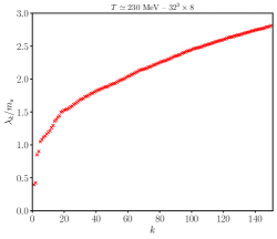
Figure 1: Eigenvalues $\lambda_{k}/m_{s}$ of the staggered operator in the background of a typical gauge configuration on a $32^{3}\times 8$ lattice at $T=230\,\mathrm{MeV}$.

For each gauge configuration we then analyzed the lowest 150 positive eigenvalues of $D^{\mathrm{stag}}[U^{(2)}]$ [i.e., the same operator appearing in the fermionic determinant, Eq. (17)], obtained in Ref. [66] using the PARPACK library [86], from which we computed the corresponding unfolded eigenvalues. We complemented these data by performing a new calculation to obtain the IPRs of the Dirac eigenvectors for the gauge ensembles with $N_{t}=14$. An example of a staggered Dirac spectrum on a single, typical configuration is shown in Fig. 1. We performed unfolding by ordering all the available eigenvalues $\lambda_{n}$ of all the configurations of a given lattice ensemble, and replacing them with their rank divided by the number of configurations [17]. This automatically yields unit spectral density, while the deviation of $\langle s\rangle$ from 1 can be used to test the accuracy of the procedure.

To compute $I_{s_{0}}$ and $\mathrm{Var}(s)$ locally in the spectrum we approximated Eq. (10) by binning the spectrum in bins of size $0.178m_{s}$ in physical units, averaging inside each bin, and assigning the result to the center of the bin. Since, loosely speaking, the Dirac spectrum renormalizes like the quark mass [87, 88, 89, 90, 91], keeping the bin size fixed in units of $m_{s}$ is the appropriate choice. An unfolded spacing was included in a bin average if the corresponding lowest (not unfolded) eigenvalue fell in the bin.

We similarly computed $\langle s\rangle$, and found it compatible with 1 within errors in the relevant spectral region $\lambda/m_{s}\geq 1.5$, see Fig. 2. This reassures us on the validity of our unfolding procedure. Between 1 and 1.5 there is a small but significant deviation from 1, systematically increasing as one goes down in $\lambda$. This is well understood [20], and it is due simply to the low but rapidly changing spectral density, that requires the use of large bins to have a decent signal, at the price of having a non-constant density inside the bin. This leads to the smaller eigenvalue spacings corresponding to modes at the higher, and denser, end of the bin, lowering the numerical estimate $\langle\Delta\lambda\rangle_{\mathrm{bin}}$ of the local average spacing between neighboring eigenvalues in a spectral bin below the expected value $1/\rho_{0\,\mathrm{bin}}$, leading to $\langle s\rangle_{\mathrm{bin}}\simeq\langle\Delta\lambda\rangle_{\mathrm{bin}}\,\rho_{0\,\mathrm{bin}}<1$ for the numerical estimate of $\langle s\rangle$. Between 1 and 1.5 one can also see a systematically increasing deviation from 1 as $N_{t}$ increases (see Fig. 2, top panel). This is due to the formation of distinct taste-degenerate multiplets in this spectral region which, being most likely found at the higher end of a spectral bin, are also more likely to spread across neighboring bins. This leads to lowering $\langle\Delta\lambda\rangle_{\mathrm{bin}}$ further, as spacings within a taste multiplet are more likely to contribute than spacings between multiplets. This explanation is supported by the fact that increasing $N_{s}$ at fixed $N_{t}$, so bringing the multiplets closer, reduces the distance of $\langle s\rangle_{\mathrm{bin}}$ from 1, see Fig. 2, bottom panel. Finally, for $\lambda/m_{s}<1$ the spectrum is very sparse, and it is hard to make any reliable statement.

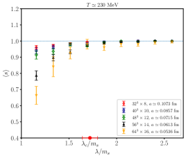
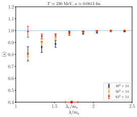
Figure 2: Top panel: comparison of $\langle s\rangle$ as a function of $\lambda/m_{s}$ for all the explored lattice spacings at fixed value of the aspect ratio $LT=4$. Bottom panel: comparison of $\langle s\rangle$ as a function of $\lambda/m_{s}$ for all the explored aspect ratios, corresponding to different values of $N_{s}$, at fixed value of the lattice spacing, corresponding to a temporal extent $N_{t}=14$. Our continuum estimate for the mobility edge (see below Sec. 3.5) is marked in both panels by a red circle on the horizontal axis.

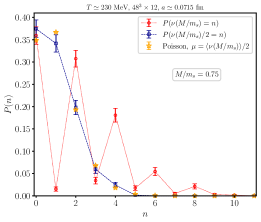
Figure 3: Mode counting in the localized regime of the spectrum. Red circles show the probability $P(\nu(M/m_{s})=n)$ of finding $n$ modes below the cutoff $M=0.75m_{s}$, deep in the localized regime. Blue squares show the probability $P(\nu(M/m_{s})/2=n)$ of finding $n$ mode doublets below the cutoff $M$. Yellow stars show the corresponding Poisson distribution with parameter $\mu=\langle\nu(M/m_{s})/2\rangle$.

3.2 Effects of taste degeneracy on mode countings

As a preliminary piece of evidence of the strong effects of taste degeneracy on the statistical properties of the spectrum, in Fig. 3 we show with red circles the probability distribution of the number $\nu(M/m_{s})$ of eigenmodes found below a fixed cutoff, i.e., $\lambda_{n}\leq M$, with $M$ chosen safely below the mobility edge (see below Sec. 3.5). Notice that $\nu$ is a renormalized quantity if the renormalized physical value of $M$ is kept fixed [87, 88, 89, 90, 91], e.g., if $M/m_{s}$ is kept fixed. While the expectation is that this counting follows a Poisson distribution with parameter equal to the average number of modes below the cutoff, $\langle\nu(M/m_{s})\rangle$, the data show otherwise.

Quite striking at first sight is the oscillating behavior that leaves the odd bins almost empty. This, however, is easily understood if we take notice that the low-lying spectrum shows the formation of eigenvalue doublets (see Fig. 1), the first step in the formation of the quartets expected in the continuum limit (see, e.g., Ref. [92]). If we correct for this by counting the number of doublets, $\nu/2$, instead of the number of modes, and compare with the Poisson distribution with parameter equal to the average number of doublets (i.e., half the average number of modes) below the cutoff, then we find excellent agreement between the two curves, shown with blue squares and yellow triangles in Fig. 3.

This is a simple but convincing demonstration that spectral statistics are heavily distorted by taste-degeneracy effects on fine lattices. It also shows that the taste doublets of eigenmodes fluctuate independently, as expected for localized modes in the absence of near-degeneracy. We now proceed with a quantitative assessment of these effects on the unfolded level spacing distribution.

3.3 Determination of the mobility edge from spectral statistics

We estimated the mobility edge using spectral statistics as the point where these match their critical behavior using two features of the unfolded level spacing distribution, namely $I_{s_{0}}$ and $\mathrm{Var}(s)$. For $I_{s_{0}}$, the critical value was obtained in Ref. [5] by means of a finite-size-scaling analysis, and reads

$$I_{s_{0},c}=0.1966(25)\,.$$ (18)

Here we determined the critical value of $\mathrm{Var}(s)$ by means of a similar analysis on the same lattice data ($2+1$ QCD at $T\simeq 2.6T_{c}$, $a\simeq 0.125\,\mathrm{fm}$, physical $m_{l,s}$): technical details about the procedure can be found in Ref. [5]. Our estimate is

$$\mathrm{Var}(s)_{c}=0.3702(98)\,.$$ (19)

The central value is obtained using only lattices of spatial size $N_{s}\geq 40$ and data points in a range of width $a\Delta\lambda=0.026$ around the mobility edge. The error includes the contribution of the statistical error from the fit, performed with the MINUIT routine [93]; the systematic finite-volume effect estimated as the change of the fit result due to including also $N_{s}=36$ data; and the systematic of the fitting range estimated as the change of the fit result due to shifting the fitting range down in the spectrum by $10\%$ of its width.

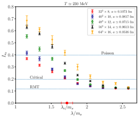
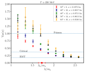
Figure 4: Comparison of $I_{s_{0}}$ (top panel) and $\mathrm{Var}(s)$ (bottom panel), computed locally in the spectrum on lattices at fixed temperature $T=230\,\mathrm{MeV}$, for different values of the lattice spacing at fixed spatial lattice size $L=3.4\,\mathrm{fm}$ in physical units (i.e., fixed $LT=4$). Our continuum estimate for the mobility edge (see below Sec. 3.5) is marked by a red circle on the horizontal axis.

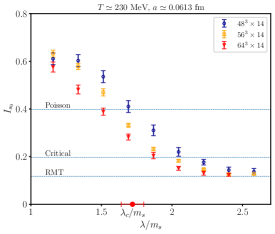
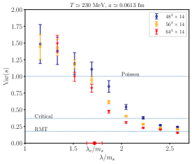
Figure 5: Comparison of $I_{s_{0}}$ (top panel) and $\mathrm{Var}(s)$ (bottom panel), computed locally in the spectrum on lattices at fixed temperature $T=230\,\mathrm{MeV}$, for different spatial volumes at fixed lattice spacing, $a=0.0615\,\mathrm{fm}$ (i.e., $N_{t}=14$). Our continuum estimate for the mobility edge (see below Sec. 3.5) is marked by a red circle on the horizontal axis.

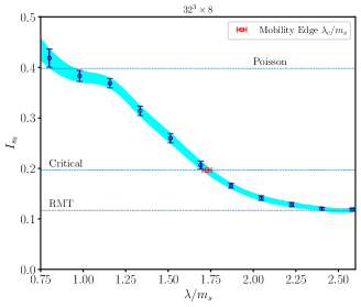
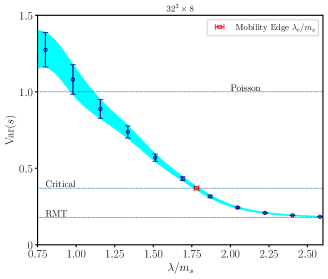
Figure 6: Determination of the mobility edge for our $32^{3}\times 8$ lattice from the dependence of $I_{s_{0}}$ (top panel) and $\mathrm{Var}(s)$ (bottom panel) on the spectral region.

The qualitative behavior of the dependence of $\lambda_{c}^{\mathrm{stat}}/m_{s}$ on the lattice spacing at fixed aspect ratio can be easily deduced from Fig. 4: as $a\to 0$, both $I_{s_{0}}$ and $\mathrm{Var}(s)$ tend to increase throughout the spectrum, as expected, leading to a larger estimate for the mobility edge. In particular, $I_{s_{0}}$ overshoots the Poisson expectation at the low end of the spectrum already on our coarsest lattices (even on the $32^{3}\times 8$, where this happens outside of the spectral window displayed in the plot), showing that taste degeneracy is already distorting the spectral statistics there. While this is not a problem as it does not affect the region where the mobility edge actually is (see below Sec. 3.5), as the lattice becomes finer $I_{s_{0}}$ also overshoots its RMT expectation deeper in the bulk of the spectrum, signaling that the effects of taste multiplets on spectral statistics become important there, too.

The data show that the two coarsest lattices ($N_{t}=8,10$) give compatible results for the spectral statistics in all spectral regions in the bulk of the spectrum, and down to the first bin below the mobility edge. Barring a conspiracy, this indicates two things: that the formation of taste multiplets does not have significant effects in that spectral region yet; and that, when this is the case, further lattice artifacts, on top of those introduced by taste-degenerate multiplets, are small when considering localization properties at fixed physical volume. This shows that the determination of the mobility edge from the critical spectral statistics is reliable on these lattices. Clearly, it may still be affected by finite-volume systematics, but these would involve only effects unrelated to taste multiplets (such as the localization length in certain spectral regions near the mobility edge being too large compared with the spatial size of the system), which are expected not to affect much the determination of the mobility edge via the matching with the critical statistics (see above in Sec. 2.3).

The dependence of $\lambda_{c}^{\mathrm{stat}}/m_{s}$ on the aspect ratio at fixed lattice spacing is visible instead in Fig. 5, where $N_{t}=14$ and the spatial size is varied. Here a larger aspect ratio drives $I_{s_{0}}$ and $\mathrm{Var}(s)$ down, as expected, so leading to an estimate for the mobility edge that decreases with the spatial volume. Notice that the scale-invariant nature of the mobility edge is still masked here by the distortions of the unfolded level spacing distribution, and no volume-independent crossing point of the various curves is present. This shows that the effects of taste degeneracy are still strong even on our largest lattice at $N_{t}=14$. This is in agreement with the argument discussed in Sec. 2.4, as, according to Eq. (15), we would need an aspect ratio of $LT\sim 9$ at this lattice spacing in order to have the same $\delta/\Delta$ that we have for $N_{t}=8$ with $LT=4$.

In order to estimate $\lambda_{c}^{\mathrm{stat}}/m_{s}$ quantitatively, we interpolated our numerical results for $I_{s_{0}}$ and $\mathrm{Var}(s)$ with splines, defining an uncertainty band by interpolating the central values augmented or reduced by the error. We then determined $\lambda_{c}^{\mathrm{stat}}/m_{s}$ as the center of the interval where the band crosses the critical value, and the corresponding error as the half-width of this interval. This procedure is visualized in Fig. 6 for our $32^{3}\times 8$ lattice. Our final results are summarized in Tab. 2.

$T=230$ MeV, $\quad T/T_{c}=1.48$
$N_{s}$	$N_{t}$	$N_{s}/N_{t}$	$\lambda_{c}/m_{s}$ (From $I_{s_{0}}$)	$\lambda_{c}/m_{s}$ (From $\mathrm{Var}(s)$)
32	8	4	1.727(26)	1.780(15)
40	10	4	1.742(30)	1.817(12)
48	12	4	1.865(23)	1.979(21)
48	14	3.4	2.124(61)	2.235(26)
56		4	1.985(27)	2.088(13)
64		4.6	1.889(36)	1.955(20)
64	16	4	2.112(43)	2.199(39)

Table 2: Summary of our results for the mobility edge in units of the strange quark mass, obtained by matching the behavior of the spectral statistics with the expected critical behavior.

3.4 Taste-degeneracy effects on the mobility edge in the thermodynamic limit

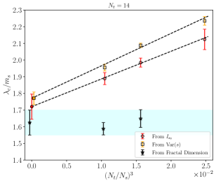
Figure 7: Dependence of our estimates for the mobility edge on the spatial size of the lattice, at fixed temporal extension $N_{t}=14$. The dashed lines represent thermodynamic extrapolations of $\lambda_{c}^{\mathrm{stat}}/m_{s}$ assuming leading linear corrections in the inverse spatial volume $(N_{t}/N_{s})^{3}=1/(LT)^{3}$. The filled points at zero are the results of our extrapolations. Empty and filled starred points, and the shaded area, are our estimates of the mobility edge from the fractal dimension, see text for more details. Points have been slightly shifted horizontally to improve readability.

In order to show that the effects of taste degeneracy become irrelevant for the determination of the mobility edge with our method when taking the thermodynamic limit at fixed lattice spacing, we have compared the $N_{s}\to\infty$ extrapolation of our $N_{t}=14$ data with an independent determination of $\lambda_{c}$ based directly on the properties of the eigenvectors. The infinite-volume extrapolation is shown in Fig. 7; the corresponding results for the mobility edge are:

$$\frac{\lambda_{c}}{m_{s}} =1.721(76),\qquad (\text{from }I_{s_{0}}),$$ (20)

$$\frac{\lambda_{c}}{m_{s}} =1.771(37),\qquad (\text{from }\mathrm{Var}(s)).$$ (21)

To determine $\lambda_{c}$ directly from the eigenvectors, we estimated the local fractal dimension numerically as

$$\alpha_{\mathrm{num}}(\lambda)=3+\frac{\log\left(\overline{\mathrm{PR}}(\lambda,N_{s2})/\overline{\mathrm{PR}}(\lambda,N_{s1})\right)}{\log(N_{s2}/N_{s1})}\,.$$ (22)

Our results are shown in Fig. 8. We then looked for the point in the spectrum where $\alpha_{\mathrm{num}}$ takes its critical value $\alpha_{*}=1.173_{-26}^{+32}$ [55], using a spline interpolation of the numerical data. This is visualized in Fig. 9. To quote a final value, we considered the results obtained with the pairs $(N_{s1},N_{s2})=(48,56)$ and $(48,64)$, and took as our final estimate a symmetric confidence band including both error bars. The two values are compatible within errors (see Fig. 7), showing that finite-size effects on this estimate of the mobility edge are reasonably small. As a further check, we verified that the pair $(N_{s1},N_{s2})=(56,64)$ gave compatible results, although within much larger statistical errors. In the end, we obtain:

$$\frac{\lambda_{c}}{m_{s}}=1.625(75),\quad\,(\text{from fractal dimension}).$$ (23)

This is in good agreement with the thermodynamic extrapolation of our estimates from spectral statistics, Eq. (20), see Fig. 7. This shows that these are indeed converging to the actual position of the mobility edge. Moreover, this further confirms that finite-size effects on the estimate based on the critical fractal dimension are reasonably small.

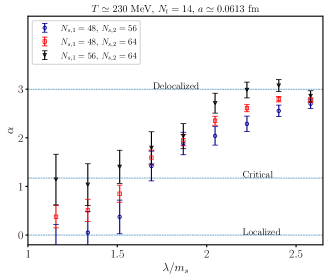
Figure 8: Behavior of the fractal dimension as a function of the spectral bin computed for $N_{t}=14$ for several choices of the lattice sizes $N_{s,1}$ and $N_{s,2}$.

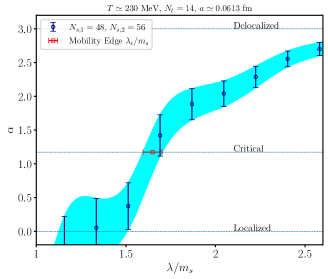
Figure 9: Determination of the mobility edge from the fractal dimension of eigenmodes, estimated using results from $48^{3}\times 14$ and $56^{3}\times 14$ lattices [see Eq. (22)].

3.5 Dependence of the mobility edge on the lattice spacing

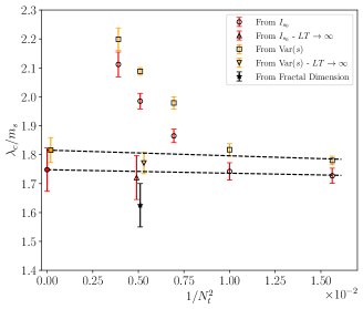
Figure 10: Dependence of our estimates for the renormalized mobility edge as a function of the lattice spacing at fixed temperature $T=230\,\mathrm{MeV}$. The dashed lines represent continuum extrapolations of $\lambda_{c}/m_{s}$ assuming leading linear corrections in $(1/N_{t})^{2}=(aT)^{2}$, see text for details. Points have been slightly shifted horizontally to improve readability.

We finally summarize the results of the previous two subsections in Fig. 10, showing together all our determinations of $\lambda_{c}/m_{s}$. It is clear that our two coarsest lattice give compatible estimates via $\lambda_{c}^{\mathrm{stat}}/m_{s}$, while on finer lattices with the same aspect ratio these estimates rapidly deviate. On the other hand, the infinite-volume extrapolation at $N_{t}=14$ gives again results compatible with our coarsest lattices, as well as with the determination from the local fractal dimension.

Before attempting an extrapolation of $\lambda_{c}/m_{s}$ to the continuum, it is important to discuss whether the order in which one takes the thermodynamic and continuum limits matters. In this context, our estimate based on $\alpha(\lambda)$, being unaffected by taste degeneracy, allows us to define a valid estimate of the position of the mobility edge at both finite aspect ratio and finite spacing. Our numerical results show that this quantity does not depend strongly on the aspect ratios employed. Moreover, our results obtained at $N_{t}=14$ are not very different from the estimates obtained using spectral statistics on our coarsest lattices $N_{t}=8,10$, where taste-degeneracy effects are negligible and estimates based on critical statistics should accurately reflect the position of the mobility edge in the thermodynamic limit. These observations suggest that the estimate of the mobility edge based on the fractal dimension does not depend strongly neither on the aspect ratios nor on the lattice spacing. There is therefore no reason to expect the continuum and thermodynamic limit not to commute, when measuring the position of the mobility edge directly from the eigenvectors. Thus, since the thermodynamic limit of this estimate at fixed spacing matches that of the estimate from spectral statistics, we expect that taking the thermodynamic limit followed by the continuum limit of the latter provides the correct value of the mobility edge in the continuum theory.

In the light of this discussion, we have performed an extrapolation to the continuum limit using our estimates of $\lambda_{c}/m_{s}$ from spectral statistics for $N_{t}=8,10$ and $N_{t}=14$, where for $N_{t}=14$ we have used the results extrapolated first towards the thermodynamic limit. The results obtained from the two observables $I_{s_{0}}$ and $\mathrm{Var}(s)$ are:

$$\frac{\lambda_{c}}{m_{s}} =1.748(75),\qquad (\text{from }I_{s_{0}}),$$ (24)

$$\frac{\lambda_{c}}{m_{s}} =1.816(43),\qquad (\text{from }\mathrm{Var}(s)),$$ (25)

perfectly compatible within errors. To our knowledge, this result is the first fully controlled extrapolation of $\lambda_{c}/m_{s}$ to the continuum.

4 Conclusions

Localization of the low-lying Dirac eigenmodes in the high-temperature phase of QCD and other gauge theories [3, 4, 5, 6, 7, 8, 9, 10, 11, 12, 13, 14, 15, 16, 17, 18, 19, 20, 21, 22, 23, 24, 25, 26, 27, 28, 29, 30] is closely related to the change in the confining properties of these theories [18, 32, 33, 34, 12, 26, 19, 20, 21, 22, 25, 26, 28, 29], and its study can lead to a better understanding of the mechanism behind deconfinement, and its relation with chiral symmetry restoration.

The strong connection between deconfinement and localization is exemplified by the fact that the mobility edge, i.e., the point in the spectrum separating localized and delocalized modes in the spectrum, decreases as one approaches the pseudocritical temperature from above, and vanishes in the crossover range. In theories with a genuine deconfinement transition, this takes place exactly at the critical point [19, 20, 21, 22, 25, 26, 28, 29]. A more accurate quantitative determination of the “geometric” transition temperature where the mobility edge vanishes and localization disappears, and so of the tightness of the connection between localization and deconfinement, requires the full control of systematic effects, including finite volume and, especially, finite spacing effects.

Most of the numerical studies of localization combine the relation between the localization properties of eigenmodes and the statistical properties of the corresponding eigenvalues [36] with the use of the staggered discretization of the Dirac operator [3, 4, 5, 7, 22, 29, 17, 18, 19, 20, 25, 26, 28, 30]. However, this approach faces serious technical problems due to the restoration of taste symmetry in the continuum limit: as the lattice becomes finer the spectrum tends to organize in nearly-degenerate multiplets of eigenmodes, which in turn distort the spectral statistics away from their expected universal behavior, leading to hard-to-control systematic effects in the determination of the mobility edge.

In this paper we have carried out a dedicated study of the effects of taste degeneracy on the statistical properties of the staggered spectrum in high-temperature lattice QCD. We focused in particular on how these affect the numerical determination of the mobility edge, and how these effects change as the lattice spacing is reduced, or the aspect ratio is increased, with the main goal of providing a controlled continuum limit of the mobility edge.

Our findings are in line with theoretical expectations, with a systematic overestimation of the mobility edge on finer lattices, where the effects of taste degeneracy become sizeable also in the bulk of the spectrum. For larger aspect ratios at fixed lattice spacing these effects are reduced and the overestimation of the mobility edge is mitigated. In the thermodynamic limit, this estimate tends to the correct value of the mobility edge, obtained independently by studying the fractal dimension of the eigenvectors. Moreover, this quantity shows a mild dependence on both volume and lattice spacing, suggesting the interchangeability of the continuum and thermodynamic limits.

The most important result of this analysis is that the infinite-volume extrapolation of the mobility edge on a finer lattice is in good agreement with the mobility edge found on coarser lattices, where taste-degeneracy effects do not reach into the bulk of the spectrum and a reliable estimate can be obtained from spectral statistics already at lower aspect ratios. This shows that accurate values for the mobility edge can be obtained on relatively coarse lattices for reasonable aspect ratios using spectral statistics, which is the ideal combination from the numerical point of view.

Moreover, our findings allowed us to perform the first, fully controlled extrapolation of the mobility edge to the continuum limit. This confirms the theoretical expectation [4, 35] that the mobility edge in units of the quark mass is a renormalized quantity with physical meaning, and not only a lattice artifact. It also lends support to the numerical evidence for this fact presented in Refs. [4, 29]. There it was shown that the mobility edge depends only mildly on the lattice spacing. In the light of our results, this is because the calculations of Refs. [4, 29] use relatively coarse lattices, where taste-degeneracy effects on the mobility edge are negligible. One might have wondered if the situation could have changed on finer lattices; our results show that this mild dependence would still show on finer lattices, provided one extrapolated first to the thermodynamic limit. (Incidentally, the extrapolation in $T$ shown in Ref. [4] is in good qualitative agreement with our result.)

In conclusion, we have shown that one can use staggered fermions efficiently and reliably to study the mobility edge in the Dirac spectrum of high-temperature lattice gauge theories, provided that the aspect ratio is sufficiently large to avoid sizeable taste-degeneracy effects in the relevant region of the spectrum. Moreover, we have numerically demonstrated that the mobility edge in units of the quark mass is a renormalized quantity, in agreement with theoretical expectations; and that it depends only mildly on the lattice spacing.

It would be interesting to understand if and how one could avoid the well known problems of the staggered discretization (i.e., lack of good chiral properties, difficult relation with topology) by relating the staggered and the overlap spectrum on the same gauge configurations. In this context, the mobility edge could be used in two different ways. On the one hand, renormalizing the overlap spectrum (after matching a suitable observable to find the renormalization constant) would allow one to obtain another estimate for $\lambda_{c}/m_{s}$ from spectral statistics unaffected by taste degeneracy, to be compared with the one obtained here after extrapolating to infinite volume. On the other hand, thanks to its mild dependence on the lattice spacing the mobility edge itself could be efficiently used to match the staggered and overlap spectra.