GRB 231115A: a nearby Magnetar Giant Flare or a cosmic Short Gamma-Ray Burst?

Abstract

There are two classes of gamma-ray transients with a duration shorter than 2 seconds. One consists of cosmic short Gamma-Ray Bursts (GRBs) taking place in the deep universe via the neutron star mergers, and the other is the magnetar giant flares (GFs) with energies of $\sim 10^{44}-10^{46}$ erg from “nearby” galaxies. Though the magnetar GFs and the short GRBs have rather similar temporal and spectral properties, their energies ($E_{\rm\gamma,iso}$) are different by quite a few orders of magnitude and hence can be distinguished supposing the host galaxies have been robustly identified. The newly observed GRB 231115A has been widely discussed as a new GF event for its high probability of being associated with M82. Here we conduct a detailed analysis of its prompt emission observed by Fermi-GBM, and compare the parameters with existing observations. The prompt gamma-ray radiation properties of GRB 231115A, if associated with M82, nicely follow the $E_{\rm p,z}$–$E_{\gamma,\rm iso}$ relation of the GFs, where $E_{\rm p,z}$ is the peak energy of the gamma-ray spectrum after the redshift ($z$) correction. To be a short GRB, the reshift needs to be $\sim 1$. Though such a chance is low, the available X-ray/GeV observation upper limits are not stringent enough to further rule out this possibility. We have also discussed the prospect of convincingly establishing the magnetar origin of GRB 231115A-like events in the future.

1 Introduction

Gamma-ray Bursts (GRBs) have been observed for over half a century, and can be classified into short GRBs and long GRBs based on their bimodal duration distribution (Kouveliotou et al., 1993). Long GRBs typically originate in star-forming regions within galaxies and are observed in association with massive star-collapse supernovae (Woosley, 1993; Fruchter et al., 2006), while short GRBs are found in low star-forming regions of their host galaxies and are believed to originate from compact binaries (Eichler et al., 1996; Narayan et al., 1992; Gehrels et al., 2005; Fong et al., 2010; Leibler & Berger, 2010; Fong & Berger, 2013; Berger, 2014). In addition, there are notable distinct events called giant flares (GFs) emitting from magnetars, which exhibit characteristics similar to those of short GRBs and are mixed in with the current observations (Duncan, 2001; Hurley et al., 2005; Lazzati et al., 2005; Popov & Stern, 2006). When the burst is associated with a Soft Gamma-ray Repeater (SGR) or when the host galaxy is identified, several events are revealed. These include GRBs 790305 (SGR 0526-66; Mazets et al. 1979, 1982), 980618 (SGR 1627-41; Mazets et al. 1999a; Woods et al. 1999; Aptekar et al. 2001), 980827 (SGR 1900+14; Hurley et al. 1999; Mazets et al. 1999b; Tanaka et al. 2007), and 041227 (SGR 1806-20; Hurley et al. 2005; Palmer et al. 2005; Frederiks et al. 2007a), which are associated with SGRs. Additionally, GRBs 051103 (M81; Frederiks et al. 2007b), 070201 (M31; Mazets et al. 2008a), 070222 (M83; Burns et al. 2021), and 200415A (NGC 253; Roberts et al. 2021; Svinkin et al. 2021; Yang et al. 2020; Zhang et al. 2020) are likely associated with specific galaxies.

The common characteristics of observed GFs include the rapidly rising exponential decay light curves, the hard and rapidly evolving energy spectra, and the high energies of $10^{44}-10^{46}$ erg (Hurley et al., 1999; Mazets et al., 1999b; Frederiks et al., 2007a). GRB 980618, the most intense flare observed from the SGR 1626-41, shows a distinct characteristic which is a relatively slow-rise light curve (Mazets et al., 1999a). However, what can be considered as a “smoking gun” evidence is the presence of long periodic tails after initial pulses (Mazets et al., 1979; Hurley et al., 1999, 2005), originating from the modulation of the rotation period of the neutron star (Barat et al., 1983; Israel et al., 2005; Strohmayer & Watts, 2005; Watts & Strohmayer, 2006). When GFs occur in other galaxies, it may only be possible to detect the initial pulses without the presence of periodic tails. Therefore, the identification of such events is both interesting and challenging.

In this work we focus on GRB 231115A, a new GF candidate detected by Fermi-GBM (Dalessi et al., 2023; Burns, 2023; Minaev et al., 2023; Frederiks et al., 2023). Our work is organized as follows. In Section 2, we provide a summary of current observations and conduct a detailed analysis of Fermi-GBM observation data, along with the observational upper limit of Fermi-LAT. In Section 3, we present various characteristics of the prompt emission and compare them with known GRBs and GFs. In Section 4, we model the multi-band light curves under each scenario and derive possible constraints on the age of the magnetar within the GF scenario. Finally, in Section 5, we summarize all features and discuss potential opportunities for known facility observations.

2 Observersion and data analysis

At 15:36:21 UT on November 15, 2023, GRB 231115A triggered Fermi-GBM. The position coordinates were RA = 131.0, Dec = 73.5 with the statistical uncertainty 8 degrees (Fermi GBM Team, 2023). INTEGRAL (Mereghetti et al., 2023) have reported more accurate position uncertainty (2 arcmin) and is consistent with the M82 galaxy (coincidence probability $\sim$ 0.03%), marked with red “+” (RA = 149.0, Dec = 69.7) in Figure 1. There have no exact multi-messenger counterparts including radio (Curtin & Chime/Frb Collaboration, 2023), optical (Kumar et al., 2023; Hu et al., 2023), X-ray (Kong & Li, 2023; Osborne et al., 2023; Rigoselli et al., 2023), neutrino (IceCube Collaboration, 2023) and gravitational waves (Ligo Scientific Collaboration et al., 2023). The positions of possible optical transients sources are marked with small red circles as shown in Figure 1.

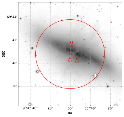
Figure 1: The ZTF r-band image of M82 field. The large red circle with a “+” at its center shows the localization from INTEGRAL (Mereghetti et al., 2023). Three small red circles marked with S1, S2 and S3 represent the position of possible transient AT2023xvj (Kumar et al., 2023), W20231115a and W20231115b (Hu et al., 2023).

Therefore, we mainly focus on what information the Fermi-GBM observations can bring to us, and further data analysis is completed by HEtools (Wang et al., 2023). The instrumentation of the Fermi-GBM payload encompasses two types of detectors: specifically, 12 sodium iodide (NaI) detectors and 2 bismuth germanate (BGO) detectors (Meegan et al., 2009). Based on the location of the source and the orientation of the instrument, we selected a NaI (n7) detector and a BGO (b1) detector respectively. For such extremely short-duration events, we use Time-Tagged Event (TTE) data for analysis to ensure sufficiently high temporal resolution. Light curves and energy channels recorded for photons from 50–300 keV are shown in the top two panels of Figure 2. A total of four episodes for spectral analysis, corresponding to a ($T_{0}+[-0.018,~{}-0.007]~{}\rm s$), b ($T_{0}+[-0.007,~{}0.001]~{}\rm s$), c ($T_{0}+[0.001,~{}0.044]~{}\rm s$), and integrated period ($T_{0}+[-0.018,~{}-0.044]~{}\rm s$). Based on the accumulated percentage of photon events (Koshut et al., 1996), we calculated $T_{90}$ ($\sim$ 46 ms) of 50–300 keV energy range, which is shown in the third panel of Figure 2.

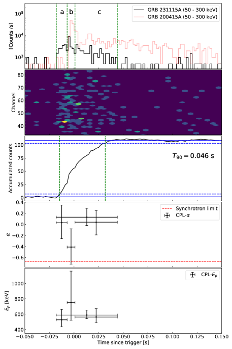
Figure 2: Observation data of Fermi-GBM and parameter evolution of CPL model. The first panel shows the light curves of GRB 231115A and GRB 200415A in the 50-300 keV energy range, and the time period used for spectral analysis. The second panel shows the count corresponding to channel. The third panel is the photon count accumulation curve and duration from 5% to 95%. The two bottom panels are the evolution of the spectral index $\alpha$ and energy peak $E_{p}$ of the CPL model, where the red dotted line represents the synchrotron limit.

2.1 Spectral Analysis of Fermi-GBM

By using GBM Data Tools (Goldstein et al., 2021) we extracted the spectrum files, background files, response files for the four episodes mentioned above, and determined the model parameters of the photon spectrum through forward fitting method. Here we consider two types of photon spectral models. The first is the cutoff power-law (CPL) model usually used to describe the GRB spectrum, written as

$${N(E)=A\left(\frac{E}{100\,{\rm keV}}\right)^{\alpha}\exp\left(-\frac{E}{E_{\rm c}}\right)},$$ (1)

where $\alpha$ is the power law photon spectral index, E_c is the break energy in the spectrum, and the peak energy $E_{\rm p}$ is equal to $E_{\rm c}(2+\alpha)$. Since the spectrum of GF is usually quasi thermal, another type of model is the single blackbody (BB) model and the multicolor blackbody (mBB) model. The BB model is expressed as

$${N(E)=\frac{8.0525\times KE^{2}}{(kT)^{4}(e^{E/kT}-1)}}$$ (2)

where kT is the blackbody temperature keV; K is the L₃₉/ D${}_{10}^{2}$, where L₃₉ is the source luminosity in units of 10³⁹ erg/s and D₁₀ is the distance to the source in units of 10 kpc. And the multicolor blackbody (mBB) model (Ryde et al., 2010; Hou et al., 2018) is expressed as

$$N(E)=\frac{8.0525(m+1)K}{\left[\left(\frac{T_{\max}}{T_{\min}}\right)^{m+1}-1\right]}\left(\frac{kT_{\min}}{\rm keV}\right)^{-2}I(E),$$ (3)

where

$$I(E)=\left(\frac{E}{kT_{\rm min}}\right)^{m-1}\int_{\frac{E}{kT_{\rm max}}}^{\frac{E}{kT_{\rm min}}}\frac{x^{2-m}}{e^{x}-1}dx,$$ (4)

where $x=E/kT$, the temperature range from $kT_{\rm min}$ to $kT_{\rm max}$, and the index $m$ of the temperature determines the shape of spectra. Then Bayesian inference methods (Thrane & Talbot, 2019; van de Schoot et al., 2021) was used for parameter estimation and comparison of photon spectrum models. In our analysis, PyMultiNest (Buchner et al., 2014) with Bilby (Ashton et al., 2019) package is used for the bayesian inference. For GBM data, the likelihood function used is pgstat, refer to the XSPEC manual. The original intention of nest sampling is to provide evidence of the model,and the model selection can be done by comparing Bayes factors. And the Bayes factor (BF) is the ratio of the Bayesian evidence ($\mathcal{Z}=\int\mathcal{L}(d|\theta)\pi(\theta)d\theta$) for different models. The log of Bayes factor can be written as $\ln\text{BF}^{\text{A}}_{\text{B}}=\ln({\cal Z}_{\text{A}})-\ln({\cal Z}_{\text{B}})$. When $\ln{\rm BF}>8$, we can say that there is a “strong evidence” in favor of one hypothesis over the other (Thrane & Talbot, 2019).

The posterior parameters of each model and the results of model selection are shown in Table 1. In Figure 2, the two bottom panels show the evolution over time of the power law photon spectral index ($\alpha$) and the energy peak ($E_{p}$) respectively. It is worth noting that the $\alpha$ of CPL model exceed the synchrotron limit, also known as the “Line of Death” (Preece et al., 1998, 2002). Moreover, its spectrum is harder than that of ordinary GRBs, and all interval favour the mBB model. These characteristics indicate that its spectrum is quasi thermal, with the evolving temperature $kT$. The time-integrated $\nu F_{\nu}$ spectrum and posterior parameter contours are shown in Figure 3.

Table 1: Spectral fitting result

Time interval	Model	$\alpha$/$m$	$E_{p}$/$kT$/$kT_{\rm min}$,$kT_{\rm{max}}$	Flux (1-10000 keV)	$\ln{\cal Z}$	Highest evidence
$T_{0}$+ (s)			(keV)	($10^{-5}$ erg $\rm cm^{-2}$ $\rm s^{-1}$)
Time-integrated spectra
[-0.018, 0.044]	CPL	0.16${}_{-0.16}^{+0.15}$	579.01${}_{-38.89}^{+48.35}$	1.36${}_{-0.09}^{+0.10}$	-219.99
	BB	…	124.00${}_{-6.15}^{+6.79}$	1.24${}_{-0.08}^{+0.08}$	-222.11
	mBB	0.10${}_{-0.17}^{+0.23}$	37.10${}_{-6.64}^{+7.14}$, 267.02${}_{-28.21}^{+40.18}$	1.37${}_{-0.10}^{+0.11}$	-211.98	$\checkmark^{*}$
Time-resolved spectra
[-0.018, -0.007]	CPL	-0.20${}_{-0.13}^{+0.10}$	601.16${}_{-71.47}^{+85.53}$	2.31${}_{-0.26}^{+0.30}$	-164.27
	BB	…	118.55${}_{-9.02}^{+10.71}$	2.13${}_{-0.21}^{+0.25}$	-157.99
	mBB	0.20${}_{-0.15}^{+0.22}$	37.02${}_{-11.22}^{+18.88}$, 228.99${}_{-38.70}^{+48.00}$	2.21${}_{-0.23}^{+0.28}$	-156.29	$\checkmark$
[-0.007, 0.001]	CPL	-0.66${}_{-0.12}^{+0.10}$	1221.93${}_{-257.11}^{+371.04}$	4.13${}_{-0.69}^{+0.91}$	-164.79
	BB	…	151.90${}_{-14.87}^{+16.59}$	2.97${}_{-0.37}^{+0.40}$	-166.25
	mBB	0.11${}_{-0.11}^{+0.17}$	23.12${}_{-7.67}^{+11.39}$, 405.50${}_{-81.23}^{+100.64}$	3.46${}_{-0.50}^{+0.54}$	-160.92	$\checkmark$
[0.001, 0.044]	CPL	-0.28${}_{-0.08}^{+0.06}$	691.80${}_{-71.07}^{+106.47}$	0.99${}_{-0.10}^{+0.13}$	-192.64
	BB	…	118.36${}_{-8.88}^{+11.10}$	0.81${}_{-0.08}^{+0.09}$	-183.19
	mBB	-0.04${}_{-0.11}^{+0.16}$	45.82${}_{-8.20}^{+12.70}$, 249.29${}_{-46.84}^{+59.17}$	0.91${}_{-0.10}^{+0.11}$	-179.21	$\checkmark$

Note. — The “…” represents missing parameters of different models. “$\checkmark^{*}$” represents strong evidence, that is, $\ln$BF $>$ 8.

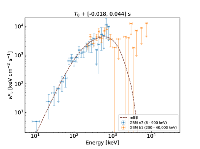
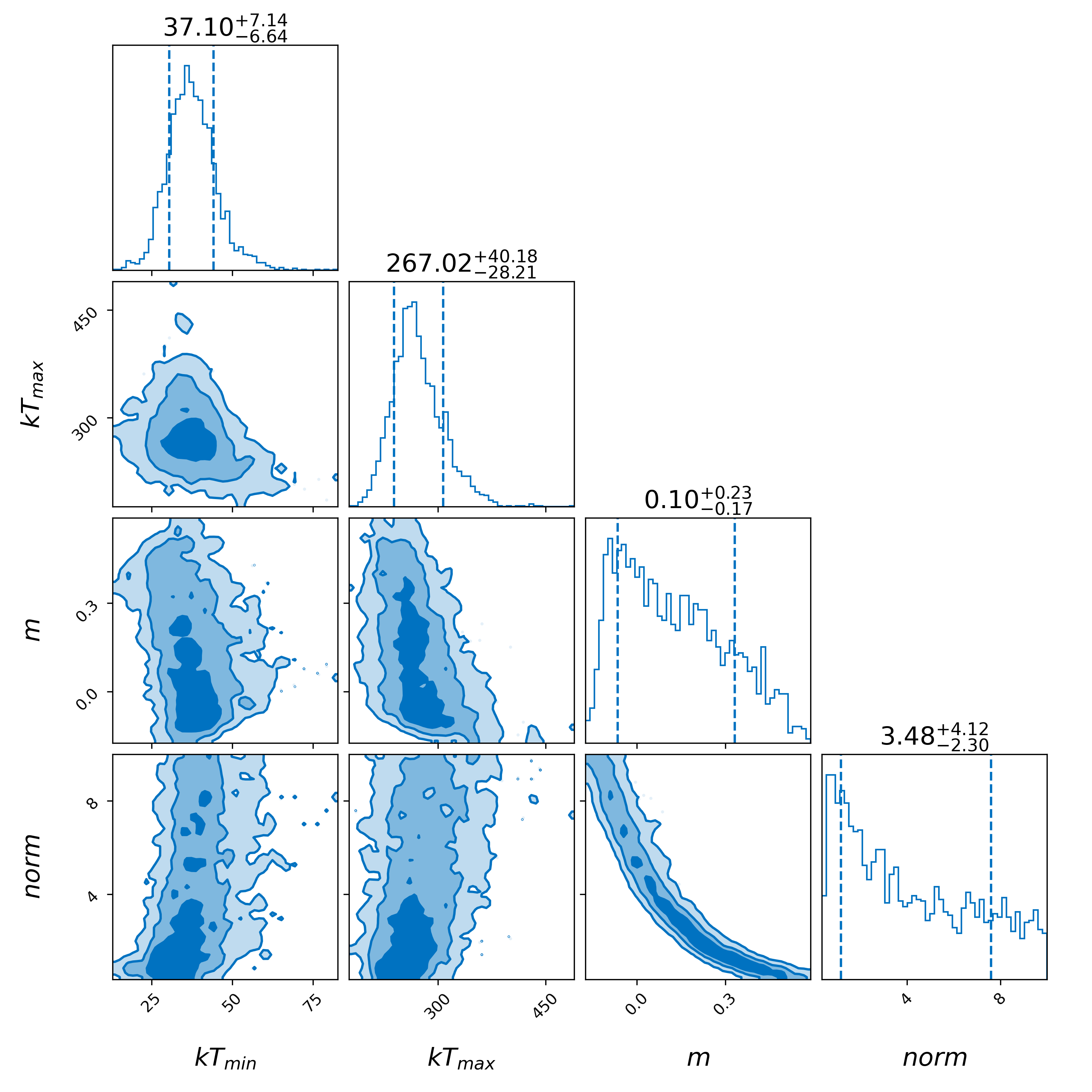
Figure 3: Time-integrated spectra fitting result. Left panel: The $\nu F_{\nu}$ spectra of GRB 231115A at integrated period. Right panel: Posterior contours of mBB model parameters.

2.2 Upper limit of Fermi-LAT

Fermi-LAT is a high performance gamma-ray telescope for the photon energy range from 30 MeV to 1 TeV (Ajello et al., 2021). GRB 231115A has been found in the field of view for Fermi-LAT from ${T_{0}}$ to ${T_{0}}+3000$ s. We select the photon events in the first 3000 s within the energy range from 500 MeV to 5 GeV with the SOURCE event class and the FRONT+BACK type. In order to reduce the contamination from the Earth’s limb, we exclude photons with zenith angles larger than 100^∘. Then we extract good time intervals with the quality-filter cut (DATA_QUAL==1 && LAT_CONFIG==1).

In this work, we use the standard unbinned likelihood analysis within a 10^∘ region of interest (ROI) centered on the INTEGRAL location of GRB 231115A. The initial model for the ROI region, generated by the make4FGLxml.py script, includes the galactic diffuse emission template (gll_iem_v07.fits), the isotropic diffuse spectral model for the SOURCE data (iso_P8R3_SOURCE_V3_v1.txt) and all the Fourth Fermi-LAT source catalog (gll_psc_v31.fit; Abdollahi et al., 2020) sources within 20 degrees around GRB 231115A. We model the $\gamma$-ray emission from the GRB 231115A region as a point source at the INTEGRAL location of (ra, dec) = (149.03^∘, 69.69^∘) and set its spectral shape to the PowerLaw (${\frac{dN}{dE}=N_{0}(\frac{E}{E_{0}})^{\gamma}}$) model with the index of $\gamma=-2$. Due to the very short time interval we select, only normalizations of the galactic, isotropic diffuse models and spectra of GRB 231115A are set to be free parameters in the fitting process. Other parameters are be set as the default of 4FGL. The Fermitools package are used in our work. No significant $\gamma$-ray emission from GRB 231115A was detected by Fermi-LAT. Then a 95$\%$ confidence level upper limit of flux was derived as $1.89\times 10^{-10}\,{\rm erg\,cm^{-2}\,s^{-1}}$ in the energy range of 0.5–5 GeV.

3 CHARACTERISTICS

3.1 Power Density Spectra

We try to find possible periodic signals in the power density spectra (PDS) as it is the strongest evidence for a GF. One of the important step is to model red noise to calculate the significance of periodic frequencies. For the above goal, we used a procedure based on Vaughan (2005, 2010, 2012) and Covino et al. (2019). Also, we refer to Beloborodov et al. (1998); Guidorzi et al. (2012, 2016); Dichiara et al. (2013, 2013) for details on analyzing power density spectra in GRBs. PDS are derived by discrete Fourier transformation and normalized according to Leahy et al. (1983), which fit by a single power-law function plus white noise (Guidorzi et al., 2016),

$$S_{\rm PL}(f)=N\,f^{-\alpha}+B,$$ (5)

here $N$ is a normalization factor, $f$ is the sampling frequency, and its lower limit is related to the length of the time series, which is $1/T$ (the time interval). The upper limit of $f$ is the Nyquist frequency, which is $1/(2{\delta_{t}})$, where $\delta_{t}$ is the time bin size of data. The value of white noise $B$ is expected to be 2, which is the expected value of a $\chi^{2}_{2}$ distribution for pure Poissonian variance in the Leahy normalization.

We also employ a Bayesian inference for parameter estimation by using emcee (Foreman-Mackey et al., 2013). The maximum likelihood function we use is called Whittle likelihood function (Vaughan, 2010). When enough samples are obtained, we calculate the global significance of every frequency in the PDS according to $T_{\rm R}=\max_{j}R_{j}$, where $R=2P/S$, $P$ is the simulated or observed PDS, and $S$ is the best-fit PDS model. This method selects the maximum deviation from the continuum for each simulated PDS. The observed $T_{\rm R}$ values are compared to the simulated distribution and significance is assessed directly. The corrections for the multiple trials performed were included in the analysis because the same procedure was applied to the simulated as well as to the real data. As shown in Figure 4, the PDS exhibits a peak at $\sim$90 Hz, but it is not significant enough to be considered a quasi-periodic signal.

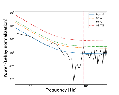
Figure 4: The Power Density Spectra (PDS). The blue solid line represents the best fit of the PDS, while the orange, green, and red dashed lines correspond to significance levels of 90%, 95%, and 99.7%, respectively. The pink dashed line corresponds to the peak of the PDS occurring at $\sim$90 Hz.

3.2 $E_{\rm p,z}$ - $E_{\gamma,\rm iso}$ and EH relation

Through the use of the fitting result of the spectra analysis in Section 2.1 We intended to place GRB 231115A on the $E_{\rm p,z}$ - $E_{\gamma,\rm iso}$ relation(Amati et al., 2002), where $E_{\rm p,z}=(1+z)E_{\rm p}$ is the rest frame peak energy, $E_{\gamma,\rm iso}$ is the isotropic bolometric emission energy, written as

$$E_{\gamma,\text{iso}}=\frac{4\pi d_{L}^{2}kS_{\gamma}}{1+z},$$ (6)

where $d_{L}$ is the luminosity distance, $S_{\gamma}$ is the energy fluence in the gamma-ray band, and $k$ is the correction factor, which can correct the energy range of the observer frame to the energy range of 1–10,000 keV in the rest frame. The correction factor $k$ (Bloom et al., 2001) writes as

$$k=\frac{\int_{1/(1+z)}^{10^{4}/(1+z)}EN(E){\rm d}E}{\int_{e_{1}}^{e_{2}}EN(E){\rm d}E},$$ (7)

where $e_{1}$ and $e_{2}$ correspond to the energy range of the detector. In our calculations, the cosmological parameters of H₀ = $\rm 69.6~{}kms^{-1}~{}Mpc^{-1}$, $\Omega_{\rm m}=0.29$, and $\Omega_{\rm\Lambda}=0.71$. As shown in of Figure 5(a), the solid black line represents the calculation result of redshift from 0.0001 to 5. Obviously, when the luminosity distance of GRB 231115A is 3.5 Mpc (that is, located in the M82 galaxy), it falls within the region of GFs. When it falls within the short GRB region, its redshift is 0.1, marked as a black square on the figure. In addition, we also calculated the results when taking the typical redshift of short GRB ($z=1$), marked as a blue triangle. Additionally, Minaev & Pozanenko (2020a) proposed a new classification scheme combining the correlation of $E_{\gamma,{\rm iso}}$ and $E_{p,z}$ and the bimodal distribution of $T_{90}$. This characteristic parameter $EH$ is written as

$$EH=\dfrac{(E_{p,z}/100{\rm keV})}{(E_{\gamma,iso}/10^{52}{\rm erg})^{0.4}}.$$ (8)

As shown in Figure 5(b), the solid black line also represents the calculation results of the same redshift in $E_{{\rm p},z}$–$E_{\gamma,\rm iso}$ diagram. As the luminosity distance increases, GRB 231115A moves from the region of GFs to the region of short GRBs. And a summary of GRB 231115A and other known GFs is shown in Table 2.

Table 2: Summary of characteristics of know GFs

GF event date	790305	960618	980827	041227	051103	070201	070222	200415	231115
Origin
SGR or Host galaxy	SGR 0526-66	SGR 1627-41	SGR 1900+14	SGR 1806-20	M81	M31	M83	NGC 253	M82
Luminosity Distance (Mpc)	0.050	0.011	0.013	0.0087	3.6	0.74	4.5	3.5	3.5
Prompt characteristics
Duration (s)	$\lesssim 0.25$	$\sim 0.6$	$<$1.0	$<0.2$	0.17	0.01	0.038	0.1	0.046
$E_{p}$ (keV)	$\sim 500$	$\sim 150$	$>250$	$\sim 850$	$\sim 900$	$\sim 300$	$\sim 1300$	$\sim 1100$	$\sim 600$
$E_{\gamma,\rm iso}$ ($10^{45}$ erg)	0.7	0.01	0.43	23	70	1.5	6.2	13	1.3

3.3 Hardness Ratio

The Hardness Ratio (HR) of a GRB is usually expressed as the ratio of photon counts in two fixed energy bands. In addition to the bimodal distribution of $T_{90}$ (Kouveliotou et al., 1993), short GRBs are usually harder than long GRBs (Horváth et al., 2006). Here we calculate the ratio of the observed counts in 50–300 keV compared to the counts in the 10–50 keV band in $T_{0}+[-0.018,~{}0.044]~{}\rm s$. The calculated HR = 8.96, compared with the previous statistical data (Goldstein et al., 2017), is shown in Figure 5(c).

3.4 Spectral Lag

The spectral lag of GRB is that the high-energy photons arrive earlier than the low-energy photons(Norris et al., 2000; Norris, 2002; Norris et al., 2004). The time delay in different energy bands can be quantified using the cross-correlation function (CCF), which is widely used in the calculation of the GRB spectral lag (Band, 1997; Ukwatta et al., 2010). In general, long GRB exhibit a relatively significant spectral delay (Norris et al., 2000; Gehrels et al., 2006), but not for short GRBs (Norris & Bonnell, 2006). Besides, a fraction of short GRBs even show negative lags (Yi et al., 2006). We calculated the CCF of the GRB 231115A time series in the energy band 100-150 keV and 200-250 keV with $T_{0}+[-0.050,~{}0.0150]~{}\rm s$. And we estimated the uncertainty of the lag by Monte Carlo simulation (Ukwatta et al., 2010). The corresponding spectral lags of GRB 231115A is $\tau_{a}=-6.47\pm 11.52~{}\rm{ms}$ as shown in Figure 5 (d). This tiny spectral lag makes GRB 231115A consistent with short GRBs and GF case 200415A (Yang et al., 2020).

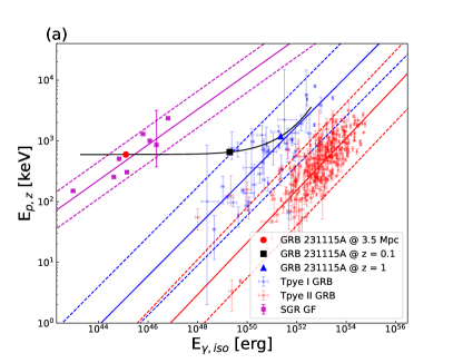
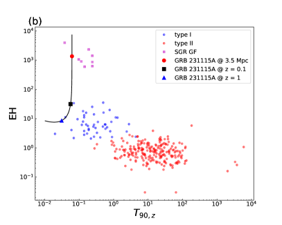
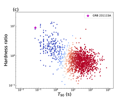
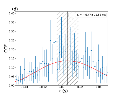
Figure 5: Comparison of GRB 231115A characteristics with other GRBs. (a) is the $E_{\rm p,z}$ - $E_{\gamma,\rm iso}$ diagram. The light blue and light red points are the data of Type I and Type II GRBs with known redshifts, and the corresponding dashed lines represent the 2$\sigma_{\rm cor}$ correlation regions, respectively (Minaev & Pozanenko, 2020a, b). The black trajectory represents the calculation of redshift from 0.0001 to 5. The red points, black squares and blue triangles are the results of GRB 231115A at 3.5 Mpc, z=0.1 and z=1 respectively. (b) is the EH relation, and the colors and labels are the same as in (a). (c) is the hardness ratio of known GRBs (Goldstein et al., 2017), in which the purple star represents GRB 231115A. (d) is the spectral lags result, and the error comes from the Monte Carlo simulation of the light curve (Ukwatta et al., 2010).

3.5 Initial Lorentz factor

For such large energy ($\sim 10^{44}-10^{46}$ erg) to be released within a very short time scale ($\sim$ 0.1 s), GFs are bound to produce a fireball similar to the classic GRBs. Therefore, we consider the calculation of initial Lorentz factor of GFs under the framework of fireball photosphere emission. Through the thermal component identified by spectral analysis, we can constrain the Lorentz factor $\Gamma$ of the relativistic outflow (Pe’er et al., 2007). Assume that the radius of the photosphere is larger than the saturation radius, the Lorentz factor is calculated as

$$\Gamma=\left[(1.06)(1+z)^{2}d_{L}\frac{Y\sigma_{\rm T}F^{\rm ob}}{2m_{p}c^{3}\Re}\right]^{1/4},$$ (9)

where $d_{L}$ is the luminosity distance, $\sigma_{\rm T}$ is the Thomson scattering cross section, and $F^{ob}$ is the observed flux. We set $Y$ = 1 in our calculations, which is the ratio between the total fireball energy and the energy emitted in the gamma rays. $\Re$ is expressed as $\Re=\left(\dfrac{F^{\rm ob}_{\rm thermal}}{\sigma T^{4}_{\rm max}}\right)^{1/2}$, where $F^{\rm ob}_{\rm thermal}$ is the thermal radiation flux and $\sigma$ is Stefan’s constant. We calculated the Lorentz factors at different luminosity distance (3.5 Mpc, $z=0.1$, $z=1$), which are $\Gamma_{1}=70$, $\Gamma_{2}=240$, and $\Gamma_{3}=640$, respectively.

4 Modeling Multi-wavelength Afterglow emission

We adopt the forward shock model, considering the synchrotron radiation and synchrotron self-Compton radiation generated by the outflow interacting with surrounding environmental medium, which is widely used to explain the afterglow emission of GRBs, to simulate the light curve under different microphysical parameters (Ren et al., 2023). Considering that GRB 231115A is originated from a short GRB, and its kinetic energy is equivalent to the energy of $\gamma$-ray radiation, we modeling the light curve of a uniform jet with a redshift of 0.1(1), under the conditions of $\Gamma_{0}=240(640)$, $E_{k}=2.18\times 10^{49}(4.55\times 10^{51})~{}\rm erg$, $\epsilon_{e}=0.01$, $\epsilon_{b}=0.001$, $\theta_{j}=0.1$ rad, $f_{e}=0.05$, $n_{e}=0.01{\rm~{}cm^{-3}}$ and $p=2.2$. As shown in the left panel of Figure 6, the red (green) solid line and dotted line represent the light curves of 0.3–10 keV and 0.5–5 GeV at $z=0.1(1)$ respectively. For X-ray band, the green dot with down arrow (the red dot with down arrow) shows the upper limit for Swift-XRT (Osborne et al., 2023) and XMM-Newton (Rigoselli et al., 2023). For $\gamma$-ray band, the green dot with down arrow indicates the Fermi-LAT upper limit ($1.89\times 10^{-10}\rm~{}erg~{}cm^{-2}~{}s^{-1}$) calculated in Sec. 2.2. Our simulated results show that we can not easily exclude the short GRB scenario since the red lines and green lines both can fit the upper limit given by the observation with typical parameters, as shown in the left panel of Figure 6.

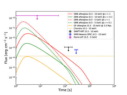
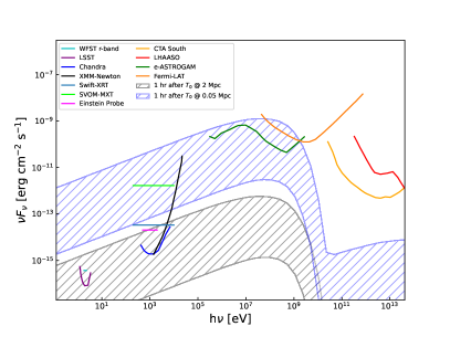
Figure 6: Light curves (left panel) and spectral energy distributions (right panel) of forward shock model. The microphysical parameters we used are $\epsilon_{e}=0.01$, $\epsilon_{b}=0.001$, $f_{e}=0.05$ and $p=2.2$. The exposure time $T_{\rm exp}$ for all the sensitivity curves we used is 1 hour. The sensitivity curves for Fermi-LAT (orange line), e-ASTROGAM (green line), LHAASO (red line) and CTA (yellow line) South are derived from de Angelis et al. (2018), and those for Chandra (blue line) and XMM-Newton (black line) are from Lucchetta et al. (2022). The other sensitivity curves are as follows: the r-band of the Legacy Survey of Space and Time (LSST) (purple line) is from Yuan et al. (2021), the r-band of Wide Field Survey Telescope (WFST; cyan line) is from Lei et al. (2023), Swift-XRT (darkcyan line) is from Burrows et al. (2005), SVOM-MXT (lime line) is from Gotz et al. (2015), and Einstein Probe (magenta line) is from Yuan et al. (2022).

If we consider GRB 231115A is a GF with $\Gamma_{0}=70$ and $E_{\gamma,\rm iso}=1.3\times 10^{45}{\rm~{}erg}$ at 3.5 Mpc, we can give the constraint for its progenitor. Following the model proposed by Murase et al. (2016), considering the magnetar generating GRB 231115A is surrounded by a wind bubble, the isotropic outflow associated with GF interacts with the nebular generating afterglow emission. The afterglow emission is associated with the nebular density $n_{\rm nb}$, which is estimated to be (Murase et al., 2016)

$$n_{\mathrm{nb}}\simeq 2.1\times 10^{3}\mathrm{~{}cm}^{-3}M_{\mathrm{nb},-7}P_{i,-0.5}^{6/5}M_{\mathrm{ext},0.5}^{3/5}V_{\mathrm{ext},8.75}^{-9/5}T_{10\;\mathrm{yr}}^{-3},$$ (10)

where $M_{\rm nb}\sim 10^{-7}~{}M_{\odot}$ is the nebular mass (which is comparable to the ejecta mass for 2004 GF of SGR 1806-20 (Gaensler et al., 2005), $P_{i}\sim 300{\rm~{}ms}$ is the initial rotation period of the magnetar (which is the typical value for Galactic pulsars (Faucher-Giguère & Kaspi, 2006), $M_{\mathrm{ext}}\sim 3~{}M_{\odot}$ is the mass of supernova (SN) ejecta, $V_{\mathrm{ext}}\sim 5000~{}\rm km~{}s^{-1}$ is the velocity of SN ejecta, which is the typical value for super-luminous SN (Kashiyama et al., 2016). It is noted that for the younger magnetar, the density of nebula becomes larger which leads to a stronger afterglow emission. Chandra gave the 3$\sigma$ luminosity limit of $2.3\times 10^{37}{\rm~{}erg~{}s^{-1}}$ (0.3–10 keV) based on the fact that no visible signal is detected in the direction of M82 (with a total exposure time of about 561 ks) (Kong & Li, 2023), as shown in the yellow dotted line in the left panel of Figure 6. Combined with this upper limit, we find that the age of the magnetar should be larger than $574{\rm~{}yr}$ with the typical microphysical parameters including $\epsilon_{e}=0.01$, $\epsilon_{b}=0.001$, $f_{e}=0.05$, and $p=2.2$. In the left panel of Figure 6, the yellow solid line shows the afterglow emission with $T=574{\rm~{}yr}$, which is just smaller than the upper limit of Chandra.

For this type of sources, we also explore the possibility of future multi-wavelength observations, as shown in the right panel of Figure 6. First, for GFs that trigger gamma-ray monitors, considering for example the current capability of Fermi-GBM (0.71 ph/cm²/s^-1 in 50–300 keV), GFs with $E_{\gamma,\rm iso}>10^{45}$ erg can be detected approximately within 10 Mpc. As shown in the blue (grey) shade in right panel of Fig 6, we modeling the spectral energy distribution starting 1 hour after trigger (and 1 hour exposure time) in the parameter space $E_{\gamma,\rm iso}$ from 10⁴⁵ to 10⁴⁷ erg, $\Gamma_{0}$ from 10 to 90, $\epsilon_{e}=0.01$, $\epsilon_{b}=0.001$, $f_{e}=0.05$, $n_{e}=0.01{\rm~{}cm^{-3}}$, $p=2.2$ and $d_{L}$ = 0.05(2) Mpc. The sensitivity of the relevant facilities is converted to an exposure time of 1 hour by assuming $F_{\rm limit}\propto T_{\rm exp}^{-0.5}$. According to the modeling results and the discussion in Fan et al. (2005), we are also expected to observe possible high-energy afterglow for such events in our local galaxy.

5 Summary and Discussion

In this work, we conducted a detailed analysis of GRB 231115A, which may have originated from a magnetar giant flare, and its features can be summarized as follows:

• There is a high probability (coincidence probability $\sim$ 0.03%) that the host galaxy is M82 with a luminosity distance of 3.5 Mpc.

• The duration is very short and there is no significant quasi-periodic signal.

• Both the time-integrated spectrum and the time-resolved spectrum can be described by an approximate quasi-thermal model (mBB). Considering the photospheric emission at different luminosity distance (3.5 Mpc, $z=0.1$, $z=1$), the roughly derived initial Lorentz factors are $\Gamma_{1}=70$, $\Gamma_{2}=240$, and $\Gamma_{3}=640$.

• The characteristics of prompt emission, such as hardness ratio and spectral lag, are consistent with short GRBs. When considering the host galaxy M82, the $E_{{\rm p},z}$–$E_{\gamma,\rm iso}$ and $EH$ relations is consistent with that of known GFs. When the redshift $z>0.1$, the correlation relations is consistent with short GRBs.

The above features are basically consistent with GRB 200415A, including the same luminosity distance, but the energy released is an order of magnitude smaller. Furthermore, a slight difference is that the light curves of GRB 231115A rises relatively slowly, or it is a relatively flat precursor, as shown in the top panel in Figure 2. Similar GF (i.e. 960618) occurred in SGR 1627–41 (Mazets et al., 1999a; Woods et al., 1999), which also shows a relatively slowly rising. These two events (GRBs 960618, 231115A) may be another subspecies of GFs and deserve further investigation.

Based on the possible afterglow emission modeling results and the upper limit of relevant observations, we cannot simply rule out the possibility that it has a merger origin. We note that Burns (2023) made a rough estimate as a giant flare from M82 vs neutron star merger GRB with a chance alignment to be approximately 180,000 to 1 (Burns et al., 2021). Therefore, the afterglow emission of GF was also modeling under appropriate assumptions, and the age of progenitor (i.e. magnetar) was constraint to be older than 574 yr. In fact, the existing modeling results are variable because we fixed the parameters including $\epsilon_{e}$, $\epsilon_{b}$, $f_{e}$ and $n_{e}$. For solving the issue of parameter degeneracy, more accurate parameter estimation requires continuous observations in multiple bands. With more early observations, it is even possible to detect the contribution of the reverse shock (Li et al., 2022).

Currently, the computation of the simplified model is fast, and for future GF events that trigger $\gamma$-ray monitors (e.g., Fermi-GBM, SVOM-GRM), we can roughly estimate the potential for follow-up observations from related facilities (e.g., WFST, EP). Also, rapid follow-up observations are expected to measure the redshift by identifying emission lines in spectra of exact optical transient sources. This is expected to advance research on their localization and revealing their progenitors, like the property of the magnetar (Wei et al., 2023). The magnetar can be associated with different types of bursts, including GFs and the fast radio bursts (FRBs) (e.g., Kaspi & Beloborodov, 2017, for a review). Two types of models for the origin of fast radio bursts associated with magnetars have been debated (e.g., Zhang, 2023, for a review), and the multi-wavelength observations for GFs can also reveal the possible origin of FRBs.

References

- Abdollahi et al. (2020) Abdollahi, S., Acero, F., Ackermann, M., et al. 2020, ApJS, 247, 33, doi: 10.3847/1538-4365/ab6bcb
- Ajello et al. (2021) Ajello, M., Atwood, W. B., Axelsson, M., et al. 2021, ApJS, 256, 12, doi: 10.3847/1538-4365/ac0ceb
- Amati et al. (2002) Amati, L., Frontera, F., Tavani, M., et al. 2002, A&A, 390, 81, doi: 10.1051/0004-6361:20020722
- Aptekar et al. (2001) Aptekar, R. L., Frederiks, D. D., Golenetskii, S. V., et al. 2001, ApJS, 137, 227, doi: 10.1086/322530
- Ashton et al. (2019) Ashton, G., Hübner, M., Lasky, P. D., et al. 2019, ApJS, 241, 27, doi: 10.3847/1538-4365/ab06fc
- Band (1997) Band, D. L. 1997, ApJ, 486, 928, doi: 10.1086/304566
- Barat et al. (1983) Barat, C., Hayles, R. I., Hurley, K., et al. 1983, A&A, 126, 400
- Beloborodov et al. (1998) Beloborodov, A. M., Stern, B. E., & Svensson, R. 1998, ApJ, 508, L25, doi: 10.1086/311710
- Berger (2014) Berger, E. 2014, ARA&A, 52, 43, doi: 10.1146/annurev-astro-081913-035926
- Bloom et al. (2001) Bloom, J. S., Frail, D. A., & Sari, R. 2001, AJ, 121, 2879, doi: 10.1086/321093
- Buchner et al. (2014) Buchner, J., Georgakakis, A., Nandra, K., et al. 2014, A&A, 564, A125, doi: 10.1051/0004-6361/201322971
- Burns (2023) Burns, E. 2023, GRB Coordinates Network, 35038, 1
- Burns et al. (2021) Burns, E., Svinkin, D., Hurley, K., et al. 2021, ApJ, 907, L28, doi: 10.3847/2041-8213/abd8c8
- Burrows et al. (2005) Burrows, D. N., Hill, J. E., Nousek, J. A., et al. 2005, Space Sci. Rev., 120, 165, doi: 10.1007/s11214-005-5097-2
- Covino et al. (2019) Covino, S., Sandrinelli, A., & Treves, A. 2019, MNRAS, 482, 1270, doi: 10.1093/mnras/sty2720
- Curtin & Chime/Frb Collaboration (2023) Curtin, A. P., & Chime/Frb Collaboration. 2023, GRB Coordinates Network, 35070, 1
- Dalessi et al. (2023) Dalessi, S., Roberts, O. J., Veres, P., Meegan, C., & Fermi Gamma-ray Burst Monitor Team. 2023, GRB Coordinates Network, 35044, 1
- de Angelis et al. (2018) de Angelis, A., Tatischeff, V., Grenier, I. A., et al. 2018, Journal of High Energy Astrophysics, 19, 1, doi: 10.1016/j.jheap.2018.07.001
- Dichiara et al. (2013) Dichiara, S., Guidorzi, C., Amati, L., & Frontera, F. 2013, MNRAS, 431, 3608, doi: 10.1093/mnras/stt445
- Dichiara et al. (2013) Dichiara, S., Guidorzi, C., Frontera, F., & Amati, L. 2013, The Astrophysical Journal, 777, 132
- Duncan (2001) Duncan, R. C. 2001, in American Institute of Physics Conference Series, Vol. 586, 20th Texas Symposium on relativistic astrophysics, ed. J. C. Wheeler & H. Martel, 495–500, doi: 10.1063/1.1419599
- Eichler et al. (1996) Eichler, D., Livio, M., Piran, T., & Schramm, D. N. 1996, in The Big Bang and Other Explosions in Nuclear and Particle Astrophysics. Edited by SCHRAMM DAVID N. Published by World Scientific Publishing Co. Pte. Ltd, 682–684, doi: 10.1142/9789812831538_0076
- Fan et al. (2005) Fan, Y. Z., Zhang, B., & Wei, D. M. 2005, MNRAS, 361, 965, doi: 10.1111/j.1365-2966.2005.09221.x
- Faucher-Giguère & Kaspi (2006) Faucher-Giguère, C.-A., & Kaspi, V. M. 2006, ApJ, 643, 332, doi: 10.1086/501516
- Fermi GBM Team (2023) Fermi GBM Team. 2023, GRB Coordinates Network, 35035, 1
- Fong & Berger (2013) Fong, W., & Berger, E. 2013, ApJ, 776, 18, doi: 10.1088/0004-637X/776/1/18
- Fong et al. (2010) Fong, W., Berger, E., & Fox, D. B. 2010, ApJ, 708, 9, doi: 10.1088/0004-637X/708/1/9
- Foreman-Mackey et al. (2013) Foreman-Mackey, D., Hogg, D. W., Lang, D., & Goodman, J. 2013, PASP, 125, 306, doi: 10.1086/670067
- Frederiks et al. (2023) Frederiks, D., Svinkin, D., Lysenko, A., et al. 2023, GRB Coordinates Network, 35062, 1
- Frederiks et al. (2007a) Frederiks, D. D., Golenetskii, S. V., Palshin, V. D., et al. 2007a, Astronomy Letters, 33, 1, doi: 10.1134/S106377370701001X
- Frederiks et al. (2007b) Frederiks, D. D., Palshin, V. D., Aptekar, R. L., et al. 2007b, Astronomy Letters, 33, 19, doi: 10.1134/S1063773707010021
- Fruchter et al. (2006) Fruchter, A. S., Levan, A. J., Strolger, L., et al. 2006, Nature, 441, 463, doi: 10.1038/nature04787
- Gaensler et al. (2005) Gaensler, B. M., Kouveliotou, C., Gelfand, J. D., et al. 2005, Nature, 434, 1104, doi: 10.1038/nature03498
- Gehrels et al. (2005) Gehrels, N., Sarazin, C. L., O’Brien, P. T., et al. 2005, Nature, 437, 851, doi: 10.1038/nature04142
- Gehrels et al. (2006) Gehrels, N., Norris, J. P., Barthelmy, S. D., et al. 2006, Nature, 444, 1044, doi: 10.1038/nature05376
- Goldstein et al. (2021) Goldstein, A., Cleveland, W. H., & Kocevski, D. 2021, Fermi GBM Data Tools: v1.1.0. https://fermi.gsfc.nasa.gov/ssc/data/analysis/gbm
- Goldstein et al. (2017) Goldstein, A., Veres, P., Burns, E., et al. 2017, ApJ, 848, L14, doi: 10.3847/2041-8213/aa8f41
- Gotz et al. (2015) Gotz, D., Adami, C., Basa, S., et al. 2015, arXiv e-prints, arXiv:1507.00204, doi: 10.48550/arXiv.1507.00204
- Guidorzi et al. (2016) Guidorzi, C., Dichiara, S., & Amati, L. 2016, A&A, 589, A98, doi: 10.1051/0004-6361/201527642
- Guidorzi et al. (2012) Guidorzi, C., Margutti, R., Amati, L., et al. 2012, MNRAS, 422, 1785, doi: 10.1111/j.1365-2966.2012.20758.x
- Horváth et al. (2006) Horváth, I., Balázs, L. G., Bagoly, Z., Ryde, F., & Mészáros, A. 2006, A&A, 447, 23, doi: 10.1051/0004-6361:20041129
- Hou et al. (2018) Hou, S.-J., Zhang, B.-B., Meng, Y.-Z., et al. 2018, ApJ, 866, 13, doi: 10.3847/1538-4357/aadc07
- Hu et al. (2023) Hu, L., Busman, M., Gruen, D., et al. 2023, GRB Coordinates Network, 35092, 1
- Hurley et al. (1999) Hurley, K., Cline, T., Mazets, E., et al. 1999, Nature, 397, 41, doi: 10.1038/16199
- Hurley et al. (2005) Hurley, K., Boggs, S. E., Smith, D. M., et al. 2005, Nature, 434, 1098, doi: 10.1038/nature03519
- IceCube Collaboration (2023) IceCube Collaboration. 2023, GRB Coordinates Network, 35053, 1
- Israel et al. (2005) Israel, G. L., Belloni, T., Stella, L., et al. 2005, ApJ, 628, L53, doi: 10.1086/432615
- Kashiyama et al. (2016) Kashiyama, K., Murase, K., Bartos, I., Kiuchi, K., & Margutti, R. 2016, ApJ, 818, 94, doi: 10.3847/0004-637X/818/1/94
- Kaspi & Beloborodov (2017) Kaspi, V. M., & Beloborodov, A. M. 2017, ARA&A, 55, 261, doi: 10.1146/annurev-astro-081915-023329
- Kong & Li (2023) Kong, A. K. H., & Li, K. L. 2023, GRB Coordinates Network, 35054, 1
- Koshut et al. (1996) Koshut, T. M., Paciesas, W. S., Kouveliotou, C., et al. 1996, ApJ, 463, 570, doi: 10.1086/177272
- Kouveliotou et al. (1993) Kouveliotou, C., Meegan, C. A., Fishman, G. J., et al. 1993, ApJ, 413, L101, doi: 10.1086/186969
- Kumar et al. (2023) Kumar, R., Salgundi, A., Swain, V., et al. 2023, GRB Coordinates Network, 35041, 1
- Lazzati et al. (2005) Lazzati, D., Ghirlanda, G., & Ghisellini, G. 2005, MNRAS, 362, L8, doi: 10.1111/j.1745-3933.2005.00062.x
- Leahy et al. (1983) Leahy, D. A., Darbro, W., Elsner, R. F., et al. 1983, ApJ, 266, 160, doi: 10.1086/160766
- Lei et al. (2023) Lei, L., Zhu, Q.-F., Kong, X., et al. 2023, Research in Astronomy and Astrophysics, 23, 035013, doi: 10.1088/1674-4527/acb877
- Leibler & Berger (2010) Leibler, C. N., & Berger, E. 2010, ApJ, 725, 1202, doi: 10.1088/0004-637X/725/1/1202
- Li et al. (2022) Li, H.-Y., He, H.-N., Wei, D.-M., & Jin, Z.-P. 2022, MNRAS, 517, 3881, doi: 10.1093/mnras/stac2924
- Ligo Scientific Collaboration et al. (2023) Ligo Scientific Collaboration, VIRGO Collaboration, & Kagra Collaboration. 2023, GRB Coordinates Network, 35049, 1
- Lucchetta et al. (2022) Lucchetta, G., Ackermann, M., Berge, D., & Bühler, R. 2022, Journal of Cosmology and Astroparticle Physics, 2022, 013, doi: 10.1088/1475-7516/2022/08/013
- Mazets et al. (1999a) Mazets, E. P., Aptekar, R. L., Butterworth, P. S., et al. 1999a, ApJ, 519, L151, doi: 10.1086/312118
- Mazets et al. (1999b) Mazets, E. P., Cline, T. L., Aptekar’, R. L., et al. 1999b, Astronomy Letters, 25, 635, doi: 10.48550/arXiv.astro-ph/9905196
- Mazets et al. (1982) Mazets, E. P., Golenetskii, S. V., Gurian, I. A., & Ilinskii, V. N. 1982, Ap&SS, 84, 173, doi: 10.1007/BF00713635
- Mazets et al. (1979) Mazets, E. P., Golentskii, S. V., Ilinskii, V. N., Aptekar, R. L., & Guryan, I. A. 1979, Nature, 282, 587, doi: 10.1038/282587a0
- Mazets et al. (2008a) Mazets, E. P., Aptekar, R. L., Cline, T. L., et al. 2008a, ApJ, 680, 545, doi: 10.1086/587955
- Mazets et al. (2008b) —. 2008b, ApJ, 680, 545, doi: 10.1086/587955
- Meegan et al. (2009) Meegan, C., Lichti, G., Bhat, P. N., et al. 2009, ApJ, 702, 791, doi: 10.1088/0004-637X/702/1/791
- Mereghetti et al. (2023) Mereghetti, S., Gotz, D., Ferrigno, C., et al. 2023, GRB Coordinates Network, 35037, 1
- Minaev et al. (2023) Minaev, P., Pozanenko, A., & GRB IKI FuN. 2023, GRB Coordinates Network, 35059, 1
- Minaev & Pozanenko (2020a) Minaev, P. Y., & Pozanenko, A. S. 2020a, MNRAS, 492, 1919, doi: 10.1093/mnras/stz3611
- Minaev & Pozanenko (2020b) —. 2020b, Astronomy Letters, 46, 573, doi: 10.1134/S1063773720090042
- Murase et al. (2016) Murase, K., Kashiyama, K., & Mészáros, P. 2016, MNRAS, 461, 1498, doi: 10.1093/mnras/stw1328
- Narayan et al. (1992) Narayan, R., Paczynski, B., & Piran, T. 1992, ApJ, 395, L83, doi: 10.1086/186493
- Norris (2002) Norris, J. P. 2002, ApJ, 579, 386, doi: 10.1086/342747
- Norris & Bonnell (2006) Norris, J. P., & Bonnell, J. T. 2006, ApJ, 643, 266, doi: 10.1086/502796
- Norris et al. (2004) Norris, J. P., Bonnell, J. T., Kazanas, D., et al. 2004, in American Astronomical Society Meeting Abstracts, Vol. 205, American Astronomical Society Meeting Abstracts, 68.04
- Norris et al. (2000) Norris, J. P., Marani, G. F., & Bonnell, J. T. 2000, ApJ, 534, 248, doi: 10.1086/308725
- Osborne et al. (2023) Osborne, J. P., Sbarufatti, B., D’Ai, A., et al. 2023, GRB Coordinates Network, 35064, 1
- Palmer et al. (2005) Palmer, D. M., Barthelmy, S., Gehrels, N., et al. 2005, Nature, 434, 1107, doi: 10.1038/nature03525
- Pe’er et al. (2007) Pe’er, A., Ryde, F., Wijers, R. A. M. J., Mészáros, P., & Rees, M. J. 2007, ApJ, 664, L1, doi: 10.1086/520534
- Popov & Stern (2006) Popov, S. B., & Stern, B. E. 2006, MNRAS, 365, 885, doi: 10.1111/j.1365-2966.2005.09767.x
- Preece et al. (2002) Preece, R. D., Briggs, M. S., Giblin, T. W., et al. 2002, ApJ, 581, 1248, doi: 10.1086/344252
- Preece et al. (1998) Preece, R. D., Briggs, M. S., Mallozzi, R. S., et al. 1998, ApJ, 506, L23, doi: 10.1086/311644
- Ren et al. (2023) Ren, J., Wang, Y., & Dai, Z.-G. 2023, arXiv e-prints, arXiv:2310.15886, doi: 10.48550/arXiv.2310.15886
- Rigoselli et al. (2023) Rigoselli, M., Pacholski, D. P., Mereghetti, S., R. Salvaterra (INAF, I.-M., & S. Campana (INAF, O. 2023, GRB Coordinates Network, 35175, 1
- Roberts et al. (2021) Roberts, O. J., Veres, P., Baring, M., et al. 2021, in American Astronomical Society Meeting Abstracts, Vol. 53, American Astronomical Society Meeting Abstracts, 233.02
- Ryde et al. (2010) Ryde, F., Axelsson, M., Zhang, B. B., et al. 2010, ApJ, 709, L172, doi: 10.1088/2041-8205/709/2/L172
- Strohmayer & Watts (2005) Strohmayer, T. E., & Watts, A. L. 2005, ApJ, 632, L111, doi: 10.1086/497911
- Svinkin et al. (2021) Svinkin, D., Frederiks, D., Hurley, K., et al. 2021, Nature, 589, 211, doi: 10.1038/s41586-020-03076-9
- Tanaka et al. (2007) Tanaka, Y. T., Terasawa, T., Kawai, N., et al. 2007, ApJ, 665, L55, doi: 10.1086/521025
- Thrane & Talbot (2019) Thrane, E., & Talbot, C. 2019, Publications of the Astronomical Society of Australia, 36
- Ukwatta et al. (2010) Ukwatta, T. N., Stamatikos, M., Dhuga, K. S., et al. 2010, ApJ, 711, 1073, doi: 10.1088/0004-637X/711/2/1073
- van de Schoot et al. (2021) van de Schoot, R., Depaoli, S., King, R., et al. 2021, Nature Reviews Methods Primers, 1, 1
- Vaughan (2005) Vaughan, S. 2005, A&A, 431, 391, doi: 10.1051/0004-6361:20041453
- Vaughan (2010) —. 2010, MNRAS, 402, 307, doi: 10.1111/j.1365-2966.2009.15868.x
- Vaughan (2012) —. 2012, Philosophical Transactions of the Royal Society of London Series A, 371, 20110549, doi: 10.1098/rsta.2011.0549
- Wang et al. (2023) Wang, Y., Xia, Z.-Q., Zheng, T.-C., Ren, J., & Fan, Y.-Z. 2023, ApJ, 953, L8, doi: 10.3847/2041-8213/ace7d4
- Watts & Strohmayer (2006) Watts, A. L., & Strohmayer, T. E. 2006, ApJ, 637, L117, doi: 10.1086/500735
- Wei et al. (2023) Wei, Y., Zhang, B. T., & Murase, K. 2023, MNRAS, 524, 6004, doi: 10.1093/mnras/stad2122
- Woods et al. (1999) Woods, P. M., Kouveliotou, C., van Paradijs, J., et al. 1999, ApJ, 519, L139, doi: 10.1086/312124
- Woosley (1993) Woosley, S. E. 1993, ApJ, 405, 273, doi: 10.1086/172359
- Yang et al. (2020) Yang, J., Chand, V., Zhang, B.-B., et al. 2020, ApJ, 899, 106, doi: 10.3847/1538-4357/aba745
- Yi et al. (2006) Yi, T., Liang, E., Qin, Y., & Lu, R. 2006, MNRAS, 367, 1751, doi: 10.1111/j.1365-2966.2006.10083.x
- Yuan et al. (2021) Yuan, C., Murase, K., Zhang, B. T., Kimura, S. S., & Mészáros, P. 2021, ApJ, 911, L15, doi: 10.3847/2041-8213/abee2410.48550/arXiv.2101.05788
- Yuan et al. (2022) Yuan, W., Zhang, C., Chen, Y., & Ling, Z. 2022, in Handbook of X-ray and Gamma-ray Astrophysics, 86, doi: 10.1007/978-981-16-4544-0_151-1
- Zhang (2023) Zhang, B. 2023, Reviews of Modern Physics, 95, 035005, doi: 10.1103/RevModPhys.95.035005
- Zhang et al. (2020) Zhang, H.-M., Liu, R.-Y., Zhong, S.-Q., & Wang, X.-Y. 2020, ApJ, 903, L32, doi: 10.3847/2041-8213/abc2c9