A complex-projected Rayleigh quotient iteration for targeting interior eigenvalues

Abstract

We introduce a new Projected Rayleigh Quotient Iteration aimed at improving the convergence behaviour of classic Rayleigh Quotient iteration (RQI) by incorporating approximate information about the target eigenvector at each step. While classic RQI exhibits local cubic convergence for Hermitian matrices, its global behaviour can be unpredictable, whereby it may converge to an eigenvalue far away from the target, even when started with accurate initial conditions. This problem is exacerbated when the eigenvalues are closely spaced. The key idea of the new algorithm is at each step to add a complex-valued projection to the original matrix (that depends on the current eigenvector approximation), such that the unwanted eigenvalues are lifted into the complex plane while the target stays close to the real line, thereby increasing the spacing between the target eigenvalue and the rest of the spectrum. Making better use of the eigenvector approximation leads to more robust convergence behaviour and the new method converges reliably to the correct target eigenpair for a significantly wider range of initial vectors than does classic RQI. We prove that the method converges locally cubically and we present several numerical examples demonstrating the improved global convergence behaviour. In particular, we apply it to compute eigenvalues in a band-gap spectrum of a Sturm-Liouville operator used to model photonic crystal fibres, where the target and unwanted eigenvalues are closely spaced. The examples show that the new method converges to the desired eigenpair even when the eigenvalue spacing is very small, often succeeding when classic RQI fails.

1 Introduction

Rayleigh Quotient Iteration (RQI) is a simple yet effective algorithm to compute a single eigenvalue and eigenvector pair (eigenpair) of a matrix. For Hermitian matrices, RQI converges locally cubically and converges globally for almost all starting vectors [21], but it suffers from a significant flaw, whereby the global convergence can be unpredictable. It is well-known that RQI may converge to the wrong eigenpair, i.e., one that is different to the target eigenpair, even when executed with a good approximation of the target eigenvector as the initial vector and an initial shift close to the target eigenvalue. This problem is exacerbated in cases where the distance between the wanted eigenvalue and its neighbours is small (cf. the numerical examples in Section 4).

In this paper, we propose a new algorithm that modifies RQI to overcome this problem by exploiting any prior information known about the target eigenvector. The idea of the new method is as follows. Starting with an approximation of the target eigenvector, we perturb the original problem by adding a purely complex projection matrix constructed using this approximation, such that the unwanted eigenvalues are lifted into the complex plane, while the target eigenvalue remains close to the real line (see Figure 1 in Section 3), thereby artificially increasing the gap between the target eigenvalue and its neighbours. We then use the perturbed matrix in RQI, where in each step of the iteration we update the perturbation matrix using the previous eigenvector approximation and gradually reduce the size of the perturbation.

More precisely, suppose we wish to compute an eigenpair $(\lambda,\bm{v})\in\mathbb{R}\times\mathbb{C}^{n}$, $\bm{v}\neq\bm{0}$, of a Hermitian matrix $A\in\mathbb{C}^{n\times n}$ and we are given an approximation $\bm{u}\approx\bm{v}$, then we perturb the matrix $A$ by

$$A\longrightarrow A+i\gamma(I-\bm{u}\bm{u}^{\ast})\,,$$

where $i$ denotes the imaginary unit, the asterisk denotes the complex conjugate transpose and $I-\bm{u}\bm{u}^{*}$ is the projection onto the orthogonal complement of $\bm{u}$. The real scalar $\gamma>0$ is used to control the magnitude of the perturbation.

If $\bm{u}$ is a sufficiently good approximation of $\bm{v}$, then the perturbed target eigenvalue $\widetilde{\lambda}$ stays near the real line while the remaining eigenvalues, $\mu\neq\lambda$, are perturbed by

$$\mu\longrightarrow\mu+i\gamma\,,$$

approximately. Since $\mu\in\mathbb{R}$, because $A$ is Hermitian, the perturbed eigenvalues now lie (approximately) along the line $i\gamma$ in the upper half of the complex plane, again see Figure 1, and so the distance between the perturbed target eigenvalue $\widetilde{\lambda}$ and the remainder of the perturbed spectrum is approximately $\gamma$. Applying RQI to this problem, we will not compute the target eigenvalue but rather an eigenvalue of the perturbed matrix. Therefore, we replace $\gamma$ by a non-negative decreasing zero sequence ${(\gamma^{(k)})}_{k\geq 0}\subset\mathbb{R}$ such that the perturbation becomes increasingly small as $k\rightarrow\infty$ and we recover the original unperturbed problem. If the sequence ${(\gamma^{(k)})}_{k\geq 0}$ is chosen to decay sufficiently fast, then asymptotically our algorithm converges like classic RQI either cubically or quadratically to an eigenpair.

The motivation comes from practical applications where the eigenvalues are closely spaced but some information about the target eigenvector is known. For example, in models for photonic crystal fibres [16] the spectrum has a band-gap structure and the eigenvalues that lie inside the gaps are very closely spaced; the corresponding eigenvectors are oscillatory and localised. As we show later in Section 4, this limited, qualitative information about the target eigenvector suffices to ensure that our method converges to it. The method we propose was inspired by the approach in [18], which works directly on the differential equation level. See also the recent article [19], which expands on that paper. Alternative numerical methods for computing localised eigenfunctions of differential operators are presented in [4, 5, 3]. In contrast to all those methods, our approach is purely algebraic, can be applied to any Hermitian matrix and requires only a one-line change in a classic RQI algorithm.

There are other approaches that modify RQI in order to make the convergence behaviour of the algorithm more predictable, see [20, 24, 7]. However, all those methods usually use a priori information about the eigenvalues, e.g., the number of eigenvalues within a certain interval. Our approach is novel in that we exploit information about the eigenvectors instead.

The remainder of the paper is organised as follows. In the next section, we review convergence results for Inverse Iteration and classic RQI, since they form the basis for the convergence analysis of our method. In Section 3, we then introduce the new Projected Rayleigh Quotient Iteration (PRQI) method. We also prove there that the approach introduced above is equivalent to perturbing the matrix according to

$$A\longrightarrow A+i\gamma I\,.$$

That is, it is not necessary to perturb $A$ by the full projection matrix $i\gamma(I-\bm{u}\bm{u}^{\ast})$ but it suffices to shift only the diagonal entries by $i\gamma$. This simplifies the implementation and also allows to prove asymptotic convergence for our method. Finally, in Section 4 we present three numerical examples that demonstrate the efficacy of our method, including a practical example from an application in photonics. In particular, we present results where our algorithm succeeds in locating the target eigenvalue within a closely-spaced spectrum. Often a crude approximation is sufficient for our method to succeed in converging to the target eigenpair, while for the same initial conditions classic RQI fails.

2 Classic Rayleigh Quotient Iteration

We consider the Hermitian eigenvalue problem: find $(\lambda,\bm{v})\in\mathbb{R}\times\mathbb{C}^{n}$, $\bm{v}\neq\bm{0}$, such that

$$A\bm{v}=\lambda\bm{v}\,,$$ (2.1)

where $A=A^{\ast}\in\mathbb{C}^{n\times n}$ is a complex Hermitian matrix. We denote the eigenvalues of $A$ by $\lambda_{1},\dotsc,\lambda_{n}$ with corresponding eigenvectors $\bm{v}_{1},\dotsc,\bm{v}_{n}$ which we assume to be normalised w.r.t. the Euclidean norm $\left\lVert\cdot\right\rVert=\left\lVert\cdot\right\rVert_{2}$. For simplicity, we assume the target eigenvalue is simple, i.e., it has algebraic multiplicity 1. The eigenvalues will usually be labelled such that $\lambda_{1}$ is the target eigenvalue (see, e.g., Theorem 2.1 below).

There are a wide variety of methods that can be used to solve (2.1) numerically, see, e.g., the monographs [23] and [9]. One of the most widely used and simplest methods is the (shifted) inverse iteration. Starting with a non-zero vector $\bm{x}^{(0)}$ and a shift $\mu\in\mathbb{R}$, one computes

$$\bm{x}^{(k+1)}=\alpha^{(k)}{(A-\mu I)}^{-1}\bm{x}^{(k)}\,,\quad k=0,1,\dotsc$$ (2.2)

where $I$ denotes the $n\times n$ identity matrix and $\alpha^{(k)}$ is a scalar responsible for normalising $\bm{x}^{(k+1)}$. The sequence ${(\bm{x}^{(k)})}_{k}$ converges linearly to the eigenvector that corresponds to the eigenvalue closest to the shift $\mu$. More precisely, we have the following convergence result. Here, $\theta(\bm{u},\bm{w})$ denotes the angle between the vectors $\bm{u}$ and $\bm{w}$, i.e.,

$$\theta(\bm{u},\bm{w})=\arccos\bigg{(}\frac{\left\lvert\bm{u}^{\ast}\bm{w}\right\rvert}{\left\lVert\bm{u}\right\rVert\left\lVert\bm{w}\right\rVert}\bigg{)}\,.$$ (2.3)

Theorem 2.1 ([9], Theorem 4.10).

Let $\mu\in\mathbb{R}$ be such that $A-\mu I$ is invertible, i.e., $\mu$ is not an eigenvalue of $A$, and label the eigenvalues of $A$ such that

$$\left\lvert\lambda_{1}-\mu\right\rvert<\left\lvert\lambda_{2}-\mu\right\rvert\leq\cdots\leq\left\lvert\lambda_{n}-\mu\right\rvert\,.$$

Then, for the sequence ${(\bm{x}^{(k)})}_{k\geq 0}$ generated by Inverse Iteration (2.2), we have

$$\tan\big{(}\theta(\bm{x}^{(k+1)},\bm{v}_{1})\big{)}\leq\frac{\left\lvert\lambda_{1}-\mu\right\rvert}{\left\lvert\lambda_{2}-\mu\right\rvert}\tan\big{(}\theta(\bm{x}^{(k)},\bm{v}_{1})\big{)}\,.$$

Inverse Iteration as given in (2.2) only yields approximations of an eigenvector. To obtain an approximation of the corresponding eigenvalue the Rayleigh Quotient can be used.

Definition 2.2 (Rayleigh Quotient).

Let $A\in\mathbb{C}^{n\times n}$. The mapping

$$\mathcal{R}_{A}:\mathbb{C}^{n}\setminus\{\bm{0}\}\rightarrow\mathbb{C},\qquad\bm{x}\mapsto\frac{\bm{x}^{\ast}A\bm{x}}{\bm{x}^{\ast}\bm{x}}$$

is called the Rayleigh Quotient corresponding to the matrix $A$.

The following result specifies the quality of the Rayleigh Quotient as an estimate for the eigenvalue.

Theorem 2.3 ([9], Theorem 4.6).

Let $A\in\mathbb{C}^{n\times n}$ be Hermitian, let $\bm{x}\in\mathbb{C}^{n}$ be a nonzero vector and let $(\lambda,\bm{v})$ be an eigenpair of $A$. Then

$$\left\lvert\mathcal{R}_{A}(\bm{x})-\lambda\right\rvert\leq\left\lVert A-\lambda I\right\rVert\tan^{2}\big{(}\theta(\bm{x},\bm{v})\big{)}\,,$$ (2.4)

that is, the Rayleigh Quotient is a quadratically accurate estimate of an eigenvalue.

It is now quite natural to replace the fixed shift $\mu$ in inverse iteration by the Rayleigh Quotient of the current vector iterate. The resulting algorithm is called Rayleigh Quotient Iteration (RQI) and is summarised in Algorithm 2.1.

Algorithm 2.1 Classic Rayleigh Quotient Iteration

1:$\bm{x}\in\mathbb{C}^{n}$ with $\|\bm{x}^{(0)}\|=1$

2:for $k=0,1,2,\dotsc$, until convergence do

3:     $\mu^{(k)}\leftarrow{(\bm{x}^{(k)})}^{\ast}A\bm{x}^{(k)}$ $\triangleright$ Compute the Rayleigh Quotient

4:     Solve $(A-\mu^{(k)}I)\bm{y}^{(k+1)}=\bm{x}^{(k)}$ for $\bm{y}^{(k+1)}$

5:     $\bm{x}^{(k+1)}\leftarrow\bm{y}^{(k+1)}/\|{\bm{y}^{(k+1)}}\|$ $\triangleright$ Normalise

6:end for

Note that in the computation of the Rayleigh Quotient in Step 2, dividing by ${(\bm{x}^{(k)})}^{\ast}\bm{x}^{(k)}$ has been omitted, because the vector iterates are always normalised.

In practice, the iteration is stopped when the the approximation is deemed to have converged to within a given tolerance $\textsc{tol}>0$ or a maximum number of iterations is reached. The most common test for convergence is when the norm of the residual,

$$\bm{r}^{(k)}\coloneqq(A-\mu^{(k)}I)\bm{x}^{(k)},$$ (2.5)

is below the tolerance tol or the scaled tolerance $\mu^{(k)}\times\textsc{tol}$. The use of the residual as a convergence test is justified by the following a posteriori bounds on the errors.

Proposition 2.4 ([23], Cor. 3.4 and Thm. 3.9).

Let $\bm{u}\in\mathbb{C}^{n}$ with $\left\lVert\bm{u}\right\rVert=1$ and let $\mu=\mathcal{R}_{A}(\bm{u})$ be the corresponding Rayleigh quotient. Let $(\lambda,\bm{v})$ be an eigenpair of $A$ such that $\lambda$ is the eigenvalue closest to $\mu$ and let $\delta>0$ be the distance from $\lambda$ to the rest of the spectrum. Then the residual, $\bm{r}=(A-\mu I)\bm{u}$, satisfies

$$|\mu-\lambda|\leq\frac{\left\lVert\bm{r}\right\rVert^{2}}{\delta}\qquad\text{and}\qquad\sin\theta(\bm{u},\bm{v})\leq\frac{\left\lVert\bm{r}\right\rVert}{\delta}\,.$$

Although these bounds depend inversely on the eigenvalue gap, and therefore become inaccurate if the target eigenvalue $\lambda$ is not well-separated from its neighbours, a residual based stopping criterion is often the only option to determine convergence. Since RQI converges locally cubically (see below), it is usually sufficient to perform one additional iteration after the stopping criterion is satisfied to guarantee that the computed eigenvalue and eigenvector approximation are sufficiently accurate.

Theorem 2.5 ([9], Proposition 4.13).

For an initial vector $\bm{x}^{(0)}\in\mathbb{C}^{n}$, let ${(\bm{x}^{(k)})}_{k\geq 0}$ be the sequence of vectors generated by RQI and let $\mu^{(k)}=\mathcal{R}_{A}(\bm{x}^{(k)})$ for $k\geq 0$. Assume that $A-\mu^{(0)}I$ is invertible and label the eigenvalues of $A$ such that

$$\big{|}{\lambda_{1}-\mu^{(0)}}\big{|}<\big{|}{\lambda_{2}-\mu^{(0)}}\big{|}\leq\cdots\leq\big{|}{\lambda_{n}-\mu^{(0)}}\big{|}\,.$$ (2.6)

Suppose that there exists a constant $c>0$ such that

$$\tan\big{(}\theta(\bm{x}^{(0)},\bm{v}_{1})\big{)}\leq c\leq\sqrt{\frac{\left\lvert\lambda_{1}-\lambda_{2}\right\rvert}{2\left\lVert A-\lambda_{1}I\right\rVert}}\,,$$ (2.7)

then the next RQI iterate $\bm{x}^{(1)}$ satisfies

$$\tan\big{(}\theta(\bm{x}^{(1)},\bm{v}_{1})\big{)}\leq 2\frac{\left\lVert A-\lambda_{1}I\right\rVert}{\left\lvert\lambda_{1}-\lambda_{2}\right\rvert}\tan^{3}\big{(}\theta(\bm{x}^{(0)},\bm{v}_{1})\big{)}\leq c\,,$$

i.e., RQI is locally cubically convergent.

Although the condition in (2.7) is only sufficient but not necessary to ensure convergence to the target eigenvector, it suggests that very accurate initial vectors $\bm{x}^{(0)}$ are required to ensure convergence to the target eigenpair when the gap $\left\lvert\lambda_{1}-\lambda_{2}\right\rvert$ is small. When the initial vector is not well-aligned with the target eigenspace, the convergence behaviour of RQI is difficult to predict. In [6], the dependence of the basins of attraction around the eigenvectors on the eigenvalue gap is studied. For the $3\times 3$ case it is shown that the basins deteriorate when the eigenvalues around the target eigenvalue are closely spaced; analogous observations and visualisations can also be found in [20, 1]. In Section 4, we provide similar visualisations for RQI and our method, which demonstrate a significantly reduced dependence on the eigenvalue gap of our method.

The idea of modifying RQI to make it more predictable is not new. However, most approaches are aimed at designing methods that ensure convergence to an eigenvalue near the initial shift or in a predefined interval [24, 7]. These approaches are not suitable, however, for very closely spaced eigenvalues. Our goal is to modify RQI so that it utilises the information in the initial vector $\bm{x}^{(0)}$ rather than the initial shift. In this way, the convergence becomes more predictable and less dependent on the eigenvalue gap.

3 Projected Rayleigh Quotient Iteration

In this section, we present the new Projected Raleigh Quotient Iteration (PRQI), along with a simplified version of the algorithm and an analysis of the local convergence properties. First, we provide some intuition behind the main idea of introducing a complex projection into the shift.

Suppose that $\bm{u}\in\mathbb{C}^{n}$ is a unit norm approximation for one of the eigenvectors of a Hermitian matrix $A\in\mathbb{C}^{n\times n}$. After relabelling we may assume that $\bm{u}$ approximates $\bm{v}_{1}$, which we shall refer to as the target eigenvector. Expanding $\bm{u}$ in the eigenbasis of $A$, we can write

$$\bm{u}=\sum_{j=1}^{n}\alpha_{j}\bm{v}_{j}\,,$$

where $\left\lvert\alpha_{1}\right\rvert\approx 1$ and $\left\lvert\alpha_{j}\right\rvert\ll 1$ for $j>1$, because $\bm{u}\approx\bm{v}_{1}$. Now, consider the projection onto the orthogonal complement of the span of $\bm{u}$, given by the matrix $I-\bm{u}\bm{u}^{\ast}$. Adding this projection to $A$, with a complex scaling, for some eigenvector $\bm{v}_{m}$ we have

$$\big{[}A+i(I-\bm{u}\bm{u}^{\ast})\big{]}\bm{v}_{m} =\bigg{[}A+i\bigg{(}I-\sum_{j,k=1}^{n}\alpha_{j}\alpha_{k}^{\ast}\bm{v}_{j}\bm{v}_{k}^{\ast}\bigg{)}\bigg{]}\bm{v}_{m}$$

$$=\lambda_{m}\bm{v}_{m}+i\bigg{(}\bm{v}_{m}-\alpha_{m}^{\ast}\sum_{j=2}^{n}\alpha_{j}\bm{v}_{j}-\alpha_{m}^{\ast}\alpha_{1}\bm{v}_{1}\bigg{)}\,.$$

If $\lambda_{m}$ is not the target eigenvalue, i.e., $m\neq 1$, then the last two terms inside the bracket are approximately zero and we have

$$\big{[}A+i(I-\bm{u}\bm{u}^{\ast})\big{]}\bm{v}_{m}\approx(\lambda_{m}+i)\bm{v}_{m},\quad\text{for }m>1\,.$$

On the other hand, for $m=1$, since $|\alpha_{j}|\ll 1$ for $j>1$, the sum is approximately zero and since $|\alpha_{1}|\approx 1$ we have

$$\big{[}A+i(I-\bm{u}\bm{u}^{\ast})\big{]}\bm{v}_{1}\approx\lambda_{1}\bm{v}_{1}+i\bm{v}_{1}-i\left\lvert\alpha_{1}\right\rvert^{2}\bm{v}_{1}\approx\lambda_{1}\bm{v}_{1}\,.$$

Hence, perturbing the matrix $A$ by $i(I-\bm{u}\bm{u}^{\ast})$ we expect that the eigenvalue corresponding to $\bm{v}_{1}$ to be barely affected while the remaining eigenvalues will be shifted by approximately $i$.

To control the magnitude of the perturbation, we introduce the (real) scalar $\gamma>0$ and consider instead

$$A\longrightarrow A+i\gamma(I-\bm{u}\bm{u}^{\ast})=:\widetilde{A}\,.$$ (3.1)

Denoting the eigenvalues of the perturbed matrix $\widetilde{A}$ by $\widetilde{\lambda}_{m}$, following the arguments above we have

$$\widetilde{\lambda}_{1}\approx\lambda_{1}\qquad\text{and}\qquad\widetilde{\lambda}_{m}\approx\lambda_{m}+i\gamma\quad\text{for }m>1\,,$$ (3.2)

i.e., the eigenvalues of $A$ (except for the target eigenvalue $\lambda_{1}$) are raised into the complex plane and the distance between the target eigenvalue and the remaining eigenvalues is now approximately $\gamma$, see Figure 1.

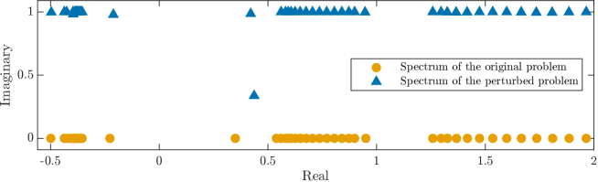
Figure 1: Section of the spectrum of a matrix $A$ (orange circles) and the perturbed matrix $\widetilde{A}$ (blue triangles) for $\gamma=1$. Most of the perturbed eigenvalues $\widetilde{\lambda}$ have $\text{Im}({\widetilde{\lambda}})\approx 1$ while one eigenvalue lies close to the real line. The matrix $A$ and the vector $\bm{u}$ that were used to construct $\widetilde{A}$ for this plot come from Example 3 in Section 4.

As remarked in the introduction, the basins of attractions of RQI depend critically on the eigenvalue gap. By increasing the eigenvalue gap we expect the basin of attraction around the target eigenvector to increase, thus making the algorithm more likely to succeed.

Of course, by applying RQI to the matrix $\widetilde{A}$ defined in (3.1), we would compute an eigenpair of $\widetilde{A}$ instead of $A$. Therefore, we replace the fixed shift $\gamma$ by a non-negative sequence ${(\gamma^{(k)})}_{k\geq 0}$ that converges to 0 and we replace the initial approximation $\bm{u}$ by the current vector iterate $\bm{x}^{(k)}$. The full iteration is summarised in Algorithm 3.1. The stopping criteria can be chosen to be the same as for classic RQI, e.g., terminating when either the norm of the residual (2.5) is below a given tolerance or a maximum number of iterations is reached.

For real symmetric problems, the eigenvectors are real but due to the imaginary shift, the final vector iterate $\bm{x}^{(K)}$ typically still contains a non-zero imaginary part. We therefore usually perform one step of classic RQI applied to $\operatorname{Re}(\bm{x}^{(K)})$ after the loop ($\operatorname{Re}(\cdot)$ denotes the component-wise real part).

Algorithm 3.1 Projected Rayleigh Quotient Iteration (full version)

1:$\bm{x}^{(0)}\in\mathbb{C}^{n}$ with $\|\bm{x}^{(0)}\|=1$

2:for $k=0,1,2,\dotsc$, until stopping criteria are satisfied do

3:     $\mu^{(k)}\leftarrow{(\bm{x}^{(k)})}^{\ast}A\bm{x}^{(k)}$ $\triangleright$ Compute the Rayleigh Quotient

4:     Update $\gamma^{(k)}$ $\triangleright$ Update scaling factor

5:     Solve $\big{[}A-\mu^{(k)}I+i\gamma^{(k)}(I-\bm{x}^{(k)}{(\bm{x}^{(k)})}^{\ast})\big{]}\bm{y}^{(k+1)}=\bm{x}^{(k)}$ for $\bm{y}^{(k+1)}$

6:     $\bm{x}^{(k+1)}\leftarrow\bm{y}^{(k+1)}/\|\bm{y}^{(k+1)}\|$ $\triangleright$ Normalise

7:end for

Note that in practice we allow each $\gamma^{(k)}$ to depend on the previous iterates $\bm{x}^{(0)},$ $\bm{x}^{(1)},\ldots,\,\bm{x}^{(k)}$. Hence, the sequence ${(\gamma^{(k)})}_{k\geq 0}$ is not an input to Algorithm 3.1, but instead we have included Step 3 where $\gamma^{(k)}$ is updated. How the sequence ${(\gamma^{(k)})}_{k\geq 0}$ should be chosen to ensure both stability of the iteration and rapid convergence, is discussed in Section 3.2. First, we derive a simplified version of the algorithm.

3.1 A simplified algorithm

The solution of the linear system in Step 4 of Algorithm 3.1 requires the solution of the rank-one updated system

$$\big{[}\widetilde{A}^{(k)}-i\gamma^{(k)}\bm{x}^{(k)}{(\bm{x}^{(k)})}^{\ast}\big{]}\bm{y}^{(k+1)}=\bm{x}^{(k)}\,,$$

where

$$\widetilde{A}^{(k)}\coloneqq A-\mu^{(k)}I+i\gamma^{(k)}I\,.$$

Such systems can be solved by first solving $\widetilde{A}^{(k)}\bm{z}^{(k)}=\bm{x}^{(k)}$ and then updating the solution using the Sherman–Morrison formula as described in, e.g., [14]. We now show that updating the solution is not necessary because solving $\widetilde{A}^{(k)}\bm{z}^{(k)}=\bm{x}^{(k)}$ and normalising the solution produces the same iterates as Algorithm 3.1.

Lemma 3.1.

Let $A\in\mathbb{C}^{n\times n}$ be Hermitian and $\bm{u}\in\mathbb{C}^{n}$ with $\|\bm{u}\|=1$. Define the matrices

$$B\coloneqq A-\mu I+i\gamma I\quad\text{and}\quad C\coloneqq{A-\mu I+i\gamma(I-\bm{u}\bm{u}^{\ast})}\,,$$

where $\gamma>0$ and $\mu\in\mathbb{R}$ is such that $(\bm{u},\mu)$ is not an eigenpair of $A$. Then, both $B$ and $C$ are invertible and $B^{-1}\bm{u}$ is a scalar multiple of $C^{-1}\bm{u}$.

Proof.

Writing $B=A-(\mu-i\gamma)I$, we see that $B$ is singular if and only if $\mu-i\gamma$ is an eigenvalue of $A$. Since $A$ is Hermitian all of its eigenvalues are real, but since $\gamma>0$, we have $\mu-i\gamma\in\mathbb{C}\setminus\mathbb{R}$, which cannot be an eigenvalue of $A$. Thus, $B$ is invertible.

Now, observe that $C=B-i\gamma\bm{u}\bm{u}^{\ast}$. The Sherman–Morrison formula (see, e.g., [12, p. 50]) states that $C$ is invertible if $i\gamma\bm{u}^{\ast}B^{-1}\bm{u}\neq-1$. To check that this holds, let $A=VDV^{\ast}$ be an eigendecomposition of $A$ with a unitary matrix $V$, whose columns are the eigenvectors of $A$, and a diagonal matrix $D=\mathrm{diag}(\lambda_{1},\dotsc,\lambda_{n})$ containing the corresponding eigenvalues. We then have $B=V(D-\mu I+i\gamma I)V^{\ast}$ and consequently

$$B^{-1}={(V^{\ast})}^{-1}{(D-\mu I+i\gamma I)}^{-1}V^{-1}=V{(D-\mu I+i\gamma I)}^{-1}V^{\ast}\,.$$

Thus,

$$\bm{u}^{\ast}B^{-1}\bm{u} =\bm{u}^{\ast}V{(D-\mu I+i\gamma I)}^{-1}V^{\ast}\bm{u}$$

$$=\bm{w}^{\ast}{(D-\mu I+i\gamma I)}^{-1}\bm{w}\qquad=\sum_{j=1}^{n}\frac{\left\lvert w_{j}\right\rvert^{2}}{\lambda_{j}-\mu+i\gamma}\,,$$

where we introduced $\bm{w}\coloneqq V^{\ast}\bm{u}$. Multiplying by $i\gamma$ and taking the real part gives

$$\operatorname{Re}(i\gamma\bm{u}^{\ast}B^{-1}\bm{u})\,=\,\sum_{j=1}^{n}\frac{\gamma^{2}\left\lvert w_{j}\right\rvert^{2}}{{(\lambda_{j}-\mu)}^{2}+\gamma^{2}}\,>\,0.$$

In particular, $i\gamma\bm{u}^{\ast}B^{-1}\bm{u}\neq-1$ so that $C$ is also invertible.

Therefore, with $\alpha\coloneqq 1+i\gamma\bm{u}^{\ast}B^{-1}\bm{u}\neq 0$, the Sherman–Morrison formula gives

$$C^{-1}\bm{u} ={\big{(}B+i\gamma\bm{u}\bm{u}^{\ast}\big{)}}^{-1}\bm{u}$$

$$=\big{(}B^{-1}-\alpha^{-1}B^{-1}\bm{u}i\gamma\bm{u}^{\ast}B^{-1}\big{)}\bm{u}$$

$$=B^{-1}\bm{u}-B^{-1}\bm{u}\underbrace{\alpha^{-1}i\gamma\bm{u}^{\ast}B^{-1}\bm{u}}_{\in\mathbb{C}}=B^{-1}\bm{u}(1-\alpha^{-1}i\gamma\bm{u}^{\ast}B^{-1}\bm{u})\,.$$

Thus, the vector $C^{-1}\bm{u}$ is a complex scalar multiple of $B^{-1}\bm{u}$. ∎

Replacing $\mu$ by $\mu^{(k)}$, $\gamma$ by $\gamma^{(k)}$ and $\bm{u}$ by $\bm{x}^{(k)}$ in Lemma 3.1 implies that the solution $\bm{y}^{(k)}$ of the linear system in Step 4 of Algorithm 3.1 is a scalar multiple of the solution $\bm{z}^{(k)}$ of

$$\big{[}A-\mu^{(k)}I+i\gamma^{(k)}I\big{]}\bm{z}^{(k)}=\bm{x}^{(k)}\,.$$

Since the next iterate $\bm{x}^{(k+1)}$ is obtained by normalising $\bm{y}^{(k)}$, normalising $\bm{z}^{(k)}$ yields the same iterate (up to a sign). Hence, it suffices to simply add an imaginary shift and Algorithm 3.1 can be simplified to the iteration given in Algorithm 3.2.

Algorithm 3.2 Projected Rayleigh Quotient Iteration (simplified version)

$\bm{x}^{(0)}\in\mathbb{C}^{n}$ with $\|\bm{x}^{(0)}\|=1$

for $k=0,1,2,\dotsc$, until stopping criteria are satisfied do

     $\mu^{(k)}\leftarrow{(\bm{x}^{(k)})}^{\ast}A\bm{x}^{(k)}$ $\triangleright$ Compute the Rayleigh Quotient

     Update $\gamma^{(k)}$ $\triangleright$ Update scaling factor

     Solve $\big{[}A-(\mu^{(k)}-i\gamma^{(k)})I\big{]}\bm{z}^{(k+1)}=\bm{x}^{(k)}$ for $\bm{z}^{(k+1)}$

     $\bm{x}^{(k+1)}\leftarrow\bm{z}^{(k+1)}/\|{\bm{z}^{(k+1)}}\|$ $\triangleright$ Normalise

end for

3.2 Convergence

We now turn to the question of how to choose ${(\gamma^{(k)})}_{k\geq 0}$. Throughout this section, $(\lambda_{1},\bm{v}_{1})$ denotes the target eigenpair of $A$ and ${(\bm{x}^{(k)})}_{k\geq 0}$ is the sequence of vectors that is obtained by Algorithm 3.2. When choosing ${(\gamma^{(k)})}_{k\geq 0}$ there are two things that should be balanced: the effect of the perturbation on the gap between the target eigenvalue and the remainder of the spectrum, and the rate of convergence of the iterates to the target. If $\gamma^{(k)}$ decays too rapidly, then we lose the effect of the perturbation and the algorithm will essentially behave like the classic RQI. On the other hand, if $\gamma^{(k)}$ decays too slowly then the iterates $\bm{x}^{(k)}$ will stay close to an eigenvector of the perturbed matrix, thus degrading the overall convergence. To achieve this balance, we will choose $\gamma^{(k)}$ depending on the current iterate $\bm{x}^{(k)}$ and decaying at the same rate as the expected convergence rate.

The rapid convergence rate of RQI can be partly attributed to quadratic accuracy of the Rayleigh Quotient (cf. Theorem 2.3), i.e.,

$$|\mu^{(k)}-\lambda_{1}|=\mathcal{O}\big{(}\tan^{2}(\theta(\bm{x}^{(k)},\bm{v}_{1}))\big{)}\,,$$

which leads to cubic convergence as in Theorem 2.5. In light of this, we will assume that $\gamma^{(k)}$ is chosen to decay either linearly or quadratically in $\tan(\theta(\bm{x}^{(k)},\bm{v}_{1})$.

Assumption 1.

For $q\in\{0,1\}$ let ${(\gamma^{(k)})}_{k\geq 0}$ be such that

$$0<\gamma^{(k)}\leq C_{\gamma}\tan^{1+q}(\theta(\bm{x}^{(k)},\bm{v}_{1}))\quad\text{for all }k\geq 0\ \text{and some }C_{\gamma}>0.$$ (3.3)

As we will show in the following theorem, this results in an asymptotic convergence rate that is either quadratic (if $q=0$ in (3.3)) or cubic (if $q=1$ in (3.3)). In practice, we have observed that choosing $\gamma^{(k)}$ to obtain quadratic convergence ($q=0$ in (3.3)) usually only leads to a small number of extra iterations to achieve the desired error tolerance, but has the benefit of adding stability to the method.

Theorem 3.2.

For an initial vector $\bm{x}^{(0)}\in\mathbb{C}^{n}$, let ${(\bm{x}^{(k)})}_{k\geq 0}$ be the sequence of vectors generated by PRQI as in Algorithm 3.2 with $(\gamma^{(k)})_{k\geq 0}$ satisfying Assumption 1 with $q=0$ or $1$, and let $\mu^{(k)}=\mathcal{R}_{A}(\bm{x}^{(k)})$ for $k\geq 0$. Label the eigenvalues of $A$ such that

$$|\lambda_{1}-\mu^{(0)}|<|\lambda_{2}-\mu^{(0)}|\leq\cdots\leq|\lambda_{n}-\mu^{(0)}|\,.$$ (3.4)

Suppose that there exists a constant $c>0$ such that

$$\tan(\theta(\bm{x}^{(0)},\bm{v}_{1}))\leq c\leq{\left({\frac{\left\lvert\lambda_{1}-\lambda_{2}\right\rvert}{2(\left\lVert A-\lambda_{1}I\right\rVert+C_{\gamma})}}\right)}^{1/(1+q)}.$$ (3.5)

for $C_{\gamma}>0$ as in (3.3), then the next PRQI iterate $\bm{x}^{(1)}$ satisfies

$$\tan(\theta(\bm{x}^{(1)},\bm{v}_{1}))\leq 2\frac{\left\lVert A-\lambda_{1}I\right\rVert+C_{\gamma}}{\left\lvert\lambda_{1}-\lambda_{2}\right\rvert}\tan^{2+q}(\theta(\bm{x}^{(0)},\bm{v}_{1}))\leq c\,,$$ (3.6)

i.e., PRQI is locally quadratically or cubically convergent, depending on $(\gamma^{(k)})_{k\geq 0}$.

Remark.

The result is a special case of [8, Thm. 2.2], which discusses the more general case of shifted Inverse Iteration with variable shifts $\sigma^{(k)}$ and inexact solves of the linear system $(A-\sigma^{(k)}I)\bm{y}^{(k+1)}=\bm{x}^{(k)}$, i.e., the linear system is only solved up to a tolerance $\tau^{(k)}\geq 0$ so that $\|{(A-\sigma^{(k)}I)\bm{y}^{(k+1)}-\bm{x}^{(k)}}\|\leq\tau^{(k)}$. Our case corresponds to the choice of $\sigma^{(k)}=\mu^{(k)}-i\gamma^{(k)}$ and $\tau^{(k)}=0$, for all $k$. Since the proof in [8] is only given for real symmetric $A$, we include a direct proof of our case for completeness.

Proof.

We interpret one step of Algorithm 3.2 as one step of Inverse Iteration applied to the matrix $A$ using the shift $\sigma^{(0)}\coloneqq\mu^{(0)}-i\gamma^{(0)}$. Since for all complex vectors $\bm{z}\in\mathbb{C}^{n}$ and all Hermitian matrices $A=A^{\ast}$ we have $\mathcal{R}_{A}(\bm{z})\in\mathbb{R}$ (which can be easily seen by writing $\bm{z}=\bm{a}+i\bm{b}$ and expanding the Rayleigh Quotient of $\bm{z}$) and thus $\mu^{(0)}\in\mathbb{R}$, Equation (3.4) implies that

$$|\lambda_{1}-\sigma^{(0)}|<|\lambda_{2}-\sigma^{(0)}|\leq\cdots\leq|\lambda_{n}-\sigma^{(0)}|\,.$$

We apply the convergence theorem of Inverse Iteration (Theorem 2.1) to obtain

$$\tan(\theta(\bm{x}^{(1)},\bm{v}_{1}))\leq\frac{|\lambda_{1}-\sigma^{(0)}|}{|\lambda_{2}-\sigma^{(0)}|}\tan(\theta(\bm{x}^{(0)},\bm{v}_{1}))\,.$$ (3.7)

Let us first bound the numerator in the right hand side. By using the quadratic accuracy of the Rayleigh Quotient (2.4) to bound $|\lambda_{1}-\mu^{(0)}|$, recalling that $\mu^{(0)}=\mathcal{R}_{A}(\bm{x}^{(0)})$, and the assumption (3.3) to bound $\gamma^{(0)}$ we have

$$|\lambda_{1}-\sigma^{(0)}| \leq|\lambda_{1}-\mu^{(0)}|+|\gamma^{(0)}|$$

$$\leq\|A-\lambda_{1}I\|\tan^{2}(\theta(\bm{x}^{(0)},\bm{v}_{1}))+C_{\gamma}\tan^{1+q}(\theta(\bm{x}^{(0)},\bm{v}_{1}))$$

$$\leq\big{(}\|A-\lambda_{1}I\|+C_{\gamma}\big{)}\tan^{1+q}(\theta(\bm{x}^{(0)},\bm{v}_{1}))\,.$$ (3.8)

In the last step, we have used that (3.5) implies $\tan(\theta(\bm{x}^{(0)},\bm{v}_{1}))\leq c<1$, since

$$\|A-\lambda_{1}I\|=\max_{k=2,3,\ldots,n}|\lambda_{k}-\lambda_{1}|\geq|\lambda_{2}-\lambda_{1}|$$ (3.9)

and $C_{\gamma}>0$. Hence, $\tan^{2}(\theta(\bm{x}^{(0)},\bm{v}_{1}))\leq\tan^{1+q}(\theta(\bm{x}^{(0)},\bm{v}_{1}))$ for both $q=0$ and $q=1$.

Expanding the denominator and using (3.2) as well as (3.5), we obtain the bound

$$|\lambda_{2}-\sigma^{(0)}| \geq|\lambda_{1}-\lambda_{2}|-|\lambda_{1}-\sigma^{(0)}|$$ (3.10)

$$\geq|\lambda_{1}-\lambda_{2}|-\bigl{(}\|A-\lambda_{1}I\|+C_{\gamma}\bigr{)}\tan^{1+q}(\theta(\bm{x}^{(0)},\bm{v}_{1}))\geq\frac{|\lambda_{1}-\lambda_{2}|}{2}\,.$$

Inserting the estimates (3.2) and (3.10) into (3.7) gives the desired result (3.6),

$$\tan(\theta(\bm{x}^{(1)},\bm{v}_{1}))\leq 2\frac{\left\lVert A-\lambda_{1}I\right\rVert+C_{\gamma}}{\left\lvert\lambda_{1}-\lambda_{2}\right\rvert}\tan^{2+q}(\theta(\bm{x}^{(0)},\bm{v}_{1}))\,.$$

In addition, using twice (3.5) we also obtain

$$\tan(\theta(\bm{x}^{(1)},\bm{v}_{1})) \leq 2\frac{\left\lVert A-\lambda_{1}I\right\rVert+C_{\gamma}}{\left\lvert\lambda_{1}-\lambda_{2}\right\rvert}\frac{\left\lvert\lambda_{1}-\lambda_{2}\right\rvert}{2(\left\lVert A-\lambda_{1}I\right\rVert+C_{\gamma})}\tan(\theta(\bm{x}^{(0)},\bm{v}_{1}))\leq c\,.$$

∎

Let us compare the conditions (3.4) and (3.5) with the corresponding conditions of classic RQI, i.e., (2.6) and (2.7). The conditions (2.6) and (3.4) are the same and state that the initial shift (i.e., the Rayleigh Quotient of the initial vector) must be closer to $\lambda_{1}$ (the target eigenvalue) than to any other eigenvalue.

To compare (2.7) and (3.5), using again (3.9) and $C_{\gamma}>0$ gives

$$\sqrt{\frac{\left\lvert\lambda_{1}-\lambda_{2}\right\rvert}{2\left\lVert A-\lambda_{1}I\right\rVert}}>{\left(\frac{\left\lvert\lambda_{1}-\lambda_{2}\right\rvert}{2(\left\lVert A-\lambda_{1}I\right\rVert+C_{\gamma})}\right)}^{1/(1+q)}\,,$$

for both $q=0$ and $1$. The left hand side of this inequality is the upper bound that appears in condition (2.7) of classic RQI while the term on the right hand side is precisely the one in (3.5) in the convergence theorem of PRQI. Thus, the conditions in our convergence theorem are stronger than the respective conditions of classic RQI. In other words, the convergence result given above does not show that our method allows for less accurate initial vectors compared to classic RQI.

This is not very surprising since we essentially apply RQI to the matrix $A$ but then use the “wrong” matrix $A-i\gamma^{(k)}I$ when solving the linear system during the iteration. Also, as described at the beginning of Section 3, the perturbation at each step (cf. (3.1)) increases the gap between the target eigenvalue and remainder of the spectrum, which may allow us to weaken the condition (3.4). However, this property has not been properly quantified and as such, has not been used in the proof of our convergence result. We therefore believe that in order to show that our method does allow for less accurate initial guesses, the original formulation as given in Algorithm 3.1 has to be considered and the effect of the perturbation (cf. (3.1)) has on the spectrum needs to be quantified.

Let us now turn to the question of how to choose the sequence ${(\gamma^{(k)})}_{k\geq 0}$ in practice. An easily computable (and in most cases already available) choice for $\gamma^{(k)}$ is the norm (or the squared norm) of the current residual $\bm{r}^{(k)}$ as in (2.5). The following Lemma justifies this choice by showing that the residual can be bounded from above in terms of the angle with the target eigenvector. Here, $\operatorname{spread}(A)$ denotes the spread of the eigenvalues of $A$, i.e., $\operatorname{spread}(A)=\lambda_{\max}-\lambda_{\min}$, where $\lambda_{\max}$ and $\lambda_{\min}$ are the largest and smallest eigenvalue of $A$, respectively.

Lemma 3.3.

Let $\bm{u}\in\mathbb{C}^{n}$, with $\|\bm{u}\|=1$, be such that $\mu=\bm{u}^{\ast}A\bm{u}$ is closer to $\lambda_{1}$ than to any other eigenvalue of $A$. Then

$$\|(A-\mu I)\bm{u}\|\leq\operatorname{spread}(A)\tan(\theta(\bm{u},\bm{v}_{1}))\,.$$

Proof.

Theorem 11.7.1 in [22] gives

$$\|(A-\mu I)\bm{u}\|\leq\operatorname{spread}(A)\sin(\theta(\bm{u},\bm{v}_{1}))\,.$$

The fact that $\sin(\theta(\bm{x}^{(0)},\bm{v}_{1}))<\tan(\theta(\bm{x}^{(0)},\bm{v}_{1}))$ follows from the definition of the angle (Equation (2.3)) and the Cauchy–Schwarz inequality. ∎

This shows that $\gamma^{(k)}=\left\lVert\bm{r}^{(k)}\right\rVert^{1+q}$ satisfies Assumption 1 for $q\in\{0,1\}$ and hence, Theorem 3.2 holds with $C_{\gamma}=\operatorname{spread}(A)^{1+q}$.

Corollary 3.4.

If $\gamma^{(k)}=\|\bm{r}^{(k)}\|$ for all $k\geq 0$, then PRQI converges locally quadratically. If $\gamma^{(k)}=\|\bm{r}^{(k)}\|^{2}$ for all $k\geq 0$, then PRQI converges locally cubically.

3.3 Generalised Eigenvalue Problems

Many practical applications involve generalised eigenvalue problems, which, for $M\in\mathbb{C}^{n\times n}$, are of the form

$$A\bm{v}=\lambda M\bm{v}\,.$$ (3.11)

Such problems arise, e.g., when discretising a Sturm–Liouville problem using finite elements (cf. Example 3 in Section 4). Thus, we also extend the PRQI to generalised eigenvalue problems for the case where $M$ is Hermitian and positive definite.

All eigenvalues of the generalised problem (3.11) are real and the corresponding eigenvectors $\bm{v}_{j}$, $j=1,\dotsc,n$, can be chosen to be $M$-orthonormal, i.e., $\bm{v}_{j}^{\ast}M\bm{v}_{k}=\delta_{jk}$, see, e.g., [22, Theorem 15.3.3].

The classic RQI for (3.11) is obtained by replacing the Rayleigh quotient with the generalised Rayleigh quotient

$$\mathcal{R}_{A,M}(\bm{x})=\frac{\bm{x}^{\ast}A\bm{x}}{\bm{x}^{\ast}M\bm{x}}\,,$$ (3.12)

and solving the linear system

$$\big{[}A-\mathcal{R}_{A,M}(\bm{x}^{(k)})M\big{]}\bm{y}^{(k+1)}=M\bm{x}^{(k)}$$ (3.13)

for $\bm{y}^{(k+1)}$ at each step $k=0,1,\dotsc$, see [22, p. 358] for details. The procedure for the generalised RQI is then given by modifying Algorithm 2.1 by replacing the linear solve in Step 3 with (3.13) and instead normalising with respect to $\|\bm{x}\|_{M}\coloneqq\sqrt{\bm{x}^{*}M\bm{x}}$. Convergence can again be tested using the norm of the residual, which is now given by $\bm{r}^{(k)}_{M}\coloneqq(A-\mu^{(k)}M)\bm{x}^{(k)}$.

Given $\bm{u}\approx\bm{v}$ a generalised PRQI for (3.11) based on the perturbation

$$A\longrightarrow A+i\gamma(M-(M\bm{u})(M\bm{u})^{*})$$ (3.14)

can be derived similarly. The procedure for the generalised PRQI using (3.14) is given by updating Algorithm 3.1 by replacing the linear solve in Step 4 with

$$\big{[}A-\mu^{(k)}M+i\gamma^{(k)}(M-(M\bm{x}^{(k)})(M\bm{x}^{(k)})^{*})\big{]}M\bm{y}^{(k+1)}=M\bm{x}^{(k)}$$

and normalising with respect to $\|\cdot\|_{M}$. Since only two steps change, we omit the full details and instead present a simplified version of the generalised PRQI.

To this end, we can alternatively obtain a generalised PRQI by noting that (3.11) can be rewritten as a standard Hermitian eigenvalue problem,

$$M^{-1/2}AM^{-1/2}\bm{w}=\lambda\bm{w}\,,$$

where $M^{-1/2}={(M^{1/2})}^{-1}$, with $M^{1/2}$ denoting the matrix square root of $M$ (which exists since we assumed $M$ to be positive definite, see, e.g., [15]), and $\bm{w}=M^{1/2}\bm{v}$. Then, as for the standard problem, the PRQI for (3.11) is based on the perturbation

$$M^{-1/2}AM^{-1/2}\longrightarrow M^{-1/2}AM^{-1/2}+i\gamma(I-\widetilde{\bm{w}}\widetilde{\bm{w}}^{\ast})\,,$$ (3.15)

where now $\widetilde{\bm{w}}\approx\bm{w}=M^{1/2}\bm{v}$. Letting $\widetilde{\bm{w}}=M^{1/2}\bm{u}$, with $\bm{u}\approx\bm{v}$, then multiplying (3.15) on the left and right by $M^{1/2}$ we see that (3.15) is equivalent to (3.14).

The form of the perturbation in (3.15) is useful because Lemma 3.1 again implies that we can use a simplified PRQI algorithm similar to Algorithm 3.2, which instead only requires solving the linear system

$$\big{[}M^{-1/2}AM^{-1/2}-(\mu^{(k)}-i\gamma^{(k)})\big{]}M^{1/2}\bm{z}^{(k+1)}=M^{1/2}\bm{x}^{(k)}$$

for $\bm{z}^{(k+1)}$ at each step. Multiplying this equation by $M^{1/2}$ from the left we see that the computation of $M^{1/2}$ and $M^{-1/2}$ can be avoided, and thus in the generalised PRQI it is sufficient to solve the linear system

$$\big{[}A-(\mu^{(k)}-i\gamma^{(k)})M\big{]}\bm{z}^{(k+1)}=M\bm{x}^{(k)}$$

for $\bm{z}^{(k)}$ at each step. The simplified PRQI for a generalised eigenvalue problem based on this procedure is outlined in Algorithm 3.3.

Algorithm 3.3 PRQI for a generalised eigenvalue problem

1:$\bm{x}^{(0)}\in\mathbb{C}^{n}$ with ${(\bm{x}^{(0)})}^{\ast}M\bm{x}^{(0)}=1$

2:for $k=0,1,2,\dotsc$, until stopping criteria are satisfied do

3:     $\mu^{(k)}\leftarrow{(\bm{x}^{(k)})}^{\ast}A\bm{x}^{(k)}$ $\triangleright$ Compute (generalised) Rayleigh Quotient

4:     Update $\gamma^{(k)}$ $\triangleright$ Update scaling factor

5:     Solve $\big{[}A-(\mu^{(k)}-i\gamma^{(k)})M\big{]}\bm{z}^{(k+1)}=M\bm{x}^{(k)}$ for $\bm{z}^{(k+1)}$

6:     $\bm{x}^{(k+1)}\leftarrow\bm{z}^{(k+1)}/\sqrt{{(\bm{z}^{(k+1)})}^{\ast}M{\bm{z}^{(k+1)}}}$ $\triangleright$ Normalise

7:end for

Since Algorithm 3.3 is equivalent to Algorithm 3.2 applied to $M^{-1/2}AM^{-1/2}$, our convergence analysis from Section 3.2 still applies. Although the two algorithms are equivalent, in practice Algorithm 3.3 is preferable because it avoids computing $M^{1/2}$ and $M^{-1/2}$. This is especially the case if $M$ is large or numerically ill conditioned.

4 Numerical Experiments

In this section, we present numerical results for six different test problems structured in three examples: the first example discusses the case of real symmetric $3\times 3$ matrices; the second example comprises a comparison of classic RQI and PRQI for four different test matrices; and the last example comes from a practical model for photonic crystal fibres. All of the examples use the simplified PRQI outlined in Algorithm 3.2 with the choice $\gamma^{(k)}=\|\bm{r}^{(k)}\|$ for $k=0,1,\dotsc$. This is mainly motivated by the first example since in this case PRQI is invariant under scaling and shifting of the matrix under consideration (see Proposition 4.1 below), which allows for a direct comparison with classic RQI. We use a residual-based stopping criterion everywhere, i.e, the iteration is stopped when the norm of the residual falls below $\textsc{tol}=10^{-11}$ in Example 1, below $\textsc{tol}=10^{-15}$ in Example 2 and below $\textsc{tol}=10^{-8}$ in Example 3. The code that was used to generate the results is available online at https://github.com/nilsfriess/PRQI-Examples .

Example 1.

Let $A\in\mathbb{R}^{3\times 3}$ be symmetric. In [20], the authors explain that for classic RQI it suffices to consider matrices $A=\mathrm{diag}(-1,s,1)$ for $s\in(-1,1)$ to characterise the convergence behaviour for the real symmetric $3\times 3$-case completely. The argument is based on the fact that classic RQI is scale and shift invariant [20, Proposition 3.1]. This also holds four our method as the following Proposition shows.

Proposition 4.1.

Let $A\in\mathbb{R}^{n\times n}$ be real symmetric and let $B=\alpha A+\beta I$, $\alpha\neq 0$, $\beta\in\mathbb{R}$. Then, PRQI applied to $A$ and PRQI applied to $B$ produce the same iterates $\bm{x}^{(k)}$, $k=1,2,\dotsc,$ when started with the same vector $\bm{x}^{(0)}$.

Proof.

Let $k\in\mathbb{N}$. Define $\bm{y}_{A},\bm{y}_{B}\in\mathbb{R}^{n}$ by

$$\big{[}A-(\mathcal{R}_{A}(\bm{x}^{(k)})-i\gamma_{A}^{(k)})I\big{]}\bm{y}_{A}=\bm{x}^{(k)}\ \ \text{and}\ \ \big{[}B-(\mathcal{R}_{B}(\bm{x}^{(k)})-i\gamma_{B}^{(k)})I\big{]}\bm{y}_{B}=\bm{x}^{(k)}$$ (4.1)

where the subscripts emphasise that we consider the residual w.r.t. the matrix $A$ or $B$, respectively, i.e., $\gamma^{(k)}_{A}=\|[A-\mathcal{R}_{A}(\bm{x}^{(k)})I]\bm{x}^{(k)}\|$ and $\gamma^{(k)}_{B}$ is defined accordingly.

Observe that

$$B-\mathcal{R}_{B}(\bm{x}^{(k)})I =\alpha A+\beta I-\alpha\mathcal{R}_{A}(\bm{x}^{(k)})I-\beta I=\alpha\big{[}A-\mathcal{R}_{A}(\bm{x}^{(k)})I\big{]}$$

and hence, $\gamma^{(k)}_{B}=\alpha\gamma^{(k)}_{A}$. Then equating the left hand sides of both equations in (4.1) implies that $\bm{y}_{A}=\alpha\bm{y}_{B}$, and since $\bm{y}_{A}$ and $\bm{y}_{B}$ are the iterates of PRQI before normalisation, the claim follows. ∎

Let now $A\in\mathbb{R}^{3\times 3}$ be a symmetric matrix with eigenvalues $\lambda_{1}<\lambda_{2}<\lambda_{3}$. We can scale the matrix such that $\lambda_{3}-\lambda_{1}=2$, then we can shift the spectrum such that $\lambda_{1}=-1,\lambda_{2}\in(-1,1)$ and $\lambda_{3}=1$. Proposition 4.1 ensures that these operations do not change the convergence behaviour of our method. Lastly, we can assume that the matrix $A$ is diagonal, because our method is independent under orthogonal transformations of the matrix $A$ (provided the initial vector is transformed accordingly). This is a well-known property of classic RQI and as above, can be verified for PRQI. In summary, for PRQI it is also sufficient to consider $A=\mathrm{diag}(-1,s,1)$ for $s\in(-1,1)$.

In Figure 2, the basins of attraction of classic RQI and PRQI are visualised for $s=0.1$ (left column) and $s=0.98$ (right column). The figures were created by running both algorithms for many initial vectors and recording which eigenpair of $A$ they converged to. The three different coloured regions correspond to the three different eigenpairs. The plots are the intersection of the one-dimensional subspaces spanned by the chosen initial vectors and the unit simplex $\{(x_{1},x_{2},x_{3})\in\mathbb{R}^{3}\mid x_{1}+x_{2}+x_{3}=1,x_{i}>0\}$ (similar Figures appeared in [6, 1]).

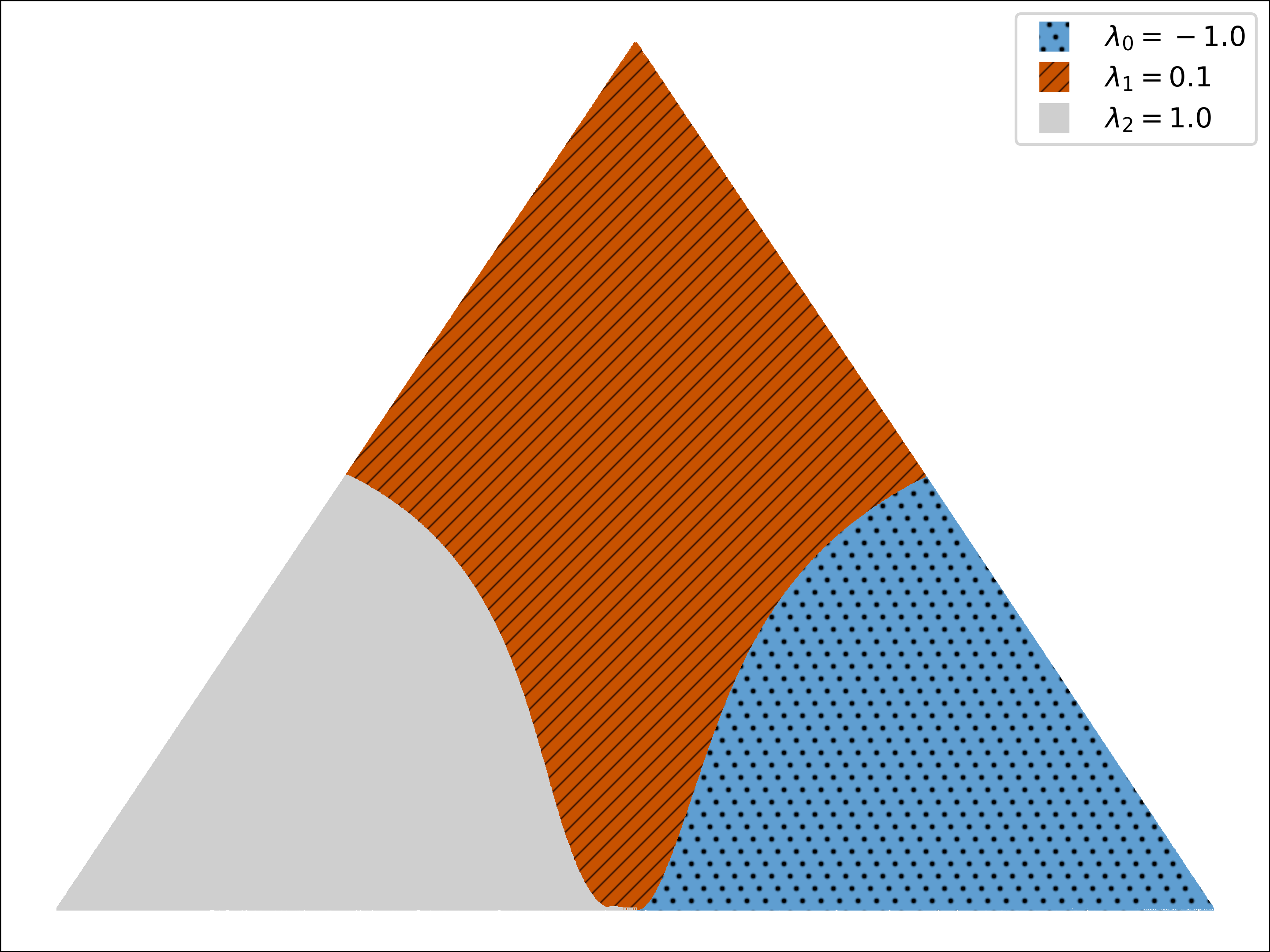
(a) Classic RQI, large gap

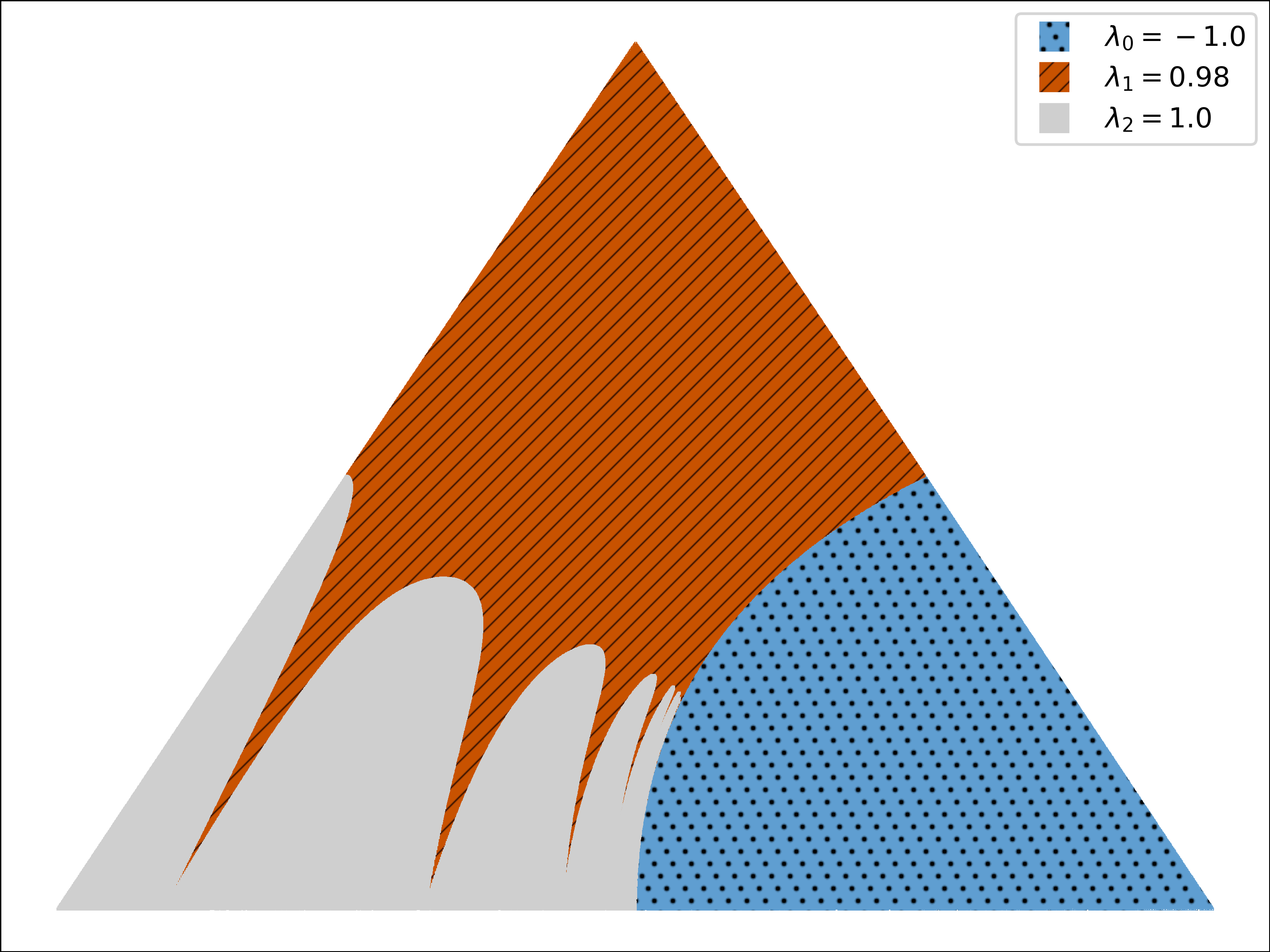
(b) Classic RQI, small gap

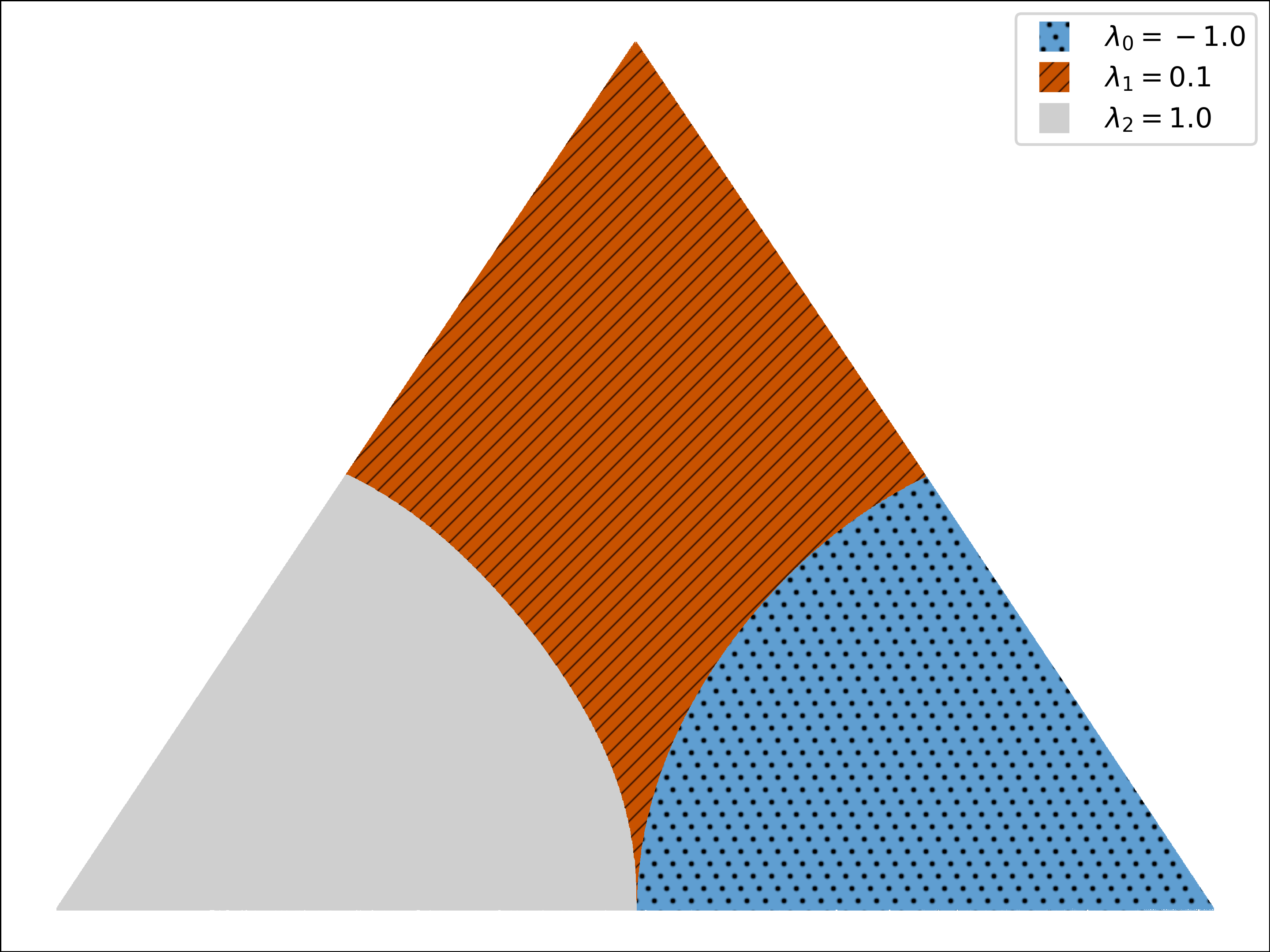
(c) Projected RQI, large gap

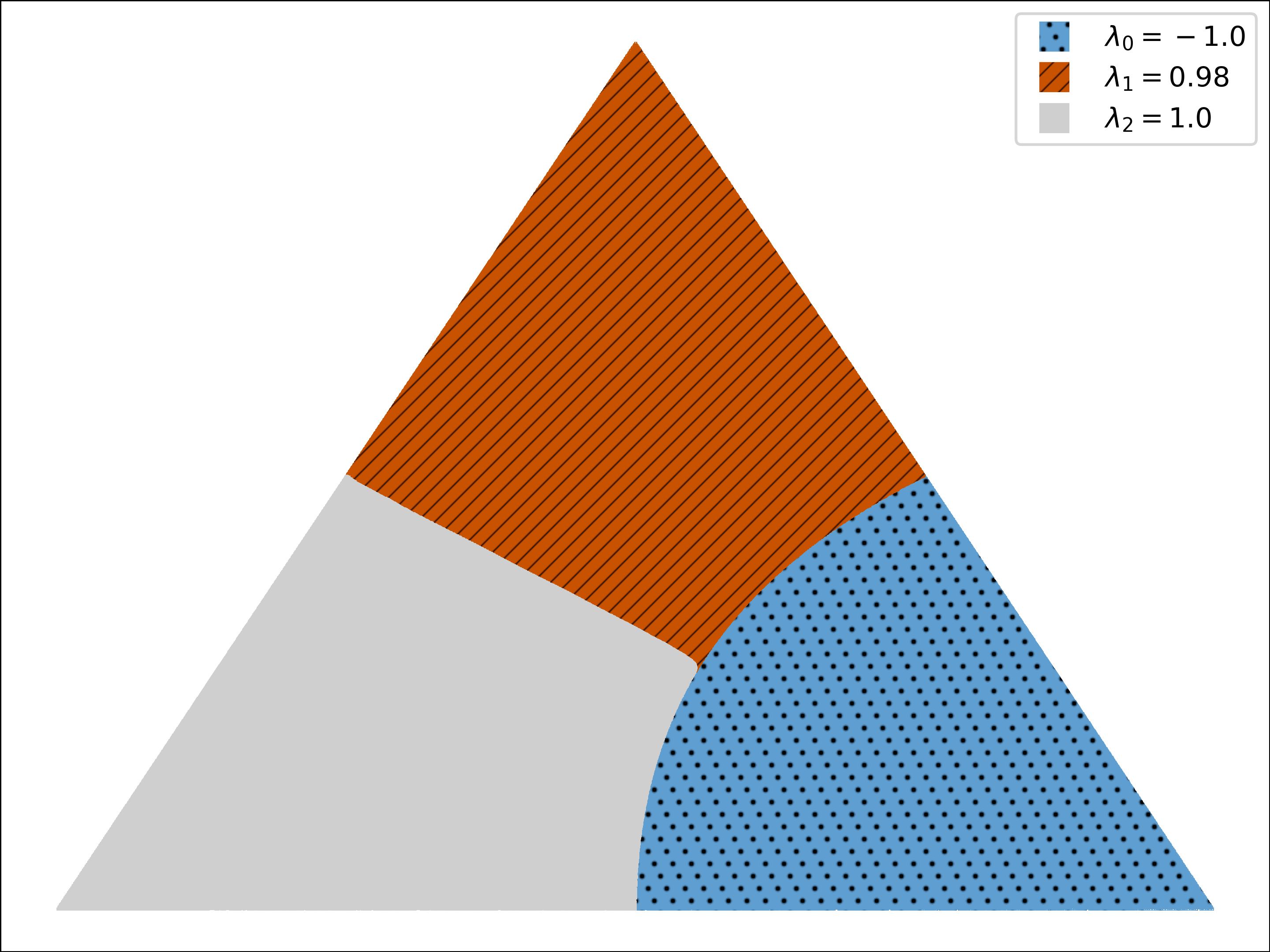
(d) Projected RQI, small gap

Figure 2: Visualisation of the basins of attraction for classic RQI (top row) and PRQI (bottom row) for different eigenvalue gaps in Example 1. If the eigenvalue gap is small (right column), the borders between the basins of attraction deteriorate for classic RQI; for PRQI the border is more regular.

In the first row we observe the well-known behaviour of classic RQI: as the eigenvalue gap gets smaller, the basins of attraction deteriorate. Our method (second row) is more stable and less dependent on the spacing between eigenvalues. In particular, the border between the basins of attraction corresponding to the two closely spaced eigenvalues is more regular, which in practice results in a much more predictable convergence behaviour.

To provide some intuition for these observations, consider $\bm{x}^{(0)}={(\varepsilon\ \tau\ \varepsilon)}^{T}\in\mathbb{R}^{3}$ with $0<\varepsilon\ll 1$ and $0<\tau\approx 1$ such that $\|\bm{x}^{(0)}\|^{2}=2\varepsilon^{2}+\tau^{2}=1$. Then $\bm{x}^{(0)}$ approximates the eigenvector $\bm{v}_{2}={(0\ 1\ 0)}^{T}$ and we have

$$\mu^{(0)}=\frac{{(\bm{x}^{(0)})}^{\ast}A\bm{x}^{(0)}}{{(\bm{x}^{(0)})}^{\ast}\bm{x}^{(0)}}=\tau^{2}s$$

A straightforward calculation then shows that the (unnormalised) iterate after one step of classic RQI is given by

$$\bm{x}^{(1)}={\Big{(}\frac{\varepsilon}{-1-\tau^{2}s}\,,\ \frac{\tau}{(1-\tau^{2})s}\,,\ \frac{\varepsilon}{1-\tau^{2}s}\Big{)}}^{T}.$$

We observe the following: for any $s\in(0,1)$, the first entry of $\bm{x}^{(1)}$ is small because the denominator is bounded away from zero and $\varepsilon\approx 0$. Since $\tau\approx 1$, the denominator of the second entry is small and $\bm{x}^{(1)}$ has a large component in the target direction. The behaviour of the last entry depends on the value of $s$. For a large eigenvalue gap ($s\approx 0$), the last entry is small and $\bm{x}^{(1)}$ is a good approximation of the wanted eigenvalue. If, however, $s\approx 1$, i.e., the eigenvalue gap is small, the denominator of the last entry is small and, depending on how small $\varepsilon$ is, this entry might also blow up. In this case, $\bm{x}^{(1)}$ has a strong component in the direction of the (unwanted) eigenvector $\bm{v}_{3}$. For $s\in(-1,0]$ analogous observations can be made, with the roles of the first

In PRQI, adding the imaginary shift $\gamma=\gamma^{(0)}$ results in

$$\bm{x}^{(1)}={\Big{(}\frac{\varepsilon}{-1-\tau^{2}s-i\gamma}\,,\ \frac{\tau}{(1-\tau^{2})s-i\gamma}\,,\ \frac{\varepsilon}{1-\tau^{2}s-i\gamma}\Big{)}}^{T}.$$

In absolute value, the entries are given by

$$\big{|}x^{(1)}_{1}\big{|} =\frac{\varepsilon}{\sqrt{(1+\tau^{2}s)^{2}+\gamma^{2}}},\ \big{|}x^{(1)}_{2}\big{|}=\frac{\tau}{\sqrt{(1-\tau^{2})^{2}s^{2}+\gamma^{2}}},\ \big{|}x^{(1)}_{3}\big{|}=\frac{\varepsilon}{\sqrt{(1-\tau^{2}s)^{2}+\gamma^{2}}}.$$

In this case, for $s\approx 1$, we have approximately $|x^{(1)}_{2}|\approx\tau/\gamma$ and $|x^{(1)}_{3}|\approx\varepsilon/\gamma$, implying that we do not get a strong component in the direction of the unwanted eigenvector.

Example 2.

Comparing to classic RQI again, we demonstrate in this example for four test matrices that our PRQI method always converges to the correct eigenpair, provided the initial approximation is sufficiently accurate. The test matrices are:

1. The $[1,2,1]$ matrix. This matrix is tridiagonal with all diagonal elements set to $2$ and all off-diagonal elements set to $1$.

2. Wilkinson’s $W_{2n+1}^{+}$ matrix. The $m$th diagonal entry of this tridiagonal matrix is set to $|n+1-m|$ and all off-diagonal entries are set to $1$. This matrix has pairs of very closely spaced eigenvalues, see [25, p. 309].

3. The Laplace matrix, which arises when discretising the Laplacian in 2D using a 5-point stencil with the finite difference method. Let $T$ be a $m\times m$ tridiagonal matrix with $4$ as its diagonal entries and $-1$ on its off-diagonals. The Laplace matrix is a $m^{2}\times m^{2}$ block tridiagonal matrix with $T$ as its diagonal blocks and $-I$ as its off-diagonal blocks, where $I$ is the $m\times m$ identity matrix.

4. Symmetric random matrices with a random (symmetric) sparsity pattern and non-zero entries that are normally distributed with mean $0$ and variance $1$.

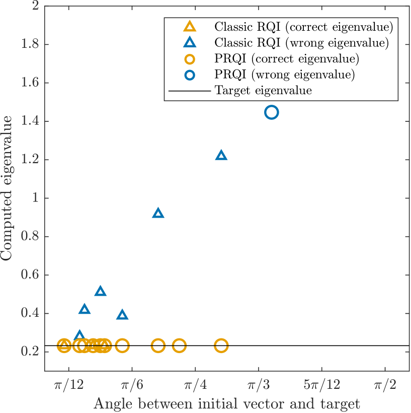
(a) $[1,2,1]$ matrix

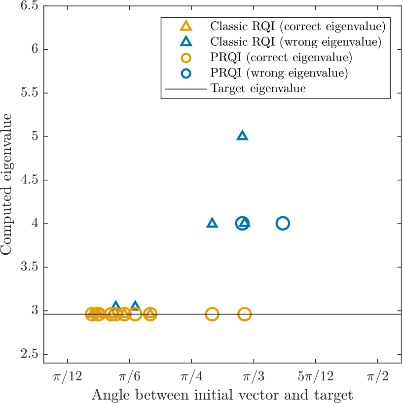
(b) $W_{21}^{+}$ Wilkinson matrix

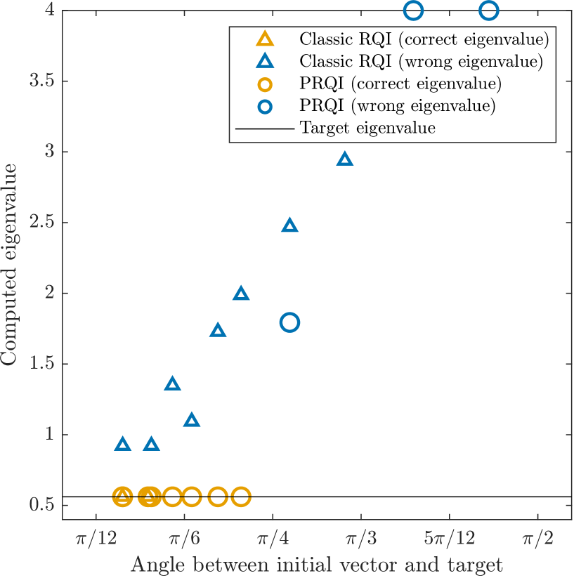
(c) Laplace matrix

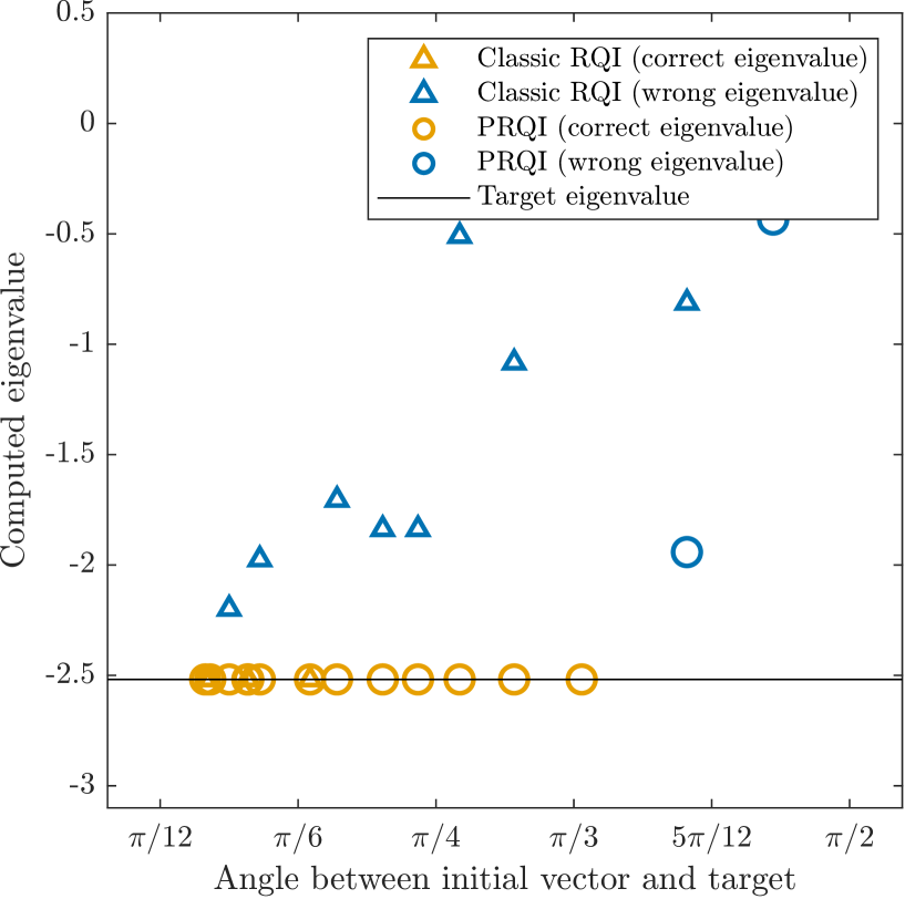
(d) Random matrix

Figure 3: Plot of the angle between the initial vector and the target eigenvector against the computed eigenvalue for the four test matrices in Example 2. The target eigenvalue is depicted by the solid black line. While classic RQI sometimes fails even for very small angles (i.e., very accurate initial vectors), PRQI consistently produces the correct result as soon as the angle is sufficiently small.

The plots in Figure 3 show how the convergence of the classic RQI and PRQI depends on the angle between the initial vector and the target eigenvector. To generate the initial vectors, we first compute the full set of eigenvectors $\{\bm{v}_{1},\dotsc,\bm{v}_{n}\}$ using built-in functions in MATLAB. We then draw $n$ random normally distributed real numbers $\alpha_{j}\sim\mathcal{N}(0,1)$, $j=1,\dotsc,n$, and set $\bm{x}^{(0)}=\sum_{j=1}^{n}\alpha_{j}\bm{v}_{j}$. We randomly select one index $j^{\ast}$ to be the target index and throughout the experiment, we increase $\alpha_{j^{\ast}}$ so that the contribution of $\bm{x}^{(0)}$ in the direction of the target eigenvector $v_{j^{\ast}}$ becomes increasingly bigger (i.e., the angle becomes increasingly smaller).

We observe that PRQI seems to converge to the desired eigenpair once the angle between the initial vector and the target is sufficiently small. Classic RQI, on the other hand, still often converges to the wrong eigenpair for small initial error angles. In other words, our modification of classic RQI does indeed yield a method that makes more use of the initial vector instead of the initial shift.

Example 3.

For this example we consider the following Sturm–Liouville problem

$$-u^{\prime\prime}(x)+\left(\sin x-\frac{40}{1+x^{2}}\right)u(x) =\lambda u(x),\qquad x\in(0,\infty)\,,$$ (4.2)

$$u(0) =0\,,$$

which exhibits a band-gap structure and also has “trapped” discrete eigenvalues in the gaps. These types of spectral problems arise, e.g., in the modelling of photonic crystal fibres [16], and the specific problem above has been studied previously in [2, 17, 18]. Our goal is to compute some of the eigenvalues in the gaps, which will be complicated by the following two facts: (1) the discrete eigenvalues in the gaps accumulate at the lower end of the bands; and (2) naïve numerical discretisation of (4.2) generates additional, unwanted (so-called spurious) eigenvalues in the spectrum within close distance to and thus indistinguishable from the target eigenvalues. Nevertheless, since the eigenvectors have known distinct structures, PRQI is well suited to computing eigenvalues lying in one of the lower spectral gaps while avoiding convergence to a spurious eigenvalue. Since our main goal is to show that PRQI converges to one of the target eigenvalues using only coarse a priori information about the shape of the target eigenvector, we use a simple discretisation. To compute eigenvalues in higher spectral gaps, a discretisation with higher accuracy is required, since the accuracy of the eigenvalues of the discretised problem quickly deteriorates when going to higher parts of the spectrum [2].

Let us first describe the problem and the numerical discretisation more carefully. As mentioned above, the operator in (4.2) has band-gap structure with very closely spaced, discrete eigenvalues in the gaps accumulating at the lower ends of the bands (see [18] or [11, Chap. 4-5] for details). The first two bands are given by

$$J_{1}=[-0.37849,-0.34767],\ J_{2}=[0.59480,0.91806]\,,$$ (4.3)

and our goal is to compute some of the discrete eigenvalues in the gap between those bands. We will exploit the fact that the qualitative behaviour of the desired eigenfunctions is very different from that of the undesired ones. As depticted in Figure 4, the target eigenfunctions decay exponentially away from the left boundary while the eigenfunctions corresponding to spurious eigenvalues decay exponentially away from the right boundary, see [18].

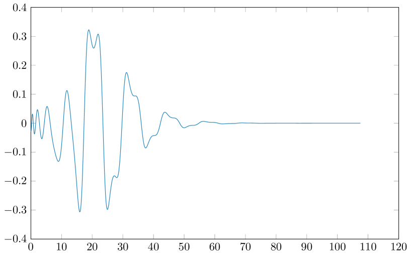
(a) Target eigenfunction

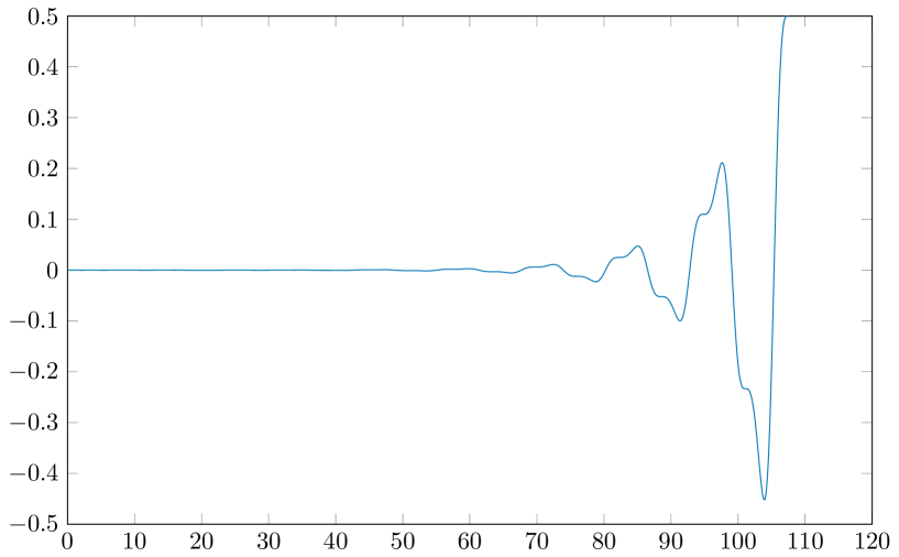
(b) Eigenfunction of spurious eigenvalue

Figure 4: Plots of one of the eigenfunctions corresponding to a target eigenvalue (left) and of the eigenfunction corresponding to an unwanted, spurious eigenvalue (right) for the Sturm-Liouville problem in (4.2).

To solve (4.2) numerically, we discretise the equation using the finite element method, see, e.g.,  [10]. First, the problem is truncated to the interval $[0,X]$, for $X>0$ sufficiently large, where at the artificial boundary we impose a Neumann boundary condition $u^{\prime}(X)=0$. The weak formulation of the resulting problem, obtained by multiplying with a test function $\varphi\in V\coloneqq\{f\in H^{1}([0,X])\mid f(0)=0\}$ and integrating by parts reads: Find $u\in V$ such that with $q(x)\coloneqq\sin x-{40}/{(1+x^{2})}$ we have

$$\int_{0}^{X}u^{\prime}\varphi^{\prime}+\int_{0}^{X}qu\varphi=\lambda\int_{0}^{X}u\varphi\,,\qquad\text{for all }\varphi\in V.$$ (4.4)

Let now $V_{h}\subset V$ be the space of piecewise linear finite elements with respect to the uniform mesh $\{0=x_{1}<\dotsm<x_{n}=1\}$ with (Lagrange) basis $\{\varphi_{1},\dotsc,\varphi_{n}\}$ such that $\varphi_{j}(x_{i})=\delta_{ij}$ for all $i,j\leq n$. For the meshwidth $h=x_{k+1}-x_{k}$, for all $k$, we used $h=0.01$. Replacing $u$ in (4.4) by a function $u_{h}\in V_{h}$ and expanding in the basis such that $u_{h}=\sum_{j=1}^{n}v_{j}\varphi_{j}$ leads to an algebraic eigenvalue equation of the form

$$(A+B)\bm{v}=\lambda M\bm{v}\,,$$ (4.5)

with $\bm{v}={(v_{1},\dotsc,v_{n})}^{T}$ and the entries of the matrices $A,B,M\in\mathbb{R}^{n\times n}$ are given by

$$A_{ij}=\int_{0}^{X}\varphi_{i}^{\prime}\varphi_{j}^{\prime}\,,\qquad B_{ij}=\int_{0}^{X}q\varphi_{i}\varphi_{j}\,,\qquad M_{ij}=\int_{0}^{X}\varphi_{i}^{\prime}\varphi_{j}^{\prime}\,.$$

In Figure 5 we plot a close-up of the spectrum of the original and the perturbed problem respectively around the target eigenvalues (cf. Figure 1). The marked eigenvalue is the spurious one; the eigenvalues left and right of it are two of the target eigenvalues. The perturbed spectrum corresponds to the eigenproblem

$$(A+B+i(M-M\bm{x}_{0}{(M{\bm{x}_{0}})}^{T}))\bm{v}=\lambda M\bm{v}\,,$$

where $\bm{x}_{0}\in\mathbb{R}^{n}$ is the initial vector used in PRQI, described below.

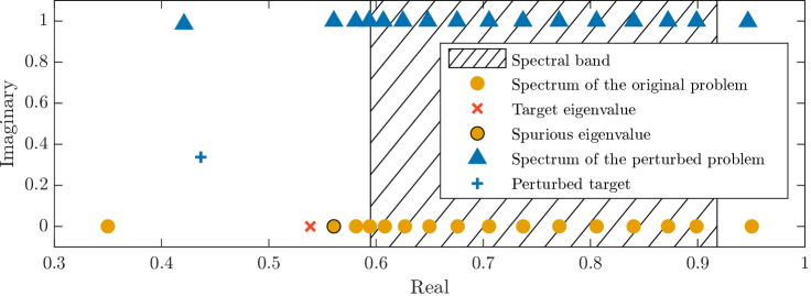
Figure 5: Part of the spectrum of the original and the perturbed Sturm-Liouville eigenvalue problem (4.2). The target eigenvalue in the original spectrum (red cross) is very close to the unwanted eigenvalues in the band (hatched region) and the spurious eigenvalue (bordered circle). The perturbed eigenvalues (blue triangles) are raised into the complex plane and only the target eigenvalue (blue cross) stays near the real line.

Recall that the eigenfunctions corresponding to target eigenvalues are exponentially decaying, and, being eigenfunctions of a Sturm–Liouville operator, are also oscillating. As such, we generate the initial vectors $\bm{x}_{0}$ discretising and normalising (w.r.t. the $\|\cdot\|_{M}$ norm) functions $f:[0,X]\rightarrow\mathbb{R}$ that are constructed as follows:

1. Choose a cutoff value $R\in(0,X)$.

2. For $x>R$ set $f(x)=0$ (this cutoff models the exponential decay).

3. For $x\leq R$ define $f$ to be piecewise constant and oscillating, taking values $\pm 1$.

Due to the Dirichlet boundary condition at $x=0$ we further set $f(x)=0$ on $[0,x_{0}]$ for some small $x_{0}>0$. Throughout our experiments we used $x_{0}=0.1$. Figure 6(a) shows an initial vector generated by this approach for a cutoff value of $R=35$ (which is approximately a third of the total length of the interval). Below we will vary the number of oscillations $n_{\text{osc}}$ for fixed $R$; since the oscillatory part of the function $f$ used to generated this vector consisted of three full oscillations before setting it to zero on $[0,x_{0}]$, we say that this vector corresponds to $n_{\text{osc}}=3$.

Figures 6(b) and 6(c) are the eigenvectors computed by PRQI and classic RQI, respectively using this initial vector. PRQI converged to the target eigenvalue $\lambda_{\text{PRQI}}=0.53874$ (which is in the gap between the bands $J_{1}$ and $J_{2}$ in (4.3)), while classic RQI converged to an eigenvalue far away ($\lambda_{\text{RQI}}=26.8648$). For classic RQI to converge to a value in the first spectral gap it was necessary to also set the initial shift appropriately.

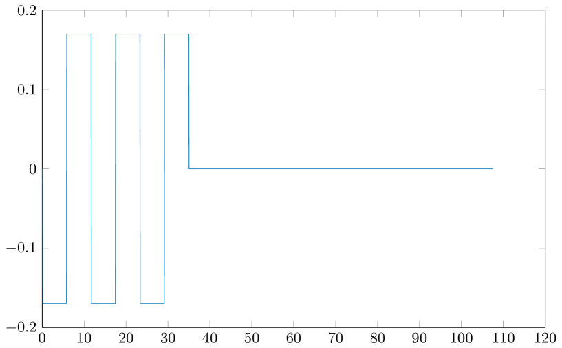
(a) Initial vector

(b) PRQI result

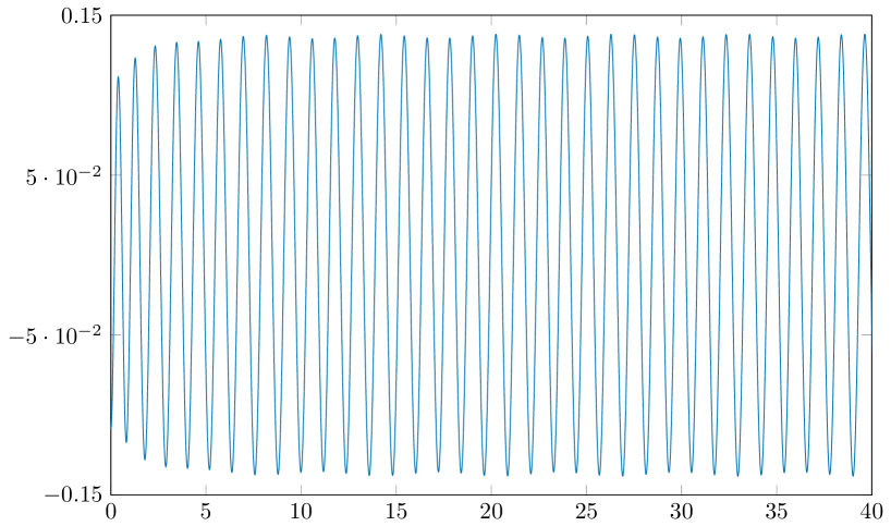
(c) Classic RQI result

Figure 6: The left figure shows an initial vector used to compute an eigenpair of (4.2) in the second spectral gap with PRQI. The middle figure is the eigenvector that PRQI converged to. The right figure shows the eigenvector computed by classic RQI (we cropped the interval at $x=40$ for better visualisation).

To target other eigenvalues in the first spectral gap, we can vary $R$ and/or $n_{\text{osc}}$. While PRQI succesfully avoided convergence to a spurious eigenvalue in all our experiements, it sometimes converged to an eigenvalue in one of the spectral bands. Since these eigenvalues correspond to the essential spectrum of the original problem, the computed eigenvectors are not localized anywhere, i.e., they oscillate over the whole interval $[0,X]$. This allows us to implement a modified PRQI that early on detects convergence to an unwanted eigenvalue. Let $S\in[0,X]$ and define

$$\eta(\bm{x}^{(k)})=\frac{\|\bm{x}^{(k)}\mathds{1}_{\{x>S\}}\|}{\|\bm{x}^{(k)}\|}\in[0,1]\,,$$

where $\bm{x}^{(k)}$ is the current vector iterate and $\bm{x}^{(k)}\mathds{1}_{\{x>S\}}\in\mathbb{C}^{n}$ is a vector constructed from $\bm{x}^{(k)}$ by setting all entries at indices corresponding to function values at $x\leq S$ to zero. For $S$ sufficiently large, vectors corresponding to target eigenvalues, being exponentially decaying, will satisfy $\eta(\bm{x}^{(k)})\ll 1$. Thus, to detect convergence to an unwanted eigenvector, during each iteration of PRQI we can check if $\eta(\bm{x}^{(k)})>\eta^{\ast}$ for some threshold value $\eta^{\ast}$ and if yes, abort the current execution (a similar criterion is proposed in [13, 19]). We used $S=80$ and determined $\eta^{\ast}$ by computing $\eta$ for a rapidly oscillating sine function. This gave $\eta\approx 0.5$, so we choose $\eta^{\ast}=0.4$.

Table 1 summarises the results using this approach for a few exemple values of $n_{\text{osc}}$ and $R$, the number of oscillations and cutoff values of the initial vectors that we used. The column “Index” contains the index of the eigenvalue computed by the respective method within the spectrum of the discretised equation (4.5) counted from the smallest eigenvalue.

		PRQI			Classic RQI
$n_{\text{osc}}$	$R$	Eigenvalue	Index	# Its.	Eigenvalue	Index	# Its.
1.5	35	-0.227061	22	7	25.063959	174	8
2	35	0.349875	23	8	36.440082	209	6
2.5	35	0.538745	24	8	43.496076	228	6
3	55	0.349875	23	7	34.340555	203	7
3.5	55	0.538745	24	7	46.251764	235	4
4	55	0.581339	26	7	45.060462	232	7

Table 1: Results of applying PRQI and classic RQI to the Sturm–Liouville problem for different initial vectors parametrised by the number of oscillations $n_{\text{osc}}$ and the cutoff value $R$ . PRQI converged to one of the target eigenvalues for many different combinations of $n_{\text{osc}}$ and $R$ while classic RQI always converged to an eigenvalue far away. Furthermore, PRQI successfully skips the spurious eigenvalue $\lambda_{\text{sp}}\approx 0.56$ with Index 25, and it required on average only one iteration more than classic RQI.

We observe that PRQI converges to a target eigenvalue for many different initial vectors and on average requires only one iteration more than classic RQI, while classic RQI consistently converges to an eigenvalue very far away.

The results obtained for classic RQI can be explained by computing the Rayleigh quotient for the initial vectors used. For instance, the Rayleigh quotient for the initial vector $\bm{x}^{(0)}$ corresponding to the values in the first row is given by $\mathcal{R}(\bm{x}^{(0)})\approx 24.7$. In practice, however, one would rarely use classic RQI directly for this problem and certainly not with such a bad shift. The endpoints of the spectral gaps can be computed using Floquet theory [11], and one would therefore instead use some value inside the spectral gap in which the eigenvalue is sought as the initial shift in classic RQI. Usually a few iterations with a fixed shift (i.e., with the shifted inverse iteration) are carried out before switching to the Rayleigh quotient shift. However, as demonstrated in Example 1, classic RQI is strongly dependent on the value of the initial shift and so this approach is not suitable for this type of problem.

To demonstrate this, we carried out some further tests: Without any further information, one reasonable choice for the initial shift would be the midpoint of the first spectral gap $\mu^{(0)}\approx 0.1236$. However, we found that classic RQI (both when preceded by inverse iteration and when used stand-alone) usually converges to an eigenvalue close to the shift, in this case either to the eigenvalue $0.349875$ or $-0.227061$. To target the eigenvalues near the right end of the gap, we also used $\mu^{(0)}=0.5$ as the initial shift. This, however, caused convergence to the unwanted spurious eigenvalue for some combinations of $R$ and $n_{\text{osc}}$ (e.g., $R=35$, $n_{\text{osc}}=4$).

5 Conclusion

In this paper we have presented a modification of the classic Rayleigh Quotient Iteration with the aim to produce a method that overcomes some of the problems of RQI. The method, which we called Projected RQI (PRQI), was first introduced by perturbing the matrix using the projection onto the orthogonal complement of the initial vector and using this matrix during the iteration in RQI. We then showed that this approach can be simplified: it suffices to add an imaginary shift to the Rayleigh quotient shift in RQI.

We then proved that PRQI is cubically convergent and we presented numerical examples that demonstrate that the convergence behaviour of PRQI is indeed more robust than that of classic RQI. In particular, PRQI seems to make more use of the information in the initial vector instead of the initial shift. We then showed how this behaviour can be used to compute certain eigenvalues in a band-gap spectrum of a Sturm–Liouville operator. It was demonstrated how a small amount of a priori knowledge about the shape of an eigenvector can be used to construct an initial vector that precludes the convergence of PRQI to unwanted eigenpairs.

As we have remarked after the proof of Theorem 3.2, the convergence result that we proved is in a certain sense too weak. In particular, it can not explain the improved behaviour observed in the numerical examples. One direction for future research would therefore be to improve the convergence theorem; in the discussion following the current proof we already remarked that this likely requires a more accurate estimation of the eigenvalues of the matrix ${A}-i\gamma^{(k)}\bm{x}^{(k)}{(\bm{x}^{(k)})}^{\ast}I$.

Other possible avenues for future work would be to consider more examples of the Sturm–Liouville type as in Example 3. In [24] classic RQI and Inverse Iteration are combined to confine the eigenvalue iterates to a given interval. In the Sturm–Liouville example, the endpoints of the spectral gaps can be computed using Floquet theory [11], so possibly the idea in [24] can be extended to include PRQI: the combination of classic RQI and Inverse Iteration would ensure that the resulting eigenvalue lies within the wanted gap while PRQI avoids convergence to a spurious eigenvalue. Combining classic RQI and PRQI could also be fruitful in other cases as a means to improve convergence speed by switching from PRQI to classic RQI (i.e., setting $\gamma=0$) once the error residual is sufficiently small.

Acknowledgments. Many thanks go to Chris Hart for the excellent foundations he laid for this paper more than 12 years ago and to Marco Marletta for the many useful suggestions during that period. This work is supported by Deutsche Forschungsgemeinschaft (German Research Foundation) under Germany’s Excellence Strategy EXC 2181/1 - 390900948 (the Heidelberg STRUCTURES Excellence Cluster).

References

- [1] P.-A. Absil, R. Sepulchre, P. Van Dooren, and R. Mahony. Cubically convergent iterations for invariant subspace computation. SIAM J. Matrix Anal. Appl., 26(1):70–96, 2004.
- [2] L. Aceto, P. Ghelardoni, and M. Marletta. Numerical computation of eigenvalues in spectral gaps of Sturm–Liouville operators. J. Comput. Appl. Math., 189(1):453–470, 2006.
- [3] R. Altmann, P. Henning, and D. Peterseim. Quantitative Anderson localization of Schrödinger eigenstates under disorder potentials. Math. Models Methods Appl. Sci., 30(5):917–955, 2020.
- [4] R. Altmann and D. Peterseim. Localized computation of eigenstates of random Schrödinger operators. SIAM J. Sci. Comput., 41(6):B1211–B1227, 2019.
- [5] D. N. Arnold, G. David, M. Filoche, D. Jerison, and S. Mayboroda. Computing spectra without solving eigenvalue problems. SIAM J. Sci. Comput., 41(1):B69–B92, 2019.
- [6] S. Batterson and J. Smillie. The dynamics of Rayleigh Quotient Iteration. SIAM J. Numer. Anal., 26(3):624–636, 1989.
- [7] C. Beattie and D. W. Fox. Localization criteria and containment for Rayleigh Quotient Iteration. SIAM J. Matrix Anal. Appl., 10(1):80–93, 1989.
- [8] J. Berns-Müller, I. G. Graham, and A. Spence. Inexact inverse iteration for symmetric matrices. Linear Algebra Appl., 416(2):389–413, 2006.
- [9] S. Börm and C. Mehl. Numerical Methods for Eigenvalue Problems. De Gruyter, Berlin, 2012.
- [10] D. Braess. Finite Elements: Theory, Fast Solvers, and Applications in Solid Mechanics. Cambridge University Press, 2007.
- [11] B. M. Brown, M. S. Eastham, and K. M. Schmidt. Periodic Differential Operators, volume 230 of Oper. Theory Adv. Appl. Birkhäuser/Springer, Basel, 2013.
- [12] G. H. Golub and C. F. Van Loan. Matrix Computations. The John Hopkins University Press, Baltimore, third edition, 1996.
- [13] D. S. Grebenkov and B.-T. Nguyen. Geometrical structure of Laplacian eigenfunctions. SIAM Rev., 55(4):601–667, 2013.
- [14] W. W. Hager. Updating the inverse of a matrix. SIAM Rev., 31(2):221–239, 1989.
- [15] R. A. Horn and C. R. Johnson. Matrix Analysis. Cambridge University Press, 2012.
- [16] P. Kuchment. The Mathematics of Photonic Crystals. In G. Bao, L. Cowsar, and W. Masters, editors, Mathematical Modeling in Optical Science, Frontiers in Applied Mathematics, pages 207–272. SIAM, Philadelphia, 2001.
- [17] M. Marletta. Neumann–Dirichlet maps and analysis of spectral pollution for non-self-adjoint elliptic PDEs with real essential spectrum. IMA J. Numer. Anal., 30(4):917–939, 2010.
- [18] M. Marletta and R. Scheichl. Eigenvalues in spectral gaps of differential operators. J. Spectr. Theory, 2(3):293–320, 2012.
- [19] J. S. Ovall and R. Reid. An algorithm for identifying eigenvectors exhibiting strong spatial localization. Math. Comp., 92:1005–1031, 2023.
- [20] R. D. Pantazis and D. B. Szyld. Regions of convergence of the Rayleigh Quotient Iteration method. Numer. Linear Algebra Appl., 2(3):251–269, 1995.
- [21] B. N. Parlett. The Rayleigh Quotient Iteration and some generalizations for nonnormal matrices. Math. Comp., 28(127):679–693, 1974.
- [22] B. N. Parlett. The Symmetric Eigenvalue Problem. Classics in Applied Mathematics. SIAM, Philadelphia, 1998.
- [23] Y. Saad. Numerical Methods for Large Eigenvalue Problems. Classics in Applied Mathematics. SIAM, Philadelphia, second edition, 2011.
- [24] D. B. Szyld. Criteria for combining Inverse and Rayleigh Quotient Iteration. SIAM J. Numer. Anal., 25(6):1369–1375, 1988.
- [25] J. H. Wilkinson. The Algebraic Eigenvalue Problem. Monographs On Numerical Analysis. Clarendon Press, Oxford, 1965.