A Framework for Exploring Nuclear Physics Sensitivity in Numerical Simulations

Abstract

We describe the AMReX-Astrophysics framework for exploring the sensitivity of astrophysical simulations to the details of a nuclear reaction network, including the number of nuclei, choice of reaction rates, and approximations used. This is explored by modeling a simple detonation with the Castro simulation code. The entire simulation methodology is open-source and GPU-enabled.

1 Introduction

Nucleosynthesis is the process of forming new atomic nuclei via nuclear reactions. By studying both stellar and primordial nucleosynthesis, we gain better insights into stellar evolution, the chemical evolution of galaxies, and the element composition of the Universe. Moreover, enormous amounts of energy are released during nuclear fusion reactions in stellar nucleosynthesis, which is the power source leading to thermonuclear explosions such as Type Ia supernovae (SN Ia) [1, 2] and X-ray bursts (XRBs) [3]. Given the wide range of astrophysical environments in which nucleosynthesis occurs, each characterized by distinct thermodynamic conditions and dynamics, nuclear reaction networks are generally tailored to each case.

Due to limited computational resources, simulations of astrophysical explosions often use small to moderate-sized networks. Generally, the number of isotopes and reaction rates that can be included depends on the dimensionality of a simulation. In 1D, it is possible to incorporate more than a thousand isotopes along with thousands of nuclear reaction rates [4]. However, the situation becomes significantly more challenging in 2- and 3D, due to the increased memory and the need to advect each species separately. A contemporary 2D XRB simulation can include 25 isotopes easily [5], while a 3D XRB simulation can be restricted to $\sim 10$ isotopes [6, 7].

A reaction sensitivity study is essential to assess the reliability of a simulation where reactions provide a significant part of the energy budget. This can explore the significance of each individual reaction rate, the size of the network, the modifications to rates (like screening), and approximations used in the network. For example, through a sensitivity study, we can identify the most critical reaction rates that should be included in the network while eliminating unimportant ones to reduce cost. During this process, we also gain insights into how reaction rates impact the properties of the problem, such as the propagating speed of a thermonuclear flame in an XRB [5] and the light curve of thermonuclear explosions, leading to a better convergence between the numerical models and observations.

Here we present the AMReX-Astrophysics / pynucastro framework for exploring nuclear reaction physics in numerical simulations. The reaction networks are generated via the pynucastro library [8, 9], which writes GPU-enabled C++ networks for use in the AMReX-Astrophysics Microphysics library [10]. In section 2, we describe the overall procedure and workflow for generating an arbitrary reaction network with its right-hand-side (RHS) and Jacobian using pynucastro. In section 3, we demonstrate a simple sensitivity study using the compressible hydrodynamics code Castro [11, 12] to model a 1D ${}^{4}\mathrm{He}$ detonation. All of these codes are developed openly and are freely available on GitHub.

2 Arbitrary Network Generation

The first step in a reaction sensitivity study is the generation of the reaction network. We will use pynucastro for this purpose. pynucastro is a Python library that allows users to interactively explore nuclear reaction rates, construct any arbitrary reaction network, and export the RHS and Jacobian for the network for use in an integrator. The ReacLibLibrary class provides access to the collection of JINA ReacLib [13] rates and the TabularLibrary class provides tabulated weak rates from various sources [14, 15]. A detailed description of pynucastro can be found in [9], here we only emphasize essential points related to network generation.

To illustrate the process of network generation, we start by explaining the design philosophy and steps involved in building the subch_simple network, a network employed in our prior research studies [5, 16]. Subsequently, we showcase how this methodology can be seamlessly extended to develop more complex networks.

The first step in the network generation process is selecting the nuclei of interest. We will build a network that is appropriate for He burning in a detonation. Both ReacLibLibrary and TabularLibrary provide a method called linking_nuclei() that takes a list of nuclei as input and returns a Library object with all possible rates that connect the input nuclei. This is demonstrated in the following code:

⬇

import pynucastro as pyna

# Create a library object that contains all ReacLib rates

reaclib_lib = pyna.ReacLibLibrary()

# Create a list of nuclei

nuc_list = ["p", "he4", "c12", "o16", "ne20", "mg24", "si28",

"s32", "ar36", "ca40", "ti44", "cr48", "fe52", "ni56",

"al27", "p31", "cl35", "k39", "sc43", "v47", "mn51",

"co55", "n13", "n14", "f18", "ne21", "na22", "na23"]

# Returns a subset of ReacLib Library

subch_lib = reaclib_lib.linking_nuclei(nuc_list)

Next, various fine-tuning procedures can be done on this Library to reduce the overall size of the network. It is often desirable to manually remove rates that have been determined as insignificant for energy generation or nucleosynthesis based on past studies. This can be accomplished using Library built-in method remove_rate() by supplying either the Rate object or the short name of the rate in the form of a string: "A(x, y)B". Below we demonstrate this by removing the reverse rates of C and O reactions as well as some links involving heavy nuclei:

⬇

for r in subch_lib.get_rates():

# Check if the products of the rate are the following

if sorted(r.products) in [[pyna.Nucleus("c12"), pyna.Nucleus("c12")],

[pyna.Nucleus("c12"), pyna.Nucleus("o16")],

[pyna.Nucleus("o16"), pyna.Nucleus("o16")]]:

# Remove the rate

subch_lib.remove_rate(r)

# A list of rates to remove by simply supplying the short-name of the rate

rates_to_remove = ["p31(p,c12)ne20", "si28(a,c12)ne20",

"ne20(c12,p)p31", "ne20(c12,a)si28",

"na23(a,g)al27", "al27(g,a)na23",

"al27(a,g)p31", "p31(g,a)al27"]

# Remove rates individually from the network

for r in rates_to_remove:

subch_lib.remove_rate(r)

We can also directly modify the products of a reaction, to further simplify the network. This is useful, for example, in a neutron-capture sequence like A(B, n)Y(n, $\gamma$)C where the neutron capture on Y is significantly faster than the first reaction. In this case, a simple approximation involves modifying the product of the first rate to yield the final product of the two-reaction sequence, C, while retaining the rate of the first reaction and adjusting the overall Q-value accordingly. This is demonstrated in the following code:

⬇

# Select the reaction rates and end product to modify

modify_rates = [("c12(c12,n)mg23", "mg24"),

("o16(o16,n)s31", "s32"),

("o16(c12,n)si27", "si28")]

for r, mp in modify_rates:

# Get the specifc Rate object using the short-name

_r = reaclib_lib.get_rate_by_name(r)

# Modify the product of that rate

_r.modify_products(mp)

# Add the modified rate into the customized Library.

subch_lib.add_rate(_r)

This network describes $\alpha$-captures up to the iron group (and is the starting point for the subch_simple network from [5]). However, for modeling SN Ia, the formation of iron-peak isotopes via electron capture during the explosion is important [17, 18, 19, 20]. We can include these by adding tabulated weak rates. The code below obtains a new set of rates from both ReacLibLibrary and TabularLibrary in the iron-peak and combines them with our existing rates to create our custom rate library all_lib. Note that while the original set of nuclei did not include neutrons, we do include neutrons in the iron-group reactions.

⬇

# Define a new set of nuclei describing iron peak rates

iron_peak = ["n", "p", "he4", "mn51", "mn55",

"fe52", "fe53", "fe54", "fe55", "fe56",

"co55", "co56", "co57", "ni56", "ni57", "ni58",

"cu59", "zn60"]

# Get a subset library with reaclib rates associated with these nuclei

iron_reaclib = reaclib_lib.linking_nuclei(iron_peak)

# Create the library that contains tabulated weak rates from Langanke

# and create a subset library with the rates associated with these nuclei

weak_lib = pyna.TabularLibrary()

iron_weak_lib = weak_lib.linking_nuclei(iron_peak)

# Combine all three libraries together.

all_lib = subch_lib + iron_reaclib + iron_weak_lib

There may be duplicated weak rates from the ReacLib library and the tabulated weak rates. To avoid errors when creating the network, these duplicates can be identified and removed via the find_duplicated_links() method:

⬇

# Find the duplicated links

dupes = all_lib.find_duplicate_links()

rates_to_remove = []

# Remove the ReacLibRate version in duplicates

for d in dupes:

for r in d:

if isinstance(r, pyna.rates.ReacLibRate):

rates_to_remove.append(r)

# Remove rates

for r in rates_to_remove:

all_lib.remove_rate(r)

After we’ve completed the construction of the customized rate libraries, pynucastro can output functions to compute both the righthand-side (RHS) of the ODE system of evolution equations and the Jacobian matrix. Several formats are possible, each provided by a different class: PythonNetwork for Python, SimpleCxxNetwork for a basic C++ network, and AmrexAstroCxxNetwork for C++ for use in the AMReX-Astrophysics suite. For our simulations, we want an AmrexAstroCxxNetwork, which can be used with Castro, and couples with hydrodynamics through a variety of integration techniques (e.g., our simplified-SDC method [21]). We create a network in this format simply as:

⬇

# Use previously defined customized library to create our network

net = pyna.AmrexAstroCxxNetwork(libraries=[all_lib])

Finally, pynucastro can also approximate rate sequences like A$(\alpha,\mbox{p})$X(p,$\gamma$)B rates into an effective as A$(\alpha,\gamma)$B rate, which is used in the traditional “aprox” [22] networks. This approximation holds valid when the proton-capture rate happens at a much faster timescale compared to the ($\alpha$, p) rate, causing an overall equilibrium in the proton flow. Similar to modify_products(), this approximation reduces the size of the network by removing the intermediate nuclei. This method is demonstrated in the following code:

⬇

# Perform the (a,p)(p,g) approximation by specifying the intermediate nuclei

net.make_ap_pg_approx(intermediate_nuclei=["cl35", "k39", "sc43", "v47"])])

# Remove intermediate nuclei since now they’re approximated out

net.remove_nuclei(["cl35", "k39", "sc43", "v47"])])

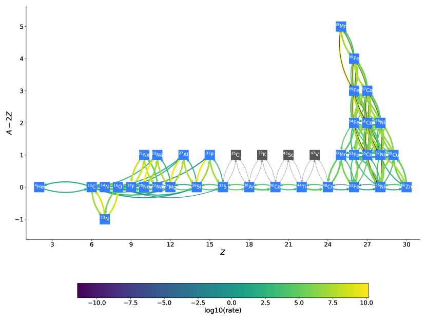
Our final network has 36 isotopes and 149 rates including 12 TabularRate rates (compared to the original subch_simple with 22 isotopes and 57 rates). Note that subch_simple also uses the ($\alpha$, p)(p, $\gamma$) approximation for ³⁵Cl, ³⁹K, ⁴³Sc, ⁴⁷V, ⁵¹Mn, and ⁵⁵Co. Before writing out the actual RHS and the Jacobian, there are also methods that allow the user to explore the network they created and make adjustments if needed. For example, there is an easy interface to plot each reaction rate with a specified density, temperature, and mass abundances that mimic the simulation conditions to help determine the importance of each rate. An example output of the built-in plotting functions is shown in Figure 1.

Figure 1: A visualization of the custom network that we created using the pynucastro package. The color bar shows the reaction rates with solar composition, $\rho=9\times 10^{7}$ g $\mathrm{cm}^{-3}$, and $T=6\times 10^{9}$ K. The horizontal axis and the vertical axis show the atomic number, $Z$, and the extra number of neutrons compared to the number of protons, respectively. The gray nodes with dotted gray lines represent the $(\alpha,\mbox{p})(\mbox{p},\gamma)$ approximation, which are not directly in the network. All reactions that have the form, $A(X,\alpha)B$ or $A(\alpha,X)B$, are hidden for better clarity.

Once we’re satisfied with the current network, pynucastro can write out all the necessary files, including the RHS and the Jacobian of the network, compatible with Microphysics and Castro with a single function:

⬇

# Write all files needed by the package, Microphysics, to integrate the network

net.write_network()

The AMReX-Astrophysics Microphysics library contains all of the code needed to support the integration of this network, including an equation of state (we’ll use the Helmholtz EOS from [23]), integrators such as VODE [24], as well as routines for neutrino cooling and plasma screening. Microphysics can be used on its own to perform network evolution with self-heating or coupled to a simulation code, like Castro. It provides the necessary interfaces to support several different methods of coupling hydrodynamics and reactions.

Typically, a user creates a dedicated directory in Microphysics under Microphysics/networks (we’ll use custom_net for the network described above). This directory serves as the repository containing both the network-generating script using pynucastro and all the associated auto-generated files.

3 Network Sensitivity Testing

We will now show how to do a network sensitivity study similar to the one recently performed for XRBs in [5]. Any Castro problem setup can be told to use our new network (in the Microphysics directory hierarchy) at compile time, via:

⬇

make NETWORK_DIR=custom_net

To demonstrate a simple sensitivity testing, we use the Detonation test problem in Castro. Detonation models a 1D propagating detonation wave, offering a way to replicate the thermodynamic conditions of the He detonation wave found in the shell-burning stage of the sub-Chandrasekhar double-detonation model [25], as discussed in previous work [21, 16]. This sensitivity testing on the Detonation problem helps us choose the appropriate network for a realistic sub-Chandrasekhar double-detonation model, especially when studying nucleosynthesis.

To demonstrate this idea, we will compare subch_simple and the classic 19-isotope network, aprox19 [26], with the network we generated in Section 2, which will be referred to as He-C-Fe. Our detonation simulation spans a domain up to $x=4.0\times 10^{7}$ cm, with 256 coarse grid zones. By employing two refinement levels with ratios of 2, we reach 1024 zones at the finest level, providing a resolution of $\sim 0.4$ km. A zero-gradient outflow boundary condition is used on both boundaries. The initial thermodynamic conditions are taken from the base of the He layer from the simulations in [16]: a uniform $\rho=1.1\times 10^{9}$ $\mbox{g}~{}\mbox{cm}^{-3}$, $\mbox{T}_{\mbox{pert}}=1.1\times 10^{9}$ K from $0<x_{\mbox{pert}}<1.2\times 10^{7}$ cm, $\mbox{T}=1.75\times 10^{8}$ K for $x>1.2\times 10^{7}$ cm, and a composition of 99 % ⁴He and 1 % ¹⁴N.

Figure 2: Temperature and specific nuclear energy generation evolution for He-C-Fe

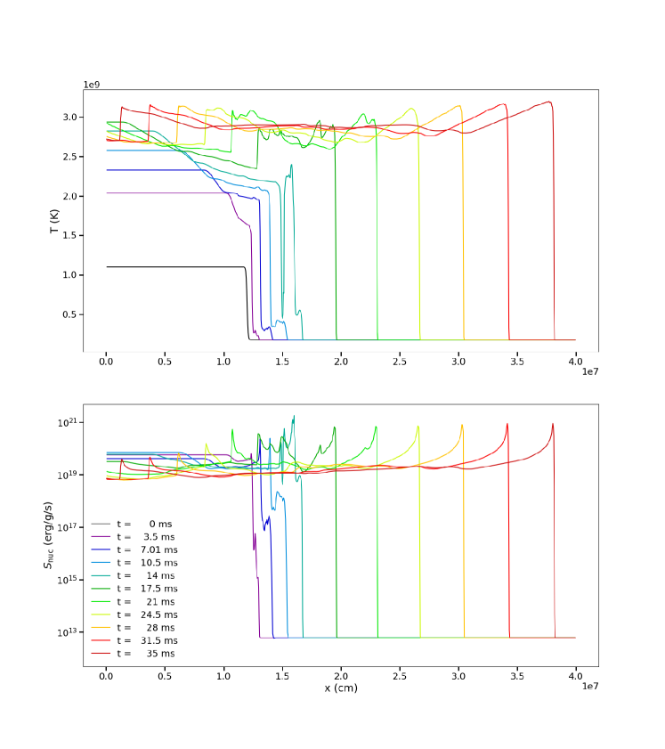
Figure 2 shows the time evolution of the temperature and specific nuclear energy generation rate using the He-C-Fe network. The peak temperature and specific energy generation rate reach $\sim 3\times 10^{9}$ K and $\sim 10^{21}~{}\mbox{erg}~{}\mbox{g}^{-1}~{}\mbox{s}^{-1}$, consistent with results of the shell-burning stage in the previous study [16].

Figure 3: Time evolution of the shock speed for different networks.

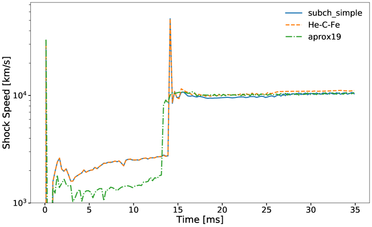
We now look at the effect of the network. Figure 3 shows the time evolution of the shock speed for our different networks. It is observed that all models reach a shock speed of $\sim 10^{4}$ $\mbox{km}\ \mbox{s}^{-1}$ after $\sim 15$ ms, while some noticeable differences for $t\lesssim 15$ ms. Specifically, He-C-Fe and subch_simple exhibit similar profiles, with roughly double the shock speed compared to aprox19 for $t\lesssim 15$ ms. This difference in shock speed is due to the missing ${}^{12}\mbox{C}(\mbox{p},\gamma){}^{13}\mbox{N}(\alpha,\mbox{p}){}^{16}\mbox{O}$ rate in aprox19, resulting in weaker initial carbon-burning [27, 28, 29]. A similar effect was seen with flames in XRBs in the study by [5].

(a) He-C-Fe. Both solid and dashed lines are used to better distinguishability.

(b) subch_simple

(c) aprox19

Figure 4: Time evolution of the total mass of ⁴He, ¹²C and iron-peak isotopes over time.

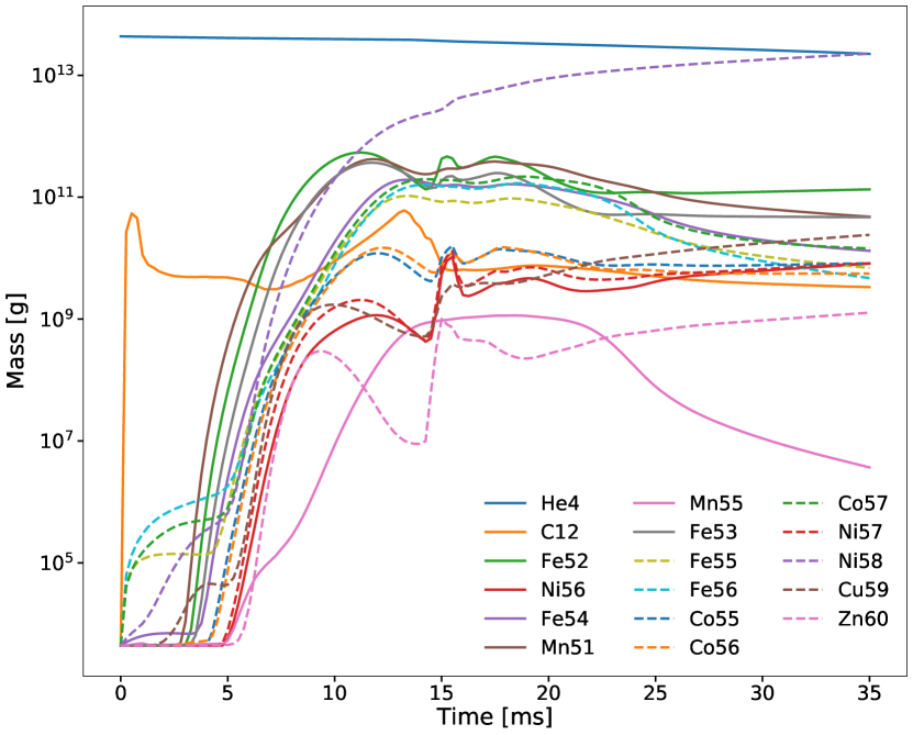
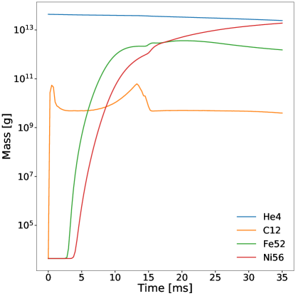
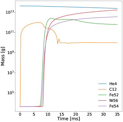
This carbon burning enhancement effect is evident when examining the total mass abundance of ¹²C in Figure 4, showing the time evolution of ⁴He, ¹²C, and iron-peak isotopes available in the network. The enhanced carbon burning path in both He-C-Fe and subch_simple leads to a greater ¹²C consumption rate, leading to a higher shock speed. After $\sim 15$ ms, the total mass of ¹²C stabilizes, reaching a steady speed for all three networks. In terms of iron-peak nucleosynthesis, both aprox19 and subch_simple indicate that ⁵⁶Ni is the primary product, whereas He-C-Fe predominantly yields ⁵⁸Ni. This insight is important for determining the correct mass abundance of ⁵⁶Ni following the explosion since the beta decay from ${}^{56}\mbox{Ni}\rightarrow{}^{56}\mbox{Co}\rightarrow{}^{56}\mbox{Fe}$ primarily shapes the observed SN Ia light curve.

Figure 5: Total number of CPU hours used for each network.

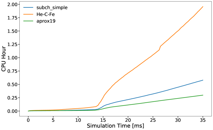
To demonstrate the computational cost associated with adding additional iron-peak isotopes, Figure 5 shows the CPU-hours used with each network. As expected, a larger network size corresponds to a higher CPU hour usage. Specifically, the CPU-hours used by He-C-Fe increased drastically after $15$ ms, coinciding with the establishment of the steady propagating detonation wave. In the end, He-C-Fe required nearly 4 times the CPU-hours compared to subch_simple, which has $\sim 1/3$ of the total number of rates in He-C-Fe. This result suggests the need for further simplification and optimization of the network before employing it in actual simulations such as a 2D sub-Chandrasekhar double detonation model.

4 Future Development

We’ve outlined the versatile approach for nuclear reaction sensitivity testing using pynucastro, Microphysics, and Castro. By leveraging pynucastro for network generation, Microphysics for network burning, and Castro for reaction-hydrodynamics coupling, we can effortlessly investigate any network of choice. Demonstrated through the 1D Detonation problem in Castro, we assess reaction network sensitivity and emulate shell-burning of the sub-Chandrasekhar double detonation model nucleosynthesis. In the future, this testing capability aims to identify an efficient network with sufficiently many iron-peak isotopes, similar to He-C-Fe, for studying nucleosynthesis in the actual sub-Chandrasekhar double detonation model.

Castro is open-source and freely available at http://github.com/AMReX-Astro/Castro. The work at Stony Brook was supported by DOE/Office of Nuclear Physics grant DE-FG02-87ER40317. This research was supported by the Exascale Computing Project (17-SC-20-SC), a collaborative effort of the U.S. Department of Energy Office of Science and the National Nuclear Security Administration. This research used resources of the National Energy Research Scientific Computing Center, a DOE Office of Science User Facility supported by the Office of Science of the U. S. Department of Energy under Contract No. DE-AC02-05CH11231. This research used resources of the Oak Ridge Leadership Computing Facility at the Oak Ridge National Laboratory, which is supported by the Office of Science of the U.S. Department of Energy under Contract No. DE-AC05-00OR22725, awarded through the DOE INCITE program. We thank NVIDIA Corporation for the donation of a Titan X and Titan V GPU through their academic grant program. This research has made use of NASA’s Astrophysics Data System Bibliographic Services.

References

- [1] Hillebrandt W and Niemeyer J C 2000 Annual Review of Astronomy and Astrophysics 38 191–230 (Preprint https://doi.org/10.1146/annurev.astro.38.1.191) URL https://doi.org/10.1146/annurev.astro.38.1.191
- [2] Maoz D, Mannucci F and Nelemans G 2014 Annual Review of Astronomy and Astrophysics 52 107–170 (Preprint https://doi.org/10.1146/annurev-astro-082812-141031) URL https://doi.org/10.1146/annurev-astro-082812-141031
- [3] Galloway D K and Keek L 2021 Timing Neutron Stars: Pulsations, Oscillations and Explosions (Astrophysics and Space Science Library vol 461) ed Belloni T M, Méndez M and Zhang C pp 209–262 (Preprint 1712.06227)
- [4] Woosley S E, Heger A, Cumming A, Hoffman R D, Pruet J, Rauscher T, Fisker J L, Schatz H, Brown B A and Wiescher M 2004 ASTROPHYS J SUPPL S 151 75–102 ISSN 0067-0049, 1538-4365 URL https://doi.org/10.1086/381533
- [5] Chen Z, Zingale M and Eiden K 2023 The Astrophysical Journal 955 128 URL https://dx.doi.org/10.3847/1538-4357/acec72
- [6] Zingale M, Malone C M, Nonaka A, Almgren A S and Bell J B 2015 ApJ 807 60 ISSN 1538-4357 (Preprint 1410.5796) URL https://doi.org/10.1088/0004-637x/807/1/60
- [7] Zingale M, Eiden K and Katz M 2023 ApJ 952 160 URL https://dx.doi.org/10.3847/1538-4357/ace04e
- [8] E Willcox D and Zingale M 2018 JOSS 3 588 ISSN 2475-9066 URL https://doi.org/10.21105/joss.00588
- [9] Clark A I S, Johnson E T, Chen Z, Eiden K, Willcox D E, Boyd B, Cao L, DeGrendele C J and Zingale M 2023 ApJ 947 65 URL https://dx.doi.org/10.3847/1538-4357/acbaff
- [10] AMReX-Astro Microphysics Development Team, Bishop A, Fields C E, Chen Z, Harpole A, Jacobs A M, Johnson E, Katz M, Li X, Malone C, Timmes F, Willcox D and Zingale M 2023 Amrex-astro/microphysics: Release 23.08 URL https://doi.org/10.5281/zenodo.8206742
- [11] Almgren A S, Beckner V E, Bell J B, Day M S, Howell L H, Joggerst C C, Lijewski M J, Nonaka A, Singer M and Zingale M 2010 ApJ 715 1221–1238 ISSN 0004-637X, 1538-4357 (Preprint 1005.0114) URL https://doi.org/10.1088/0004-637x/715/2/1221
- [12] Almgren A, Sazo M B, Bell J, Harpole A, Katz M, Sexton J, Willcox D, Zhang W and Zingale M 2020 JOSS 5 2513 URL https://doi.org/10.21105/joss.02513
- [13] Cyburt R H, Amthor A M, Ferguson R, Meisel Z, Smith K, Warren S, Heger A, Hoffman R D, Rauscher T, Sakharuk A, Schatz H, Thielemann F K and Wiescher M 2010 ApJS 189 240–252 ISSN 0067-0049, 1538-4365 URL https://doi.org/10.1088/0067-0049/189/1/240
- [14] Suzuki T, Toki H and Nomoto K 2016 ApJ 817 163 URL https://dx.doi.org/10.3847/0004-637X/817/2/163
- [15] LANGANKE K and MARTÍNEZ-PINEDO G 2001 Atomic Data and Nuclear Data Tables 79 1–46 ISSN 0092-640X URL https://www.sciencedirect.com/science/article/pii/S0092640X01908654
- [16] Zingale M, Chen Z, Rasmussen M, Polin A, Katz M, Clark A S and Johnson E T 2023 Sensitivity of simulations of double detonation type ia supernova to integration methodology (Preprint 2309.01802)
- [17] Nomoto K, Iwamoto K, Nakasato N, Thielemann F K, Brachwitz F, Tsujimoto T, Kubo Y and Kishimoto N 1997 Nucl. Phys. A 621 467–476 (Preprint astro-ph/9706025)
- [18] Parikh A, José J, Sala G and Iliadis C 2013 Prog. Part. Nucl. Phys. 69 225–253 ISSN 0146-6410 (Preprint 1211.5900) URL https://doi.org/10.1016/j.ppnp.2012.11.002
- [19] Bravo, E 2019 A&A 624 A139 URL https://doi.org/10.1051/0004-6361/201935095
- [20] Lach, F, Röpke, F K, Seitenzahl, I R, Coté, B, Gronow, S and Ruiter, A J 2020 A&A 644 A118 URL https://doi.org/10.1051/0004-6361/202038721
- [21] Zingale M, Katz M P, Nonaka A and Rasmussen M 2022 ApJ 936 6 URL https://dx.doi.org/10.3847/1538-4357/ac8478
- [22] Timmes F X 2019 aprox13 network URL https://cococubed.com/code_pages/burn_helium.shtml
- [23] Timmes F X and Swesty F D 2000 ApJS 126 501–516 ISSN 0067-0049, 1538-4365 URL https://doi.org/10.1086/313304
- [24] Brown P N, Byrne G D and Hindmarsh A C 1989 SIAM J. Sci. and Stat. Comput. 10 1038–1051 ISSN 0196-5204, 2168-3417 URL https://doi.org/10.1137/0910062
- [25] Fink M, Hillebrandt W and Röpke F K 2007 A&A 476 1133–1143 (Preprint 0710.5486)
- [26] Weaver T A, Zimmerman G B and Woosley S E 1978 ApJ 225 1021 ISSN 0004-637X, 1538-4357 URL https://doi.org/10.1086/156569
- [27] Weinberg N N, Bildsten L and Schatz H 2006 ApJ 639 1018–1032 (Preprint astro-ph/0511247)
- [28] Fisker J L, Schatz H and Thielemann F 2008 ApJS 174 261–276 ISSN 0067-0049, 1538-4365 URL https://doi.org/10.1086/521104
- [29] Shen K J and Bildsten L 2009 ApJ 699 1365–1373 URL https://doi.org/10.1088%2F0004-637x%2F699%2F2%2F1365