Predicting the morphology of multiphase biomolecular condensates from protein interaction networks

Abstract

Phase-separated biomolecular condensates containing proteins and RNAs can assemble into higher-order structures by forming thermodynamically stable interfaces between immiscible phases. Using a minimal model of a protein/RNA interaction network, we demonstrate how a “shared” protein species that partitions into both phases of a multiphase condensate can function as a tunable surfactant that modulates the interfacial properties. We use Monte Carlo simulations and free-energy calculations to identify conditions under which a low concentration of this shared species is sufficient to trigger a wetting transition. We also describe a numerical approach based on classical density functional theory to predict concentration profiles and surface tensions directly from the model protein/RNA interaction network. Finally, we show that the wetting phase diagrams that emerge from our calculations can be understood in terms of a simple model of selective adsorption to a fluctuating interface. Our work shows how a low-concentration protein species might function as a biological switch for regulating multiphase condensate morphologies.

I Introduction

Intracellular biomolecular mixtures can spatially organize into complex, self-assembled compartments via phase separation [1, 2, 3]. Such structures are referred to as biomolecular condensates, since they form by spontaneously condensing biomolecular components, such as proteins and RNAs, into liquid-like compartments that are not enclosed by a membrane [4]. In many instances, condensates have been observed to assemble further into higher-order multiphasic structures, in which multiple immiscible condensates form stable shared interfaces [5, 6, 7]. Common multiphase morphologies include “core–shell” architectures, in which one condensate is completely surrounded by a second condensate, and “docked” architectures, in which condensed droplets attach to the surface of another condensate [8]. The morphologies of many multiphase condensates appear to be related to their biological functions, such as the sequential processing of rRNA transcripts during ribogenesis within core–shell nucleoli [9], and the sharing of various biomolecular components between docked stress granule and P-body condensates that are involved in regulating mRNA metabolism and translation [7, 10, 11]. It is therefore important to understand how the morphologies of multiphase condensates are controlled at a molecular level.

The formation of biomolecular condensates is widely considered to be a consequence of near-equilibrium, thermodynamically driven phase separation [12, 13, 14]. Within this thermodynamic framework, a multicomponent system evolves to minimize its overall free energy by phase-separating and adjusting the contact areas between different phases. The equilibrium morphology of a multiphase system is thus governed by the relationships among surface tensions between pairs of phases and the volume fractions of the phases [15, 16]. Recent theoretical studies have demonstrated that surface tensions in multicomponent mixtures, and consequently multiphase morphologies, can be controlled by changing either the effective pairwise interactions between the biomolecular components [16] or the stoichiometry of multicomponent condensates that are stabilized by heterotypic interactions [17]. However, changing condensate morphologies via these mechanisms entails substantial changes to the state of the system, since the molecular properties and/or concentrations of the components that comprise the bulk of the phase-separated condensates must be altered.

By contrast, surface tensions can be tuned by making comparably small perturbations to molecular components that adsorb to condensate interfaces [18, 19, 20]. In principle, tuning the concentrations and affinities of surfactant-like components can control multiphase condensate morphologies with minimal changes to the state of an intracellular mixture. A key example is provided by a recent study [21] of stress granules (SGs) and P-bodies (PBs), which assemble into a docked multiphase architecture under stressed conditions in human cells [11]. Importantly, this study suggested that small changes to the concentrations of specific proteins—in particular, those with affinities for proteins in each of the coexisting SG and PB phases—can trigger a wetting transition between docked and dispersed condensates [21]. Although the localization of these particular proteins to the SG/PB interface has not been confirmed experimentally, this example suggests that molecular components with affinities for the constituents of multiple distinct condensates can alter the morphologies of multiphase condensates, even at low concentrations.

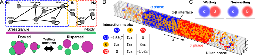
Figure 1: Minimal model of multiphase condensates. (A) Schematic of the protein/RNA interaction network that governs stress granule (SG)/P-body (PB) multiphase condensates [21]. Top: Nodes indicate protein/RNA species, while edges indicate either homotypic interactions (i.e., self associations) or heterotypic interactions (i.e., associations between different species). We coarse-grain the network into N1, B, and N2 species. The approximate partitioning of various species into the SG/PB condensates is suggested by the color bar below. Bottom: SG/PB condensates form either docked or dispersed morphologies, depending on the interactions specified by the network and the concentrations of the protein/RNA species. (B) A typical configuration of the coarse-grained direct-coexistence simulations showing the $\alpha$ and $\beta$ condensed phases, composed primarily of the N1 (blue) and N2 (red) species, respectively, and a coexisting dilute phase. The low-concentration B species (gold) is dispersed throughout the simulation box. The interaction matrix, $\bm{\epsilon}$, for the nearest-neighbor intermolecular interactions is shown in the inset. (C) The $\alpha$ and $\beta$ phases adopt either a wetting (left) or non-wetting (right) configuration depending on the relationship between the $\alpha$–$\beta$, $\alpha$–dilute, and $\beta$–dilute surface tensions.

In this article, we investigate this proposed mechanism for switching between morphologies of multiphase condensates. Specifically, we use a minimal model of a multicomponent mixture to derive design rules for controlling wetting transitions via low-concentration “programmable surfactant” proteins, which interact selectively with the constituents of two immiscible condensates. We first introduce a simulation approach for computing the wetting transition between docked and dispersed morphologies. We then develop a complementary theoretical approach based on classical density functional theory, which reproduces our simulation results semi-quantitatively. Both approaches predict that relatively low concentrations of surfactant-like proteins can trigger a wetting transition between docked and dispersed morphologies under specific conditions. Finally, we describe a qualitative theory that predicts the key features of this wetting transition and establishes rational design rules for understanding the behavior of programmable surfactants in multicomponent biomolecular mixtures. Taken together, our results show how programmable surfactants can act as low-concentration molecular switches for regulating biological processes by controlling the morphologies of multiphase condensates.

II Minimal model of a programmable surfactant

Our model is motivated by the multicomponent SG/PB system studied in Ref. [21]. At a molecular level, the formation of the immiscible SG and PB condensates is dictated by the interactions among the constituent protein and mRNA components. In this system, the relevant intermolecular interactions can be described by a protein/RNA interaction network (Fig. 1A), in which nodes represent proteins, protein complexes, or RNA, and edges indicate attractive interactions between species.

To reduce the complexity, we coarse-grain the endogenous SG/PB protein/RNA interaction network to three explicit molecular components based on the organization of the network. We refer to these coarse-grained species as “Node 1” (N1), “Bridge” (B), and “Node 2” (N2) throughout this work. N1 and N2 are the majority components of the immiscible $\alpha$ and $\beta$ condensed phases, respectively, that form as a result of attractive homotypic interactions (Fig. 1B). The heterotypic interactions between the N1 and N2 species are set to zero to ensure immiscibility of the $\alpha$ and $\beta$ phases. By contrast, B represents a “shared” species that interacts with the majority components of the $\alpha$ and $\beta$ phases via attractive heterotypic interactions. The homotypic and heterotypic interactions among these species are summarized in a pairwise interaction matrix $\bm{\epsilon}$ [22] (Fig. 1B). The $\alpha$ and $\beta$ phases coexist with a dilute phase (D), which represents the cytosol in our implicit-solvent model.

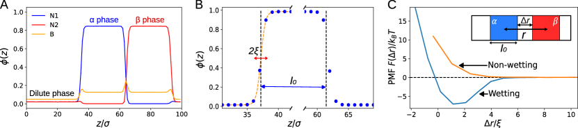
Figure 2: Characterizing interfaces using Monte Carlo simulations and umbrella sampling. (A) Trajectory-averaged molecular volume-fraction profiles under conditions where a wetting interface forms between two condensed phases. Enrichment of B molecules is observed at the $\alpha$–$\beta$ and condensed–dilute interfaces. (B) Definitions of the characteristic interfacial width parameter, $\xi$, and the width of a single condensed phase, $l_{0}$. (C) The potential of mean force (PMF) as a function of the dimensionless distance parameter $\Delta r/\xi$ between the Gibbs dividing surfaces of the $\alpha$ and $\beta$ phases (see inset). Example PMFs are shown for typical wetting (orange) and non-wetting (blue) scenarios. Statistical errors are smaller than the line width.

For simplicity, we consider a three-dimensional lattice-gas model in which the N1, N2, and B species occupy individual lattice sites on a cubic lattice with lattice constant $\sigma$. Each molecule interacts with its six nearest neighbors according to the interaction matrix, $\bm{\epsilon}$. Vacant lattice sites represent the inert solvent. Since we are interested in investigating how the B species controls the condensate interfaces as opposed to the properties of the bulk phases, we choose to keep the homotypic N1 and N2 interactions constant in this work. We fix these interaction strengths to be $1.5k_{\text{B}}T$ per bond, which is stronger than the critical binding strength $\sim 0.89\,k_{\text{B}}T$ of the cubic lattice gas model [23]. This choice guarantees stable $\alpha$ and $\beta$ condensed phases. Furthermore, under these conditions, the N1 and N2 concentrations primarily affect the volume fractions of the coexisting $\alpha$, $\beta$, and dilute phases and have negligible effects on the compositions of the condensed phases. The interaction energies describing heterotypic N1–B and N2–B interactions, $\epsilon_{\text{NB}}$, and homotypic B–B interactions, $\epsilon_{\text{BB}}$, are left as free parameters. This model is most appropriate for describing highly multivalent protein and RNA species, in which the net interactions between pairs of molecules can be approximated via isotropic pair interactions [22]. In particular, this minimal model is a reasonable approximation of complex protein/RNA interactions when the discrete contributions from associating protein domains and RNA sequence motifs are relatively weak compared to the thermal energy [22].

III Computing wetting transitions via molecular simulation

In this section, we introduce a Monte Carlo technique for computing the wetting transition between docked and dispersed morphologies of a multiphase condensate (Fig. 1C). We first describe the set-up of direct-coexistence simulations [24] in the canonical ensemble, from which we determine the potential of mean force (PMF) between a pair of condensed phases. We then show how the properties of these PMFs can be related to the equilibrium morphology of a macroscopic multiphase system in the thermodynamic limit.

III.1 Direct-coexistence Monte Carlo simulations

We implement direct-coexistence Monte Carlo simulations in the slab geometry [24], using a $100\times 8\times 8$ lattice with periodic boundary conditions. This geometry results in approximately planar interfaces between coexisting phases (Fig. 1B). We fix the volume fractions of the N1 and N2 species to be $\phi_{\text{N1}}=\phi_{\text{N2}}=0.25$, such that the condensed phases occupy approximately half the total volume. Simulations are carried out using the Metropolis Monte Carlo algorithm [25], where we attempt to exchange the positions of molecules of different types at each Monte Carlo (MC) move.

The typical behavior of the multiphase system in this slab geometry can be understood by examining molecular volume-fraction profiles, $\vec{\phi}(z)$, as a function of the $z$ coordinate along the long dimension of the simulation box. To this end, we compute $\vec{\phi}(z)$ every 10 MC sweeps and average 20,000 such profiles; we then report the mean profile averaged over 10 independent, equilibrated trajectories (Fig. 2A). The interface between a condensed phase and the dilute phase is well described by a hyperbolic tangent function [26], $\phi_{\text{N1}}(z)={(1/2)(\phi_{\text{N1}}^{(\alpha)}+\phi_{\text{N1}}^{(\text{D})})}+{(1/2)(\phi_{\text{N1}}^{(\alpha)}-\phi_{\text{N1}}^{(\text{D})})\text{tanh}[(z-z_{0})/\xi)]}$, where $\phi_{\text{N1}}^{(\alpha)}$ and $\phi_{\text{N1}}^{(\text{D})}$ are the volume fractions occupied by the molecular species N1 in the bulk $\alpha$ and dilute phases, respectively (Fig. 2B). This expression is used to define the interfacial width, which is equal to $2\xi$. We also define the width of the $\alpha$ condensed phase, $l_{0}$, based on the distance between the left and right Gibbs dividing surfaces, where $\phi_{\text{N1}}(z)=(\phi_{\text{N1}}^{(\alpha)}+\phi_{\text{N1}}^{(\text{D})})/2$. These parameters are used in the interpretation of the PMF calculations described next.

III.2 Potential of mean force (PMF) calculations

To efficiently sample both wetting and non-wetting configurations, we perform umbrella sampling [27] by applying a harmonic biasing potential to the center-of-mass (COM) distance between the $\alpha$ and $\beta$ condensates. We first define the $\alpha$ and $\beta$-phase regions, $S_{\alpha/\beta}$, as the cross-sections along the $z$ axis of the simulation box with N1 or N2 volume fractions greater than $\phi^{*}$: $S_{\alpha/\beta}\equiv\{z\ |\ \phi_{\text{N1}/\text{N2}}(z)>\phi^{*}\}$. We find that using a threshold of $\phi^{*}=0.56$ reduces the effects of density fluctuations near the interfaces and thus improves the efficiency of our calculations; however, this choice has no significant effect on the results, as long as $\phi^{*}$ is situated between the molecular volume fractions of the bulk condensed and dilute phases. We then compute the COM distance, $r$, based on the center of mass of the N1 or N2 molecules within the $\alpha$ or $\beta$ phases, respectively. The COM distance is therefore $r\equiv\langle z\rangle^{(\beta)}-\langle z\rangle^{(\alpha)}$, where $\langle z\rangle^{(\alpha/\beta)}\equiv\int_{z\in S_{\alpha/\beta}}z\,dz/\int_{z\in S_{\alpha/\beta}}dz$, and we use the minimum-image convention to define distances given the periodic boundary conditions.

Our aim is to compute the PMF

$$F(r)\equiv-k_{\text{B}}T\ln\frac{p(r)}{p(r_{\text{ref}})},$$ (1)

where $p(r)$ is the probability of finding the $\alpha$ and $\beta$ condensed phases separated by a COM distance equal to $r$. We choose a reference point for the PMF calculations where the interactions between the droplets are expected to be negligible ($r_{\text{ref}}=35\sigma$ in our simulation geometry). Following the canonical umbrella sampling approach [27], we apply a harmonic biasing potential, $(k_{i}/2)(r-r_{0,i})^{2}$, to constrain the COM distance near a target distance $r_{0,i}$. Independent simulations, indexed by $i=1,\ldots,M$, are used to sample COM distances near target values in the range $25\sigma\leq r_{0,i}\leq 35\sigma$ at intervals of one $\sigma$. The spring constants $\{k_{i}\}$ are chosen to ensure that the probability distributions, $p_{i}(r)$, sampled from simulations at adjacent target distances overlap [28]. In production simulations, we calculate the COM distance every 10 MC sweeps and record 20,000 samples for every target distance $\{r_{0,i}\}$. Finally, we utilize the multistate Bennett acceptance ratio (MBAR) method [29] to combine samples from the $M$ independent biased simulations and to obtain the unbiased PMF given by Eq. (1). Example PMF calculations are shown in Fig. 2C.

III.3 Morphology predictions using the PMF

The PMF defined via Eq. (1) reflects the propensity for the $\alpha$ and $\beta$ condensed phases to assemble into a docked configuration, since the minimum value of the PMF corresponds to the equilibrium distance between the Gibbs dividing surfaces. To assist in interpreting the PMF calculations, we characterize the distance between the $\alpha$ and $\beta$-phase interfaces by defining a dimensionless distance parameter $\Delta r/\xi\equiv(r-l_{0})/\xi$ (see inset of Fig. 2C). $\Delta r/\xi$ is equal to zero when the Gibbs dividing surfaces of the two condensed phases are in direct contact, whereas $\Delta r/\xi\gg 1$ indicates that the distance between the condensed-phase interfaces is large compared to the typical interfacial fluctuations.

Two representative PMFs for wetting and non-wetting scenarios are shown in Fig. 2C. In the non-wetting case, the PMF is non-negative, indicating a net repulsion between the $\alpha$ and $\beta$ phases. We find that the PMF begins to increase as $\Delta r/\xi$ decreases below $\sim 4$, suggesting that the fluctuating interfaces interact well before the Gibbs dividing surfaces come into contact. By contrast, the PMF has a clear minimum in the wetting case. The negative values of the PMF at COM distances in the range $0\lesssim\Delta r/\xi\lesssim 4$ indicate a net attraction between the $\alpha$ and $\beta$ condensed phases that also occurs over a length scale comparable to that of the interfacial fluctuations. In what follows, we show that the condensate morphology in the thermodynamic limit can be predicted on the basis of PMF calculations obtained from these finite-size simulations.

Within a finite simulation box, the probability of distribution of the $\alpha$–$\beta$ COM distance is related to the PMF via $p(r)\propto e^{-F(r)/k_{\text{B}}T}=e^{-Af(r)/k_{\text{B}}T}$, where $A$ is the cross-sectional area of the simulation box and $f(r)$ is the PMF per unit area. Consistent with this expectation, we indeed find that the PMF profiles scale with $A$ in our simulations in both wetting and non-wetting cases (Fig. 3). These results indicate that the PMFs capture extensive properties of the condensed-phase interfaces in our model and are not significantly influenced by the dimensions of the simulation box. Next, we define a contact distance $r_{\text{c}}=l_{0}+\lambda$ beyond which we consider the condensates to be in a non-wetting configuration, such that $F(r_{\text{c}})\simeq 0$. Here $l_{0}$ depends on the width of the condensed phase (see, e.g., Fig. 2B) while $\lambda$ is a constant. The probability of finding the $\alpha$ and $\beta$ condensed phases in a wetting configuration in a simulation box of length $L$ can then be written as

$$p_{\text{w}}=\frac{Z_{\text{w}}}{Z_{\text{w}}+Z_{\text{nw}}},$$ (2)

where $Z_{\text{w}}\equiv\int^{r_{\text{c}}}_{0}e^{-Af(r)/k_{\text{B}}T}dr$ and $Z_{\text{nw}}=L/2-r_{\text{c}}$ are the partition functions associated with the wetting and non-wetting macrostates, respectively.

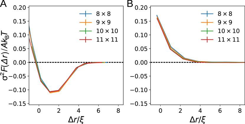
Figure 3: Finite-size scaling of the PMFs. PMFs collapse onto a single curve when scaled by the cross-sectional area, $A=\sigma^{2}l^{2}$, in both (A) wetting ($\epsilon_{\text{NB}}=-1k_{\text{B}}T$, $\epsilon_{\text{BB}}=0$, $\phi_{\text{B}}=0.1$) and (B) non-wetting ($\phi_{\text{B}}=0$) examples. The cross-sectional dimensions of the lattice, $l\times l$, are indicated for each curve in units of $\sigma$. Statistical errors are smaller than the line width.

Now we consider changing the geometry of the simulation box while keeping the concentrations of all molecular species unchanged. As a result, the volume associated with each condensed phase, $l_{0}A$, scales with the system size, while the volume fractions and compositions of the condensed phases remain constant. Since $Z_{\text{w}}$ depends on the cross-sectional area $A$ and $Z_{\text{nw}}$ depends on the box length $L$, the wetting probability depends on both $A$ and $L$ in a finite-size simulation box. The $L$-dependence indicates that configurational entropy plays a role in determining $p_{\text{w}}$ in a finite-size system, implying that the probability of forming a wetting interface tends to zero if the simulation box is elongated with the cross-sectional area $A$ held constant. However, in the thermodynamic limit, both $A$ and $L$ are taken to infinity with the ratio $A/L$ held constant. The wetting probability then tends to either one or zero, depending on whether the minimum of the PMF is less than zero. If the PMF minimum is negative, then $Z_{\text{w}}$ scales exponentially with $A$ while $Z_{\text{nw}}$ scales with $A^{1/2}$; in this case, $p_{\text{w}}=1$ according to Eq. (2). By contrast, if the minimum value of $F(r)$ is non-negative, then $Z_{\text{w}}$ decreases with $A$, and $p_{\text{w}}=0$. Finally, by comparing our condition for a docked configuration in the thermodynamic limit to the macroscopic condition for partial wetting [30], we obtain a relationship between the PMF minimum, $F(r_{\text{eq}})$, and the surface tensions between the condensed phases, $\gamma_{\alpha\beta}$, and between the dilute and condensed phases, $\gamma_{\alpha\text{D}}$,

$$F(r_{\text{eq}})=A(\gamma_{\alpha\beta}-2\gamma_{\alpha\text{D}}).$$ (3)

Thus, the multiphase morphology is determined solely by the PMF, or equivalently by the surface-tension difference $\gamma_{\alpha\beta}-2\gamma_{\alpha\text{D}}$, in the thermodynamic limit.

These arguments are easily extended to describe the morphology of spherical multiphase condensates. The finite-size wetting probability, Eq. (2), is now determined from the partition functions $Z_{\text{w}}=4\pi\int^{r_{\text{c}}}_{0}e^{-A(r)f(r)/k_{\text{B}}T}r^{2}dr$ and $Z_{\text{nw}}=V-(4\pi/3)r_{\text{c}}^{3}$, where the interfacial area, $A(r)$, depends on the COM distance, $r$. The non-wetting partition function, $Z_{\text{nw}}$, represents the free volume available to a non-wetted condensate, and $V$ is the total volume of the system. In the thermodynamic limit, an analogous scaling argument implies that the wetting behavior again depends solely on the surface-tension difference, which is related to the PMF minimum via Eq. (3). When $\gamma_{\alpha\beta}-2\gamma_{\alpha\text{D}}<0$, the docked condensates take the shape of spherical caps [31], forming a circular interface with contact angle $\theta=\arccos(\gamma_{\alpha\beta}/2\gamma_{\alpha\text{D}})$; otherwise, spherical $\alpha$ and $\beta$ condensates do not form a stable shared interface in the thermodynamic limit.

IV Predicting multiphase morphology with classical density functional theory

In this section, we develop a complementary approach for predicting multiphase condensate morphologies using the framework of classical density functional theory (CDFT). This theoretical framework utilizes a “square-gradient” free-energy functional [26], which yields the Cahn–Hilliard (CH) formula [32] for the surface tension of a binary mixture. However, a straightforward generalization [15, 16, 21] of the CH formula to our multicomponent model predicts non-wetting behavior for a wide range of conditions, which is at odds with our simulation results. To this end, we show how improved predictions for the equilibrium molecular volume-fraction profiles and surface tensions can be obtained within the CDFT framework. We then discuss how our approach differs from the CH formula in multicomponent systems.

IV.1 Phase behavior of the regular solution model

Assuming a regular solution model [33], the Helmholtz free-energy density, $f_{0}$, of the multicomponent lattice gas can be written as

$$\frac{f_{0}\sigma^{3}}{k_{\text{B}}T}=\sum_{i}\phi_{i}\ln\phi_{i}+\frac{1}{2}\sum_{i,j}\phi_{i}\chi_{ij}\phi_{j},$$ (4)

where the sums run over all $N$ molecular components as well as the implicit solvent. The molecular volume fractions are constrained by an incompressibility condition, $\sum^{N}_{i=0}\phi_{i}=1$, where $\phi_{0}$ represents the volume fraction of the solvent. The interaction matrix $\chi_{ij}$ is related to the nearest-neighbor interaction energy, $\epsilon_{ij}$, by $\chi_{ij}\equiv(z/2k_{\text{B}}T)(2\epsilon_{ij}-\epsilon_{ii}-\epsilon_{jj})$, where the lattice coordination number is $z=6$.

We compute the bulk phase behavior of this model by satisfying the equal chemical potential and equal pressure conditions in all coexisting phases [34]. We also enforce a mass conservation constraint on the total molecular volume fraction of each species in the system. Details of these calculations and their numerical implementation are provided in Appendix A. For the interaction matrix shown in Fig. 1B, Eq. (4) predicts three coexisting phases, $\alpha$, $\beta$, and D, when $\phi_{\text{B}}$ is small, in agreement with our Monte Carlo simulations. In general, the mean-field regular solution model provides an adequate description of the condensed phases and their interfaces under these conditions, which are chosen to be sufficiently far from the critical points of the condensed phases.

IV.2 Classical density function theory (CDFT)

In the grand canonical ensemble, we express the grand-potential functional in terms of the square-gradient approximation [26],

$$\Omega[\{\phi_{i}\}]=A\!\!\int\!\left[\omega_{0}[\vec{\phi}(z)]+\frac{1}{2}\sum_{i,j}\phi^{\prime}_{i}(z)m_{ij}\phi^{\prime}_{j}(z)\right]\!dz,$$ (5)

assuming planar interfaces as in our simulations. $\Omega$ is a functional of the molecular volume fractions, $\{\phi_{i}\}$, in a system at fixed chemical potentials, $\{\mu_{i}\}$. For interfacial property calculations, the chemical potentials are determined from the aforementioned coexistence conditions, such that the bulk phases far from an interface are in coexistence. The first term in the integrand of Eq. (5) is the local grand-potential density, $\omega_{0}\equiv f_{0}-\sum_{i}\mu_{i}\phi_{i}$, while the second term represents the excess grand potential due to an inhomogeneity, such as an interface between coexisting phases. Although this square-gradient approximation is most applicable to inhomogeneities that vary slowly in space due to the absence of higher-order derivatives [26], we find that Eq. (5) can yield remarkably accurate predictions with respect to our simulations, as we show below.

We approximate the coefficients of the square-gradient term, $\bm{m}=\{m_{ij}\}$, by again assuming that the inhomogeneity is small in amplitude and varies slowly in space. For the free-energy density given in Eq. (4), these conditions imply that

$$m_{ij}=-\sigma^{-1}\epsilon_{ij}$$ (6)

is a constant, concentration-independent matrix [26, 32]. However, in our multicomponent model, this coefficient matrix may not be positive-semidefinite, as required by the long-wavelength assumption underlying the square-gradient approximation. If the coefficient matrix instead has negative eigenvalues, then large-amplitude inhomogeneities act to decrease the grand potential, leading to unphysical negative surface tensions and numerical instabilities. Qualitatively, this scenario tends to occur when heterotypic interactions out-compete one or more homotypic interactions. We propose that the square-gradient approximation can nonetheless be applied to multicomponent solutions in such scenarios by regularizing the $\bm{m}$-matrix. We therefore perform an eigenvalue decomposition of Eq. (6), replace the negative eigenvalues (if there are any) with zeroes, and reconstruct the regularized low-rank [35] $\bm{m}$-matrix for use in Eq. (5). We find that this approach leads to semi-quantitative predictions for the molecular volume-fraction profiles across a wide variety of conditions.

Finally, the equilibrium interfaces between coexisting phases are determined by minimizing the grand-potential functional,

$$\frac{\delta\Omega[\{\phi_{i}\}]}{\delta\phi_{i}}=0,$$ (7)

which yields the equilibrium molecular volume-fraction profiles, $\vec{\phi}_{\text{eq}}(z)$. We then calculate the excess free-energy profile, $\Delta\omega(z)$, in the vicinity of an interface between bulk phases,

$$\Delta\omega(z)=\omega_{0}[\vec{\phi}_{\text{eq}}(z)]-\omega_{0}^{(\text{D})}+\frac{1}{2}\sum_{i,j}\phi^{\prime}_{\text{eq},i}(z)m_{ij}\phi^{\prime}_{\text{eq},j}(z),$$ (8)

where $\omega^{(\text{D})}$ is the grand potential of the bulk dilute phase. The associated surface tension,

$$\gamma=\int\Delta\omega(z)dz,$$ (9)

is obtained by integrating the excess free-energy profile across the interface. The Euler–Lagrange equation specified by Eq. (7) must be solved numerically for our multicomponent model. In practice, this can be achieved by minimizing $\Omega[\{\phi_{i}(z)\}]$ via gradient descent. Details regarding our implementation of this numerical scheme, as well as criteria for assessing convergence, are presented in Appendix B.

IV.3 Comparison with the Cahn–Hilliard formula

We emphasize that the numerical results that we obtain by solving Eq. (7) differ qualitatively from a multicomponent generalization [15, 16, 21] of the Cahn–Hilliard (CH) formula for the surface tension [32]. Following the CH approach for a binary mixture [32], we can integrate the Euler–Lagrange equation, Eq. (7), to obtain

$$\omega_{0}[\vec{\phi}_{\text{eq}}(z)]-\omega_{0}^{(\text{D})}=\frac{1}{2}\sum_{i,j}\phi^{\prime}_{\text{eq},i}(z)m_{ij}\phi^{\prime}_{\text{eq},j}(z),$$ (10)

which relates the bulk and square-gradient contributions to the excess free energy, Eq. (8), of the equilibrium interface. However, in a multicomponent system, the path taken through concentration space between a pair of coexisting bulk phases 1 and 2 must also be specified. This path can be described parametrically by $\vec{\phi}(\eta)$, with $0\leq\eta(z)\leq 1$, $\lim_{z\rightarrow-\infty}\eta(z)=0$, and $\lim_{z\rightarrow\infty}\eta(z)=1$. If $\vec{\phi}(\eta)$ is assumed to be a linear path in concentration space, such that $\vec{\phi}(\eta)=(1-\eta)\vec{\phi}^{(1)}+\eta\vec{\phi}^{(2)}$, then we recover the multicomponent generalization of the CH formula [15, 16, 21],

$$\gamma_{12}=\sqrt{2(\phi^{(2)}_{i}-\phi^{(1)}_{i})m_{ij}(\phi^{(2)}_{j}-\phi^{(1)}_{j})}\int^{1}_{0}[\Delta\omega_{0}(\eta)]^{1/2}d\eta,$$ (11)

where $\Delta\omega_{0}(\eta)\equiv\omega_{0}(\vec{\phi}(\eta))-\omega_{0}^{(\text{D})}$. Importantly, this linear-path assumption implies that if the B component in our model is not enriched in either the $\alpha$ or the $\beta$ condensed phases, then it cannot be enriched at the $\alpha$–$\beta$ interface. As we will show below, this prediction is inconsistent with our simulation results, in which the B component tends to stabilize the $\alpha$–$\beta$ interface in wetting scenarios. For the same reason, Eq. (11) fails to predict wetting configurations for all conditions that we consider in this work.

The approximation leading to Eq. (11) is equivalent to minimizing only the square-gradient term of $\Omega$, and then applying the equilibrium relation between the bulk and square-gradient contributions to the excess free energy given in Eq. (10). A natural alternative approximation is to minimize only the bulk contribution to the excess free energy. This approximation leads to a minimum-free-energy path (MFEP) assumption for $\vec{\phi}(\eta)$. Specifically, the MFEP is the path in concentration space that minimizes the integral $\int_{0}^{1}\Delta\omega_{0}(\eta)\,d\eta$ and thus goes through a saddle point on the grand-potential landscape between the bulk-phase concentrations $\phi^{(1)}$ and $\phi^{(2)}$. By contrast with the linear-path assumption, the MFEP tends to predict enrichment of the B component at the interface whenever $\epsilon_{\text{NB}}<0$. The MFEP can be determined numerically from the bulk excess free energy landscape $\Delta\omega_{0}(\vec{\phi})\equiv\omega_{0}(\vec{\phi})-\omega_{0}^{(\text{D})}$ using the zero-temperature string method [36] (see Appendix C).

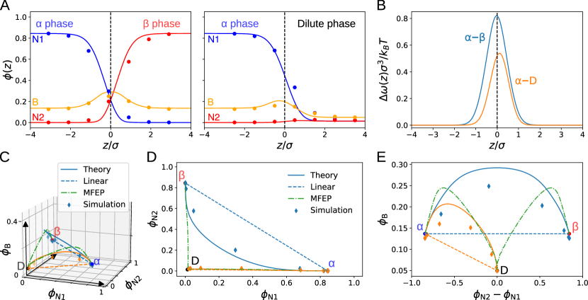
Figure 4: Enrichment of the programmable surfactant at condensate interfaces. (A) CDFT predictions (solid lines) closely agree with simulation measurements (points) of the equilibrium concentration profiles at $\alpha$–$\beta$ (left) and $\alpha$–dilute (right) interfaces. Vertical dashed lines indicate the Gibbs dividing surfaces. Results are shown for a typical wetting case ($\epsilon_{\text{NB}}=-1\,k_{\text{B}}T$, $\epsilon_{\text{BB}}=0$, $\phi_{\text{B}}=0.1$). (B) Excess free-energy profiles corresponding to the CDFT profiles shown in A. (C–E) Concentration profiles across the interfaces trace out paths in the three-dimensional (N1, N2, B) concentration space. Comparisons are shown between the simulation results (points), the full CDFT theory (solid lines), the linear-path approximation (dashed lines), and the minimum-free-energy-path (MFEP) approximation (dash-dotted lines) for the cases shown in A. Simulation statistical errors are comparable to the symbol size.

In general, we find that the optimal path, $\vec{\phi}_{\text{eq}}(\eta)$, is intermediate between the linear path and the MFEP. This optimal path therefore results from a competition between the bulk and square-gradient contributions to the grand-potential functional in our multicomponent model, which is not a consideration in the simpler case of a binary mixture. For this reason, the optimal path is sensitive to the $\bm{m}$-matrix, making regularization of the $\bm{m}$-matrix an essential step. Remarkably, we find that computing optimal paths via direct evaluation of Eq. (7) predicts both wetting and non-wetting morphologies under various conditions, as we show next.

V Controlling wetting transitions using a programmable surfactant

We now investigate how the “programmable surfactant” (B) species, which is shared between the $\alpha$ and $\beta$ condensates in Fig. 1, controls the multiphase condensate morphology. To this end, we study the behavior of our model at different B-species volume fractions, $\phi_{\text{B}}$; heterotypic N–B binding affinities, $\epsilon_{\text{NB}}$; and homotypic B–B interaction strengths, $\epsilon_{\text{BB}}$. We focus specifically on the low-$\phi_{\text{B}}$, weak-$\epsilon_{\text{NB}}$ regime, in which the compositions of the bulk $\alpha$ and $\beta$ phases are negligibly affected by the presence of the B species, as we expect that this regime is most relevant to the regulation of multiphase condensate morphology in a biological context.

V.1 Surfactant enrichment at wetting interfaces

We first examine the correspondence between the interfacial concentration profiles predicted by simulation (Sec. III) and CDFT (Sec. IV) under wetting and non-wetting conditions (Fig. 4A). In the wetting case, we obtain the equilibrium concentration profile from simulations conducted at the equilibrium COM distance determined from the minimum of the PMF. In the non-wetting case, we examine the $\alpha$–dilute interface in the absence of the $\beta$ phase. We then define the Gibbs dividing surfaces by symmetry in the case of the $\alpha$–$\beta$ interface, and on the basis of $\phi_{\text{N1}}(z)$ in the case of the $\alpha$–dilute interface [26]. We generically find a slight but statistically significant enrichment of the B species at both $\alpha$–$\beta$ and $\alpha$–dilute interfaces when $\epsilon_{\text{NB}}<0$. This effect is greater at $\alpha$–$\beta$ interfaces under wetting conditions, as might be expected for a surfactant-like species that is attracted to both condensed phases. Nonetheless, we note that even under wetting conditions, only a small fraction of all B molecules are located at the $\alpha$–$\beta$ interface.

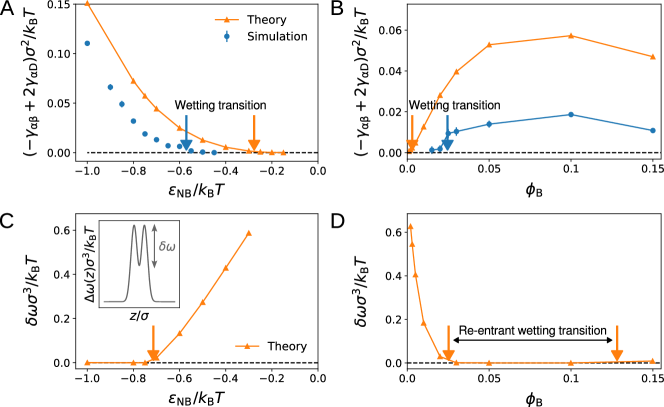
Figure 5: Identifying surfactant-dependent wetting transitions. (A) The difference between the non-wetting and wetting surface tensions, $2\gamma_{\alpha\text{D}}-\gamma_{\alpha\beta}$, as a function of the N–B interaction, $\epsilon_{\text{NB}}$, at constant $\phi_{\text{B}}=0.1$. Results are shown for simulations (blue circles) and CDFT calculations (orange triangles). Arrows indicate the locations of the wetting transition, where the surface-tension difference equals zero to within twice the statistical uncertainty, inferred from both methods. Statistical uncertainties are comparable to the symbol size. (B) The surface-tension difference as a function of the B-species volume fraction, $\phi_{\text{B}}$, at constant $\epsilon_{\text{NB}}=-0.75\,k_{\text{B}}T$. (C–D) The location of the wetting transition can also be estimated from CDFT by examining where the double peaks of the excess free-energy profile merge (see inset of C). In D, this method predicts a re-entrant wetting transition at constant $\epsilon_{\text{NB}}=-0.75\,k_{\text{B}}T$. All calculations assume that the homotypic interaction is $\epsilon_{\text{BB}}=0$.

Despite the approximations inherent to our CDFT approach, we find semi-quantitative agreement between the predicted and simulated concentration profiles (Fig. 4A). The interfaces predicted by CDFT are slightly broader and tend to exaggerate the B-species enrichment at the interface relative to the simulation results. From CDFT calculations, we directly obtain predictions for the excess free energy across each interface, $\Delta\omega(z)$ (Fig. 4B), from which we can predict the associated surface tension via Eq. (9). In the case of the $\alpha$–dilute interface, the excess free energy profile is asymmetric about the Gibbs dividing surface, with the maximum shifted toward the dilute phase.

The behavior of the B species near each interface is more clearly seen in the three-dimensional (N1, N2, B) concentration space (Fig. 4C–E). The enrichment of the B species relative to its concentration in either the condensed or dilute phase results in a marked deviation from the linear-path approximation (dashed lines in Fig. 4C–E). Consequently, the excess free energy predicted by the full CDFT approach for the $\alpha$–$\beta$ interface shown in Fig. 4A–B is substantially lower than that predicted by the linear-path constraint. Because the deviation from the linear-path approximation is greater for the $\alpha$–$\beta$ interface than the $\alpha$–dilute interface, the linear-path approximation tends to mischaracterize wetting conditions as non-wetting. By contrast, MFEP calculations (dot-dashed lines in Fig. 4C–E) exaggerate the enrichment of B molecules at all interfaces, and we find that the MFEP between the $\alpha$ and $\beta$ phases in concentration space actually passes through the dilute phase. The full CDFT approach, which most closely matches the simulation results, is intermediate between these limiting cases, exhibiting a reduction of the N1 and N2 concentrations at the interface without passing through the dilute phase (Fig. 4D). We stress that these predictions are dependent on our regularization approach for the $\bm{m}$-matrix (see Sec. IV), without which CDFT would yield diverging interfacial fluctuations for the parameters used in Fig. 4. Overall, these comparisons demonstrate the semi-quantitative accuracy of the full CDFT approach and highlight potential shortcomings of the CH formula, Eq. (11), in multicomponent settings.

V.2 Computing the wetting transition

To determine how the equilibrium multiphase morphology changes with the concentration and heterotypic interactions of the B species, we compute the surface-tension difference $-\gamma_{\alpha\beta}+2\gamma_{\alpha\text{D}}$ using both simulation results and CDFT calculations (Fig. 5A–B). A positive surface-tension difference, $-\gamma_{\alpha\beta}+2\gamma_{\alpha\text{D}}>0$, indicates a stable wetting interface between the $\alpha$ and $\beta$ phases. From our simulation results, we compute this quantity based on the PMF minimum (Sec. III), and we identify the wetting transition where the PMF minimum becomes statistically indistinguishable from zero (blue arrows in Fig. 5A–B). In our CDFT calculations, the $\alpha$–$\beta$ interface spontaneously relaxes to two dense–dilute interfaces when a non-wetting configuration is predicted, in which case we obtain a near-zero value for the surface-tension difference due to finite numerical precision (see Appendix B). We therefore identify the CDFT wetting transition by comparing the surface-tension difference to the numerical precision (orange arrows in Fig. 5A–B).

Our simulations and CDFT calculations predict qualitatively similar behavior for the surface-tension difference and the location of the wetting transition. In particular, both simulation and theory predict that the surface-tension difference tends to increase, leading to a stable wetting configuration, with decreasing $\epsilon_{\text{NB}}$ and increasing $\phi_{\text{B}}$. However, the wetting transition occurs at weaker N–B interactions and lower B concentrations in the CDFT theory. This quantitative discrepancy likely arises from the assumptions invoked in theory, including the mean-field free-energy density, which results in a reduced critical interaction strength; the square-gradient approximation for the grand-potential functional; the approximate $\bm{m}$-matrix; and neglect of concentration fluctuations at the interfaces. Nonetheless, it is interesting that the equilibrium concentration profiles predicted by CDFT appear to be in much closer agreement with the simulation results than the surface-tension differences. This comparison suggests that the key shortcoming of the CDFT theory lies in the treatment of interfacial fluctuations, which we expect to have stronger effects on surface free energies than static concentration profiles.

Motivated by this observation, we consider an alternative strategy for predicting the wetting transition from our CDFT calculations. Specifically, we reason that the equilibrium excess free-energy profile between the $\alpha$ and $\beta$ phases should exhibit a single peak at the Gibbs dividing surface in the case of a wetting configuration. By contrast, a non-wetting configuration requires spatially separated $\alpha$–dilute and $\beta$–dilute interfaces, and thus corresponds to an excess free-energy profile with two distinct peaks. We indeed observe this expected behavior in our CDFT calculations, except in scenarios where the predicted surface tension difference is positive yet near-zero. In these situations, the equilibrium excess free-energy profile is doubly peaked (inset of Fig. 5C), while the two peaks tend to merge as the N–B interaction strengthens (Fig. 5C). Reasoning that a doubly peaked excess free-energy profile is unlikely to be stable with respect to concentration fluctuations that are not explicitly accounted for in the theory, we propose that this prediction, characterized by the peak-to-trough height $\delta\omega$ (inset of Fig. 5C), can be taken as an empirical indicator of a stable non-wetting configuration (Fig. 5C–D). Overall, we find that this criterion yields more accurate predictions with respect to our simulation results than direct calculation of the CDFT surface-tension difference. This observation points to the important role of interfacial fluctuations in determining the equilibrium multiphase morphology in our model. Furthermore, we note that this empirical criterion is appealing from a computational point of view, since it is less sensitive to numerical precision, and thus requires fewer optimization iterations to converge, than the CDFT surface-tension difference.

V.3 Design rules for regulating multiphase condensate morphology via programmable surfactants

The equilibrium multiphase morphology can be summarized in a wetting phase diagram (Fig. 6A). Here we plot separate curves predicting the discontinuous wetting transition based on simulations, the CDFT surface-tension difference, and the CDFT excess free-energy profile structure. The region of parameter space below each curve in the $\epsilon_{\text{NB}}$–$\phi_{\text{B}}$ plane corresponds to an equilibrium wetting configuration, where a docked multiphase morphology is thermodynamically stable. We also report the phase diagram for a model in which the B species interacts via weak, attractive homotypic interactions, such that $\epsilon_{\text{BB}}=-0.5\,k_{\text{B}}T$ (Fig. 6B). As noted above, the CDFT surface-tension differences tend to underpredict the $\epsilon_{\text{NB}}$ interaction strength required to trigger the wetting transition, while the empirical criterion based on the excess free-energy profile predicts a phase boundary in closer agreement with the simulation results. Nonetheless, both CDFT-based methods capture the qualitative shape of the phase diagram with and without homotypic interactions.

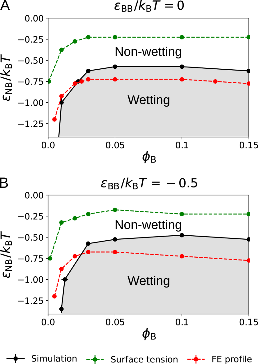
Figure 6: Wetting phase diagrams with and without homotypic surfactant interactions. Phase diagrams are shown as a function of the B-species volume fraction, $\phi_{\text{B}}$, and the heterotypic N–B interaction energy, $\epsilon_{\text{NB}}$, for scenarios (A) without homotypic interactions, $\epsilon_{\text{BB}}=0$, and (B) with weak homotypic B–B interactions, $\epsilon_{\text{BB}}=-0.5\,k_{\text{B}}T$. Shaded regions indicate wetting conditions. Phase boundaries are predicted from simulation results (black points), CDFT surface-tension calculations (green points), and the shapes of the CDFT excess free-energy (FE) profiles (red points).

The wetting phase diagrams presented in Fig. 6 exhibit a number of striking features. First, there is a minimum heterotypic interaction strength, $|\epsilon_{\text{NB}}^{*}|$, required for a stable wetting configuration. Stable docked morphologies therefore cannot occur for $\epsilon_{\text{NB}}>\epsilon_{\text{NB}}^{*}$, regardless of the B-species concentration. In this model, we find that $\epsilon_{\text{NB}}^{*}\approx-0.6\,k_{\text{B}}T$, which is considerably weaker than the critical interaction strength of the cubic lattice gas model [23]. Second, the wetting transition passes through $\epsilon_{\text{NB}}^{*}$ at a finite B-species volume fraction. This observation implies that the wetting transition is re-entrant for values of $\epsilon_{\text{NB}}$ close to $\epsilon_{\text{NB}}^{*}$, where increasing $\phi_{\text{B}}$ at a constant heterotypic interaction strength leads the system to transition from the non-wetting regime to the wetting regime, and then back to the wetting regime at high B-species concentrations (see, e.g., Fig. 5D). Third, the phase boundary extends to low B-species volume fractions, on the order of only a few percent. Importantly, at dilute B-species concentrations, the heterotypic interaction strength required to trigger the wetting transition weakens rapidly with increasing $\phi_{\text{B}}$. By contrast, the phase boundary is comparably insensitive to $\phi_{\text{B}}$ near $\epsilon_{\text{NB}}^{*}$.

Finally, we observe that the homotypic B–B interactions have only a minor quantitative effect on the wetting phase diagram. This finding indicates that weak homotypic interactions among surfactant-like species play a secondary role in modulating multiphase condensate morphology. However, there are slight differences between the phase diagrams. On one hand, introducing homotypic B–B interactions reduces the minimum required interaction strength, $|\epsilon_{\text{NB}}^{*}|$, by a small amount. On the other hand, at dilute B-species concentrations, the wetting phase boundary is shifted to slightly stronger heterotypic N–B interactions.

Taken together, these observations establish general design rules for programmable surfactants. Most importantly, our results indicate that relatively low concentrations of a surfactant-like species ($\phi_{\text{B}}\gtrsim 0.03$) and relatively weak heterotypic interactions ($\epsilon_{\text{NB}}\lesssim-0.6\,k_{\text{B}}T$) are sufficient to trigger a wetting transition in a multicomponent, multiphase mixture. We note that the results presented in these phase diagrams are insensitive to changes in the concentrations of the N1 and N2 species, as these changes do not substantially affect the compositions of the bulk $\alpha$ and $\beta$ phases when the B species is dilute. Altering the concentrations of the N1 and N2 species does change the volume fractions of the $\alpha$ and $\beta$ phases, however. Although the wetting phase boundary is independent of the volume fractions of the condensed phases, the equilibrium multiphase morphology may transition from partial wetting (i.e., a docked configuration) to complete wetting (i.e., a core–shell structure) when the $\alpha$ and $\beta$-phase volume fractions differ substantially [15, 16].

V.4 Understanding programmable surfactant design rules using an adsorption model

To gain a deeper understanding of these empirical design rules, we introduce a simple adsorption model that recapitulates the key features of the wetting phase diagrams (Fig. 6). We examine the interplay between the parameters $\epsilon_{\text{NB}}$, $\epsilon_{\text{BB}}$, and $\phi_{\text{B}}$ by considering a Langmuir-like model [37] in which the B species acts as the adsorbate. We therefore assume that each fluctuating interface between a pair of phases can be described by a two-dimensional lattice gas with B-species occupancy $\phi_{\text{B}}^{(\text{i})}$.

We first consider the system without homotypic B-species interactions ($\epsilon_{\text{BB}}=0$). The surface excess grand potential due to the presence of the interface [26] takes the form

$$\frac{\Omega^{\text{ex}}(\phi^{(\text{i})}_{\text{B}})\sigma^{2}}{Ak_{\text{B}}T}=h(\phi^{(\text{i})}_{\text{B}})-\frac{\Delta S(\phi^{(\text{i})}_{\text{B}})}{Ak_{\text{B}}}-\frac{\mu_{\text{B}}}{k_{\text{B}}T}\phi^{(\text{i})}_{\text{B}},$$ (12)

where $A$ is the interfacial area. The first enthalpic term is linearly related to the occupied volume fraction in the mean-field approximation, $h(\phi^{(\text{i})}_{\text{B}})=-a\phi^{(\text{i})}_{\text{B}}+b$,. For a surfactant-like adsorbate, $a$ is positive. Meanwhile, $b$ represents the enthalpic penalty due to the creation of an interface from a bulk condensed phase and is independent of $\phi^{(\text{i})}_{\text{B}}$. The entropic contribution, $\Delta S(\phi^{(\text{i})}_{\text{B}})/Ak_{\text{B}}=-\phi^{(\text{i})}_{\text{B}}\ln\phi^{(\text{i})}_{\text{B}}-(1-\phi^{(\text{i})}_{\text{B}})\ln(1-\phi^{(\text{i})}_{\text{B}})+s$, accounts for the in-plane configurational entropy of the adsorbed B molecules as well as the entropic penalty, $s$, due to capillary fluctuations. Finally, $\mu_{\text{B}}$ is the B-species chemical potential. Since the dense phase is in coexistence with the approximately ideal dilute phase, we have $\mu_{\text{B}}/k_{\text{B}}T\simeq\ln\phi^{(\text{D})}_{\text{B}}$, where $\phi^{(\text{D})}_{\text{B}}$ is the B-species volume fraction in the dilute phase. Minimizing the surface excess grand potential, Eq. (12), with respect to $\phi^{(\text{i})}_{\text{B}}$, we arrive at a Langmuir adsorption isotherm for the B species,

$$\phi^{(\text{i})}_{\text{B,eq}}=\frac{K}{1+K},$$ (13)

where $K\equiv\phi^{(\text{D})}_{\text{B}}e^{a}$. This prediction agrees well with the enrichment of B molecules at $\alpha$–$\beta$ interfaces in our simulations (Fig. 7A). The surface tension in this model can then be computed from the equilibrium surface excess grand potential,

$$\gamma\equiv\frac{\Omega^{\text{ex}}(\phi^{(\text{i})}_{\text{B,eq}})}{A}=\frac{k_{\text{B}}T}{\sigma^{2}}[b-s-\ln(1+K)].$$ (14)

We now apply Eq. (14) to both the $\alpha$–$\beta$ and the $\alpha$–dilute interfaces. The $\phi^{\text{(i)}}_{\text{B}}$-independent enthalpic contribution must be the same regardless of the distance between the $\alpha$ and $\beta$-phase interfaces, so that ${b_{\alpha\beta}=2b_{\rm\alpha D}}$. By contrast, the entropic contribution due to capillary fluctuations depends on whether one or two distinct interfaces are present between the $\alpha$ and $\beta$ phases. We therefore define the dimensionless entropic difference ${\Delta s\equiv 2s_{\rm\alpha D}-s_{\alpha\beta}}$, which is necessarily positive and increases with the interfacial roughness. In a wetting case,

$$\gamma_{\rm\alpha\beta}-2\gamma_{\rm\alpha D}=\frac{k_{\text{B}}T}{\sigma^{2}}\left[\Delta s+\ln\frac{(1+K_{\rm\alpha D})^{2}}{1+K_{\rm\alpha\beta}}\right]<0.$$ (15)

Eq. (15) predicts a wetting phase boundary that is quadratic with respect to $\phi^{(\text{i})}_{\text{B}}$ (see Appendix D), which indicates that wetting can only occur when [38]

$$a_{\rm\alpha D}-a_{\rm\alpha\beta}<\ln\frac{1-\sqrt{1-e^{-\Delta s}}}{2}.$$ (16)

Because the coefficients $a_{\rm\alpha D}$ and $a_{\rm\alpha\beta}$ reflect the enthalpic contribution due to the adsorption of B molecules, we assume that the left-hand side of Eq. (16) is roughly proportional to $\epsilon_{\text{NB}}$. Moreover, by making the approximation ${a_{\rm\alpha\beta}\simeq 2a_{\rm\alpha D}}$, which implies that a B molecule engages in twice as many N–B interactions at an $\alpha$–$\beta$ interface, we obtain a relation between $\phi^{(\text{D})}_{\text{B}}$ and $\Delta s$ at the minimum binding strength, $|\epsilon_{\text{NB}}^{*}|$, on the wetting phase boundary,

$$\left.\phi^{(\text{D})}_{\text{B}}\right|^{*}=\frac{-(1-e^{-\Delta s})+\sqrt{1-e^{-\Delta s}}}{2}.$$ (17)

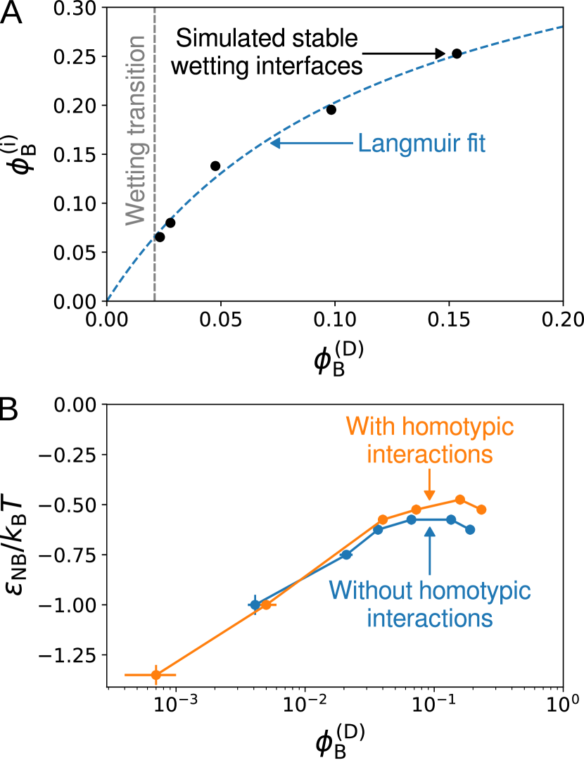
Figure 7: An adsorption model predicts qualitative features of the wetting transition. (A) The enrichment of B molecules at the $\alpha$–$\beta$ interface can be described by a Langmuir isotherm. Here, simulation measurements of the B-species enrichment ($\epsilon_{\text{NB}}=-0.75k_{\text{B}}T$, $\epsilon_{\text{BB}}=0$) are fit to a Langmuir isotherm, Eq. (13), with fitting parameter $a_{\alpha\beta}=2.1$ and an empirical scaling factor of $0.45$. (B) Wetting phase boundaries with and without homotypic interactions as a function of the B-species volume fraction in the dilute phase (replotted simulation data from Fig. 6). The model predicts the nonmonotonicity of the phase boundary, the asymptotic behavior at low $\phi_{\text{B}}^{(\text{D})}$, and the increase of the maximum N–B interaction on the phase boundary, $\epsilon_{\text{NB}}^{*}$, due to homotypic B–B interactions.

Importantly, Eqs. (15)–(17) predict a non-monotonic wetting phase boundary, with a re-entrant wetting transition at constant $\epsilon_{\text{NB}}$, as observed in our simulations. We can also estimate $\phi^{(\text{D})}_{\text{B}}|^{*}$ by computing $\Delta s$ directly from our simulated PMF at zero B-species concentration, where $k_{\text{B}}T\Delta s/\sigma^{2}=\gamma_{\rm\alpha\beta}-2\gamma_{\rm\alpha D}\simeq F(\Delta r=0)/A$. From Fig. 3B, we find $\Delta s\approx 0.15$, which, according to Eq. (17), suggests that $\phi^{(\text{D})}_{\text{B}}|^{*}\simeq 0.12$. This prediction is also in reasonable agreement with our simulation results (Fig. 7B). Finally, in the low-concentration and high-affinity regime, $e^{a_{\alpha\beta}-a_{\alpha\text{D}}}\gg e^{\Delta s}$, we obtain an asymptotic formula for the low-concentration phase boundary,

$$\ln\phi^{(\text{D})}_{\text{B}}+a_{\alpha\beta}=\ln(e^{\Delta s}-1).$$ (18)

The logarithmic dependence on $\phi_{\text{B}}^{(\text{D})}$ in Eq. (18) explains the sensitivity of the wetting transition to the B-species concentration under these conditions (Fig. 7B), where we see that $\partial a_{\alpha\beta}/\partial\ln\phi^{(\text{D})}_{\text{B}}\propto\partial\beta\epsilon_{\text{NB}}/\partial\ln\phi^{(\text{D})}_{\text{B}}$ is roughly constant. The behavior in the low-concentration, high-affinity regime can therefore be interpreted as a competition between capillary fluctuations and the free-energy change when adsorbing a B molecule to the $\alpha$-$\beta$ interface.

We now consider systems with homotypic interactions ($\epsilon_{\text{BB}}<0$). In this scenario, the mean-field approximation for the enthalpic contribution in Eq. (12) acquires an extra term $-a^{\prime}(\phi_{\text{B}}^{(\text{i})})^{2}$, where $a^{\prime}>0$, that accounts for B–B interactions at the interface. The chemical potential $\mu_{\text{B}}$ similarly picks up a term that is proportional to $\phi_{\text{B}}^{(\text{D})}$, since the B molecules can also attract one another in the dilute phase. The effects of these modifications can then be predicted by perturbing the $\epsilon_{\text{BB}}=0$ results (see Appendix D). In the low-concentration limit, both $\phi_{\text{B}}^{(\rm i)}$ and $\phi_{\text{B}}^{(\text{D})}$ are small, so that the asymptotic behavior given by Eq. (18) remains unchanged; this prediction is confirmed by plotting the wetting phase boundary as a function of $\phi_{\text{B}}^{(\text{D})}$ in Fig. 7B. However, near $\phi^{(\text{D})}_{\text{B}}|^{*}$, the perturbation due to $a^{\prime}$ is non-negligible. Specifically, turning on homotypic B–B interactions results in a change to the surface tension difference,

$$\Delta(\gamma_{\rm\alpha\beta}-2\gamma_{\rm\alpha D})|^{*}=-\frac{2K^{2}_{\rm\alpha D}|^{*}}{(1+K^{*}_{\rm\alpha D})^{2}}a^{\prime}<0,$$ (19)

at the maximum N–B interaction, $\epsilon_{\text{NB}}^{*}$, on the phase boundary. The sign of Eq. (19) indicates that homotypic B–B interactions weaken the required N–B interaction strength, resulting in an increased $\epsilon_{\text{NB}}^{*}$. This prediction is also agrees with our simulation results (Fig. 7B).

In summary, this analytical model explains all the essential features of our wetting phase diagrams, including the re-entrant wetting transition and the low-concentration asymptotic behavior. Notably, these predictions are obtained without assuming specific values of the coefficients in the mean-field adsorption model. We therefore expect that the design rules that we have derived for programmable surfactants hold beyond the specific lattice model that we have simulated in this work.

VI Discussion

In this work, we consider a simplified, coarse-grained model of a “programmable surfactant” in a multicomponent biomolecular mixture. Our central results are a set of design rules for controlling multiphase condensate morphologies, which are summarized in the wetting phase diagrams presented in Fig. 6. Most importantly, these phase diagrams demonstrate that surprisingly low concentrations of a weakly interacting programmable surfactant can induce a discontinuous transition from non-wetting (i.e., “dispersed”) to wetting (i.e., “docked” or “core–shell”) configurations. More precisely, we find that the heterotypic interactions between the surfactant-like species and the majority component(s) of the condensed phases must exceed a relatively weak binding strength. However, given heterotypic interactions that are slightly stronger than this threshold value, a surfactant volume fraction of only a few percent is needed to trigger the wetting transition. These observations imply that relatively small changes to the state of the system—either small adjustments to the concentrations or heterotypic binding strengths of the surfactant-like species—can alter the equilibrium morphology of a multiphase condensate.

We find that the qualitative features of the wetting phase diagrams agree between our molecular simulation results and the predictions of a classical density functional theory (CDFT) approach. From our molecular simulations, we predict the wetting behavior in the thermodynamic limit using measurements of the potential of mean force between condensates in a finite-size system. In the CDFT approach, we minimize an approximate grand-potential functional to obtain predicted equilibrium concentration profiles in the vicinity of the condensate interfaces. Although the predicted concentration profiles are in semi-quantitative agreement with the simulation results, the wetting phase diagrams agree only qualitatively. Nonetheless, this qualitative agreement represents a substantial improvement over a multicomponent generalization of the Cahn–Hilliard formula and demonstrates that our CDFT approach captures the relevant physics despite not accounting for concentration fluctuations and capillary waves at the interfaces. Moreover, the qualitative agreement that we obtain between the predictions of a simplified adsorption model and our detailed calculations suggests that the design rules that we have extracted from the wetting phase diagrams are likely to apply much more generally to related models of programmable surfactants with different molecular details. For example, our simulation methods and theoretical framework could be applied to more sophisticated models of biomolecules with directional as opposed to isotropic interactions, and we anticipate that our design rules would be qualitatively unaffected.

Returning to the stress granule (SG)/P-body (PB) system that motivated our model, we propose that the insights gained from our calculations can be applied directly to protein/RNA interaction networks that underlie the phase behavior of multiphase biomolecular condensates. The key step lies in coarse-graining the interaction network to identify potential surfactant-like species, which should interact with protein/RNA components in multiple, distinct condensed phases. Such species are likely to be situated as “bridges” between strongly interacting portions of the network [21]. For example, in the SG/PB system [21], the protein DDX6 (Fig. 1A) is an obvious candidate, as it is weakly recruited to both condensates. Our model predicts that this species should be weakly enriched at SG/PB interfaces in the endogenous system, which exhibits a stable docked morphology. In future work, we will examine theoretical methods for identifying surfactant-like species on the basis of the interaction network structure and experimentally determined binding affinities and expression levels. In light of our current results, the requirements of moderate binding strengths and low molecular concentrations suggest that this proposed mechanism of a molecular “switch” for controlling intracellular condensate morphologies is likely to be biologically relevant. Further experiments are needed to test the detailed predictions of our model.

Finally, we note that this proposed mechanism is not limited to naturally occurring biomolecular systems. Low-concentration, surfactant-like molecular switches may also be useful for tuning multiphase morphologies in materials engineering, where approaches that do not require substantial changes to the bulk properties of the coexisting phases are similarly desirable. For example, the phase behavior of multiphase DNA “nanostar” liquids [39] can also be interpreted in terms of an interaction network, in which “cross-linker” nanostars can be engineered to play the role of the molecular switch. This nanostar system and similar examples of programmable soft matter [40] would be ideal opportunities to test our predictions experimentally and to apply the design rules developed in this work.

Appendix A Phase-coexistence calculations

We solve for phase coexistence in the regular solution model (Sec. IV) following the numerical strategy developed in Ref. [22]. Specifically, we solve for the molecular volume fractions, $\{\vec{\phi}^{(k)}\}$, and the mole fractions of the coexisting phases, $\{x^{(k)}\}$, given the total molecular volume fractions, $\vec{\phi}_{\operatorname{tot}}$. Mass conservation requires that

$$\vec{\phi}_{\text{tot}}=\sum^{m}_{k=1}x^{(k)}\vec{\phi}^{(k)},$$ (20)

if there are $m$ phases in coexistence.

We now consider the conditions for phase equilibrium. The grand-potential density is related to the free-energy density via ${\omega_{0}=f_{0}-\sum_{i=1}^{N}(\partial f_{0}/\partial\phi_{i})\phi_{i}}$, where the chemical potentials of the non-solvent molecular species are ${\mu_{i}=\sigma^{3}\partial f_{0}/\partial\phi_{i}}$. Coexisting phases are located at minima of $\omega_{0}$, ensuring that all components have equal chemical potentials in all phases. Phase equilibrium also requires equal pressures across all coexisting phases, implying that the $\omega_{0}(\vec{\phi})$ has the same value at all local minima. Together, these conditions require

$$\omega_{0}(\vec{\phi}^{(k)})=\min\omega_{0}(\vec{\phi};\vec{\mu}).$$ (21)

We solve Eq. (21) numerically by minimizing the norm of the residual errors of Eq. (20) and Eq. (21) iteratively. At each iteration, we first locate the local minima of the grand potential, $\vec{\phi}^{(k)}=\arg\min_{\vec{\phi}}\omega_{0}(\vec{\phi};\vec{\mu})$ for all phases $k=1,\ldots,m$, using the Nelder-Mead method [41]. We then update $\vec{\mu}$ and $\{x^{(k)}\}$ using the modified Powell method [42].

Success of this optimization procedure requires that the initial estimates of $\{\vec{\phi}^{(k)}\}$ are not too far from the values at coexistence. We obtain an initial guess for $\{\vec{\phi}^{(k)}\}$ from the convex hull method [15, 22], in which we locate the convex hull of points on a discretized $(N+1)$-dimensional free energy surface. We initialize our optimization procedure with $N+1$ vectors $\{\vec{\phi}^{(k)}\}$ that correspond to the vertices of the convex hull facet that encompasses $\vec{\phi}_{\text{tot}}$. From the linear equation that defines this facet, we also obtain initial guesses for $\vec{\mu}$ and $\{x^{(k)}\}$. When the number of coexisting phases $m$ is less than $N+1$, some of the $N+1$ vectors $\{\vec{\phi}^{(k)}\}$ are identical to within numerical tolerance after optimization; in this case, we restart the optimization procedure with a unique set of vectors and the corresponding $\vec{\mu}$ and $\{x^{(k)}\}$. In this way, we determine the number of coexisting phases, $m$, as well as the molecular volume-fraction vectors, $\{\vec{\phi}^{(k)}\}$, and chemical potentials, $\vec{\mu}$, at phase coexistence.

Appendix B Numerical solution of the CDFT Euler–Lagrange equation

To minimize the grand-potential functional in Eq. (5), we employ a numerical approach based on gradient descent. We first discretize the $z$ coordinate, oriented perpendicular to the planar interface between phases, as $\{z_{k}\}$ for $k=1,2,\ldots,n$. As a result, the integration in Eq. (5) becomes a summation, and the grand-potential functional becomes a function of $n$ $N$-dimensional vectors $\vec{\phi}_{k}\equiv\vec{\phi}(z_{k})$. Using the central difference formula for differentiation, Eq. (5) becomes

$$\frac{\Omega}{Ah}=\sum^{n-1}_{k=2}\!\left[\omega_{0}(\vec{\phi}_{k})\!+\!\frac{(\vec{\phi}_{k+1}\!-\!\vec{\phi}_{k-1}\!)^{\top}\cdot\bm{m}\cdot(\vec{\phi}_{k+1}\!-\!\vec{\phi}_{k-1}\!)}{2(2h)^{2}}\right]\!,$$ (22)

where $h\equiv z_{k+1}-z_{k}$ is the discretization interval. We fix the vectors $\vec{\phi}_{k}$ at the two points closest to each boundary, $k=1,2,n-1,$ and $n$, to be equal to the bulk phase densities. In all calculations, we set $h=0.02\sigma$ and $n=1004$. These choices separate the bulk-phase boundary conditions by a distance of $20\sigma$, which is much greater than the typical interfacial width (Fig. 2B).

We then apply gradient descent to minimize the discretized grand potential, Eq. (22), by calculating the partial derivatives $\partial\Omega/\partial\vec{\phi}_{k}$. At each optimization step $l$, the densities are updated according to

$$\vec{\phi}^{\;(l+1)}_{k}=\vec{\phi}^{\;(l)}_{k}-\lambda\left(\frac{\partial\Omega}{\partial\vec{\phi}_{k}}\right)_{\!\vec{\phi}^{\,(l)}}\!,$$ (23)

where $\lambda$ controls the step size. We choose $10^{-3}$ as the initial value of $\lambda$ and reduce it by half if an attempted step increases the grand potential. We initialize this optimization algorithm using an interface with a width of $4\sigma$ and a piecewise-linear spatial variation of the molecular volume fractions. The algorithm terminates when the norm of the gradient falls below a threshold value, $10^{-3}$, at which point we take $\vec{\phi}(z_{k})$ to be the equilibrium profile.

To verify the convergence of this algorithm, we perturb the concentration profiles by moving the $\alpha$ and $\beta$ interfaces apart by $0.04\sigma$ and then restarting the optimization algorithm. In a wetting scenario, the profile converges back to the result of the original optimization. However, in a non-wetting scenario, the profile remains close to the perturbed profile, consistent with an unstable interface. In practice, we compare the norms of the distances between the re-optimized, perturbed, and originally optimized profiles to verify the optimization result.

Appendix C Minimum free-energy path calculations

We calculate the minimum free-energy path (MFEP) on the bulk excess free-energy landscape, $\Delta\omega_{0}(\vec{\phi})$ (see Sec. IV.3) using a direct implementation of the zero-temperature string method [36]. For a discussion of the algorithmic details, we refer the reader to Ref. [36]. We use the same notations and terminology here as in the original paper.

We use a total of $N=100$ points on the string between two local minima on the bulk excess free energy surface. The algorithm iteratively updates the points in a two-step manner. In the evolution step, the points evolve according to the gradient descent method, as in Eq. (23), where $\Delta t$ controls the step size. Here we use the forward Euler method with $\Delta t=5\times 10^{-4}$. Then in the reparameterization step, we reparameterize the string such that the $N$ points are equally spaced with respect to arc length along the string. We check for convergence by measuring the norm of the displacement of all points from their positions in the previous iteration. We set the tolerance for convergence to be $\text{TOL}=10^{-4}$.

Appendix D Fluctuating-interface adsorption model

In this section, we detail the essential steps to bridge the gaps between Eq. (15) and the subsequent results in Sec. V.4 of the main text. Explicitly expressing the wetting condition in Eq. (15) leads to

$$(\phi^{(\text{D})}_{\text{B}})^{2}e^{2a_{\rm\alpha D}}+\phi^{(\text{D})}_{\text{B}}(2e^{a_{\rm\alpha D}}\!-\!e^{a_{\rm\alpha\beta}-\Delta s})+1\!-\!e^{-\Delta s}<0.$$ (24)

The discriminant of this quadratic function must be positive, such that $(2e^{a_{\rm\alpha D}}-e^{a_{\rm\alpha\beta}-\Delta s})^{2}-4e^{2a_{\rm\alpha D}}(1-e^{-\Delta s})>0$. Here, both $a_{\rm\alpha D}$ and $a_{\alpha\beta}$ are expected to be proportional to the N–B binding energy, $\epsilon_{\text{NB}}$. In addition, physical values of $\phi^{(\text{D})}_{\text{B}}$ must be between 0 and 1. With these conditions, Eq. (24) allows us to predict the weakest N–B binding strength for a wetting interface. The volume fraction at this binding strength is

$$\phi^{(\text{D})}_{\text{B}}\big{|}^{*}=e^{-a_{\rm\alpha D}}\sqrt{1-e^{-\Delta s}}.$$ (25)

Then, by making the approximation ${a_{\rm\alpha\beta}\simeq 2a_{\rm\alpha D}}$, we are able to express these quantities in terms of $\Delta s$ at the weakest N–B binding strength, $|\epsilon_{\text{NB}}^{*}|$, on the wetting phase boundary,

$$a^{*}_{\rm\alpha D} =\ln 2+\ln[e^{\Delta s}+\sqrt{e^{\Delta s}(e^{\Delta s}-1)}],$$ (26)

$$K^{*}_{\rm\alpha D} =\sqrt{1-e^{-\Delta s}},$$ (27)

$$\phi^{({\rm i,\alpha\beta})}_{\text{B}}\big{|}^{*} =2\phi^{({\rm i,\alpha D})}_{\text{B}}\big{|}^{*}.$$ (28)

According to Eq. (26), the minimum binding strength $|\epsilon_{\text{NB}}^{*}|$ increases with $\Delta s$, since $a_{\rm\alpha D}\propto|\epsilon_{\text{NB}}|$. As $\Delta s$ increases, the B-species volume fraction in the dilute phase, $\phi^{(\text{D})}_{\text{B}}\big{|}^{*}$, first increases until reaching a maximum value of 0.125 at $K^{*}_{\rm\alpha D}=0.5$, as evidenced by substitution of Eq. (27) into Eq. (17). $\phi^{(\text{D})}_{\text{B}}\big{|}^{*}$ then decreases with $\Delta s$ at larger $\Delta s$. The wetting phase boundary is always non-monotonic for a positive $\Delta s$. These observations suggest that an accurate treatment of the capillary fluctuations, quantified here by $\Delta s$, is essential for obtaining an accurate prediction of $|\epsilon_{\text{NB}}^{*}|$; this interpretation is consistent with the quantitative differences between our CDFT and simulation results in Fig. 6.

Next, we extend this adsorption model to incorporate homotypic B–B interactions. To this end, we modify the mean-field expressions for the enthalpic contribution to the surface excess grand potential and the chemical potential in Eq. (12),

$$h(\phi^{(\rm i)}_{\text{B}}) =-a^{\prime}(\phi^{(\rm i)}_{\text{B}})^{2}-a\phi^{(\rm i)}_{\text{B}}+b,$$ (29)

$$\mu_{\text{B}}/k_{\text{B}}T =\ln\phi^{(\text{D})}_{\text{B}}-c\phi^{(\text{D})}_{\text{B}},$$ (30)

where $a^{\prime}$ and $c$ are positive constants that are expected to be proportional to $|\epsilon_{\text{BB}}|$. We can then show that these additional terms in Eq. (29) and Eq. (30) lead to a decrease in $(\gamma_{\alpha\beta}-2\gamma_{\rm\alpha D})|^{*}$ by considering perturbations to the $\epsilon_{\text{BB}}=0$ case. Comparison with Eq. (12) shows that these additional terms effectively alter the parameter $a$ in the original model by

$$\Delta a=a^{\prime}\phi^{(\rm i)}_{\text{B}}-c\phi^{(\rm D)}_{\text{B}}.$$ (31)

According to Eq. (14), introducing the perturbation $\Delta a$ changes the surface tension by an amount

$$\Delta\gamma=-\phi^{(\rm i)}_{\text{B}}\Delta a=-\phi^{(\rm i)}_{\text{B}}(a^{\prime}\phi^{(\rm i)}_{\text{B}}-c\phi^{(\rm D)}_{\text{B}}),$$ (32)

and thus the surface tension difference by an amount

$$\Delta(\gamma_{\rm\alpha\beta}-2\gamma_{\rm\alpha D})= -[(\phi^{({\rm i,\alpha\beta})}_{\text{B}})^{2}-2(\phi^{({\rm i,\alpha D})}_{\text{B}})^{2}]a^{\prime}$$ (33)

$$+(\phi^{({\rm i,\alpha\beta})}_{\text{B}}-2\phi^{({\rm i,\alpha D})}_{\text{B}})\phi^{(\text{D})}_{\text{B}}c.$$

Again assuming that ${a_{\rm\alpha\beta}\simeq 2a_{\rm\alpha D}}$, we apply these results to the minimum binding strength, $|\epsilon_{\text{NB}}^{*}|$, on the $\epsilon_{\text{BB}}=0$ wetting phase boundary. Simplifying Eq. (33) using Eq. (13) and Eq. (28), we find that the term involving the parameter $c$ cancels out, and we arrive at Eq. (19). The fact that $\Delta(\gamma_{\rm\alpha\beta}-2\gamma_{\rm\alpha D})|^{*}$ is negative, regardless of specific choices for the parameters $a^{\prime}$ and $c$, indicates that the minimum binding strength $|\epsilon^{*}_{\text{NB}}|$ is reduced in the presence of homotypic B–B interactions compared to the $\epsilon_{\text{BB}}=0$ scenario. Thus, this model predicts that $\epsilon_{\text{NB}}^{*}$ increases for $\epsilon_{\text{BB}}<0$.

References

- Hyman et al. [2014] A. A. Hyman, C. A. Weber, and F. Jülicher, Liquid–liquid phase separation in biology, Annu. Rev. Cell Dev. Biol. 30, 39 (2014).
- Boeynaems et al. [2018] S. Boeynaems, S. Alberti, N. L. Fawzi, T. Mittag, M. Polymenidou, F. Rousseau, J. Schymkowitz, J. Shorter, B. Wolozin, L. Van Den Bosch, P. Tompa, and M. Fuxreiter, Protein phase separation: A new phase in cell biology, Trends Cell Biol. 28, 420 (2018).
- Wheeler and Hyman [2018] R. J. Wheeler and A. A. Hyman, Controlling compartmentalization by non-membrane-bound organelles, Philos. Trans. R. Soc. Lond. B Biol. Sci. 373, 20170193 (2018).
- Banani et al. [2017] S. F. Banani, H. O. Lee, A. A. Hyman, and M. K. Rosen, Biomolecular condensates: organizers of cellular biochemistry, Nat. Rev. Mol. 18, 285 (2017).
- Gall et al. [1999] J. G. Gall, M. Bellini, Z. Wu, and C. Murphy, Assembly of the nuclear transcription and processing machinery: Cajal bodies (coiled bodies) and transcriptosomes, Mol. Biol. Cell 10, 4385 (1999).
- Shav-Tal et al. [2005] Y. Shav-Tal, J. Blechman, X. Darzacq, C. Montagna, B. T. Dye, J. G. Patton, R. H. Singer, and D. Zipori, Dynamic sorting of nuclear components into distinct nucleolar caps during transcriptional inhibition, Mol. Biol. Cell 16, 2395 (2005).
- Kedersha et al. [2005] N. Kedersha, G. Stoecklin, M. Ayodele, P. Yacono, J. Lykke-Andersen, M. J. Fritzler, D. Scheuner, R. J. Kaufman, D. E. Golan, and P. Anderson, Stress granules and processing bodies are dynamically linked sites of mRNP remodeling , J. Cell Biol. 169, 871 (2005).
- Shin and Brangwynne [2017] Y. Shin and C. P. Brangwynne, Liquid phase condensation in cell physiology and disease, Science 357, eaaf4382 (2017).
- Boisvert et al. [2007] F.-M. Boisvert, S. Van Koningsbruggen, J. Navascués, and A. I. Lamond, The multifunctional nucleolus, Nat. Rev. Mol. Cell Biol. 8, 574 (2007).
- Decker and Parker [2012] C. J. Decker and R. Parker, P-bodies and stress granules: possible roles in the control of translation and mRNA degradation, Cold Spring Harb. Perspect. 4, a012286 (2012).
- Youn et al. [2019] J.-Y. Youn, B. J. Dyakov, J. Zhang, J. D. Knight, R. M. Vernon, J. D. Forman-Kay, and A.-C. Gingras, Properties of stress granule and P-body proteomes, Mol. Cell 76, 286 (2019).
- Brangwynne et al. [2009] C. P. Brangwynne, C. R. Eckmann, D. S. Courson, A. Rybarska, C. Hoege, J. Gharakhani, F. Jülicher, and A. A. Hyman, Germline p granules are liquid droplets that localize by controlled dissolution/condensation, Science 324, 1729 (2009).
- Brangwynne et al. [2011] C. P. Brangwynne, T. J. Mitchison, and A. A. Hyman, Active liquid-like behavior of nucleoli determines their size and shape in xenopus laevis oocytes, Proc. Natl. Acad. Sci. USA 108, 4334 (2011).
- Berry et al. [2018] J. Berry, C. P. Brangwynne, and M. Haataja, Physical principles of intracellular organization via active and passive phase transitions, Rep. Prog. Phys. 81, 046601 (2018).
- Mao et al. [2019] S. Mao, D. Kuldinow, M. P. Haataja, and A. Košmrlj, Phase behavior and morphology of multicomponent liquid mixtures, Soft Matter 15, 1297 (2019).
- Mao et al. [2020] S. Mao, M. S. Chakraverti-Wuerthwein, H. Gaudio, and A. Košmrlj, Designing the morphology of separated phases in multicomponent liquid mixtures, Phys. Rev. Lett. 125, 218003 (2020).
- Pyo et al. [2022] A. G. Pyo, Y. Zhang, and N. S. Wingreen, Surface tension and super-stoichiometric surface enrichment in two-component biomolecular condensates, Iscience 25, 103852 (2022).
- Folkmann et al. [2021] A. W. Folkmann, A. Putnam, C. F. Lee, and G. Seydoux, Regulation of biomolecular condensates by interfacial protein clusters, Science 373, 1218 (2021).
- Erkamp et al. [2023] N. A. Erkamp, M. Farag, D. Qian, T. Sneideris, T. J. Welsh, H. Ausserwoger, D. Weitz, R. V. Pappu, and T. Knowles, Adsorption of RNA to interfaces of biomolecular condensates enables wetting transitions, bioRxiv , 2023.01.12.523837 (2023).
- Sanchez-Burgos et al. [2021] I. Sanchez-Burgos, J. A. Joseph, R. Collepardo-Guevara, and J. R. Espinosa, Size conservation emerges spontaneously in biomolecular condensates formed by scaffolds and surfactant clients, Sci. Rep. 11, 15241 (2021).
- Sanders et al. [2020] D. W. Sanders, N. Kedersha, D. S. Lee, A. R. Strom, V. Drake, J. A. Riback, D. Bracha, J. M. Eeftens, A. Iwanicki, A. Wang, et al., Competing protein-RNA interaction networks control multiphase intracellular organization, Cell 181, 306 (2020).
- Jacobs [2023] W. M. Jacobs, Theory and simulation of multiphase coexistence in biomolecular mixtures, J. Chem. Theory Comput. 19, 3429 (2023).
- Talapov and Blöte [1996] A. L. Talapov and H. W. J. Blöte, The magnetization of the 3d ising model, J. Phys. A Math. Gen. 29, 5727 (1996).
- LAD [1977] Triple-point coexistence properties of the lennard-jones system, Chem. Phys. Lett. 51, 155 (1977).
- Metropolis et al. [1953] N. Metropolis, A. W. Rosenbluth, M. N. Rosenbluth, A. H. Teller, and E. Teller, Equation of state calculations by fast computing machines, J. Chem. Phys. 21, 1087 (1953).
- Hansen and McDonald [2013] J.-P. Hansen and I. R. McDonald, Chapter 6 - inhomogeneous fluids, in Theory of Simple Liquids (Fourth Edition), edited by J.-P. Hansen and I. R. McDonald (Academic Press, Oxford, 2013) fourth edition ed., pp. 203–264.
- Torrie and Valleau [1977] G. Torrie and J. Valleau, Nonphysical sampling distributions in monte carlo free-energy estimation: Umbrella sampling, J. Comput. Phys. 23, 187 (1977).
- Frenkel and Smit [2023] D. Frenkel and B. Smit, Understanding molecular simulation: From algorithms to applications (Elsevier, 2023).
- Shirts and Chodera [2008] M. R. Shirts and J. D. Chodera, Statistically optimal analysis of samples from multiple equilibrium states, J. Chem. Phys. 129 (2008).
- Gennes et al. [2004] P.-G. Gennes, F. Brochard-Wyart, D. Quéré, et al., Capillarity and wetting phenomena: Drops, bubbles, pearls, waves (Springer, New York, 2004).
- de Gennes [1985] P. G. de Gennes, Wetting: statics and dynamics, Rev. Mod. Phys. 57, 827 (1985).
- Cahn and Hilliard [1958] J. W. Cahn and J. E. Hilliard, Free energy of a nonuniform system. i. interfacial free energy, J. Chem. Phys. 28, 258 (1958).
- Hildebrand [1929] J. H. Hildebrand, Solubility. XII. Regular solutions, J. Am. Chem. Soc. 51, 66 (1929).
- Gibbs [1906] J. W. Gibbs, The Scientific Papers of J. Willard Gibbs, Ph. D. Ll. D., Formerly Professor of Mathematical Physics in Yale University: Thermodynamics, Vol. 1 (Longmans, Green and Company, 1906).
- Eckart and Young [1936] C. Eckart and G. Young, The approximation of one matrix by another of lower rank, Psychometrika 1, 211–218 (1936).
- E et al. [2007] W. E, W. Ren, and E. Vanden-Eijnden, Simplified and improved string method for computing the minimum energy paths in barrier-crossing events, J. Chem. Phys. 126, 164103 (2007).
- Langmuir [1918] I. Langmuir, The adsorption of gases on plane surfaces of glass, mica and platinum., J. Am. Chem. Soc. 40, 1361 (1918).
- Song et al. [2021] T. Song, F. Gao, S. Guo, Y. Zhang, S. Li, H. You, and Y. Du, A review of the role and mechanism of surfactants in the morphology control of metal nanoparticles, Nanoscale 13, 3895 (2021).
- Jeon et al. [2020] B.-j. Jeon, D. T. Nguyen, and O. A. Saleh, Sequence-controlled adhesion and microemulsification in a two-phase system of DNA liquid droplets, J. Phys. Chem. B 124, 8888 (2020).
- Sato et al. [2020] Y. Sato, T. Sakamoto, and M. Takinoue, Sequence-based engineering of dynamic functions of micrometer-sized DNA droplets, Sci. Adv. 6, eaba3471 (2020).
- Gao and Han [2012] F. Gao and L. Han, Implementing the nelder-mead simplex algorithm with adaptive parameters, Comput. Optim. Appl. 51, 259 (2012).
- Moré et al. [1980] J. J. Moré, B. S. Garbow, and K. E. Hillstrom, User guide for MINPACK-1, Tech. Rep. (CM-P00068642, 1980).