Score-Aware Policy-Gradient Methods and Performance Guarantees using Local Lyapunov Conditions
Applications to Product-Form Stochastic Networks and Queueing Systems

Abstract

Stochastic networks and queueing systems often lead to Markov decision processes (MDPs) with large state and action spaces as well as nonconvex objective functions, which hinders the convergence of many reinforcement learning (RL) algorithms. Policy-gradient methods, a class of RL algorithms that directly optimize the policy via stochastic gradient ascent on the objective function, perform well on MDPs with large state and action spaces, but they sometimes experience slow convergence due to the high variance of the gradient estimator. In this paper, we show that some of these difficulties can be circumvented by exploiting the structure of the underlying MDP. We first introduce a new family of gradient estimators called score-aware gradient estimators (SAGEs). When the stationary distribution of the MDP belongs to an exponential family parametrized by the policy parameters, SAGEs allow us to estimate the policy gradient without relying on value-function estimation, contrary to classical policy-gradient methods like actor-critic. To demonstrate their applicability, we examine two common control problems arising in stochastic networks and queueing systems whose stationary distributions have a product-form, a special case of exponential families. As a second contribution, we show that, under appropriate assumptions, the policy under a SAGE-based policy-gradient method has a large probability of converging to an optimal policy, provided that it starts sufficiently close to it, even with a nonconvex objective function and multiple maximizers. Our key assumptions are that, locally around a maximizer, a nondegeneracy property of the Hessian of the objective function holds and a Lyapunov function exists. We believe that the proof technique is of independent interest and can be adapted to other gradient-based methods. Finally, we conduct a numerical comparison between a SAGE-based policy-gradient method and an actor-critic algorithm. The results demonstrate that the SAGE-based method finds close-to-optimal policies more rapidly, highlighting its superior performance over the traditional actor-critic method.
Keywords: reinforcement learning, policy-gradient method, exponential families, product-form stationary distribution, stochastic approximation.
CCS Concepts: • Computing methodologies → Reinforcement learning; Markov decision processes; • Mathematics of computing → Queueing theory.

1 Introduction

Stochastic networks and queueing systems exhibit dynamic and uncertain behavior, and their control requires algorithms capable of adapting to changing conditions and optimizing performance under uncertainty, making reinforcement learning (RL) a natural choice [26]. Our focus is on applying RL, particularly policy-gradient methods, to address the challenges posed by these systems. As networks expand in size and intricacy, the RL agent must grapple with much larger state and action spaces, leading to computational hurdles due to the combinatorial explosion of actions choices, and making exploration and evaluation of policies computationally intensive [26].

Policy-gradient methods [31, Chapter 13] are learning algorithms that directly optimize policy parameters through stochastic gradient ascent (SGA), without necessarily relying on value-function estimation. They have gained attention and popularity due to their ability to handle large state and action spaces (see discussions in  [8, 18]), which is advantageous in the scenarios we consider, where exploration is crucial. However, these methods have limitations that can prove severe. High variance in gradient estimates can make learning unstable and slow, often requiring techniques like baseline subtraction and advantage estimation, which are not always fully effective [8]. Moreover, convergence problems arise, especially in nonconvex or infinite state space scenarios, typical of high-dimensional applications like stochastic network optimization [18].

We aim to address these limitations by leveraging crucial properties of the underlying Markov decision process (MDP). Focusing on maximizing the average reward rate in infinite horizon, we consider policy parametrizations such that there is a known relationship between the policy on the one hand and the MDP’s stationary distribution on the other hand. In practice, this translates to assuming that the stationary distribution forms an exponential family explicitly depending on the policy parameters. In the context of stochastic networks and queueing systems, this typically means that the Markov chains associated to fixed policies have a product-form stationary distribution. This structural assumption holds in various relevant scenarios, including Jackson and Whittle networks [28, Chapter 1], BCMP networks [4], and more recent models arising in datacenter scheduling and online matching [15]. Exponential families are also prevalent in machine learning and statistical physics [24], in line with the maximum-entropy principle [33].

In this paper, we define score-aware gradient estimators (SAGEs), that exploit the aforementioned structural assumption to estimate the policy gradient without relying on value functions. We analyze theoretically the convergence of a SAGE-based policy-gradient method under local assumptions and show that it converges. Moreover, we numerically test the performance of this algorithm in two examples, and we observe both faster convergence and lower variance compared to an actor-critic algorithm. Our results suggest that exploiting model-specific information is a promising approach to improve RL algorithms for stochastic networks and queueing systems. Sections 1.1 and 1.2 below describe our contributions in more details.

1.1 Score-Aware Gradient Estimators (SAGEs)

We introduce SAGEs for MDPs following the exponential-family assumption in Section 4. These estimators leverage the structure of the stationary distribution, with the goal of reducing variance and favoring stable learning. Notably, their usage requires neither knowledge nor explicit estimation of model parameters, ensuring practical applicability. The key step of the derivation exploits information on the form of the score of exponential families (that is, the gradient of the logarithm of the probability mass function); hence the name score-aware gradient estimator (SAGE).

We can show the working principle on a toy example: given a function $x:\mathbb{N}^{m}\to\mathbb{R}^{n}$, the exponential family (in canonical form) with sufficient statistics $x$ is the family of distributions with probability mass functions $p(s|\theta)\propto e^{\theta^{\intercal}x(s)}$ at $s\in\mathbb{N}^{m}$, parametrized by $\theta\in\mathbb{R}^{n}$, and it satisfies

$$\frac{d\log(p(x|\theta))}{d\theta}=x(s)-{\mathbb{E}}_{S\sim p(\,\cdot\,|\theta)}[x(S)].$$ (1)

Identities such as (1) yield an exact expression for the gradient of the score, and in a more general form allow us to bypass the commonly used policy-gradient theorem [31] from model-free RL, which ties the estimation of the gradient with that of first estimating value- or action-value functions.

After introducing a SAGE-based policy-gradient algorithm, we assess its applicability in Section 6 by comparing its performance with the actor-critic algorithm on two stochastic network and queueing system models. The numerical results suggest that, when applicable, SAGEs expedite convergence towards an optimal policy (compared to actor-critic) by leveraging the structure of the stationary distribution and reducing the estimate’s dimension. We also observe on an example that the SAGE-based policy-gradient method sometimes converges to a close-to-optimal policy even if some policies are unstable, provided that it is initialized with a stable policy, while the convergence of actor-critic is not always observed.

1.2 Convergence of SAGE-based policy-gradient methods

We further examine theoretically the convergence properties of the SAGE-based policy-gradient method in Section 5. We namely consider the setting of policy-gradient RL with average rewards, which boils down to finding a parameter $\theta$ such that the parametric policy $\pi(\theta)=\pi(\,\cdot\,|\,\cdot\,,\theta)$ maximizes

$$J(\theta)=\lim_{T\to\infty}\frac{1}{T}\mathbb{E}\Bigl{[}\sum_{t=1}^{T}R_{t}\Bigr{]},$$ (2)

where $R_{t+1}$ is the reward that is given after being in state $S_{t}$ and choosing action $A_{t}$ with probability $\pi(A_{t}|S_{t},\theta)$. As is common in episodic RL, we consider epochs, that is, time intervals where the parameter is fixed and a trajectory of the Markov chain is observed. For each epoch $m$, and under the exponential-family assumption for the stationary distribution, SAGE yields a gradient estimator $H_{m}$ from a trajectory of state-action-reward tuples $(S_{t},A_{t},R_{t+1})$ sampled from a policy with $\Theta_{m}$ as parameter. Convergence analysis of the SAGE-based policy-gradient method aligns with ascent algorithms like SGA by considering updates at the end of epoch $m$ with step-size $\alpha_{m}>0$,

$$\Theta_{m+1}=\Theta_{m}+\alpha_{m}H_{m}.$$ (3)

Convergence analyses for policy-gradient RL and SGA are quite standard; see Section 2. Our work specifically aligns with the framework of [13] that studies local convergence of unbiased stochastic gradient descent (SGD), that is, when the conditional estimator $H_{m}$ of $\nabla J(\Theta_{m})$ on the past $\mathcal{F}$ is unbiased, which is typical in a supervised learning setting. An important part of our work consists in expanding the results of [13] to the case of Markovian data, leading to biased estimators (i.e., ${\mathbb{E}}[H_{m}|\mathcal{F}]\neq\nabla J(\Theta_{m})$). In our RL setting, we handle potentially unbounded rewards and unbounded state spaces. Our approach involves utilizing a softmax parametrization for the policy and employing index sets to address the unbounded nature of the state space; see (5) in Section 3.2. We also assume an online application of the policy-gradient method, where restarts are impractical or costly: the last state of the prior epoch is used as the initial state for the next, distinguishing our work from typical episodic RL setups where an initial state $S_{0}$ is sampled from a predetermined distribution.

Our main result in Section 5 demonstrates convergence of iterates in (3) to the set $\mathcal{M}$ of maxima, assuming nondegeneracy of $J$ on $\mathcal{M}$ and existence of a local Lyapunov function. If SGA starts within a sufficiently small neighborhood $V$ of a maximizer $\theta^{\star}\in\mathcal{M}$, with appropriate epoch length and step-sizes, convergence to $\mathcal{M}$ occurs with large probability: for any $T>0$ and $\epsilon>0$,

$$\mathbb{P}\mathopen{}\mathclose{{}\left[J(\theta^{\star})-J(\Theta_{T})>\epsilon|\Theta_{0}\in V}\right] \leq O\Bigl{(}\epsilon^{-2}T^{-\sigma-\kappa}+T^{1-\sigma/2-\kappa/2}+T^{-\kappa/2}+\frac{\alpha^{2}}{\ell}\Bigr{)},$$ (4)

where the parameters $\sigma\in(2/3,1),\kappa>0,\alpha\in(0,\alpha_{0}]$, and $\ell\in[\ell_{0},\infty)$ depend on the step and batch sizes and can be tuned to make the bound in (4) arbitrarily small.

Our key assumption relies on the existence of a local Lyapunov function in the neighborhood $V$. Hence, we need only to assume stability of policies that are close to the optimum. This sets our work further apart from others in the RL literature, which typically require existence of a global Lyapunov function and/or finite state space. In fact, our numerical results in Section 6 show an instance where local stability suffices, highlighting the benefits of SAGE. The set $\mathcal{M}$ of global maxima is also not required to be finite or convex, thanks to the local nondegeneracy assumption.

For large $T$, the bound in (4) can be made arbitrarily small by setting the initial step size $\alpha$ and batch size $\ell$ small and large, respectively. In (4), the chance that the policy escapes the set $V$, outside of which stability cannot be guaranteed, does not vanish when $T\to\infty$; it remains as $\alpha^{2}/\ell$. We show that this term is inherent to the local assumptions. Specifically, for any $\beta>0$ there are functions $f$ such that $\mathbb{P}\mathopen{}\mathclose{{}\left[f(\theta^{\star})-f(\Theta_{T})>\epsilon|\Theta_{0}\in V}\right]>c\alpha^{2+\beta}/\ell$ for some $c>0$. Hence, a lower bound shows that the proof method cannot be improved without further using the global structure of $H_{m}$ or $J$.

For cases where the optimum is reached only as $\Theta_{T}\to\infty$, as with deterministic policies, we additionally show that adding a small entropy regularization term to $J(\theta)$ allows us to ensure not just that maxima are bounded but also that $\mathcal{M}$ satisfies the nondegeneracy assumption required to show local convergence.

2 Related works

As we have showcased with the summary of results in Section 1, the work in the present manuscript resides at the intersection of distinct lines of research and offers a promising venue for improving RL algorithms to problem-specific cases in stochastic networks and queuing systems. In this section, we review and position our contributions in relation to other works.

2.1 Gradient estimation, exponential families, and product forms

Operations on high-dimensional probability distributions, such as marginalization and inference, are numerically intractable in general. Exponential families—see Section 4.1 for a definition—are parametric sets of distributions that lead to more tractable operations and approximations while also capturing well-known probability distributions, such as probabilistic graphical models [33], popular in machine learning. In the context of stochastic networks and queueing systems, the stationary distribution of many product-form systems can be seen as forming an exponential family.

Our first contribution is tightly connected to several works on exponential families, product-form distributions, and probabilistic graphical models. Key parameters in these models are numerically intractable a priori, but can be expressed as expectations of random vectors that can be sampled by simulation. The most basic and well-known result, which we will exploit in Section 4.2, rewrites the gradient of the logarithm of the normalizing constant (a.k.a. the log-partition function) as the expectation of a random vector called the model’s sufficient statistics. In probabilistic graphical models, this relation has been mainly used to learn a distribution that best describes a dataset via SGD [33, 19]. In stochastic networks, this relation has been applied to analyze systems with known parameters, for instance to predict their performance [10, 36, 5, 29, 30], to characterize their asymptotic behavior in scaling regimes [29, 30], for sensitivity analysis [10, 21], and occasionally to optimize control parameters via gradient ascent [21, 9, 29].

To the best of our knowledge, an approach similar to ours is found only in [27] (although not in RL). This work derives a gradient estimator and performs SGA in a class of product-form reversible networks. However, the procedure requires first estimating the stationary distribution, and convergence is proven only for convex objective functions.

2.2 Stochastic gradient ascent (SGA)and policy-gradient methods

When a gradient is estimated using samples from a Markov chain, methods from Markov Chain Monte Carlo (MCMC) are commonly used [22]. In our case, we have moreover bias from being unable to restart the chain at each epoch. Convergence of biased SGD to approximate stationary points of smooth nonconvex functions—points $\theta$ such that $|\nabla J(\theta)|<\epsilon$ for some $\epsilon>0$—has been addressed in the literature [32, 3, 17, 11]. The asymptotic conditions for local convergence to a stationary point were first investigated in [32], where conditions for the asymptotic stochastic variance of the gradient estimator and bias were assumed (see Assumptions $2.1$–$2.3$ in [32]). In [17], a nonasymptotic analysis of biased SGD is shown. Under Lipschitzness assumptions on the transition probabilities and bounded variance of the gradient estimator $H_{m}$, in [17] it is shown that under appropriate step-sizes, for some $m^{\star}\leq T$, ${\mathbb{E}}[|\nabla J(\Theta_{m^{*}})|^{2}]=O(\log(T)/\sqrt{T})$, where $T$ is a time horizon. In [32, 17], these results are applied in an RL context. While these works demonstrate convergence to stationary points, our contribution lies in proving convergence to a maximum, albeit locally. This approach is essential for addressing scenarios with only local assumptions and potentially unstable (nonpositive recurrent) policies.

Finally, several recent works build on gradient domination for policy-gradient methods, addressing convexity limitations and ensuring global convergence [12, 2, 35]. Notable differences to our work include our assumption of a single trajectory versus initiating the Markov chain from a predetermined distribution, as well as distinct structural assumptions on policy parametrization like natural gradients. We tackle challenges involving infinite state space and multiple maxima, aspects often overlooked in prior studies. Another unique aspect of our contribution lies in specialized gradient estimation schemes based on the exponential family assumption on the stationary distribution.

3 Problem formulation

3.1 Basic notation

The sets of nonnegative integers, positive integers, reals, and nonnegative reals are denoted by $\mathbb{N}$, $\mathbb{N}_{+}$, $\mathbb{R}$, and $\mathbb{R}_{\geq 0}$, respectively. For a differentiable function $f:\theta\in\mathbb{R}^{n}\mapsto f(\theta)\in\mathbb{R}$, $\nabla f(\theta)$ denotes the gradient of $f$ taken at $\theta\in\mathbb{R}^{n}$, that is, the $n$-dimensional column vector whose $j$-th component is the partial derivative of $f$ with respect to $\theta_{j}$, for $j\in\{1,2,\ldots,n\}$. For a differentiable vector function $f:\theta\in\mathbb{R}^{n}\mapsto f(\theta)=(f_{1}(\theta),\ldots,f_{d}(\theta))\in\mathbb{R}^{d}$, $\mathrm{D}f(\theta)$ is the Jacobian matrix of $f$ taken at $\theta$, that is, the $d\times n$ matrix whose $i$-th row is ${\nabla f_{i}(\theta)}^{\intercal}$, for $i\in\{1,2,\ldots,d\}$. For a twice differentiable function $f:\mathbb{R}^{n}\to\mathbb{R}$, $\mathrm{Hess}_{\theta}f$ denotes the Hessian of $f$ at $\theta$, that is, the matrix of second derivatives. We define the operator norm of a matrix $A\in\mathbb{R}^{a\times b}$ as $|A|_{\mathrm{op}}=\sup_{x\in\mathbb{R}^{b}:|x|=1}|Ax|$. We use uppercase to denote random variables and vectors, and a calligraphic font for their sets of outcomes.

3.2 Markov decision process (MDP)

We consider a Markov decision process (MDP)with countable state, action, and reward spaces $\mathcal{S}$, $\mathcal{A}$, and $\mathcal{R}$, respectively, and transition probability kernel $P:(s,a,r,s^{\prime})\in\mathcal{S}\times\mathcal{A}\times\mathcal{R}\times\mathcal{S}\mapsto P(r,s^{\prime}|s,a)\in[0,1]$, where $P(r,s^{\prime}|s,a)$ gives the conditional probability that the next reward–state pair is $(r,s^{\prime})$ given that the current state-action pair is $(s,a)$. With a slight abuse of notation, we introduce

$$P(r|s,a) =\sum_{s^{\prime}\in\mathcal{S}}P(r,s^{\prime}|s,a)\quad\text{and}\quad P(s^{\prime}|s,a)=\sum_{r\in\mathcal{R}}P(r,s^{\prime}|s,a),\quad s,s^{\prime}\in\mathcal{S},\quad a\in\mathcal{A},\quad r\in\mathcal{R}.$$

All results also generalize to absolutely continuous rewards; an example will appear in Section 6.2.

Following the framework of policy-gradient algorithms [31, Chapter 13], we assume that the agent applies a random policy $\pi:(s,\theta,a)\in\mathcal{S}\times\mathbb{R}^{n}\times\mathcal{A}\to\pi(a|s,\theta)\in(0,1)$ parametrized by a vector $\theta\in\mathbb{R}^{n}$, so that $\pi(a|s,\theta)$ is the conditional probability that the next action is $a$ given that the current state is $s$ and the parameter vector $\theta$. We assume that the function $\theta\mapsto\pi(a|s,\theta)$ is differentiable for each $(s,a)\in\mathcal{S}\times\mathcal{A}$. The goal of the learning algorithm will be to find a parameter (vector) that maximizes the long-run average reward rate, as will be defined formally in Section 3.3.

As a concrete example, we will often consider a class of softmax policies that depend on a feature extraction map $h:\mathcal{S}\to\mathcal{I}$, where $\mathcal{I}\subset\mathbb{N}$ is a finite set. We define

$$\pi(a|s,\theta)=\frac{e^{\theta_{h(s),a}}}{\sum_{a^{\prime}\in\mathcal{A}}e^{\theta_{h(s),a^{\prime}}}},\quad s\in\mathcal{S},\quad a\in\mathcal{A},$$ (5)

where the parameter vector is $\theta=(\theta_{i,a}:(i,a)\in\mathcal{I}\times\mathcal{A})\in\mathbb{R}^{n}$, with $n=|\mathcal{I}|\times|\mathcal{A}|$. The map $h$ characterizes states where actions are taken with the same probabilities, and it may leverage prior known information on the system dynamics; in queueing systems for instance, we could decide to make similar decisions in large states which are rarely visited. The special case where $\mathcal{I}$ is a singleton yields a static (i.e., state-independent) random policy.

3.3 Stationary analysis and optimality criterion

Given $\theta\in\mathbb{R}^{n}$, if the agent applies the fixed policy $\pi(\theta):(s,a)\in\mathcal{S}\times\mathcal{A}\mapsto\pi(a|s,\theta)$ at every time step, the random state-action-reward sequence $((S_{t},A_{t},R_{t+1}),t\in\mathbb{N})$ obtained by running this policy is a Markov chain such that $\mathbb{P}\mathopen{}\mathclose{{}\left[A_{t}=a|S_{t}=s}\right]=\pi(a|s,\theta)$ and $\mathbb{P}\mathopen{}\mathclose{{}\left[R_{t+1}=r,S_{t+1}=s^{\prime}|S_{t}=s,A_{t}=a}\right]=P(r,s^{\prime}|s,a)$ for each $s,s^{\prime}\in\mathcal{S}$, $a\in\mathcal{A}$, and $r\in\mathcal{R}$. The dependency of the random variables on the parameter vector is left implicit to avoid cluttering notation. Leaving aside actions and rewards, the state sequence $(S_{t},t\in\mathbb{N})$ also defines a Markov chain, with transition probability kernel $P(\theta):(s,s^{\prime})\in\mathcal{S}\times\mathcal{S}\mapsto P(s^{\prime}|s,\theta)$ given by

$$P(s^{\prime}|s,\theta) =\sum_{a\in\mathcal{A}}\pi(a|s,\theta)P(s^{\prime}|s,a),\quad s,s^{\prime}\in\mathcal{S}.$$

In the remainder, we will assume that Assumptions 1 and 2 below are satisfied.

Assumption 1.

There exists an open set $\Omega\subseteq\mathbb{R}^{n}$ such that, for each $\theta\in\Omega$, the Markov chain $(S_{t},t\in\mathbb{N})$ with transition probability kernel $P(\theta)$ is irreducible and positive recurrent.

Thanks to Assumption 1, for each $\theta\in\Omega$, the corresponding Markov chain $(S_{t},t\in\mathbb{N})$ has a unique stationary distribution $p(\cdot|\theta)$. We say that a triplet $(S,A,R)$ of random variables is a stationary state-action-reward triplet, and we write $(S,A,R)\sim$ stat($\theta$), if $(S,A,R)$ follows the stationary distribution of the Markov chain $((S_{t},A_{t},R_{t+1}),t\in\mathbb{N})$, given by

$$\mathbb{P}\mathopen{}\mathclose{{}\left[S=s,A=a,R=r}\right] =p(s|\theta)\pi(a|s,\theta)P(r|s,a),\quad s\in\mathcal{S},\quad a\in\mathcal{A},\quad r\in\mathcal{R}. \theta$$ (stat())

Assumption 2.

For each $\theta\in\Omega$, the stationary state-action-reward triplet $(S,A,R)\sim$ stat($\theta$) is such that the random variables $|R|$, $|R\,\nabla\log p(S|\theta)|$, and $|R\,\nabla\log\pi(A|S,\theta)|$ have a finite expectation.

By ergodicity [6, Theorem 4.1], the running average reward $\frac{1}{T}\sum_{t=1}^{T}R_{t}$ tends to $J(\theta)$ almost surely as $T\to+\infty$, where $J(\theta)$ is called the long-run average reward rate and is given by

$$J(\theta) =\mathbb{E}\mathopen{}\mathclose{{}\left[R}\right]=\sum_{s\in\mathcal{S}}\sum_{a\in\mathcal{A}}\sum_{r\in\mathcal{R}}p(s|\theta)\pi(a|s,\theta)P(r|s,a)r,\quad\theta\in\Omega.$$ (6)

Our end goal, further developed in Section 3.4, is to find a learning algorithm that maximizes the objective function $J$. For now, we only observe that the objective function $J:\theta\in\Omega\mapsto J(\theta)$ is differentiable thanks to Assumption 2, and that its gradient is given by

$$\nabla J(\theta) =\sum_{s\in\mathcal{S}}\sum_{a\in\mathcal{A}}\sum_{r\in\mathcal{R}}p(s|\theta)\pi(a|s,\theta)P(r|s,a)r\mathopen{}\mathclose{{}\left(\nabla\log p(s|\theta)+\nabla\log\pi(a|s,\theta)}\right),\quad\theta\in\Omega.$$ (7)

In general, computing $\nabla J(\theta)$ using (7) is challenging: (i) computing $\nabla\log p(s|\theta)$ is in itself challenging because $p(s|\theta)$ depends in a complex way on the unknown transition kernel $P(r,s^{\prime}|s,a)$ and the parameter $\theta$ via the policy $\pi(\theta)$, and (ii) enumerating and thus summing over the state space $\mathcal{S}$ is often practically infeasible (for instance, when the state space $\mathcal{S}$ is infinite and/or high-dimensional). Our first contribution, in Section 4, is precisely a new family of estimators for the gradient (7).

3.4 Learning algorithm

In Section 3.3, we defined the objective function $J$ by considering trajectories where the agent applied a policy $\pi(\theta)$ parametrized by a constant parameter $\theta$. Going back to a learning setting, we now consider a state-action-reward sequence $((S_{t},A_{t},R_{t+1}),t\in\mathbb{N})$ and a parameter sequence $(\Theta_{m},m\in\mathbb{N})$ obtained by updating the parameter periodically according to (3), where $H_{m}$ is provided by a family of learning algorithms, called policy gradient. Policy-gradient algorithms update the parameter $\Theta_{m}$ by a gradient-ascent step in the local direction that maximizes $J$ in expectation. The pseudocode of a generic policy-gradient algorithm, shown in Algorithm 1, is parametrized by a sequence $0\triangleq t_{0}<t_{1}<t_{2}<\ldots$ of observation times and a sequence $\alpha_{0},\alpha_{1},\alpha_{2},\ldots>0$ of step sizes. For each $m\in\mathbb{N}$, let $\mathcal{D}_{m}$ denote batch $m$, obtained by running policy $\pi(\Theta_{m})$ at epoch $m$, given by

$$\mathcal{D}_{m}=((S_{t},A_{t},R_{t+1}),t\in\{t_{m},\ldots,t_{m+1}-1\}).$$ (8)

For some initialization $\Theta_{0}$, Algorithm 1 calls a procedure Gradient that computes an estimate $H_{m}$ of $\nabla J(\Theta_{m})$ from $\mathcal{D}_{m}$, and updates the parameter according to (3).

Algorithm 1 Generic policy-gradient algorithm. Examples of procedures Gradient, based on different estimators for the gradient $\nabla J$, are given in Algorithms 2 and 3. All variables of Algorithm 1 are accessible within the Gradient procedure.

1:Parameters: $\bullet$ Observation times $0\triangleq t_{0}<t_{1}<t_{2}<\ldots$ $\bullet$ Step size sequence $\alpha_{0},\alpha_{1},\alpha_{2},\ldots>0$

2:Initialization: Policy parameter $\Theta_{0}\in\Omega$ and initial state $S_{0}\in\mathcal{S}$

3:Main loop:

4:for $m=0,1,2,\ldots$ do

5:     for $t=t_{m},\ldots,t_{m+1}-1$ do

6:         Sample $A_{t}\sim\pi(\cdot|S_{t},\Theta_{m})$

7:         Take action $A_{t}$ and observe $R_{t+1},S_{t+1}$

8:     end for

9:     Update $\Theta_{m+1}\leftarrow\Theta_{m}+\alpha_{m}\textsc{Gradient}(m)$

10:end for

As discussed at the end of Section 3.3, finding an estimator $H_{m}$ for $\nabla J(\Theta_{m})$ directly from (6) is difficult in general. A common way to obtain $H_{m}$ follows from the policy-gradient theorem [31, Chapter 13], which instead writes the gradient $\nabla J(\theta)$ using the action-value function $q$:

$$\nabla J(\theta) =\mathbb{E}\mathopen{}\mathclose{{}\left[q(S,A)\,\nabla\log\pi(A|S,\theta)}\right],$$

where $(S,A,R)\sim$ stat($\theta$), for each $\theta\in\Omega$. Consistently, in a model-free setting, policy-gradient methods like the actor-critic algorithm recalled in Appendix A estimate $\nabla J(\Theta_{m})$ by first estimating a value function. However, this approach can suffer from high-variance of the estimator, which slows down convergence, as described in Section 1. Some of these problems can be circumvented by exploiting the problem structure, as we will see in the next section.

4 Score-aware gradient estimator (SAGE)

We now define the key structural assumption in our paper. Namely, that we have information on the impact of the policy parameter $\theta$ on the stationary distribution $p$. In Section 4.2, we will use this assumption to build a new family of estimators for the gradient $\nabla J$ that do not involve the state-value function, contrary to actor-critic. In Section 4.3, we will further explain how to use this insight to design a SAGE-based policy-gradient method.

4.1 Product-form and exponential family

As announced in the introduction, our end goal is to design a gradient estimator capable of exploiting information on the stationary distribution $p(\cdot|\theta)$ of the MDP when such information is available. Assumption 3 below formalizes this idea by assuming that the stationary distribution forms an exponential family parametrized by the policy parameter $\theta$.

Assumption 3 (Stationary distribution).

There exist a scalar function $\Phi:\mathcal{S}\to\mathbb{R}_{>0}$, an integer $d\in\mathbb{N}_{+}$, a differentiable vector function $\rho:\Omega\to\mathbb{R}_{>0}^{d}$, and a vector function $x:\mathcal{S}\to\mathbb{R}^{d}$ such that the following two equivalent equations are satisfied:

$$p(s|\theta) =\frac{1}{Z(\theta)}\Phi(s)\prod_{i=1}^{d}{\rho_{i}(\theta)}^{x_{i}(s)}, s\in\mathcal{S},\quad\theta\in\Omega,$$ (9–PF)

$$\log p(s|\theta) =\log\Phi(s)+\log\rho(\theta)^{\intercal}x(s)-\log Z(\theta), s\in\mathcal{S},\quad\theta\in\Omega,$$ (9–EF)

where the partition function $Z:\Omega\to\mathbb{R}_{>0}$ follows by normalization:

$$Z(\theta) =\sum_{s\in\mathcal{S}}\Phi(s)\prod_{i=1}^{n}{\rho_{i}(\theta)}^{x_{i}(s)}=\sum_{s\in\mathcal{S}}\mathrm{e}^{\log\Phi(s)+\log\rho(\theta)^{\intercal}x(s)},\quad\theta\in\Omega.$$ (10)

We will call $\Phi$ the balance function, $\rho$ the load function, and $x$ the sufficient statistics.

(9–PF) is the product-form variant of the stationary distribution, classical in queueing theory. (9–EF) is the exponential-family description of the distribution. This latter representation is more classical in machine learning [33] and will simplify our derivations. Let us briefly discuss the implications of this assumption as well as examples where this assumption is satisfied.

Assumption 3 implies that the stationary distribution $p$ depends on the policy parameter $\theta$ only via the load function $\rho$. Yet, this assumption may not seem very restrictive a priori. Assuming for instance that the state space $\mathcal{S}$ is finite, with $\mathcal{S}=\{s_{1},s_{2},\ldots,s_{N}\}$, we can write the stationary distribution in the form (9) with $d=N$, $\rho_{i}(\theta)=\log p(s_{i}|\theta)$, $x_{i}(s)=\mathds{1}[s=s_{i}]$, and $\Phi(s)=Z(\theta)=1$, for each $\theta\in\mathbb{R}^{n}$, $s\in\mathcal{S}$, and $i\in\{1,2,\ldots,N\}$. However, writing the stationary distribution in this form is not helpful, in the sense that in general the function $\rho$ will be prohibitively intricate. As we will see in Section 4.2, what will prove important in Assumption 3 is that the load function $\rho$ is simple enough so that we can evaluate its Jacobian matrix function $\mathrm{D}\log\rho$ numerically.

There is much literature on stochastic networks and queueing systems with a stationary distribution of the form (9–PF). Most works focus on performance evaluation, that is, evaluating $J(\theta)$ for some parameter $\theta\in\Omega$, assuming that the MDP’s transition probability kernel is known. In this context, the product-form (9–PF) arises in Jackson and Whittle networks [28, Chapter 1], BCMP networks [4], as well as more recent models arising in datacenter scheduling and online matching [15]. Building on this literature, in Section 6, we will consider policy parametrizations for control problems that also lead to a stationary distribution of the form (9).

In the next section, we exploit Assumption 3 to construct a gradient estimator that requires knowing the functions $\mathrm{D}\log\rho$ and $x$ but not the functions $\rho$, $\Phi$, and $Z$.

4.2 Score-aware gradient estimator (SAGE)

As our first contribution, Theorem 1 below gives simple expressions for $\nabla\log p(s|\theta)$ and $\nabla J(\theta)$ under Assumptions 1, 2 and 3. Gradient estimators that will be formed using (12) will be called score-aware gradient estimators (SAGEs), to emphasize that the estimators rely on the simple expression (11) for the score $\nabla\log p(s|\theta)$. Particular cases of this result have been obtained in [10, 9, 21] for specific stochastic networks; our proof is shorter and more general thanks to the exponential form (9–EF).

Theorem 1.

Suppose that Assumptions 1, 2 and 3 hold. For each $\theta\in\Omega$, we have

$$\nabla\log p(s|\theta) =\mathrm{D}\log\rho(\theta)^{\intercal}(x(s)-\mathbb{E}\mathopen{}\mathclose{{}\left[x(S)}\right]),$$ (11)

$$\nabla J(\theta) =\mathrm{D}\log\rho(\theta)^{\intercal}\mathrm{Cov}\mathopen{}\mathclose{{}\left[R,x(S)}\right]+\mathbb{E}\mathopen{}\mathclose{{}\left[R\nabla\log\pi(A|S,\theta)}\right],$$ (12)

where $(S,A,R)\sim$ stat($\theta$), $\mathrm{Cov}\mathopen{}\mathclose{{}\left[R,x(S)}\right]=(\mathrm{Cov}\mathopen{}\mathclose{{}\left[R,x_{1}(S)}\right],\ldots,\mathrm{Cov}\mathopen{}\mathclose{{}\left[R,x_{d}(S)}\right])^{\intercal}$, $\mathbb{E}\mathopen{}\mathclose{{}\left[x(S)}\right]=(\mathbb{E}\mathopen{}\mathclose{{}\left[x_{1}(S)}\right],$ $\ldots,\mathbb{E}\mathopen{}\mathclose{{}\left[x_{d}(S)}\right])^{\intercal}$, and the gradient and Jacobian operators $\nabla$ and $\mathrm{D}$ are taken with respect to $\theta$.

Proof.

Applying the gradient operator to the logarithm of (10) and simplifying yields

$$\nabla\log Z(\theta) =\mathrm{D}\log\rho(\theta)^{\intercal}\mathbb{E}\mathopen{}\mathclose{{}\left[x(S)}\right].$$ (13)

This equation is well-known and was already discussed in Section 2.1. Equation (11) follows by applying the gradient operator to (9–EF) and injecting (13). Equation (12) follows by injecting (11) into (7) and simplifying. ∎

Assuming that the functions $\mathrm{D}\log\rho$ and $x$ are known in closed-form, Theorem 1 allows us to construct an estimator of $\nabla J(\theta)$ from a state-action-reward sequence $((S_{t},A_{t},R_{t+1}),t\in\{0,1,\ldots,T\})$ obtained by applying policy $\pi(\theta)$ at every time step as follows:

$$H =\mathrm{D}\log\rho(\theta)^{\intercal}\overline{C}+\overline{E},$$ (14)

where $\overline{C}$ and $\overline{E}$ are estimators of $\mathrm{Cov}\mathopen{}\mathclose{{}\left[R,x(S)}\right]$ and $\mathbb{E}\mathopen{}\mathclose{{}\left[R\,\nabla\log\pi(A|S,\theta)}\right]$, respectively, obtained for instance by taking the sample mean and sample covariance. An estimator of the form (14) will be called a score-aware gradient estimator (SAGE). Such an estimator will typically be biased if the initial state $S_{0}$ is not stationary. This will be important in the proof of the convergence result in Section 5.

The advantage of using a SAGE is twofold. First, the challenging task of estimating $\nabla J(\theta)$ is reduced to the simpler task of estimating the $d$-dimensional covariance $\mathrm{Cov}\mathopen{}\mathclose{{}\left[R,x(S)}\right]$ and the $n$-dimensional expectation $\mathbb{E}\mathopen{}\mathclose{{}\left[R\,\nabla\log\pi(A|S,\theta)}\right]$, for which we can leverage literature on estimators. Second, as we will see in Section 6, in the context of product-form systems, SAGEs can “by-design” exploit information on the structure of the policy and stationary distribution. Actor-critic exploits this information only partially due to its dependency on the state-value function.

4.3 SAGE-based policy-gradient algorithm

Algorithm 2 introduces a SAGE-based policy-gradient method based on Theorem 1. For each $m\in\mathbb{N}$, the procedure Gradient($m$) is called in the gradient-update step (9) of Algorithm 1, at the end of epoch $m$, and returns an estimate of $\nabla J(\Theta_{m})$. To simplify the signature of procedures in Algorithm 2, we assume that variables $N$, $M$, $|X|$, $|R|$, $|C|$, and $|E|$ are global, and that all variables from Algorithm 1 are accessible within Algorithm 2, in particular batch $\mathcal{D}_{m}$ as defined in (8).

Algorithm 2 SAGE-updated policy-gradient method, to be called on 9 of Algorithm 1.

1:Input: $\bullet$ Positive and differentiable policy parametrization $(s,\theta,a)\mapsto\pi(a|s,\theta)$ $\bullet$ Jacobian matrix function $\theta\mapsto\mathrm{D}\log\rho(\theta)$ $\bullet$ Feature function $s\mapsto x(s)$

2:Parameters: Memory factor $\nu\in[0,1]$

3:Initialization: Global variables $N,M,|X|,|R|,|C|,|E|\leftarrow 0$

4:procedure Gradient($m$)

5:     Update $N\leftarrow\nu N+(t_{m+1}-t_{m})$

6:     Update $M\leftarrow\nu^{2}M+(t_{m+1}-t_{m})$

7:     return $\mathrm{D}\log\rho(\Theta_{m})\textsc{Covariance}(m)+\textsc{Expectation}(m)$

8:end procedure

9:procedure Covariance($m$)

10:     Update $|X|\leftarrow\nu|X|+\sum_{t=t_{m}}^{t_{m+1}-1}x(S_{t})$

11:     Update $|R|\leftarrow\nu|R|+\sum_{t=t_{m}}^{t_{m+1}-1}R_{t+1}$

12:     Update $|C|\leftarrow\nu|C|+\sum_{t=t_{m}}^{t_{m+1}-1}(x(S_{t})-|X|/N)(R_{t+1}-|R|/N)$

13:     return $N|C|/(N^{2}-M)$ if $N^{2}>M$ else $|C|/N$

14:end procedure

15:procedure Expectation($m$)

16:     Update $|E|\leftarrow\nu|E|+\sum_{t=t_{m}}^{t_{m+1}-1}R_{t+1}\nabla\log\pi(A_{t}|S_{t},\Theta_{m})$

17:     return $|E|/N$

18:end procedure

The subroutines Covariance and Expectation compute biased covariance and mean estimates for $\mathrm{Cov}\mathopen{}\mathclose{{}\left[R,x(S)}\right]$ and $\mathbb{E}\mathopen{}\mathclose{{}\left[R\,\nabla\log\pi(A|S,\theta)}\right]$, where $(S,A,R)\sim$ stat($\Theta_{m}$), consistently with Theorem 1. If the memory factor $\nu$ is zero, these procedures return the usual sample mean and covariance estimates taken over the last batch $\mathcal{D}_{m}$, and bias only comes from the fact that the system is not stationary. If $\nu$ is positive, estimates from previous batches are also taken into account, so that the bias is increased in exchange for a (hopefully) lower variance. In this case, the updates on Lines 10–12 and 16 calculate iteratively the weighted sample mean and covariance over the whole history, where observations from epoch $m-\underline{m}$ have weight $\nu^{\underline{m}}$, for each $\underline{m}\in\{0,1,\ldots,m\}$. When $m$ is large, the mean returned by Expectation is also approximately equal to the sample mean over batches $\mathcal{D}_{m-M}$ through $\mathcal{D}_{m}$, where $M$ is a truncated geometric random variable, independent of all other random variables, such that $\mathbb{P}\mathopen{}\mathclose{{}\left[M=\underline{m}}\right]\propto\nu^{\underline{m}}$ for each $\underline{m}\in\{0,1,\ldots,m\}$; on average, we take into account approximately the last $c(\mathbb{E}\mathopen{}\mathclose{{}\left[M}\right]+1)=\frac{c}{1-\nu}$ observations for the estimator.

Recall that our initial goal was to exploit information on the stationary distribution, when such information is available. Consistently, compared to actor-critic (Appendix A), the SAGE-based method of Algorithm 2 requires as input the Jacobian matrix function $\mathrm{D}\log\rho$ and the sufficient statistics $x$. In return, the SAGEs-based method relies on a lower-dimensional estimator, which leads to good convergence properties, as we will see in Sections 5 and 6.

5 A local convergence result

Our goal in this section is to study the limiting behavior of Algorithm 2. To do so, we will consider this algorithm as an SGA algorithm that uses biased gradient estimates. The gradient estimates are biased because they arise from the MCMC estimations of the subroutines Covariance and Expectation in Algorithm 2. Throughout the proof, we will consider the special case for simplicity that (i) the memory factor $\nu$ is equal to $0$ and (ii) the reward is a deterministic function $r:\mathcal{S}\times\mathcal{A}\to\mathbb{R}$. Under these assumptions, for each $m\in\mathbb{N}$, Algorithm 2 follows the gradient ascent step (3), with

$$H_{m} =\mathrm{D}\log\rho(\Theta_{m})^{\intercal}\overline{C}_{m}+\overline{E}_{m},~{}\text{where}~{}\mathopen{}\mathclose{{}\left\{\begin{aligned} \overline{X}_{m}&=\displaystyle\frac{\sum_{t=t_{m}}^{t_{m+1}-1}x(S_{t})}{t_{m+1}-t_{m}},\quad\overline{R}_{m}=\frac{\sum_{t=t_{m}}^{t_{m+1}-1}R_{t+1}}{t_{m+1}-t_{m}},\\[7.11317pt] \overline{C}_{m}&=\displaystyle\frac{\sum_{t=t_{m-1}}^{t_{m+1}-1}\mathopen{}\mathclose{{}\left(x(S_{t})-\overline{X}_{m}}\right)\mathopen{}\mathclose{{}\left(R_{t+1}-\overline{R}_{m}}\right)}{t_{m+1}-t_{m}-1},\\[7.11317pt] \overline{E}_{m}&=\displaystyle\frac{\sum_{t=t_{m}}^{t_{m+1}-1}R_{t+1}\nabla\log\pi(A_{t}|S_{t},\Theta_{m})}{t_{m+1}-t_{m}},\end{aligned}}\right.$$ (15)

Since $\nu=0$, $\overline{X}_{m}$, $\overline{R}_{m}$, and $\overline{C}_{m}$ are functions of $\mathcal{D}_{m}$, while $H_{m}$ and $\overline{E}_{m}$ are functions of $\mathcal{D}_{m}$ and $\Theta_{m}$. We will additionally apply decreasing step sizes and increasing batch sizes of the form

$$\alpha_{m}=\frac{\alpha}{(m+1)^{\sigma}}\quad\text{and}\quad t_{m+1}=t_{m}+\ell m^{\frac{\sigma}{2}+\kappa}\quad\text{for each }m\in\mathbb{N},$$ (16)

for some parameters $\alpha\in(0,\infty)$, $\ell\in(1,\infty)$, $\sigma\in(2/3,1)$, and $\kappa\in[0,\infty)$.

Our goal—to study the limiting algorithmic behavior of Algorithm 2—is equivalent to studying the limiting algorithmic behavior of the stochastic recursion (3). In particular, we will show local convergence of the iterates of (3) and (15) to the following set of global maximizers:

$$\mathcal{M}=\mathopen{}\mathclose{{}\left\{\theta\in\Omega:J(\theta)=J^{\star}}\right\},\quad\text{where }J^{\star}=\sup_{\theta\in\Omega}J(\theta).$$ (17)

We will assume $\mathcal{M}$ to be nonempty, that is, $\mathcal{M}\neq\emptyset$. The assumptions that we consider (Assumption 7 below) allow us to assume that $\mathcal{M}$ is only locally a manifold. Consequently, $J$ can be nonconvex with noncompact level-subsets, and $J$ is even allowed not to exist outside the local neighborhood. While these assumptions allow for general objective functions, the convergence will be guaranteed only close to the set of maxima $\mathcal{M}$.

5.1 Assumptions pertaining to algorithmic convergence

We use the Markov chain of state-action pairs. Let $\mathcal{Y}=\mathcal{S}\times\mathcal{A}$ and chain $\{Y_{i}\}_{i\geq 0}$ generated by the pairs $\{(S_{i},A_{i})\}_{i\geq 0}$, where $A_{i}$ is generated according to policy $\pi(\,\cdot\,|S_{i},\theta)$. For a given $\theta\in\Omega$, the one-step transition probability and the stationary distribution of this Markov chain are

$$P((s^{\prime},a^{\prime})|(s,a),\theta) =\pi(a^{\prime}|s^{\prime},\theta)P(s^{\prime}|s,a),$$ (18)

$$\tilde{p}(y|\theta) =p(s|\theta)\pi(a|s,\theta)\quad\text{ for }y=(s,a)\in\mathcal{Y}.$$ (19)

The following are assumed:

Assumption 4.

There exists a function $\mathcal{L}:\mathcal{S}\times\mathcal{A}\to[1,\infty)$ such that, for any $\theta^{\star}\in\mathcal{M}$, there exist a neighborhood $U$ of $\theta^{\star}$ in $\Omega$ and four constants $\lambda\in(0,1)$, $C>0$, $b\in\mathbb{R}^{+}$, and $v\geq 16$ such that, for each $\theta\in U$, the policy $\pi(\,\cdot\,|\,\cdot\,,\theta)$ is such that

$$\sum_{(s^{\prime},a^{\prime})\in\mathcal{S}\times\mathcal{A}}P((s^{\prime},a^{\prime})|(s,a),\theta)(\mathcal{L}(s^{\prime},a^{\prime}))^{v} \leq\lambda(\mathcal{L}(s,a))^{v}+b, \text{for each }(s,a)\in\mathcal{S}\times\mathcal{A},$$

and, for each $\ell\in\mathbb{N}_{+}$ and $(s,a),(s^{\prime},a^{\prime})\in\mathcal{S}\times\mathcal{A}$,

$$\mathopen{}\mathclose{{}\left|P^{\ell}((s^{\prime},a^{\prime})|(s,a),\theta)-\tilde{p}((s^{\prime},a^{\prime})|\theta)}\right|\leq C\lambda^{\ell}\mathcal{L}(s,a),$$

where $P^{\ell}(\theta)$ is the $\ell$-step transition probability kernel of the Markov chain with transition probability kernel (18) .

Assumption 5.

There exists a constant $C>0$ such that $|\mathrm{D}\log\rho(\theta)|_{\textrm{op}}<C$ for each $\theta\in\Omega$.

Assumption 6.

Let $\mathcal{L}$ be the Lyapunov function and $U$ be the local neighborhood of Assumption 4. There exists a constant $C>0$ such that for any $\theta\in U$, $(s,a)\in\mathcal{S}\times\mathcal{A}$,

$$|x(s)|<C\mathcal{L}(s,a),\quad|r(s,a)|<C\mathcal{L}(s,a),\quad|r(s,a)\nabla\log\pi(a|s,\theta)|<C\mathcal{L}(s,a).$$ (20)

Assumption 7.

There exist an integer $\mathfrak{n}\in\{0,1,\ldots,n-1\}$ and an open subset $U\subseteq\Omega$ such that (i) $\mathcal{M}\cap U$ is a nonempty $\mathfrak{n}$-dimensional $C^{2}$-submanifold of $\mathbb{R}^{n}$, and (ii) the Hessian of $J$ at $\theta^{\star}$ has rank $n-\mathfrak{n}$, for each $\theta^{\star}\in\mathcal{M}\cap U$.

These assumptions have the following interpretation. Assumption 4 formalizes that the Markov chain is stable for policies close to the maximum. Remarkably, it does not assume that the chain is geometrically ergodic for all policies, only for those close to an optimal policy. This stability is guaranteed by a local Lyapunov function $\mathcal{L}$ uniformly over some neighborhood close to a maximizer. Assumptions 5 and 6 together guarantee that the estimator $H_{m}$ concentrates around $\nabla J(\Theta_{m})$ at an appropriate rate. Assumption 5 is easy to verify in our examples since $\rho$ is usually positive and bounded. Assumption 6 guarantees that the reward $r$ and sufficient statistics $x$ do not grow fast enough to perturb the stability of the MDP. For example, if the Lyapunov function $\mathcal{L}$ grows exponentially with the state $S$, which is typically the case in most applications in queueing, Assumption 6 just guarantees that both the reward function $r$ and the sufficient statistics $x$ do not grow at a faster rate. We remark that, in a setting with a bounded reward function $r$ and a bounded map $x$ or a finite state space, Assumption 6 becomes trivial.

Assumption 7 is a geometric condition: it guarantees that locally around the set of maxima $\mathcal{M}$, in directions perpendicular to $\mathcal{M}$, $J$ behaves approximately in a convex manner. Concretely, this means that $\mathrm{Hess}_{\theta}J$ has strictly negative eigenvalues in the directions normal to $\mathcal{M}$—also referred to as the Hessian being nondegenerate. Thus, there is one-to-one correspondence between local directions around $\theta\in\mathcal{M}$ that decrease $J$ and directions that do not belong to the tangent space of $\mathcal{M}$. Strictly concave functions satisfy that $\mathfrak{n}=0$ and Assumption 7 is thus automatically satisfied in such cases. If $\mathcal{M}\cap U=\{\theta^{\star}\}$ is a singleton, Assumption 7 reduces to assuming that $\mathrm{Hess}_{\theta^{\star}}J$ is negative definite. Assumption 7 in a general setting can be difficult to verify, but by adding a regularization term, it can be guaranteed to hold in a broad sense (see Section 5.4).

5.2 Local convergence results

This is our main convergence result for the case that the set of maxima is not necessarily bounded.

Theorem 2 (Noncompact case).

Suppose that Assumptions 1 to 7 hold. For every maximizer $\theta^{\star}\in\mathcal{M}\cap U$, there exist constants $c>0$ and $\alpha_{0}>0$ such that, for each $\alpha\in(0,\alpha_{0}]$, there exists a nonempty neighborhood $V$ of $\theta^{\star}$ and $\ell_{0}\geq 1$ such that, for each $\ell\in[\ell_{0},\infty)$, $\sigma\in(2/3,1)$, $\kappa\in[0,\infty)$ with $\sigma+\kappa>1$, we have, for each $m\in\mathbb{N}_{+}$,

$$\mathbb{P}[J(\Theta_{m})<J^{\star}-\epsilon|\Theta_{0}\in V] \leq c\Bigl{(}\epsilon^{-2}m^{-\sigma-\kappa}+\frac{m^{1-\sigma-\kappa}}{\ell}+\frac{\alpha^{2}}{\ell}+\alpha m^{-\kappa/2}+\frac{\alpha m^{1-(\sigma+\kappa)/2}}{\sqrt{\ell}}\Bigr{)},$$ (21)

where $(\Theta_{m},m\in\mathbb{N})$ is a random sequence initialized with $\mathbb{P}[\Theta_{0}\in V]>0$ and built by recursively applying the gradient ascent step (3) with the gradient update (15) and the step and batch sizes (16) parameterized by these values of $\alpha$, $\ell$, $\sigma$, and $\kappa$.

In Theorem 2, by setting the parameters $\alpha$, $\ell$, $\sigma$, and $\kappa$ in (16) appropriately, we can make the probability of $\Theta_{m}$ being $\epsilon$-suboptimal arbitrarily small. Specifically, the step and batch sizes for each epoch allow us to control the variance of the estimators in (15). This shows that the SAGE-based policy-gradient method converges with large probability. The bound can be understood as follows. The term in (21) on the bound depending on $\epsilon$ characterizes the convergence rate assuming that all iterates up to time $m$ remain in $V$. The remaining terms in (21) estimate the probability that the iterates escape the set $V$, which can be made small by tuning parameters that diminish the variance of the estimator $H_{m}$, such as setting $\kappa$ or $\ell$ large—the batch size becomes larger.

Theorem 2 extends the result of [13, Thm. 25] to a Markovian setting with inability to restart. In our case, the bias can be controlled by using a longer batch size with exponent at least $\sigma/2$. Furthermore, we also use the Lyapunov function to keep track of the state of the MDP as we update the parameter in $V$ and ensure stability. The proof sketch of Theorem 2 is in Section 5.5. In Appendix D, we also consider the case that $\mathcal{M}\cap U$ is compact, which can be used to improve Theorem 2. As a side remark, observe that Theorem 2 holds for any estimator $\tilde{H}_{m}$ of the gradient $J(\Theta_{m})$ provided that this estimator satisfies Lemma 1 stated in Section 5.5 below.

5.3 Lower bound

As noted in Theorem 2, the rate in (21) includes the probability that the iterates escape $V$, outside of which convergence cannot be guaranteed. Indeed, there is a term $O(\alpha^{2}/\ell)$ that characterizes the probability that the iterates escape the basin of attraction. For general settings, this term cannot be avoided, even in the unbiased case. In fact, the proposition below shows that for any $\beta>0$ there are cases where there is a positive lower bound depending on $\alpha^{2+\beta}/\ell$. In Proposition 1 below, we consider an SGA setting with i.i.d. data, where the target is to maximize a function $f$ using estimators $H_{m}$ for the gradient $\nabla f(\Theta_{m})$ at epoch $m$. In a non-RL setting, we usually have $H_{m}=H_{m}(\Theta_{m},Z_{m})$, where $Z_{m}$ is a collection of i.i.d. random variables and $\mathcal{F}_{m}$ denotes the sigma algebra of the random variables $\Theta_{0},\ldots,\Theta_{m}$ as well as $Z_{0},\ldots,Z_{m-1}$. For our result, we assume the iterates $\Theta_{m}$ satisfy (3), and $\eta_{m}=H_{m}-\nabla f(\Theta_{m})$ satisfies the following unbiased conditional concentration bounds for some $C>0$:

$${\mathbb{E}}[\eta_{m}|\mathcal{F}_{m}]=0\ \quad\text{and}\quad{\mathbb{E}}[|\eta_{m}|^{2}|\mathcal{F}_{m}]|\leq\frac{C}{t_{m+1}-t_{m}}.$$ (22)

Proposition 1 below shows that Theorem 2 is almost sharp and characterizes the limitations of making local assumptions only. As we will see in Section 6.2, however, there are examples where only local convergence can be expected. The proof of Proposition 1 can be found in Appendix E.

Proposition 1.

For any $\beta>0$, there are functions $f\in C^{\infty}(\mathbb{R}^{n})$ with a maximum $f^{\star}=f(\theta^{\star})$ satisfying Assumption 7, such that if the iterates $\Theta_{m}$ satisfy (3) and the gradient estimator $H_{m}=\nabla f(\Theta_{m})+\eta_{m}$ satisfies (22), there exists a constant $c>0$ depending on $f$ and independent of $m$ such that for any $\epsilon\in(0,1)$, $1>\alpha>0$, $\delta>0$, $\ell\geq 1$ and any $\sigma\geq 0,\kappa\geq 0$, in (16) we have that

$$\mathbb{P}\mathopen{}\mathclose{{}\left[f(\Theta_{m})<f^{\star}-\epsilon|\Theta_{0}\in V}\right]\geq c\frac{\alpha^{2+\beta}}{\ell}.$$ (23)

5.4 Local convergence with entropy regularization

A well-known phenomenon that can occur when using the softmax policy (5) is that, if the optimal policy is deterministic, the iterates converge to this optimal policy only when $\Theta_{m}\to\infty$. Problems where this occurs will thus not satisfy Assumption 7: the set of maxima will be empty. This phenomenon is illustrated in the example of Section 6.2. One prevalent method to mitigate the occurrence of maxima at the boundary involves incorporating a regularization term, often linked to relative entropy $\mathrm{KL}[\tilde{\pi}\parallel\pi]$ of the policy $\pi$ compared to a given $\tilde{\pi}$, defined below in (24).

Let $\tilde{\pi}$ be a policy of the same type as those defined in (5) and let $\zeta$ be a distribution on $\mathcal{S}$ such that $\zeta(h^{-1}(i))>0$ for any $i\in\mathcal{I}$, where $h$ is the index map defined for the class of policies that we use in (5). We define the regularization term as

$$\mathcal{R}_{\tilde{\pi}}(\theta)={\mathbb{E}}_{S\sim\zeta}[\mathrm{KL}[\tilde{\pi}(\,\cdot\,|S)\parallel\pi(\,\cdot\,|S,\theta)]]=\sum_{s\in\mathcal{S}}\zeta(s){\mathbb{E}}_{A\sim\tilde{\pi}(\,\cdot\,|s)}\mathopen{}\mathclose{{}\left[\log\mathopen{}\mathclose{{}\left(\frac{\tilde{\pi}(A|s)}{\pi(A|s,\theta)}}\right)}\right].$$ (24)

For some $b>0$ we define

$$J_{\tilde{\pi}}(\theta)=J(\theta)-b\mathcal{R}_{\tilde{\pi}}(\theta).$$ (25)

We can show that adding (24) to $J(\theta)$ defined in (6) not only prevents maxima from being at the boundary, but also allows us to avoid using Assumption 7 altogether. The next proposition is proved in Appendix F.

Proposition 2.

Assume that we use the softmax policy from (5) and let $J(\theta)$ be defined as in (6). Then for almost every policy $\tilde{\pi}$ in the class of (5) with respect to its Lebesgue measure,

1. the function $J_{\tilde{\pi}}(\theta)$ in (25) satisfies Assumption 7 and the set of maximizers is bounded, and

2. Theorem 2 for $J_{\tilde{\pi}}(\theta)$ holds without Assumption 7.

5.5 Proof outline for Theorem 2

We extend the local approach presented in [13, §5], that deals with convergence of SGD where the samples used to estimate the gradient are i.i.d. We consider instead an RL setting where data is Markovian and thus presents a bias. Fortunately, we can overcome its presence by adding an increasing batch size while tracking the states of the Markov chain via the local Lyapunov function from Assumption 4, which guarantees a stable MPD trajectory as long as the parameter is in a neighborhood close to the maximum.

Structure of the proof

The proof of Theorems 2 consists of several parts. To show a bound on the probability that $\Theta_{m}$ is $\epsilon$-suboptimal, we consider the event $\mathcal{B}_{m}$ that all previous iterates $\Theta_{0},\ldots,\Theta_{m}$ belong to a local neighborhood $V$, and the complementary event $\overline{\mathcal{B}}_{m}$. We bound these separately. Firstly, on the event $\mathcal{B}_{m}$, we show in Lemma 2 that the iterates converge to $\mathcal{M}$ and we obtain a bound on the $\epsilon$-suboptimal probability for this case. Secondly, the probability of the complement $\overline{\mathcal{B}}_{m}$ is separated into the probability of two events, namely, that for an iterate $\Theta_{m}$ such that $\Theta_{m+1}\notin V$, the distance of $\Theta_{m+1}$ to $\mathcal{M}$ is larger than $\delta$, and less than $\delta$, respectively. Intuitively, these events group the cases when $\Theta_{m+1}$ escapes $V$ in ‘normal directions’ to $\mathcal{M}$ and in ‘tangent directions’ to $\mathcal{M}$, respectively. We can bound the former by using concentration inequalities, but for the latter we need a maximal excursion bound (Lemma 3 below). Combining all bounds results in an upper bound on $\mathbb{P}[\mathcal{B}_{m}]$ (Lemma 4). The local properties of $J$ are then be used to finish the proof. Crucially, we use throughout the proof that the local Lyapunov function guarantees stability of the Markov chain and the gradient estimator within $V$, as well as keeps track of the initial state for each epoch.

Preliminary step: Definition of the local neighborhood and bound strategy

For $\theta^{\star}\in\mathcal{M}\cap U$, we define a neighborhood $V_{\mathfrak{r},\delta}(\theta^{\star})$ of $\theta^{\star}$ where the algorithm will operate. Let $\bar{B}_{\mathfrak{r}}(\theta):=\{\theta\in\Omega:|\theta-\theta^{\star}|\leq\mathfrak{r}\}$ denote a closed ball around $\theta^{\star}$ with radius $\mathfrak{r}$ and $\mathrm{dist}(\theta,L)=\sup_{\theta^{\prime}\in L}|\theta-\theta^{\prime}|$ for an open set $L$. Let $U$ be the neighborhood of $\theta^{\star}$ described in Assumptions 4 and 7. We define a tubular neighborhood of $\theta^{\star}$ as follows

$$V_{\mathfrak{r},\delta}(\theta^{\star}):=\bigl{\{}\theta\in\Omega\cap U:\mathrm{dist}(\theta,M\cap U)=\mathrm{dist}(\theta,\bar{B}_{\mathfrak{r}}(\theta^{\star})\cap M\cap U)<\delta\bigr{\}}.$$ (26)

Crucially, Assumption 7 implies that there exists $\delta_{0},\mathfrak{r}_{0}>$ such that for any $\delta\in(0,\delta_{0}]$ and $\mathfrak{r}\in(0,\mathfrak{r}_{0}]$ an equivalent definition of the set is then

$$V_{\mathfrak{r},\delta}(\theta^{\star})=\bigl{\{}y+v:y\in\bigl{(}\bar{B}_{\mathfrak{r}}(\theta^{\star})\cap\mathcal{M}\cap U\bigr{)}\textnormal{ and }v\in\bigl{(}\mathrm{T}_{y}(\mathcal{M}\cap U)\bigr{)}^{\perp}\textnormal{ with }|v|<\delta,\mathfrak{p}(y+v)=y\bigr{\}}.$$ (27)

Here, $\mathfrak{p}$ is the unique local projection onto $\mathcal{M}\cap U$, and $\mathrm{T}_{y}(\mathcal{M}\cap U)^{\perp}$ denotes the cotangent space of $\mathcal{M}\cap U$ at $y$. For further details on this geometric statement, we refer to [13, Prop. 13] or [20, Thm. 6.24].

In the following, we let $U$ denote the intersection of the neighborhoods from Assumptions 4 and 7, and $\mathcal{L}$ the Lyapunov function from Assumption 4. For any $m\in\mathbb{N}_{+}$ define the event and filtration

$$\mathcal{B}_{m} :=\bigcap_{l=1}^{m}\bigl{\{}\Theta_{l}\in V_{\mathfrak{r},\delta}(\theta^{\star})\bigr{\}},$$ (28)

$$\mathcal{F}_{m} :=\sigma\Bigl{(}\mathcal{D}_{1}\cup\ldots\cup\mathcal{D}_{m-1}\cup\bigl{\{}\Theta_{0},\dots,\Theta_{m}\bigr{\}}\Bigr{)}.$$ (29)

Due to the local properties of $J$, the statement of Theorem 2 can be shown by bounding $\mathbb{P}[\mathrm{dist}(\Theta_{m},\allowbreak\mathcal{M}\cap U)\leq\epsilon|\mathcal{B}_{0}]$. By separating into the event $\mathcal{B}_{m}$ and its complement, we can show that

$$\mathbb{P}[\mathrm{dist}(\Theta_{m},\mathcal{M}\cap U)\leq\epsilon|\mathcal{B}_{0}]\leq\mathbb{P}[\mathrm{dist}(\Theta_{m},\mathcal{M}\cap U)\mathds{1}[\mathcal{B}_{m-1}]\geq\epsilon]+\mathbb{P}[\overline{\mathcal{B}_{m-1}}].$$ (30)

The remaining steps of the proof consist of bounding both terms in the right-hand side of (30).

Step 1: The variance of the gradient estimator decreases, in spite of the bias

For each $m\in\mathbb{N}_{+}$, let

$$\eta_{m}:=H_{m}-\nabla J(\Theta_{m}),$$ (31)

denote the difference between the gradient estimator $H_{m}$ in (15) and the true gradient $\nabla J(\Theta_{m})$. Lemma 1 below implies that the difference in (31) is, ultimately, small. From Assumption 4, since the state-action chain $\{Y_{t}\}_{t>0}$ has a Lyapunov function $\mathcal{L}$, so does the chain $\{S_{t}\}_{t>0}$ with

$$\mathcal{L}_{v}(s)=\sum_{a\in\mathcal{A}}\mathcal{L}(s,a)^{v}\pi(a|s,\theta),$$ (32)

where $v\geq 16$ is the exponent from Assumption 4. We can define $\mathcal{L}_{4}(s)$ similarly. The following lemma bounds the variance of $\eta_{m}$ on the event $\mathcal{B}_{m}$, which can be controlled with the local Lyapunov function. The proof of Lemma 1 is deferred to Section C.3.

Lemma 1.

Suppose that Assumptions 1—7 hold. There exists a constant $C>0$ that depends on $\theta^{\star}$, $U$, and $J$ such that for every $m\in\mathbb{N}_{+}$,

$$|\mathbb{E}[\eta_{m}\mathds{1}[\mathcal{B}_{m}]|\mathcal{F}_{m}]| \leq\frac{C}{{t_{m+1}-t_{m}}}\mathcal{L}_{4}(S_{t_{m}})^{1/2},$$ (33)

$$\mathbb{E}[\mathds{1}[\mathcal{B}_{m}]|\eta_{m}|^{l}|\mathcal{F}_{m}] \leq\frac{C}{({t_{m+1}-t_{m}})^{p/2}}\mathcal{L}_{4}(S_{t_{m}})^{l/2},\quad\text{for every }l\in\{1,2\}.$$ (34)

In Lemma 1, we specifically use the definition of SAGE and Assumptions 5 and 6. We remark, however, that any other estimator $\tilde{H}_{m}$ of $\nabla J$ satisfying (33) and (34) from Lemma 1 would yield similar guarantees.

Step 2: Convergence on the event $\mathcal{B}_{m-1}$.

We turn to the first term on the right-hand side of (30) and examine, on the event $\mathcal{B}_{m-1}$, if the iterates converge. Using a similar proof strategy as that of [13, Proposition 20] for the unbiased non-Markovian case, we prove in Lemma 2 that the variance of the distance to the set of minima with the appropriate step and batch sizes decreases. The proof of Lemma 2 is in Appendix C.4.

Lemma 2.

Suppose that Assumptions 1—7 hold. There then exist $\mathfrak{r}_{0}$, $\alpha_{0}$, $\ell_{0}>0$ and $c>0$ such that for any $\mathfrak{r}\in(0,\mathfrak{r}_{0}]$, $\alpha\in(0,\alpha_{0}]$ and $\ell\in[\ell_{0},\infty)$ there also exists $\delta_{0}>0$ such that for any $\delta\in(0,\delta_{0}]$ and $m\in\mathbb{N}_{+}$,

$$\mathbb{E}\Bigl{[}(\mathrm{dist}(\Theta_{m},\mathcal{M}\cap U)\wedge\delta)^{2}\mathds{1}[\mathcal{B}_{m-1}]\Bigr{]}\leq cm^{-\sigma-\kappa}.$$ (35)

Compared to the unbiased case in [13], Lemma 2 needs to use a larger batch size to deal with the bias of Lemma 1. A key result required is that on the event $\mathcal{B}_{m-1}$, the Lyapunov function is bounded in expectation. With Lemma 2 together with Markov’s inequality a bound of order $\epsilon^{-2}m^{-\sigma-\kappa}$ for the first term in (30) follows.

Step 3: Capture.

We next focus on $\mathbb{P}[\overline{\mathcal{B}}_{m}]$. Since

$$\mathbb{P}[\mathcal{B}_{m}]\geq\mathbb{P}[\mathcal{B}_{m-1}]-\mathbb{P}[\Theta_{m}\notin V_{\mathfrak{r},\delta}(\theta^{\star}),\mathcal{B}_{m-1}],$$ (36)

we can use a recursive argument to obtain a lower bound, if we can bound first the probability

$$\mathbb{P}[\Theta_{m}\notin V_{\mathfrak{r},\delta}(\theta^{\star}),\mathcal{B}_{m-1}] =\mathbb{P}[\mathrm{dist}(\Theta_{m},\mathcal{M}\cap U)>\delta,\mathcal{B}_{m-1}]$$

$$\phantom{=}+\mathbb{P}[\mathrm{dist}(\Theta_{m},\mathcal{M}\cap U)\leq\delta,\Theta_{m}\notin V_{\mathfrak{r},\delta}(\theta^{\star}),\mathcal{B}_{m-1}].$$ (37)

The first term in (37) represents the event that the iterand $\Theta_{m}$ escapes the set $V_{\mathfrak{r},\delta}(\theta^{\star})$ in directions ‘normal’ to $\mathcal{M}$, while the second term represents the escape in directions ‘tangent’ to $\mathcal{M}$—intuition derived from the fact that, in that latter event, we still have $\mathrm{dist}(\Theta_{m},\mathcal{M}\cap U)\leq\delta$.

The first term in (37) can be bounded by using the local geometric properties around minima in the set $U$ and associating the escape probability with the probability that on the event $\mathcal{B}_{m-1}$ escape can only occur if $|\eta_{m}|$ is large enough. The probability of this last event happening can then be controlled with the variance estimates from Lemma 1.

After a recursive argument, we have to consider the second term in (37) for all $l\leq m$. Fortunately, this term can be bounded by first looking at the maximal excursion event for the iterates $\{\Theta_{l}\}_{l=1}^{m}$. The proof can be found in Appendix C.5. Here, the Lyapunov function again plays a crucial role to control the variance of the gradient estimator on the events $\mathcal{B}_{l}$ for $l\leq m$, compared to an unbiased and non-Markovian case.

Lemma 3.

Suppose that Assumptions 1—7 hold. Then there exist $\mathfrak{r}_{0}$, $\alpha_{0}$, $\ell_{0}>0$, and $c>0$ such that for any $\mathfrak{r}\in(0,\mathfrak{r}_{0}]$, $\alpha\in(0,\alpha_{0}]$ and $\ell\in[\ell_{0},\infty)$, there exist $\delta_{0}>0$ such that for any $\delta\in(0,\delta_{0}]$ and $m\geq 1$,

$$\mathbb{E}\Bigl{[}\max_{1\leq l\leq m}\bigl{|}\Theta_{l}-\Theta_{0}\bigr{|}\mathds{1}[\mathcal{B}_{l-1}]\Bigr{]}<c\alpha\bigl{(}m^{1-3\sigma/2-\kappa/2}+\sqrt{\frac{1}{\ell}}m^{1-5\sigma/8-\kappa/2}\bigr{)}.$$ (38)

Finally, with the previous steps we obtain a bound on $\mathbb{P}[\mathcal{B}_{m}]$ in Lemma 4 below. The proof of Lemma 4 can be found in Appendix C.6.

Lemma 4.

Suppose that Assumptions 1—7 hold and $\sigma+\kappa>1$. There exist $\mathfrak{r}_{0}$, $\alpha_{0}$, such that for any $\mathfrak{r}\in(0,\mathfrak{r}_{0}]$, $\alpha\in(0,\alpha_{0}]$, there also exists a constant $c>0$, $\delta_{0}>0$ such that for any $\delta\in(0,\delta_{0}]$, if $\Theta_{0}\in V_{\mathfrak{r}/2,\delta}(\theta^{\star})$, there exists $\ell_{0}>0$ such that for any $\ell\in[\ell_{0},\infty)$ and $m\in\mathbb{N}_{+}$,

$$\mathbb{P}[\mathcal{B}_{m}]\geq\exp\Bigl{(}-\frac{c\alpha^{2}}{\delta^{2}\ell}\Bigr{)}-\frac{c}{\delta^{4}\ell}m^{1-\sigma-\kappa}-c\alpha\frac{(m^{1-3\sigma/2-\kappa/2}+\ell^{-1/2}m^{1-5\sigma/8-\kappa/2})}{(\mathfrak{r}/2-2\delta)_{+}}.$$ (39)

Step 4: Combining the bounds in (30).

The proof of Theorem 2 follows the same steps as are used to prove [13, Theorem 25] by substituting the modified bounds that we have obtained from Lemmas 2 and 4 in (30). The details can be found in Appendix C.2.

6 Examples and numerical results

In Section 5, we have shown convergence of a SAGE-based policy-gradient method under the assumptions of Section 5.1. In this section, we numerically assess its performance in two classical examples from stochastic networks and queuing systems that have a product-form stationary distribution: a load-balancing system in Section 6.1 and an M/M/1 queue with admission control in Section 6.2. Both examples satisfy Assumptions 1, 2 and 3, but some of their instances might go beyond the setting of Section 5. In particular, we assume for simplicity constant step and batch sizes, although in Section 6.1 we will briefly discuss the impact of variable step and batch sizes as described in (16). See also the discussions around Assumption 7 in Appendix B.

Simulation setup.

Simulations are initialized with an empty system and run for $10^{6}$ time steps. Unless specified otherwise, we use constant gradient step sizes $\alpha_{m}=10^{-3}$ for each $m\in\mathbb{N}$ and an initial parameter $\Theta_{0}$ with all-zero components; SAGE is run with batch size 1 and memory factor $\nu=1/(1+\frac{1}{100})$ (which means, from the intuition of Section 4.3, that we take into account approximately the last 100 observations); the actor-critic algorithm (Appendix A) has a tabular function $V$ initialized with all-zero values and expanded as needed, and step sizes $\alpha_{v}=\alpha_{\overline{R}}=10^{-2}$. Plots are obtained by running 10 independent simulations. We will be interested in the $\epsilon$-convergence time, defined as the smallest time $T\in\{0,1,\ldots,10^{6}\}$ such that $J^{\star}-J(\Theta_{t})<\epsilon(J^{\star}-J(\Theta_{0}))$ for each $t\in\{T,T+1,\ldots,10^{6}\}$ (with $T=10^{6}$ if this condition is never satisfied).

6.1 Load-balancing system

Consider a system with $n$ servers. Customer arrivals form a Poisson process with rate $\lambda>0$, and a new customer is admitted if and only if there are fewer than $c\in\mathbb{N}_{+}$ customers in the system. Each server $i\in\{1,2,\ldots,n\}$ processes customers in its queue according to a nonidling nonanticipating policy, such as first-come-first-served or processor-sharing, and the service time of each customer at server $i$ is exponentially distributed with rate $\mu_{i}>0$, independently of all other random variables. The agent’s goal is to distribute load across servers to maximize the admission probability. For each $t\in\mathbb{N}$, $S_{t}=(S_{t,1},S_{t,2},\ldots,S_{t,n})$ denotes the vector containing the number of customers at each server right before the arrival of the $(t+1)$-th customer, and $A_{t}\in\{1,2,\ldots,n\}$ is the server to which this customer is assigned. (This decision is void if $S_{t,1}+\ldots+S_{t,n}=c$, as the customer is rejected anyway.) We have $\mathcal{S}=\{s\in\mathbb{N}^{n}:s_{1}+s_{2}+\ldots+s_{n}\leq c\}$ and $\mathcal{A}=\{1,2,\ldots,n\}$. The agent obtains a reward equal to 1 if the customer is accepted and 0 otherwise, that is, $R_{t+1}=\mathds{1}[S_{t,1}+\ldots+S_{t,n}\leq c-1]$.

Policy parametrization and product-form.

We consider the following static policy parametrization, with parameter vector $\theta\in\mathbb{R}^{n}$: irrespective of the system state $s\in\mathcal{S}$, an incoming customer is assigned to server $i$ with probability

$$\pi(i|s,\theta) =\pi_{i}(\theta)=\frac{e^{\theta_{i}}}{\sum_{j=1}^{n}e^{\theta_{j}}},\quad i\in\{1,2,\ldots,n\}.$$ (40)

Assumptions 1, 2 and 3 are satisfied with $n=d$, $\Omega=\mathbb{R}^{n}$, $\Phi(s)=1$ for each $s\in\mathcal{S}$, $x_{i}(s)=s_{i}$ for each $i\in\{1,2,\ldots,n\}$ and $s\in\mathcal{S}$, and $\rho_{i}(\theta)=\frac{\lambda}{\mu_{i}}\pi_{i}(\theta)$ for each $i\in\{1,2,\ldots,n\}$ and $\theta\in\mathbb{R}^{n}$. We have $\nabla\log\rho_{i}=\nabla\log\pi_{i}$ for each $i\in\{1,2,\ldots,d\}$. Observe that, even under a static policy such as (40) and with a finite state space, the function $J$ is nonconvex in general (including with the numerical values below) and can become challenging to optimize if $c$ and $n$ are large. We have demonstrated that the assumptions outlined in Section 5 are satisfied, except for Assumption 7. However, it can be expected that this assumption holds for almost any parameter. See Section B.1 for more details.

Numerical results: Compare SAGE and actor-critic.

We consider this problem with parameters $n=4$, $\lambda=0.7$, $\mu_{1}=0.4$, $\mu_{2}=0.3$, $\mu_{3}=0.2$, $\mu_{4}=0.1$, and $c=10$.

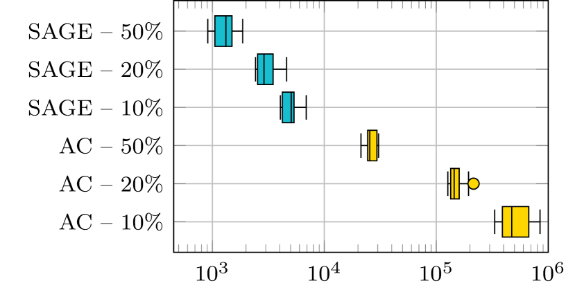
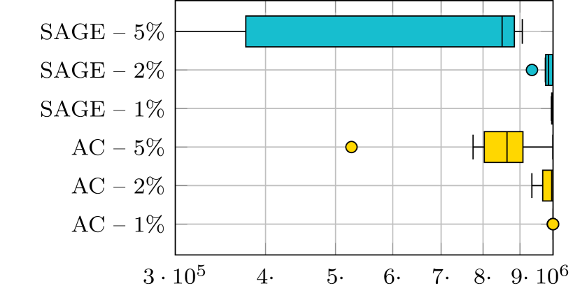
(a) Box plots of convergence times.

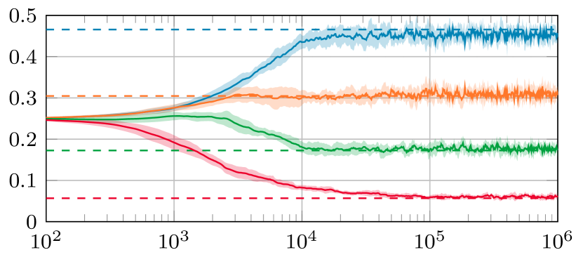
(b) Assignment probabilities under SAGE.

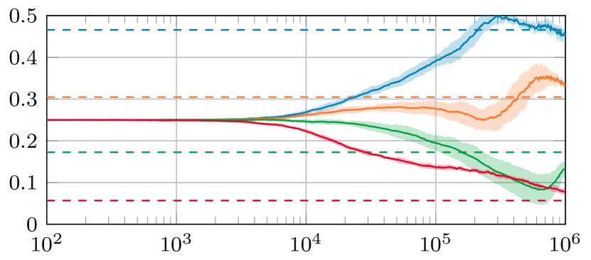
(c) Assignment probabilities under actor-critic.

Figure 1: Performance of SAGE and actor-critic in the load-balancing system. The x-axis is time in logarithmic scale. Figure 1(a) shows the $\epsilon$-convergence times, for $\epsilon\in\{50\%,$ $20\%,$ $10\%,$ $5\%,$ $2\%,$ $1\%\}$. In Figures 1(b) and 1(c), the dashed lines show the optimal assignment probabilities, the solid lines the assignment probabilities under the corresponding algorithm, averaged over 10 independent simulations, and the semitransparent areas the standard deviation; the indices of servers are increasing from top to bottom.

Using Section B.1, we can verify numerically that the admission probability is maximized by $\theta^{\star}\in\mathbb{R}^{4}$ so that $\pi(\theta^{\star})$ $\simeq(0.466,$ $0.3048,$ $0.1724,$ $0.0568)$, yielding admission probability $J(\theta^{\star})\simeq 0.907$. The initial policy $\pi(\Theta_{0})$ is uniform.

Figure 1(a) shows the empirical distribution of the $\epsilon$-convergence time for $\epsilon\in\{50\%,$ $20\%,$ $10\%,$ $5\%,$ $2\%,$ $1\%\}$. Figures 1(b) and 1(c) show the sample trajectories of the assignment probabilities $\pi_{i}(\Theta_{t})$ under SAGE and actor-critic, for $t\in\{10^{2},\ldots,10^{6}\}$ and $i\in\{1,2,3,4\}$. In this example, SAGE converges about 10 times faster than actor-critic, despite both algorithms applying the same gradient step sizes. We believe this is due to the fact that SAGE can “by-design” exploit information on the stationary distribution, which actor-critic cannot. More precisely, referring back to Theorem 1, $\mathrm{D}\log\rho(\theta)$, $\mathrm{Cov}\mathopen{}\mathclose{{}\left[R,x(S)}\right]$, and $\mathbb{E}\mathopen{}\mathclose{{}\left[R\,\nabla\log\pi(A|S,\theta)}\right]$ have dimensions $n\times n$, $n$, and $n$, respectively, where $n=4$ is the number of servers; in contrast, the number of values to be estimated by actor-critic is equal to the number of states in the system, which is of order $c^{n}$, with here $c=10$ and $n=4$.

Numerical results: Impact of the step and batch sizes and memory factor.

Figure 2 shows the same results as Figure 1(b), except that we use step and batch sizes that are consistent with the convergence result of Section 5, as described in the legend of Figure 2. Compared to Figure 1(b), the variance decreases with time at the cost of a slower convergence.

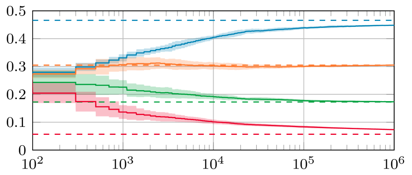
Figure 2: The counterpart of Figure 1(b) when applying SAGE with the step and batchsizes from (16): memory factor $\nu=0$, step sizes $\alpha_{m}=1/(m+1)^{\sigma}$, and batch sizes $t_{m+1}-t_{m}=100(m+1)^{\frac{\sigma}{2}}$, with $\sigma=\frac{2}{3}+\frac{1}{10}$.

6.2 Admission control in an M/M/1 queue

Consider a single-server queue where customers arrive according to a Poisson process with rate $\lambda>0$ and service times are independent and exponentially distributed with rate $\mu>0$. When a customer arrives, the agent makes the decision to either admit or reject it. In the former case, the customer is added to the queue; in the latter case, it is permanently lost. The agent receives a one-time reward $\gamma$ for each accepted customer and incurs a holding cost $\eta$ per customer per time unit, for some $\gamma,\eta>0$. Customers are scheduled according to an arbitrary nonidling nonanticipating policy. The problem is cast to the framework of Section 3 as follows. For each $t\in\mathbb{N}$, let $S_{t}$ denote the number of customers in the system right before the arrival of the $(t+1)$-th customer and $A_{t}$ the decision of admitting or rejecting this customer. We have $\mathcal{S}=\mathbb{N}$ and $\mathcal{A}=\{\textrm{admit},\textrm{reject}\}$. Let $(\Sigma_{\tau},\tau\in\mathbb{R}_{\geq 0})$ denote the continuous-time process that describes the evolution of the number of customers over time and $(T_{t},t\in\mathbb{N})$ the sequence of customer arrival times, so that $S_{0}=\Sigma_{0}$ and $S_{t}=\lim_{\sigma\uparrow T_{t}}\Sigma_{\tau}$ for each $t\in\mathbb{N}_{+}$. Rewards are given by

$$R_{t+1} =r_{\textrm{disc}}(S_{t},A_{t})+\int_{T_{t}}^{T_{t+1}}r_{\textrm{cont}}(\Sigma_{\tau})\mathrm{d}\tau,$$

where $r_{\textrm{disc}}(s,a)=\gamma\mathds{1}[a=\textrm{admit}]$ represents the one-time admission reward and $r_{\textrm{cont}}(s)=-\eta s$ the holding cost incurred continuously over time. We use this commonly used reward in this example but we remark that arbitrary reward functions are also possible.

Policy parametrization and product-form.

Consider the following random policy with threshold $k\in\mathbb{N}$ and parameter $\theta=(\theta_{0},\theta_{1},\ldots,\theta_{k})\in\mathbb{R}^{k+1}$. An incoming customer finding $s$ customers in the system is accepted with probability $\pi(\textrm{admit}|s,\theta)=\pi_{\min(s,k)}(\theta)$ and rejected with probability $\pi(\textrm{reject}|s,\theta)=1-\pi_{\min(s,k)}(\theta)$, where

$$\pi_{i}(\theta)=\frac{1}{1+\mathrm{e}^{-\theta_{i}}},\quad i\in\{0,1,\ldots,k\}.$$ (41)

Taking $k=0$ yields a static random policy, while letting $k$ tend to $+\infty$ yields a fully state-dependent random policy. Assumptions 1, 2 and 3 are satisfied with $n=d=k+1$, $\Omega=\{\theta\in\mathbb{R}^{k+1}:\pi_{k}(\theta)<\frac{\mu}{\lambda}\}$, $\Phi(s)=1$ for each $s\in\mathcal{S}$, $x_{i}(s)=1_{\{s\geq i+1\}}$ for each $i\in\{0,1,\ldots,k-1\}$ and $x_{k}(s)=\max(s-k,0)$, and $\rho_{i}(\theta)=\frac{\lambda}{\mu}\pi_{i}(\theta)$ for each $i\in\{0,1,\ldots,k\}$. It follows that $\nabla\log\rho_{i}=\nabla\log\pi_{i}$ for each $i\in\{0,1,\ldots,k\}$. We have not proved that all assumptions of Section 5 are verified, especially Assumption 7. See Section B.2 for more details on these derivations.

Numerical results with a stable queue.

We compare SAGE and actor-critic in a system with parameters $\lambda=0.7$, $\mu=1$, $\gamma=5$, $\eta=1$, and a threshold-based policy with $k=3$. We have in particular $\Omega=\mathbb{R}^{k+1}$ since $\lambda<\mu$. Using Section B.2, we can verify that the average reward rate is maximized by $\theta^{\star}_{0}=\theta^{\star}_{1}=\theta^{\star}_{2}=-\infty$ and $\theta^{\star}_{3}=+\infty$ (corresponding to the deterministic policy $\pi_{0}(\theta^{\star})$ $=\pi_{1}(\theta^{\star})$ $=\pi_{2}(\theta^{\star})=1$ and $\pi_{3}(\theta^{\star})=0$). Finite maxima could be ensured by adding a regularization term, as Proposition 2 shows. The initial policy is given by $\pi_{i}(\Theta_{0})=\frac{1}{2}$ for each $i\in\{0,1,2,3\}$.

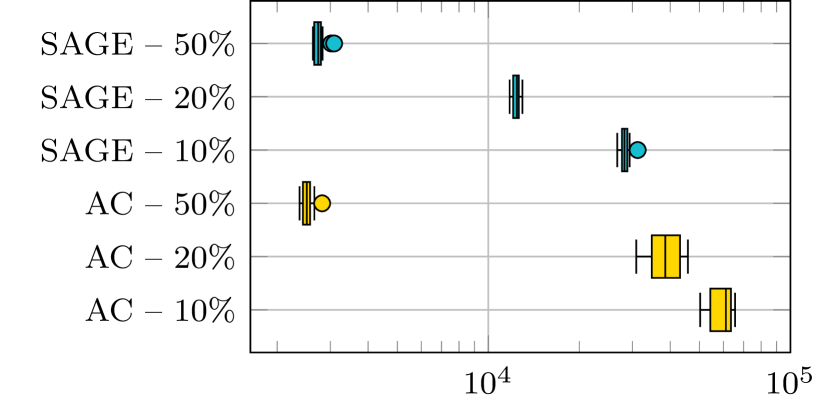
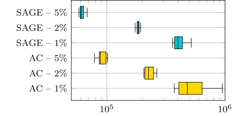
(a) Box plots of convergence times.

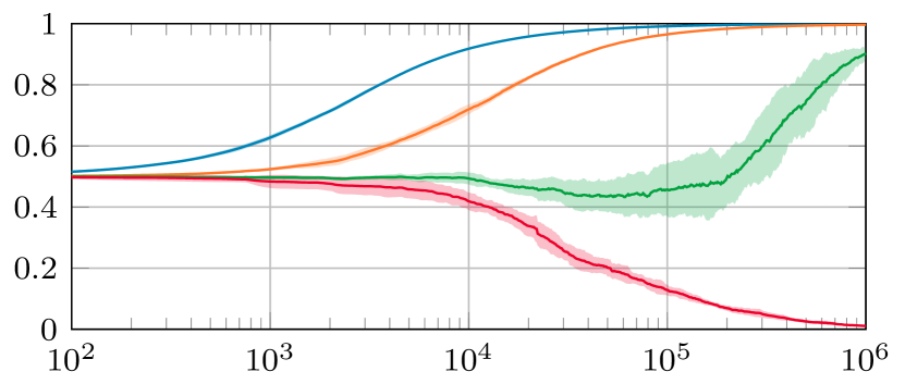
(b) Admission probabilities under SAGE.

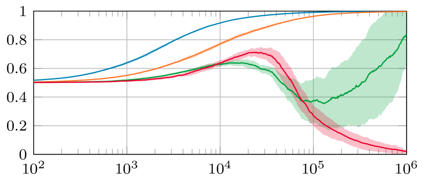
(c) Admission probabilities under actor-critic.

Figure 3: Performance of SAGE and actor-critic in the stable M/M/1 queue with admission control. The legend is similar to Figure 1, except that in Figures 3(b) and 3(c) the solid lines represent assignment probabilities and are ordered in increasing index from top to bottom.

Figure 3(a) shows the empirical distribution of the $\epsilon$-convergence time, for $\epsilon\in\{50\%,$ $20\%,$ $10\%,$ $5\%,$ $2\%,$ $1\%\}$. Figures 3(b) and 3(c) show the sample trajectories of the admission probabilities $\pi_{i}(\Theta_{t})$ under SAGE and actor-critic, for $t\in\{10^{2},\ldots,10^{6}\}$ and $i\in\{0,1,2,3\}$. We observe on Figure 3(a) that the $50\%$-convergence time of actor-critic is slightly lower than that of SAGE, which we explain by the observation that, according to Figures 3(b) and 3(c), the admission probability $\pi_{1}$ converges slightly faster to $\pi_{1}(\theta^{\star})=1$ under actor-critic than under SAGE. On the contrary, the $\epsilon$-convergence time of SAGE is lower than that of actor-critic for $\epsilon\in\{20\%,$ $10\%,$ $5\%,$ $2\%,$ $1\%\}$. That seems to follow from the fact that, under actor-critic, the admission probability $\pi_{3}$ first increases before converging to $\pi_{3}(\theta^{\star})=0$, and the probability $\pi_{2}$ also oscillates before converging to $\pi_{2}(\theta^{\star})=1$. We conjecture this is partly due to the fact that the policy’s structure (constant beyond state 3) cannot be exploited when estimating the state-value function, which slows-down convergence.

Numerical results in a possibly-unstable queue.

We consider the same parameters as before, except that $\lambda=1.4>1=\mu$. The system is stable under the initial policy, again given by $\pi_{i}(\Theta_{0})=\frac{1}{2}$ for each $i\in\{0,1,2,3\}$, but it becomes unstable (in the sense that the underlying Markov chain is transient) if $\pi_{3}(\theta)$ exceeds $\frac{\mu}{\lambda}\simeq 0.714$. Again using the calculations of Section B.2, we can verify that the average reward rate is maximized by choosing $\theta^{\star}_{0}=\theta^{\star}_{1}=+\infty$ and $\theta^{\star}_{2}=\theta^{\star}_{3}=-\infty$ (corresponding to the stable deterministic policy with $\pi_{0}(\theta^{\star})=\pi_{1}(\theta^{\star})=1$ and $\pi_{2}(\theta^{\star})=\pi_{3}(\theta^{\star})=0$). This is an example where convergence can only be guaranteed locally, as not all policies are stable.

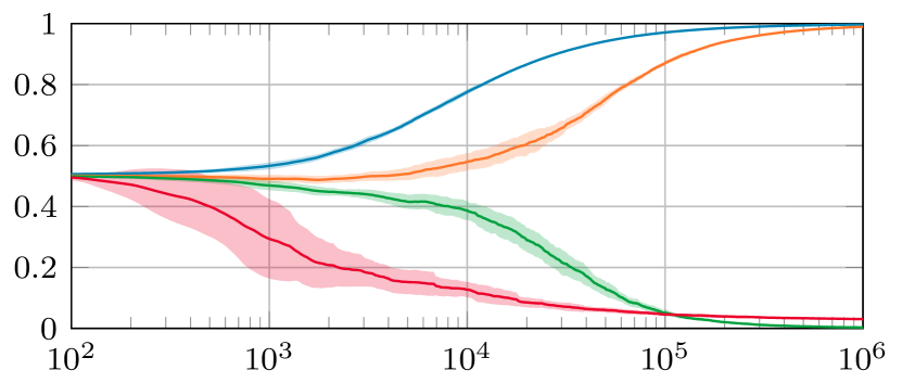
(a) Assignment probabilities under SAGE.

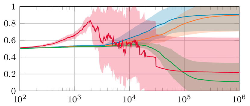
(b) Assignment probabilities under actor-critic.

Figure 4: Performance of SAGE and actor-critic in the possibly-unstable M/M/1 queue with admission control.

Figure 4 is the analog of Figures 3(b) and 3(c) for this possibly-unstable case. The main take-away of Figure 4(a) is that the SAGE-based algorithm converges to a close-to-optimal policy, and that the convergence is actually faster than in the stable case. The SAGE-based algorithm learns first the admission probability $\pi_{3}$ in state 3 or above around $10^{3}$ steps (instead of $10^{5}$ in Figure 3(b)), and then the probabilities $\pi_{0}$, $\pi_{1}$, $\pi_{2}$ around $10^{4}$ steps. We also observe that the admission probability $\pi_{3}$ never reaches zero, which is not an issue since states 3 or above stop being visited once the admission probability $\pi_{2}$ has converged to zero. As suggested by the term $O(\alpha^{2}/\ell)$ in Theorem 2, the chance of reaching unstable policies can be reduced by decreasing the variance of the update $\alpha_{m}H_{m}$. On the contrary, Figure 4(b) suggests that actor-critic has more difficulties in coping with instability in this example. Sample trajectories of actor-critic in Section B.3 give additional information: convergence towards the optimal policy is observed in 8 out of 10 trajectories, but in all trajectories we observe a transitory regime where the admission probability $\pi_{3}$ fluctuates rapidly.

Appendix A Actor-critic algorithm

The actor-critic algorithm is first mentioned in Section 3.4 and compared to our SAGE-based policy-gradient algorithm in Section 6. We focus on the version of the actor-critic algorithm described in [31, Section 13.6] for the average-reward criterion in infinite horizon. The algorithm relies on the following expression for $\nabla J(\theta)$, which is a variant of the policy-gradient theorem [31, Chapter 13]:

$$\nabla J(\theta) \propto\mathbb{E}\mathopen{}\mathclose{{}\left[\mathopen{}\mathclose{{}\left(R-J(\theta)+v(S^{\prime})-v(S)}\right)\nabla\log\pi(A|S,\theta)}\right],$$

where $(S,A,R,S^{\prime})$ is a quadruplet of random variables such that $S\sim p(\,\cdot\,|\theta)$, $A|S\sim\pi(\,\cdot\,|S,\theta)$, and $(R,S^{\prime})|(S,A)\sim P(\,\cdot\,,\,\cdot\,|S,A)$ (so that in particular $(S,A,R)\sim$ stat($\theta$)), and $v$ is the state-value function.

The pseudocode of the procedure Gradient used in the actor-critic algorithm is given in Algorithm 3. This procedure is to be implemented within Algorithm 1 with batch sizes equal to one, meaning that $t_{m+1}=t_{m}+1$ for each $m\in\mathbb{N}$. We assume to simplify notation that all variables from Algorithm 1 are accessible inside Algorithm 3. The variable $\overline{R}$ updated on 6 is a biased estimate of $J(\Theta_{m})$, while the table $V$ updated on 7 is a biased estimator of the state-value function under policy $\pi(\Theta_{m})$. Compared to [31, Section 13.6], the value function is encoded by a table $V$ and there are no eligibility traces. If the state space $\mathcal{S}$ is infinite, the table $V$ is initialized at zero over a subset of $\mathcal{S}$ containing the initial state $S_{0}$ and expanded with zero padding whenever necessary.

Algorithm 3 Actor-critic algorithm [31, Section 13.6] to be called on 9 of Algorithm 1, with batch sizes equal to one.

1:Input: Positive and differentiable policy parametrization $(s,\theta,a)\mapsto\pi(a|s,\theta)$

2:Parameters: Step sizes $\alpha_{\overline{R}}>0$ and $\alpha_{v}>0$

3:Initialization: $\bullet$ $\overline{R}\leftarrow 0$ $\bullet$ $V[s]\leftarrow 0$ for each $s\in\mathcal{S}$

4:procedure Gradient($t$)

5:     $\delta\leftarrow R_{t+1}-\overline{R}+V[S_{t+1}]-V[S_{t}]$

6:     Update $\overline{R}\leftarrow\overline{R}+\alpha_{\overline{R}}\delta$

7:     Update $V[S_{t}]\leftarrow V[S_{t}]+\alpha_{v}\delta$

8:     return $\delta\,\nabla\log\pi(A_{t}|S_{t},\Theta_{t})$

9:end procedure

Appendix B Examples

This appendix provides detailed calculations for the examples of Section 6. We first consider the load-balancing example of Section 6.1, and then we move to the M/M/1 queue with admission control of Section 6.2. For simplicity, we decided to focus on systems where decisions are made upon arrivals of customers (jobs, items, etc.), so that the arrival times of customers are natural discretization times. Incoming customers arrive according to Poisson processes so that, by the PASTA property [34], the stochastic processes obtained by observing the system state either at arrival times or continuously over time have the same stationary distribution.

B.1 Load-balancing system

We first consider the load-balancing example of Section 6.1. Recall that customers arrive according to a Poisson process with rate $\lambda>0$, there are $n$ servers at which service times are distributed exponentially with rates $\mu_{1}$, $\mu_{2}$, $\ldots$, $\mu_{n}$, respectively, and the system can contain at most $c$ customers, for some $c\in\mathbb{N}_{+}$. The agent’s goal is to choose a static random policy that maximizes the admission probability. We first verify that the system satisfies Assumptions 1, 2 and 3, then we provide an algorithm to evaluate the objective function when the parameters are known; this is used in particular for performance comparison with the optimal policy in the numerical results. Lastly, we discuss the assumptions of Section 5. Throughout this section, we assume that we apply the policy $\pi(\theta)$ defined by (40) for some parameter $\theta\in\mathbb{R}^{n}$.

Product-form stationary distribution.

That Assumption 1 is satisfied follows from the facts that the rates and probabilities $\lambda$, $\mu_{1}$, $\mu_{2}$, $\ldots$, $\mu_{n}$ $\pi_{1}(\theta)$, $\pi_{2}(\theta)$, $\ldots$, $\pi_{n}(\theta)$ are positive, and that the state space $\mathcal{S}$ is finite. Assumption 2 is satisfied because the state space is finite. This system can be modeled either as a loss Jackson network with $n$ queues (one queue for each server in the load-balancing system) or as a closed Jackson network with $n+1$ queues (one queue for each server in the system, plus another signaling available positions in the system, with service rate $\lambda$). Either way, we can verify (for instance by writing the balance equations) that the stationary distribution of the continuous-time Markov chain that describes the evolution of the system state is given by:

$$p(s|\theta) =\frac{1}{Z(\theta)}\prod_{i=1}^{n}\mathopen{}\mathclose{{}\left(\frac{\lambda}{\mu_{i}}\pi_{i}(\theta)}\right)^{s_{i}},\quad s=(s_{1},s_{2},\ldots,s_{n})\in\mathcal{S},$$ (42)

where $Z(\theta)$ follows by normalization. This is exactly (9–PF) from Assumption 3, with $n=d$, $\Omega=\mathbb{R}^{n}$, $\Phi(s)=1$ for each $s\in\mathcal{S}$, $x_{i}(s)=s_{i}$ for each $i\in\{1,2,\ldots,n\}$ and $s\in\mathcal{S}$, and $\rho_{i}(\theta)=\frac{\lambda}{\mu_{i}}\pi_{i}(\theta)$ for each $i\in\{1,2,\ldots,n\}$. The function $\rho$ defined in this way is differentiable. Assumption 3 is therefore satisfied, as the distribution of the system seen at arrival times is also (42) according to the PASTA property. Besides the sufficient statistics $x$, the inputs of Algorithm 2 are $\nabla\log\pi(a|s,\theta)=\mathds{1}_{a}-\pi(\theta)$, where $\mathds{1}_{a}$ is the $n$-dimensional vector with one in component $a$ and zero elsewhere, and $\pi(\theta)$ is the policy seen as a (column) vector, and $\mathrm{D}\log\rho(\theta)=\textrm{Id}-\mathds{1}\pi(\theta)^{\intercal}$, where Id is the $n$-dimensional identity matrix, $\mathds{1}$ is the $n$-dimensional vector with all-one components, and $\pi(\theta)^{\intercal}$ is the (row) vector obtained by transposing $\pi(\theta)$. This latter equation can be used to verify Assumption 5.

Objective function.

When all system parameters are known, the normalizing constant $Z(\theta)$ and admission probability $J(\theta)$ can be calculated efficiently using a variant of Buzen’s algorithm [7] for loss networks. Let us first define the array $G=(G_{\underline{c},\underline{n}})_{\underline{c}\in\{0,1,\ldots,c\},\underline{n}\in\{1,2,\ldots,n\}}$ by

$$G_{\underline{c},\underline{n}} =\sum_{\begin{subarray}{c}s\in\mathbb{N}^{\underline{n}}:\\ |s|\leq\underline{c}\end{subarray}}\prod_{i=1}^{\underline{n}}{\rho_{i}(\theta)}^{s_{i}},\quad\underline{c}\in\{0,1,\ldots,c\},\quad\underline{n}\in\{1,2,\ldots,n\}.$$

The dependency of $G$ on $\theta$ is left implicit to alleviate notation. The normalizing constant and admission probability are given by $Z(\theta)=G_{c,n}$ and $J(\theta)=G_{c-1,n}/G_{c,n}$, respectively. Defining the array $G$ allows us to calculate these metrics more efficiently than by direct calculation, as we have $G_{0,\underline{n}}=1$ for each $\underline{n}\in\{1,2,\ldots,n\}$, and

$$G_{\underline{c},1} =1+{\rho_{i}(\theta)}{G_{\underline{c}-1,1}}, \underline{c}\in\{1,2,\ldots,c\},$$

$$G_{\underline{c},\underline{n}} =G_{\underline{c},\underline{n}-1}+{\rho_{i}(\theta)}G_{\underline{c}-1,\underline{n}}, \underline{c}\in\{1,2,\ldots,c\},\quad\underline{n}\in\{2,3,\ldots n\}.$$

Assumptions of Section 5.

Assumptions 4, 5, and 6 are automatically satisfied because the state space is finite (with $|\mathcal{S}|=c$). Verifying Assumption 7 is challenging since it requires computing $\mathrm{Hess}_{\theta^{\star}}J$ at the maximizer $\theta^{\star}$, which depends in an implicit manner on the parameters of the system such as the arrival rate $\lambda$, service rates $\mu_{1},\mu_{2},\ldots,\mu_{n}$, and policy $\pi(\theta^{\star})$. However, the nondegeneracy property of the Hessian for smooth functions is a property that is commonly stable in the following sense: if a function satisfies this property, then it will still be satisfied after any small-enough smooth perturbation. In particular, smooth functions with isolated nondegenerate critical points—also known as Morse functions—are dense and form an open subset in the space of smooth functions; see [25, Section 1.2]. Thus, unless the example is adversarial or presents symmetries, we can expect Assumption 7 to hold.

B.2 M/M/1 queue with admission control

We now consider the example of Section 6.2. Recall that customers arrive according to a Poisson process with rate $\lambda>0$ and service times are exponentially distributed with rate $\mu>0$. The reward rate is equal to the difference between an admission reward proportional to the admission probability and a holding cost proportional to the mean queue size. As in Section B.1, we first verify that Assumptions 1, 2 and 3 are satisfied, then we give a closed-form expression for the objective function, and lastly we discuss the assumptions of Section 5. We consider a random threshold-based policy of the form (41) for some parameter $\theta\in\Omega$, where $\Omega=\{\theta\in\mathbb{R}^{k+1}:\pi_{k}(\theta)<\frac{\mu}{\lambda}\}$.

Product-form stationary distribution.

The evolution of the number of customers in the queue defines a birth-and-death process with birth rate $\lambda\pi_{\min(s,k)}(\theta)$ and death rate $\mu\mathds{1}[s\geq 1]$ in state $s$, for each $s\in\{0,1,2,\ldots\}$. This birth-and-death process is irreducible because these rates are positive, and it is positive recurrent because $\lambda\pi_{k}(\theta)<\mu$ by definition of $\Omega$. This verifies Assumption 1. The stationary distribution is given by

$$p(s) =\frac{1}{Z(\theta)}\prod_{q=0}^{s-1}\frac{\lambda}{\mu}\pi(\textrm{admit}|q,\theta)=\frac{1}{Z(\theta)}\mathopen{}\mathclose{{}\left[\prod_{i=0}^{k-1}\mathopen{}\mathclose{{}\left(\frac{\lambda}{\mu}\pi_{i}(\theta)}\right)^{\mathds{1}[s\geq i+1]}}\right]\mathopen{}\mathclose{{}\left(\frac{\lambda}{\mu}\pi_{k}(\theta)}\right)^{\max(s-k,0)},\quad s\in\mathbb{N},$$ (43)

where the second equality follows by injecting (41), and the value of $Z(\theta)$ follows by normalization. We recognize (9–PF) from Assumption 3, with $n=d=k+1$, $\Phi(s)=1$ for each $s\in\mathcal{S}$, $x_{i}(s)=1_{\{s\geq i+1\}}$ for each $i\in\{0,1,\ldots,k-1\}$ and $x_{k}(s)=\max(s-k,0)$ for each $s\in\mathcal{S}$, and $\rho_{i}(\theta)=\frac{\lambda}{\mu}\pi_{i}(\theta)$ for each $i\in\{0,1,\ldots,k\}$. The function $\rho$ defined in this way is differentiable. Assumption 3 is therefore satisfied, as the distribution of the system seen at arrival times is also (43) according to the PASTA property. For each $a\in\{\textrm{admit},\textrm{reject}\}$ and $s\in\mathbb{N}$, $\nabla\log\pi(a|s,\theta)$ is the $(k+1)$-dimensional column vector with value $\mathds{1}[a\,=\,\textrm{admit}]-\pi_{i}(\theta)$ in component $i=\min(s,k)$ and zero elsewhere, and $\mathrm{D}\log\rho(\theta)$ is the $(k+1)$-dimensional diagonal matrix with diagonal coefficient $1-\pi_{i}(\theta)$ in position $i$, for each $i\in\{0,1,\ldots,k\}$. This can be used to verify that Assumption 5 is satisfied.

Objective function.

The objective function is given by $J(\theta)=\gamma\mathbb{P}\mathopen{}\mathclose{{}\left[A=\textrm{admit}}\right]-\frac{\eta}{\lambda}\mathbb{E}\mathopen{}\mathclose{{}\left[S}\right]$, where

$$\mathbb{P}\mathopen{}\mathclose{{}\left[A=\textrm{admit}}\right] =\sum_{i=0}^{k-1}p(i|\theta)\pi_{i}(\theta)+\Bigl{(}1-\sum_{i=0}^{k-1}p(i|\theta)\Bigr{)}\pi_{k}(\theta),$$

$$\mathbb{E}\mathopen{}\mathclose{{}\left[S}\right] =\sum_{i=0}^{k-1}ip(i|\theta)+\frac{p(k|\theta)}{1-\rho_{k}(\theta)}\Bigl{(}k+\frac{\rho_{k}(\theta)}{1-\rho_{k}(\theta)}\Bigr{)},$$

$$Z(\theta) =\sum_{s=0}^{k-1}\Bigl{(}\prod_{i=0}^{s-1}\rho_{i}(\theta)\Bigr{)}+\Bigl{(}\prod_{i=0}^{k-1}\rho_{i}(\theta)\Bigr{)}\frac{1}{1-\rho_{k}(\theta)},$$

with the convention that empty sums are equal to zero and empty products are equal to one. All calculations remain valid in the limit as $\pi_{i}(\theta)\to 1$ for some $i\in\{0,1,\ldots,k\}$ (corresponding to $\theta_{i}\to+\infty$). In the limit as $\pi_{i}(\theta)\to 0$ for some $i\in\{0,1,\ldots,k\}$, we can study the restriction of the birth-and-death process to the state space $\{0,1,\ldots,\underline{c}\}$, where $\underline{c}=\min\{i\in\{0,1,\ldots,k\}:\pi_{i}(\theta)=0\}$.

Assumptions of Section 5.

For any closed set $U\subset\Omega$, it can be shown that there exists a Lyapunov function $\mathcal{L}$ uniformly over $\theta\in U$ such that $\mathcal{L}(s,a)=\exp(cs)$ for some $c>0$, depending on $U$ and the model parameters. Hence, Assumptions 4, 5 and 6 are satisfied. In general, Assumption 7 does not hold for this example because maxima occur only as $|\theta|\to\infty$. As suggested by Proposition 2, by adding a small regularization term, we can guarantee Assumption 7 while simultaneously ensuring that the maximizer is bounded. In practice, using a regularization term can additionally present some benefits such as avoiding vanishing gradients and saddle points.

B.3 Example trajectories of the actor-critic algorithm in the M/M/1 unstable queue

In the second set of experiments of Section 6.2, SAGE and actor-critic are applied to optimize the admission probability in an M/M/1 queue with parameters $\lambda=1.6$, $\mu=1$, $\gamma=1$, and $\eta=5$. With our parameterizations of the policies in (41) with $k=3$, the policy is stable if and only if $\pi_{3}(\theta)<\frac{\mu}{\lambda}\simeq 0.714$, so that in particular the initial policy $\pi(\Theta_{0})=(\frac{1}{2},\frac{1}{2},\frac{1}{2},\frac{1}{2})$ is stable. As observed in Figure 4(b), the actor-critic algorithm seems to exhibit poor convergence properties in this example. Figure 5 supplements this observation by plotting four sample trajectories based on which the mean and standard deviations in Figure 4(b) were computed. The first three plots show trajectories where actor-critic seems to eventually converge to the optimal, while the last plot shows one of the two trajectories where convergence to the optimal policy is not observed. In either case, we observe a first transitory period where the admission probability in state 3 or above varies very rapidly before eventually stabilizing around either 0 (its optimal value) or 1.

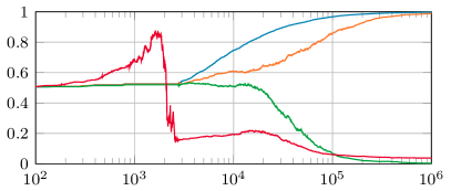
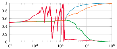
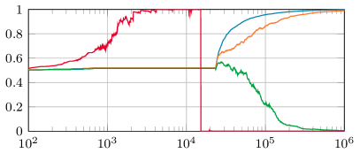
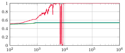
Figure 5: Example assignment probabilities under actor-critic.

Appendix C Proof of Theorem 2

C.1 Preliminaries

We are going to use concentration inequalities for Markov chains. Such results are common in the literature (for example, see [17]), and will be required to get a concentration bound of the plug-in estimators from (15).

Denote by $B_{\epsilon}(\theta)$ the open ball of radius $\epsilon$ centered at $\theta\in\Omega\subseteq\mathbb{R}^{n}$ and $\mathcal{Y}=\mathcal{S}\times\mathcal{A}$. Given a function $q:\mathcal{Y}\to\mathbb{R}$ and the Lyapunov function $\mathcal{L}:\mathcal{Y}\to[1,\infty)$ from Assumption 4, define

$$|q|_{\mathcal{L}}=\sup_{y\in\mathcal{Y}}\frac{|q(y)|}{\mathcal{L}(y)}.$$ (44)

Given a signed measure $\nu$, we also define the seminorm

$$|\nu|_{\mathcal{L}}=\sup_{|q|_{\mathcal{L}}\leq 1}|\nu[q]|=\sup_{|q|_{\mathcal{L}}\leq 1}\Bigl{|}\int q(y)\nu(dy)\Bigr{|}.$$ (45)

Equations 44 to 45 imply that

$$|\nu[q]|\leq|\nu|_{\mathcal{L}}|q|_{\mathcal{L}}.$$ (46)

Note that we defined $|\cdot|_{\mathcal{L}}$ for a unidimensional function. Given instead $m$ functions $q_{i}:\mathcal{Y}\to\mathbb{R}$, for the higher-dimensional function $q:\mathcal{Y}\to\mathbb{R}^{m}$ that satisfies for all $y\in\mathcal{Y}$, $q(y)=(q_{1}(y),\ldots,q_{l}(y))$, we define $|q|_{\mathcal{L}}=\sqrt{\sum_{i=1}^{l}|q_{i}|_{\mathcal{L}}^{2}}$.

The following lemma yields the concentration inequalities required:

Lemma 5.

Let $\{Y_{n}\}_{n\geq 1}$ be a geometrically ergodic Markov chain with invariant distribution $p$ and transition matrix $P(\,\cdot\,,\,\cdot\,)$. Let the Lyapunov function be $\mathcal{L}:\mathcal{Y}\to\mathbb{R}$. From geometric ergodicity, there exists $C>0$ and $\lambda\in(0,1)$ such that for any $y\in\mathcal{Y}$,

$$|P^{m}(\,\cdot\,|y)-p(\cdot)|_{\mathcal{L}}\leq C\lambda^{m}.$$ (47)

Let $\mathcal{F}=\sigma(Y_{1})$ be the $\sigma$-algebra of $Y_{1}$. Let $q:\mathcal{Y}\to\mathbb{R}^{m}$ be a measurable function such that $|q|_{\mathcal{L}}<\infty$. For a finite trajectory $Y_{1},\ldots,Y_{M}$ of the Markov chain, we define the empirical estimator for $p[q]$ as

$$\hat{p}_{M}[q]=\frac{1}{M}\sum_{i=1}^{M}q(Y_{i}).$$ (48)

With these assumptions, there exists $C^{\prime}$ depending on $C$ and $\lambda$ such that

$$\Bigl{|}\mathbb{E}\Bigl{[}p[q]-\hat{p}_{M}[q]\big{|}\mathcal{F}\Bigr{]}\Bigr{|}\leq\frac{C^{\prime}|q|_{\mathcal{L}}}{M}\mathcal{L}(Y_{1}),$$ (49)

and for $l\in\{1,2,4\}$,

$$\mathbb{E}\Bigl{[}|p[q]-\hat{p}_{M}[q]|^{l}\big{|}\mathcal{F}\Bigr{]}\leq\frac{C^{\prime}|q|_{\mathcal{L}}^{l}}{M^{l/2}}\mathcal{L}^{l}(Y_{1}).$$ (50)

Proof.

We refer to [14, Prop. 12] for a proof of (50). What remains is to prove (49).

Observe that for $y\in\mathcal{Y}$, $P(y)=P(\,\cdot\,|y)$ is a distribution over $\mathcal{Y}$. Conditional on $\mathcal{F}$, there exists $C>0$ such that

$$\Bigl{|}\mathbb{E}\Bigl{[}\frac{1}{M}\sum_{i=1}^{M}q(Y_{i})-p[q]\Big{|}\mathcal{F}\Bigr{]}\Bigr{|} \leq\frac{1}{M}\sum_{i=1}^{M}\bigl{|}P^{i}(Y_{1})[q]-p[q]\bigr{|}=\frac{1}{M}\sum_{i=1}^{M}\bigl{|}\bigl{(}P^{i}(Y_{1})-p\bigr{)}[q]\bigr{|}$$

$$\leq\frac{1}{M}\sum_{i=1}^{M}\bigl{|}P^{i}(\,\cdot\,|Y_{1})-p(\cdot)\bigr{|}_{\mathcal{L}}|q|_{\mathcal{L}}\mathcal{L}(Y_{1})\leq\frac{|q|_{\mathcal{L}}}{M}\sum_{i=1}^{M}C\lambda^{i}\mathcal{L}(Y_{1})$$

$$\leq\frac{C|q|_{\mathcal{L}}}{M(1-\lambda)}\mathcal{L}(Y_{1}).$$ (51)

This concludes the proof. ∎

In epoch $m$, the Markov chain $\{S_{t}\}_{t\in[t_{m},t_{m+1}]}$ with control parameter $\Theta_{m}$ has a Lyapunov function $\mathcal{L}_{v}$. Intuitively, as a consequence of Assumption 4, we can show that the process does not drift to infinity on the event $\mathcal{B}_{m}$ (despite the changing control parameter $\Theta_{m}$).

Specifically, for $m>0$, let $\{S_{t}\}_{i\in[t_{m},t_{m+1}]}$ be the Markov chain trajectory with transition probabilities $P(\Theta_{m})$, where $\Theta_{m}$ is given by the updates in (3) and (15) and initial state $S_{0}\in\mathcal{S}$. Recall that $\mathcal{B}_{m}$ is defined in (28). We can then prove the following:

Lemma 6.

Suppose Assumption 4 holds. There exists $D<\infty$ such that for $m>0$, ${\mathbb{E}}\bigl{[}\mathcal{L}_{v}(S_{t_{m+1}})\allowbreak\mathds{1}[\mathcal{B}_{m}]\bigr{]}<D$.

Proof.

We will give an inductive argument. A similar argument can be found in [3].

First, observe that for $m=0$, $S_{0}$ is fixed. There thus exists a $D$ such that $\mathcal{L}_{v}(S_{0})<D$.

Next, assume that ${\mathbb{E}}[\mathcal{L}_{v}(S_{t_{m}})\mathds{1}[\mathcal{B}_{m-1}]]<D$. On the event $\mathcal{B}_{m}$, Assumption 4 holds since $\Theta_{1},\ldots,\Theta_{m-1},\Theta_{m}\in V_{\mathfrak{r},\delta}(\theta^{\star})\subset U$. Thus, on the event $\mathcal{B}_{m}$, and when additionally conditioning on $S_{t_{m+1}-1}$ and $\Theta_{m}$, the following holds true:

$${\mathbb{E}}\bigl{[}\mathcal{L}_{v}(S_{t_{m+1}})\mathds{1}[\mathcal{B}_{m}]\bigr{]} \leq{\mathbb{E}}\bigl{[}{\mathbb{E}}[\mathcal{L}_{v}(S_{t_{m+1}})\mathds{1}[\mathcal{B}_{m}]|S_{t_{m+1}-1}]\bigr{]}$$

$$={\mathbb{E}}\bigl{[}\mathds{1}[\mathcal{B}_{m}]P_{\Theta_{m}}\mathcal{L}_{v}(S_{t_{m+1}-1})\bigr{]}$$ (52)

$$\leq{\mathbb{E}}\bigl{[}\mathds{1}[\mathcal{B}_{m}][\lambda\mathcal{L}_{v}(S_{t_{m+1}-1})+b]\bigr{]}.$$

The last step followed from Assumption 4.

Observe finally that the bound in (52) can be iterated by conditioning on $S_{t_{m+1}-2}$; so on and so forth. After $t_{m+1}-t_{m}$ iterations, one obtains

$${\mathbb{E}}\bigl{[}\mathcal{L}_{v}(S_{t_{m+1}})\mathds{1}[\mathcal{B}_{m}]\bigr{]}\leq\lambda{\mathbb{E}}\bigl{[}\mathcal{L}_{v}(S_{t_{m}})\mathds{1}[\mathcal{B}_{m}]\bigr{]}+\frac{b}{1-\lambda}.$$ (53)

Noting that $\mathds{1}[\mathcal{B}_{m}]\leq\mathds{1}[\mathcal{B}_{m-1}]$, the claim follows by induction if we choose $D$ large enough such that $\lambda D+b/(1-\lambda)<D$. ∎

C.2 Proof of Theorem 2

To prove Theorem 2, we more–or–less follow the arguments of [13, Thm. 25]. Modifications are however required because we consider a Markovian setting instead. Specifically, we rely on the bounds in Lemmas 2, 3 and 4 instead of the bounds in [13, Prop. 20, Prop. 21, Prop. 24], respectively.

Let us begin by bounding

$$\mathbb{P}[J^{\star}-J(\Theta_{m})>\epsilon|\mathcal{B}_{0}].$$ (54)

Here, $\mathcal{B}_{0}=\{\Theta_{0}\in V_{\mathfrak{r},\delta}(\theta^{\star})\}$—recall (28). Theorem 2 assumes that we initialize in a set $V$ which we will specify later but satisfies $V\subset V_{\mathfrak{r},\delta}(\theta^{\star})$. Since we can initialize $\Theta_{0}$ with positive probability in $V$, we have that $\mathbb{P}[\mathcal{B}_{0}]\geq\mathbb{P}[\Theta_{0}\in V]>1/c>0$ for some $c>0$. Thus, we will focus on finding an upper bound of

$$\mathbb{P}[J^{\star}-J(\Theta_{m})>\epsilon|\mathcal{B}_{0}]\leq c\mathbb{P}[\{J^{\star}-J(\Theta_{m})>\epsilon\}\cap\mathcal{B}_{0}].$$ (55)

Denote the orthogonal projection of $\Theta_{m}$ onto $\mathcal{M}\cap U$ by $\tilde{\Theta}_{m}=\mathfrak{p}(\Theta_{m})$. We can relate the objective gap $J^{\star}-J(\Theta_{m})$ to the distance $D_{m}:=\mathrm{dist}(\Theta_{m},\mathcal{M}\cap U)$ as follows. Since $J$ is twice continuously differentiable with maximum $J^{\star}$ attained at $\mathcal{M}\cap U$, the function $J(\theta)$ with $\theta\in V_{\mathfrak{r},\delta}(\theta^{\star})$ is locally Lipschitz with constant $\mathfrak{l}_{\mathfrak{r},\delta}(\Theta^{\star})>0$. On the event $\mathcal{B}_{m}$, we have $\Theta_{m}\in V_{\mathfrak{r},\delta}(\theta^{\star})$ and therefore we have the inequality

$$J^{\star}-J(\Theta_{m})=J(\tilde{\Theta}_{m})-J(\Theta_{m})\leq\mathfrak{l}_{\mathfrak{r},\delta}(\theta^{\star})\bigl{|}\tilde{\Theta}_{m}-\Theta_{m}\bigr{|}=\mathfrak{l}_{\mathfrak{r},\delta}(\theta^{\star})D_{m}.$$ (56)

Consequently, we have the bound

$$\mathbb{P}[\{J^{\star}-J(\Theta_{m})>\epsilon\}\cap\mathcal{B}_{m}]\leq\mathbb{P}\Bigl{[}\Bigl{\{}D_{m}\geq\frac{\epsilon}{\mathfrak{l}_{\mathfrak{r},\delta}(\theta^{\star})}\Bigr{\}}\cap\mathcal{B}_{m}\Bigr{]}$$ (57)

If we define $\epsilon^{\prime}=\epsilon/\mathfrak{l}_{\mathfrak{r},\delta}(\theta^{\star})$, the right-hand side of (57) can also be written as

$$\mathbb{P}[\{D_{m}\geq\epsilon^{\prime}\}\cap\mathcal{B}_{m}] =\mathbb{E}[\mathds{1}[D_{m}\geq\epsilon^{\prime}]\mathds{1}[\mathcal{B}_{m}]]$$

$$=\mathbb{E}[\mathds{1}[D_{m}\mathds{1}[B_{m}]\geq\epsilon^{\prime}]]=\mathbb{P}[D_{m}\mathds{1}[B_{m}]\geq\epsilon^{\prime}]$$ (58)

by the positivity of $D_{m}$.

Next, we use (i) the law of total probability noting that $\mathcal{B}_{m}\subset\mathcal{B}_{0}$, (ii) the bound (57) and the inequality $\mathbb{P}[A\cap B]\leq\mathbb{P}[A]$ for any two events $A,B$, and finally, (iii) the equality (58). We obtain

$$\mathbb{P}[\{J^{\star}-J(\Theta_{m})>\epsilon\}\cap\mathcal{B}_{0}] \overset{\textnormal{(i)}}{\leq}\mathbb{P}[\{J^{\star}-J(\Theta_{m}))>\epsilon\}\cap\mathcal{B}_{m}]+\mathbb{P}[\{J^{\star}-J(\Theta_{m}))>\epsilon\}\cap\overline{\mathcal{B}_{m}}]$$

$$\overset{\textnormal{(ii)}}{\leq}\mathbb{P}[\{D_{m}\geq\epsilon^{\prime}\}\cap\mathcal{B}_{m}]+\mathbb{P}[\overline{\mathcal{B}_{m}}]$$

$$\overset{\textnormal{(iii)}}{\leq}\mathbb{P}[D_{m}\mathds{1}[\mathcal{B}_{m}]\geq\epsilon^{\prime}]+\mathbb{P}[\overline{\mathcal{B}_{m}}]$$

$$\leq\mathbb{P}[D_{m}\mathds{1}[\mathcal{B}_{m-1}]\geq\epsilon^{\prime}]+\mathbb{P}[\overline{\mathcal{B}_{m}}]=\textnormal{Term I}+\textnormal{Term II}.$$ (59)

Term I can be bounded by using Markov’s inequality and Lemma 2. This shows that

$$\textnormal{Term I}\leq c\epsilon^{\prime-2}m^{-\sigma-\kappa}.$$ (60)

Term II can be bounded by Lemma 4. Specifically, one finds that there exists a constant $c>0$ such that, if $\Theta_{0}\in V_{\mathfrak{r}/2,\delta}(\Theta^{\star})$,

$$\textnormal{Term II}\leq 1-\mathrm{exp}\Bigl{(}-\frac{c\alpha^{2}}{\delta^{2}\ell}\Bigr{)}+c\delta^{-2}\ell^{-1}m^{1-\sigma-\kappa}+c\alpha\frac{(m^{1-3/2\sigma-\kappa/2}+\ell^{-1/2}m^{1-5\sigma/8-\kappa/2})}{(\mathfrak{r}/2-2\delta)_{+}}.$$ (61)

Note next that for any $\alpha\in(0,\alpha_{0}]$ and $c>0$ there exists $\delta_{0}$ such that for any $\delta\in(0,\delta_{0}]$ there exists $\ell_{0}$ such that if $\ell\in[\ell_{0},\infty)$ there exists a constant $c^{\prime}>0$ such that we have the inequality $1-\exp{(-{c\alpha^{2}}/{\delta^{2}\ell})}\leq c^{\prime}{\alpha^{2}}/{\delta^{2}\ell}$. We can substitute this bound in (62) to yield

$$\textnormal{Term II}\leq c^{\prime}\frac{\alpha^{2}}{\delta^{2}\ell}+\textnormal{\emph{idem}}.$$ (62)

Bounding (59) by the sum of (60) and (62), and substituting the bound in (55) reveals that there exists a constant $c^{\prime\prime}>0$ such that if $\Theta_{0}\in V_{\mathfrak{r}/2,\delta}(\theta^{\star})$ then

$$\mathbb{P}[J^{\star}-J(\Theta_{m})>\epsilon|\mathcal{B}_{0}] \leq c^{\prime\prime}(\epsilon^{\prime})^{-2}m^{-\sigma-\kappa}+c^{\prime\prime}\alpha^{2}\delta^{-2}\ell^{-1}+c^{\prime\prime}\delta^{-2}\ell^{-1}m^{1-\sigma-\kappa}$$

$$\phantom{\leq}+c^{\prime\prime}\alpha\frac{(m^{1-3/2\sigma-\kappa/2}+\ell^{-1/2}m^{1-5\sigma/8-\kappa/2})}{(\mathfrak{r}/2-2\delta)_{+}}.$$ (63)

Note that the exponents of $m$ in (63) satisfy that since $\sigma\in(2/3,1)$, $1-3/2\sigma-\kappa/2\leq-\kappa/2$ as well as $1-5\sigma/8-\kappa/2<1-\sigma/2-\kappa/2$. Finally, let the initialization set be $V=V_{\mathfrak{r}/2,\delta}(\theta^{\star})$. Note that since $\{\Theta_{0}\in V\}\subset\mathcal{B}_{0}$ there exists a constant $c^{\prime\prime\prime}>0$ such that

$$\mathbb{P}[J^{\star}-J(\Theta_{m})>\epsilon|\Theta_{0}\in V]\leq c^{\prime\prime\prime}\mathbb{P}[J^{\star}-J(\Theta_{m})>\epsilon|\mathcal{B}_{0}].$$ (64)

Substituting the upper bound (63) in (64) concludes the proof. $\Box$

C.3 Proof of Lemma 1

For simplicity, we will denote $t_{m+1}-t_{m}=T_{m}$, $X_{t}=x(S_{t})$ throughout this proof. We also temporarily omit the summation indices for the epoch. We note that the policies defined in (5) satisfy that for $(s,a)\in\mathcal{S}\times\mathcal{A}$,

$$\bigl{(}\nabla\log\pi(a|s,\theta)\bigr{)}_{i,a^{\prime}} =\begin{cases}\mathds{1}[a=a^{\prime}]-\pi(a^{\prime}|s,\theta)&\text{if }i=h(s),\\ 0&\text{otherwise}.\end{cases}$$

In particular, there exists $\Cl{asd}>0$ such that for any $(s,a)\in\mathcal{S}\times\mathcal{A}$, $|\nabla\log\pi(a|s,\theta)|<\Cr{asd}$. The proof below, however, can also be extended to other policy classes.

C.3.1 Proof of (33)

Observe that if the event $\mathcal{B}_{m}$ holds, that then the definitions in (15) also imply that

$$\eta_{m} =\nabla J(\Theta_{m})-H_{m}=\nabla J(\Theta_{m})-(\mathrm{D}\log\rho(\Theta_{m})^{\intercal}\overline{C}_{m}+\overline{E}_{m})$$

$$=\nabla J(\Theta_{m})-(\mathrm{D}\log\rho(\Theta_{m})^{\intercal}\frac{1}{T_{m+1}}\sum_{t=t_{m}}^{t_{m+1}-1}\mathopen{}\mathclose{{}\left(X_{t}-\overline{X}_{m}}\right)r(S_{t},A_{t})+\frac{1}{T_{m}}\sum_{t=t_{m}}^{t_{m+1}-1}r(S_{t},A_{t})\nabla\log\pi(A_{t}|S_{t},\Theta_{m})$$

$$=\mathrm{D}\log\rho(\Theta_{m})^{\intercal}\Bigl{(}\mathrm{Cov}\mathopen{}\mathclose{{}\left[R,S}\right]-\frac{1}{T_{m}}\sum_{t=t_{m}}^{t_{m+1}-1}\mathopen{}\mathclose{{}\left(X_{t}-\overline{X}_{m}}\right)r(S_{t},A_{t})\Bigl{)}$$

$$\phantom{\mathrm{D}\log\rho(\Theta_{m})^{\intercal}\Bigl{(}\mathrm{Cov}\mathopen{}\mathclose{{}\left[R,S}\right]}+\Bigl{(}\mathbb{E}\mathopen{}\mathclose{{}\left[R\nabla\log\pi(A|S,\Theta_{m})}\right]-\frac{1}{T_{m}}\sum_{t=t_{m}}^{t_{m+1}-1}r(S_{t},A_{t})\nabla\log\pi(A_{t}|S_{t},\Theta_{m})\Bigr{)} \phantom{=\nabla J(\Theta_{m})-=\nabla J(\Theta_{m})-\frac{1}{T_{m}}\sum_{i=1}^{T_{m+1}}g(\nu_{m}[q],X_{m+1}^{(i)})}-\frac{1}{T_{m+1}}\sum_{i=1}^{T_{m}}g(\hat{\nu}_{m}[q],X_{m+1}^{(i)})$$

$$=\mathrm{D}\log\rho(\Theta_{m})^{\intercal}\tilde{\eta}_{m}+\tilde{\zeta}_{m}.$$ (65)

We will deal with the terms $\tilde{\eta}_{m}$ in and $\tilde{\zeta}_{m}$ in (65) one–by–one.

Dealing with the 1 term, $\tilde{\eta}_{m}$.

Define

$$A=\mathbb{E}[(X-{\mathbb{E}}[X])R]-\frac{1}{T_{m}}\sum_{t}(X_{t}-{\mathbb{E}}[X])r(S_{t},A_{t}),$$

$$B=\frac{1}{T_{m}}\Bigl{(}\sum_{t}r(S_{t},A_{t})\Bigr{)}({\mathbb{E}}[X]-\bar{X}_{m}),$$ (66)

and observe that

$$\tilde{\eta}_{m}=A+B.$$ (67)

We look first at $A$ in (66). Recall that $\{Y_{t}\}_{t>0}=\{(S_{t},A_{t})\}_{t>0}$ is the chain of state-action pairs (see Section 5.1). Define the function $g:\mathcal{S}\times\mathcal{A}\to\mathbb{R}^{n}$ as

$$g(y)=g((s,a))=\bigl{(}x(s)-{\mathbb{E}}[x(s)]\bigr{)}r(y).$$ (68)

Then, we can rewrite

$$A={\mathbb{E}}[g(Y)]-\frac{1}{T_{m}}\sum_{t}g(Y_{t}).$$ (69)

We are now almost in position to apply Lemma 5 to $A$. Observe next that the law of total expectation implies that

$${\mathbb{E}}[\eta_{m}\mathds{1}[\mathcal{B}_{m}]|\mathcal{F}_{m}]=\sum_{a\in\mathcal{A}}{\mathbb{E}}[\eta_{m}\mathds{1}[\mathcal{B}_{m}]|\mathcal{F}_{m},A_{t_{m}}=a]\pi(a|S_{m},\Theta_{m}),$$ (70)

Without loss of generality, it therefore suffices to consider the case that we have one action $A_{t_{m}}=a\in\mathcal{A}$. For the first term we have that there exists a constant $\Cl{1}>0$ such that

$$\bigr{|}{\mathbb{E}}[A\mathds{1}[\mathcal{B}_{m}]|\mathcal{F}_{m},A_{t_{m}}=a]\bigl{|} =\Bigr{|}{\mathbb{E}}\bigr{[}{\mathbb{E}}[g(Y)]-\frac{1}{T_{m}}\sum_{t}g(Y_{t})\mathds{1}[\mathcal{B}_{m}]|Y_{0}=(S_{t_{m}},A_{t_{m}})\bigl{]}\Bigl{|}$$

$$\overset{\textnormal{(Lemma~{}\ref{lemma:bounded_expectation_Markov})}}{=}\frac{\Cr{1}|g|_{\mathcal{L}}}{T_{m}}\mathcal{L}((S_{t_{m}},a)),$$ (71)

where we can use that $|g|_{\mathcal{L}}<\infty$ due to Assumption 6.

For the term $B$ in (66). We can add and subtract again the following terms and obtain

$$B =\frac{1}{T_{m}}\Bigl{(}\sum_{t}r(S_{t},A_{t})\Bigr{)}({\mathbb{E}}[X]-\bar{X}_{m})-{\mathbb{E}}[R]({\mathbb{E}}[X]-\bar{X}_{m})$$

$$\phantom{=}+{\mathbb{E}}[R]({\mathbb{E}}[X]-\bar{X}_{m})$$

$$=C+D,$$ (72)

where

$$C=({\mathbb{E}}[X]-\bar{X}_{m})\Bigl{(}\frac{1}{T_{m}}\sum_{t}r(S_{t},A_{t})-{\mathbb{E}}[R]\Bigr{)},$$

$$D={\mathbb{E}}[R]({\mathbb{E}}[X]-\bar{X}_{m}).$$ (73)

For the term $D$ in (73) we can readily use the concentration of Lemma 5 to obtain

$${\mathbb{E}}\bigr{[}{\mathbb{E}}[R]({\mathbb{E}}[X]-\bar{X}_{m})\mathds{1}[\mathcal{B}_{m}]|\mathcal{F}_{m},A_{t_{m}}=a\bigl{]}\leq{\mathbb{E}}[R]\frac{|x(S)|_{\mathcal{L}}}{T_{m}}\mathcal{L}(S_{t_{m}},a),$$ (74)

where we have $|x(S)|_{\mathcal{L}}<\infty$ from Assumption 6 and ${\mathbb{E}}[R]<J^{\star}$.

For the term $C$, we use Cauchy–Schwartz together with Lemma 1. In particular, we have

$$\Bigl{|}{\mathbb{E}}\big{[}({\mathbb{E}}[X]-\bar{X}_{m}) \Bigl{(}\frac{1}{T_{m}}\sum_{t}r(S_{t},A_{t})-{\mathbb{E}}[R]\Bigr{)}\mathds{1}[\mathcal{B}_{m}]\big{|}\mathcal{F}_{m},A_{t_{m}}=a\big{]}\Bigl{|}\leq$$

$$\phantom{}\bigr{|}{\mathbb{E}}\bigr{[}|{\mathbb{E}}[X]-\bar{X}_{m}|^{2}\mathds{1}[\mathcal{B}_{m}]\big{|}\mathcal{F}_{m},A_{t_{m}}=a\bigl{]}\bigl{|}^{1/2}\times$$

$$\phantom{aaaaaaaaaaaa}\Bigr{|}{\mathbb{E}}\Bigr{[}\bigr{|}\frac{1}{T_{m}}\sum_{t}r(S_{t},A_{t})-{\mathbb{E}}[R]\bigl{|}^{2}\mathds{1}[\mathcal{B}_{m}]\Big{|}\mathcal{F}_{m},A_{t_{m}}=a\Bigl{]}\Bigl{|}^{1/2}$$ (75)

For both terms we can repeat the same argument to that in (70) together with Lemma 5 to show that

$$\bigr{|}{\mathbb{E}}\bigr{[}|{\mathbb{E}}[X]-\bar{X}_{m}|^{2}\mathds{1}[\mathcal{B}_{m}]\big{|}\mathcal{F}_{m},A_{t_{m}}=a\bigl{]}\bigl{|}^{1/2} \leq\C\frac{|X|_{\mathcal{L}}^{1/2}}{T_{m}^{1/2}}\mathcal{L}(S_{t_{m}},a)$$

$$\Bigr{|}{\mathbb{E}}\Bigr{[}\bigr{|}\frac{1}{T_{m}}\sum_{t}r(S_{t},A_{t})-{\mathbb{E}}[R]\bigl{|}^{2}\mathds{1}[\mathcal{B}_{m}]\Big{|}\mathcal{F}_{m},A_{t_{m}}=a\Bigl{]}\Bigl{|}^{1/2} \leq\C\frac{|R|_{\mathcal{L}}^{1/2}}{T_{m}^{1/2}}\mathcal{L}(S_{t_{m}},a)$$ (76)

Therefore multiplying both bounds in (76) and using Assumption 6 to bound the $\mathcal{L}$-norms, we obtain that there exists $\Cl{2}>0$ such that

$$|{\mathbb{E}}[C|\mathcal{F}_{m},A_{t_{m}}=a]|\leq\frac{\Cr{2}}{T_{m}}\mathcal{L}(S_{t_{m}},a)^{2}.$$ (77)

Adding the bounds (71), (77), and (74) together we have now

$$|{\mathbb{E}}[\tilde{\eta}_{m}\mathds{1}[\mathcal{B}_{m}]|\mathcal{F}_{m},A_{t_{m}}=a]| \leq\frac{\C}{T_{m}}\mathcal{L}^{2}(S_{t_{m}},a).$$ (78)

Finally, averaging this bound over all actions in (70), we obtain

$$|{\mathbb{E}}[\tilde{\eta}_{m}\mathds{1}[\mathcal{B}_{m}]|\mathcal{F}_{m}]|\leq\frac{\Cl{3}}{T_{m}}\bigl{(}\sum_{a}\mathcal{L}(S_{t_{m}},a)^{2}\pi(a|S_{t_{m}},\Theta_{m})\bigr{)}\leq\frac{\Cr{3}}{T_{m}}\mathcal{L}_{4}(S_{t_{m}})^{1/2}.$$ (79)

Now we use Assumption 5. We can write

$$|{\mathbb{E}}[\nabla\log(\Theta_{m})\tilde{\eta}_{m}\mathds{1}[\mathcal{B}_{m}]|\mathcal{F}_{m}]| =|\nabla\log(\Theta_{m}){\mathbb{E}}[\tilde{\eta}_{m}\mathds{1}[\mathcal{B}_{m}]|\mathcal{F}_{m}]|$$

$$\leq C|{\mathbb{E}}[\tilde{\eta}_{m}\mathds{1}[\mathcal{B}_{m}]|\mathcal{F}_{m}]|$$

$$\leq\frac{\C}{T_{m}}\mathcal{L}(S_{t_{m}})$$ (80)

Dealing with the 2 term, $\tilde{\zeta}_{m}$.

Define a function of $Y=(S,A)$ as

$$g(Y)=r(Y)\nabla\log\pi(A|S,\theta),$$ (81)

so that

$$\zeta_{m}={\mathbb{E}}[g(Y)]-\frac{1}{T_{m}}\sum_{t}g(Y_{t}).$$ (82)

By combining the argument of (70) with the fact that $|g(Y)|_{\mathcal{L}}<\infty$ by Assumption 6, we find that

$$|{\mathbb{E}}[\tilde{\zeta}_{m}\mathds{1}[\mathcal{B}_{m}]|\mathcal{F}_{m}]|\leq\frac{\C}{T_{m}}\mathcal{L}(S_{t_{m}})$$ (83)

Adding (79) and (83) together with their largest exponents yields

$$|{\mathbb{E}}[\eta_{m}\mathds{1}[\mathcal{B}_{m}]|\mathcal{F}_{m}]| \leq\frac{\Cl{4}}{T_{m}}\sum_{a}\mathcal{L}(S_{t_{m}},a)^{2}\pi(a|S_{t_{m}})$$

$$\leq\frac{\Cr{4}}{T_{m}}\Bigl{(}\sum_{a}\mathcal{L}(S_{t_{m}},a)^{4}\pi(a|S_{t_{m}})\Bigr{)}^{1/2}\leq\frac{\Cr{4}}{T_{m}}\mathcal{L}_{4}(S_{t_{m}})^{1/2}.$$ (84)

This concludes the proof of (33). $\Box$

C.3.2 Proof of (34)

Note that by using the fact that for a vector-valued random variable $Z$ we have that ${\mathbb{E}}[|Z|^{2}]\geq{\mathbb{E}}[|Z|]^{2}$, the case for $p=1$ follows from the case $p=2$.

We focus on the case $p=2$. By using the identity $(a+b)\leq 2a^{2}+b^{2}$, we estimate

$${\mathbb{E}}[|\mathrm{D}\log\rho(\Theta_{m})^{\intercal}\tilde{\eta}_{m}+\tilde{\zeta}_{m}|^{2}\mathds{1}[\mathcal{B}_{m}]|\mathcal{F}_{m}]$$

$$\leq 2({\mathbb{E}}[|\mathrm{D}\log\rho(\Theta_{m})^{\intercal}\tilde{\eta}_{m}|^{2}\mathds{1}[\mathcal{B}_{m}]|\mathcal{F}_{m}]+{\mathbb{E}}[|\tilde{\zeta}_{m}|^{2}\mathds{1}[\mathcal{B}_{m}]|\mathcal{F}_{m}])$$

$$\overset{\textnormal{(\ref{ass:regularity-score-function})}}{\leq}2\C^{2}{\mathbb{E}}[|\tilde{\eta}_{m}|^{2}\mathds{1}[\mathcal{B}_{m}]|\mathcal{F}_{m}]+2{\mathbb{E}}[|\tilde{\zeta}_{m}|^{2}\mathds{1}[\mathcal{B}_{m}]|\mathcal{F}_{m}]$$ (85)

say. We again use the law of total expectation with the action set in (70) and condition on the action $A_{m}=a$.

For the term involving $\tilde{\zeta}_{m}$ in (85) we can again use the definition of $g$ in (81). We bound

$${\mathbb{E}}[|\tilde{\zeta}_{m}|^{2}\mathds{1}[\mathcal{B}_{m}]|\mathcal{F}_{m},A_{t_{m}}=a] ={\mathbb{E}}\bigl{[}|{\mathbb{E}}[g(Y)-\frac{1}{T_{m}}\sum_{t}g(Y)|^{2}|Y_{0}=(S_{t_{m}},a)\bigr{]}$$

$$\overset{\textnormal{(Lemma~{}\ref{lemma:bounded_expectation_Markov})}}{\leq}\frac{\C}{T_{m}}\mathcal{L}(S_{t_{m}},a)^{2}.$$ (86)

For the term involving $\tilde{\eta}_{m}$ in (85), we use the same definition for the terms $A,C$ and $D$ from (71), (77) and (74) as in the proof of (33). We have the bound

$${\mathbb{E}}[|\tilde{\eta}_{m}|^{2}\mathds{1}[\mathcal{B}_{m}]|\mathcal{F}_{m},A_{t_{m}}=a]\leq 3({\mathbb{E}}[|A|^{2}\mathds{1}[\mathcal{B}_{m}] |\mathcal{F}_{m},A_{t_{m}}=a]+{\mathbb{E}}[|C|^{2}\mathds{1}[\mathcal{B}_{m}]|\mathcal{F}_{m},A_{t_{m}}=a]$$

$$+{\mathbb{E}}[|D|^{2}\mathds{1}[\mathcal{B}_{m}]|\mathcal{F}_{m},A_{t_{m}}=a])$$ (87)

For the terms pertaining to $A$ and $D$ in (87) the same argument as those used for $\tilde{\zeta}_{m}$ in (81) and (86) can be used to show that

$${\mathbb{E}}[|A|^{2}\mathds{1}[\mathcal{B}_{m}]|\mathcal{F}_{m},A_{t_{m}}=a] \leq\frac{\C}{T_{m}}\mathcal{L}(S_{t_{m}},a)^{2}$$

$${\mathbb{E}}[|D|^{2}\mathds{1}[\mathcal{B}_{m}]|\mathcal{F}_{m},A_{t_{m}}=a] \leq\frac{\C}{T_{m}}\mathcal{L}(S_{t_{m}},a)^{2}.$$ (88)

The only remaining term to bound in (87) is $C$. We use again Cauchy–Schwartz’s inequality

$${\mathbb{E}}\Big{[}\Bigl{|}({\mathbb{E}}[X]-\bar{X}_{m}) \Bigl{(}\frac{1}{T_{m}}\sum_{t}r(S_{t},A_{t})-{\mathbb{E}}[R]\Bigr{)}\mathds{1}[\mathcal{B}_{m}]\Bigl{|}^{4}\Big{|}\mathcal{F}_{m},A_{t_{m}}=a\Big{]}\leq$$

$$\phantom{}\bigr{|}{\mathbb{E}}\bigr{[}|{\mathbb{E}}[X]-\bar{X}_{m}|^{2}\mathds{1}[\mathcal{B}_{m}]\big{|}\mathcal{F}_{m},A_{t_{m}}=a\bigl{]}\bigl{|}^{1/2}\times$$

$$\phantom{aaaaaaaaaaaa}\Bigr{|}{\mathbb{E}}\Bigr{[}\bigr{|}\frac{1}{T_{m}}\sum_{t}r(S_{t},A_{t})-{\mathbb{E}}[R]\bigl{|}^{4}\mathds{1}[\mathcal{B}_{m}]\Big{|}\mathcal{F}_{m},A_{t_{m}}=a\Bigl{]}\Bigl{|}^{1/2}m$$ (89)

and by Lemma 5 the following hold

$$\bigr{|}{\mathbb{E}}\bigr{[}|{\mathbb{E}}[X]-\bar{X}_{m}|^{4}\mathds{1}[\mathcal{B}_{m}]\big{|}\mathcal{F}_{m},A_{t_{m}}=a\bigl{]}\bigl{|}^{1/2} \leq\C\frac{|X|_{\mathcal{L}}^{1/2}}{T_{m}}\mathcal{L}(S_{t_{m}},a)^{2}$$

$$\Bigr{|}{\mathbb{E}}\Bigr{[}\bigr{|}\frac{1}{T_{m}}\sum_{t}r(S_{t},A_{t})-{\mathbb{E}}[R]\bigl{|}^{4}\mathds{1}[\mathcal{B}_{m}]\Big{|}\mathcal{F}_{m},A_{t_{m}}=a\Bigl{]}\Bigl{|}^{1/2} \leq\C\frac{|R|_{\mathcal{L}}^{1/2}}{T_{m}}\mathcal{L}(S_{t_{m}},a)^{2}.$$ (90)

The bound for $C$ thus becomes

$${\mathbb{E}}[|C|^{2}|\mathcal{F}_{m},A_{t_{m}}=a]\leq\frac{\C}{T_{m}^{2}}\mathcal{L}(S_{t_{m}},a)^{4}.$$ (91)

Upper bounding all terms by the largest exponents and adding over the different actions, we finally obtain

$${\mathbb{E}}[|\eta_{m}|^{2}\mathds{1}[\mathcal{B}_{m}]|\mathcal{F}_{m}]\leq\frac{\C}{T_{m}}\sum_{a}\mathcal{L}(S_{t_{m}},a)^{4}\pi(a|S_{t_{m}}),\Theta_{m}\leq\frac{\C}{T_{m}}\mathcal{L}_{4}(S_{t_{m}}).$$ (92)

That is it. $\Box$

C.4 Proof of Lemma 2

We will again use the notation $t_{m+1}-t_{m}=T_{m}$ and without loss of generality we will assume that $T_{m}=\ell m^{\sigma/2+\kappa}$ instead of $\lfloor\ell m^{\sigma/2+\kappa}\rfloor$. This can be assumed since for $m\geq 1$ there exist constants $c_{l},c_{u}>0$ such that $c_{l}\ell m^{\sigma/2+\kappa}\leq t_{m+1}-t_{m}\geq c_{u}\ell m^{\sigma/2+\kappa}$. The proof of Lemma 2 follows the same steps as in [13, Proposition 20]. However, we have to quickly diverge and adapt the estimates to the case that there the variance of $H_{m}$ depends on the states of a Markov chain. From the assumptions, it can be shown that there is a unique differentiable orthogonal projection map $\mathfrak{p}:V_{\mathfrak{r},\delta}(\theta^{\star})\to\mathcal{M}\cap U$ from $V_{\mathfrak{r},\delta}(\theta^{\star})\cap U$ onto $V_{\mathfrak{r},\delta}(\theta^{\star})\cap\mathcal{M}\cap U$. The distance of $\Theta_{m}$ to the set of minima can then be upper bounded by the distance to the projection $\mathfrak{p}:V_{\mathfrak{r},\delta}(\theta^{\star})\to\mathcal{M}\cap U$ of $\Theta_{m-1}$ by

$$\mathrm{dist}(\Theta_{m},\mathcal{M}\cap U)^{2} \leq|\Theta_{m}-\mathfrak{p}(\Theta_{m-1})|^{2}$$

$$\leq|\Theta_{m-1}-\mathfrak{p}(\Theta_{m-1})-\alpha_{m-1}\nabla J(\Theta_{m-1})+(\alpha_{m-1}\nabla J(\Theta_{m-1})-\alpha_{m-1}H_{m-1})|^{2}$$ (93)

After expanding (93) and taking expectations, however, the effect of bias already appears and we must diverge from the analysis from [13, (44)] thereafter. In particular, the effect of the bias of $H_{m-1}$ needs to be handled in the terms

$$\mathbb{E}\Bigl{[}2\Bigl{\langle}\Theta_{m-1}-\mathfrak{p}(\Theta_{m-1})-\alpha_{m-1}\nabla J(\Theta_{m-1}),\alpha_{m-1}\nabla J(\Theta_{m-1})-\alpha_{m-1}H_{m-1}\Bigr{\rangle}\mathds{1}[\mathcal{B}_{m-1}]\Bigr{]},$$ (94)

and

$$\mathbb{E}\Bigl{[}\Big{|}\alpha_{m-1}\nabla J(\Theta_{m-1})-\alpha_{m-1}H_{m-1}\Big{|}^{2}\mathds{1}[\mathcal{B}_{m-1}]\Bigr{]}=(\alpha_{m-1})^{2}\mathbb{E}\Bigl{[}|\eta_{m-1}|^{2}\mathds{1}[\mathcal{B}_{m-1}]\Bigr{]}.$$ (95)

We specifically require bounds of these terms without relying on independence of the iterands.

We focus on (95) first. Recall for $m>0$, that $\mathcal{F}_{m}$ is the sigma algebra defined in (29). By using the tower property of the conditional expectation and conditioning on $\mathcal{F}_{m-1}$, from Lemma 1 together with the fact that $T_{m}<cT_{m-1}$ for some $c>0$, we obtain directly

$$\eqref{eqn:Quadratic_term}=(\alpha_{m-1})^{2}\mathbb{E}\Bigl{[}\mathbb{E}\Bigl{[}|\eta_{m-1}|^{2}\mathds{1}[\mathcal{B}_{m-1}]\big{|}\mathcal{F}_{m-1}\Bigr{]}\Bigr{]} \overset{\textnormal{( Lemma~{}\ref{lem:Bounded_norms_on_the_gradient_estimator} )}}{\leq}(\alpha_{m-1})^{2}\frac{\C}{T_{m}}\mathbb{E}[\mathcal{L}_{4}(S_{t_{m-1}})^{2}\mathds{1}[\mathcal{B}_{m-1}]].$$ (96)

Let us next bound (94). Note that this term does not vanish due to dependence of the samples conditional on $\mathcal{F}_{m-1}$. In our case, however, we have a Markov chain trajectory whose kernel will depend on $\Theta_{m-1}$. Let

$$Z_{m-1}=\Theta_{m-1}-\mathfrak{p}(\Theta_{m-1})-\alpha_{m-1}\nabla J(\Theta_{m-1}).$$ (97)

We use the law of total expectation again on (94). Note that $Z_{m-1}$ and $\mathcal{B}_{m-1}$ are $\mathcal{F}_{m-1}$-measurable.

$$\eqref{eqn:Cross_term} \leq 2\alpha_{m-1}{\mathbb{E}}\Bigl{[}\bigl{\langle}\mathds{1}[\mathcal{B}_{m-1}]Z_{m-1},{\mathbb{E}}[\eta_{m-1}|\mathcal{F}_{m-1}]\bigr{\rangle}\Bigr{]}$$

$$\overset{\textnormal{(i)}}{\leq}2\alpha_{m-1}\mathbb{E}\Bigl{[}|Z_{m-1}|^{2}\mathds{1}[\mathcal{B}_{m-1}]\Bigr{]}^{1/2}\mathbb{E}\Bigl{[}|{\mathbb{E}}[\eta_{m-1}\mathds{1}[\mathcal{B}_{m-1}]|\mathcal{F}_{m-1}]|^{2}\Bigr{]}^{1/2}$$

$$\overset{\textnormal{(ii)}}{\leq}2\alpha_{m-1}\mathbb{E}\Bigl{[}|Z_{m-1}|^{2}\mathds{1}[\mathcal{B}_{m-1}]\Bigr{]}^{1/2}\mathbb{E}\Bigl{[}\mathds{1}[\mathcal{B}_{m-1}]\mathcal{L}_{4}(S_{t_{m-1}})^{2}\Bigr{]}^{1/2}\frac{\C}{T_{m}}$$ (98)

where (i) have used Cauchy–Schwartz and (ii) Lemma 1 and the fact that for some $c>0$, $T_{m}<cT_{m-1}$.

The terms in (96) and (98) containing $\mathcal{L}_{4}(S_{t_{m}})$ can be upper bounded as follows. From the definition of (32) and since $v\geq 16$, by a generalized mean inequality and the fact that $\mathcal{L}(s,a)\geq 1$ for any $(s,a)\in\mathcal{S}\times\mathcal{A}$ we have

$$\mathcal{L}_{4}(s)\leq\mathcal{L}_{v}(s)^{4/v}\leq\mathcal{L}_{v}(s)^{1/4}.$$ (99)

Now, by Lemma 6, there exists $D>0$ such that for all $m\in\mathbb{N}$

$$\mathbb{E}\Bigl{[}\mathds{1}[\mathcal{B}_{m-1}]\mathcal{L}_{4}(S_{t_{m-1}})^{2}\Bigr{]}\leq\mathbb{E}\Bigl{[}\mathds{1}[\mathcal{B}_{m-2}]\mathcal{L}_{4}(S_{t_{m-1}})^{2}\Bigr{]}\overset{\textnormal{( \ref{eqn:inequality_lyapunov_functions})}}{\leq}\mathbb{E}\Bigl{[}\mathds{1}[\mathcal{B}_{m-2}]\mathcal{L}_{v}(S_{t_{m-1}})\Bigr{]}\leq D.$$ (100)

For the other term in (98), we can use the same bound used in [13, (41)]: There exists constants $y,c>0$ depending on $J,\theta^{\star}$ and $\mathfrak{r}_{0}$ such that on the event $\mathcal{B}_{m-1}$ we have

$$|Z_{m-1}|^{2} \leq\bigl{(}1-\alpha_{m-1}y\bigr{)}^{2}\mathrm{dist}(\Theta_{m-1},\mathcal{M}\cap U)^{2}$$

$$+c\bigl{(}1-\alpha_{m-1}y\bigr{)}\alpha_{m-1}\mathrm{dist}(\Theta_{m-1},\mathcal{M}\cap U)^{3}$$

$$+c(\alpha_{m-1})^{2}\mathrm{dist}(\Theta_{m-1},\mathcal{M}\cap U)^{4}.$$ (101)

The bound in (101) characterizes the fact that, close to the manifold of maximizers, the projection is differentiable and can be approximated by an orthogonal expansion of $J$ around the manifold of maximizers. The error terms of this expansion can be bounded depending on the Hessian at $\mathfrak{p}(\Theta_{m-1})\in\mathcal{M}\cap U$, $\mathrm{Hess}_{\mathfrak{p}(\Theta_{m-1})}\ J$ . We refer to [13, Proposition 17] for a proof of this fact.

We will now use an induction argument to show the claim of the lemma. We will namely assume for the time being that for $m-1$ we have

$$\mathbb{E}\Bigl{[}(\mathrm{dist}(\Theta_{m-1},\mathcal{M}\cap U)\wedge\delta)^{2}\mathds{1}[\mathcal{B}_{m-1}]\Bigr{]}\leq\delta^{2}c(\alpha)(m-1)^{-\sigma-\kappa},$$ (102)

where $c(\alpha)>0$ is a function of $a$ to be determined. We want to show (102) for $m$. To do so we will use (101) to bound $Z_{m-1}$. Suppose that there exists a sequence $\{b_{l}\}_{l>0}\subset\mathbb{R}_{+}$ such that we have

$$\mathbb{E}\Bigl{[}|Z_{m-1}|^{2}\mathds{1}[\mathcal{B}_{m-1}]\Bigr{]}\leq b_{m-1}.$$ (103)

Using (103) in (98) yields that for some $\Cl{5}>0$ we have:

$$\eqref{eqn:Cross_term}\leq 2(b_{m-1})^{1/2}\alpha_{m-1}D^{1/2}\frac{\Cr{5}}{T_{m}}.$$ (104)

From the expansion of (93) and combining the bounds of (101) and (104) together we obtain

$$\mathbb{E}\Bigl{[}\mathrm{dist}(\Theta_{m},\mathcal{M}\cap U)^{2}\mathds{1}[\mathcal{B}_{m-1}]\Bigr{]} \leq b_{m-1}$$

$$+2(b_{m-1})^{1/2}\alpha_{m-1}D^{1/2}\frac{\Cr{5}}{T_{m}}$$

$$+(\alpha_{m-1})^{2}\frac{\C}{T_{m}}D.$$ (105)

We show now that from the induction hypothesis, if (102) holds, then we also have the bound

$$b_{m-1}\leq c(\alpha)\delta^{2}m^{-\sigma-\kappa}-\delta^{2}\frac{\alpha y}{2}c(\alpha)(m-1)^{-\sigma-\kappa}m^{-\sigma}.$$ (106)

Indeed, taking expectations in (101) and using the bound (102) yields

$$b_{m-1}\leq\bigl{(}1-\alpha_{m-1}y\bigr{)}^{2}c(\alpha)(m-1)^{-\sigma-\kappa} +c(\alpha)\bigl{(}1-\alpha_{m-1}y\bigr{)}\alpha_{m-1}\delta c(\alpha)(m-1)^{-\sigma-\kappa}$$

$$+c(\alpha)(\alpha_{m-1})^{2}\delta^{2}c(\alpha)(m-1)^{-\sigma-\kappa}.$$ (107)

Recall that $\alpha_{m-1}=\alpha m^{-\sigma/2-\kappa}$. Adding and subtracting $c(\alpha)m^{-\sigma-\kappa}$ in (107), we obtain that

$$b_{m-1}\leq c(\alpha)m^{-\sigma-\kappa}$$

$$+c(\alpha)m^{-\sigma}(m-1)^{-\sigma-\kappa}\mathopen{}\mathclose{{}\left(m^{\sigma}-(m-1)^{\sigma+\kappa}m^{-\kappa}-2\alpha y+\frac{\alpha^{2}y}{m^{\sigma}}+\bigl{(}1-\frac{\alpha y}{m^{\sigma}}\bigr{)}\alpha\delta+\delta^{2}\frac{\alpha^{2}y^{2}}{m^{\sigma}}}\right)$$

Note now that there exists $m_{0}(a)>0$ such that if $m\geq m_{0}(a)$, we have

$$m^{\sigma}-(m-1)^{\sigma+\kappa}m^{-\kappa}-\alpha y+\frac{\alpha^{2}y}{m^{\sigma}}<-\frac{\alpha y}{2}.$$ (108)

Indeed, note that the latter equation can be satisfied for $m\geq m_{0}(a)$ since there exists a constant $c>0$ depending on $\sigma$ and $\kappa$ such that

$$m^{\sigma}-(m-1)^{\sigma+\kappa}m^{-\kappa} \leq m^{-\kappa}(m^{\sigma+\kappa}-(m-1)^{\sigma+\kappa})$$

$$\leq m^{-\kappa}(\sigma+\kappa)\max[(m-1)^{\sigma+\kappa-1},m^{\sigma+\kappa-1}]$$

$$\leq\Cl{6}(\sigma+\kappa)m^{\sigma-1}.$$ (109)

In this case we have that

$$m_{0}(\alpha)=\Bigl{(}\frac{2\Cr{6}(\sigma+\kappa)}{y\alpha}\Bigr{)}^{1-\sigma}>\frac{c^{\prime}}{\alpha^{1-\sigma}}.$$ (110)

Then for $m>m_{0}(\alpha)$, we will have

$$b_{m}\leq c(\alpha)m^{-\sigma-\kappa}+c(\alpha)m^{-\sigma}(m-1)^{-\sigma-\kappa}\mathopen{}\mathclose{{}\left(-\frac{\alpha y}{2}+\bigl{(}1-\frac{\alpha y}{m^{\sigma}}\bigr{)}\alpha\delta+\delta^{2}\frac{\alpha^{2}y^{2}}{m^{\sigma}}}\right).$$

Choose $\delta\in(0,\delta_{1}(\alpha)]$, where $\delta_{1}(\alpha)$ is a bound that we will choose appropriately, such that for any $m\geq m_{0}(\alpha)$ we have

$$\bigl{(}1-\frac{\alpha y}{m^{\sigma}}\bigr{)}\alpha\delta+\delta^{2}\frac{\alpha^{2}y^{2}}{m^{\sigma}}\leq\alpha y.$$ (111)

Thus, from (102) we obtain (106). With (106) with an appropriate choice of $c(\alpha)$, we can now show (102) for $m$. We will namely choose $c(\alpha)$ as follows

$$c(\alpha)=\max\Bigl{(}\frac{c^{\prime}}{\alpha^{(1-\sigma)(\sigma+\kappa)}},\frac{4C^{2}D+4yCD\alpha\ell}{\delta^{2}\ell^{2}y^{2}}\Bigr{)},$$ (112)

where recall that $\delta\in(0,\delta_{1}(\alpha)]$ and $\delta_{1}(\alpha)$ were chosen so that (111) holds. Let $L=\ell^{-1}$. Substituting the bound of (106) into (105) and recalling that $T_{m}=m^{\kappa+\sigma/2}\ell$ yields

$$\mathbb{E}\Bigl{[}(\mathrm{dist}(\Theta_{m},\mathcal{M}\cap U))^{2}\mathds{1}[\mathcal{B}_{m-1}]\Bigr{]}\leq c(\alpha)\delta^{2}m^{-\sigma-\kappa}-\frac{\alpha y}{2}c(\alpha)\delta^{2}(m-1)^{-\sigma-\kappa}m^{-\sigma}$$

$$\phantom{aaaaaaaaaaaaa}+2(c(\alpha)\delta^{2}m^{-\sigma-\kappa}-\frac{\alpha\lambda}{2}c(\alpha)\delta^{2}(m-1)^{-\sigma-\kappa}m^{-\sigma})^{1/2}\alpha m^{-\sigma}D^{1/2}\frac{\Cr{5}}{T_{m}}+Dm^{-2\sigma}\frac{\alpha^{2}\Cr{5}}{T_{m}}$$

$$\leq c(\alpha)\delta^{2}m^{-\sigma-\kappa}+m^{-\sigma}(2\sqrt{c(\alpha)}\delta\Cr{5}aD^{1/2}Lm^{-\sigma-3\kappa/2}+\Cr{5}D\alpha^{2}Lm^{-3\sigma/2-\kappa}-c(\alpha)\delta^{2}\alpha y(m-1)^{-\sigma-\kappa})$$

$$\leq c(\alpha)\delta^{2}m^{-\sigma-\kappa}+m^{-\sigma}(m-1)^{-\sigma-\kappa}(2\sqrt{c(\alpha)}\delta\Cr{5}aD^{1/2}L+\Cr{5}D\alpha^{2}L-c(\alpha)\delta^{2}\alpha y).$$ (113)

By the choice of $c(\alpha)$ in (112), for any $\kappa\geq 0$ we have the following inequality

$$2\sqrt{c(\alpha)}\delta\Cr{6}D^{1/2}L+\Cr{6}DaL-c(\alpha)\delta^{2}y<0.$$ (114)

Hence, with this choice of $c(\alpha)$, in (113) the latter term in the right-hand side is negative for any $m\geq 2$ and the induction step follows if $m>m_{0}(\alpha)$. That is, we have for some $c>0$ that and when $m>m_{0}(\alpha)$ that

$$\mathbb{E}\Bigl{[}\mathrm{dist}(4\Theta_{m},\mathcal{M}\cap U)^{2}\mathds{1}[\mathcal{B}_{m-1}]\Bigr{]}\leq c\max\Bigl{(}\frac{\delta^{2}}{a^{(1-\sigma)(\sigma+\kappa)}},\frac{(1+\alpha\ell)}{\ell^{2}}\Bigr{)}m^{-\sigma-\kappa}.$$ (115)

We have left to show that the induction hypothesis holds in (102) for some $m$. Recall that $m>m_{0}(\alpha)$ is the only restriction we needed on the starting point for the induction argument to work—$\delta$ was already chosen depending on $\alpha$ in (111). From the choice

$$m_{0}(\alpha)\geq\frac{c^{\prime}}{\alpha^{1-\sigma}},$$ (116)

if $m\leq m_{0}(\alpha)$, the following slightly changed version of (102) will hold; namely

$$\mathbb{E}\Bigl{[}(\mathrm{dist}(\Theta_{m},\mathcal{M}\cap U)^{2}\wedge\delta^{2})\mathds{1}[\mathcal{B}_{m-1}]\Bigr{]}\leq\delta^{2}c(\alpha)m^{-\sigma-\kappa}.$$ (117)

Hence, by same arguments conducted with (117) instead of(102), we have shown by induction that (117) holds for $m>0$.

For convenience, we will further show that there exists a constant $\Cl{7}>0$ such that for all $m>0$ we have

$$\mathbb{E}\Bigl{[}(\mathrm{dist}(\Theta_{m},\mathcal{M}\cap U)^{2}\wedge\delta^{2})\mathds{1}[\mathcal{B}_{m-1}]\Bigr{]}\leq\Cr{7}m^{-\sigma-\kappa}.$$ (118)

Fix $\Cr{7}>0$. Choose $\delta_{0}\leq\delta_{1}(\alpha)$ depending on $\alpha$ small enough and $\ell_{0}>0$ large enough such that for $\delta\in(0,\delta_{0}]$ and $\ell\in[\ell_{0},\infty)$ we have that

$$\frac{c^{\prime}\delta^{2}}{\alpha^{(1-\sigma)(\sigma+\kappa)}} <\Cr{7}$$

$$\frac{c(1+\alpha\ell)}{\ell^{2}} <\Cr{7},$$ (119)

With the conditions in (119), the proof of the lemma follows noting that $\delta^{2}c(\alpha)=\delta^{2}c(\alpha,\ell)<\Cr{7}$.

C.5 Proof of Lemma 3

We will again use the notation that $t_{m+1}-t_{m}=T_{m}$ and without loss of generality assume that $T_{m}=\ell m^{\sigma/2+\kappa}$ as in Section C.4. The proof of Lemma 3 also mainly follows the steps of [13]. However, we again need to take care of the terms that the bias and lack of independence generate in the analysis.

The bounding starts noting the inequality

$$\mathbb{E}\Bigl{[}\max_{1\leq l\leq m}\bigl{|}\Theta_{l}-\Theta_{0}\bigr{|}\mathds{1}[\mathcal{B}_{l-1}]\Bigr{]}\leq\sum_{l=1}^{m}\mathbb{E}[|\Theta_{l}-\Theta_{l-1}|^{2}\mathds{1}[\mathcal{B}_{l-1}]]^{1/2}.$$ (120)

We will show that there exists a constant $c>0$ such that for $l\in[m]$ we have

$$\mathbb{E}[|\Theta_{l+1}-\Theta_{l}|^{2}\mathds{1}[\mathcal{B}_{l}]]^{1/2}\leq c\alpha\Bigl{(}l^{-3/2\sigma-\kappa/2}+\sqrt{\frac{1}{\ell}}l^{-5\sigma/8-\kappa/2}\Bigr{)},$$ (121)

where the exponents of $\sigma$ and $\kappa$ already differ from the result in [13], and are required to account for the lack of independence and bias. Following the steps from [13], in the neighborhood $V_{\mathfrak{r},\delta}(\theta^{\star})$, for each $l\leq m$ there is a random variable $\epsilon_{l}:\mathcal{B}_{l}\to\mathbb{R}^{n}$ and there exists a constant $c>0$ such that

$$|\epsilon_{l}|<c\mathrm{dist}(\Theta_{l},\mathcal{M}\cap U)^{2}$$ (122)

and such that on the event $\mathcal{B}_{l}$ we have

$$\nabla J(\Theta_{l})=\mathrm{Hess}_{\mathfrak{p}(\Theta_{l})}(\Theta_{l}-\mathfrak{p}(\Theta_{l}))+\epsilon_{l}.$$ (123)

Recalling the definition of $\eta_{l}$ in (31), we have then the equality

$$\Theta_{l+1}=\Theta_{l}-\alpha_{l}\mathrm{Hess}_{\mathfrak{p}(\Theta_{l})}(\Theta_{l}-\mathfrak{p}(\Theta_{l}))-\alpha_{l}\epsilon_{l}+\alpha_{l}\eta_{l}$$ (124)

Define

$$\tilde{\Theta}_{l}=\Theta_{l}-\alpha_{l}\mathrm{Hess}_{\mathfrak{p}(\Theta_{l})}(\Theta_{l}-\mathfrak{p}(\Theta_{l})).$$ (125)

We use the triangle inequality with in (124) separating $\Theta_{l+1}-\Theta_{l}$ as the summands of $\Theta_{l+1}-\tilde{\Theta}_{l}$ and $\tilde{\Theta}_{l}-\Theta_{l}$.

We estimate first $|\Theta_{l+1}-\tilde{\Theta}_{l}|^{2}$. In our case, after expanding $\mathbb{E}[|\Theta_{l+1}-\tilde{\Theta}_{l}|^{2}\mathds{1}[\mathcal{B}_{l}]]$, we diverge from [13, (58)] and we need to bound

$$\alpha_{l}^{2}\mathbb{E}\Bigl{[}\mathds{1}[\mathcal{B}_{l}]\langle\epsilon_{l},\eta_{l}\rangle\Bigr{]}.$$ (126)

Similar to the proof of Lemma 2, we can condition on $\mathcal{F}_{l}$ and using that $\epsilon_{l}$ and $\mathcal{B}_{l}$ are $\mathcal{F}_{l}$-measurable together with the Cauchy–Schwartz inequality, we have

$$\alpha_{l}^{2}\mathbb{E}\Bigl{[}\mathds{1}[\mathcal{B}_{l}]\bigl{\langle}\epsilon_{l},\eta_{l}\bigr{\rangle}\Bigr{]} \leq\alpha_{l}^{2}\mathbb{E}\Bigl{[}\bigl{\langle}\mathds{1}[\mathcal{B}_{l}]\epsilon_{l},\mathbb{E}\bigl{[}\eta_{l}\mathds{1}[\mathcal{B}_{l}]|\mathcal{F}_{l}\bigr{]}\bigr{\rangle}\Bigr{]}$$

$$\leq\alpha_{l}^{2}\mathbb{E}\Bigl{[}\mathds{1}[\mathcal{B}_{l}]|\epsilon_{l}|^{2}\Bigr{]}^{1/2}\mathbb{E}\Bigl{[}|\mathbb{E}\bigl{[}\eta_{l}\mathds{1}[\mathcal{B}_{l}]|\mathcal{F}_{l}\bigr{]}|^{2}\Bigr{]}^{1/2}$$ (127)

Since $\mathds{1}[\mathcal{B}_{m}]\leq\mathds{1}[\mathcal{B}_{m-1}]$, we can bound

$$\mathbb{E}\Bigl{[}\big{|}\mathbb{E}[\eta_{l}\mathds{1}[\mathcal{B}_{l}]|\mathcal{F}_{l}]\big{|}^{2}\Bigr{]}^{1/2}\overset{\textnormal{(Lemma~{}\ref{lem:Bounded_norms_on_the_gradient_estimator})}}{\leq}\mathbb{E}\Bigl{[}\mathds{1}[\mathcal{B}_{l}]\frac{\C^{2}}{T_{l}^{2}}\mathcal{L}_{v}(S_{t_{l}})\Bigr{]}^{1/2}\overset{\textnormal{(Lemma~{}\ref{lemma:expectation_L_is_bounded})}}{\leq}\frac{\C}{T_{l}}.$$ (128)

For the remaining term in (127), recall that on the event $\mathcal{B}_{l}$, since $\Theta_{l}\in V_{\mathfrak{r},\delta}(\theta^{\star})$, we have that $\mathrm{dist}(\Theta_{l},\mathcal{M}\cap U)\leq\delta$. Hence, we can bound for any $l>0$ that

$$\mathbb{E}\Bigl{[}\mathds{1}[\mathcal{B}_{l}]|\epsilon_{l}|^{2}\Bigr{]}^{1/2} \overset{\textnormal{(\ref{eqn:proof_lemma6_epsilon})}}{\leq}(\alpha_{l})^{2}{\mathbb{E}}[\mathrm{dist}(\Theta_{l},\mathcal{M}\cap U)^{4}\mathds{1}[\mathcal{B}_{l}]]^{1/2}\frac{\Cl{8}}{T_{l+1}}$$

$$\leq(\alpha_{l})^{2}\delta^{2}{\mathbb{E}}[\mathrm{dist}(\Theta_{l},\mathcal{M}\cap U)^{2}\mathds{1}[\mathcal{B}_{l}]]^{1/2}\frac{\Cr{8}}{T_{l+1}}$$

$$\leq(\alpha_{l})^{2}\delta^{2}{\mathbb{E}}[\mathrm{dist}(\Theta_{l},\mathcal{M}\cap U)^{2}\mathds{1}[\mathcal{B}_{l-1}]]^{1/2}\frac{\Cr{8}}{T_{l+1}}$$

$$\overset{\textnormal{(Lemma~{}\ref{lem:conditional_convergence_in_basin})}}{\leq}(\alpha_{l})^{2}\delta^{2}l^{-\sigma/2-\kappa/2}\frac{\C}{T_{l}}.$$ (129)

The estimation of the remaining terms in the expansion of $\mathbb{E}[|\Theta_{l}-\tilde{\Theta}_{l-1}|^{2}\mathds{1}[\mathcal{B}_{l-1}]]$ can be conducted in the same way as that in [13], to which we refer for the details to the interested reader. Together with the estimate of (129) that accounts for the biases we have that

$${\mathbb{E}}[|\Theta_{l}-\tilde{\Theta}_{l-1}|^{2}\mathds{1}[\mathcal{B}_{l}]] \leq\C(\alpha_{l})^{2}\delta^{2}\mathbb{E}\Bigl{[}\mathrm{dist}(\Theta_{l},\mathcal{M}\cap U)^{2}\mathds{1}[\mathcal{B}_{l}]\Bigr{]}$$

$$+2\delta\mathbb{E}\Bigl{[}\mathrm{dist}(\Theta_{l},\mathcal{M}\cap U)^{2}\mathds{1}[\mathcal{B}_{l}]\Bigr{]}^{1/2}\frac{\Cl{9}}{T_{l}}+(\alpha_{l})^{2}\frac{\Cl{9}}{T_{l}}$$

$$\leq\C(\alpha_{l})^{2}\Bigl{[}\delta^{2}l^{-\sigma-\kappa}+2\delta l^{-\sigma/2-\kappa/2}\frac{1}{T_{l}}+\frac{1}{T_{l}}\Bigr{]}.$$ (130)

Substituting $T_{l}=t_{l+1}-t_{l}=l^{\kappa+\sigma/2}\ell$ and using $\alpha_{l}<\alpha_{l-1}=\alpha l^{-\sigma}$ into (130) yields the bound

$$\mathbb{E}\bigl{[}|\Theta_{l}-\tilde{\Theta}_{l-1}|^{2}\mathds{1}[\mathcal{B}_{l-1}]\bigr{]} \leq\C\frac{\alpha^{2}}{l^{2\sigma}}\Bigl{(}\delta^{2}\frac{1}{l^{\sigma+\kappa}}+2\delta\frac{1}{l^{\sigma+3\kappa/2\ell}}+\frac{1}{l^{\kappa+\sigma/2}}\Bigr{)}$$

$$\leq\C\frac{\alpha^{2}}{l^{5\sigma/4+\kappa}\ell},$$ (131)

where in the last inequality we have taken the term with the highest order. Using the previous bounds from Lemma 2 we can show that

$$\mathbb{E}\bigl{[}|\Theta_{l}-\tilde{\Theta}_{l}|^{2}\mathds{1}[\mathcal{B}_{l}]\bigr{]}\leq\alpha_{l}^{2}\mathbb{E}\bigl{[}\mathrm{dist}(\Theta_{l},\mathcal{M}\cap U)\mathds{1}[\mathcal{B}_{l}]\bigr{]}\leq\C\frac{a^{2}}{l^{3\sigma+\kappa}},$$ (132)

so that using the triangle inequality and combining the bounds of (131) and (132) we obtain

$$\mathbb{E}\bigl{[}|\Theta_{l+1}-\Theta_{l}|^{2}\mathds{1}[\mathcal{B}_{l}]\bigr{]}^{1/2}\leq\Cl{10}\alpha\Bigl{(}l^{-3/2\sigma-\kappa/2}+\sqrt{\ell}^{-1}l^{-5\sigma/8-\kappa/2}\Bigr{)}.$$ (133)

Hence, since $\sigma\in(2/3,1)$ adding the bound (133) in (120) yields

$$\mathbb{E}\Bigl{[}\max_{1\leq l\leq m}\bigl{|}\Theta_{l}-\Theta_{0}\bigr{|}\mathds{1}[\mathcal{B}_{l-1}]\Bigr{]} \leq\sum_{l=1}^{m}\Cr{10}\alpha(l^{-3/2\sigma-\kappa/2}+\sqrt{\ell}^{-1}l^{-\sigma-\kappa/2})$$

$$\leq\C\alpha(m^{1-3/2\sigma-\kappa/2}+\sqrt{\ell}^{-1}m^{1-5\sigma/8-\kappa/2}).$$

C.6 Proof of Lemma 4

The proof mimicks the proof strategy of [13, Prop. 24], but modifications are required due to our Markovian assumptions and appearances of biases. Specifically, we must carefully consider the adverse effects that these biases could have on the probability that the iterates exit the basin of attraction. Concretely, our effort will go into firstly proving the following sufficiently strong analogue of [13, (75)] that is applicable to our problem:

Lemma 7.

There exist constants $c_{1},c_{2}>0$ such that

$$\mathbb{P}[\mathrm{dist}(\Theta_{m},\mathcal{M}\cap U)>\delta,\mathcal{B}_{m-1}]\leq\frac{c_{1}\alpha^{2}}{\delta^{2}\ell m^{2\sigma}}\mathbb{P}[\mathcal{B}_{m-1}]+\frac{c_{2}}{\delta^{4}\ell m^{\sigma+\kappa}}.$$ (134)

The proof of Lemma 7 can be found in Section C.6.1.

Once Lemma 7 has been established, we secondly estimate the combined probability that any of the iterates escape in directions tangential to the manifold. The proof of this fact, which is analogous to [13, (78)–(79)], can be found in Section C.6.2.

Lemma 8.

If $\Theta_{0}\in V_{\mathfrak{r}/2,\delta}(\theta^{\star})$, then

$$\sum_{l=1}^{m}\mathbb{P}[\mathrm{dist}(\Theta_{l},\mathcal{M}\cap U)<\delta,\Theta_{l}\notin V_{\mathfrak{r},\delta}(\theta^{\star}),\mathcal{B}_{l-1}]\leq\mathbb{P}\Bigl{[}\max_{1\leq l\leq m}\bigl{|}\Theta_{l}-\Theta_{0}\bigr{|}\mathds{1}[\mathcal{B}_{l-1}]>R/2-2\delta,\Bigr{]}.$$ (135)

Proof that Lemmas 7 and 8 imply Lemma 4.

First, note that the recursion

$$\mathbb{P}[\mathcal{B}_{m}]=\mathbb{P}[\Theta_{m}\in V_{\mathfrak{r},\delta}(\theta^{\star}),\mathcal{B}_{m-1}]=\mathbb{P}[\mathcal{B}_{m-1}]-\mathbb{P}[\Theta_{m}\notin V_{\mathfrak{r},\delta}(\theta^{\star}),\mathcal{B}_{m-1}]$$ (136)

can be iterated whenever we can control and bound the following probabilities

$$\mathbb{P}[\Theta_{m}\notin V_{\mathfrak{r},\delta}(\theta^{\star}),\mathcal{B}_{m-1}] =\mathbb{P}[\mathrm{dist}(\Theta_{m},\mathcal{M}\cap U)>\delta,\mathcal{B}_{m-1}]$$

$$\phantom{=}+\mathbb{P}[\mathrm{dist}(\Theta_{m},\mathcal{M}\cap U)\leq\delta,\Theta_{m}\notin V_{\mathfrak{r},\delta}(\theta^{\star}),\mathcal{B}_{m-1}].$$ (137)

Using Lemma 7 and induction on (136) and (137), it follows that for some $c>0$,

$$\mathbb{P}[\mathcal{B}_{m}]\geq\prod_{l=1}^{m}\Bigl{(}1-\frac{c\alpha^{2}}{\delta^{2}\ell l^{2\sigma}}\Bigr{)}_{+}-\sum_{l=1}^{m}\frac{c}{\ell\delta^{4}l^{\sigma+\kappa}}-\sum_{l=1}^{m}\mathbb{P}[\mathrm{dist}(\Theta_{l},\mathcal{M}\cap U)<\delta,\Theta_{l}\notin V_{\mathfrak{r},\delta}(\theta^{\star}),\mathcal{B}_{l-1}].$$ (138)

We use Lemma 8 together with Lemma 3 and Markov’s inequality to obtain the bound

$$\sum_{l=1}^{m}\mathbb{P}[\mathrm{dist}(\Theta_{l},\mathcal{M}\cap U)<\delta,\Theta_{l}\notin V_{\mathfrak{r},\delta}(\theta^{\star}),\mathcal{B}_{l-1}]\leq c\alpha\frac{(m^{1-3/2\sigma-\kappa/2}+\ell^{-1/2}m^{1-5\sigma/8-\kappa/2})}{(\mathfrak{r}/2-2\delta)_{+}}$$ (139)

Thus, substituting (139) in (138), for some $c>0$ we have

$$\mathbb{P}[\mathcal{B}_{m}]\geq\prod_{l=1}^{m}\Bigl{(}1-\frac{c\alpha^{2}}{\delta^{2}\ell l^{2\sigma}}\Bigr{)}_{+}-\sum_{l=1}^{m}\frac{c}{\ell\delta^{4}l^{\sigma+\kappa}}-c\alpha\frac{(m^{1-3/2\sigma-\kappa/2}+\ell^{-1/2}m^{1-5\sigma/8-\kappa/2})}{(\mathfrak{r}/2-2\delta)_{+}}.$$ (140)

Note first that since $\sigma\in(2/3,1)$ and $\kappa\geq 0$, if $\sigma+\kappa\neq 1$, then there exists a constant $\Cl{20}>0$ such that

$$\sum_{l=1}^{m}\frac{c}{\ell\delta^{4}l^{\sigma+\kappa}}\leq\Cr{20}m^{1-\sigma-\kappa}$$ (141)

Lastly, there also exists a constant $c>0$, $\alpha_{0}>0$, $\delta_{0}$ such that if $\alpha\in(0,\alpha_{0}]$ and $\delta\in(0,\delta_{0}]$ then there exists $\ell_{0}>0$ such that if $\ell\in[\ell_{0},\infty)$ then

$$\prod_{l=1}^{m}\Bigl{(}1-\frac{c\alpha^{2}}{\delta^{2}\ell l^{2\sigma}}\Bigr{)}_{+}\geq\exp\Bigl{(}-\frac{c\alpha^{2}}{\delta^{2}\ell}\Bigr{)}$$ (142)

Lower bounding (140) using (141) and (142) yields Lemma 4. $\Box$

C.6.1 Proof of Lemma 7

We follow first [13, (69)], by fixing $\delta_{1}$ small enough such that $\delta\in(0,\delta_{1}]$, on the event $\mathcal{B}_{m-1}$ it is shown in [13] that we have the inequality

$$\mathrm{dist}(\Theta_{m},\mathcal{M}\cap U)\leq\Bigl{(}1-\frac{\lambda\alpha_{m-1}}{2}\Bigr{)}\mathrm{dist}(\Theta_{m-1},\mathcal{M}\cap U)+\alpha_{m-1}|\eta_{m-1}|.$$ (143)

We consider now the event $\{\mathrm{dist}(\Theta_{m},\mathcal{M}\cap U)>\delta\}\cap\mathcal{B}_{m-1}$. This event occurs when in (143), either $\Theta_{m-1}\in V_{\mathfrak{r},\delta/2}(\theta^{\star})$ and $|\eta_{m-1}|\geq\alpha_{m-1}\delta/2$, or $\Theta_{m-1}\in V_{\mathfrak{r},\delta}(\theta^{\star})\backslash V_{\mathfrak{r},\delta/2}(\theta^{\star})$ and the gradient term can have smaller size. Mathematically, this translates into the inequality

$$\mathbb{P}[\mathrm{dist}(\Theta_{m},\mathcal{M}\cap U)>\delta,\mathcal{B}_{m-1}]\leq\mathbb{P}\Bigl{[}|\eta_{m-1}|\geq\frac{\delta}{2\alpha_{m-1}},\Theta_{m-1}\in V_{\mathfrak{r},\delta/2}(\theta^{\star}),\mathcal{B}_{m-2}\Bigr{]}$$ (144)

$$+\mathbb{P}\Bigl{[}|\eta_{m-1}|\geq\frac{\delta\lambda}{2},\Theta_{m-1}\in V_{\mathfrak{r},\delta}(\theta^{\star})\backslash V_{\mathfrak{r},\delta/2}(\theta^{\star}),\mathcal{B}_{m-2}\Bigr{]}=:P_{1}+P_{2}.$$

Contrary to what is done in the proof of [13, Prop. 24], we cannot use an independence property to estimate the probabilities $P_{1}$ and $P_{2}$ in (144). After all, the Markov chain’s behavior at epoch $m-1$ depends on $\Theta_{m-1}$.

In order to overcome this issue we will use the characterization of $\eta_{m-1}$ in Lemma 1. Recall Lemma 1, and note that it implies

$$\mathbb{E}\Bigl{[}\mathds{1}[\mathcal{B}_{m-1}]\mathds{1}\Bigl{[}|\eta_{m-1}|\geq\frac{\delta}{2\alpha_{m-1}}\Bigr{]}\Big{|}\mathcal{F}_{m-1}\Bigr{]}=\mathbb{P}\Bigl{[}|\eta_{m-1}|\geq\frac{\delta}{2\alpha_{m-1}},\mathcal{B}_{m-1}\big{|}\mathcal{F}_{m-1}\Bigr{]}$$

$$\leq\frac{\mathbb{E}[|\eta_{m-1}|^{2}\mathds{1}[\mathcal{B}_{m-1}]\ |\mathcal{F}_{m-1}]}{\frac{\delta^{2}}{4(\alpha_{m-1})^{2}}}\leq\frac{4\Cl{11}(\alpha_{m-1})^{2}\mathcal{L}_{4}(S_{t_{m-1}})}{\delta^{2}T_{m}}$$ (145)

since there exist a constant $c>0$ such that $T_{m}<cT_{m-1}$.

Bounding $P_{1}$ in (144).

We can write

$$P_{1} \overset{\textnormal{(i)}}{=}\mathbb{E}\Bigl{[}\mathds{1}\bigl{[}|\eta_{m-1}|\geq\frac{\delta}{2\alpha_{m-1}}\bigr{]}\mathds{1}[\Theta_{m-1}\in V_{\mathfrak{r},\delta/2}(\theta^{\star})]\mathds{1}[\mathcal{B}_{m-2}]\mathds{1}[\mathcal{B}_{m-1}]\Bigr{]}$$

$$=\mathbb{E}\Bigl{[}\mathds{1}[\Theta_{m-1}\in V_{\mathfrak{r},\delta/2}(\theta^{\star})]\mathds{1}[\mathcal{B}_{m-2}]\mathbb{E}\bigl{[}\mathds{1}[\mathcal{B}_{m-1}]\mathds{1}[|\eta_{m-1}|\geq\frac{\delta}{2\alpha_{m-1}}]|\mathcal{F}_{m-1}\bigr{]}\Bigr{]}$$

$$\overset{\textnormal{(\ref{eqn:proof_lemma7_1})}}{\leq}\frac{4\Cr{11}(\alpha_{m-1})^{2}}{T_{m}\delta^{2}}\mathbb{E}\Bigl{[}\mathds{1}[\Theta_{m-1}\in V_{\mathfrak{r},\delta/2}(\theta^{\star})]\mathds{1}[\mathcal{B}_{m-2}]\mathcal{L}_{4}(S_{t_{m-1}})\Bigr{]}$$ (146)

where for (i) we have used the fact that $\{\Theta_{m-1}\in V_{\mathfrak{r},\delta/2}(\theta^{\star})\}\cap\mathcal{B}_{m-2}\subset\mathcal{B}_{m-1}$.

We deal now with the remaining term in (146). Differently to the independent and unbiased case we need to control the bias and use the tail probability that the Lyapunov function is larger than a certain bound in order to estimate the deviation probability. This step is the crucial different step compared to [13], where we have to explicitly use Assumption 4 and 6. Note that a Cauchy–Schwartz inequality in (146) will not yields an inequality strong enough. See the remark after the proof for further details.

Before bounding the remaining term in (146), we obtain the necessary inequalities. Recall from Lemma 6 that since ${\mathbb{E}}[\mathcal{L}_{4}(S_{t_{m-1}})^{4}\mathds{1}[\mathcal{B}_{m-2}]]<{\mathbb{E}}[\mathcal{L}_{v}(S_{t_{m-1}})\mathds{1}[\mathcal{B}_{m-2}]]<D<\infty$, then by Markov’s inequality we have that there exists $D>0$ such that for any $m>0$,

$$\mathbb{P}[\mathcal{L}(S_{t_{m-1}})>m^{s},\mathcal{B}_{m-2}]\leq D^{4}m^{-4s}.$$ (147)

Note also that under the moment assumptions the following holds

$$\mathbb{E}\Bigl{[}\mathcal{L}(S_{t_{m-1}})\mathds{1}[\mathcal{B}_{m-2}]\mathds{1}[\mathcal{L}(S_{t_{m-1}})>m^{s}]\Bigr{]} =\int_{m^{s}}^{\infty}\mathbb{P}[\mathcal{L}(S_{t_{m-1}})>t,\mathcal{B}_{m-2}]\operatorname{d}\!{t}$$

$$=\int_{m^{s}}^{\infty}\frac{D^{4}}{t^{4}}\operatorname{d}\!{t}\leq D^{4}m^{-3s+1}.$$ (148)

We use the (148) to bound (146) as follows

$$\mathbb{E}\Bigl{[}\mathds{1}[\Theta_{m-1}\in V_{\mathfrak{r},\delta/2}(\theta^{\star})]\mathcal{L}_{4}(S_{t_{m-1}})\mathds{1}[\mathcal{B}_{m-2}]\Bigr{]}$$

$$\leq\mathbb{E}\Bigl{[}\mathds{1}[\Theta_{m-1}\in V_{\mathfrak{r},\delta/2}(\theta^{\star})]\mathcal{L}_{4}(S_{t_{m-1}})\mathds{1}[\mathcal{B}_{m-2}]\Bigl{(}\mathds{1}[\mathcal{L}_{4}(S_{t_{m-1}})>m^{s}]+\mathds{1}[\mathcal{L}_{4}(S_{t_{m-1}})\leq m^{s}]\Bigr{)}\Bigr{]}$$

$$\leq\mathbb{E}\Bigl{[}\mathds{1}[\Theta_{m-1}\in V_{\mathfrak{r},\delta/2}(\theta^{\star})]m^{s}\mathds{1}[\mathcal{B}_{m-2}]\Bigr{]}+\mathbb{E}\Bigl{[}\mathcal{L}(S_{t_{m-1}})\mathds{1}[\mathcal{B}_{m-2}]\mathds{1}[\mathcal{L}(S_{t_{m-1}})>m^{s}]\Bigr{]}$$

$$\overset{\textnormal{(\ref{eqn:intereq3})}}{\leq}m^{s}\mathbb{P}[\Theta_{m-1}\in V_{\mathfrak{r},\delta/2}(\theta^{\star}),\mathcal{B}_{m-2}]+\Cl{12}Dm^{-3s+1}\leq m^{s}\mathbb{P}[\mathcal{B}_{m-1}]+\Cr{12}Dm^{-3s+1}.$$ (149)

Thus, using (149), we can bound $P_{1}$ in (144). Specifically,

$$P_{1}\leq\frac{4\C(\alpha_{m-1})^{2}}{T_{m}\delta^{2}}(m^{s}\mathbb{P}[\mathcal{B}_{m-1}]+m^{-3s+1}).$$ (150)

This completes our bound for $P_{1}$.

Bounding $P_{2}$ in (144).

Repeating the argumentation behind (150), we can show that

$$P_{2}\leq\frac{4\C}{T_{m}\lambda^{2}\delta^{2}}\Bigl{(}m^{s}\mathbb{P}\bigl{[}\Theta_{m-1}\in V_{\mathfrak{r},\delta}(\theta^{\star})\backslash V_{\mathfrak{r},\delta/2}(\theta^{\star}),\mathcal{B}_{m-2}\bigr{]}+m^{-3s+1}\Bigr{)}.$$ (151)

Using the facts (i) $\{\Theta_{m-1}\in V_{\mathfrak{r},\delta}(\theta^{\star})\backslash V_{\mathfrak{r},\delta/2}(\theta^{\star})\}\subseteq\{\mathrm{dist}(\Theta_{m-1},\mathcal{M}\cap U)\geq\delta/2\}$, with (ii) an application of Lemma 2 and Markov’s inequality, reveals that

$$\mathbb{P}[\Theta_{m-1}\in V_{\mathfrak{r},\delta}(\theta^{\star})\backslash V_{\mathfrak{r},\delta/2}(\theta^{\star}),\mathcal{B}_{m-2}]\overset{\textnormal{(i)}}{\leq}\mathbb{P}\Bigl{[}\mathrm{dist}(\Theta_{m-1},\mathcal{M}\cap U)\geq\frac{\delta}{2},\mathcal{B}_{m-2}\Bigr{]}\overset{\textnormal{(ii)}}{\leq}\frac{4}{\delta^{2}}\C m^{-\sigma-\kappa}.$$ (152)

Applying the bound in (151) to (152) yields

$$P_{2}\leq\frac{4\C}{T_{m}\lambda^{2}\delta^{4}}\Bigl{(}m^{s}m^{-\sigma-\kappa}+m^{-3s+1}\Bigr{)}.$$ (153)

This completes the bound for $P_{2}$ in (144).

A return to (144), and parameter selection.

Let us now combine (149) and (153) and return to bounding the left-hand side of (144). Specifically, observe that we proved that

$$\mathbb{P}[\mathrm{dist}(\Theta_{m},\mathcal{M}\cap U)>\delta,\mathcal{B}_{m-1}] \leq\frac{4\C(\alpha_{m-1})^{2}}{T_{m}\delta^{2}}\bigl{(}m^{s}\mathbb{P}[\mathcal{B}_{m-1}]+m^{-3s+1}\bigr{)}$$

$$\phantom{\leq}+\frac{4\C}{T_{m}\delta^{4}}\bigl{(}m^{s-\sigma-\kappa}+m^{-3s+1}\bigr{)}.$$ (154)

We now specify $s=\kappa+\sigma/2$ in (154). Without loss of generality we will again assume that $T_{m}=\ell m^{\sigma/2+\kappa}$ instead of $\lfloor\ell m^{\sigma/2+\kappa}\rfloor$—there is namely only a constant changed. By choosing the smallest exponents in $m$ in (154) for all $m>0$ we have

$$\mathbb{P}[\mathrm{dist}(\Theta_{m},\mathcal{M}\cap U)>\delta,\mathcal{B}_{m-1}] \leq\Cl{15}\frac{a^{2}}{\delta^{2}\ell m^{2\sigma}}\mathbb{P}[\mathcal{B}_{m-1}]+\frac{\Cr{15}}{\delta^{4}\ell}\bigl{(}m^{-3\sigma-4\kappa+1}+m^{-\sigma-\kappa}\bigr{)}.$$ (155)

Since $\sigma\in(2/3,1)$, then $-3\sigma-4\kappa+1<-\sigma-\kappa$ for any $\kappa\geq 0$. Upper bounding the leading orders in $m$ completes the proof of Lemma 7. $\Box$

Remark.

A Cauchy–Schwartz inequality in (146) would only yield a factor $\mathbb{P}[\mathcal{B}_{m-1}]^{1/2}>\mathbb{P}[\mathcal{B}_{m-1}]$, which would not be sufficient. Similarly, we could have used Lemma 6 directly and obtain a bound on $\mathbb{E}[\mathds{1}[\mathcal{B}_{m-2}]\mathcal{L}_{4}(S_{t_{m-1}})]$. However, this would not give an inequality that can be iterated inductively and is sharp enough. We can directly simplify this term to obtain $\mathbb{P}(\mathcal{B}_{m-1})$ in the inequality only when $\mathcal{L}_{4}(S_{t_{m-1}})$ is bounded.

C.6.2 Proof of Lemma 8

In [13], it is [13, Lem. 23] that establishes [13, (78)–(79)] directly. Since [13, Lem. 23] is solely a geometric argument, and does not concern the stochastic process, it also applies in our Markovian setting. $\Box$

Appendix D The compact case

In the case that the set of maxima $\mathcal{M}$ is compact, we can improve the convergence rate of Theorem 2. We will namely assume the following

Assumption 8 (Compactness, Optional).

The open subset $U$ defined in Assumption 7 is such that $\mathcal{M}\cap U$ is compact.

Under the additional Assumption 8, in Section D.1 we show the following

Theorem 3 (Compact case).

Suppose that Assumptions 1 to 8 hold, except that (16) is now relaxed to allow for $\sigma\in(0,1)$ and $\kappa\in[0,\infty)$. For every maximizer $\theta^{\star}\in\mathcal{M}$, there exist constants $c>0$ and $\alpha_{0}>0$ such that, for every $\alpha\in(0,\alpha_{0}]$, there exists a neighborhood $V$ of $\theta^{\star}$ such that there exists $\ell_{0}>0$ such that for any $\ell\in[\ell_{0},\infty)$, $m\in\mathbb{N}_{+}$, and $\epsilon\in(0,1)$,

$$\mathbb{P}\mathopen{}\mathclose{{}\left[J(\Theta_{m})<J^{\star}-\epsilon|\Theta_{0}\in V}\right] \leq c\mathopen{}\mathclose{{}\left(\epsilon^{-2}m^{-\sigma-\kappa}+\frac{m^{1-\sigma-\kappa}}{\ell}+\frac{\alpha^{2}}{\ell}}\right).$$ (156)

The term proportional to $\alpha m^{-\kappa/2}+\alpha m^{1-\sigma/2-\kappa/2}\ell^{-\frac{1}{2}}$ is not in Theorem 3 compared to Theorem 2. This term estimates the probability that the iterates escape $V$ along directions almost parallel to those of $\mathcal{M}$. As it turns out, in the compact case such event cannot occur. The bound in (156) thus holds when the set of maxima is, for example, a singleton $\mathcal{M}\cap U=\{x_{0}\}$.

With the additional assumption that the reward $r$ is bounded, we immediately obtain a typical sample complexity bound by optimizing a bound over $\epsilon$.

Corollary 1 (Sample Complexity, Compact case).

Under the same assumptions and setting as in Theorem 3, assume moreover that there exists some $b>0$ such that $|r(s,a)|<b$ for any $(s,a)\in\mathcal{S}\times\mathcal{A}$. Then we have

$${\mathbb{E}}[J^{\star}-J(\Theta_{m})|\Theta_{0}\in V] \leq 3\Bigl{(}\frac{cb}{2}\Bigr{)}^{\frac{1}{3}}m^{-\frac{(\sigma+\kappa)}{3}}+2bc\frac{m^{1-(\sigma+\kappa)}+\alpha^{2}}{\ell}.$$

Proof.

Optimizing the following bound over $\epsilon>0$,

$${\mathbb{E}}[J^{\star}-J(\Theta_{m})|\Theta_{0}\in V]\leq\mathbb{P}\mathopen{}\mathclose{{}\left[J(\Theta_{m})<J^{\star}-\epsilon|\Theta_{0}\in V}\right]2b+\epsilon,$$ (157)

immediately yields the result by using the bound in (156). ∎

D.1 Proof of Theorem 3

The proof is the same as with Theorem 2, but we can omit the last term in (62) by showing that we can choose $\mathfrak{r}$ arbitrarily large. The argument is as follows. If the manifold $\mathcal{M}\cap U$ is compact, it can be covered by a finite number $k$ of local tubular neighborhoods $V_{i}=V_{\mathfrak{r}_{i},\delta_{i}}(\theta_{i})$ where $\theta_{i}\in\mathcal{M}\cap U$ and $\mathcal{M}\cap U\subset\cup_{i\in[k]}V_{i}$. Choose $\delta=\min_{i\in[k]}\delta_{i}$. Then, any $\theta\in U$ such that $\mathrm{dist}(\theta,\mathcal{M}\cap U)<\delta$ will satisfy that $\mathfrak{p}(\theta)\in\mathcal{M}\cap U$, where $\mathfrak{p}$ is the unique local orthogonal projection on $\mathcal{M}\cap U$ from (27). Now, from compactness, for any $\theta^{\star}\in\mathcal{M}\cap U$ there exists $\tilde{\mathfrak{r}}>0$ such that $\mathcal{M}\cap U\subset B_{\tilde{\mathfrak{r}}}(\theta^{\star})$. For any $\mathfrak{r}\geq\tilde{\mathfrak{r}}$ we thus have that $V_{\mathfrak{r},\delta}(\theta^{\star})=V_{\tilde{\mathfrak{r}},\delta}(\theta^{\star})$ is a tubular neighborhood containing $\mathcal{M}\cap U$. Then, we can choose $\mathfrak{r}$ arbitrarily large and conclude that the last term in the bound for the probability in Theorem 2 vanishes if $\mathcal{M}\cap U$ is a compact manifold. More details on tubular neighborhoods and their existence for embedded manifolds can be found in [20].

Appendix E Proof of Proposition 1

We consider the following setting. Let $D<1$. We consider $\theta\in\mathbb{R}$ and a function $f$ such that in $\mathbb{R}\backslash[-D,D]$ satisfies $f(\theta)=0$ and in $[-D/2,D/2]$ satisfies

$$f(\theta)=1-\theta^{2}.$$ (158)

In $[-D,-D/2]\cup[D/2,D]$, we define $f$ such that it is smoothly and monotonically interpolated between $[-D/2,D/2]$ and $\mathbb{R}\backslash[-D,D]$.

We let $H_{m}$ be such that $H_{m}=0$ in $\mathbb{R}\backslash[-D,D]$. Hence, the set $\mathbb{R}\backslash[-D,D]$ is an absorbing set that is 1-suboptimal. In $[-D/2,D/2]$, we will consider $\eta_{m}=\nabla f(\Theta_{m})-H_{m}$ to be a random variable that, conditional on $\mathcal{F}_{m}$, is unbiased and has a second moment for all $m$ but is heavy tailed. In particular, for $\beta>0$, we define $\eta_{m}$ such that there exists $c>0$ such that for any $m$, we have

$$\mathbb{P}[|\eta_{m}|>s|\mathcal{F}_{m}]\geq\frac{c}{s^{2+\beta}T_{m}}\quad\text{for}\quad s>D.$$ (159)

Note that this constraint on $\eta_{m}$ is compatible with the finite second moment condition from (22). If moreover $\alpha\leq 1$ and $\sqrt{\epsilon}<2D$, under the previous conditions we can bound

$$\mathbb{P}\mathopen{}\mathclose{{}\left[f(\Theta_{m})<f^{\star}-\epsilon|\Theta_{0}\in V}\right] \overset{\textnormal{(i)}}{\geq}\mathbb{P}\mathopen{}\mathclose{{}\left[f(\Theta_{m})<f^{\star}-\epsilon|\Theta_{0}=\theta^{\min}}\right]$$

$$=\mathbb{P}\mathopen{}\mathclose{{}\left[|\Theta_{m}|>\sqrt{\epsilon}|\Theta_{0}=\theta^{\min}}\right]$$

$$\overset{\textnormal{(ii)}}{\geq}\mathbb{P}\mathopen{}\mathclose{{}\left[\sup_{l\leq m}|\Theta_{l}|>2D|\Theta_{0}=\theta^{\min}}\right]$$

$$\geq\mathbb{P}\mathopen{}\mathclose{{}\left[|\Theta_{1}|>2D|\Theta_{0}=\theta^{\min}}\right]$$

$$=\mathbb{P}\mathopen{}\mathclose{{}\left[|\theta^{\min}+\alpha_{1}\eta_{1}|>2D|\Theta_{0}=\theta_{0}}\right]$$

$$\overset{\textnormal{(iii)}}{\geq}\mathbb{P}\mathopen{}\mathclose{{}\left[\alpha_{1}|\eta_{1}|>D|\Theta_{0}}\right]$$

$$\overset{\textnormal{(\ref{eqn:Proof_lower_bound_1})}}{\geq}c\frac{\alpha_{1}^{2+\beta}}{D^{2+\beta}T_{1}}$$

$$\geq c\frac{\alpha^{2+\beta}}{D^{2+\beta}\ell},$$ (160)

where (i) we have used that for any $V=[-\delta,\delta]$ with $\delta<D$,

$$\mathbb{P}\mathopen{}\mathclose{{}\left[f(\Theta_{m})<f^{\star}-\epsilon|\Theta_{0}\in V}\right] =\int_{\theta\in V}\mathbb{P}\mathopen{}\mathclose{{}\left[f(\Theta_{m})<f^{\star}-\epsilon|\Theta_{0}=\theta}\right]d\mathbb{P}\mathopen{}\mathclose{{}\left[\Theta_{0}=\theta|\Theta_{0}\in V}\right]$$

$$\geq\min_{\theta\in V}\mathbb{P}\mathopen{}\mathclose{{}\left[f(\Theta_{m})<f^{\star}-\epsilon|\Theta_{0}=\theta}\right]$$

$$\geq\mathbb{P}\mathopen{}\mathclose{{}\left[f(\Theta_{m})<f^{\star}-\epsilon|\Theta_{0}=\theta^{\min}}\right]$$ (161)

for some $\theta^{\min}\in V$. In (ii), we have used the fact that from the definition of $f$, we have the inclusion of events $\{\sup_{l\leq m}|\Theta_{l}|>2D\}\in\{|\Theta_{m}|>2D\}$, since the set $\mathbb{R}\backslash[-D,D]$ is absorbent for the process $\{\Theta_{t}\}_{t\geq 0}$. In (iii), we have used that $\theta^{\min}$ belongs at least to $[-D,D]$, since otherwise it cannot be the minimum as defined in (161). To guarantee that $\epsilon\in(0,1)$ we may choose $D=1/2$, for example.

Appendix F Proof of Proposition 2

To prove the proposition we will show that for almost all $\tilde{\pi}$ in the Lebesgue measure of the class of policies defined in (5), the function $J_{\tilde{\pi}}(\theta)$ is Morse. Morse functions are smooth functions $f$ such that every critical point of $f$ is nondegenerate, that is, for any $x$ such that $\nabla_{x}f=0$ we have that $\mathrm{Hess}_{x}f$ is nonsingular. Hence, all critical points are isolated. If the function $J_{\tilde{\pi}}(\theta)$ is Morse and furthermore satisfies that $J_{\tilde{\pi}}(\theta)\to-\infty$ as $|\theta|\to\infty$, it will then have bounded isolated maxima.

We show first that for almost all $\tilde{\pi}$, the function $J_{\tilde{\pi}}(\theta)$ is a Morse function. To do so, we will implicitly use the fact that Morse functions are dense and form an open subset in the space of smooth functions [25].

We introduce first notation. For a finite dimensional smooth manifold $M$, we denote by $T_{x}M$ and $T^{*}_{x}M$ the tangent and cotangent spaces at $x\in M$, respectively. When $M=\mathbb{R}^{u}$, for $f:\mathbb{R}^{u}\to\mathbb{R}$ we will denote the (covariant) derivative and gradient of $f$ at $x$ by $d_{x}f\in T^{*}_{x}M$ and $\nabla_{x}f\in T_{x}M$, respectively. In local coordinates $(w_{1},\ldots,w_{u})$, we have namely

$$d_{x}f =\sum_{i=1}^{u}\frac{\partial f(x)}{\partial w_{i}}dw_{i}$$

$$\nabla_{x}f =\sum_{i=1}^{u}\frac{\partial f(x)}{\partial w_{i}}\frac{d}{dw_{i}},$$ (162)

where $dw_{i}(\frac{d}{dw_{i}})=\mathds{1}[i=j]$. In this notation and since $M=\mathbb{R}^{u}$, we have then

$$d_{x}(df)=\sum_{i=1}^{u}d_{x}\Bigl{(}\frac{\partial f(x)}{\partial w_{i}}dw_{i}\Bigr{)}=\sum_{i=1}^{u}\sum_{j=1}^{u}\frac{\partial^{2}f(x)}{\partial w_{j}\partial w_{i}}dw_{j}\otimes dw_{i}=\mathrm{Hess}_{x}f\in T^{*}_{x}M\otimes T^{*}_{x}M.$$ (163)

We require the following lemmas and definitions.

Definition 1.

Let $M$ and $N$ be two manifolds and let $B$ be a submanifold of $N$. We say a smooth map $f:M\to N$ is transversal to $B$ if for every point $x\in M$ such that $f(x)\in B$ we have

$$d_{x}f(T_{x}M)+T_{f(x)}B=T_{f(x)}N.$$ (164)

We will use the following result that has is its core an application of Sard’s theorem that states that in a map between smooth manifolds, the set of critical points has measure zero in the image.

Lemma 9 (Parametric transversality theorem [16]).

Let $Z,M$ and $N$ be smooth manifolds and let $B$ be a smooth submanifold of $N$. Let $F:Z\times M\to N$ be a smooth submersion, that is, the differential map is surjective everywhere. If $F$ is transversal to $B$, then for almost every $z\in Z$, the map

$$F_{z}(m)=F(z,m)$$ (165)

is transversal to $B$.

When appropriate, we will make explicit the dependence of $v\in T^{*}_{x}M$ on $x$ by writing $(x,v)\in T^{*}_{x}M$. We can now show the following,

Lemma 10.

Let $M=\mathbb{R}^{u}$ and let $f:M\to\mathbb{R}$ be a smooth map. Consider the map $\tilde{f}:M\to T^{*}M$ given for $x\in M$ by

$$\tilde{f}(x)=(x,d_{x}f)\in T^{*}_{x}M.$$ (166)

Let $B\subset T^{*}M$ be the zero section submanifold, that is, $B(x)=(x,0)\in T^{*}_{x}M$ for every $x$. Then $x$ is a nondegenerate critical point of $f$ if and only if $\tilde{f}$ is transversal to $B$ at $x$ and $\nabla_{x}f=0$.

Proof.

$x$ is a critical nondegenerate point if and only if $\nabla_{x}f=0$ and $\mathrm{Hess}_{x}f\in T^{*}_{x}M\otimes T^{*}_{x}M$ is nonsingular. For any $\nu\in T_{x}M$, we have then that

$$d_{x}\tilde{f}(\nu)=(\nu,\mathrm{Hess}_{x}f(\nu))$$ (167)

By definition, $\tilde{f}$ is transversal to $B$ if and only if for every $x\in M$,

$$d_{x}\tilde{f}(T_{x}M)+T_{x}M\oplus 0 =(Id\oplus\mathrm{Hess}_{x}(f))(T_{x}M)+T_{x}M\oplus 0$$

$$=T_{x}M\oplus\mathrm{Hess}_{x}f(T_{x}M)$$

$$=T_{x}M\oplus T^{*}_{x}M,$$ (168)

which is true if and only if $\mathrm{Hess}_{x}f$ is nonsingular. ∎

From the last two lemmas it follows that by adding an appropriate perturbation to a function, the perturbed function is nondegenerate. This result is well-known in the literature in the context of genericity of Morse functions and can be generalized to general smooth manifolds; see [16].

Lemma 11.

Let $M=\mathbb{R}^{u}$. Let $f:M\to\mathbb{R}$ and $g_{i}:M\to\mathbb{R}$ for $i\in[l]$ be smooth functions such that for every $x\in M$, $\mathrm{span}(\{d_{x}g_{i}\}_{i=1}^{l})=T^{*}_{x}M$. Then for almost every $z=(z_{1},\ldots,z_{l})\in\mathbb{R}^{u}$ we have that

$$f_{z}(\cdot)=f(\cdot)+\sum_{i=1}^{l}z_{i}g_{i}(\cdot)$$ (169)

is a Morse function.

Proof.

Define the smooth function $F:\mathbb{R}^{l}\times M\to T^{*}M$ given by

$$F(z,x)=(x,d_{x}f+\sum_{i=1}^{l}z_{i}d_{x}g_{i})=(x,d_{x}f_{z}).$$ (170)

The derivative of this map at $(z,x)$ evaluated at $(\eta,\chi)\in T_{z}\mathbb{R}^{l}\times T_{x}M$ is then

$$d_{(z,x)}F(\eta,\chi)=(\chi,\mathrm{Hess}_{x}f_{z}(\chi)+\sum_{i=1}^{l}\eta_{i}d_{x}g_{i})\in T_{F(z,x)}(T^{*}M)\simeq T_{x}M\oplus T^{*}_{x}M.$$ (171)

For every $x$, we have $\mathrm{span}(\{d_{x}g_{i}\}_{i=1}^{l})=T^{*}_{x}M$, then $d_{(z,x)}F(T_{z}\mathbb{R}^{l},T_{x}M)=T_{F(z,x)}(T^{*}M)$ and $d_{(z,x)}F$ is surjective. Thus, $F$ is a submersion and is therefore transversal to the zero section of $T^{*}M$ and by Lemma 9 for almost every $z\in Z$ the map $F_{z}(x)=F(z,x)$ is transversal to the zero section of $T^{*}M$. Finally, by Lemma 10 we can conclude that for almost every $z\in Z$, the critical points of $f_{z}$ are nondegenerate, that is, $f_{z}$ is a Morse function. ∎

We are now in position to show the proposition. Recall from the definition of the policy in (5) that there is an index set $\mathcal{I}$ and a function $h:\mathcal{S}\to\mathcal{I}$ that determines the parameter dependence of $\{\theta_{i,a}:(i,a)\in\mathcal{I}\times\mathcal{A}\}$. For $s\in\mathcal{I}$, let $z_{(a,i)}=\tilde{\pi}(a|i)$ and denote $\tilde{\zeta}(i)=\sum_{s\in\mathcal{S}:h(s)=i}\zeta(s)$. We can write

$$d_{\theta}\mathcal{R}_{\tilde{\pi}}(\theta) =b\sum_{s\in\mathcal{S}}\zeta(s)\sum_{a\in\mathcal{A}}\tilde{\pi}(a|s)d_{\theta}\log(\pi(a|s,\theta))$$

$$=b\sum_{s\in\mathcal{S}}\zeta(s)\sum_{a\in\mathcal{A}}\tilde{\pi}(a|s)\Bigl{(}\sum_{a^{\prime}\in\mathcal{A}}(\mathds{1}[a=a^{\prime}]-\pi(a^{\prime}|s,\theta))d\theta_{h(s),a^{\prime}}\Bigl{)}$$

$$=b\sum_{s\in\mathcal{S}}\zeta(s)\sum_{a^{\prime}\in\mathcal{A}}(\tilde{\pi}(a|s)-\pi(a^{\prime}|s,\theta))d\theta_{h(s),a^{\prime}}$$

$$=b\sum_{i\in\mathcal{I}}\sum_{a\in\mathcal{A}}\tilde{\zeta}(i)(\tilde{\pi}(a|i)-\pi(a|i,\theta))d\theta_{i,a}$$

$$=b\sum_{(i,a)\in\mathcal{I}\times\mathcal{A}}\tilde{\zeta}(i)(z_{(i,a)}-\pi(a|i,\theta))d\theta_{i,a}$$ (172)

If $\tilde{\zeta}(i)>0$ for all $i\in\mathcal{I}$, it is clear from (172) that the terms $\{d\theta_{i,a}\}_{(i,a)\in\mathcal{I}\times\mathcal{A}}$ span $T^{*}_{\theta}\mathbb{R}^{|\mathcal{A}|\times|\mathcal{I}|}$ for each $\theta$, since $\pi(a|s,\theta)\neq 0$ for any finite $\theta$. By Lemma 11 and the assumption on $\zeta$, we immediately obtain that for almost all policies $\tilde{\pi}$, the function

$$J_{\tilde{\pi}}(\theta)=J(\theta)-b\mathcal{R}_{\bar{\pi}}(\theta).$$ (173)

is Morse and has nondegenerate critical points—including the maximum. Finally, the set of maxima of (173) will be nonempty. Indeed, the function $-b\mathcal{R}_{\bar{\pi}}(\theta)\to-\infty$ whenever for any $s\in\mathcal{S}$, $\pi(\,\cdot\,|s)\to\partial\Delta(\mathcal{S})$. Thus, by continuity, the set of maxima belongs to a compact set.

References

• [1] I. Adan, A. Bušić, J. Mairesse, and G. Weiss. Reversibility and further properties of FCFS infinite bipartite matching. Mathematics of Operations Research, 43(2):598–621, dec 2017. Publisher: INFORMS.
• [2] A. Agarwal, S. M. Kakade, J. D. Lee, and G. Mahajan. On the theory of policy gradient methods: Optimality, approximation, and distribution shift. The Journal of Machine Learning Research, 22(1):4431–4506, 2021.
• [3] Y. F. Atchadé, G. Fort, and E. Moulines. On perturbed proximal gradient algorithms. The Journal of Machine Learning Research, 18(1):310–342, 2017.
• [4] F. Baskett, K. M. Chandy, R. R. Muntz, and F. G. Palacios. Open, closed, and mixed networks of queues with different classes of customers. Journal of the ACM, 22(2):248–260, apr 1975.
• [5] T. Bonald and J. Virtamo. Calculating the flow level performance of balanced fairness in tree networks. Performance Evaluation, 58(1):1–14, oct 2004.
• [6] P. Bremaud. Markov Chains: Gibbs Fields, Monte Carlo Simulation, and Queues. Texts in Applied Mathematics. Springer-Verlag, 1999.
• [7] J. P. Buzen. Computational algorithms for closed queueing networks with exponential servers. Communications of the ACM, 16(9):527–531, sep 1973.
• [8] H. Daneshmand, J. Kohler, A. Lucchi, and T. Hofmann. Escaping saddles with stochastic gradients. In International Conference on Machine Learning, pages 1155–1164. PMLR, 2018.
• [9] E. de Souza e Silva and M. Gerla. Queueing network models for load balancing in distributed systems. Journal of Parallel and Distributed Computing, 12(1):24–38, may 1991.
• [10] E. de Souza e Silva and R. Muntz. Simple relationships among moments of queue lengths in product form queueing networks. IEEE Transactions on Computers, 37(9):1125–1129, sep 1988.
• [11] T. T. Doan, L. M. Nguyen, N. H. Pham, and J. Romberg. Finite-time analysis of stochastic gradient descent under markov randomness. arXiv preprint arXiv:2003.10973, 2020.
• [12] M. Fazel, R. Ge, S. Kakade, and M. Mesbahi. Global convergence of policy gradient methods for the linear quadratic regulator. In International Conference on Machine Learning, pages 1467–1476. PMLR, 2018.
• [13] B. Fehrman, B. Gess, and A. Jentzen. Convergence rates for the stochastic gradient descent method for non-convex objective functions. Journal of Machine Learning Research, 21:136, 2020.
• [14] G. Fort and E. Moulines. Convergence of the monte carlo expectation maximization for curved exponential families. The Annals of Statistics, 31(4):1220–1259, 2003.
• [15] K. Gardner and R. Righter. Product forms for FCFS queueing models with arbitrary server-job compatibilities: an overview. Queueing Systems, 96(1):3–51, oct 2020.
• [16] V. Guillemin and A. Pollack. Differential topology, volume 370. American Mathematical Soc., 2010.
• [17] B. Karimi, B. Miasojedow, E. Moulines, and H.-T. Wai. Non-asymptotic analysis of biased stochastic approximation scheme. In Conference on Learning Theory, pages 1944–1974. PMLR, 2019.
• [18] S. Khadka and K. Tumer. Evolution-guided policy gradient in reinforcement learning. In S. Bengio, H. Wallach, H. Larochelle, K. Grauman, N. Cesa-Bianchi, and R. Garnett, editors, Advances in Neural Information Processing Systems, volume 31. Curran Associates, Inc., 2018.
• [19] D. Koller and N. Friedman. Probabilistic Graphical Models: Principles and Techniques. The MIT Press, Cambridge, MA, 2009.
• [20] J. M. Lee and J. M. Lee. Smooth manifolds. Springer, 2012.
• [21] Z. Liu and P. Nain. Sensitivity results in open, closed and mixed product form queueing networks. Performance Evaluation, 13(4):237–251, 1991.
• [22] S. Mohamed, M. Rosca, M. Figurnov, and A. Mnih. Monte carlo gradient estimation in machine learning. The Journal of Machine Learning Research, 21(1):5183–5244, 2020.
• [23] P. Moyal, A. Bušić, and J. Mairesse. A product form for the general stochastic matching model. Journal of Applied Probability, 58(2):449–468, jun 2021. Publisher: Cambridge University Press.
• [24] J. Naudts and B. Anthonis. Data set models and exponential families in statistical physics and beyond. Modern Physics Letters B, 26(10):1250062, 2012.
• [25] L. I. Nicolaescu et al. An invitation to Morse theory. Springer, 2011.
• [26] Y. Qian, J. Wu, R. Wang, F. Zhu, and W. Zhang. Survey on reinforcement learning applications in communication networks. Journal of Communications and Information Networks, 4(2):30–39, 2019.
• [27] J. Sanders, S. C. Borst, and J. S. H. van Leeuwaarden. Online network optimization using product-form markov processes. IEEE Trans. Automat. Contr., 61(7):1838–1853, 2016.
• [28] R. Serfozo. Introduction to Stochastic Networks. Stochastic Modelling and Applied Probability. Springer-Verlag, 1999.
• [29] D. Shah. Message-passing in stochastic processing networks. Surveys in Operations Research and Management Science, 16(2):83–104, jul 2011.
• [30] V. Shah and G. de Veciana. High-performance centralized content delivery infrastructure: Models and asymptotics. IEEE/ACM Transactions on Networking, 23(5):1674–1687, oct 2015.
• [31] R. S. Sutton and A. G. Barto. Reinforcement Learning: An Introduction. MIT press, Cambridge, MA, USA, 2 edition, 2018.
• [32] V. B. Tadic and A. Doucet. Asymptotic bias of stochastic gradient search. Annals of Applied Probability, 27(6):3255–3304, 2017.
• [33] M. J. Wainwright and M. I. Jordan. Graphical models, exponential families, and variational inference. Found. Trends Mach. Learn., 1(1):1–305, 2018.
• [34] R. W. Wolff. Poisson arrivals see time averages. Operations Research, 30(2):223–231, apr 1982. Publisher: INFORMS.
• [35] L. Xiao. On the convergence rates of policy gradient methods. The Journal of Machine Learning Research, 23(1):12887–12922, 2022.
• [36] S. Zachary and I. Ziedins. Loss networks and markov random fields. Journal of Applied Probability, 36(2):403–414, jun 1999. Publisher: Cambridge University Press.