11email: {gsat, siddharthas1}@iisc.ac.in
Improved Algorithms for Minimum-Membership Geometric Set Cover
Abstract
Bandyapadhyay et al. introduced the generalized minimum-membership geometric set cover (GMMGSC) problem [SoCG, 2023], which is defined as follows. We are given two sets and of points in , , and a set of axis-parallel unit squares. The goal is to find a subset that covers all the points in while minimizing , where .
We study GMMGSC problem and give a -approximation algorithm that runs in time. Our result is a significant improvement to the -approximation given by Bandyapadhyay et al. that runs in time.
GMMGSC problem is a generalization of another well-studied problem called Minimum Ply Geometric Set Cover (MPGSC), in which the goal is to minimize the ply of , where the ply is the maximum cardinality of a subset of the unit squares that have a non-empty intersection. The best-known result for the MPGSC problem is an -approximation algorithm by Durocher et al. that runs in time, where is the optimal ply value [WALCOM, 2023].
Keywords:
Computational Geometry Minimum-Membership Geometric Set Cover Minimum Ply Covering Approximation Algorithms1 Introduction
Set Cover is a fundamental and well-studied problem in combinatorial optimization. Given a range space consisting of a set and a family of subsets of called the ranges, the goal is to compute a minimum cardinality subset of that covers all the elements of . It is NP-hard to approximate the minimum set cover below a logarithmic factor [10, 17]. When the ranges are derived from geometric objects, it is called the geometric set cover problem. Computing the minimum cardinality geometric set cover remains NP-hard even for simple 2D objects, such as unit squares on the plane [11]. There is a rich literature on designing approximation algorithms for various geometric set cover problems (see [1, 5, 7, 12, 15]). Several variants of the geometric set cover problem such as unique cover, red-blue cover, etc. are well-studied [6, 13].
In this paper, we study a natural variant of the geometric set cover called the Generalized Minimum-Membership Geometric Set Cover (GMMGSC). This is a generalization of two well-studied problems: minimum ply geometric set cover and minimum-membership geometric set cover, which were motivated by real-world applications in interference minimization in wireless networks and have received the attention of researchers [3, 4, 8, 9]. We define the problem below.
Definition 1 (Membership)
Given a set of points and a set of geometric objects, the membership of with respect to , denoted by , is .
Definition 2 (GMMGSC problem)
Given two sets and of points in , , and a set of axis-parallel unit squares, the goal is to find a subset that covers all the points in while minimizing .
1.1 Related Work
Bandyapadhyay et al. introduced the generalized minimum-membership geometric set cover (GMMGSC) problem and gave a polynomial-time constant-approximation algorithm for unit squares [3]. Specifically, they consider the special case when the points in lie within a unit grid cell and all the input unit squares intersect the grid cell. They use linear programming techniques to obtain a -approximation in time for GMMGSC problem for this special case. Here, hides some polylogarithmic factors. This implies a -approximation for GMMGSC problem for unit squares.
We note that GMMGSC problem is a generalization of two well-studied problems: (1) Minimum-Membership Geometric Set Cover problem where , and (2) Minimum Ply Geometric Set Cover problem where is obtained by picking a point from each distinct region in the arrangement of .
Minimum-Membership Set Cover (MMSC) problem is well-studied in both abstract [14] and geometric settings [9]. Kuhn et al. showed that the abstract MMSC problem admits an -approximation algorithm, where is the number of ranges. They also showed that, unless PNP, this is the best possible approximation ratio. Erlebach and van Leeuwen introduced the geometric version of the MMSC problem [9]. They showed NP-hardness for approximating the problem with ratio less than on unit disks (i.e., disks with diameter ) and unit squares. They gave a -approximation algorithm for unit squares that runs in time, where is the minimum membership.
Biedl et al. introduced the Minimum Ply Geometric Set Cover (MPGSC) problem [4]. They gave -approximation algorithms for unit squares and unit disks that run in time, where is the optimal ply of the input instance. Durocher et al. presented the first constant approximation algorithm for MPGSC problem with unit squares [8]. They divide the problem into subproblems by using a standard grid decomposition technique. They solve almost optimally the subproblem within a square grid cell using a dynamic programming scheme. Specifically, they give an algorithm that runs in time and outputs a solution with ply at most , where is the optimal ply. Bandyapadhyay et al. also gave a -approximation algorithm for MPGSC problem with unit squares that runs in time [3, 16].
1.2 Our Contribution
We first consider a special case of the GMMGSC problem called the line instance of GMMGSC, where the input squares are intersected by a horizontal line and the points to be covered lie on only one side of the line. Refer to Definition 4. We design a polynomial-time algorithm (i.e., Algorithm 1) for this problem where the solution has some desirable properties.
Next, we consider the slab instance of GMMGSC, where the input squares intersect with a unit-height horizontal slab and the points to be covered lie within the slab. Refer to Definition (3). As far as we know, there are no known approximation results for this problem. We adapt the linear programming techniques in [3] to decompose a slab instance of GMMGSC into two line instances of GMMGSC. We use Algorithm 1 to solve them. Then we merge the two solutions to obtain the final solution. A major challenge was finding a solution for the line GMMGSC which respects a key lemma (i.e., Lemma 1). This key lemma enables us to obtain a solution with membership at most for the slab instance, where is the minimum membership.
Finally, we give an algorithm for GMMGSC problem for unit squares that runs in time and outputs a solution whose membership is at most . We divide GMMGSC instance into multiple line instances. Then we use Algorithm 1 on the line instances. Finally, we merge the solutions of the line instance to obtain the final solution.
For GMMGSC problem, we note that our result is a significant improvement in the approximation ratio as compared to the best-known result of Bandyapadhyay et al [3]. For MPGSC problem, our result is a significant improvement in the running time as compared to the best-known result of Durocher et al. while achieving a slightly worse approximation ratio [8].
2 Generalized Minimum-Membership Set Cover for Unit Squares
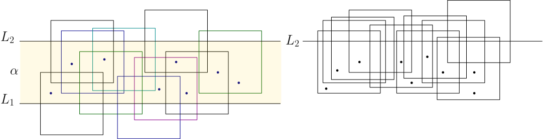
Let and be two sets of points in and be a set of axis-parallel unit squares. We want to approximate the minimum-membership set cover (abbr. MMSC) of using where membership is defined with respect to . First, we divide the plane into horizontal slabs of unit height. Each slab is defined by two horizontal lines and , unit distance apart, where is above . We define an instance for the slab subproblem below. For an illustration, refer to Figure 1.
Definition 3 (Slab instance)
Consider a set of unit squares where each square intersects one of the boundaries of a unit-height horizontal slab . The points of the set to be covered are located within , each point lying inside at least one of the squares in . Let be a set of points with respect to which the membership is to be computed. The instance is called a slab instance.
In section 2.2, we solve the slab instance by decomposing it into two line instances. In the following section, we define and discuss the line instance.
2.1 GMMGSC for the Line Instance
Definition 4 (Line instance)
Consider a set of unit squares where each square intersects a horizontal line . The points of the set to be covered are located only on one side (i.e., above or below) of , each point lying inside at least one of the squares in . Let be a set of points with respect to which the membership is to be computed. The instance is called a line instance.
In the rest of this section, we design an algorithm for the line instance where the points in lie below the defining horizontal line. For the slab, it would be the instance corresponding to the top boundary line of the slab. Refer to Figure 1 for an example. The algorithm for the line instance corresponding to the bottom boundary line is symmetric.
Let us introduce some notation first. For a unit square , denote by and the -coordinate and -coordinate of the bottom-left corner of , respectively. For a horizontal line , denote by the -coordinate of any point on .
We make the following non-degeneracy assumptions. First, no input square has its top boundary coinciding with the slab boundary lines. Second, - and -coordinates of the input squares are distinct. Note that a set of intersecting unit squares also forms a clique in the intersection graph of , and vice versa.
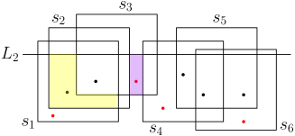
In a set of unit squares , two squares are consecutive (from left to right) if there exists no square such that . If a point is contained in exactly one square in a set cover of a set of points , then is said to be an exclusive point of the square with respect to . For , the region in the plane, denoted by , which is covered exclusively by is called the exclusive region of with respect to a set cover . For , the region in the plane, denoted by , which is contained exclusively in , is called the pairwise exclusive region of and with respect to a set cover . A square in a set cover of a set of points is called redundant if it covers no point of exclusively. Refer to Figure 2 for an illustration of these terms.
A set of unit squares having a common intersection is said to form a geometric clique. A set of unit squares containing a point of in their common intersection region is said to form a discrete clique. The common intersection region of a set of unit squares forming a clique is called the ply region of . The ply region of a clique is always rectangular. For a clique , denote by (resp. ) the -coordinate of the left (resp. right) boundary of the ply region of . Unless specified otherwise, a clique refers to a discrete clique.
2.1.1 Types of legal cliques
First, we classify a clique with respect to a line instance. A set of intersecting squares in a line instance is called a top-anchored clique when the points to be covered lie below the line with respect to which the line instance is defined. A set of intersecting squares in a line instance is called a bottom-anchored clique when the points to be covered lie above the line with respect to which the line instance is defined.
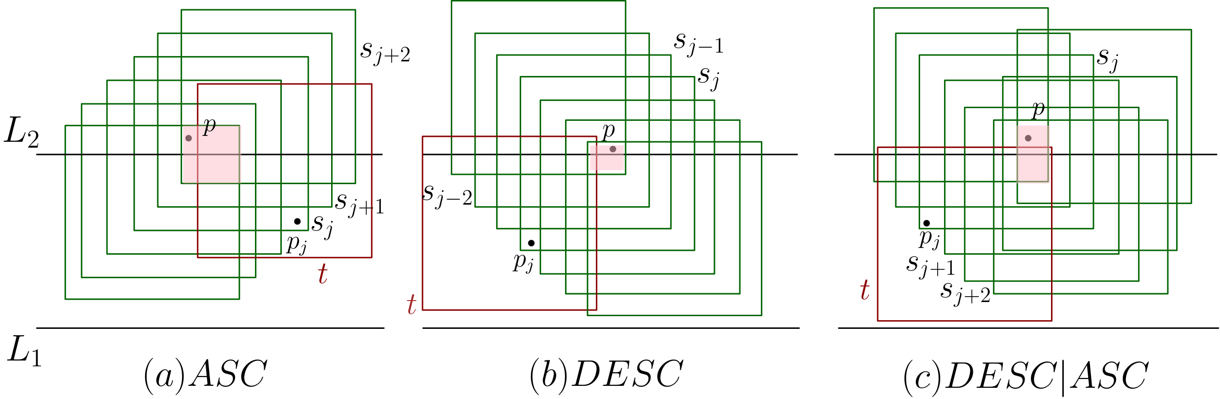
Let a line instance be defined with respect to a horizontal line . Let be a sequence of squares from left to right having a common intersection. This set of squares is called a monotonic ascending clique if implies , for all . We use the abbreviation to denote such a clique. On the other hand, if implies , for all , then this set of squares is called a monotonic descending clique. We use the abbreviation to denote such a clique.
Let a line instance be defined with respect to a horizontal line . Let be a sequence of squares from left to right having a common intersection. This set of squares is called a composite clique if the following holds.
-
•
The sequence of squares forms a monotonic clique.
-
•
Either , or , and
-
•
The sequence of squares forms a monotonic clique.
The square is called the transition square. We use the abbreviation to denote a composite clique where the sequence is descending but the sequence is ascending. For other types of composite cliques, the abbreviation would be self-explanatory.
Claim
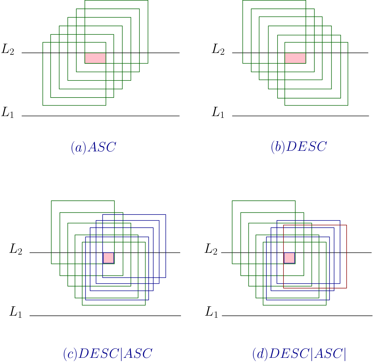
In a set cover for the line instance, where none of the constituent squares are redundant, a top-anchored composite clique must be of type .
Proof
Suppose not. Let be a top-anchored composite clique of type , where the left ascending sequence be the squares from left to right. Then the square would become redundant since the two squares , would cover all the points covered by lying below the defining horizontal line. This contradicts the non-redundancy condition. For an example, refer to Figure (4). Similar arguments apply to rule out the existence of top-anchored composite cliques of type and .
In the rest of the paper, whenever we consider a top-anchored clique in the solution (containing no redundant squares) of a line instance of the GMMGSC problem, we assume that the clique is of one of the following legal types: (i) monotonic , (ii) monotonic , or (iii) composite .
2.1.2 The Algorithm
In this subsection, we describe an algorithm for the line instance that produces a feasible set cover with some desirable structural properties. Multiple maximum cliques may exist in the intersection graph of . We order the maximum cliques of in the increasing order of the values of their ply regions.
Definition 5 (Leftmost maximum clique)
The leftmost maximum clique of a set of unit squares refers to that maximum clique in the intersection graph of for which value of the corresponding ply region is the minimum among all the maximum cliques in .
The procedure consists of the deletion of a set of squares from a set cover and the addition of a square into .
Definition 6 (Profitable swap)
The operation is a profitable swap if is a set of two or more consecutive squares in the leftmost maximum clique , and such that is a feasible set cover for .
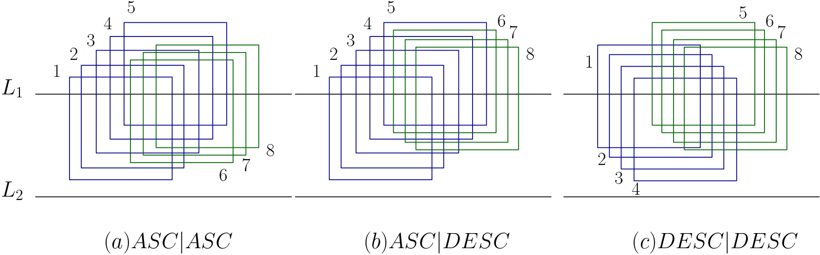
The procedure ensures that each square contains at least one point exclusively. We proved that in a set cover for the line instance, where none of the constituent squares are redundant, any maximum clique can be of only types, as shown in Figure 5.
The algorithm for the line instance is given in Algorithm 1 and has two steps. In the first step, is applied on the set of input squares to obtain a feasible set cover containing no redundant squares. The second step performs a set of profitable swaps on . This step aims to obtain a feasible solution with a maximum clique with some desirable properties. A profitable swap is defined on the leftmost maximum clique of a feasible solution. Refer to Definition 6. We have the following observation about the solution.
{observation}
There exist no profitable swaps on the leftmost maximum clique of returned by Algorithm 1.
Our algorithm implicitly implies the following lemma.
Lemma 1 (Key Lemma)
Let be the leftmost maximum clique in the solution returned by Algorithm 1. Let and be the squares of from left to right. No input square contains , where .
Proof
Fix an index with . Suppose for the sake of contradiction that there exists an input square that covers . Observe that is a profitable swap in , which is a contradiction to Observation 2.1.2.
First, we will show how to implement the algorithm and analyze the running time.
The procedure can be implemented in time.
Proof
Consider an arbitrary ordering of the points in and an arbitrary ordering of the squares in . In time, we construct an matrix where the -th entry is if the -th point is contained in the -th square. Also, construct an array of length . For every point , stores the number of squares in that contain . Initialize each entry of an -length array to . Run a loop that iterates over each square . If does not contain any point with , remove , i.e., set . Set each entry in the -th column of to zero. For each point , decrease by one. At the end of the loop, output the squares with . Naively, the time required to perform all the operations is .
Theorem 2.1
The running time of Algorithm 1 is .
Proof
To compute the leftmost maximum clique in , we obtain the set of squares containing each point of . This takes time.
We need to check if there exists a profitable swap in . There are at most choices for the swapped-in square . While computing , one could also obtain the left-to-right ordering of the squares in . For each candidate swapped-in square , we find a set of consecutive squares that can lead to a profitable swap of by . We can use binary search on the squares of to do this. This requires time. Additionally, we may need to check if the extreme two squares of , say and , can be swapped out safely. This is equivalent to checking if all points in are covered by . Naively, the time required to check this is . Thus, if one exists, we can execute a profitable swap in in time.
We need to remove from those squares in that may have become redundant because of swapping in the square . This can be done by re-invoking on in time (due to Observation 2.1.2). The leftmost maximum clique in can be determined in time.
Every profitable swap decreases the size of the set cover by at least one. Therefore, at most profitable swaps are performed. Thus, there are at most iterations of the while loop. Hence, the total running time of the while loop is .
2.1.3 Structural Properties of the solution
We state two properties about the structure of the solution returned by Algorithm 1. Let be the leftmost maximum clique in the solution returned by Algorithm 1 for the line instance . Let be the squares of from left to right. For , let be the bottom-most exclusive point in .
Lemma 2
Let be an arbitrary point contained in the common intersection region of . For , there exists a set with such that every input square containing also contains , for .
Proof
There are two cases to consider.
-
Case 1:
is a monotonic clique. There are two subcases.
-
•
is a monotonic descending clique. Define the set . By definition , for each . Let be an input square that contains but not . Again, there are two cases.
-
–
lies to the right of , i.e. : Observe that . Since and does not contain , therefore starts before starts, i.e., . Since contains , hence must end below the bottom boundary of and should end to the right of where starts, i.e., and . Combining these with the fact that is a unit square, must cover as shown in Figure 5(b). This is a violation of Lemma 1.
-
–
does not lie to the right of but is above , i.e., but : The square must end after starts, i.e., . Since , the square must end below , i.e., . Since , therefore . So, covers . This is a violation of Lemma 1.
-
–
-
•
is a monotonic ascending clique. Define the set . By definition , for each . Let be an input square that contains but not . By an analogous argument, would be forced to cover either (when lies to the left of as shown in Figure 5(a)) or (when does not lie to the left of but lies above ). This is again a violation of Lemma 1.
-
•
-
Case 2:
is a composite clique (of type ). Let be the index (in the left-to-right ordering) of the bottom-most square in . Define the set . Using the two subcases in the previous case, we can arrive at a violation of Lemma for . Refer to Figure 5(c) for an illustration.
Lemma 3
For , there exists a set with such that no input square can contain for .
Proof
There are two cases to consider.
-
Case 1:
is a monotonic clique. There are two subcases.
-
•
is a monotonic descending clique. Define the set .
-
•
is a monotonic ascending clique. Define the set .
For , assume that contains the bottom-most exclusive points of three consecutive squares of , namely respectively. Then would contain either or . This implies a violation of Lemma 1, as can be seen in Figure 5. Thus, we have a contradiction.
-
•
-
Case 2:
is a composite clique (of type ). Let be the index (in the left-to-right ordering) of the bottom-most square in . We define the set . If , then are in a monotonic descending sequence and the corresponding subcase from Case applies. If , then are in a monotonic ascending sequence and the corresponding subcase from Case applies.
2.2 GMMGSC for the Slab Instance
In this section, we present a constant approximation algorithm for the slab instance. We will use an LP relaxation (adapted from Bandyapadhyay et al. [3]) to partition the slab instance into two line instances.
For each unit square , we create a variable , indicating whether is included in our solution. In addition, create another variable , which indicates the maximum number of times a point in is covered by our solution. Then, we formulate the following linear programming relaxation.
The input set of squares is partitioned naturally into two parts where (resp. ) consists of the input squares intersecting the bottom (resp. top) boundary line (resp. ) of the horizontal slab, say .
We partition the set of points within into and using the LP. Let be an optimal solution of the above linear program computed using a polynomial-time LP solver. For a point and , define as the sum of for all satisfying . Then we assign each point to , where is the index that maximizes .
Now we solve the two line instances , for using Algorithm 1. Finally, we output the union of the solutions of these two line instances. We discard redundant squares from the solution, if any. For , denote by the solution returned by Algorithm 1 for the line instance . We state and prove the following useful lemma.
Lemma 4
For every , , where is the solution returned by Algorithm 1 for the instance and is the minimum membership for the slab instance.
Proof
We consider the case when , i.e., all the squares intersect the top boundary line of the slab . The argument for the case of is identical and is not duplicated. Consider the leftmost maximum clique in the intersection graph of the squares in . Suppose, and the squares in from left to right are .
If , then is satisfied trivially since .
Assume that . Denote by the bottom-most exclusive point of . Let be any point in contained in the ply region of . By Lemma 2, for each , every input square containing also contains . By Lemma 3, no input square contains for . Thus we can write
Since a variable may appear at most twice in the double-sum on the right-hand side, we have multiplied by the factor . The left-hand side of the above inequality is bounded above by the LP optimal . Since every belongs to , we have from the partitioning criteria of into and . From the proofs of Lemma 2 and Lemma 3, we observe that , irrespective of the type of clique . So we can write
By definition, the optimal ply value, , is at least . Therefore, .
Lemma 5
For , let be the solution for the line instance obtained via Algorithm 1. Then is a feasible solution to the slab instance with .
Proof
Since , so is a feasible set cover for the slab instance . Consider an arbitrary point . Using Lemma 4 for , we get that the number of unit squares in containing is at most . Thus, .
2.3 Putting everything together
Theorem 2.2
GMMGSC problem admits an algorithm that runs in time, and computes a set cover whose membership is at most , where denotes the minimum membership.
Proof
We divide the plane into unit-height horizontal slabs. For each non-empty slab , we partition the slab instance into two subproblems, namely the line instances corresponding to the boundary lines of using the LP-relaxation technique described in Section 2.2. We solve each line instance using Algorithm 1. Then we output the union of the solutions thus obtained while discarding redundant squares, if any. Consider any point . Suppose lies within a slab whose boundary lines are and . Since the squares containing must intersect either or , can be contained in squares from at most subproblems. One is a line instance corresponding to where the points lie above . The other is a line instance corresponding to where the points lie below . The other two subproblems correspond to . Thus, due to Lemma 4, the number of squares of our solution containing is at most , where is the optimal membership value for the instance .
References
- [1] Agarwal, P.K., Pan, J.: Near-linear algorithms for geometric hitting sets and set covers. In: Proceedings of the Thirtieth Annual Symposium on Computational Geometry. p. 271–279. SOCG’14, Association for Computing Machinery, New York, NY, USA (2014). https://doi.org/10.1145/2582112.2582152
- [2] Allen-Zhu, Z., Orecchia, L.: Nearly linear-time packing and covering lp solvers. Mathematical Programming 175(1), 307–353 (May 2019). https://doi.org/10.1007/s10107-018-1244-x
- [3] Bandyapadhyay, S., Lochet, W., Saurabh, S., Xue, J.: Minimum-Membership Geometric Set Cover, Revisited. In: 39th International Symposium on Computational Geometry (SoCG 2023). Leibniz International Proceedings in Informatics (LIPIcs), vol. 258, pp. 11:1–11:14 (2023). https://doi.org/10.4230/LIPIcs.SoCG.2023.11
- [4] Biedl, T., Biniaz, A., Lubiw, A.: Minimum ply covering of points with disks and squares. Computational Geometry 94, 101712 (2021). https://doi.org/10.1016/j.comgeo.2020.101712
- [5] Chan, T.M., Grant, E.: Exact algorithms and apx-hardness results for geometric packing and covering problems. Computational Geometry 47(2, Part A), 112–124 (2014). https://doi.org/10.1016/j.comgeo.2012.04.001, special Issue: 23rd Canadian Conference on Computational Geometry (CCCG11)
- [6] Chan, T.M., Hu, N.: Geometric red–blue set cover for unit squares and related problems. Computational Geometry 48(5), 380–385 (2015). https://doi.org/10.1016/j.comgeo.2014.12.005, special Issue on the 25th Canadian Conference on Computational Geometry (CCCG)
- [7] Clarkson, K.L., Varadarajan, K.: Improved approximation algorithms for geometric set cover. Discrete & Computational Geometry 37(1), 43–58 (Jan 2007). https://doi.org/10.1007/s00454-006-1273-8
- [8] Durocher, S., Keil, J.M., Mondal, D.: Minimum ply covering of points with unit squares. In: WALCOM: Algorithms and Computation: 17th International Conference and Workshops, WALCOM 2023, Hsinchu, Taiwan, March 22–24, 2023, Proceedings. p. 23–35. Springer-Verlag, Berlin, Heidelberg (2023). https://doi.org/10.1007/978-3-031-27051-2_3
- [9] Erlebach, T., van Leeuwen, E.J.: Approximating geometric coverage problems. In: Proceedings of the Nineteenth Annual ACM-SIAM Symposium on Discrete Algorithms. p. 1267–1276. SODA ’08, Society for Industrial and Applied Mathematics, USA (2008)
- [10] Feige, U.: A threshold of ln n for approximating set cover. J. ACM 45(4), 634–652 (jul 1998). https://doi.org/10.1145/285055.285059
- [11] Fowler, R.J., Paterson, M.S., Tanimoto, S.L.: Optimal packing and covering in the plane are np-complete. Information Processing Letters 12(3), 133–137 (1981). https://doi.org/10.1016/0020-0190(81)90111-3
- [12] Hochbaum, D.S., Maass, W.: Approximation schemes for covering and packing problems in image processing and vlsi. J. ACM 32(1), 130–136 (jan 1985). https://doi.org/10.1145/2455.214106
- [13] Ito, T., ichi Nakano, S., Okamoto, Y., Otachi, Y., Uehara, R., Uno, T., Uno, Y.: A polynomial-time approximation scheme for the geometric unique coverage problem on unit squares. Computational Geometry 51, 25–39 (2016). https://doi.org/10.1016/j.comgeo.2015.10.004
- [14] Kuhn, F., von Rickenbach, P., Wattenhofer, R., Welzl, E., Zollinger, A.: Interference in cellular networks: The minimum membership set cover problem. In: Wang, L. (ed.) Computing and Combinatorics. pp. 188–198. Springer Berlin Heidelberg, Berlin, Heidelberg (2005)
- [15] Mustafa, N.H., Raman, R., Ray, S.: Settling the apx-hardness status for geometric set cover. In: 55th IEEE Annual Symposium on Foundations of Computer Science, FOCS 2014, Philadelphia, PA, USA, October 18-21, 2014. pp. 541–550. IEEE Computer Society (2014). https://doi.org/10.1109/FOCS.2014.64
- [16] Mustafa, N.H., Ray, S.: Improved results on geometric hitting set problems. Discrete & Computational Geometry 44(4), 883–895 (Dec 2010). https://doi.org/10.1007/s00454-010-9285-9
- [17] Raz, R., Safra, S.: A sub-constant error-probability low-degree test, and a sub-constant error-probability pcp characterization of np. In: Proceedings of the Twenty-Ninth Annual ACM Symposium on Theory of Computing. p. 475–484. STOC ’97, Association for Computing Machinery, New York, NY, USA (1997). https://doi.org/10.1145/258533.258641