Diffusion Noise Feature: Accurate and Fast Generated Image Detection

Abstract

Generative models have reached an advanced stage where they can produce remarkably realistic images. However, this remarkable generative capability also introduces the risk of disseminating false or misleading information. Notably, existing image detectors for generated images encounter challenges such as low accuracy and limited generalization. This paper seeks to address this issue by seeking a representation with strong generalization capabilities to enhance the detection of generated images. Our investigation has revealed that real and generated images display distinct latent Gaussian representations when subjected to an inverse diffusion process within a pre-trained diffusion model. Exploiting this disparity, we can amplify subtle artifacts in generated images. Building upon this insight, we introduce a novel image representation known as Diffusion Noise Feature (DNF). DNF is an ensemble representation that estimates the noise generated during the inverse diffusion process. A simple classifier, e.g., ResNet, trained on DNF achieves high accuracy, robustness, and generalization capabilities for detecting generated images, even from previously unseen classes or models. We conducted experiments using a widely recognized and standard dataset, achieving state-of-the-art effects of Detection.

1 Introduction

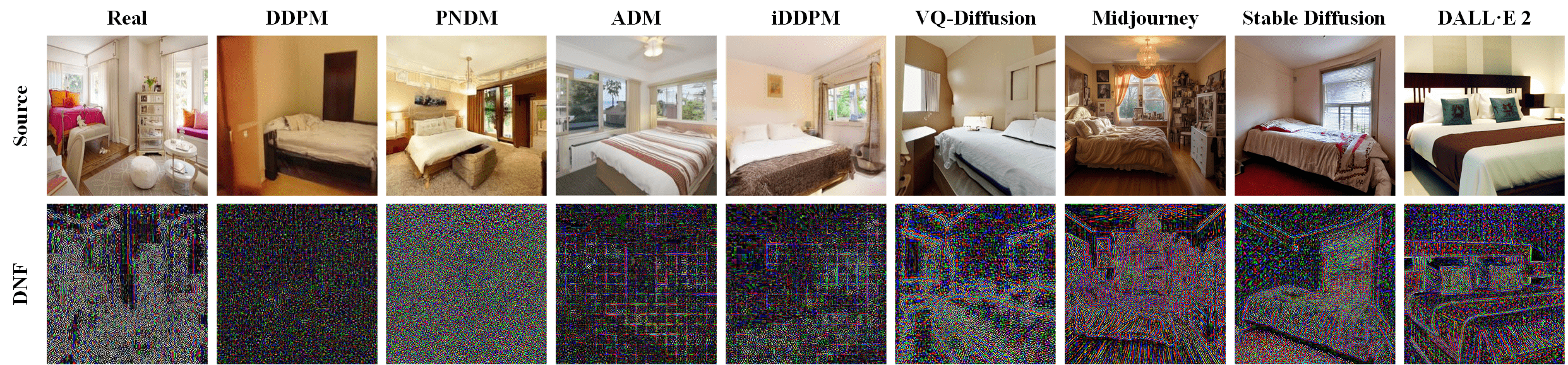
Figure 1: The DNF representation of a real image and eight generated images from different generators. We provide nine pairs of images (Source-DNF) from LSUN-Bedroom [34] and DDPM [14], PNDM [19], ADM [8], iDDPM [23], VQ-Diffusion [13], Midjourney [21], Stable Diffusion [27], DALL·E 2 [26]. The DNF of real images can partially capture the information from the original images but not completely. On the other hand, the DNF of generated images exhibits various types, including pure noise(e.g.,DDPM, PNDM), periodic artifacts(e.g.,ADM, iDDPM), or rich details similar to the original images(e.g.,Midjourney, Stable Diffusion, DALL·E 2), depending on the generative model. By leveraging these features, we can achieve detection of the generated images.

Generative models have achieved remarkable success in recent years, with Denoising Diffusion Probabilistic Models [14] serving as a catalyst for a series of image generation models [8, 30, 27]. These models, owing to their large-scale training datasets and parameters, are capable of generating highly realistic photos. However, the widespread use of these models has also introduced potential risks, including the dissemination of false information [3, 12, 24], the fabrication of evidence [9], privacy breaches [22], and fraudulent activities [31]. For instance, malicious actors can leverage generative models to create convincing fake images for activities such as telecommunications fraud, which can result in immeasurable losses. Consequently, the need to detect whether an image is real or generated has become an urgent and critical problem that requires attention.

At the same time, several detection methods have been developed [32, 6, 25, 2]. While these methods have proven effective in dealing with images synthesized by previous models like GANs, they often struggle to detect images generated by the SOTA generative models, e.g., DALL·E and Stable Diffusion. This is because the realism of the generated results have minimized the distinctions between fake and real images. I.e., the features designed for detection in previous methods are no longer robust enough to differentiate effectively between real and fake images. To address this challenge, two primary approaches should be considered. One approach involves extending the current classifiers for detection. However, even with highly capable models, minor differences between real and fake data can often lead to failures in classification. The alternative approach, which is the central focus of this paper, is to design a novel representation with exceptional generalization capabilities that can significantly improve the detection of generated images.

In this paper, we introduce a novel representation for fake image detection, known as Diffusion Noise Feature (DNF). DNF sets itself apart from previous methods, which manually extract features from real and fake images in spatial or frequency domains. Instead, we leverage the capabilities of contemporary large-scale diffusion models to construct our desired representation. The rationale behind this approach is that these large-scale models are trained to capture the distribution of real images, and they incorporate effective inversion strategies. In other words, we can invert a given image into the latent space of a pre-trained diffusion model. The minor pixel-level differences between real and fake data are magnified during this process, as the artifacts in fake images result in sub-optimal inversions that deviate from those of real data.

To implement this motivation, we take the image to be detected and input it into a pre-trained diffusion model, subsequently conducting an inverse diffusion process. During this process, we collect the estimated noise generated at each step, and then employ an ensemble strategy to integrate these estimated noises into DNF. In Fig. 1, we provide a visualization of DNF. Notably, we observe that real and fake images yield distinct DNF patterns, with fake image DNFs exhibiting various characteristics such as pure noise or periodic artifacts. Leveraging these amplified differences between real and fake images, even a classifier with a simple structure can achieve effective detection, showcasing robust generalization capabilities across diverse data and generative models.

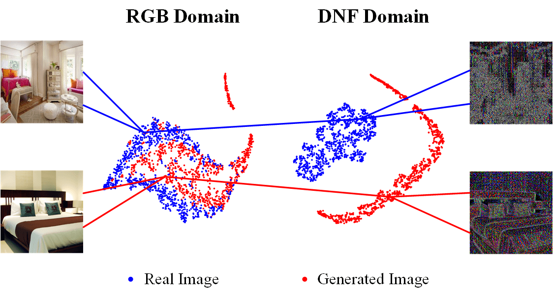
Figure 2: Illustration of the distribution difference between real image and generated image in the image domain and DNF domain. This image demonstrates the helpful role of DNF in classification. By separating the generated image distribution from the real image distribution, a DNF-based classifier can achieve high precision and strong generalization performance in fake detection. Visually, we can see that the two images on the left are difficult to distinguish between real and fake, while the two images on the right show apparent differences. The fake image retains only some of the original image’s information and is occupied with the noise, while the real image exhibits a significant amount of detailed information from the original image.

Extensive experiments and thorough evaluations have been conducted to validate the effectiveness of DNF. Notably, the classifier trained based on DNF consistently achieved remarkable results. (1) The classifier, when trained using DNF, demonstrated 100% accuracy in both validation and testing, which significantly surpassed the average accuracy of 87.4% achieved by the same classifiers trained with other representations. (2) DNF also displayed exceptional robustness. Even when the original image underwent operations such as Gaussian blur and JPEG compression, which can often occur during network transmission, the DNF-based classifier still achieved classification with an accuracy exceeding 99%. (3) DNF owns exceptional generalization performance. For instance, a classifier trained based on LSUN-Bedroom [34] data could outperform similar classifiers when detecting fake images generated by models trained on datasets such as ImageNet [7] and CelebA [20]. (4) DNF demonstrated the capability to detect images generated by unseen models during training. This advantage empowers the classifier to effectively detect generated images when facing entirely new generative models, which is a significant advantage in dynamic and evolving settings.

Our main contributions can be summarized as follows:

• We introduce DNF, a novel and versatile image representation feature derived from the diffusion process, designed for the detection of generated images.

• Extensive experiments are conducted to evaluate DNF in detecting generated images, and the results showcase its state-of-the-art performance.

• We further conduct testing under real-world conditions, placing particular emphasis on evaluating the models’ performance when dealing with images generated by previously unseen models and data categories.

2 Related Work

In this section, we will present the most advanced generative models currently available, along with generative image detection methods.

2.1 Image Generation

The advent of the Diffusion Model has transformed image generation, empowering generators based on diffusion models to create realistic images indistinguishable to the human eye [27, 26]. Additionally, these models demonstrate promise in accommodating multimodal inputs, facilitating content control through straightforward prompts. Zhang et al. [35] enhanced text-to-image generation by refining the network structure of diffusion models for improved content control, while Rombach et al. [27] applied diffusion in the latent image space, embedding conditional controls to achieve high-quality image generation. Notably, the widely acclaimed Stable Diffusion XL [27] and DALL·E series [26] have recently pushed the boundaries of diffusion models, offering unique generation ability.

The capability of these methods to produce high-quality images stems largely from the introduction of DDPM and the adoption of DDIM for expedited inference. The DDPM [14] initially proved adept at generating high-quality images. Subsequently, an increasing number of researchers have dedicated efforts to refining diffusion models, encompassing enhancements to model structures [8, 27] and acceleration of sampling speeds [18, 13]. A notable breakthrough in this domain is credited to Song et al. [14], whose insight into recasting the denoising process in DDPM as a non-Markovian process significantly enhances inference speed. This breakthrough paved the way for the development of Diffusion Models with Invertible Noise [30], facilitating both high-speed and high-quality image generation.

2.2 Generated Image Detection

To address the risks associated with generated images, fake image detection has garnered considerable attention. A notable approach comes from Wang et al. [32], who investigated the commonalities of CNN generators in the frequency domain, leading to the development of the first universal CNN-based image detector through various post-processing methods. Similarly, Wang et al. [33] achieved successful detection of diffusion model-generated images by leveraging differences reconstructed through diffusion models, resulting in high detection accuracy on specific datasets. Moreover, Shi et al. [28] employed a dual-directional reconstruction approach for image detection. In contrast to reconstruction-based methods, Qian et al. [25] focused on analyzing the frequency characteristics of images, extracting necessary information for classification directly from the frequency domain. Frank et al. [10] utilized discrete cosine transform to identify differences in the frequency domain between images from different distributions, enabling the detection of generated images.

However, current detectors fall short of meeting the increasing demand for generalized detection across various distributions. Hence, we are actively pursuing a feature that can be universally applied to detect generated images with diverse content and from different generators.

3 Method

Our method obtains a set of estimated noises by performing an inverse diffusion process on the image to be detected using a pre-trained diffusion model, and converts this set of estimated noises into the Diffusion Noise Feature (DNF) corresponding to this image by a specified ensemble method. In the following sections, we will first introduce the relevant background of the diffusion model (Sec. 3.1), and then give the implementation details of DNF (Sec. 3.2).

3.1 Diffusion Model

Given an initial data distribution $\mathbf{x}_{0}\sim q(\mathbf{x}_{0})$, DDPM [14] uses a manually designed Markov chain to invert the data to a noise distribution according to Eq. 1. Then, a Markov chain trained by a model is used to gradually restore the noise back to the original image according to Eq. 2.

$$q(\mathbf{x}_{t}|\mathbf{x}_{t-1})=\mathcal{N}(\mathbf{x}_{t};\sqrt{1-\beta_{t}}\mathbf{x}_{t-1},\beta_{t}\mathbf{I}),$$ (1)

$$p_{\theta}(\mathbf{x}_{t-1}|\mathbf{x}_{t})=\mathcal{N}(\mathbf{x}_{t-1};\mathbf{\mu}_{\theta}(\mathbf{x}_{t},t),\mathbf{\Sigma}_{\theta}(\mathbf{x}_{t},t)),$$ (2)

where $\beta$ is a hyperparameter that controls the way noise is added in the inverse diffusion process. $\theta$ represents the parameters learned by the model during the training process. Moreover, $\mathbf{\mu}_{\theta}$ and $\mathbf{\Sigma}_{\theta}$ denote the mean and covariance decided by the model during the diffusion process, respectively.

In DDIM [30], this traditional diffusion process is greatly improved, allowing the iterative process to be significantly accelerated without the Markov assumption. DDIM [30] can sample $\mathbf{x}_{t-1}$ from $\mathbf{x}_{t}$ via

$$\begin{split}\mathbf{x}_{t-1}&=\sqrt{\alpha_{t-1}}\left(\frac{\mathbf{x}_{t}-\sqrt{1-\alpha_{t}}\epsilon_{\theta}^{t}(\mathbf{x}_{t})}{\sqrt{\alpha_{t}}}\right)\\ &+\sqrt{1-\alpha_{t-1}-\sigma^{2}_{t}}\cdot\epsilon_{\theta}^{t}(\mathbf{x}_{t})+\sigma_{t}\epsilon_{t},\end{split}$$ (3)

where $\epsilon_{t}\sim\mathcal{N}(0,\mathbf{I})$ is standard Gaussian noise independent of $\mathbf{x}_{t}$, $\epsilon_{\theta}^{t}(\mathbf{x}_{t})$ represents the estimated noise generated by the model at time step $t$ and $\alpha$ is a hyperparameter that controls the diffusion process.

In fact, $\sigma_{t}$ controls the entire diffusion process. For example, when $\sigma_{t}=\sqrt{(1-\alpha_{t-1})/(1-\alpha_{t})}\sqrt{1-\alpha_{t}/\alpha_{t-1}}$, the process in Eq. 3 represents the diffusion process in DDPM [14]. When $\sigma_{t}=0$, the entire forward process is determined by the given $\mathbf{x}_{t}$ and $\mathbf{x}_{0}$.

Let $\sigma_{t}=0$, making it a specified process in DDIM [30]. Assuming $T$ is the total number of steps required in DDPM [14], when $T$ is sufficiently large(e.g., 1000), Eq. 3 can be rewritten for its similarity to Euler integration for solving ODEs.

$$\leavevmode\resizebox{368.57964pt}{}{$\frac{\mathbf{x}_{t-\Delta t}}{\sqrt{\alpha_{t-\Delta t}}}=\frac{\mathbf{x}_{t}}{\sqrt{\alpha_{t}}}+\left(\sqrt{\frac{1-\alpha_{t-\Delta t}}{\alpha_{t-\Delta t}}}-\sqrt{\frac{1-\alpha_{t}}{\alpha_{t}}}\right)\epsilon_{\theta}^{t}(\mathbf{x}_{t})$}.$$ (4)

In this way, the process of inversion can be expressed as

$$\leavevmode\resizebox{368.57964pt}{}{$\frac{\mathbf{x}_{t+1}}{\sqrt{\alpha_{t+1}}}=\frac{\mathbf{x}_{t}}{\sqrt{\alpha_{t}}}+\left(\sqrt{\frac{1-\alpha_{t+1}}{\alpha_{t+1}}}-\sqrt{\frac{1-\alpha_{t}}{\alpha_{t}}}\right)\epsilon_{\theta}^{t}(\mathbf{x}_{t})$}.$$ (5)

In order to achieve the acceleration of Eq. 4 and Eq. 5, we can conduct the sampling of a subsequence $\{\tau_{0},\tau_{1},\ldots,\tau_{S}\}$ from the original sequence $\{0,1,\ldots,T\}$, where $S$ is the total number of steps required in the new process (e.g., 20). The Eq. 5 can be rewrite as

$$\leavevmode\resizebox{368.57964pt}{}{$\frac{\mathbf{x}_{\tau_{t+1}}}{\sqrt{\alpha_{\tau_{t+1}}}}=\frac{\mathbf{x}_{\tau_{t}}}{\sqrt{\alpha_{\tau_{t}}}}+\left(\sqrt{\frac{1-\alpha_{\tau_{t+1}}}{\alpha_{\tau_{t+1}}}}-\sqrt{\frac{1-\alpha_{\tau_{t}}}{\alpha_{\tau_{t}}}}\right)\epsilon_{\theta}^{\tau_{t}}(\mathbf{x}_{\tau_{t}})$}.$$ (6)

In this way, by selecting the subsequence $\{\tau_{i}\}$ appropriately, it is possible to accelerate the entire diffusion process. In our research, this also helps us obtain estimated noise for generating the desired DNF.

3.2 DNF

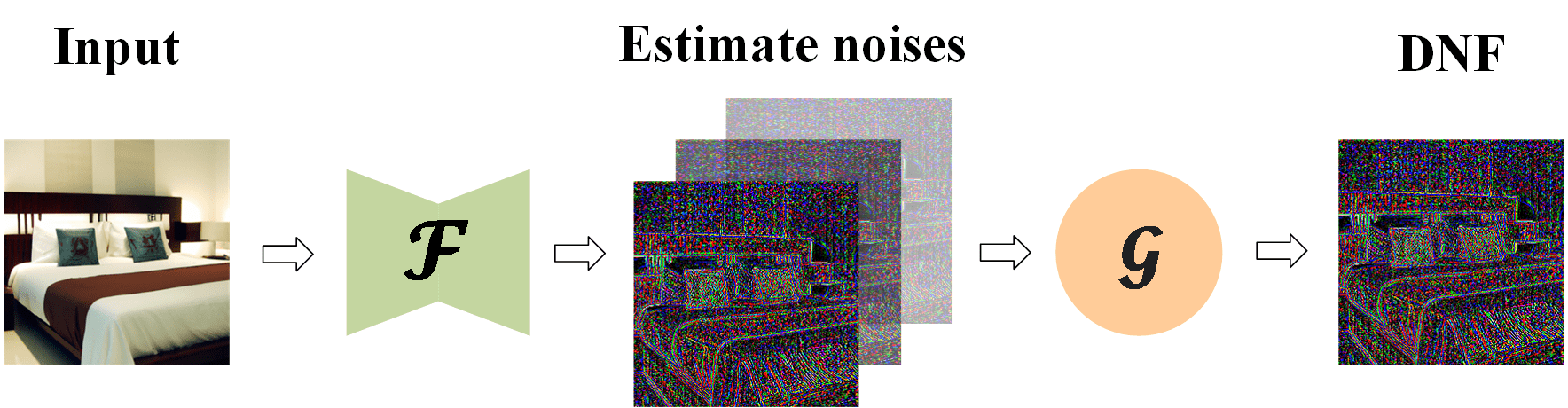
Figure 3: Illustration of computing the DNF representation of inputs. Taking an image as input to a pre-trained diffusion model $\mathcal{F}$ yields a series of estimated noises. These estimated noises are then input into a specified function $\mathcal{G}$ to obtain the corresponding DNF for the input image.

Motivation Given an initial real image distribution $p_{r}(\mathbf{x})$ and a generated image distribution $p_{g}(\mathbf{x})$, the powerful generative capability of existing models allows $p_{g}(\mathbf{x})$ to closely overlap with $p_{r}(\mathbf{x})$, making it challenging for existing discriminators to differentiate samples from these two distributions. Prior approaches have primarily focused on identifying subtle distinctions between $p_{g}(\mathbf{x})$ and $p_{r}(\mathbf{x})$ using methods like frequency domain analysis, which often fail when faced with the realistic images generated by current strong generators (e.g., Stable Diffusion [27]).

Our goal is to devise a novel image representation that characterizes images and transforms the original distributions, $p_{g}(\mathbf{x})$ and $p_{r}(\mathbf{x})$, into new distributions, $p^{\prime}_{g}(\mathbf{x})$ and $p^{\prime}_{r}(\mathbf{x})$, through the use of this representation. These transformed distributions should exhibit sufficient separability, enabling various classifiers to distinguish between real and fake images effectively. In essence, this novel image representation serves to amplify the subtle differences between real and generated images, thereby facilitating the creation of a more precise and broadly applicable generator detector.

In our research, we have observed that as different images undergo the inverse diffusion process in Eq. 6, they produce various types of $\epsilon_{\theta}$. Some $\epsilon_{\theta}$ exhibit periodic pseudo-artifacts, while others display purely noisy characteristics. Subsequent experiments have affirmed that this phenomenon is not substantially influenced by factors such as image content, resolution, or sampling time steps. Instead, it exhibits a strong correlation with the specific generative model used for generating the images. Therefore, we can capitalize on this phenomenon to develop a novel representation.

Implementation We now present the implementation details for computing the DNF for a given image.

Suppose we have an image $\mathbf{x}_{0}$ that needs to be detected and a pre-trained diffusion model $\mathcal{F}$ with parameter _θ. For $\mathcal{F}$, we can obtain an estimated noise for $\mathbf{x}$ at a given time step $t$ via Eq. 7.

$$\epsilon_{\theta}^{t}(\mathbf{x})=\mathcal{F}_{\theta}(\mathbf{x},t).$$ (7)

To compute DNF, we first sample a subsequence $\{\tau_{0},\tau_{1},\ldots,\tau_{S}\}$ from $\{0,1,\ldots,T\}$ (usually using uniform sampling) and set them as time steps in the inverse diffusion process. Following the approach in DDIM, we feed $\mathbf{x}_{0}$ into our prepared model $\mathcal{F}_{\theta}$ and then perform the inverse diffusion process based on Eq. 6. At each step, we obtain an estimated noise $\epsilon_{\theta}^{\tau_{i}}(\mathbf{x}_{\tau_{i}})$ in Eq. 7 corresponding to the time step. We define a set $E$ that contains all these estimated noises.

After completing the entire inverse diffusion process, we use this set of estimated noise $E$ as input to an ensemble functions $\mathcal{G}$. The ensemble function $\mathcal{G}$ is required to facilitate the processing of the estimated noise sets into a unified representation. By computing through $\mathcal{G}$, we finally obtain the DNF corresponding to the input image $\mathbf{x}_{0}$.

The Algorithm 1 presents all these processes. Sample represents a function that samples a subsequence from a given sequence. Typically, we can use equidistant uniform sampling or logarithmic sampling to obtain a subsequence that starts sparse and becomes compact later. append denotes the operation of adding an element to a sequence. Based on Algorithm 1, we can summarize the DNF computation method as Eq. 8. At the same time, we also show this pipeline graphically in Fig. 3.

Input: Input Image $\mathbf{x}_{0}$, Diffusion Model $\mathcal{F}$, Model Parameters $\theta$, Ensemble Function $\mathcal{G}$

Output: $\mathbf{DNF}(\mathbf{x}_{0})$

1 $\{\tau_{0},\tau_{1},\ldots,\tau_{S}\}=\textbf{Sample}(\{0,1,\ldots,T\},S)$

2for $\tau_{i}$ in $\{\tau_{0},\tau_{1},\ldots,\tau_{S}\}$ do

3      

4      $\eta_{i}=\sqrt{\left(1-\alpha_{\tau_{i+1}}\right)/\alpha_{\tau_{i+1}}}+\sqrt{\left(1-\alpha_{\tau_{i}}\right)/\alpha_{\tau_{i}}}$

5      $\mathbf{x}_{\tau_{i+1}}=\sqrt{\alpha_{\tau_{i+1}}/\alpha_{\tau_{i}}}\mathbf{x}_{\tau_{i}}+\eta_{i}\mathcal{F}_{\theta}(\mathbf{x}_{\tau_{i}},\tau_{i})$

6      $E.\textbf{append}\left(\mathcal{F}_{\theta}(\mathbf{x}_{\tau_{i}},\tau_{i})\right)$

7 end for

8

$\mathbf{DNF}(\mathbf{x}_{0})=\mathcal{G}(E)$

Algorithm 1 The algorithm of computing DNF for a given image $x_{0}$.

$$\mathbf{DNF}(\mathbf{x}_{0})=\mathcal{G}(\{\mathcal{F}(\mathbf{x}_{i}),t_{i}\}),\ i\in\{0,1,\ldots,S\}$$ (8)

Implementation of Ensemble Function The specific implementation and evaluation of ensemble function $\mathcal{G}$ will be explained in detail in Sec. 4.5, where we will assess the impact of various ensemble functions on the final results. Here, we define an ensemble function $\mathcal{G}_{i}$ as a function that takes a sequence of inputs and outputs a specified feature. In the subsequent experimental experiments, we will use a function that outputs the first element of a sequence as the ensemble function.

4 Experiments

4.1 Experimental Settings

Dataset. To ensure a fair comparison with existing state-of-the-art methods, we have chosen DiffusionForensics [33] as the dataset for our experiments. DIRE [33] and other state-of-the-art methods are evaluated on this dataset, making it a highly representative benchmark for image generation detection. DiffusionForensics [33] comprises images generated by various models, including ADM [8], DDPM [14], iDDPM [23], LDM [27], PNDM [19], Stable Diffusion-v1 [27], Stable Diffusion-v2 [27], VQ-Diffusion [13], DALL-E 2 [26], IF, and Midjourney [21]. These images encompass categories from LSUN-Bedroom [34], ImageNet [7], and CelebA [20]. By using DiffusionForensics [33], we can thoroughly evaluate the performance of different methods in detecting generated images and ensure the credibility of our experiments.

Data pre-processing and augmentation. Our image processing consists of two parts: preprocessing before computing DNF and preprocessing before training the classifier. Before calculating DNF, we scale all the images from the dataset to a uniform size of 256$\times$256 to ensure that our pre-trained diffusion model on LSUN-Bedroom [34] can accurately calculate the corresponding DNF for each image. Before training or testing the classifier, we resize all the training data to 224$\times$224. Additionally, during the training process, each image undergoes independent horizontal and vertical flips with a probability of 0.5.

Evaluation metrics. In our experiments, we primarily evaluate our model using two metrics: Accuracy (Acc) and Average Precision (AP). The threshold for computing accuracy is set to 0.5.

Baselines. 1) CNNDetection [32] has introduced a detection model trained to distinguish images synthesized from a specific type of CNN model. However, this model exhibits strong generalization ability, meaning it can effectively detect images generated by various CNN models, not just the one it was trained on. 2) SBI [29] is a method applied for DeepFake detection. It trains a universal synthetic image detector by blending fake source images with target images derived from a single original image. This approach enables the detector to learn and recognize synthetic images, regardless of the specific source or target images used in the blending process. 3) Patchforensics [4] utilizes a patch-wise classifier, which has been reported to outperform simple classifiers in detecting fake images. Instead of analyzing entire images, Patchforensics focuses on examining smaller patches within an image to identify inconsistencies or anomalies that indicate image manipulation or forgery. 4) F3Net [25] emphasizes the significance of frequency information in detecting fake images. By analyzing the frequency components of an image, F3Net can identify discrepancies or irregularities that are indicative of image tampering or generation. 5) DIRE [33] conducts detection by leveraging the differences between real images and generated images after utilizing a diffusion model for reconstruction. By comparing the characteristics of reconstructed images with those of genuine images, DIRE aims to identify the presence of artificial manipulation or generation.

Method

Training Dataset

Generation Model

Testing Generators

Total Avg.

ADM

DDPM

iDDPM

LDM

PNDM

SD-v1

SD-v2

VQ-Diffusion

DALL-E 2

IF

Midjourney

CNNDet [32]

LSUN

-

50.1/64.1

56.8/77.4

50.2/78.1

50.1/61.4

50.1/83.4

50.5/81.1

51.9/83.9

50.1/71.5

53.8/82.8

51.1/80.6

51.8/75.8

51.5/76.3

SBI [29]

FF++

-

53.4/60.8

56.9/50.8

58.4/56.2

83.4/90.2

73.1/95.6

54.6/63.3

59.2/70.9

56.2/74.2

51.2/56.4

61.3/72.3

52.3/87.9

52.1/70.7

Patchfor [4]

FF++

-

50.2/67.4

53.2/74.2

51.2/63.4

56.7/89.1

56.5/72.4

42.9/90.2

54.2/72.7

87.2/95.4

50.1/68.9

50.0/56.3

56.1/57.2

55.3/73.3

DIRE [33]

LSUN-B.

ADM

97.9/99.8

96.5/99.8

98.9/99.8

99.8/99.7

99.6/99.4

89.9/99.8

89.9/99.8

89.9/99.8

86.5/99.7

89.9/99.8

81.6/99.0

92.7/99.6

F3Net* [25]

LSUN-B.

-

91.2/97.8

90.7/98.5

89.9/99.2

98.1/100

92.3/97.2

82.7/92.6

81.1/90.4

92.4/97.3

78.1/86.2

73.6/82.2

75.9/81.1

85.9/92.9

CNNDet* [32]

LSUN-B.

-

99.4/99.9

98.9/99.9

99.7/100

97.7/99.6

99.6/100

77.6/95.2

67.7/99.6

88.8/99.5

95.8/99.5

95.2/99.9

65.3/95.8

89.6/98.9

Patchfor* [4]

LSUN-B.

-

94.1/99.8

72.9/98.2

95.2/99.4

97.2/100

94.2/100

72.1/87.6

74.5/90.2

95.4/100

85.2/98.2

65.4/82.3

53.2/88.6

81.7/94.9

DNF(ours)

LSUN-B.

DDIM

100/100

100/100

100/100

100/100

100/100

100/100

100/100

100/100

100/100

100/100

100/100

100/100

LSUN-B.

ADM

100/100

100/100

100/100

100/100

100/100

100/100

100/100

100/100

100/100

100/100

100/100

100/100

ImageNet

DDIM

100/100

100/100

100/100

100/100

100/100

100/100

99.9/100

100/100

100/100

100/100

100/100

99.9/100

ImageNet

ADM

100/100

100/100

100/100

100/100

100/100

100/100

99.7/100

100/100

100/100

100/100

100/100

99.9/100

Table 1: Comparison on the DiffusionForensics. We tested the detection performance of CNNDetection [32], Patchforensics [4], SBI [29], F3Net [25], DIRE [33] and our proposed DNF methods on the test set of the DiffusionForensics [33]. The main evaluation metrics are accuracy(ACC) and average precision(AP). “Training Dataset” represents the dataset on which the model is trained (LSUN-B [34] training set includes ADM [8], DDPM [14], iDDPM [23], LDM [27], PNDM [19], and ImageNet [7] training set includes ADM [8]). “Generation Model” represents the model used to generate input features (if necessary). In our experiments, we made efforts to use the official pre-trained models provided by the corresponding methods. Otherwise, we trained models on DiffusionForensics for evaluation purposes (indicated by * after the method name). Analyzing the experimental results reveals that the DNF method demonstrates a remarkably strong detection capability (achieving 100% accuracy and average precision), while other methods suffer from issues such as insufficient accuracy and data dependency.

4.2 Comparison to Existing Detectors

We compared the performance of our DNF-based classifier with the chosen baselines on DiffusionForensics [33]. When evaluating the baselines, we made an effort to utilize officially released pre-trained parameters for both the feature extractor and the classifier. Additionally, we retrained the trainable components of some baselines on DiffusionForensics to assess their performance more accurately. All the evaluation results are presented in Tab. 1.

From the results, it can be observed that the previously published methods using their pre-trained models cannot effectively detect new types of generated images. Methods represented by CNNDetection [32], SBI [29], and Patchforensics [4] achieved only an average accuracy of 52.3% and an average precision of 73.4%. After retraining CNNDetection [32], F3Net [25], and Patchforensics [4] on DiffusionForensics, they achieved an average accuracy of 94.1% and an average precision of 93.3% on the generator categories encountered during training. However, when encountering unseen generator models, their performance dropped to an average accuracy of 83.4% and an average precision of 92.5%. The best-performing method among the chosen baseline is DIRE [33], which achieved an average accuracy of 92.7% and an average precision of 99.6%. At the same time, our DNF-based method outperforms all others on DiffusionForensics [33], achieving a perfect average accuracy and average precision of 100% in both generator categories and dataset categories. This demonstrates a significant improvement compared to the Baseline.

4.3 Generalization Capability Evaluation

In this section, we will evaluate the generalization capabilities exhibited by different methods in detecting various generators and datasets. From this perspective, we will demonstrate the superiority of DNF in terms of the generalization ability.

Generalization on generator categories. From Sec. 4.2, we can observe that previous methods still achieve high accuracy in detecting generator categories encountered during training. However, when they encounter generator categories that have not been seen before, the accuracy of these detection methods significantly declines. On the other hand, the DNF method still maintains a relatively high accuracy and precision. Most of the generators in Tab. 1 are trained based on diffusion models. To evaluate the generalization performance on different types of generators, we selected five different GANs, BigGAN [1], CycleGAN [36], ProGAN [15], StarGAN [5], StyleGAN [16], for further generalization evaluation. We used test data provided by the official CNNDetection dataset [32], and the results are presented in Tab. 2.

We can conclude that DNF outperforms DIRE in terms of generalization performance when facing generators that were not seen during training and have fundamentally different principles. DNF achieves an accuracy advantage of over 9.2% compared to DIRE. Furthermore, DNF also achieves higher detection accuracy compared to CNNDetection trained on this dataset, which demonstrates the performance of DNF in detecting generators such as GANs. To evaluate DNF’s performance on potential future generators, we assessed its performance on generators likeDALL-E 2 [26], IF, Midjourney [21] and Stable Diffusion XL(SD-XL) [27], as shown in Tab. 1 and Tab. 2. We can confidently conclude that DNF demonstrates stronger cross-model generalization capabilities..

Method	Testing Generators						Total Avg.
	BigGAN	CycleGAN	ProGAN	StarGAN	StyleGAN	SD-XL
CNNDet	70.2/84.5	85.2/93.5	100/100	91.7/98.2	87.1/99.6	49.9/62.3	80.6/90.4
DIRE	89.7/99.5	90.4/99.9	90.1/100	92.8/99.5	90.1/99.8	89.9/99.7	90.6/99.7
DNF(ours)	100/100	100/100	99.9/100	100/100	99.3/100	100/100	99.8/100

Table 2: Cross-generator Evaluation. We used the officially released CNNDetection [32] and DIRE [33] pre-trained models as baselines to investigate the detection capabilities of DNF compared to these two methods on five different GANs: BigGAN [1], CycleGAN [36], ProGAN [15], StarGAN [5], StyleGAN [16]. In addition, we also tested the detection capabilities of these three methods on the emerging generative model SD-XL [27].

Method	T.D.	LSUN-B.		ImageNet		CelabA			Total Avg.
		ADM	SD-v1	ADM	SD-v1	LDM	PNDM	SD-v2
CNNDet	L.B.	99.4/100	77.6/95.2	73.4/86.2	51.8/84.1	54.8/64.2	93.6/99.2	82.9/94.3	64.3/89.0
	I.N.	67.1/59.9	65.6/40.9	80.5/96.1	51.9/72.2	96.0/99.6	87.0/95.3	90.9/97.1	77.0/80.1
	C.A.	51.4/62.9	55.4/76.8	69.2/77.8	33.5/61.0	99.9/100	99.7/100	79.9/94.8	69.8/81.9
DIRE	L.B.	97.9/99.8	89.9/99.8	58.6/68.9	57.3/66.2	64.2/99.7	64.1/98.1	64.2/99.6	70.8/90.3
	I.N.	70.5/97.9	70.5/98.7	99.8/99.9	98.6/99.9	51.4/95.4	50.0/81.0	51.5/96.7	70.3/95.6
	C.A.	65.5/78.7	72.0/90.3	61.4/69.3	58.2/66.2	57.1/68.2	88.2/94.1	94.9/98.9	71.0/80.8
DNF	L.B.	100/100	100/100	99.4/100	99.4/100	100/100	100/100	99.8/100	99.9/100
	I.N.	100/100	100/100	100/100	98.9/100	100/100	100/100	99.9/100	99.8/100
	C.A.	57.9/54.2	56.6/53.5	72.0/64.5	81.1/78.5	100/100	100/100	100/100	81.0/78.6

Table 3: Cross-dataset Evaluation. We trained CNNDetection [32], DIRE [33], and DNF using three different datasets (T.D. represents the training dataset): LSUN-B (L.B.) [34], ImageNet (I.N.) [7], and CelebA (C.A.) [20], to evaluate their cross-dataset generalization performance. The generated images for LSUN-B and ImageNet were obtained from a subset of DiffusionForensics [33], while the generated images for CelebA were produced by models trained on CelebA using LDM [27] and PNDM [19]. Analyzing the data, we found that DNF exhibits the least significant decrease in accuracy when facing cross-dataset detection compared to CNNDetection and DIRE, demonstrating its excellent cross-dataset and cross-category generalization capabilities.

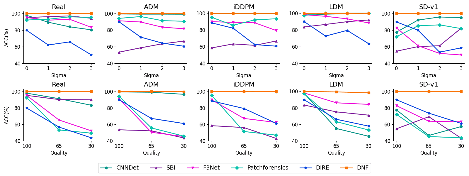
Figure 4: Robustness to Unseen Perturbations. We created a test set by applying specified parameters of Gaussian blur and JPEG compression to the original images. We evaluated the model’s robustness to unseen perturbations by measuring its performance on this fully trained model on the test set. Analyzing the data, we observed that existing forensic methods suffer from accuracy degradation or improvement as the perturbations are introduced, especially in the case of JPEG compression, which leads to severe misclassification of real samples. In contrast, DNF exhibits excellent robustness, with its performance showing minimal fluctuations as the perturbations increase, ensuring an overall accuracy of over 99%.

Generalization on cross-datasets. In Tab. 1, we evaluated the performance of various methods on the LSUN-Bedroom subset of DiffusionForensics [33]. Here, we aim to investigate whether a model trained on one dataset can transfer its detection performance to another unseen dataset. To accomplish this, we designed a cross-datasets generalization evaluation experiment to assess the generalization performance of a model on three datasets: LSUN-Bedroom [34], ImageNet [7], and CelebA [20]. The test results are presented in Tab. 3.

Tab. 3 shows a decline in detection performance for all methods when faced with the task of detecting generated images with anomalies. This phenomenon is more evident in CNNDetection and DIRE, where the overall accuracy can decrease by up to 66.4%. This may be because both methods, CNNDetection and DIRE, have strong data dependencies in their training processes. CNNDetection focuses on learning image features specific to the designated categories in the dataset. For example, features learned in the “bedroom” category may not be applicable to “cat” images. On the other hand, DIRE is influenced by the dataset used to train the diffusion model for reconstruction. For instance, a diffusion model trained on ImageNet may not effectively reconstruct images from the LSUN-B dataset, resulting in a decrease in detection accuracy. However, the DNF method exhibits excellent generalization performance, showing superior performance in cross-dataset detection with models trained on LSUN-B and ImageNet. The only drawback is that models trained on CelebA lack generalization performance in detecting other datasets. This may be due to the dataset primarily focusing on human faces, causing the models to learn more facial-related details and overlook artifacts generated by the models, thus rendering the learned features less applicable to categories such as bedroom, cat, airplane, etc.

4.4 Robustness to Unseen Perturbations

During the process of network transmission, images may undergo certain perturbations (e.g., Gaussian blur [11], JPEG compression [17]), which can disrupt the information contained in the images and consequently hinder the correct detection of whether an image is generated. Therefore, we designed a perturbation robustness experiment to investigate whether various methods can maintain high-performance detection when faced with these blurred or compressed images after training. In this experiment, we set the Gaussian blur $\sigma\in\{0,1,2,3\}$ and JPEG compression $\textit{quality}\in\{100,65,30\}$. We tested the detection performance of the Baseline and DNF methods against these unseen perturbations, and the results are presented in the form of line graphs in Fig. 4.

From Fig. 4, we find that most of the previous methods experience a decrease in accuracy when faced with perturbations. However, there are still some methods (e.g., CNNDetection, SBI, Patchforensics) that show an increase in detection accuracy when presented with images affected by Gaussian blur. This may be because the details in generated images are relatively more susceptible to distortion compared to real images, and these methods prioritize the detection of such details. As a result, they can achieve higher detection accuracy by focusing on these specific aspects. Overall, perturbations have a significant impact on these methods. Meanwhile, the DNF method maintains a detection accuracy of over 99% in the presence of perturbations. It can be said that DNF demonstrates sufficient robustness when facing these two types of perturbations.

4.5 Ablation Analysis on DNF

This section will investigate the impact of selecting different components in DNF computation on detection accuracy, including two aspects: the choice of the pre-trained model $\mathcal{F}$ and the choice of the integration function $\mathcal{G}$.

Effect of choice of inverse diffusion process models. In the process of computing DNF, it is inevitable to use a pre-trained diffusion model $\mathcal{F}$ to perform the inverse diffusion process. In the previous experimental data we provided, we used a model pre-trained on LSUN-Bedroom with DDIM to execute the inverse diffusion process. Considering that different diffusion models may use different methods to control the generation of $\epsilon^{t}_{\theta}$, we also set up a control group using ADM [8] as $\mathcal{F}$. The guide mechanism inside ADM may lead to the generation of $\epsilon^{t}_{\theta}$ being influenced by other factors. The experimental results are presented in Tab. 1. We found that there was no significant difference in detection performance when we switched to a different model for executing the inverse diffusion process. By observing the DNF generated by ADM, we found that although the DNF for images generated by the same generator differs from that generated by DDIM, there is still a significant difference between the DNF of real images and generated images, which is sufficient to help the classifier perform the detection task. In general, the DNF-base method is applicable to the majority of diffusion models currently available.

Method	Testing Generators					Total Avg.
	ADM	iDDPM	LDM	StyleGAN	SD-v1
$\mathcal{G}_{first}$	100/100	100/100	100/100	99.3/100	100/100	99.8/100
$\mathcal{G}_{avg}$	98.2/99.9	99.1/100	97.5/100	98.2/99.9	98.2/100	98.2/99.9
$\mathcal{G}_{last}$	100/100	100/100	100/100	96.2/99.4	93.1/98.8	97.8/99.6

Table 4: Effect of different calculation of DNF. In this test, we tried different DNF calculation methods, and the results show that the First method can give the highest detection performance.

Effect of different calculation of DNF. In our previous experiments, we uniformly used the mentioned $\mathcal{G}_{first}$ as our designated ensemble function. However, there are multiple methods to process an image sequence and obtain an output feature. To explore the impact of different ensemble function choices on the final DNF output and classification accuracy, we designed three different $\mathcal{G}$ functions ($\mathcal{G}_{first}$, $\mathcal{G}_{avg}$, $\mathcal{G}_{last}$). They respectively represent taking the first element of a sequence, taking the average of all elements in a sequence, and taking the last element of a sequence. Their expressions can be referred to in Eq. 9,

$$\small\mathcal{G}_{last}(X)=x_{N},\,\mathcal{G}_{first}(X)=x_{0},\,\mathcal{G}_{avg}(X)=\frac{\sum_{i=0}^{N}x_{i}}{N+1},$$ (9)

where $X=\{x_{0},x_{1},\ldots,x_{N}\}$. We compared the effects of different DNF computation methods on classification accuracy, and the specific results are presented in Tab. 4. We observed that $\mathcal{G}_{first}$ yielded the highest classification accuracy, while $\mathcal{G}_{last}$ corresponded to lower classification accuracy. After visualizing a series of noise sequences $E$ for a set of images, we found that the $\epsilon^{t}_{\theta}$ of an image is generated based on the image $\mathbf{x}_{t}$ itself. This results in the loss of some fine-grained details in the latter part of the sequence $\epsilon^{t}_{\theta}$, as the input image $\mathbf{x}_{t}$ has already been corrupted by noise, thereby containing more information about the noise injection process. This may explain the lower classification accuracy associated with $\mathcal{G}_{last}$. Additionally, using $\mathcal{G}_{first}$ has another important advantage, which is the ability to perform only one step of the inverse diffusion process, significantly reducing the inference time required for DNF computation.

5 Conclusion

In this paper, we introduce a novel image representation feature called DNF and apply it to the task of detecting generated images. We provide extensive experimental evidence to demonstrate that DNF features, when combined with a simple classifier framework, can achieve high accuracy, strong robustness, and generalization performance in detecting generated images. We also explore the impact of different computation methods on DNF outputs and classification accuracy, providing further insights into the underlying mechanisms of DNF.

While our method has demonstrated excellence on public evaluation datasets, such as DiffusionForensics, the continuous development of increasingly effective generators, such as the unreleased DALL-E 3, presents new challenges. Looking ahead, we plan to broaden our detection evaluation scope to encompass a wider array of generators. This involves creating an expansive benchmark to comprehensively assess the performance of various fake image detection frameworks. Moreover, we are committed to ongoing research and development to tailor detection frameworks specifically for DNF, aiming for even better performance in identifying generated images.

We believe that our work can lay a crucial foundation for the field of generated image detection, inspiring researchers to pursue further advancements in this domain.

Supplementary Material

6 Analysis of Noise Sequences

In the main paper, we mentioned that different time steps in the inverse diffusion process generate distinct noise. As the input image gradually approaches pure noise, the corresponding estimated noise $\epsilon$ also varies. We visualize the real image (Fig. 5), ADM-generated image (Fig. 6), and Stable-Diffusion-v2-generated image (Fig. 7) in the inverse diffusion process of DDIM to observe the generated noise.

By observing these noise sequences, we find that the initial generated noise shows the most distinct differences. As time progresses, these noises gradually converge into a grid-like pattern. This is because the model gradually aligns images from different distributions to a unified noise distribution in the inverse diffusion process. Therefore, these noises tend to exhibit the same pattern in the later stages of the inverse diffusion process.

As mentioned in Sec. 4.5 of the main paper, different ensemble functions result in different classification accuracies, with $\mathcal{G}_{first}$ showing the best performance. This conclusion can also be derived from the visualization of the estimated noise sequences, where the difference in $\epsilon_{0}$ is most pronounced. Hence, we choose $\mathcal{G}_{first}$ as our default ensemble function to achieve the optimal classification performance.

7 Analysis of DNF in Frequency Domain

We would like to further analyze why the classifier can successfully detect generated images with the help of DNF. Our initial hypothesis was that DNF, as a new image representation, can amplify the differences between real and generated images in the spatial domain. In this section, we try to verify whether such differences also exist in the frequency domain. To validate this hypothesis, we sampled 1K images from each generator category and performed the Fourier Transform for their DNFs to obtain the corresponding frequency domain distributions. We then calculated the average frequency domain features for each generator category. These features are visualized in Fig. 8.

By analyzing the frequency domain features of the DNF for different generators, we found that the DNF of real images exhibits a smoother frequency domain distribution, while the DNF of generated images often shows periodic patterns. Compared to directly analyzing the frequency domain of the images with RGB values, the frequency domain information of DNF reveals more differences between real and generated images. This confirms our hypothesis and demonstrates that DNF amplifies the differences between real and generated images in varying domains.

8 More Visualization about DNF

We visualize some DNF features of images synthesized from DDPM (Fig. 10), PNDM (Fig. 11), ADM (Fig. 12), LDM (Fig. 13), iDDPM (Fig. 14), VQ-Diffusion (Fig. 15), Stable Diffusion v1 (Fig. 16), Stable Diffusion v2 (Fig. 17), Stable Diffusion XL (Fig. 18), Midjourney (Fig. 19), and DALL-E 2 (Fig. 20). These visualizations include the source images, DNF obtained via DDIM, and DNF derived via ADM.

Analyzing these DNF features, in $\textbf{DNF}_{\textbf{DDIM}}$, the DNF of real images shows rough partial features of the original image, while the DNF of generated images shows pure noise (Fig. 10, Fig. 11), grid-like patterns (Fig. 12, Fig. 14) or a lot of source image features (Fig. 13, Fig. 15, Fig. 16, Fig. 17, Fig. 18, Fig. 20). In $\textbf{DNF}_{\textbf{ADM}}$, the DNF of real images shows a combination of grid-like stripes and original image features. In contrast, the DNF of generated images mostly shows pure noise (Fig. 10, Fig. 11, Fig. 12, Fig. 14, Fig. 16, Fig. 17, Fig. 18), a combination of pure noise and a few original image features (Fig. 15, Fig. 20) or a few show blocky noise composed of original image features (Fig. 13). The difference between $\textbf{DNF}_{\textbf{DDIM}}$ and $\textbf{DNF}_{\textbf{ADM}}$ is determined by the diffusion model that performs the inverse diffusion process. Such differences do not affect the detection of generated images because real images tend to have different distributions from generated images, and will always produce different types of DNFs.

Figure 5: Analysis of Noise Sequences for the Real image.

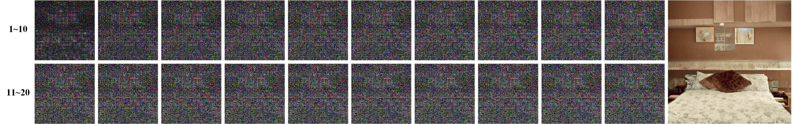
Figure 6: Analysis of Noise Sequences for the ADM [8]-generated image.

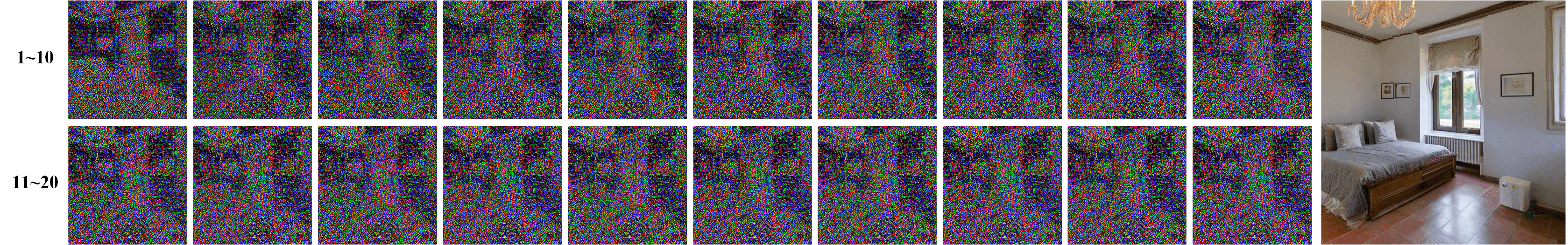
Figure 7: Analysis of Noise Sequences for the SDv2 [27]-generated image.

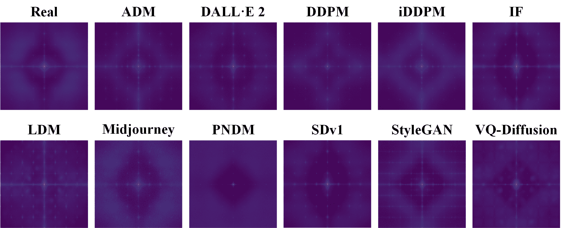
Figure 8: Analysis of DNF in the frequency domain.

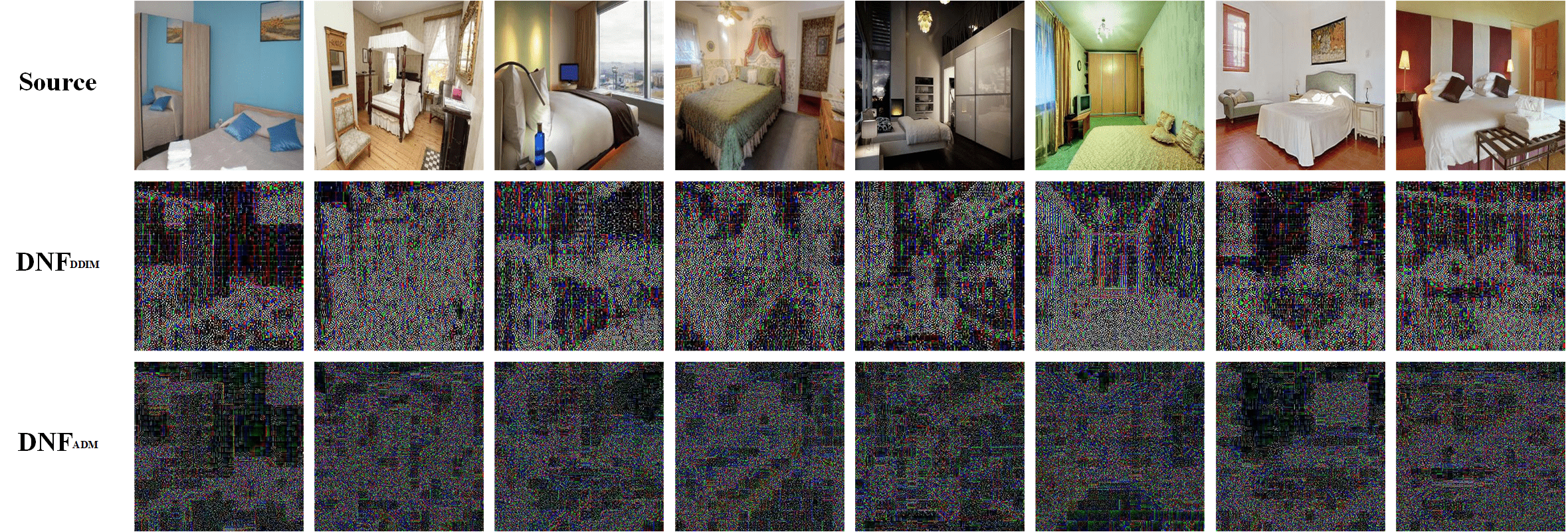
Figure 9: Visualization of DNF for Real images.

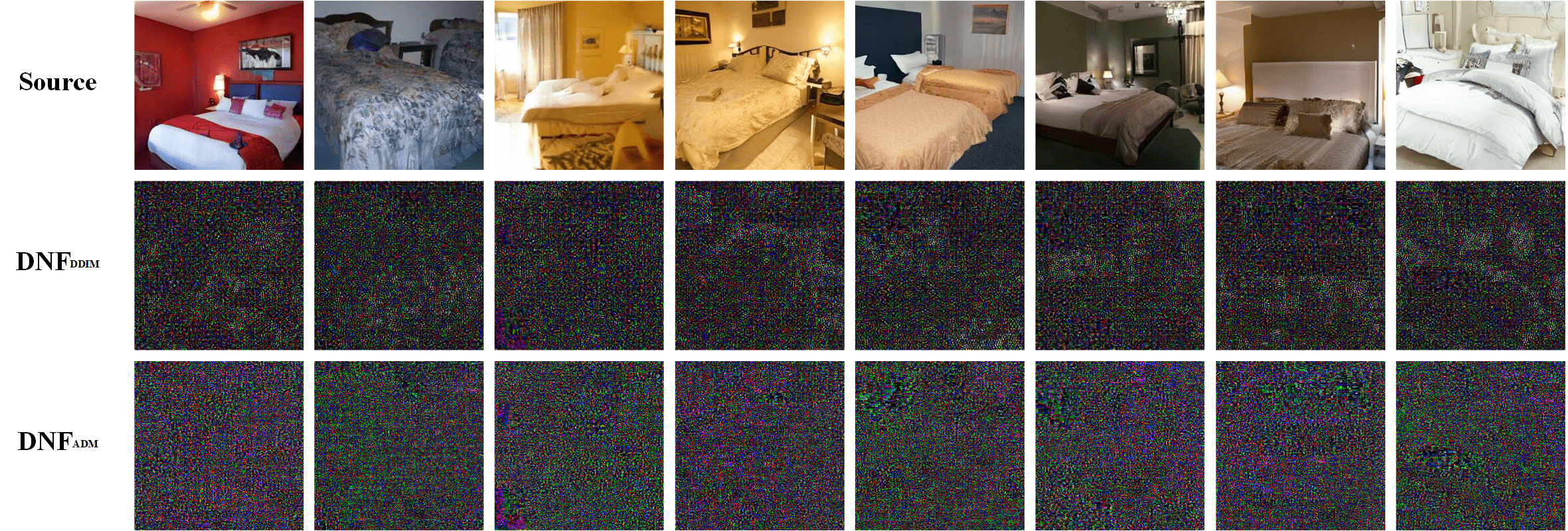
Figure 10: Visualization of DNF for fake images synthesized via DDPM [14].

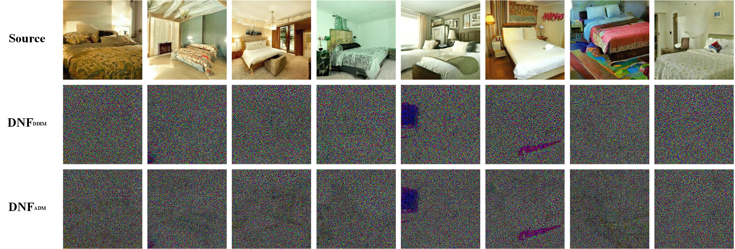
Figure 11: Visualization of DNF for fake images synthesized via PNDM [19].

Figure 12: Visualization of DNF for fake images synthesized via ADM [8].

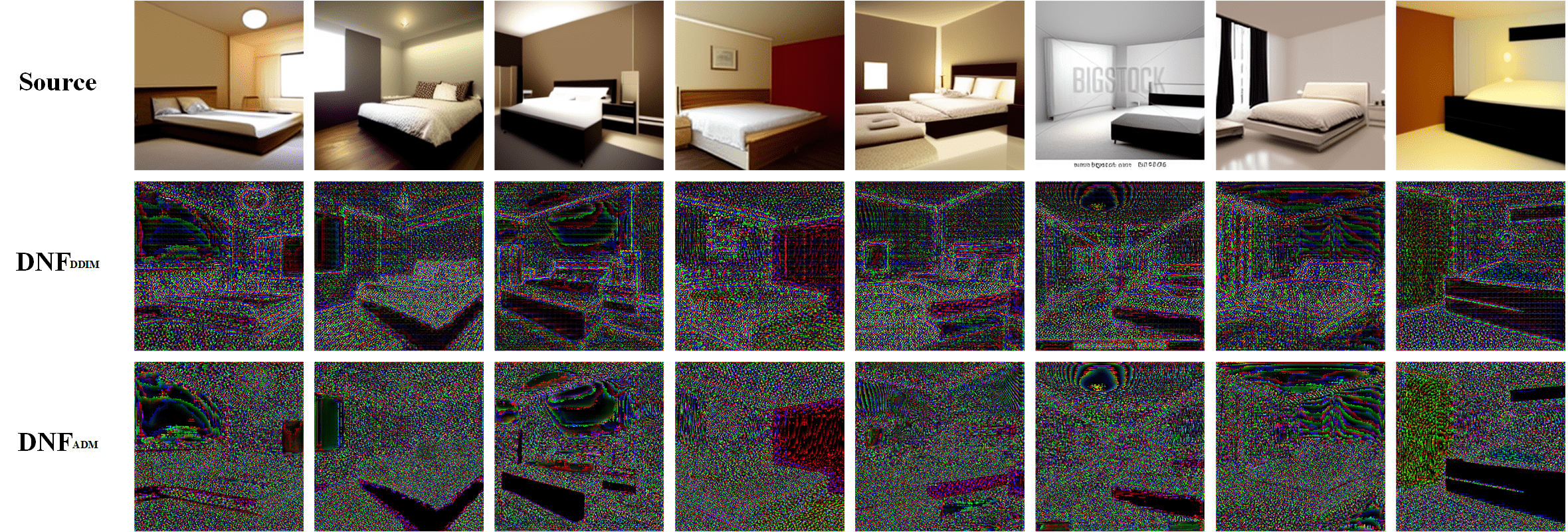
Figure 13: Visualization of DNF for fake images synthesized via LDM [27].

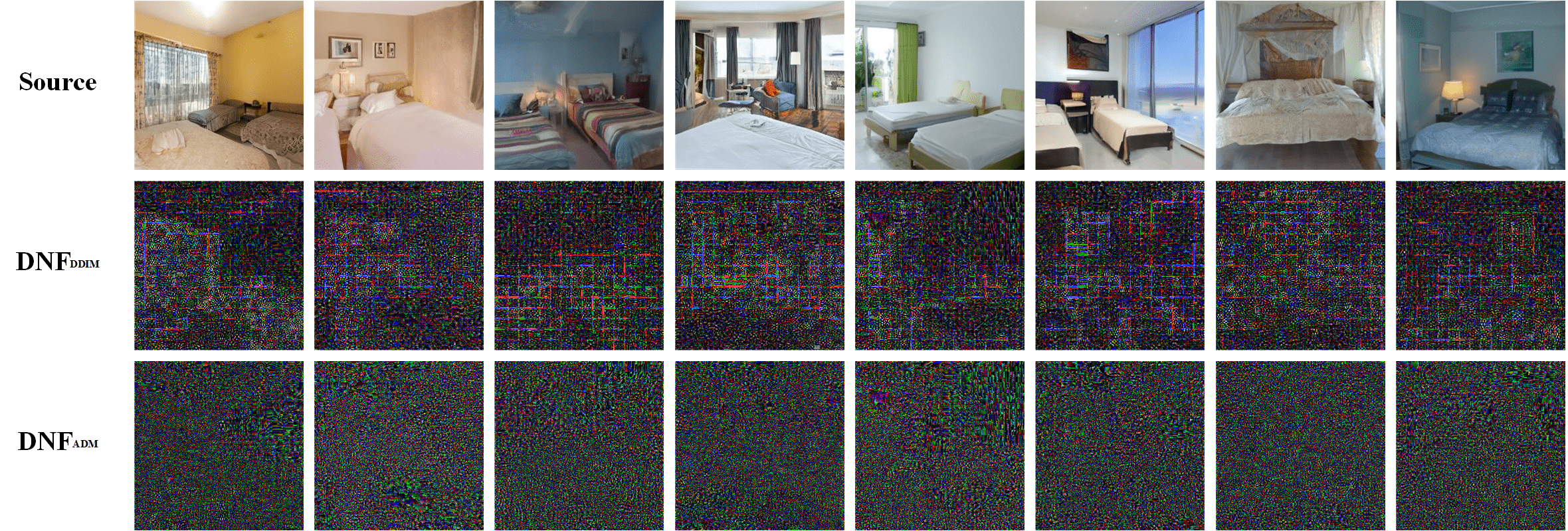
Figure 14: Visualization of DNF for fake images synthesized via iDDPM [23].

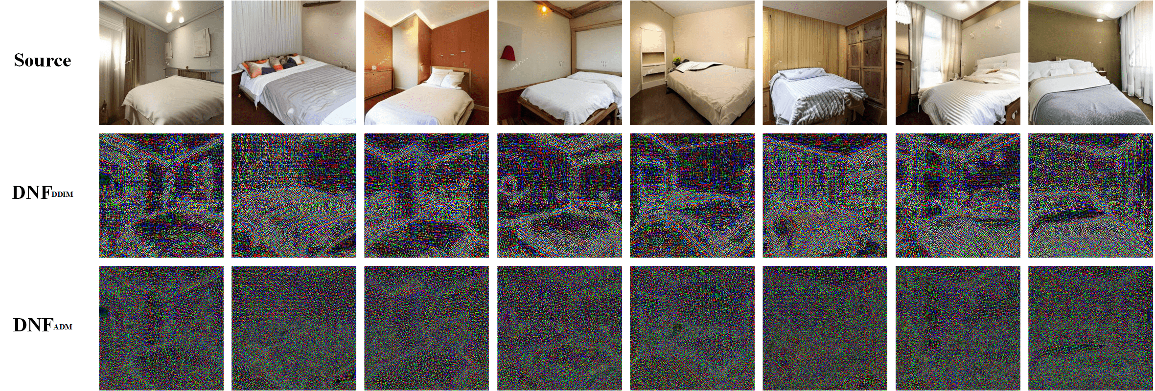
Figure 15: Visualization of DNF for fake images synthesized via VQ-Diffusion [13].

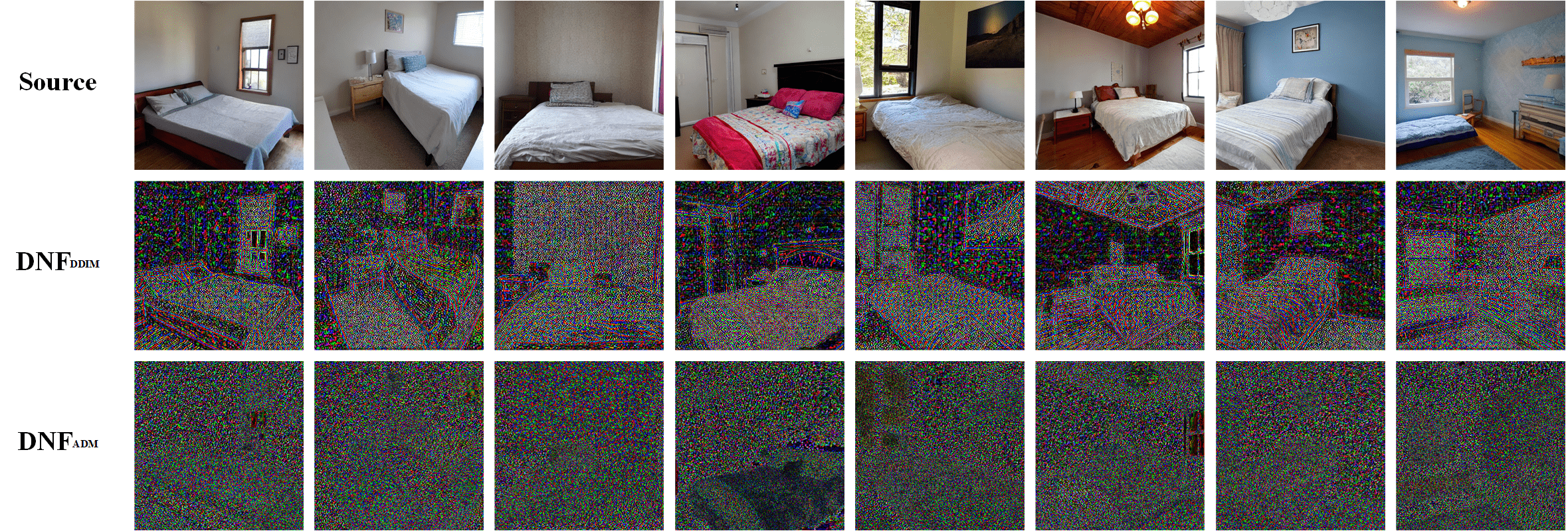
Figure 16: Visualization of DNF for fake images synthesized via Stable Diffusion v1 [27].

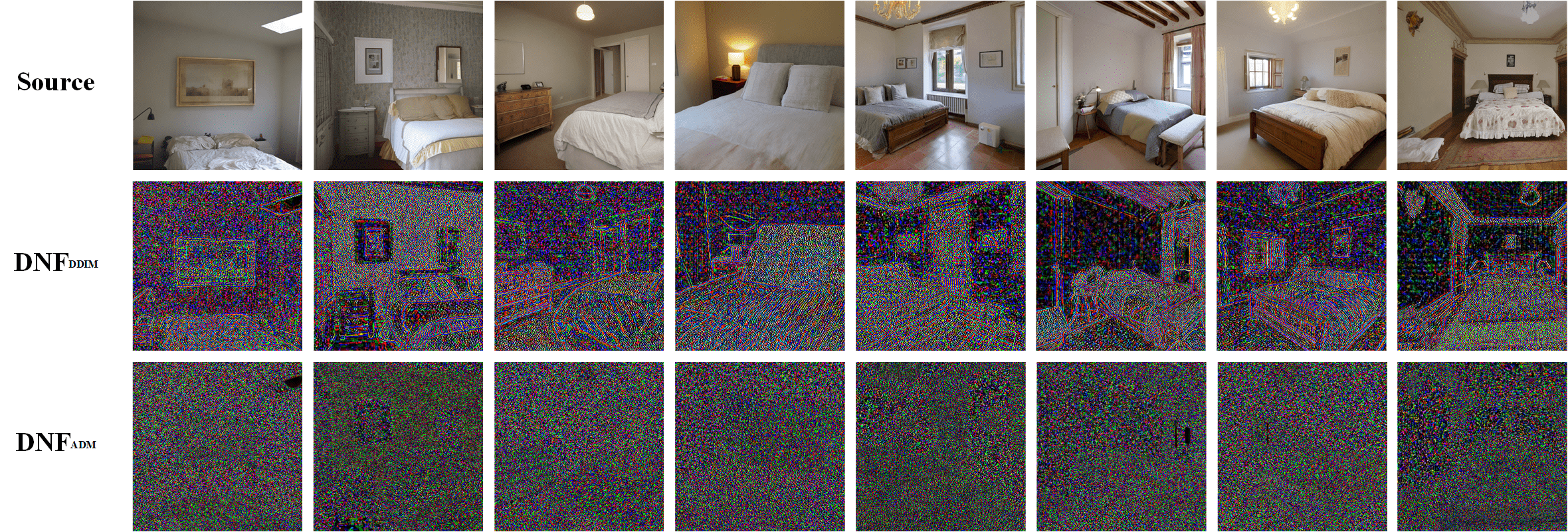
Figure 17: Visualization of DNF for fake images synthesized via Stable Diffusion v2 [27].

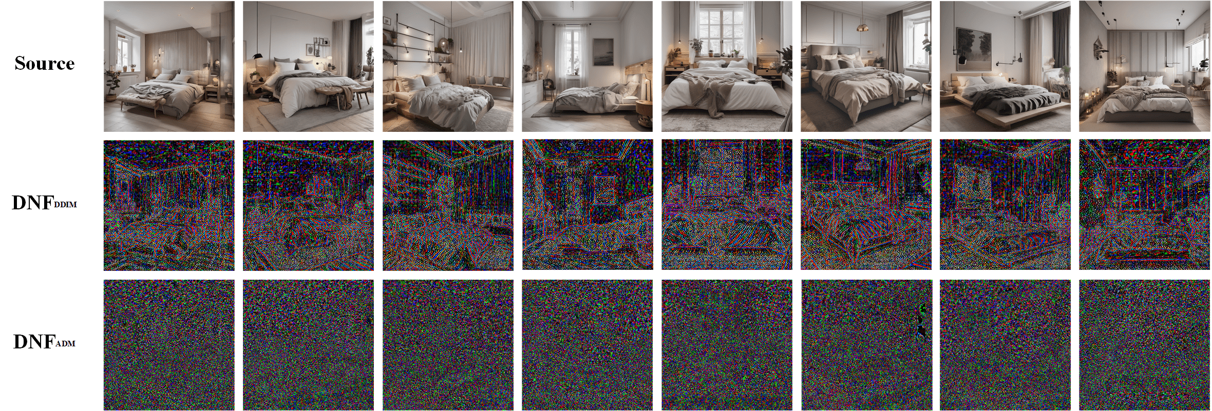
Figure 18: Visualization of DNF for fake images synthesized via Stable Diffusion XL [27].

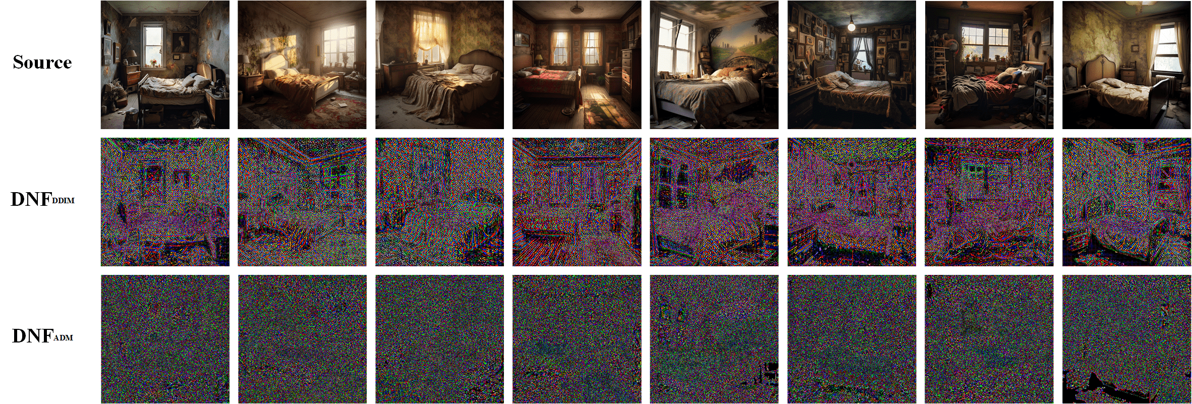
Figure 19: Visualization of DNF for fake images synthesized via Midjourney [21].

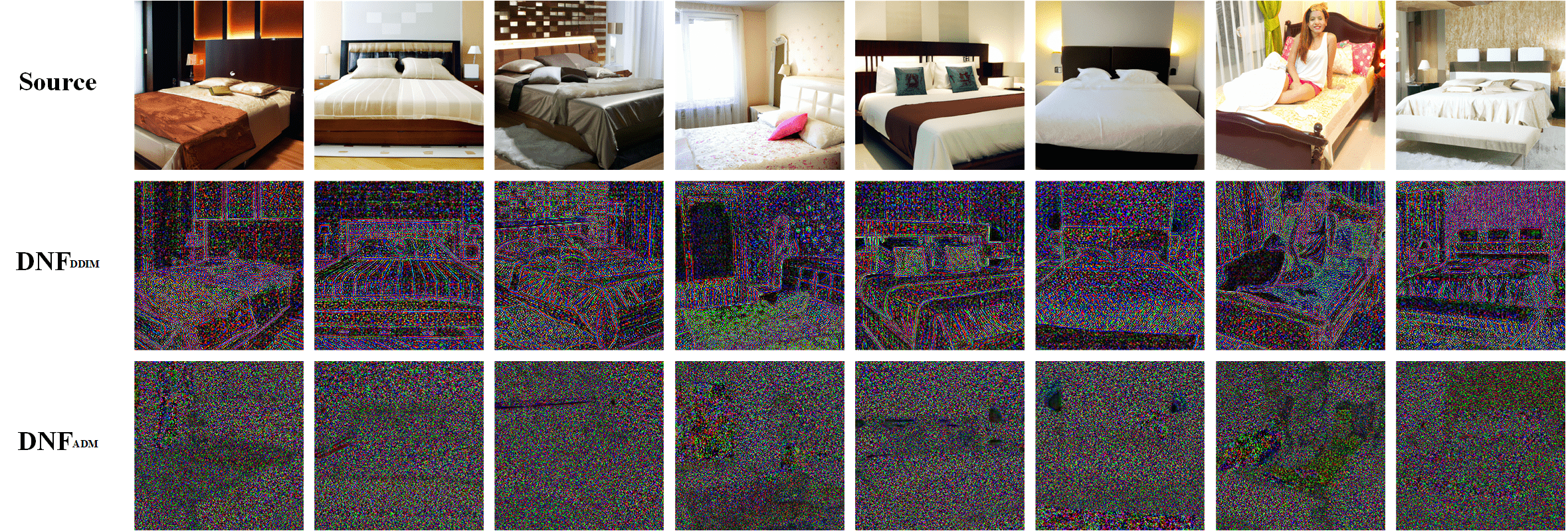
Figure 20: Visualization of DNF for fake images synthesized via DALL·E 2 [26].

References

- Brock et al. [2018] Andrew Brock, Jeff Donahue, and Karen Simonyan. Large scale gan training for high fidelity natural image synthesis. arXiv preprint arXiv:1809.11096, 2018.
- Cao et al. [2022] Junyi Cao, Chao Ma, Taiping Yao, Shen Chen, Shouhong Ding, and Xiaokang Yang. End-to-end reconstruction-classification learning for face forgery detection. In CVPR, 2022.
- Castillo et al. [2011] Carlos Castillo, Marcelo Mendoza, and Barbara Poblete. Information credibility on twitter. In Proceedings of the 20th international conference on World wide web, 2011.
- Chai et al. [2020] Lucy Chai, David Bau, Ser-Nam Lim, and Phillip Isola. What makes fake images detectable? understanding properties that generalize. In ECCV, 2020.
- Choi et al. [2018] Yunjey Choi, Minje Choi, Munyoung Kim, Jung-Woo Ha, Sunghun Kim, and Jaegul Choo. Stargan: Unified generative adversarial networks for multi-domain image-to-image translation. In CVPR, 2018.
- Corvi et al. [2023] Riccardo Corvi, Davide Cozzolino, Giada Zingarini, Giovanni Poggi, Koki Nagano, and Luisa Verdoliva. On the detection of synthetic images generated by diffusion models. In ICASSP, 2023.
- Deng et al. [2009] Jia Deng, Wei Dong, Richard Socher, Li-Jia Li, Kai Li, and Li Fei-Fei. Imagenet: A large-scale hierarchical image database. In CVPR, 2009.
- Dhariwal and Nichol [2021] Prafulla Dhariwal and Alexander Nichol. Diffusion models beat gans on image synthesis. NeurIPS, 2021.
- Fanelli [2009] Daniele Fanelli. How many scientists fabricate and falsify research? a systematic review and meta-analysis of survey data. PloS one, 2009.
- Frank et al. [2020] Joel Frank, Thorsten Eisenhofer, Lea Schönherr, Asja Fischer, Dorothea Kolossa, and Thorsten Holz. Leveraging frequency analysis for deep fake image recognition. In International conference on machine learning, 2020.
- Gedraite and Hadad [2011] Estevão S Gedraite and Murielle Hadad. Investigation on the effect of a gaussian blur in image filtering and segmentation. In Proceedings ELMAR-2011, 2011.
- Giglietto et al. [2019] Fabio Giglietto, Laura Iannelli, Augusto Valeriani, and Luca Rossi. ‘fake news’ is the invention of a liar: How false information circulates within the hybrid news system. Current sociology, 2019.
- Gu et al. [2022] Shuyang Gu, Dong Chen, Jianmin Bao, Fang Wen, Bo Zhang, Dongdong Chen, Lu Yuan, and Baining Guo. Vector quantized diffusion model for text-to-image synthesis. In CVPR, 2022.
- Ho et al. [2020] Jonathan Ho, Ajay Jain, and Pieter Abbeel. Denoising diffusion probabilistic models. NeurIPS, 2020.
- Karras et al. [2017] Tero Karras, Timo Aila, Samuli Laine, and Jaakko Lehtinen. Progressive growing of gans for improved quality, stability, and variation. arXiv preprint arXiv:1710.10196, 2017.
- Karras et al. [2019] Tero Karras, Samuli Laine, and Timo Aila. A style-based generator architecture for generative adversarial networks. In CVPR, 2019.
- Lau et al. [2003] W-L Lau, Z-L Li, and KW-K Lam. Effects of jpeg compression on image classification. International Journal of Remote Sensing, 2003.
- Li et al. [2023] Xiuyu Li, Yijiang Liu, Long Lian, Huanrui Yang, Zhen Dong, Daniel Kang, Shanghang Zhang, and Kurt Keutzer. Q-diffusion: Quantizing diffusion models. In ICCV, 2023.
- Liu et al. [2022] Luping Liu, Yi Ren, Zhijie Lin, and Zhou Zhao. Pseudo numerical methods for diffusion models on manifolds. arXiv preprint arXiv:2202.09778, 2022.
- Liu et al. [2018] Ziwei Liu, Ping Luo, Xiaogang Wang, and Xiaoou Tang. Large-scale celebfaces attributes (celeba) dataset. Retrieved August, 2018.
- Midjourney [2022] Midjourney. Midjourney. https://www.midjourney.com, 2022.
- Murdoch [2021] Blake Murdoch. Privacy and artificial intelligence: challenges for protecting health information in a new era. BMC Medical Ethics, 2021.
- Nichol and Dhariwal [2021] Alexander Quinn Nichol and Prafulla Dhariwal. Improved denoising diffusion probabilistic models. In ICML, 2021.
- Qi et al. [2019] Peng Qi, Juan Cao, Tianyun Yang, Junbo Guo, and Jintao Li. Exploiting multi-domain visual information for fake news detection. In 2019 IEEE international conference on data mining (ICDM), 2019.
- Qian et al. [2020] Yuyang Qian, Guojun Yin, Lu Sheng, Zixuan Chen, and Jing Shao. Thinking in frequency: Face forgery detection by mining frequency-aware clues. In ECCV, 2020.
- Ramesh et al. [2022] Aditya Ramesh, Prafulla Dhariwal, Alex Nichol, Casey Chu, and Mark Chen. Hierarchical text-conditional image generation with clip latents. arXiv, 2022.
- Rombach et al. [2022] Robin Rombach, Andreas Blattmann, Dominik Lorenz, Patrick Esser, and Björn Ommer. High-resolution image synthesis with latent diffusion models. In CVPR, 2022.
- Shi et al. [2023] Zenan Shi, Haipeng Chen, Long Chen, and Dong Zhang. Discrepancy-guided reconstruction learning for image forgery detection. arXiv preprint arXiv:2304.13349, 2023.
- Shiohara and Yamasaki [2022] Kaede Shiohara and Toshihiko Yamasaki. Detecting deepfakes with self-blended images. In CVPR, 2022.
- Song et al. [2020] Jiaming Song, Chenlin Meng, and Stefano Ermon. Denoising diffusion implicit models. arXiv preprint arXiv:2010.02502, 2020.
- Uyyala and Yadav [2023] Prabhakara Uyyala and Dyan Chandra Yadav. The advanced proprietary ai/ml solution as anti-fraudtensorlink4cheque (aftl4c) for cheque fraud detection. The International journal of analytical and experimental modal analysis, 2023.
- Wang et al. [2020] Sheng-Yu Wang, Oliver Wang, Richard Zhang, Andrew Owens, and Alexei A Efros. Cnn-generated images are surprisingly easy to spot… for now. In CVPR, 2020.
- Wang et al. [2023] Zhendong Wang, Jianmin Bao, Wengang Zhou, Weilun Wang, Hezhen Hu, Hong Chen, and Houqiang Li. Dire for diffusion-generated image detection. arXiv preprint arXiv:2303.09295, 2023.
- Yu et al. [2015] Fisher Yu, Ari Seff, Yinda Zhang, Shuran Song, Thomas Funkhouser, and Jianxiong Xiao. Lsun: Construction of a large-scale image dataset using deep learning with humans in the loop. arXiv preprint arXiv:1506.03365, 2015.
- Zhang et al. [2023] Lvmin Zhang, Anyi Rao, and Maneesh Agrawala. Adding conditional control to text-to-image diffusion models. In ICCV, 2023.
- Zhu et al. [2017] Jun-Yan Zhu, Taesung Park, Phillip Isola, and Alexei A Efros. Unpaired image-to-image translation using cycle-consistent adversarial networks. In ICCV, 2017.