Conductivity of concentrated salt solutions

Abstract

The conductivity of concentrated salt solutions has posed a real puzzle for theories of electrolytes. Despite a quantitative understanding of highly dilute solutions, an analytical theory for concentrated ones remains a challenge almost a century, although a number of parameters and effects incorporated into theories increases with time. Here we show that the conductivity of univalent salt solutions can be perfectly interpreted using an extremely simple model that relies just on a mean-field description of electrostatic effects and on an adapted for salt ions classical approach to calculating colloid electrophoresis. We derive a compact equation, which predicts that the ratio of conductivity at a finite concentration to that at an infinite dilution is the same for all salt, if it is plotted against a product of the harmonic mean of ion hydrodynamic radii and the square root of concentration. Our equation fits very well the experimental data for inorganic salts up to 3 mol/l.

The electrolyte solutions are ionic conductors, thanks to cations and anions formed as a result of dissociation. The electrical conductivity $K$ is one of their most important trait, which is widely used in chemical, biological as well as other applications, and the performance of many (e.g. energy storage) devices depends entirely on the ionic transport de Diego et al. (2001); Thirstrup and Deleebeeck (2021); Gu et al. (2023). The amount of water in Earth’s mantle is inferred from the conductivity data Yoshino and Katsura (2013). Besides, historically, the conductivity is the most important source of information on electrolyte properties (e.g. ion pairing) Marcus and Hefter (2006).

The physical origin of ionic conductivity is more or less clear. If an electric field $E$ is applied, ions migrate relative to a solvent by generating an electric current of density $J=KE$ (Ohm’s law). The migration speeds of ions are given by

$$V_{\pm}=M_{\pm}E,$$ (1)

where $M_{\pm}$ are their mobilities. The current densities induced in an univalent electrolyte are then $J_{\pm}=en_{\infty}V_{\pm}$, where $e$ is an elementary positive charge and $n_{\infty}=n_{\pm}$ is the number density (concentration) of an electrolyte solution. Consequently, the current density of a solution reads $J=J_{+}-J_{-}=eEn_{\infty}M,$ where $M=M_{+}-M_{-}$ is the difference in mobilities of cations and anions, and

$$K=en_{\infty}M$$ (2)

Thus, the calculations of the conductivity at a given concentration are reduced to those of $M$.

The quantitative understanding of ion mobilities is a challenging problem that has been addressed over nearly a century and by many groups, which is often termed a central issue of chemical physics Bernard et al. (2023); Naseri B. et al. (2023). The simplest expression can be derived by postulating the Stokes resistance to the ion propulsion

$$M_{\pm}\simeq M_{\pm}^{0}\simeq\pm\dfrac{e}{6\pi\eta R_{\pm}},$$ (3)

where $\eta$ is the dynamic viscosity of the solvent and $R_{\pm}$ are the hydrodynamic radii of the cation and anion. $M_{\pm}^{0}$ given by Eq.(3) and termed the mobilities at an infinite dilution do not depend on salt concentration. In this model

$$M\simeq M_{0}\simeq\dfrac{e}{3\pi\eta R_{h}}\,\mathrm{and}\,K\simeq K_{0}\simeq\dfrac{e^{2}n_{\infty}}{3\pi\eta R_{h}},$$ (4)

where $\eta$ is the dynamic viscosity of a solvent and $R_{h}=2(R_{+}R_{-})/(R_{+}+R_{-})$ is the harmonic mean of hydrodynamic radii. However, experiments on a conductivity show that $M$ and $K$ are generally smaller than predicted by (4) and this discrepancy augments on increasing salt concentration Kohlrausch (1900); de Diego et al. (2001). Chemists have long used this fact to infer a degree of dissociation (or an ion pairing). Physicists might view this simply as unreliability of hydrodynamic arguments based on the Stokes force.

One of the first systematic treatments of the influence of $n_{\infty}$ on conductivity was contained in a remarkable paper by Onsager (1927) who clarified a mechanism for the conductivity reduction, which involved electrophoresis and relaxation, and showed that the correction to $M_{0}$ depends on the square root of the concentration at a very high dilution. In efforts to better understand the connection between the ion mobilities and salt concentration many authors extended the theory, but failed to overcome a threshold of a few millimolars Fuoss (1978). However, most electrolyte solutions in nature and various applications are more concentrated. Thus, salt concentration in human blood plasma is about 0.15 mol/l, in the Atlantic Ocean it is $\simeq 0.6$ mol/l, Li-ion batteries and supercapacitor electrolytes are usually of concentration $1-2$ mol/l, reference electrolytes of pH-meters and glass micropipette electrodes - of concentration 3 mol/l.

Recent attempts to come to grips with the conductivity of concentrated solutions has been focused on a more sophisticated description of electrostatic and hydrodynamic contributions. Various techniques, such as the mean spherical approximation Dufrêche et al. (2005); Bernard et al. (2023), mode-coupling theory Chandra and Bagchi (1999); Aburto and Nägele (2013), density functional approach Chandra and Bagchi (1999); Avni et al. (2022), and more Goldsack et al. (1976); Villullas and Gonzalez (2005); Banerjee and Bagchi (2019); Naseri B. et al. (2023) have been employed. These publications involve additional parameters and effects, and mostly rely on numerical calculations. This makes them difficult to use and limits prediction capabilities.

In this Letter we suggest a completely different, simplified line to attack the conductivity problem. We present theoretical calculations for solutions composed of inorganic ions of unequal radius $R_{+}\neq R_{-}$, assuming that the conductivity takes its origin solely in an electrophoretic migration of ions. Our consideration is based on a recent theory of ionic electrophoresis that applies even at a very low dilution Vinogradova and Silkina (2023). We derive a simple conductivity equation and argue that relative conductivities, $K/K_{0}$, of all inorganic salts plotted against $R_{h}\sqrt{n_{\infty}}$ would collapse into a single curve. This conclusion is supported by providing a comparison with data for several standard salts, which shows that our theory is in excellent agreement with experiment up to concentrations of a few molars. While the relaxation is traditionally invoked in the conductivity theories, we demonstrate that this effect indeed affects a small decrement to a relative conductivity at very low concentrations, but does not play any role in concentrated solutions, where the reduction in conductivity becomes significant.

We consider a bulk 1:1 salt solution assuming that the description of its global static properties can be restricted to a mean-field Poisson-Boltzmann theory. The dimensionless electrostatic potential around each ion $\phi(z)=e\Phi(z)/(k_{B}T)$, where $k_{B}$ is the Boltzmann constant and $T$ is a temperature, represents a continuous function that depends on all other ions. The Debye screening length of a solution, $\lambda_{D}=\left(8\pi\ell_{B}n_{\infty}\right)^{-1/2}$, is defined as usually with the Bjerrum length, $\ell_{B}=\dfrac{e^{2}}{\varepsilon k_{B}T}$, where $\varepsilon$ is the solvent permittivity. By analyzing the experimental data it is more convenient to use the concentration $c_{\infty}[\rm{mol/l}]$, which is related to $n_{\infty}[\rm{m^{-3}}]$ as $n_{\infty}\simeq N_{A}\times 10^{3}\times c_{\infty}$, where $N_{A}$ is Avogadro’s number. The Bjerrum length of water at $T\simeq 298$ K is equal to about $0.7$ nm leading to a useful formula for 1:1 electrolyte

$$\lambda_{D}[\rm{nm}]\simeq\frac{0.305[\rm{nm}]}{\sqrt{c_{\infty}[\rm{mol/l}]}}$$ (5)

Thus upon increasing $c_{\infty}$ from $10^{-5}$ to $3$ mol/l the screening length is reduced from about 100 down to 0.18 nm.

We recall that the mean-field theory neglects correlations and finite sizes of ions and is traditionally assumed to be only accurate for dilute electrolytes. At concentrations above 0.5 mol/l this approach is normally considered as a first-order approximation only. Later we shall see that it is unlikely that all these alters the general features of the conductivity curve, but might introduce some (quite insignificant) quantitative changes.

Table 1: Some typical values of hydrodynamic radii of ions Kadhim and Gamaj (2020), they harmonic means and ratios.

Salt	$R_{+}$, nm	$R_{-}$, nm	$R_{h}$, nm	N
KBr	0.1295	0.1179	0.123	1.1
NaCl	0.184	0.1245	0.148	1.48
LiI	0.238	0.1135	0.154	2.1

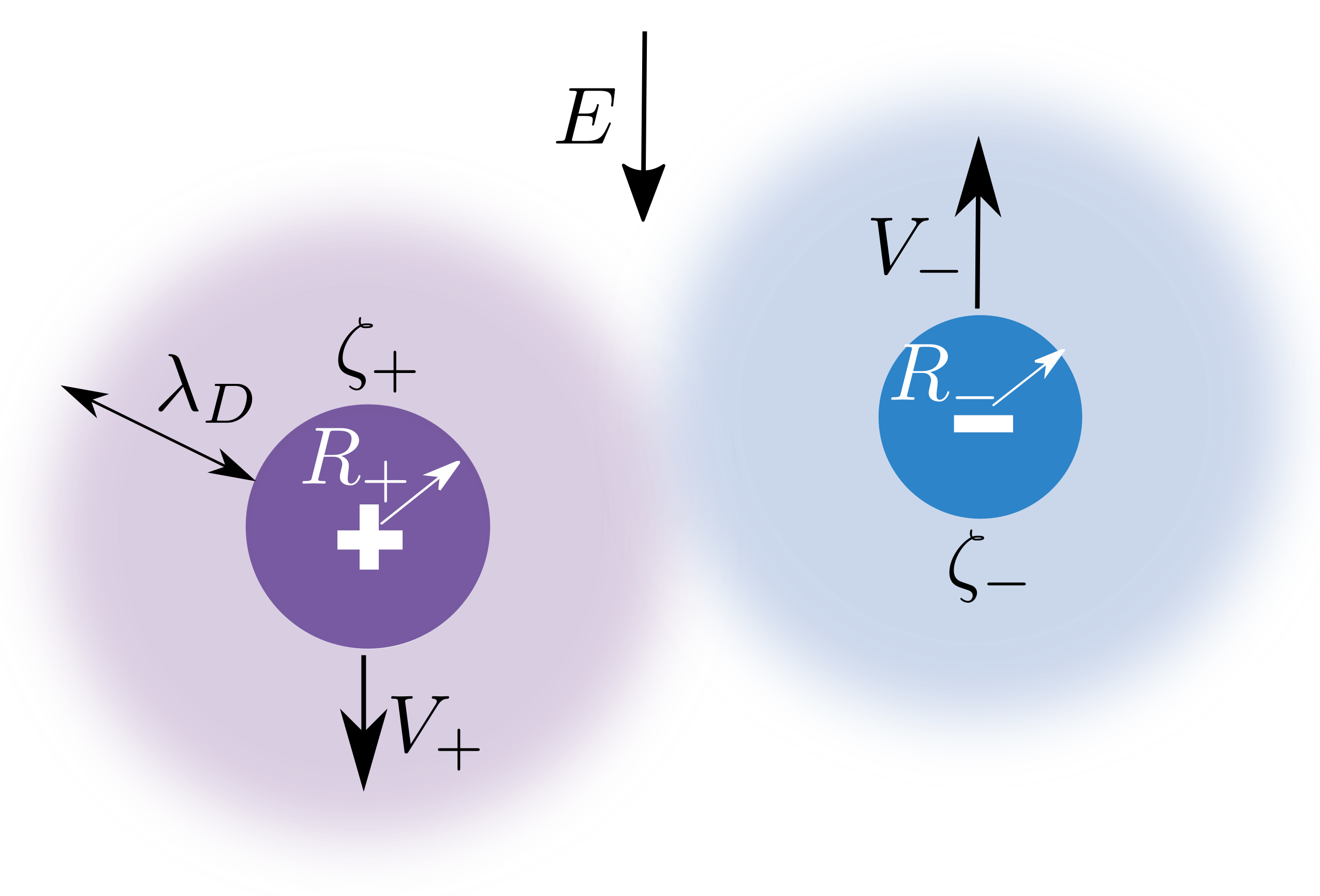
Figure 1: Sketch of the cation and anion with hydrodynamic radii $R_{+}$ and $R_{-}$ in the bulk electrolyte solution characterized by $\lambda_{D}$. The cation propels with the speed $V_{+}$ in the direction of the electric field $E$. Its zeta potential $\zeta_{+}$ (or dimensionless mobility) is positive. The anion of negative $\zeta_{-}$ migrates against the field with the velocity $V_{-}$.

By contrast, to describe the dynamic response to an external field, the ion hydrodynamic radii $R_{\pm}$ should be taken into account. Inorganic ions have a hydrodynamic radius from 0.1 to 0.3 nm Kadhim and Gamaj (2020), and we present the values for some univalent electrolytes in Table 1, together with $R_{h}$ and $N=R_{+}/R_{-}$. A sphere of radius $R_{\pm}$ with surface charge density $\pm e/(4\pi R_{\pm}^{2})$ would induce the same outer field as a point charge $\pm e$ located at its center. The surface potential $\phi_{s\pm}$ is established self-consistently and salt-dependent. Close to the ions the electrostatic diffuse layers (EDLs) are formed, which extension is defined by $\lambda_{D}$. So, it is convenient to introduce the dimensionless radii of ions $\varrho_{\pm}=R_{\pm}/\lambda_{D}$. Note that in the range of $c_{\infty}$ below 3 mol/l we consider here, the values of $\varrho_{\pm}$ remain smaller than unity or very close to it. Say, if we set $c_{\infty}=2$ mol/l, then for a largest ion (Li⁺) in Table 1 we obtain $\varrho_{+}\simeq 1$, but for a smallest (I^-) we get $\varrho_{-}\simeq 0.5$.

When an electric field $E$ is applied, an electro-osmotic flow around such spheres of unit charge is induced. The electroosmosis takes its origin in the EDL, where a tangential electric field generates a force that sets the fluid in motion. The emergence of this flow in turn provides hydrodynamic stresses that cause the propulsion of the ions with a velocity given by Eq.(1) as sketched in Fig. 1. Since the field is weak, we suppose that EDLs are not deformed and the relaxation effect is absent. We return to the importance of the relaxation later, by focusing now on electrophoresis solely. Ion mobilities are defined as

$$M_{\pm}=\dfrac{\varepsilon Z_{\pm}}{4\pi\eta}=\dfrac{e}{4\pi\eta\ell_{B}}\zeta_{\pm},$$ (6)

where $Z_{\pm}$ are the electrokinetic or zeta potentials of cations and anions, which appears in (6) via the Stokes equation, and $\zeta_{\pm}=eZ_{\pm}/k_{B}T$ are the dimensionless zeta potentials.

Zeta potentials of small inorganic ions are given by Vinogradova and Silkina (2023)

$$\zeta_{\pm}\simeq\phi_{s\pm}\mathcal{F_{\pm}}\simeq\pm\dfrac{\ell_{B}}{R_{\pm}(1+\varrho_{\pm})}\mathcal{F_{\pm}},$$ (7)

where $\mathcal{F_{\pm}}$ are the special functions derived by Henry Henry (1931)

$$\mathcal{F_{\pm}}=1-e^{\varrho_{\pm}}\left[5\operatorname{Ei}_{7}(\varrho_{\pm})-2\operatorname{Ei}_{5}(\varrho_{\pm})\right],$$ (8)

where $\operatorname{Ei}_{p}(\varrho_{\pm})=\varrho_{\pm}^{p-1}\Gamma(1-p,\varrho_{\pm})=\varrho_{\pm}^{p-1}\int_{\rho}^{\infty}\frac{e^{-t}}{t^{p}}dt$ are the generalized exponential integrals. Since for inorganic ions $\varrho_{\pm}$ does not exceed unity, Eq. (8) can be reduced to

$$\mathcal{F_{\pm}}\simeq\dfrac{2}{3}\left[1+\left(\dfrac{\varrho_{\pm}}{4}\right)^{2}\right]$$ (9)

Substituting then (9) into Eq.(7) and expanding about $\varrho=0$ one can obtain

$$\zeta_{\pm}\simeq\pm\dfrac{2\ell_{B}}{3R_{\pm}}\left[1-\varrho_{\pm}+17\left(\dfrac{\varrho_{\pm}}{4}\right)^{2}\left(1+\sum_{k=1}^{\infty}(-\varrho_{\pm})^{k}\right)\right]$$

The last equation is converged to

$$\zeta_{\pm}\simeq\pm\dfrac{2\ell_{B}}{3R_{\pm}}\left[1-\varrho_{\pm}+17\dfrac{\left(\dfrac{\varrho_{\pm}}{4}\right)^{2}}{1+\varrho_{\pm}}\right]$$ (10)

Clearly, the upper bound for the zeta potential is attained when $\rho_{\pm}\to 0$ (an infinite dilution)

$$\zeta_{\pm}\to\zeta_{0\pm}\simeq\pm\dfrac{2\ell_{B}}{3R_{\pm}}.$$ (11)

Figure 2: Zeta potentials $\zeta_{\pm}$ computed for K⁺, Li⁺, Cl^-, I^- (solid curves from top to bottom). Dashed lines are obtained using Eq. (11). Symbols show calculations from Eq. (10).

Figure 2 includes computed zeta potentials of several ions. For these examples we take from Table 1 cations (K⁺, Li⁺) and anions (I^-, Cl^-) of smallest and largest radius. Calculations are made using the first equality in (7) with $\phi_{s\pm}$ found numerically from the nonlinear Poisson-Boltzmann equation and $\mathcal{F_{\pm}}$ calculated from Eq. (8). The straight lines corresponding to $\zeta_{0\pm}$ given by (11) describe perfectly the distinct plateau regions at very low concentrations. On increasing concentration, however, the absolute values of $\zeta_{\pm}$ decrease. Also included are calculations from (Conductivity of concentrated salt solutions). It can be seen that their fit to numerical data is extremely good in the whole concentration range.

From Eq.(6) it follows that

$$M\simeq\dfrac{e}{4\pi\eta\ell_{B}}(\zeta^{+}-\zeta^{-})$$ (12)

Substituting (10) and performing standard calculations we derive

$$\dfrac{M}{M_{0}}\equiv\dfrac{K}{K_{0}}\simeq 1-\varrho_{h}+\dfrac{17}{32}\varrho_{h}\left(\dfrac{\varrho_{+}}{1+\varrho_{+}}+\dfrac{\varrho_{+}}{N+\varrho_{+}}\right),$$ (13)

where $M_{0}$ and $K_{0}$ are given by Eqs.(4) and $\varrho_{h}=R_{h}/\lambda_{D}=2\varrho_{+}/(1+N)$. Figure 3 shows $K/K_{0}$ calculated from Eq.(13) as a function of $c_{\infty}$. The calculations are compared with experimental data for three standard salts Vanýsek (2000). As seen from Table 1, for these examples $N$ varies from 1.1 for KBr, but can be larger than 2 (e.g. for LiI). An overall conclusion from this linear scale plot is that the theoretical curve for $K/K_{0}$ is well consistent with experiment. At large concentrations Eq.(13) predicts either slightly lower (KBr) or higher (NaCl) conductivities, but still fits data quite well. This is a startling result since our theory omits a few nonidealities, which are normally considered to be important at high salt (i.e. 0.5-3 mol/l).

Figure 3: $K_{\infty}/K_{\infty}^{0}$ as a function of $c_{\infty}$ for KBr, NaCl and LiI aqueous solution calculated from Eqs. (13) and (14) (solid and dashed curves). Open and filled circles indicate experimental data from Vanýsek (2000) and Miller (1966), open and filled squares show data from Dobos (1975) and Lobo (1984).

When $N=1$, we get $\varrho_{h}=\varrho_{+}$ and (13) reduces to

$$\dfrac{K}{K_{0}}\simeq 1-\varrho_{h}\left(1-\dfrac{17}{16}\dfrac{\varrho_{h}}{1+\varrho_{h}}\right)$$ (14)

The calculation from Eq.(14) is also included in Fig. 3. It can be seen that deviations from Eq. (13) are extremely small. To examine their significance more closely, we now calculate the difference between (13) and (14)

$$\Delta=\dfrac{17}{32}\varrho_{h}\left(\dfrac{\varrho_{+}}{1+\varrho_{+}}+\dfrac{\varrho_{+}}{N+\varrho_{+}}-\dfrac{4\varrho_{+}}{1+N+2\varrho_{+}}\right)$$ (15)

The calculations show that $\Delta\geq 0$, and is always below a couple of %. We thus conclude that compact approximate Eq. (14), which is easy to handle, can safely be employed to interpret data for inorganic salts or for a predictive purpose.

It follows from (5) that $\varrho_{h}\simeq 3.379R_{h}\sqrt{c_{\infty}}$ for a fixed $T=298$ K, where $R_{h}$ should be taken in nm. This implies that the values of $K/K_{0}$ for any univalent salt solution plotted against (dimensionless) $R_{h}\sqrt{c_{\infty}}$ should collapse into a single curve. That this is indeed so is demonstrated in Fig. 4, where we plot in a semi-log scale a relative conductivity calculated from (14) vs. $R_{h}\sqrt{c_{\infty}}$ along with the experimental data for a variety of inorganic salts at $T=298$K Vanýsek (2000); Dobos (1975); Lobo (1984); Shedlovsky (1932); Miller (1966). Besides salts presented in Table 1 we include KCl, LiCl, and LiClO₄ using their $R_{h}$ = 0.127, 0.163, and 0.174 nm, correspondingly, to re-scale the concentration. Note that since the theory is justified provided $R_{h}\sqrt{c_{\infty}}$ is below ca. 0.305, we employ for this plot only data for $c_{\infty}\leq 3$ mol/l. One can see that the approximate theory is in a good agreement with the data for all salts, perhaps with only insignificant discrepancy at low dilution that is probably comparable with the experimental error. The discrepancy is always in the direction of smaller $K/K_{0}$ than predicted by Eq. (14), but the data for KBr and KCl show slightly larger $K/K_{0}$. The reason for qualitative differences only for these two salts is unclear. The relaxation, if any, could only reduce $K$, so one can speculate that we deal with an ionic specificity Salis and Ninham (2014), but this has to be explored. For $\varrho_{h}\ll 1$, Eq. (14) reduces to the Onsager formula for the electrophoretic effect

$$\dfrac{K}{K_{0}}\simeq 1-\varrho_{h}$$ (16)

The curve calculated from Eq. (16) is also included in Fig. 4. Clearly, the data obtained at high salt are irreconcilable with this linear equation.

Figure 4: $K/K_{0}$ as a function of $R_{h}\sqrt{c_{\infty}}$ plotted in a semi-log scale (solid curve) and experimental data for standards salts taken from Refs. Vanýsek (2000); Dobos (1975); Lobo (1984); Shedlovsky (1932); Miller (1966) shown by filled symbols. Dashed curve corresponds to calculations from Eq. (16).

Figure 5: A decrement to a relative conductivity, $1-K/K_{0}$, plotted against $R_{h}\sqrt{c_{\infty}}$ in a log-log scale (solid curve). Symbols show the same data as in Fig. 4. Dashed and dotted lines are calculated from Eqs. (16) and (17).

To examine the discrepancy from data more closely, the results for salts from Fig. 4 are reproduced in Fig. 5, where a decrement to a relative conductivity, $1-K/K_{0}$, is plotted against $R_{h}\sqrt{c_{\infty}}$ in a log-log scale. It can be seen that in highly dilute solutions the data are slightly above the theory. An explanation can be obtained if we invoke the relaxation effect Onsager (1927). In our notations this yields

$$\dfrac{K}{K_{0}}\simeq 1-\varrho_{h}\left[1+\frac{1}{3}\left(1-\frac{1}{\sqrt{2}}\right)\frac{\ell_{B}}{R_{h}}\right],$$ (17)

but note that this expression is justified only when $\varrho_{h}\ll 1$. Indeed, Eq. (17) provides an excellent fit to the data up to $R_{h}\sqrt{c_{\infty}}\simeq 6\times 10^{-3}$ (millimolar concentrations). Note the since the relaxation is ion specific here for calculations we used $R_{h}$ for KCl. Upon increasing concentration further the experimental data begin to approach to calculations from the theory accounting solely the electrophoretic effect, and in concentrated solutions, $R_{h}\sqrt{c_{\infty}}\geq 8\times 10^{-2}$ (or $c_{\infty}\geq 0.5$ mol/l), our theory is in a very good agreement with experiment. It is natural to speculate that the relaxation effect reduces with $c_{\infty}$ and disappears at high concentrations. We also remark that although the relaxation indeed slightly retards the migration of ions in highly dilute solutions, in this case the decrease in conductivity is very small.

In summary, Eq. (14) describes very well a master conductivity curve valid for all univalent salts at any concentration up to 3 mol/l or so. It appears, of course, surprising that such a compact equation, and we have clearly oversimplified in presenting the case, works very well in so large concentration range and for all salts, but the conclusions are unambiguous:

• The conductivity of salt solutions is dictated mainly by ionic electrophoresis. Whether or not some, essentially very small, deviations are due to correlations, relaxation or other effects is in fact irrelevant for most of the applications;

• The electrophoresis of inorganic ions can be accommodated within a theoretical framework that relies solely on a standard mean-field description of electrostatics and admits only a harmonic mean of hydrodynamic radii in describing ionic migration. The need to invoke specific constants as (arbitrary) parameters, or to correct an ionic concentration is thereby removed.

This bears on the whole question of what we mean by a degree of dissociation that is often inferred from the conductivity measurements not . Our results show that the conductivity is interpreted without invoking the formation of ionic pairs, thus supporting the notion of complete dissociation of strong electrolytes. However remote from mainstream thinking this conclusion may seem, it would be worthwhile to recall that there are still lingering doubts about the reality of ion pairing, at least for univalent electrolytes in high permittivity solvents Marcus and Hefter (2006); Zavitsas (2001).

Our considerations can be extended to asymmetric multivalent salts. The same concerns the temperature dependence of $K$, which follows from our theory, but requires the validation in terms of fit to experimental results. Another fruitful direction could be to consider the salt-dependence of a mobility of adsorbed ions Maduar et al. (2015); Mouterde and Bocquet (2018), which impacts hydrophobic electrokinetics Vinogradova et al. (2023).

This research was supported by the Ministry of Science and Higher Education of the Russian Federation.

References

- de Diego et al. (2001) A. de Diego, A. Usobiaga, L. A. Fernández, and J. M. Madariaga, TrAc trends in analytical chemistry 20, 65 (2001).
- Thirstrup and Deleebeeck (2021) C. Thirstrup and L. Deleebeeck, IEEE Trans. Instrum. Meas. 70, 1 (2021).
- Gu et al. (2023) Y. Gu, X. Qi, X. Yang, Y. Jiang, P. Liu, X. Quan, and P. Liang, Water Research , 119630 (2023).
- Yoshino and Katsura (2013) T. Yoshino and T. Katsura, Annu. Rev. Earth Planet Sci. 41, 605 (2013).
- Marcus and Hefter (2006) Y. Marcus and G. Hefter, Chem. Rev. 106, 4585 (2006).
- Bernard et al. (2023) O. Bernard, M. Jardat, B. Rotenberg, and P. Illien, J. Chem. Phys. 159, 164105 (2023).
- Naseri B. et al. (2023) S. Naseri B., B. Maribo-Mogensen, X. Liang, and G. M. Kontogeorgis, J. Phys. Chem. B 127, 9954 (2023).
- Kohlrausch (1900) F. Kohlrausch, Ann. Phys. 306, 132 (1900).
- Onsager (1927) L. Onsager, Phys. Z. 28, 277 (1927).
- Fuoss (1978) R. M. Fuoss, J. Solution Chem. 7, 771 (1978).
- Dufrêche et al. (2005) J.-F. Dufrêche, O. Bernard, S. Durand-Vidal, and P. Turq, J. Phys. Chem. B 109, 9873 (2005).
- Chandra and Bagchi (1999) A. Chandra and B. Bagchi, J. Chem. Phys. 110, 10024 (1999).
- Aburto and Nägele (2013) C. C. Aburto and G. Nägele, J. Chem. Phys. 139 (2013).
- Avni et al. (2022) Y. Avni, R. M. Adar, D. Andelman, and H. Orland, Phys. Rev. Lett. 128, 098002 (2022).
- Goldsack et al. (1976) D. E. Goldsack, R. Franchetto, and A. Franchetto, Can. J. Chem. 54, 2953 (1976).
- Villullas and Gonzalez (2005) H. M. Villullas and E. R. Gonzalez, J. Phys. Chem. B 109, 9166 (2005).
- Banerjee and Bagchi (2019) P. Banerjee and B. Bagchi, J. Chem. Phys. 150 (2019).
- Vinogradova and Silkina (2023) O. I. Vinogradova and E. F. Silkina, J. Chem. Phys. 159, 174707 (2023).
- Kadhim and Gamaj (2020) M. J. Kadhim and M. I. Gamaj, J. Chem. Rev. 2, 182 (2020).
- Henry (1931) D. C. Henry, Proc. R. Soc. Lond. Ser. A 133, 106 (1931).
- Vanýsek (2000) P. Vanýsek, CRC Handbook of Chemistry and Physics 8, 8 (2000).
- Miller (1966) D. G. Miller, J. Phys. Chem. 70, 2639 (1966).
- Dobos (1975) D. Dobos, Electrochemical data. A handbook for electrochemists in industry and universities (Akademiai Kiado, 1975).
- Lobo (1984) V. M. M. Lobo, Electrolyte solutions: Literature data on thermodynamic and transport properties, Vol. II (Coimbra Editora, 1984).
- Shedlovsky (1932) T. Shedlovsky, J. Amer. Chem. Soc. 54, 1411 (1932).
- Salis and Ninham (2014) A. Salis and B. W. Ninham, Chem. Soc. Rev. 43, 7358 (2014).
- (27) Dielectric relaxation Buchner (2008) that also provides some evidences of ion pairing is very sensitive to the conductivity contribution that becomes dominant at low frequencies and should be properly accounted.
- Zavitsas (2001) A. A. Zavitsas, J. Phys. Chem. B 105, 7805 (2001).
- Maduar et al. (2015) S. R. Maduar, A. V. Belyaev, V. Lobaskin, and O. I. Vinogradova, Phys. Rev. Lett. 114, 118301 (2015).
- Mouterde and Bocquet (2018) T. Mouterde and L. Bocquet, Eur. Phys. J. E 41, 148 (2018).
- Vinogradova et al. (2023) O. I. Vinogradova, E. F. Silkina, and E. S. Asmolov, Curr. Opin. Colloid Interface Sci. 68, 101742 (2023).
- Buchner (2008) R. Buchner, Pure Appl. Chem. 80, 1239 (2008).