Quasi-isomorphism of grid chain complexes for a connected sum of knots

Abstract.

We give a purely combinatorial proof of the Künneth formula for the knot Floer homology of connected sums by constructing a quasi-isomorphism of grid chain complexes. This proof is complete within the framework of the knot grid homology. The construction of the quasi-isomorphism naturally deduces that the Legendrian and transverse invariants behave functorially with respect to the connected sum operation.

1. Introduction

Grid homology is a combinatorial reconstruction of knot Floer homology developed by Manolescu, Ozsváth, Szabó, and Thurston [10]. Because grid homology is a purely combinatorial theory without holomorphic theory, it is an interesting problem whether the known results of knot Floer homology can be shown in the framework of grid homology. For example, there are combinatorial reformulations of the knot Floer invariants such as the tau, epsilon, and Upsilon invariant [14, 6, 4]. Furthermore, the tau and Upsilon invariants were combinatorially proved to be concordance invariants in [15, 7], respectively.

In this paper, we only consider knots in $S^{3}$ and discuss the hat version of grid homology and knot Floer homology. There is the Künneth formula for the knot Floer homology of connected sums

(1.1) $$\widehat{HFK}(K_{1})\otimes\widehat{HFK}(K_{2})\cong\widehat{HFK}(K_{1}\#K_{2}).$$

In [8], the author proved (1.1) by applying the grid homology for spatial graphs. However, we proved the existence of the isomorphism of the homologies without the concrete isomorphism. We verified this by observing the tilde chain complexes that are reduced complexes of the hat complexes depending on grid diagrams. In addition, the proof needs the extended grid homology for spatial graphs and is not completed within the framework of the knot grid homology.

The former result of the present paper is a refinement of the work in [8]. We explore the hat version of grid chain complexes to give quasi-isomorphism of the formula.

Theorem 1.1.

Let $g_{1}$ and $g_{2}$ be two good (Definition 4.1) grid diagrams representing two knots $K_{1}$ and $K_{2}$ respectively. Let $g_{\#}$ be the grid diagram representing $K_{1}\#K_{2}$ obtained by $g_{1}$ and $g_{2}$. Then there is a quasi-isomorphism

$$\widehat{GC}(g_{1})\otimes\widehat{GC}(g_{2})\to\widehat{GC}(g_{\#}).$$

Remark 1.2.

Every knot is represented by a good grid diagram. The proof of this theorem is complete within the framework of the knot grid homology.

Grid homology gives effective invariants for Legendrian and transverse knots in $(\mathrm{R}^{3},\xi_{\mathrm{std}})$ [12]. For example, two Legendrian knots with the topological type $5_{2}$ and the same classical invariants are distinguished by the grid Legendrian invariant [2, 12]. This invariant is known to provide obstructions to decomposable Lagrangian cobordisms, certain good cobordisms between two Legendrian knots [1, Theorem 1.2]. The grid transverse invariant is applied to study the transverse simplicity of topological knots [11]. These invariants are extended to null-homologous Legendrian and transverse knots in general closed contact three-manifolds [9].

The grid Legendrian invariants are defined to be the homology classes determined by the canonical generators of the chain complex. By the construction of the quasi-isomorphism of the above theorem, we can easily trace the generators, so we can quickly show the following$\colon$

Theorem 1.3.

Let $g_{1}$ and $g_{2}$ be two good (Definition 4.1) grid diagrams representing two Legendrian knots $\mathcal{K}_{1}$ and $\mathcal{K}_{2}$ respectively. Let $g_{\#}$ be the grid diagram representing $\mathcal{K}_{1}\#\mathcal{K}_{2}$ obtained by $g_{1}$ and $g_{2}$. Then there is a quasi-isomorphism

$$\widehat{GC}(g_{1})\otimes\widehat{GC}(g_{2})\to\widehat{GC}(g_{\#})$$

which maps $\widehat{\lambda}_{+}(\mathcal{K}_{1})\otimes\widehat{\lambda}_{+}(\mathcal{K}_{2})$ to $\widehat{\lambda}_{+}(\mathcal{K}_{1}\#\mathcal{K}_{2})$ and $\widehat{\lambda}_{-}(\mathcal{K}_{1})\otimes\widehat{\lambda}_{-}(\mathcal{K}_{2})$ to $\widehat{\lambda}_{-}(\mathcal{K}_{1}\#\mathcal{K}_{2})$.

The grid transverse invariant is defined to be the homology class $\widehat{\lambda}_{+}\in\widehat{GH}(g)$, so the following corollary is proved immediately.

Corollary 1.4.

Let $g_{1}$ and $g_{2}$ be two good grid diagrams representing the transverse knots $\mathcal{T}_{1}$ and $\mathcal{T}_{2}$ respectively. Let $g_{\#}$ be the grid diagram representing $\mathcal{T}_{1}\#\mathcal{T}_{2}$ obtained by $g_{1}$ and $g_{2}$. Then there is a quasi-isomorphism

$$\widehat{GC}(g_{1})\otimes\widehat{GC}(g_{2})\to\widehat{GC}(g_{\#})$$

which maps $\widehat{\theta}(\mathcal{T}_{1})\otimes\widehat{\theta}(\mathcal{T}_{2})$ to $\widehat{\theta}(\mathcal{T}_{1}\#\mathcal{T}_{2})$.

These are purely combinatorial proofs of Vétesi’s results [16, Corollaries 1.2 and 1.3].

1.1. Outline of the paper.

In Section 2, we review the knot grid homology. In Section 3, we briefly describe Legendrian and transverse knots and the relation between them to grid homology. In Section 4, we prepare some notations and define useful chain complexes to prove the main theorem. In section 5, we give the construction of a quasi-isomorphism and prove the main theorem.

2. The definition of grid homology for knots

This section quickly provides an overview of grid homology for knots and links. Referring to [13, Remark 4.6.13], we will introduce the hat version without using the minus version. See [13] for details.

A planar grid diagram $g$ (Figure 1) is an $n\times n$ grid of squares some of which is decorated with an $X$- or $O$- marking such that it satisfies the following conditions.

1. There is exactly one $O$ and $X$ on each row and column.

2. $O$’s and $X$’s do not share the same square.

We denote the set of $O$- by $\mathbb{O}$ and the set of $X$-markings by $\mathbb{X}$. We often use the labeling of markings as $\{O_{i}\}_{i=1}^{n}$ and $\{X_{j}\}_{j=1}^{m}$.

A grid diagram determines a link in $S^{3}$. Drawing oriented segments from the $O$-markings to the $X$-markings in each row and oriented segments from the $X$-markings to the $O$-marking in each column. Assume that the vertical segments always cross above the horizontal segments. Then we can recover the link diagram. In this paper, we only consider grid diagrams representing knots.

It is known that any two grid diagrams for the same knot can be connected by a finite sequence of moves on grid diagrams called grid moves; see [3, 10].

A toroidal grid diagram is a grid diagram that is regarded as a diagram on the torus obtained by identifying edges in a natural way. We assume that every toroidal diagram is oriented in a natural way. We write the horizontal circles and vertical circles which divide the torus into squares as $\boldsymbol{\alpha}=\{\alpha_{i}\}_{i=1}^{n}$ and $\boldsymbol{\beta}=\{\beta_{j}\}_{j=1}^{n}$ respectively. A state $\mathbf{x}$ of a toroidal diagram $g$ is a bijection $\boldsymbol{\alpha}\rightarrow\boldsymbol{\beta}$. We denote by $\mathbf{S}(g)$ the set of states of $g$. We describe a state as $n$ points on a toroidal grid diagram (figure 1).

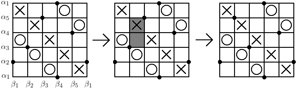
Figure 1. an example of states and a rectangle

There are $n\times n$ squares on $g$ that is separated by $\boldsymbol{\alpha}\cup\boldsymbol{\beta}$. Fix $\mathbf{x,y}\in S$(g), a domain $p$ from $\mathbf{x}$ to $\mathbf{y}$ is a formal sum of the closure of squares satisfying $\partial(\partial_{\alpha}p)=\mathbf{y}-\mathbf{x}$ and $\partial(\partial_{\beta}p)=\mathbf{x}-\mathbf{y}$, where $\partial_{\alpha}p$ is the portion of the boundary of $p$ in the horizontal circles $\alpha_{1}\cup\dots\cup\alpha_{n}$ and $\partial_{\beta}p$ is the portion of the boundary of $p$ in the vertical ones. A domain $p$ is positive if the coefficient of any square is non-negative. Let $\pi(\mathbf{x,y})$ denote the set of domains from $\mathbf{x}$ to $\mathbf{y}$. Throughout the paper, we always assume that a domain is positive. For two domains $p_{1}\in\pi(\mathbf{x,y})$ and $p_{2}\in\pi(\mathbf{y,z})$, the composite domain $p_{1}*p_{2}$ is the domain from $\mathbf{x}$ to $\mathbf{z}$ such that the coefficient of each square is the sum of the coefficient of the square of $p_{1}$ and $p_{2}$. Consider $\mathbf{x,y\in S}(g)$ that coincide with $n-2$ points. An rectangle $r$ from $\mathbf{x}$ to $\mathbf{y}$ is a domain such that $\partial r$ is the union of four segments. A rectangle $r$ is empty if $\mathbf{x}\cap\mathrm{Int}(r)=\mathbf{y}\cap\mathrm{Int}(r)=\emptyset$. Let $\mathrm{Rect}^{\circ}(\mathbf{x,y})$ be the set of empty rectangles from $\mathbf{x}$ to $\mathbf{y}$ if $\mathbf{x}$ and $\mathbf{y}$ coincide with $n-2$ points and $\mathrm{Rect}^{\circ}(\mathbf{x,y})=\emptyset$ otherwise.

Definition 2.1.

The (hat version of) grid chain complex $(\widehat{GC}(g),\widehat{\partial})$ is the $\mathbb{F}$-vector space with basis $\{U_{1}^{k_{1}}\cdots U_{n-1}^{k_{n-1}}\cdot\mathbf{x}|k_{1},\dots,k_{n-1}\geqq 0,\mathbf{x}\in\mathbf{S}(g)\}$, where $\mathbb{F}=\mathbb{Z}/2\mathbb{Z}$ and the $U_{i}$’s are the formal variables corresponding to the $O_{i}$’s in $g$. The differential $\widehat{\partial}$ is the linear map satisfying $U_{i}\circ\widehat{\partial}=\widehat{\partial}\circ U_{i}$ and for $\mathbf{x}\in\mathbf{S}(g)$,

$$\widehat{\partial}(\mathbf{x})=\sum_{\mathbf{y}\in\mathbf{S}(g)}\left(\sum_{\{r\in\mathrm{Rect}^{\circ}(\mathbf{x,y})|r\cap\mathbb{X}=\emptyset,O_{n}\notin r\}}U_{1}^{O_{1}(r)}\cdots U_{n-1}^{O_{n-1}(r)}\right)\mathbf{y},$$

where $O_{i}(r)=1$ if $r$ contains $O_{i}$ and $O_{i}(r)=0$ otherwise for $i=1,\dots,n-1$ and $U_{i}\circ\widehat{\partial}=\widehat{\partial}\circ U_{i}$.

There are two gradings for $\widehat{GC}(g)$, the Maslov grading and the Alexander grading. A planar realization of a toroidal diagram $g$ is a planar figure obtained by cutting toroidal diagram $g$ along $\alpha_{i}$ and $\beta_{j}$ for some $i$ and $j$, and putting on $[0,n)\times[0,n)\in\mathbb{R}^{2}$ in a natural way. For two points $(a_{1},a_{2}),(b_{1},b_{2})\subset\mathbb{R}^{2}$, let $(a_{1},a_{2})<(b_{1},b_{2})$ if $a_{1}<b_{1}$ and $a_{2}<b_{2}$. For two sets of finitely many points $A,B\subset\mathbb{R}^{2}$, let $\mathcal{I}(A,B)$ be the number of pairs $a\in A,b\in B$ with $a<b$ and let $\mathcal{J}(A,B)=(\mathcal{I}(A,B)+\mathcal{I}(B,A))/2$.

Then for $\mathbf{x\in S}(g)$, the Maslov grading $M(\mathbf{x})$ and the Alexander grading $A(\mathbf{x})$ are defined by

(2.1) $$M(\mathbf{x}) =\mathcal{J}(\mathbf{x}-\mathbb{O},\mathbf{x}-\mathbb{O})+1,$$

(2.2) $$A(\mathbf{x}) =\mathcal{J}(\mathbf{x},\mathbb{X}-\mathbb{O})+\frac{1}{2}(\mathcal{J}(\mathbb{O}+\mathbb{X},\mathbb{O}-\mathbb{X}))-\frac{n-1}{2}.$$

These two gradings are extended to the whole $\widehat{GC}(g)$ by

(2.3) $$M(U_{i})=-2,\ A(U_{i})=-1\ (i=1,\dots,n-1).$$

It is known that these two gradings are independent of the choice of the planar realization and that the differential $\widehat{\partial}$ drops the Maslov grading by 1 and preserves or drops the Alexander grading. So $(\widehat{CF}(g),\widehat{\partial})$ is an absolute Maslov graded, Alexander graded chain complex [13, Sections 4.3 and 4.6].

Definition 2.2.

The (hat version of) grid homology of $g$, denoted $\widehat{GH}(g)$, is the homology of $(\widehat{CF}(g),\widehat{\partial})$, thought of as a bigraded vector space.

The grid chain complex $(\widehat{CF}(g),\widehat{\partial})$ depends on which $O$-marking is labeled as $O_{n}$ (Definition 2.1). However, the homology $\widehat{GH}(g)$ up to isomorphism is independent of the choice of $O_{n}$ [13, Corollary 4.6.16]. Moreover, $\widehat{GH}(g)$ is an invariant for knots.

Theorem 2.3 ([13, Theorem 5.3.1]).

Let $g_{1}$ and $g_{2}$ be two grid diagrams representing the same knot $K$. Then $\widehat{GH}(g_{1})\cong\widehat{GH}(g_{2})$ as bigraded vector spaces.

We will denote by $\widehat{GH}(K)$ if there is no confusion.

3. Legendrian and transverse knots with grid diagram

3.1. Legendrian and transverse knots

We briefly review the Legendrian knot and the Legendrian and transverse invariants with grid homology. See [5, 12] for details.

A Legendrian knot is a smooth knot $\mathcal{K}\in\mathbb{R}^{3}$ whose tangent vectors are contained in the contact planes of $\mathrm{Ker}\,\xi_{\mathrm{std}}$, where $\xi_{\mathrm{std}}=dz-y\,dx$. Two knots are Legendrian isotopic if they are connected by a smooth one-parameter family of Legendrian knots. There are two classical invariants of a Legendrian knot $\mathcal{K}$; the Thurston-Bennequin number $\mathrm{tb}(\mathcal{K})$ and the rotation number $\mathrm{r}(\mathcal{K})$. Consider a framing of $\mathcal{K}$ obtained by restricting $\xi_{\mathrm{std}}$ to $\mathcal{K}$ and let $\mathcal{K}^{\prime}$ be the push-off of $\mathcal{K}$ with the framing. Then $\mathrm{tb}(\mathcal{K})$ is defined to be $\ell k(\mathcal{K},\mathcal{K}^{\prime})$. Fix a Seifert surface $F$ for $\mathcal{K}$. The restriction of $\xi_{\mathrm{std}}$ to $F$ gives an oriented two-plane bundle over $F$, which has a trivialization along the $\partial F$ induced by tangent vectors to $\mathcal{K}$. Then $\mathrm{r}(\mathcal{K})$ is the relative Euler number of the two-plane field $\xi_{\mathrm{std}}$ over $F$, relative to the trivialization over $\partial F$. Legendrian knots are studied via their front projections to the $xz$-plane by the projection map $(x,y,z)\mapsto(x,z)$. The front projection of a Legendrian knot has no vertical tangencies and in the generic case, its singularities are double points and cusps. Let $\mathcal{D}$ be the front projection of $\mathcal{K}$. Then we have

$$\mathrm{tb}(\mathcal{K}) =\mathrm{wr}(\mathcal{D})-\frac{1}{2}\#\{\mathrm{cusps\ in}\ \mathcal{D}\},$$

$$\mathrm{r}(\mathcal{K}) =\frac{1}{2}(\#\{\mathrm{downward-oriented\ cusps}\}-\#\{upward-oriented\ cusps\}).$$

Legendrian knots can be locally changed by adding two new cusps, called Legendrian stabilization. Legendrian stabilization preserves the topological knot type, but it changes the Legendrian knot type. Legendrian stabilization drops the Thurston-Bennequin number by one and changes the rotation number by $\pm 1$. The stabilization increasing the rotation number by $1$ is called a positive stabilization and the stabilization drops the rotation number by $1$ is called a negative stabilization.

A transverse knot $\mathcal{T}$ is a knot whose tangent vectors are transverse to the contact planes of $\mathrm{Ker}\,\xi_{\mathrm{std}}$. Two transverse knots are transverse isotopic if they are connected by a smooth one-parameter family of transverse knots. There is a classical invariant for transverse knots $\mathcal{T}$ called self-linking number $\mathrm{sl}(\mathcal{T})$. See [5, Section 2.6.3] for the definition. Given a Legendrian knot $\mathcal{K}$, there are transverse knots $\mathcal{T}$ that are arbitrarily close to $\mathcal{K}$ (in $C^{1}$ topology). Furthermore, there is a neighborhood of $\mathcal{K}$ such that any two transverse knots in this neighborhood are transverse isotopic. The transverse push-off $\mathcal{T}(\mathcal{K})$ of $\mathcal{K}$ is the transverse knot type which can be represented by a transverse knot arbitrarily close to $\mathcal{K}$. Any transverse knot $\mathcal{T}$ is transversely isotopic to the transverse push-off of some Legendrian knot $\mathcal{K}$. Then $\mathcal{K}$ is called Legendrian approximation of $\mathcal{T}$.

3.2. Legendrian knots and grid diagram

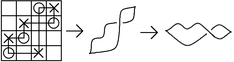
Figure 2. The Legendrian knot determined by a grid diagram

We quickly review the Legendrian knot and the Legendrian and transverse invariants with grid homology. There is an algorithm for giving the front projection of a Legendrian knot from a (planar) grid diagram (Figure 2. See [12, Section 4] and [13, Section 12.2] for details). Let $g$ be a planar grid diagram for a knot $K$. Connect each marking of $g$ by horizontal and vertical segments to obtain a diagram of $K$ on $g$. Rotate $g$ by $45^{\circ}$ clockwise. Turn each corner of the diagram of $K$ on $g$ into cusps or smooth arcs. Switch all crossings of the diagram. Then we get the front projection of the Legendrian knot whose topological type is $m(K)$. We say that a grid diagram $g$ represents the Legendrian knot $\mathcal{K}$ if $\mathcal{K}$ is obtained from $g$ by the above procedure. Furthermore, considering the transverse push-off of $\mathcal{K}$, a grid diagram uniquely specified a transverse knot. Any transverse knot is represented by grid diagrams by taking its Legendrian approximation.

In [12], Ozsváth, Szabó, and Thurston defined Legendrian and transverse invariants using grid homology. For a grid diagram $g$, let $\mathbf{x}^{+}(g)$ be the canonical state consisting of the northeast corner of each square decorated by $X$. Similarly, let $\mathbf{x}^{-}(g)$ be the canonical state consisting of the southwest corner of each square decorated by $X$.

Theorem 3.1 ([12, Theorem 1.1]).

Let $\mathcal{K}$ be a Legendrian knot represented by a grid diagram $g$. The homology classes in $\widehat{GH}(g)$ represented by $\mathbf{x}^{+}(g)$ and $\mathbf{x}^{-}(g)$, denoted by $\widehat{\lambda}_{+}(g)$ and $\widehat{\lambda}_{-}(g)$ respectively, are invariants of Legendrian knots; i.e., if $g$ and $g^{\prime}$ represent Legendrian isotopic knots, then there is a quasi-isomorphism

$$\Phi\colon\widehat{GC}(g)\to\widehat{GC}(g^{\prime})$$

such that $\Phi(\widehat{\lambda}_{+}(g))=\widehat{\lambda}_{+}(g^{\prime})$ and $\Phi(\widehat{\lambda}_{-}(g))=\widehat{\lambda}_{-}(g^{\prime})$.

Theorem 3.2 ([12, Corollary 1.4]).

Let $\mathcal{K}$ be a Legendrian knot represented by a grid diagram $g$, and $\mathcal{T}$ be its transverse push-off. The homology class $\widehat{\lambda}(g)\in\widehat{GH}(g)$, denoted by $\widehat{\theta}(\mathcal{T})$, is an invariant of transverse knot; i.e., if $g$ and $g^{\prime}$ represent two Legendrian approximations to $\mathcal{T}$, then there is a quasi-isomorphism

$$\Psi\colon\widehat{GC}(g)\to\widehat{GC}(g^{\prime})$$

such that $\Psi(\widehat{\theta}(\mathcal{T}))=\widehat{\theta}(\mathcal{T^{\prime}})$.

We remark that the Legendrian invariant $\widehat{\lambda}_{\pm}$ provides obstructions to decomposable Lagrangian cobordisms, certain good cobordisms between two Legendrian knots [1, Theorem 1.2].

4. The preparation of the proof of main theorem

4.1. The construction of grid diagram $g_{\#}$

First, we construct $g_{\#}$ from $g_{1}$ and $g_{2}$.

Definition 4.1.

A grid diagram is called good if it has an $O$-marking in the leftmost square of the top row and in the rightmost square of the bottom row and an $X$-marking in the rightmost square of the top row.

We remark that every knot is represented by a good grid diagram.

Let $g_{\#}$ be the $2n\times 2n$ toroidal diagram so that the four $n\times n$ blocks obtained by cutting it along the horizontal circles $\alpha_{1}\cup\alpha_{n+1}$ and the vertical circles $\beta_{1}\cup\beta_{n+1}$, denoted by $g_{11}$, $g_{12}$, $g_{21}$, and $g_{22}$ respectively (see Figure 3), satisfy the following conditions:

• $g_{11}$ and $g_{1}$ coincide except for the rightmost square of the bottom row.

• $g_{22}$ and $g_{2}$ coincide except for the leftmost square of the top row.

• $g_{12}$ and $g_{21}$ have exactly one $O$-marking.

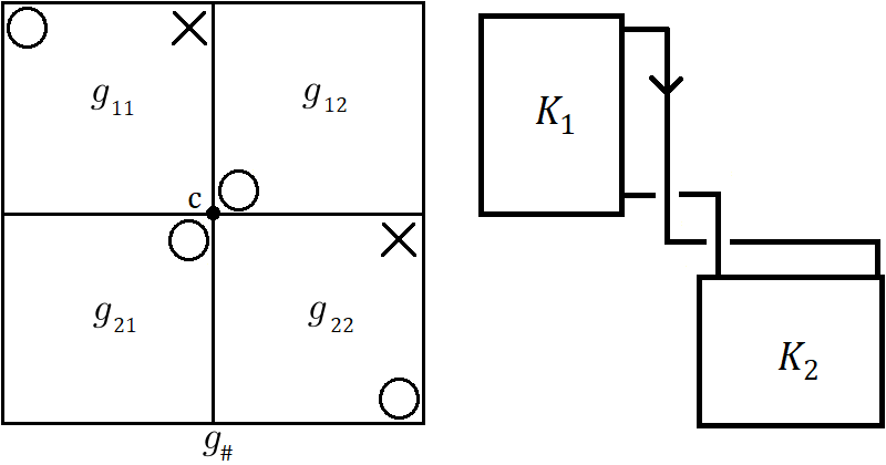
Figure 3. A $2n\times 2n$ grid diagram $g_{\#}$.

Let $O_{i}$ be the $O$-marking in the $i$-th column of $g_{\#}$ $(i=1,\dots,2n)$. Choose $O_{n+1}$ as the special $O$-marking. Then $\widehat{GC}(g)$ is the chain complex of $\mathbb{F}$-vector space with basis $\{U_{1}^{k_{1}}\cdots U_{n}^{k_{n}}\cdot U_{n+2}^{k_{n+2}}\cdots U_{2n}^{k_{2n}}\cdot\mathbf{x}|k_{1},\dots,k_{2n}\geqq 0,\mathbf{x}\in\mathbf{S}(g)\}$.

4.2. The classification of the states $\mathbf{S}(g_{\#})$

The basic idea is the same as [8, Section 5.1]. Let $\mathbf{g}_{11}=(\alpha_{1}\cup\dots\cup\alpha_{n})\cap(\beta_{1}\cup\dots\cup\beta_{n})$ be the $n^{2}$ points in $g_{11}$. Define $\mathbf{g}_{12}$, $\mathbf{g}_{21}$, and $\mathbf{g}_{22}$ similarly. For a state $\mathbf{x}\in\mathbf{S}(g_{\#})$ and $i,j\in\{1,2\}$, let $\mathbf{x}_{ij}=\mathbf{x}\cap\mathbf{g}_{ij}$. We will represent each state $\mathbf{x\in S}(g_{\#})$ uniquely as

$$\mathbf{x}=\begin{pmatrix}\mathbf{x}_{11}&\mathbf{x}_{12}\\ \mathbf{x}_{21}&\mathbf{x}_{22}\\ \end{pmatrix},$$

where $\mathbf{x}_{11}$ and $\mathbf{x}_{22}$ are the $n-k$ points of $\mathbf{x}$ contained in $g_{11}$ and $g_{22}$ respectively, and $\mathbf{x}_{12}$ and $\mathbf{x}_{21}$ is the $k$ points of $\mathbf{x}$ contained in $g_{12}$ and $g_{21}$ respectively.

Take a point $c$ as the intersection point $\alpha_{n+1}\cap\beta_{n+1}$. Let $\mathbf{I}(g_{\#})$ be the set of states that containing $c$ and $\mathbf{N}(g_{\#})=\mathbf{S}(g_{\#})\setminus\mathbf{I}(g_{\#})$. Then, we will classify the states of $\mathbf{I}(g_{\#})$ and $\mathbf{N}(g_{\#})$ as

$$\mathbf{I}_{k}(g_{\#}) =\{\mathbf{x}\in\mathbf{I}(g_{\#})|\#(\mathbf{x}\cap\mathbf{g}_{12})=\#(\mathbf{x}\cap\mathbf{g}_{21})=k\},$$

$$\mathbf{N}_{k}(g_{\#}) =\{\mathbf{x}\in\mathbf{N}(g_{\#})|\#(\mathbf{x}\cap\mathbf{g}_{12})=\#(\mathbf{x}\cap\mathbf{g}_{21})=k\},$$

for $k=0,\dots,n$. Note that since the point $c$ is contained in $\mathbf{g}_{12}$, we have $\mathbf{I}_{0}(g_{\#})=\emptyset$.

5. The proof of the main theorems

5.1. The construction of $f\colon\widehat{GC}(g_{1})\otimes\widehat{GC}(g_{1})\to\widehat{GC}(g_{\#})$

For $i=1,\dots,n$ and $j=1,2$, let $O_{i}^{j}$ be the $O$-marking in the $i$-th column of $g_{j}$. We choose $O_{n}^{1}$ and $O_{1}^{2}$ as the special markings. Then we regard $\widehat{GC}(g_{1})$ as the chain complex of $\mathbb{F}$-vector space with the basis $\{V_{1}^{k_{1}}\cdots V_{n-1}^{k_{n-1}}\cdot\mathbf{x}_{1}|k_{1},\dots,k_{n-1}\geqq 0,\mathbf{x_{1}}\in\mathbf{S}(g_{1})\}$ and $\widehat{GC}(g_{2})$ as the chain complex of $\mathbb{F}$-vector space with the basis $\{W_{2}^{l_{2}}\cdots W_{n}^{l_{n}}\cdot\mathbf{x}_{2}|l_{2},\dots,l_{n}\geqq 0,\mathbf{x_{2}}\in\mathbf{S}(g_{2})\}$, where the indices of the formal variables correspond to the indices of $O$-markings.

For $(\mathbf{x}_{1},\mathbf{x}_{2})\in\mathbf{S}(g_{1})\times\mathbf{S}(g_{2})$, let $\mathbf{x}_{\#}(\mathbf{x}_{1},\mathbf{x}_{2})$ be the state of $\mathbf{N}_{0}(g_{\#})$ naturally obtained by putting $\mathbf{x}_{1}$ and $\mathbf{x}_{2}$ on the $n\times n$ blocks $g_{11}$ and $g_{22}$ respectively.

Definition 5.1.

Let $f\colon\widehat{GC}(g_{1})\otimes\widehat{GC}(g_{2})\to\widehat{GC}(g_{\#})$ be the linear map defined by for $(\mathbf{x}_{1},\mathbf{x}_{2})\in\mathbf{S}(g_{1})\times\mathbf{S}(g_{2})$,

$$f(\mathbf{x}_{1},\mathbf{x}_{2})=\mathbf{x}_{\#}(\mathbf{x}_{1},\mathbf{x}_{2}),$$

and

$$f(V_{i}^{k_{i}})=U_{i}^{k_{i}},\ f(W_{j}^{l_{i}})=U_{n+j}^{l_{i}}.$$

Because $g_{\#}$ is obtained by two good grid diagrams, for a state of $\mathbf{N}_{0}(g_{\#})$, the rectangles counted by the differential of $\widehat{GC}(g_{\#})$ must change either two points in $g_{11}$ or two points in $g_{22}$. In addition, direct computations show that $M(\mathbf{x}_{1})+M(\mathbf{x}_{2})=M(\mathbf{x}_{\#}(\mathbf{x}_{1},\mathbf{x}_{2}))$ and $A(\mathbf{x}_{1})+A(\mathbf{x}_{2})=A(\mathbf{x}_{\#}(\mathbf{x}_{1},\mathbf{x}_{2}))$. Therefore $f$ is a chain map preserving the bigrading.

5.2. Simplification of the chain complex $\widehat{GC}(g_{\#})$

We will observe the tilde-like chain complex of the quotient complex $\widehat{GC}(g_{\#})/\mathrm{Im}f$. In general, there is the simplest version of grid homology called the tilde version which is the chain complex of finite-dimensional vector space. The tilde chain complex is obtained from the hat complex by letting every variable be zero. The homology of the tilde complex and the size of the grid diagram deduce the homology of the hat complex. In order to see that the quotient complex $\widehat{GC}(g_{\#})/\mathrm{Im}f$ is acyclic, we will observe the tilde-like complex of $\widehat{GC}(g_{\#})/\mathrm{Im}f$.

First, we check that multiplication by $U_{i}$ is chain homotopic to multiplication by $U_{n+1}$ if $i\neq n$. Let $X_{i}$ be the $X$-marking of $g_{\#}$ in the $i$-th column of $g_{\#}$ The marking $X_{i}$ is said to be adjacent to $O_{j}$ if these two markings are in the same row or column. For $i\neq n$, let $\widetilde{\mathcal{H}}_{X_{i}}\colon\widehat{GC}(g_{\#})/\mathrm{Im}f\to\widehat{GC}(g_{\#})/\mathrm{Im}f$ be a homotopy operator

$$\widetilde{\mathcal{H}}_{X_{i}}(\mathbf{x})=\sum_{\mathbf{y}\in\mathbf{S}(g_{\#})}\left(\sum_{\{r\in\mathrm{Rect}^{\circ}(\mathbf{x,y})|r\cap\mathbb{X}=\{X_{i}\},O_{n+1}\notin r\}}U_{1}^{O_{1}(r)}\cdots U_{n}^{O_{n}(r)}\cdot U_{n+2}^{O_{n+2}(r)}\cdots U_{2n}^{O_{2n}(r)}\right)\mathbf{y}.$$

This is the induced map of the homotopy operator for the minus chain complex discussed in [13, Lemma 4.6.8].

Lemma 5.2.

Suppose that $X_{i}$ is adjacent to $O_{i}$ and $O_{j}$. If $i,j\neq n$, then

(5.1) $$\widetilde{\partial}\circ\widetilde{\mathcal{H}}_{X_{i}}+\widetilde{\mathcal{H}}_{X_{i}}\circ\widetilde{\partial}=U_{i}-U_{j},$$

assuming that $U_{n+1}=0$.

Proof.

We refer to the notation in [13, Lemmas 4.6.7 and 4.6.9]. For the cases (R-1) and (R-2), the same consequences as in the [13] follow in the same way as [13]. For the case (R-3), we consider the states that give rise to a thin annulus containing $X_{i}$. Let $\mathbf{y}$ be the state that appear in the terms of $\widetilde{\mathcal{H}}_{X_{i}}(\mathbf{x})$. Suppose that there are two rectangles $r_{1}\in\mathrm{Rect}^{\circ}(\mathbf{x,y})$ and $r_{2}\in\mathrm{Rect}^{\circ}(\mathbf{y,x})$ such that $r_{1}*r_{2}$ is the annulus of height or width $1$ and appear in $\widetilde{\partial}\circ\widetilde{\mathcal{H}}_{X_{i}}+\widetilde{\mathcal{H}}_{X_{i}}\circ\widetilde{\partial}$. Because the $X_{i}$ is not in the top row or $n+1$-th row and the annulus $r_{1}*r_{2}$ contains $X_{i}$, both $\mathbf{x,y}$ are either in $\mathbf{N}_{0}(g_{\#})$ or $\mathbf{S}(g_{\#})\setminus\mathbf{N}_{0}(g_{\#})$. Therefore two annuli of height $1$ and width $1$ appear in $\widetilde{\partial}\circ\widetilde{\mathcal{H}}_{X_{i}}+\widetilde{\mathcal{H}}_{X_{i}}\circ\widetilde{\partial}$, so (5.1) holds for $i,j\neq n$. ∎

Proposition 5.3.

Let $C=\frac{\widehat{GC}(g_{\#})/\mathrm{Im}f}{U_{1}=\dots=U_{n-1}=U_{n+2}=\dots=U_{2n}=0}$. Let $W=\mathbb{F}_{0,0}\oplus\mathbb{F}_{-1,-1}$ be the two-dimensional bigraded vector space. Then, there is an isomorphism

$$H(C)\cong H(\widehat{GC}(g_{\#})/\mathrm{Im}f)\otimes W^{\otimes(2n-2)}$$

of bigraded vector spaces.

Proof.

The proof is the same as [13, Proposition 4.6.15]. We remark that by Lemma 5.2, if $i\neq n$, we have $U_{i}\simeq U_{n+1}=0$ in $\widehat{GC}(g_{\#})/\mathrm{Im}f$. ∎

5.3. The proof of Theorem 1.1

proof of Theorem 1.1.

We will see that $\widehat{GC}(g_{\#})/\mathrm{Im}f$ is acyclic. By Proposition 5.3, it is sufficient to prove that $C$ is acyclic.

For $k=1,\dots,n$, let $I_{k}$ and $N_{k}$ be the spans of $\mathbf{I}_{k}(g_{\#})$ and $\mathbf{N}_{k}(g_{\#})$ respectively. Then $\widehat{GC}(g_{\#})$ is a direct sum of infinitely many subspaces, where each summand is written as $U_{1}^{k_{1}}\cdots U_{n}^{k_{n}}\cdot U_{n+2}^{k_{n+2}}\cdots U_{2n}^{k_{2n}}\cdot I_{k}$ or $U_{1}^{k_{1}}\cdots U_{n}^{k_{n}}\cdot U_{n+2}^{k_{n+2}}\cdots U_{2n}^{k_{2n}}\cdot N_{k}$ for non-negative integers $k_{1},\dots,k_{2n}$. By the construction of the chain map $f$ (Section 5.1), as the vector space, $\mathrm{Im}f\cong\bigoplus_{k_{1},\dots,k_{n-1},k_{n+2},\dots,k_{2n}\geqq 0}(U_{1}^{k_{1}}\cdots U_{n-1}^{k_{n-1}}\cdot U_{n+2}^{k_{n+2}}\cdots U_{2n}^{k_{2n}}\cdot N_{0}).$ We remark that $k_{n}=0$ in the above equation. Therefore $C=\frac{\widehat{GC}(g_{\#})/\mathrm{Im}f)}{U_{1}=\dots=U_{n-1}=U_{n+2}=\dots=U_{2n}=0}$ is written as directed sums of infinitely many vector spaces

$$C \cong(N_{1}\oplus\dots\oplus N_{n}\oplus I_{1}\oplus\dots\oplus I_{n})$$

$$\oplus U_{n}\cdot(N_{0}\oplus\dots\oplus N_{n}\oplus I_{1}\oplus\dots\oplus I_{n})$$

$$\oplus U_{n}^{2}\cdot(N_{0}\oplus\dots\oplus N_{n}\oplus I_{1}\oplus\dots\oplus I_{n})$$

$$\oplus\dots$$

Because of the markings on $g_{\#}$, the induced differential $\partial$ of $C$ satisfies that for $j\geqq 1$ and $k\geqq 0$,

$$\partial(U_{n}^{k}N_{j}) \subset U_{n}^{k}N_{j-1}\oplus U_{n}^{k}N_{j}\oplus U_{n}^{k}I_{j}\oplus U_{n}^{k+1}N_{j-1},$$

$$\partial(U_{n}^{k}I_{j}) \subset U_{n}^{k}I_{j-1}\oplus U_{n}^{k}I_{j}\oplus U_{n}^{k+1}N_{j-1},$$

$$\partial(U_{n}^{k}N_{0}) \subset U_{n}^{k}N_{0},$$

where $I_{0}$ is the trivial vector space. We will represent these relations with the following schematic picture:

Then this picture deduces that $U_{n}^{i}I_{1}\oplus U_{n}^{i+1}N_{0}$ forms the subcomplex of $C$ for $i\geqq 0$.

The proof that $C$ is acyclic goes in two steps. First, we will prove that each subcomplex $U_{n}^{i}I_{1}\oplus U_{n}^{i+1}N_{0}$ is acyclic. Then we will check that the quotient complex $C/\bigoplus_{i\geqq 0}(U_{n}^{i}I_{1}\oplus U_{n}^{i+1}N_{0})$ is also acyclic.

1. As each subcomplex $U_{n}^{i}I_{1}\oplus U_{n}^{i+1}N_{0}$ is isomorphic to $I_{1}\oplus U_{n}N_{0}$, it is sufficient to consider $I_{1}\oplus U_{n}N_{0}$. For each state $\mathbf{x}\in\mathbf{I}_{1}(g_{\#})$, the part of $\partial(\mathbf{x})$ into $U_{n}N_{0}$ counts exactly one rectangle. Direct computations show that $\#\mathbf{N}_{0}(g_{\#})=\#\mathbf{I}_{1}(g_{\#})=n!\times n!$. The part of the differential $I_{1}\to U_{n}N_{0}$ is naturally a chain map (Figure 4). Therefore $I_{1}\oplus U_{n}N_{0}$ is acyclic because it forms a mapping cone of an isomorphism.

2. The quotient complex $C/\bigoplus_{i\geqq 0}(U_{n}^{i}I_{1}\oplus U_{n}^{i+1}N_{0})$ is the directed sum of infinitely many copies of $N_{1},\dots,N_{n},I_{2},\dots,I_{n}$ as vector space. Using the following lemma repeatedly, combining [8, Lemmas 5.1 and 5.3], we conclude that the quotient complex $C/\bigoplus_{i\geqq 0}(U_{n}^{i}I_{1}\oplus U_{n}^{i+1}N_{0})$ is acyclic.

Lemma 5.4.

Let $C^{\prime}$ be the subcomplex of $C$. If $C^{\prime}$ and $C/C^{\prime}$ are acyclic, then $C$ is acyclic.

∎

5.4. The proof of Theorem 1.3

Lemma 5.5.

Let $g_{1}$ and $g_{2}$ be good grid diagrams representing Legendrian knots $\mathcal{K}_{1}$ and $\mathcal{K}_{2}$ respectively. Let $g_{\#}$ be the grid diagram from $g_{1}$ and $g_{2}$ (described in Section 4.1). Then $g_{\#}$ represents the connected sum of Legendrian knots $\mathcal{K}_{1}\#\mathcal{K}_{2}$.

Proof.

The front projection determined by $g_{\#}$ naturally represents the connected sum of $K_{1}$ and $K_{2}$, either Legendrian Reidemeister move $1$ (Figure 4).

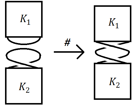
Figure 4. Left$\colon$A front projection of $K_{1}\sqcup K_{2}$. Right$\colon$The front projection determined by $g_{\#}$

∎

proof of Theorem 1.3.

By the construction of $g_{\#}$ and $f$, $f$ sends $\mathbf{x}^{+}(g_{1})\otimes\mathbf{x}^{+}(g_{2})$ to $\mathbf{x}^{+}(g_{\#})$ and $\mathbf{x}^{-}(g_{1})\otimes\mathbf{x}^{-}(g_{2})$ to $\mathbf{x}^{-}(g_{\#})$. Then Lemma 5.5 and Theorem 3.1 complete the proof. ∎

References

- [1] John A. Baldwin, Tye Lidman, and C.-M. Michael Wong, Lagrangian cobordisms and Legendrian invariants in knot Floer homology, Michigan Math. J. 71 (2022), no. 1, 145–175. MR 4389674
- [2] Yuri Chekanov, Differential algebra of Legendrian links, Invent. Math. 150 (2002), no. 3, 441–483. MR 1946550
- [3] Peter R. Cromwell and Ian J. Nutt, Embedding knots and links in an open book. II. Bounds on arc index, Math. Proc. Cambridge Philos. Soc. 119 (1996), no. 2, 309–319. MR 1357047
- [4] Subhankar Dey and Hakan Doğa, A combinatorial description of the knot concordance invariant epsilon, J. Knot Theory Ramifications 30 (2021), no. 6, Paper No. 2150036, 26. MR 4305516
- [5] John B. Etnyre, Legendrian and transversal knots, Handbook of knot theory, Elsevier B. V., Amsterdam, 2005, pp. 105–185. MR 2179261
- [6] Viktória Földvári, The knot invariant using grid homologies, J. Knot Theory Ramifications 30 (2021), no. 7, Paper No. 2150051, 26. MR 4321933
- [7] Hajime Kubota, Concordance invariant for balanced spatial graphs using grid homology, arXiv:2206.15048v2, 2022.
- [8] Hajime Kubota, Grid homology for spatial graphs and a künneth formula of connected sum, 2023.
- [9] Paolo Lisca, Peter Ozsváth, András I. Stipsicz, and Zoltán Szabó, Heegaard Floer invariants of Legendrian knots in contact three-manifolds, J. Eur. Math. Soc. (JEMS) 11 (2009), no. 6, 1307–1363. MR 2557137
- [10] Ciprian Manolescu, Peter Ozsváth, Zoltán Szabó, and Dylan Thurston, On combinatorial link Floer homology, Geom. Topol. 11 (2007), 2339–2412. MR 2372850
- [11] Lenhard Ng, Peter Ozsváth, and Dylan Thurston, Transverse knots distinguished by knot Floer homology, J. Symplectic Geom. 6 (2008), no. 4, 461–490. MR 2471100
- [12] Peter Ozsváth, Zoltán Szabó, and Dylan Thurston, Legendrian knots, transverse knots and combinatorial Floer homology, Geom. Topol. 12 (2008), no. 2, 941–980. MR 2403802
- [13] Peter S. Ozsváth, András I. Stipsicz, and Zoltán Szabó, Grid homology for knots and links, Mathematical Surveys and Monographs, vol. 208, American Mathematical Society, Providence, RI, 2015. MR 3381987
- [14] Sucharit Sarkar, Grid diagrams and the Ozsváth-Szabó tau-invariant, Math. Res. Lett. 18 (2011), no. 6, 1239–1257. MR 2915478
- [15] by same author, Grid diagrams and the Ozsváth-Szabó tau-invariant, Math. Res. Lett. 18 (2011), no. 6, 1239–1257. MR 2915478
- [16] Vera Vértesi, Transversely nonsimple knots, Algebr. Geom. Topol. 8 (2008), no. 3, 1481–1498. MR 2443251