UTBoost: A Tree-boosting based System for Uplift Modeling

Abstract

Uplift modeling refers to the set of machine learning techniques that a manager may use to estimate customer uplift, that is, the net effect of an action on some customer outcome. By identifying the subset of customers for whom a treatment will have the greatest effect, uplift models assist decision-makers in optimizing resource allocations and maximizing overall returns. Accurately estimating customer uplift poses practical challenges, as it requires assessing the difference between two mutually exclusive outcomes for each individual. In this paper, we propose two innovative adaptations of the well-established Gradient Boosting Decision Trees (GBDT) algorithm, which learn the causal effect in a sequential way and overcome the counter-factual nature. Both approaches innovate existing techniques in terms of ensemble learning method and learning objectives, respectively. Experiments on large-scale datasets demonstrate the usefulness of the proposed methods, which often yielding remarkable improvements over base models. To facilitate the application, we develop the UTBoost, an end-to-end tree boosting system specifically designed for uplift modeling. The package is open source and has been optimized for training speed to meet the needs of real industrial applications.

I Introduction

Uplift modeling, a machine learning technique used to estimate the net effect of a particular action, has recently drawn considerable attention. In contrast to traditional supervised learning, uplift models concentrate on modeling the effect of a treatment on individual outcomes and generate uplift scores that show the ”probability of persuasion” for each instance. This technique has proven particularly useful in personalized medicine, performance marketing, and social science. These scenarios are typically presented using tabular data, with each entity having an indicator variable representing whether the subject was treated or not. Additionally, each entity includes a corresponding label.

However, one significant challenge in the uplift problem is the absence of observations for both treated and control responses for an individual in exactly the same context. This hinders the direct application of standard classification techniques to model individual treatment effects. Various tree-based studies [1, 2] have tackled this challenge by creating measures of outcome differences between treated and untreated observations and maximizing heterogeneity between groups. Several researches provide further generalization to bagging ensemble methods on the idea of random forests [3, 4], which aim to address the challenges of tree model performance decay with an increasing number of covariates. Despite the success of these nonparametric methods in prediction, we have experimentally discovered that random-forest based methods still suffer from significant degradation of power in predicting causal effects as the number of variables increases.

An alternative to a random forest is boosted trees. In this paper, we propose an extension to the nonparametric method drawn from a boosting perspective. The subsequent trees are fitted based on the inherited causal effect learned by preceding models. We found that the two ensemble learning methods perform similarly for low-dimensional problems. However, when it comes to modeling extremely high-dimensional data, boosting shows a significant superiority.

However, the split criterion which aim at maximizing heterogeneity neglects the learning of outcomes and focuses solely on uplift signals. This results in limited prediction accuracy and restricts the application of these models in domains where outcome prediction plays a crucial role. In scenarios such as performance marketing, to balance the fairness and profitability of campaigns, the manager selects the objects with respect to both the natural probability of conversion and the predicted incremental score. This prevents customers with a high propensity to purchase from not receiving discounts.

Various studies provide solutions from a potential outcomes estimation standpoint. Among them, meta-learning has gained popularity owing to its ability to utilize any machine learning estimator as base model. Single-Model [9] and Two-Model [10] approaches are two commonly adopted meta learning paradigms. The first model is trained over an entire space, with the treatment indicator serving as an additive input feature. However, this method’s drawback is that a model may not select the treatment indicator if it only uses a subset of features for predictions, such as a tree model. Consequently, the causal effect is estimated as zero for all subjects. An improvement to the Single-Model method is to model the two potential outcomes using two separate models. However, this approach do not utilise the information shared by the control and treated subjects suffer from cumulative errors.

Recently, neural network-based methods becomes the mainstream in uplift modeling. TARNet [14] estimates the causal effect by learning two functions parameterized by two neural networks, utilizing a shared feature representation across treated and control subjects. This method overcomes the limitations of the Two-Models approach through network structural design. However, since TARNet still does not explicitly consider the heterogeneity of causal effects on the loss objective during training, and derives individual causal effects as a by-product of estimating the outcomes. In scenarios with weak causal effects, where the label distributions in different groups are very similar, we find that this method, as well as other approaches that use the potential outcome as the learning objective, show a decline in the performance of predicting individual causality. Beyond this, there are many additional challenges when applying deep models in real-world applications, such as lack of locality, data sparsity (missing values), mixed feature types (numerical and ordinal). This leads to deep learning-based models require more effort from experts to preprocess the data, and making it difficult to achieve consistent performance on various datasets [5].

In this paper, we propose a new nonparametric method called CausalGBM (Causal Gradient Boosting Machine). The proposed method uses the tree model as the base learner and learns both the causal effects and potential outcomes through loss optimization. The method explicitly computes the contribution of causal effects to the loss function at each split selection, avoiding the defect that the treatment indicator may not be picked up in some scenarios where the causal effects are weak. We additionally introduce the second-order gradient information to improve the convergence speed of the model and require fewer data preprocessing steps. Experimental comparisons on four large-scale datasets demonstrate that our model outperforms baseline methods and shows better robustness..

With the widespread use of automated A/B testing platforms in internet scenarios, the dramatically expanding scale of data puts great pressure on model training. In the context of randomized trial, we enhance the computational efficiency of CausalGBM through a multi-objective approximation method. Additional measures, such as histogram-based split finding [6] and sparsity-aware algorithm [7] are incorporated to improve the training speed. We have implemented the proposed algorithms, as well as other widely recognized uplift tree models, in the UTBoost (Uplift Tree Boosting system) software. The system is available as an open source package .

We highlight our contributions as follows:

1. We innovates the uplift tree method that focuses on maximizing heterogeneity by extending the ensemble of trees from bagging to boosting.

2. We fuse potential outcomes and causal effects into the classical GBDT [8] theoretical framework for the first time, and a second-order method is adopted to fit the multi-objective.

3. In the context of randomized trial, we propose a approximate algorithm that reduces the computational complexity of the CausalGBM algorithm.

4. We conduct extensive experiments on large-scale realworld and public datasets. Our models outperform baselines in both effectiveness and training speed on these datasets.

The rest of the paper is organized as follows. In Section 2, we review the existing literature on uplift modeling. Section 3 introduces the causal inference framework and notations. Sections 4 and 5 explain the uplift boosting algorithms. In Section 6, we describe the experiments and report the results. Finally, Section 7 presents our conclusions.

II Related Work

Existing works on uplift modeling can be categorized into different frameworks. One common framework is meta learning [9, 10, 11], which utilizes various machine learning estimators as base learners to estimate treatment effect. Notable examples of meta learning paradigms include Single-Model and Two-Model approaches. The Single-Model method is trained over the entire sample space, combining both treated and control samples, with the treatment indicator as an additional input feature. The Two-Model approach builds two models individually on the treatment and control sample spaces. However, in cases where the population sizes of the two groups are unbalanced, the performance of the corresponding base models may be inconsistent and can negatively impact causal effect estimation performance. To address this issue, the X-learner [12] was proposed, which leverages information learned from the control group to improve the estimation of the treated group and vice versa.

In recent years, representation learning using neural networks has emerged as the mainstream approach for treatment distribution debiasing methods and also applies to uplift modeling. These methods employ networks that consist of both group-dependent layers and shared layers across the treated and control groups. Additionally, they employ various regularization strategies to mitigate treatment bias inherent in the observation data. One such method is the Balancing Neural Network (BNN) [13], which minimizes the discrepancy between the distributions of treatment and control samples using the Integral Probability Metric (IPM). Treatment-Agnostic Representation Network (TARNet) and Counterfactual Regression (CFR) [14] extend the BNN into a two-headed structure in a multi-task learning manner. TARNet and CFR learn two functions based on a shared and balanced feature representation across the treated and control spaces. The similaritypreserved individual treatment effect (SITE) estimation method [15] further improves upon CFR by incorporating additional constraints. It is worth noting that for data from randomized experiments, the distance measure is always equal to zero, in which case each method is similar to the TARNet.

The tree-based method has received significant attention in prior research. [1] put forward decision tree-based methods for uplift modeling that use one of the following splitting criteria: Kullback-Leibler (KL) divergence, squared Euclidean distance (ED), and chi-squared divergence. The authors compare the KL and ED-based models to a few baseline approaches, including the Two Model method, and found that their proposed methods outperform the baselines in the binary-treatment case. [2] proposed the causal tree algorithm through a treatment effect-based splitting criterion. Notably, they introduced the concept of ’honest’ estimation, guaranteeing asymptotic properties of treatment effect estimates.

Furthermore, ensemble methods have seen advancements in improving model performance. [16] presented three uplift AdaBoost algorithms that adaptively adjusted sample weights after each iteration to boost base uplift algorithms. Most ensemble methods use tree-based methods as base learners. [3, 4] proposed uplift ensemble methods inspired by random forests [17]. An alternative to a random forest is boosted trees. This type of methods builds up a function approximation by successively fitting weak learners to the residuals of the model at each step. [18] developed a causal boosting algorithm that employed causal trees as base learners, estimating treatment-specific means rather than treatment effects. The algorithm iteratively updates the residuals for each sample and utilizes them to train the subsequent models. However, updating the residuals on the entire sample set can propagate bias from previous models, and subsequent models may be unable to correct for the transferred bias. We improved the algorithm by restricting the computation of residuals to the samples of the treated group exclusively, which diminishes the association between learners and enables subsequent learners to possess sufficient information for bias correction. Another improved version focuses on optimizing the loss function, which extends the standard gradient boosting algorithm to the realm of causal effect estimation and bridges the gap between the two classes of methods.

III Notation and assumptions

Uplift modeling targets on predicting the incremental change in certain outcomes caused by an intervention for each individual [19, 20]. Suppose that we have access to $n$ independent and identically distributed training examples $\{(\boldsymbol{X}_{i},y_{i},w_{i})\}_{i=1}^{n}$, each of which consists of $p$ features $\boldsymbol{X}_{i}\in\!\mathcal{X}$, an observed outcome $y_{i}\!\in\!\mathbb{R}$, and a binary treatment indicator $w_{i}$ indicating that unit $i$ is under treatment ($w_{i}\!=\!1$) or control ($w_{i}\!=\!0$).

In uplift modeling literature [21], it is typical to assume that the treatment $w_{i}$ is randomly assigned (i.e. $w\perp\boldsymbol{X}$) and we commonly take the following quantity as the learning objective:

$$\tau(\boldsymbol{x})=\mathbb{E}[y_{i}|w_{i}\!=\!1,\boldsymbol{X_{i}}\!=\!\boldsymbol{x}]-\mathbb{E}[y_{i}|w_{i}\!=\!0,\boldsymbol{X_{i}}\!=\!\boldsymbol{x}],$$ (1)

which signifies the uplift on $y$ caused by treatment $w$ for the subjective with feature $\boldsymbol{x}$.

Notice that although we expect to interpret $\tau(x)$ from a causal perspective, (1) is not defined under a causal framework. In the following, we briefly show that under certain assumptions, estimating the uplift $\tau(x)$ is equal to inferring the individual treatment effect, a causal quantity defined in the potential outcomes framework [22, 23]. Let $y_{i}(1)$ and $y_{i}(0)$ be the potential outcomes that would be observed for unit $i$ when $w_{i}=1$ and $0$, respectively. The individual treatment effect (ITE) is defined as

$$\tau_{i}:=y_{i}(1)-y_{i}(0),$$ (2)

and $\mathbb{E}[y_{i}(1)-y_{i}(0)|\boldsymbol{X}_{i}]$ is the best estimator in terms of the mean squared error [12]. In the literature of causal inference [24, 25], it is common to assume the following Assumptions 1-2.

Assumption 1 (consistency)

$y_{i}=y_{i}(1)w_{i}+y_{i}(0)(1-w_{i})$

Assumption 2 (Ignorability)

$\{y_{i}(1),y_{i}(0)\}\perp w_{i}|X_{i}$

Under Assumptions 1-2, we have

$$\mathbb{E}[y(w)|\boldsymbol{X}] \!\stackrel{{\scriptstyle\text{Asp \ref{asp.1}}}}{{=}}\!\mathbb{E}[y(w)|\boldsymbol{X},w]$$

$$\!=\!\mathbb{E}[y(1)w+y(0)(1-w)|\boldsymbol{X},w]\!\stackrel{{\scriptstyle\text{Asp \ref{asp.2}}}}{{=}}\!\mathbb{E}[y|\boldsymbol{X},w],$$

where the 1st and 3rd equation relies on Assumption 1 and 2, respectively, and the 2nd equation can be verified by taking $w\!=\!1,0$. Then we have $\boldsymbol{E}[y(1)-y(0)|\boldsymbol{X}]=\boldsymbol{E}[y|\boldsymbol{X},w=1]-\boldsymbol{E}[y|\boldsymbol{X},w=0]$

To summarize, uplift modeling for $\tau(\boldsymbol{x})$ in (1) is equivalent to estimating the ITE defined in (2) under Assumptions 1-2. Further, if we replace the condition $\{\boldsymbol{X}=\boldsymbol{x}\}$ in (1) to a more rough granularity such as $\{\boldsymbol{X}\in\mathcal{X}_{t}\}$ (e.g., restricting the sample in a leaf node $t$), then the equivalence between Uplift and ITE requires $w$ being randomly assigned, a stronger one than the ignorability Assumption 1. In the following, we focus on the setting with randomly assigned treatment.

IV Tree Boosting for Treatment Effect Estimation

Our first proposed method adopts a sequential learning approach to fit causal effects without focusing on potential outcomes. As the splitting criterion in training process is similar to the standard delta-delta-p (DDP) algorithm [26], which aims to maximize the difference of causal effect between the left and right child nodes, once the boosting method is overlooked. We refer to it as TDDP (Transformed DDP).

IV-A Ensemble Learning via Transformed Label

Taking the decision tree as the base learner, we use a sequence of decision trees to predict the uplift $\tau(\boldsymbol{x})$. As the uplift can not be observed for each sample unit, ensemble method for $\tau(\boldsymbol{x})$ differs from the common supervised-learning scenarios. We explicitly derive the optimizing target for uplift estimation in each iteration of the boosting.

Let $T(\boldsymbol{x};\theta_{j})$ denote a tree model with $\theta_{m}$ denoting its parameters including the way of partitions and estimation within leaf nodes. We aim to predict the uplift via

$$\widehat{\tau}(\boldsymbol{x})=\sum_{j=1}^{M}T(\boldsymbol{x};\theta_{j}).$$ (3)

We learn $T(\boldsymbol{x},\theta_{j})$ sequentially to minimize the loss related to $\widehat{\tau}(\boldsymbol{x})$

Let $u_{m}=\sum_{j=1}^{m}T(\boldsymbol{x},\theta_{j})$ denote the sum of previous $m$ trees. Given $u_{m}$ at the $m$ step, the current loss is ${\mathcal{L}(\tau(x),u_{m}(\boldsymbol{x}))}$, the gradient is

$$\boldsymbol{g}_{m}:=\frac{\partial\mathcal{L}(\tau(\boldsymbol{x}),u_{m}(\boldsymbol{x}))}{\partial{u_{m}}(\boldsymbol{x})}$$

Then $-\boldsymbol{g}_{m}$ suggest a local direction where the loss can be further decreased at the current predictor $u_{m}$. Therefore, in a greedy way, we learn $T(\boldsymbol{x};\theta_{m+1})$ to fit $\boldsymbol{g}_{m}$.

Particularly, in the setting of uplift modeling, the quadratic loss at the $m-$step is

$$\mathcal{L}(\tau(\boldsymbol{x}), u_{m}(\boldsymbol{x}))=$$

$$\frac{1}{2}\Big{\{}\mathbb{E}[y|\boldsymbol{X}=\boldsymbol{x},w=1]-\mathbb{E}[y|\boldsymbol{X}=\boldsymbol{x},w=0]-u_{m}(x)\Big{\}}^{2}$$

where the coefficient $\frac{1}{2}$ is only for the ease of gradient formulation. Then the opposite value of the gradient is

$$- \frac{\partial\mathcal{L}(\tau(\boldsymbol{x}),u_{m}(\boldsymbol{x}))}{\partial u_{m}(\boldsymbol{x})}$$

$$=\mathbb{E}[y|\boldsymbol{X}=\boldsymbol{x},w=1]-\mathbb{E}[y|\boldsymbol{X}=\boldsymbol{x},w=0]-u_{m}(\boldsymbol{x})$$

$$=\mathbb{E}[y-u_{m}(\boldsymbol{x})|\boldsymbol{X}=\boldsymbol{x},w=1]-\mathbb{E}[y|\boldsymbol{X}=\boldsymbol{x},w=0].$$

Therefore, in constructing the $(m\!+\!1)$-th tree $T(\boldsymbol{x};\theta_{m+1})$, we may transform the outcome from the original $y_{i}$ as $y_{i}-u_{m}(\boldsymbol{x})$ for the units with $w_{i}=1$ in the treated group while keep the outcome unchanged for the control group. Then we build the tree based on the transformed outcomes.

To summarize, Algorithm 1 outlines the overall training procedures for TDDP, where the split criterion temporarily serve as placeholders and the details will be introduced in the following subsection IV-B.

Algorithm 1 Gradient Tree Boosting for Uplift Modeling

1:Data: $\mathcal{D}=\left\{(\boldsymbol{X}_{i},y_{i},w_{i})\right\}_{i=1}^{N}$, Shrinkage rate: $\alpha$

2:$u_{M}=\sum_{m=1}^{M}T(\boldsymbol{x};\theta_{m})$

3:Set $u_{0}(\boldsymbol{x})=0$.

4:for $m=1,\cdots,M$ do

5:     Set $y_{i}=y_{i}-T(\boldsymbol{x},\theta_{m-1})$ for $\{i~{}|~{}w_{i}=1\}$.

6:     Build Tree Structure: Recursively Partitions $\mathcal{D}^{m}$:

7:     while the stopping rule is not satisfied do

8:         Select the optimal split $s^{*}$ in the candidate splits by the split criterion.

9:         Split the current node into child nodes by $s^{*}$.

10:     end while

11:     Output the Tree Structure $T_{m}$

12:     Obtain Estimator $T(\boldsymbol{x};\theta_{m})$:

13:     for each leaf node $t_{i}$ of $T_{m}$ do

14:         Get $D^{m}(t_{i})$: the sample units in $D^{m}$ that falls into $t_{i}$.

15:         Estimate Weight: $\widehat{\tau}_{m}(t_{i})=\bar{Y}_{1}(D^{m}(t_{i}))-\bar{Y}_{0}(D^{m}(t_{i}))$.

16:         Output the m-th predictor: $T(x;\theta_{m})=\alpha\widehat{\tau}_{m}(t_{T_{m}}(x))$, where $t_{T_{m}}(x)$ denotes the leaf node that $x$ belongs to in $T_{m}$.

17:     end for

18:end for

IV-B Tree Construction Method

In this subsection, we introduce the split criterion, the core aspect of tree construction..

Split Criterion

Recall that in the conventional CART algorithm [27], the optimal split is selected in a greedy way to minimize the mean squared errors (MSE) at each internal node of the regression tree. However, this is not directly applicable because the unit-level uplift $\tau_{i}$ can not be observed (each unit can only be under treatment or control, rather than both). Only in a group of units, treated and control are both available, and therefore we may compute the aggregation statistics of uplift such as average or variance. Therefore, we need to convert the original unit-level split criterion into a feasible version that relies on the aggregation-level quantity of uplift.

In the next, we will show that minimizing the MSE is equivalent to maximizing the gaps between the average uplift within the split nodes. Consider the split selection at an internal root node $t$ with data $D_{t}:=\{\boldsymbol{X}_{i},y_{i},w_{i}\}_{i=1}^{n_{t}}$. Let $s$ denote a split, $s_{L}$ and $s_{R}$ denote the indices set in the left and right child nodes with sub-sample size $n_{L}$ and $n_{R}$, respectively, under the split ${s}.$ For example, suppose $s=\{x_{j}=a\}$ for a numeric variable $x_{j}$, then $s_{L}=\{i|X_{ij}\leq a\}$ and $s_{R}=\{i|X_{ij}>a\}$. Let $\bar{\tau}_{L}:=\sum_{i\in s_{L}}\frac{\tau_{i}}{n_{L}}$ and $\bar{\tau}_{R}:=\sum_{i\in s_{R}}\frac{\tau_{i}}{n_{R}}$ denote the average uplift in the left and right child nodes, respectively. Then we have the following proposition

Proposition IV.1

Minimizing the mean squared errors of $\tau_{i}$ in the split nodes is equivalent to maximizing the difference between the average uplift within the left and right child nodes, i.e.,

$$\mathop{arg}\!\mathop{min}_{s}\Big{\{}\!\!\sum_{i|i\in s_{L}}\!\!\big{(}\tau_{i}-\bar{\tau}_{L}\big{)}^{2}\!\!+ \sum_{i|i\in s_{R}}\big{(}\tau_{i}-\bar{\tau}_{R}\big{)}^{2}\Big{\}}\!$$

$$\!=\!\mathop{arg}\!\mathop{max}_{s}\big{\{}\frac{n_{L}n_{R}}{n}(\bar{\tau}_{L}-\bar{\tau}_{R})^{2}\big{\}}.$$

Proposition IV.1 guides us to a practical split criterion for the uplift modeling as both $\bar{\tau}_{L}$ and $\bar{\tau}_{R}$ are aggregated values that can be estimated from data. Taking $\bar{\tau}_{L}$ as an example, the definition of $\bar{\tau}_{L}$ involves $\{y_{i}(1),y_{i}(0)\}$ as shown in equation (4),

$$\bar{\tau}_{L}=\frac{\sum_{i\in s_{L}}y_{i}(1)-y_{i}(0)}{n_{L}}=\bar{Y}_{L}(1)-\bar{Y}_{L}(0).$$ (4)

Under randomly assigned treatment, $\bar{Y}(1)$ and $\bar{Y}(0)$ can be estimated by the sample average of $y$ in the treatment and control groups, respectively. Therefore, the optimal split $s^{*}$ is selected by the following rule:

$$s^{*}=\arg\max_{s}\Big{\{}\!\!\frac{n_{L}n_{R}}{n}\big{[}\big{(}\bar{Y}_{L}^{1}-\bar{Y}_{L}^{0}\big{)}-\big{(}\bar{Y}_{R}^{1}-\bar{Y}_{R}^{0}\big{)}\big{]}^{2}\Big{\}},$$ (split criterion)

where $Y_{L}^{1}:=\frac{\sum_{i|i\in s_{L},w_{i}=1}y_{i}}{n_{L}^{1}}$ with $n_{L}^{1}$ denoting the number of treated units in the left child node, and $Y_{L}^{0}$, $Y_{R}^{1}$, $Y_{R}^{0}$ are defined similarly.

Note that TDDP is not strictly a gradient boosting algorithm, because there is no loss function for which we are evaluating the gradient at each step, in order to minimize this loss. Rather, TDDP is an adaptation of gradient boosting on the observed outcomes and encourages weak learners to find treatment effect heterogeneities.

V Causal Gradient Boosting Machine

The TDDP algorithm used to identify the heterogeneity of causal effects skips the fitting of potential outcomes and has limitations in scenarios where potential outcomes are still needed for decision making. Meanwhile, in order to emphasize the importance of causal individual causal effect estimation in the model, we abandon the previous framework of obtaining causal effect estimates derived from outcome prediction. We propose to use CausalGBM (Causal Gradient Boosting Machine) to fit causal effects and outcomes in a single learner. This approach extends the standard gradient boosting algorithm to the field of causal effect estimation, thus bridging the gap between the two classes of methods.

V-A Learning Objective

In order to realize the simultaneous estimation of the two objectives, we split the original single learning task. Under Assumption (1) and Equation (2), we can conduct that:

$$y_{i}=y_{i}(1)w_{i}+y_{i}(0)(1-w_{i})=w_{i}\tau_{i}+y_{i}(0)$$ (5)

This equation reveals that for treated samples, the observed labels are equal to the sum of the potential outcomes and the individual causal effects, whereas for control samples, the observed label are equal to the potential outcomes, and enables us to learn both potential outcomes and individual causal effects indirectly from fitting the observation $y_{i}$.

For a given data set with $n$ samples and $p$ features, we use a tree ensemble model which contains $2M$ additive functions to predict the output:

$$\hat{y_{i}}=\sum_{m=1}^{M}f_{m}(X_{i})+w_{i}\tau_{m}(X_{i}),\ f_{m},\tau_{m}\in\mathcal{F}$$

where $\mathcal{F}=\{f(X)=v_{q(X)},\tau(X)=u_{q(X)}\}(q:\mathbb{R}^{p}\rightarrow T,v\in\mathbb{R}^{T},u\in\mathbb{R}^{T})$ represents the regression trees space. Here $q$ maps each example to the corresponding leaf index in each tree, and $T$ refers to the number of leaves in the tree. Note that leaf weights comprise both $u$ and $v$ in this framework, which is significantly different from the classical regression tree. We will use the decision rules in the trees (given by $q$) to classify instance to leaves and compute the final predictions by summing up the scores by Equation (5) in the corresponding leaves (given by $u,v$). To learn the set of functions that are employed in the ensemble model, we minimize the following objective function:

$$\mathcal{L}(\theta)=\sum_{i}l(y_{i},\hat{y_{i}})$$

Here $l$ is a differentiable convex loss function that measures the difference between the prediction and the observed label. Using the binary decision tree as a meta-learner, we train the ensemble model sequentially to minimize loss. In other words, let $\hat{y_{i}}^{t}$ be the prediction of the i-th instance at the t-th iteration, we add $f_{t}+w_{i}\tau_{t}$ to minimize the following objective:

$$\mathcal{L}^{(t)} =\sum_{i=1}^{n}l(y_{i},\hat{y_{i}}^{(t-1)}+f_{t}(x_{i})+w_{i}\tau_{t}(x_{i}))$$

$$=\sum_{i=1}^{n}l(y_{i},\hat{y_{i}}(0)^{(t-1)}+f_{t}(x_{i})+w_{i}(\hat{\tau_{i}}^{(t-1)}+\tau_{t}(x_{i})))$$

We can conduct the second-order approximation to quickly optimize the objective.

$$\mathcal{L}^{(t)} \simeq\sum_{i=1}^{n}[l(y_{i},\hat{y_{i}}^{(t-1)})+\frac{\partial{l(y_{i},\hat{y}^{(t-1)})}}{\partial\hat{\tau}_{t-1}}\tau_{t}(x_{i})$$

$$+\frac{\partial{l(y_{i},\hat{y}^{(t-1)})}}{\partial\hat{f}_{t-1}}f_{t}(x_{i})+\frac{1}{2}\frac{\partial^{2}{l(y_{i},\hat{y}^{(t-1)})}}{\partial\hat{f}_{t-1}^{2}}f_{t}^{2}(x_{i})$$

$$+\frac{1}{2}\frac{\partial^{2}{l(y_{i},\hat{y}^{(t-1)})}}{\partial\hat{\tau}_{t-1}^{2}}\tau_{t}^{2}(x_{i})+\frac{\partial^{2}{l(y_{i},\hat{y}^{(t-1)})}}{\partial\hat{f}_{t-1}\partial\hat{\tau}_{t-1}}f_{t}(x_{i})\tau_{t}(x_{i})]$$

Under the setting that $w_{i}\in[0,1]$, we can remove the constant terms to obtain the following simplified objective at step $t$:

$$\tilde{\mathcal{L}}^{(t)} =\sum_{i=1}^{n}[w_{i}g_{i}\tau_{t}(x_{i})+\frac{1}{2}w_{i}h_{i}\tau_{t}^{2}(x_{i})+g_{i}f_{t}(x_{i})$$

$$+\frac{1}{2}h_{i}f_{t}^{2}(x_{i})+w_{i}h_{i}\tau_{t}(x_{i})f_{t}(x_{i})]$$

where $g_{i}=\partial_{\hat{y}^{(t-1)}}l(y_{i},\hat{y}^{(t-1)})$ and $h_{i}=\partial_{\hat{y}^{(t-1)}}^{2}l(y_{i},\hat{y}^{(t-1)})$ are first and second order gradient statistics on the loss function. Note that they are defined in the same way as standard gradient trees.

Define $I_{j}=\{i|q(X_{i})=j\}$ as the instance set of leaf $j$, we can rewrite the above equation as:

$$\tilde{\mathcal{L}}^{(t)} =\sum_{j=1}^{T}[(\sum_{i\in I_{j}}w_{i}g_{i}+w_{i}h_{i}f_{j})\tau_{j}+\frac{1}{2}(\sum_{i\in I_{j}}w_{i}h_{i})\tau_{j}^{2}$$

$$+(\sum_{i\in I_{j}}g_{i})f_{j}+\frac{1}{2}(\sum_{i\in I_{j}}h_{i})f_{j}^{2}]$$

We can further derive the optimal values for $f_{j}$ and $\tau_{j}$ of this dual quadratic function and the corresponding optimal weights $v^{*}$ and $u^{*}$. However, it is important to note that solving for both weights simultaneously will result in a significant decrease in the computing efficiency of the algorithm, compared to the standard regression tree, which has a simpler analytic solution for the quadratic function, during training process. This constrains the practical application of the scheme. We will introduce an approximation method to solve this difficulty in the next section.

V-B Multi-objective Approximation

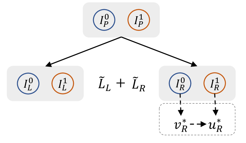
Figure 1: Structure Score Calculation.

We point that if all $w_{i}$ are equal to $0$, i.e., the data set contains only control samples, the above equation is identical to the optimization objective of the regression tree, and we can compute the optimal $v_{0}^{*}$ in that specific context. Under the setting that treatments are assigned randomly, we futher assume that $v^{*}=v_{0}^{*}$ on each leaf, which enables us to derive the optimal weights $v^{*}$ with control instances. After that, the objective function degenerates to a simple quadratic function whith one variable and we can solve optimal $u^{*}$. We can compute the optimal weights by

$$v_{j}^{*} =-\frac{\sum_{i\in I_{j}^{0}}g_{i}}{\sum_{i\in I_{j}^{0}}h_{i}}$$

$$u_{j}^{*} =-\frac{\sum_{i\in I_{j}}w_{i}g_{i}+w_{i}h_{i}v_{j}^{*}}{\sum_{i\in I_{j}}w_{i}h_{i}}=-\frac{\sum_{i\in I_{j}^{1}}g_{i}+h_{i}v_{j}^{*}}{\sum_{i\in I_{j}^{1}}h_{i}}$$

where $I_{j}^{0}=\{i|q(X_{i})=j,w_{i}=0\}$ is the control instance set and $I_{j}^{1}=\{i|q(X_{i})=j,w_{i}=1\}$ is the treated instance set of leaf $j$. It is obvious that, after obtaining $v^{*}$ from the control group, $u^{*}$ is only related to the treated samples. This innovation reduces the original solution process to the sequential solving of two quadratic equations in one variable, which is much simpler, and allows the CausalGBM algorithm is scalable to multiple treatment scenarios with very low additional computational resources, since $u^{*}$ is computed based on the samples of the corresponding group independently of the other groups. The overall computation architecture of CausalGBM is presented in Figure 1. We then calculate the corresponding optimal loss by

$$\tilde{\mathcal{L}}_{global}^{(t)}(q)=\sum_{j=1}^{T}[(\sum_{i\in I_{j}}g_{i})v_{j}^{*}+ \frac{1}{2}(\sum_{i\in I_{j}}h_{i})(v_{j}^{*})^{2}$$

$$-\frac{(\sum_{i\in I_{j}^{1}}g_{i}+h_{i}v_{j}^{*})^{2}}{2\sum_{i\in I_{j}^{1}}h_{i}}]$$

Note that the value is obtained by computing all instances on leaf $I_{j}$ to ensure the global loss is optimized under this approximation method. We provide two other different forms of the optimum value, which are defined as

$$\tilde{\mathcal{L}}_{local}^{(t)}=\sum_{j=1}^{T}[(\sum_{i\in I_{j}^{1}}g_{i})v_{j}^{*}+ \frac{1}{2}(\sum_{i\in I_{j}^{1}}h_{i})(v_{j}^{*})^{2}$$

$$-\frac{(\sum_{i\in I_{j}^{1}}g_{i}+h_{i}v_{j}^{*})^{2}}{2\sum_{i\in I_{j}^{1}}h_{i}}]$$

and

$$\tilde{\mathcal{L}}_{\tau}^{(t)}=\sum_{j=1}^{T}-\frac{(\sum_{i\in I_{j}^{1}}g_{i}+h_{i}v_{j}^{*})^{2}}{2\sum_{i\in I_{j}^{1}}h_{i}}$$

where $I_{j}^{1}=\{i|q(x_{i})=j,w_{i}=1\}$ is the treated instance set of leaf $j$. The first form is only influenced by the treatment group sample, and the other only by the causal effect. We present comparisons of the impact of the different forms for the model in the experimental section.

V-C Greedy Algorithm for Tree Construction

It is impossible to enumerate all tree structures to find the one with the minimum loss value. Instead, we use a greedy algorithm that recursively divides the child nodes starting from a single parent node. Define:

$$\tilde{\mathcal{L}}^{(t)}_{leaf}=(\sum_{i\in I_{leaf}}g_{i})f_{j}^{*}+\frac{1}{2}( \sum_{i\in I_{leaf}}h_{i})(f_{j}^{*})^{2}$$

$$-\frac{(\sum_{i\in I_{leaf}^{1}}g_{i}+h_{i}f_{j}^{*})^{2}}{2\sum_{i\in I_{leaf}^{1}}h_{i}}$$

Assume that $I_{L}$ and $I_{R}$ are the instance sets of left and right nodes after the split. Letting $I=I_{L}\cup I_{R}$, then the loss reduction after the split is given by:

$$\tilde{\mathcal{L}}_{split}=\tilde{\mathcal{L}}^{(t)}_{I}-(\tilde{\mathcal{L}}^{(t)}_{L}+\tilde{\mathcal{L}}^{(t)}_{R})$$

The above function will be used to evaluate the candidate split points. We also incorporate histogram-based split finding [6], sparsity-aware algorithm [7] and other optimizations widely used in regression tree models into UTBoost to improve the efficiency of constructing the tree, which makes the training speed close to the optimal practice and substantially outperforms existing uplift tree softwares.

VI EXPERIMENTS

In order to thoroughly evaluate our proposed methods, we conduct extensive experiments on three large-scale real-world datasets and a synthesized dataset to answer the following research questions:

• Q1: How is the overall performance of TDDP and CausalGBM compared with baseline methods?

• Q2: How does changing the ensemble mode from boosting to bagging influence model performance?

• Q3: Does the performance of the CasualGBM algorithm vary when using different loss computation methods?

• Q4: How well does the CausalGBM perform in terms of outcome prediction?

VI-A Experiment Setup

VI-A1 Datasets

Metrics	CRITEO-UPLIFT1M	HILLSTROM	VOUCHER-UPLIFT	SYNTHETICm
Size	1,000,000	42,693	371,730	200,000
Features	12	8	2076	$m$
Avg. Label	0.047	0.129	0.356	0.600
Treatment Ratio	0.85	0.50	0.85	0.50
Relative Avg. Uplift (%)	26.7	42.6	2.0	50.0

TABLE I: The basic statistics of datasets used in the paper.

We evaluate our proposed models on three large-scale real-world datasets and a synthesized dataset. A summary of these datasets is given in Table I. Here, we briefly introduce them as follows:

• HILLSTROM[28]: A publicly available uplift modeling dataset collected from a randomized experiment of an email advertisement campaign. The dataset contains information about 64,000 customers who last purchased within at most twelve months. The customers were evenly distributed in two treatment groups and a control group, where the first treatment group was sent a ”Men’s Advertisement Email” and the second treatment was sent a ”Women’s Advertisement Email”. The control group received no email. The outcome variables were the visit and conversion status of the customers. We report results on the Women’s merchandise e-mail versus no e-mail split as in previous research.

• CRITEO-UPLIFT[29]: A public dataset consists of 25M rows, with each row representing a user and 11 anonymized features. It also includes a treatment indicator representing whether the customer received a promotional email, as well as two binary labels indicating the visiting and conversion status of the customer. Positive labels mean the user visited/converted on the advertiser’s website during the test period (2 weeks). We randomly selected a subset with 1M instances and used the visit status as the target.

• VOUCHER-UPLIFT: We collect a dataset from a e-commerce platform. 85% of the users were provided with a reminder message with in-account vouchers, with the outcome variable being whether the vouchers was used in the next seven days. The resulting dataset consists of 371,730 samples, each containing 2076-dimensional sparse features, a binary treatment indicator, and a binary label. In order to make the dataset suitable for different algorithms, missing values are filled with zeros.

• SYNTHETIC_m: In order to compare the performances of various methods under ideal data conditions, we adopted the synthesis method proposed by [30]. The dataset contains $m$ variables, a binary indicator and a binary label. About 70% of the variables are associated with both potential outcomes and uplift, and the remaining variables are redundant. The data set consisted of 200K samples, of which 50% were in the treated group and 50% in the control group, and 5% of the samples are randomly labeled.

VI-A2 Baseline Methods

In our experiments, we perform the performance comparison by considering the following three categories of baselines.

Methods Extending Existing Supervised Learning Models. The first category consists of methods that extend existing supervised learning methods for causal effect estimation, which is simple, easy to implement, and has the flexibility of being able to use any off-the-shelf supervised learning algorithm. In this paper, we use LightGBM [6] as the base learner and three variants as baselines:

• The Single-Model Approach[9] . This method uses the concatenation of treatment and covariates $[W,X]$ as the features, and $Y$ as the target to train a supervised model.

• The Two-Model Approach[10]. The two-model approach trains two models on the control and treated subjects separately, and then uses the difference of the two predictions as the estimated conditional average causal effect or uplift.

• Transformed outcome Approach[11]. The transformed outcome approach transforms the observed outcome $Y$ to $Y^{*}$ such that the causal effect equals the conditional expectation of the transformed outcome $Y^{*}$.

• X-Learner[12]. This method includes two models for response estimation, two sub-models for imputed treatment effects estimation, and a propensity model. All models are trained separately without the parameters shared.

Deep Learning-Based Methods. The main advantages of deep learning-based methods are that they can model complex non-linear relationships between the covariates and outcomes, and can handle high-dimensional and large data. In this paper, we select two variants as baselines:

• TARNet[14]. TARNet estimates causal effect by learning two functions parameterised by two neural networks (similar to the two-model approach). Before learning the two functions, TARNet utilises a shared feature representation across the treated and control subjects.

• CFRNet[14]. CFRNet applies an additional loss to the TARNet that forces the learned distributions of the treated and control covariates to be closer to each other. This is measured by either the maximum mean discrepancy (MMD) or the Wasserstein distance.

Tree-Based Methods. Tree-based methods build binary tree models for estimating the treatment effect. We select two ensemble-based approaches as baselines:

• Uplift Random Forest[3]. URF is an uplift ensemble-based method. It consists of two steps. Firstly, it randomly samples a bootstrap training dataset and randomly selects covariates from dataset at each iteration. Secondly, UpliftDT [1] is built on every training dataset from the above step. The set of uplift trees is used to predict the uplift for a new subject by using the average predictions of all trees. We select four splitting criteria based on KL divergence, $\chi^{2}$ divergence, Euclidean and the difference of uplift (DDP) between the two leaves for decision trees.

• Causal Forest[31]. CF is a random forest-like algorithm that directly estimates the treatment effect. This method uses the Causal Tree (CT) algorithm as its base learner, and constructs the forest from an ensemble of $k$ causal trees.

VI-A3 Evaluation Protocols

We perform 10-fold cross-validation and use two widely used metrics in prior work, including area under the ROC curve (AUC) and Qini coefficient [29, 32, 21] (normalized by prefect Qini score) for evaluation, and we perform a grid search on hyperparameters to search for an optimal parameter set that achieved the best performance on the validation dataset, which consisted of 25% of the training dataset in each fold. The parameters we grid-searched included combinations of maximum depth (3, 4, 5) and number of trees (25,50,100,150). Other hyperparameters in algorithms keep their default values. All neural networks of various deep models consist of 128 hidden units with 3 fully connected layers. L2 regularization is applied to mitigate overfitting with a coefficient of 0.01, and the learning rate is set to 0.001 without decay. All deep models are trained with an Adam optimizer with a batch size of 256, and the epoch is determined by the validation set loss. All features input to the neural network are normalized and there are no missing values.

Our experimental environment is a Linux server with a Intel Xeon Platinum 8338C CPU (in total 32 cores) and 128GB memories.

VI-B Overall Performance Comparison (Q1)

Model	HILLSTROM	CRITEO-UPLIFT1M	VOUCHER-UPLIFT	SYNTHETIC100
	Qini Coefficient ($mean\pm s.e.$)
S-LGB	$0.0616\pm 0.0179$	$0.0933\pm 0.0160$	$0.0032\pm 0.0053$	$0.1812\pm 0.0029$
T-LGB	$0.0567\pm 0.0168$	$0.0900\pm 0.0178$	$0.0014\pm 0.0054$	$0.1831\pm 0.0024$
TO-LGB	$0.0377\pm 0.0200$	$0.0941\pm 0.0201$	$0.0048\pm 0.0061$	$0.1832\pm 0.0044$
X-Learner	$0.0619\pm 0.0150$	$0.0929\pm 0.0246$	$0.0029\pm 0.0072$	$0.1824\pm 0.0030$
TARNet	$\underline{0.0636\pm 0.0203}$	$0.0935\pm 0.0109$	$0.0045\pm 0.0076$	$0.1803\pm 0.0049$
CFRNetwass	$0.0635\pm 0.0218$	$0.0909\pm 0.0171$	$0.0042\pm 0.0082$	$0.1829\pm 0.0035$
CFRNetmmd	$0.0629\pm 0.0257$	$0.0923\pm 0.0146$	$0.0047\pm 0.0073$	$0.1808\pm 0.0047$
Causal Forest	$0.0617\pm 0.0139$	$0.0933\pm 0.0113$	$0.0055\pm 0.0041$	$0.1395\pm 0.0039$
URF-Chi	$0.0623\pm 0.0167$	$0.0925\pm 0.0125$	$0.0062\pm 0.0073$	$0.1003\pm 0.0054$
URF-ED	$0.0613\pm 0.0183$	$\underline{0.0942\pm 0.0141}$	$0.0070\pm 0.0064$	$0.1657\pm 0.0057$
URF-KL	$0.0605\pm 0.0160$	$0.0926\pm 0.0123$	$0.0060\pm 0.0055$	$0.1457\pm 0.0036$
URF-DDP	$0.0599\pm 0.0161$	$0.0938\pm 0.0144$	$0.0072\pm 0.0060$	$0.1661\pm 0.0054$
TDDP	$0.0576\pm 0.0123$	$0.0884\pm 0.0179$	$\underline{0.0088\pm 0.0059}$	$\underline{0.1836\pm 0.0045}$
CausalGBM	$\boldsymbol{0.0643\pm 0.0246}$	$\boldsymbol{0.0971\pm 0.0142}$	$\boldsymbol{0.0108\pm 0.0042}$	$\boldsymbol{0.1863\pm 0.0039}$

TABLE II: Model performance evaluated by Qini coefficient on four datasets with corresponding mean and standard error. ”S-”, ”T-”, ”TO-” and ”URF-” stands for instantiations of single-model, two-model, transformed outcome and uplift random forest approaches, respectively. Note that for Qini larger value is better. Best results of all methods are highlighted in boldface.

To verify that our proposed methods can make the uplift prediction model more accurate, we compare TDDP and CausalGBM with different types of baselines and show their prediction performance on four large-scale datasets in Table II. Here, we summarize key observations and insights as follows:

• CausalGBM’s superior performance: Our proposed model CausalGBM outperforms all different baseline methods across all datasets. Specifically, it achieves relative performance gains of 1.1%, 3.1%, 22.7%, and 1.5% on four datasets, respectively, comparing to the best baseline. Further, Qini reflects the model’s ability to give high predicted probabilities of persuasion to those who are actually more likely to be persuaded, and the improvement implies that our proposed model more accurately finds the target population for which the treatment is effective.

• CausalGBM’s robustness across different scenarios: Comparing the results between the four datasets with different scales, we find that many baseline models are not robust in different scenarios. For example, URF-based methods perform significantly better on the HILLSTROM and CRITEO-UPLIFT_1M than on the SYNTHETIC₁₀₀. A plausible reason is that the first two datasets are much smaller than the last two datasets in terms of feature dimensions. As a result the model’s fitting ability is not the key on the first two datasets. In contrast, CausalGBM achieves the best performance in all datasets, which demonstrated our model’s robustness across different scenarios.

  On the VOUCHER-UPLIFT dataset, we observe that deep learning and partial metamodeling-type methods driven by fitting potential outcomes under different treatments are weaker than tree models that focus on the heterogeneity of causal effects. Recall that, as seen in Table I, this dataset has the weakest significance of causal effects of all the datasets. This poses a challenge to methods that focus only on potential outcomes, i.e., the label distributions of the different groups are very similar, which would result in the individual causal effects predicted by this class of methods close to zero. URF-based methods at minimizing heterogeneous differences remain well performing. Since the model of CausalGBM is trained by simultaneously computing both potential outcomes and causal effects, it still performs robustly on the weak causal effect dataset compared to the approaches driven only by potential outcomes.

• An analysis of the volatility for TDDP on different datasets: Comparing TDDP and URF-DDP, the only difference between the two methods lies in the ensemble learning method, the former employs boosting, while the latter takes bagging. Comparing the performances of the two methods on four datasets, TDDP performs better on the dataset with high-dimensional features, while URF-DDP performs better on the dataset consisting of low-dimensional features. A plausible reason is that TDDP overfits the data in datasets with low-dimensional features, meanwhile, URF-DDP does not fit the data in high-dimensional datasets adequately.

VI-C Ablation Study

We compare how the ensemble learning method and the loss form contribute to the predictive performance of the model in this section. In order to better visualize the experimental findings and to prevent the derivation of conclusions from misleading information, we select the synthetic dataset and divide 50% as the training set and the remaining part as the test. Parameters mentioned in the ablation experiments are all self-configurable in the software provided by us, and users can choose their own settings according to the actual characteristics of the dataset.

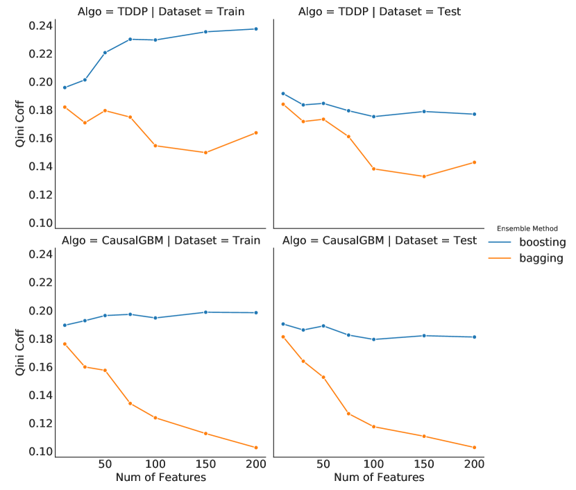
Figure 2: The ablation study on different ensemble methods.

VI-C1 How does ensemble method facilitate the prediction performance? (Q2)

To answer this question, we compare the prediction results of TDDP and CausalGBM with its ablation version, which uses bagging as the ensemble mode. This blocks the updating of the gradient for the CausalGBM algorithm, where the gradient is only computed before the training based on a uniform initial value. The gradient of each sample is constant throughout the training process. Overall, we observe that boosting significantly improves the model’s capability to fit the training data compared to bagging across the two algorithms, and the gap widens as the feature dimensionality grows. Similar conclusions hold for the test dataset. This suggests that boosting provides a significant improvement in model performance, and that this approach is particularly suitable for high-dimensional datasets. On the low-dimensional dataset, the difference between the two methods is relatively small. In addition, we observe that the boosting version of the TDDP method is more likely to overfit the training data with increasing feature size than CausalGBM, leading to a weak generalization performance. In light of this finding, we suggest that tree models that focus on the heterogeneity of local causal effects require regular methods to avoid overfitting compared to the GBM approach that optimizes the global loss function.

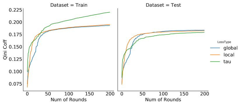
Figure 3: The ablation study on different loss types of CausalGBM.

VI-C2 Which type of loss is appropriate for CausalGBM? (Q3)

We compare the performance of the models under different forms of loss. On the training dataset, $\tilde{\mathcal{L}}_{\tau}$, which focuses only on causal effects, shows superiority in terms of optimization speed and optimal score, significantly outperforming the other two formulations. $\tilde{\mathcal{L}}_{local}$ significantly outperforms $\tilde{\mathcal{L}}_{global}$ in terms of initial improvement optimization speed, and both forms perform similarly in the middle and late stages of training. However, on the test dataset, a contrasting pattern emerges. $\tilde{\mathcal{L}}_{\tau}$ significantly underperforms the other two formulations in the middle stage. After 200 iterations, $\tilde{\mathcal{L}}_{global}$ achieves similarity to $\tilde{\mathcal{L}}_{local}$ in terms of the Qini Coefficient, with both surpassing the performance of $\tilde{\mathcal{L}}_{\tau}$.

We emphasize that if we focus only on the contribution of the causal effect prediction to the loss, the model will not be able to determine whether the prediction of the potential outcome is accurate. Since the causal effects are computed after the potential outcomes are obtained, any bias in the prediction of the outcomes will be transferred to the estimation of the causal effects. This invariably impacts model’s generalization performance. Regarding $\tilde{\mathcal{L}}_{local}$, we highlight that excluding the control group is equivalent to increasing the contribution of the causal effect to the loss, which will force the model to pay more attention to it. There is no significant difference between the two in terms of final predictive performance. However, $\tilde{\mathcal{L}}_{local}$ may outperform $\tilde{\mathcal{L}}_{global}$ in situations where the sample size of the experimental group is much smaller than that of the control group. In such case, the loss value will come predominantly from the control samples. By employing $\tilde{\mathcal{L}}_{local}$, the model effectively mitigates the risk of disregarding causal effects.

VI-D How well does the CausalGBM perform in terms of outcome prediction? (Q4)

Dataset	S-LGB	T-LGB	CausalGBM
	AUC ($mean$)
HILLSTROM	$0.645$	$0.646$	$\boldsymbol{0.648}$
CRITEO-UPLIFT1M	$0.944$	$0.944$	$\boldsymbol{0.946}$
VOUCHER-UPLIFT	$0.850$	$0.851$	$\boldsymbol{0.855}$
SYNTHETIC100	$0.977$	$0.976$	$\boldsymbol{0.979}$

TABLE III: Model performance evaluated by AUC on four datasets.

Two-Models, Single-Model, and CausalGBM are all types of methods that can derive predictions for both potential outcomes and causal effects. Note that we have shown the superiority of CausalGBM over the other two methods on four different datasets with different scales in the ranking of individual causal effects. We will further validate the performance in estimating outcomes and answer why CausalGBM outperforms the other two methods from that perspective.

We take the predicted value of each sample according to its specific group, which is defined as: $\hat{y}_{i}=w_{i}\hat{y}_{i}(1)+(1-w_{i})\hat{y}_{i}(0)$, and use the AUC metric to evaluate the predictive performance on labels. The evaluation results reflect the predictive performance of the model on potential outcomes. We show the experimental results in Table III. CausalGBM slightly outperforms the other two methods on all datasets. We highlight that this improvement is primarily due to differences in the way causal effects are learned, since the models have the same features and both use tree models as learners. Single-Model method treats the indicator variable as a general feature, whereas CausalGBM calculates the gain of this variable at each split. This implies that the latter method will have a higher number of times to fit the causal effect. On the contrary, the Two-Models approach, since the two sub-models are completely independent, implies that the data input to each sub-model is only a part of the full dataset, while a larger amount of data is normally a contributing factor to the model performance.

VI-E Training Speed Comparison

Dataset Size	UTBoost		CausalML
	TDDP	CausalGBM	URF-DDP
$m=30,n=20K$	0.22	0.25	174.4
$m=75,n=20K$	0.47	0.64	499.1
$m=30,n=100K$	0.91	1.10	409.7
$m=75,n=100K$	1.96	2.32	1580.7

TABLE IV: Comparison of training speed (sec) for 50 trees with a maximum depth of 4 on four synthetic datasets.

In addition to model performance, the training efficiency of the model is especially important in real-world application scenarios. We conducted a series of experiments related to efficiency and present the results in Table IV. As can be seen, the training speed of UTBoost is significantly better than that of CausalML [30], which is one of the most popular uplift tree packages. The speedup is primarily brought by the histogram-based approximation algorithm, which speeds up the training by binning the continuous values, and the histogram subtraction method [6] is used for further speedup. UTBoost also incorporates some of the popular URF-based models, and we wish that the improvement in training speed will help the uplift tree model to be widely used and generate more benefits for data engineering.

VII Conclusion

In this paper we formulate two novel boosting methods for the uplift modeling problem. The first algorithm we proposed follows the idea of maximizing the heterogeneity of causal effects. This algorithm differs from the standard regression tree, because there is no loss function for which we are evaluating the gradient at each step, in order to minimize this loss. In contrast, the second algorithm we proposed, CausalGBM, fits both potential outcomes and causal effects by optimizing the loss function. This is similar to standard supervised learning methods. We demonstrate that our proposed techniques outperform the baseline model on large-scale real datasets, where the CausalGBM algorithm shows excellent robustness, while the TDDP algorithm needs to blend in some regularization methods to prevent the model from overfitting the training data. The UTBoost package integrates our proposed new algorithms. The package is open source and out-of-the-box, and achieves state-of-the-art speed in training tree models.

References

- [1] P. Rzepakowski and S. Jaroszewicz, “Decision trees for uplift modeling with single and multiple treatments,” Knowledge and Information Systems, vol. 32, no. 2, pp. 303–327, 2012.
- [2] S. Athey and G. Imbens, “Recursive partitioning for heterogeneous causal effects: Table 1,” Proceedings of the National Academy of Sciences, vol. 113, no. 27, pp. 7353–7360, 2016.
- [3] L. Guelman, M. Guillén, and A. M. Pérez-Marín, “Random forests for uplift modeling: an insurance customer retention case,” in International conference on modeling and simulation in engineering, economics and management. Springer, 2012, pp. 123–133.
- [4] ——, “Uplift random forests,” Cybernetics and Systems, vol. 46, no. 3-4, pp. 230–248, 2015.
- [5] R. Shwartz-Ziv and A. Armon, “Tabular data: Deep learning is not all you need,” Information Fusion, vol. 81, pp. 84–90, 2022.
- [6] G. Ke, Q. Meng, T. Finley, T. Wang, W. Chen, W. Ma, Q. Ye, and T.-Y. Liu, “Lightgbm: A highly efficient gradient boosting decision tree,” Advances in neural information processing systems, vol. 30, 2017.
- [7] T. Chen and C. Guestrin, “Xgboost: A scalable tree boosting system,” ACM, 2016.
- [8] J. H. Friedman, “Greedy function approximation: a gradient boosting machine,” Annals of statistics, pp. 1189–1232, 2001.
- [9] S. Athey and G. W. Imbens, “Machine learning methods for estimating heterogeneous causal effects,” stat, vol. 1050, no. 5, pp. 1–26, 2015.
- [10] N. Radcliffe, “Using control groups to target on predicted lift: Building and assessing uplift model,” Direct Marketing Analytics Journal, pp. 14–21, 2007.
- [11] M. Jaskowski and S. Jaroszewicz, “Uplift modeling for clinical trial data,” in ICML Workshop on Clinical Data Analysis, vol. 46, 2012, pp. 79–95.
- [12] S. R. Künzel, J. S. Sekhon, P. J. Bickel, and B. Yu, “Metalearners for estimating heterogeneous treatment effects using machine learning,” Proceedings of the national academy of sciences, vol. 116, no. 10, pp. 4156–4165, 2019.
- [13] F. Johansson, U. Shalit, and D. Sontag, “Learning representations for counterfactual inference,” in International conference on machine learning. PMLR, 2016, pp. 3020–3029.
- [14] U. Shalit, F. D. Johansson, and D. Sontag, “Estimating individual treatment effect: generalization bounds and algorithms,” in International conference on machine learning. PMLR, 2017, pp. 3076–3085.
- [15] L. Yao, S. Li, Y. Li, M. Huai, J. Gao, and A. Zhang, “Representation learning for treatment effect estimation from observational data,” Advances in neural information processing systems, vol. 31, 2018.
- [16] M. Sołtys and S. Jaroszewicz, “Boosting algorithms for uplift modeling,” arXiv preprint arXiv:1807.07909, 2018.
- [17] L. Breiman, “Random forests.” Machine Learning, vol. 45, 2001.
- [18] S. Powers, J. Qian, K. Jung, A. Schuler, N. H. Shah, T. Hastie, and R. Tibshirani, “Some methods for heterogeneous treatment effect estimation in high dimensions,” Statistics in medicine, vol. 37, no. 11, pp. 1767–1787, 2018.
- [19] R. Gubela, A. Beque, F. Gebert, and S. Lessmann, “Conversion uplift in e-commerce: A systematic benchmark of modeling strategies,” International Journal of Information Technology Decision Making (IJITDM), 2019.
- [20] F. Devriendt, D. Moldovan, and W. Verbeke, “A literature survey and experimental evaluation of the state-of-the-art in uplift modeling: A stepping stone toward the development of prescriptive analytics,” Big Data, vol. 6, no. 1, p. 13, 2018.
- [21] W. Zhang, J. Li, and L. Liu, “A unified survey of treatment effect heterogeneity modelling and uplift modelling,” ACM Computing Surveys (CSUR), 2021.
- [22] J. S. Neyman, “On the application of probability theory to agricultural experiments. essay on principles. section 9.(tlanslated and edited by dm dabrowska and tp speed, statistical science (1990), 5, 465-480),” Annals of Agricultural Sciences, vol. 10, pp. 1–51, 1923.
- [23] D. B. Rubin, “Estimating causal effects of treatments in randomized and nonrandomized studies.” Journal of educational Psychology, vol. 66, no. 5, p. 688, 1974.
- [24] G. W. Imbens and D. B. Rubin, Causal inference in statistics, social, and biomedical sciences. Cambridge University Press, 2015.
- [25] G. W. Imbens and J. M. Wooldridge, “Recent developments in the econometrics of program evaluation,” Journal of economic literature, vol. 47, no. 1, pp. 5–86, 2009.
- [26] B. Hansotia and B. Rukstales, “Incremental value modeling,” Journal of Interactive Marketing, vol. 16, no. 3, pp. 35–46, 2002.
- [27] L. Breiman, J. H. Friedman, R. A. Olshen, and C. J. Stone, Classification and regression trees. Routledge, 2017.
- [28] K. Hillstrom, “The minethatdata e-mail analytics and data mining challenge,” MineThatData blog, 2008.
- [29] E. Diemert, A. Betlei, C. Renaudin, and M.-R. Amini, “A large scale benchmark for uplift modeling,” in KDD, 2018.
- [30] H. Chen, T. Harinen, J.-Y. Lee, M. Yung, and Z. Zhao, “Causalml: Python package for causal machine learning,” 2020.
- [31] S. Wager and S. Athey, “Estimation and inference of heterogeneous treatment effects using random forests,” Journal of the American Statistical Association, vol. 113, no. 523, pp. 1228–1242, 2018.
- [32] P. Gutierrez and J.-Y. Gérardy, “Causal inference and uplift modelling: A review of the literature,” in International conference on predictive applications and APIs. PMLR, 2017, pp. 1–13.