Efficient Enumeration of Recursive Plans in Transformation-based Query Optimizers

Abstract.

Query optimizers built on the transformation-based Volcano/Cascades framework are used in many database systems. Transformations proposed earlier on the logical query dag (LQDAG) data structure, which is key in such a framework, focus only on recursion-free queries. In this paper, we propose the recursive logical query dag (RLQDAG) which extends the LQDAG with the ability to capture and transform recursive queries, leveraging recent developments in recursive relational algebra. Specifically, this extension includes: (i) the ability of capturing and transforming sets of recursive relational terms thanks to (ii) annotated equivalence nodes used for guiding transformations that are more complex in the presence of recursion; and (iii) RLQDAG rewrite rules that transform sets of subterms in a grouped manner, instead of transforming individual terms in a sequential manner; and that (iv) incrementally update the necessary annotations. Core concepts of the RLQDAG are formalized using a syntax and formal semantics with a particular focus on subterm sharing and recursion. The result is a clean generalization of the LQDAG transformation-based approach, enabling more efficient explorations of plan spaces for recursive queries. An implementation of the proposed approach shows significant performance gains compared to the state-of-the-art.

1. Introduction

Recursive queries enable powerful information extraction, especially from linked data structures such as trees and graphs. However, important data management system components, such as the widely used Volcano framework (Graefe and McKenna, 1993), were designed for recursion-free queries. A typical transformation-based query optimizer operates by (i) translating a query into a relational algebraic term, (ii) applying algebraic transformations in order to search for equivalent yet more efficient evaluation plans, during a so-called plan enumeration phase, (iii) executing the query by running one of the explored plans. Works on extending relational algebra (RA) with recursion (Abiteboul et al., 1995; Bancilhon and Ramakrishnan, 1986) resulted in powerful recursive relational algebras (Aho and Ullman, 1979; Agrawal, 1988; Jachiet et al., 2020), capable of capturing queries with transitive closures (Agrawal, 1988) and even more general forms of recursion (Aho and Ullman, 1979; Jachiet et al., 2020). This line of works recently led to $\mu$-RA (Jachiet et al., 2020) which provides a rich set of rewrite rules for recursive terms enabling efficient recursive evaluation plans not available with earlier approaches. The enumeration phase is crucial as it may produce terms which are drastically more efficient. It has been heavily researched for recursion-free queries. It is common practice to allocate a time budget for this enumeration phase, as it is notoriously known that exhaustive plan space explorations may not be feasible in practice for certain queries. The faster we generate the space of equivalent plans, the more likely we will be able to find terms with more efficient evaluation. With recursion, plan spaces are often significantly larger than in the non-recursive setting, due to new interplays between recursive and non-recursive operators. The efficiency of recursive plan enumeration becomes critical. The speed of plan enumeration directly determines whether query evaluation plans enabled by, e.g. $\mu$-RA (Jachiet et al., 2020), are within range or theoretically reachable, but still out of reach for a practical query optimizer. This motivates the search for efficient methods for enumerating recursive plans.

Contributions

We present the recursive logical query dag (RLQDAG), which extends Volcano’s LQDAG (Graefe and McKenna, 1993) and the $\mu$-RA framework (Jachiet et al., 2020) for the purpose of efficiently enumerating recursive query plans. Contributions include the first extension of the LQDAG with the support of recursive terms; a formalization of important RLQDAG concepts in terms of formal syntax and semantics, with a particular focus on the sharing of common subterms in the presence of recursion; RLQDAG transformations that generalize rewrite rules for individual recursive terms of (Jachiet et al., 2020) and enable efficient and grouped transformations of sets of recursive terms. The RLQDAG relies on a concept of annotated equivalence nodes with incremental updates, used for guiding transformations of recursive subterms. Contributions also include a complete implementation of the proposed approach; and experimental assessments using third-party queries on synthetic and real datasets.

2. Background and Related Work

2.1. Approaches in recursive query optimization

Recursion is considered in only a small fraction of the numerous works on query optimization. Three main lines of work with recursive queries can be identified:

• The Datalog line of works (Alvaro et al., 2010; Fan et al., 2019; Francis-Landau et al., 2020; Huang et al., 2011; Seo et al., 2015; Shkapsky et al., 2016; Vianu, 2021; Wang et al., 2015) developed methods for optimizing recursive queries formulated in Datalog: magic-sets  (Bancilhon et al., 1985; Saccà and Zaniolo, 1985; Gardarin, 1987), demand transformations (Tekle and Liu, 2011), automated reversals (Naughton et al., 1989), and the FGH rule (Wang et al., 2022). Although the syntax of Datalog greatly differs from RA, the effects of magic-sets (Bancilhon et al., 1985; Saccà and Zaniolo, 1985; Gardarin, 1987) and of demand transformations (Tekle and Liu, 2011) are comparable to pushing certain kinds of selections and projections. These techniques are very sensitive to whether the Datalog program is written in a left-linear or right-linear manner, but one can use the automated reversal technique proposed in (Naughton et al., 1989) to fully exploit them. The optimization framework proposed in (Wang et al., 2022) gathers magic-sets, semi-naive evaluation and proposes a new FGH rule for optimizing recursive Datalog programs with aggregations.

  Datalog engines do not explore plan spaces but use heuristics to find a good plan to evaluate queries. However, currently, no matter which combination of existing Datalog optimizations a Datalog engine implements, it will not be able to find plans where recursions have been merged automatically similar to those found by the $\mu$-RA approach (Jachiet et al., 2020). This is because, currently, in a Datalog program corresponding to the optimized translation of A⁺/B⁺ at least one of the two transitive closures A⁺ or B⁺ will be fully materialized (even if there is no solution to A⁺/B⁺). On real datasets, this can make Datalog query evaluation an order of magnitude slower than query evaluation with RA-based systems, as noticed in (Jachiet et al., 2020).

• The line of works based on relational algebra (Codd, 1970; Aho and Ullman, 1979; Kifer and Lozinskii, 1990; Agrawal, 1988; Jachiet et al., 2020) attempts to extend relational algebra with operators to capture forms of recursion. For instance, $\alpha$-RA (Agrawal, 1988) extends RA with an operator to capture transitive closures. LFP-RA (Aho and Ullman, 1979) proposes a more general least fixpoint operator, and an extension of this work gave effective criteria for optimization in its presence (Kifer and Lozinskii, 1990). Recently, $\mu$-RA (Jachiet et al., 2020) proposed to extend RA with a $\mu$ operator which is also a fixpoint with an appropriate set of restrictions. This enables $\mu$-RA to combine all earlier RA-based recursion optimization rules in the same framework (Jachiet et al., 2020), while adding new rewrite rules for recursive terms, in particular for merging recursions. This makes $\mu$-RA the most advanced system for RA-based recursive query optimization as it can generate plans not reachable by other approaches. The approach that we propose in this paper extends $\mu$-RA with a new method for enumerating recursive plans much more efficiently, thanks to a generalization of the rules presented in $\mu$-RA so that the generalized rules (presented in Section 4) apply directly on a factorized representation on the recursive plan space. Among the benefits, this makes it possible to apply transformations on sets of algebraic terms at once (instead of successively on individual terms), and to exploit the sharing of common subterms to avoid redundant computations.

• Ad-hoc optimizations for regular queries. Both Datalog-based and RA-based approaches can capture queries with expressive forms of recursion, going beyond regularity. Several works have focused on optimizing queries in which recursion is restricted to regular patterns, such as regular path queries (RPQs). Automata based approaches have been developed to answer RPQ queries (Koschmieder and Leser, 2012; Goldman and Widom, 1997; Zauner et al., 2010). A hybrid approach that combines finite state machines and $\alpha$-RA is presented in (Yakovets et al., 2015) and extended in (Abul-Basher et al., 2017). All these works are limited to RPQs and their unions or conjunctions. In comparison, the work we present in this paper supports more expressive forms of recursion, that may include non-regular patterns (see e.g. the experimental section 5 with queries of the form $A^{n}B^{n}$ for instance).

2.2. Limits of the RA-based approach

The RA line of work offers several advantages including high expressivity and rich plan spaces. In addition, it can be seen as an interesting approach for extending the (non-recursive) RA approach already widely used in RDBMS implementations. One main limit however, is that the whole approach critically depends on the ability to quickly enumerate plans during the plan exploration phase. While plan enumeration has not been studied yet in the presence of recursion, it has been extensively studied for recursion-free queries.

2.3. Plan enumeration for non-recursive (SPJ) queries

Most of the works on plan enumeration focus on select-project-join (SPJ) queries. Techniques proposed for SPJ can be divided into two main groups: bottom-up and top-down approaches. Bottom-up approaches generate the plan space by starting from the leaves (initial relations) and going up in the tree of operators when progressively exploring alternate combinations of operators. In contrast, top-down approaches start from the root and recursively explore subbranches in search for possible alternatives.

2.3.1. Bottom-up approaches

Pioneering and seminal works on the bottom-up approach were proposed in (Selinger et al., 1979) with refinements in execution strategies (Lohman et al., 1985) and the Starburst plan generator (Lohman, 1988; Haas et al., 1989). More recently, E-Graphs (Willsey et al., 2021) and equality saturation techniques (Tate et al., 2011) introduced in the context of SMT solvers have been used in the database community to optimize recursion-free relational and tensor algebra (Wang et al., 2020; Schleich et al., 2023). E-graph (Willsey et al., 2021) basically corresponds to the LQDAG (Graefe and McKenna, 1993) (also known as AND-OR-DAG), as noticed in (Wang et al., 2020). In comparison to LQDAG and E-Graph, that do not support recursive queries, RLQDAG adds the support for recursion. E-Graph is fundamentally bottom-up, whereas RLQDAG relies on top-down search to prune the search space. The top-down aspect of RLQDAG is essential to solve the problem of exploring recursive plans, since transformations of sets of recursive subterms critically rely on a complete view of recursive patterns.

2.3.2. Top-down approaches

The top-down approach was introduced with EXODUS (Graefe and DeWitt, 1987) and the seminal works on Volcano (Graefe and McKenna, 1993) and Cascades (Graefe, 1995) that added memoization to increase efficiency. The purpose of memoization is to re-use information already found in order to avoid redundant calculations. An advantage of the top-down approach is that it makes it possible to use branch and bound pruning, as noticed in (Shapiro et al., 2001).

All the previous approaches focus mainly on SPJ queries, with some extensions to support outer joins (Fender and Moerkotte, 2013a, b; Galindo-Legaria and Rosenthal, 1992, 1997; Moerkotte et al., 2013) and aggregations (Chaudhuri and Shim, 1994). Very few works consider other operators, as noticed in (Chaudhuri, 1998) and (Shanbhag and Sudarshan, 2014). To the best of our knowledge, plan enumeration for transformation-based query optimizers has not been studied yet in the presence of recursive operators.

Union and recursion greatly extend the expressive power of SPJ queries. However, they not only make plan enumeration significantly more complex, but they also generate significantly larger plan spaces. This is because their addition generates many new possible combinations to be explored due to new interplays, for instance between unions and joins (e.g. distributivity of natural join over union) or between recursions and joins. This worsens the combinatorics of plans to be enumerated and motivates even more the interest of finding efficient techniques for enumerating recursive plans.

2.4. The logical query dag (LQDAG)

The method that we propose extends a key component used in the top-down enumeration approach: the logical query dag (LQDAG). The LQDAG is a directed acyclic graph data structure used to represent and generate the logical plan space. It was introduced in (Graefe and McKenna, 1993) and improved in (Graefe, 1995) by the same authors. It is also well described as the AND-OR-DAG in (Roy et al., 2000; Shanbhag and Sudarshan, 2014) where it is used for detecting and unifying common subexpressions for multi-query optimization (Roy et al., 2000); and for generating the space of cross-product free join trees (Shanbhag and Sudarshan, 2014).

The LQDAG contains nodes of two different types: equivalence nodes and operation nodes. Equivalence nodes can only have operation nodes as children and vice versa: operation nodes can only have equivalence nodes as children. The purpose of an equivalence node is to explicitly regroup equivalent subterms. An operation node corresponds to an algebraic operation like: join ($\bowtie$), filter ($\sigma_{\theta}$) etc. The LQDAG can be seen as a factorized representation of a set of terms.

Inspired from (Roy et al., 2000), Figure 1 illustrates a sample LQDAG and its expansion obtained after the application of commutativity and associativity rules for the join operator.

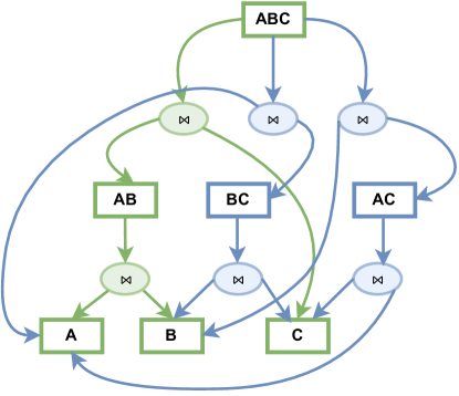
Figure 1. Sample LQDAG (in green) with expansion (in blue).

3. The RLQDAG

The RLQDAG extends the LQDAG with the ability to capture and transform sets of recursive terms.

3.1. Syntax

First of all, we propose a syntax for the RLQDAG. The purpose is to be able to syntactically express a term that denotes a (potentially very large) set of recursive algebraic terms. This makes it possible to develop transformations of sets of terms formally (i.e. with a high level of precision), and express them as rewrite rules that transform one RLQDAG term $d$ into another RLQDAG term $d^{\prime}$. The syntax of RLQDAG terms, given in Fig. 2, focuses on formalizing the concepts of equivalence nodes, operation nodes, sharing of common subterms, and recursion.

$$\begin{array}[]{rcll}{{\gamma}}&\mathrel{::=}&&\!\!\!\!\mbox{Pointer to equivalence node}\\ &&{{\bm{\bigr{[}}\alpha\bm{\bigr{]}}}}&\mbox{Equivalence node}\\ &|&{{\text{ Y }}}&\mbox{Reference}\\ \\ {{\alpha}}&\mathrel{::=}&&\!\!\!\!\mbox{Equivalence node internals}\\ &&{{d}}&\mbox{Operation node}\\ &|&{{d,\alpha}}&\mbox{Operation nodes}\\ &|&{{\text{let Y = $\alpha_{1}$ in $\alpha_{2}$}}}&\mbox{Reference binder}\\ \\ {{d}}&\mathrel{::=}&&\!\!\!\!\mbox{Operation node}\\ &&{X}&\mbox{Relation variable}\\ &|&{\rho_{a}^{b}({{\gamma}})}&\mbox{Rename}\\ &|&{\sigma_{f}({{\gamma}})}&\mbox{Filter}\\ &|&{{\gamma}\bowtie{\gamma^{\prime}}}&\mbox{Join}\\ &|&{{\gamma}\triangleright{\gamma^{\prime}}}&\mbox{Antijoin}\\ &|&{{\gamma}\cup{\gamma^{\prime}}}&\mbox{Union}\\ &|&{\widetilde{\pi}_{a}{({\gamma})}}&\mbox{Antiprojection}\\ &|&{\mu X.\thinspace\gamma\cup\alpha_{rec}}&\mbox{Fixpoint (recursion)}\\ \\ {{\alpha_{rec}}}&\mathrel{::=}&{{\bm{\bigr{[}}\alpha\bm{\bigr{]}}_{\mathfrak{D}}^{\mathfrak{R}}}}&\!\!\!\!\mbox{Annotated equivalence node}\end{array}$$

Figure 2. Syntax of RLQDAG terms.

An equivalence node is a node that can have several operation nodes $d$ as children, possibly with binders. The binder construct “$\text{let}~{}Y~{}=~{}\alpha_{1}~{}\text{in}~{}\alpha_{2}$” enables the explicit sharing of a common equivalence node $\alpha_{1}$ within the branches of another equivalence node $\alpha_{2}$. For that purpose, it assigns a new fresh reference name $Y$ to $\alpha_{1}$, and allows $Y$ to be used multiple times in $\alpha_{2}$ as a reference to $\alpha_{1}$. Hence, the general definition of $\gamma$ is either an equivalence node $\bm{\bigr{[}}\alpha\bm{\bigr{]}}$ or a reference $Y$ to an existing equivalence node.

Operation nodes are defined by the variable $d$ in the abstract syntax of Fig. 2. They include the main algebraic operations of recursive relational algebra. Each operand of an operation node $d$ points in turn to an equivalence node (through $\gamma$). The rename operator $\rho_{\mathsf{a}}^{\mathsf{b}}\left(\gamma\right)$ renames column $a$ into column $b$ in the equivalence node $\gamma$. The filter operator $\sigma_{f}({\gamma})$ applies the filtering expression $f$ to the equivalence node $\gamma$. The antiprojection operator $\widetilde{\pi}_{a}{({\gamma})}$ removes column $a$ from the equivalence node $\gamma$.

For example, with this syntax, the LQDAG of Fig. 1 is written as the term $[[A\bowtie B]\bowtie C]$ before expansion and is written $[[A\bowtie B]\bowtie C,A\bowtie[B\bowtie C],B\bowtie[A\bowtie C]]$ after expansion, where for the sake of readability we omit brackets around relation variables.

Recursive RLQDAGs can be expressed using fixpoint operation nodes. The principle, inspired from earlier works in recursive relational algebras (Aho and Ullman, 1979; Jachiet et al., 2020), consists in the introduction of a least-fixpoint binder operation node ($\mu$) that binds a fresh variable $X$ to some expression in which the variable $X$ can appear, thus explicitly denoting recursion. In the RLQDAG, as defined in the abstract syntax of Fig. 2 and illustrated in Fig. 3, a fixpoint operator node is written $\mu X.~{}\gamma~{}\cup~{}\alpha_{rec}$. The first operand $\gamma$ is an equivalence node that models the constant part (the base case) of the recursion. $X$ cannot occur within $\gamma$. The other equivalence node $\alpha_{rec}$ is the recursive part. An important aspect is that $\alpha_{rec}$ contains at least one free occurrence of the recursive variable $X$. This is a major difference between the fixpoint operation node and the other operation nodes. This aspect will lead to a number of new definitions and formal developments. This is because depending on how the recursive variable is used in that branch, the transformation and sharing of subterms in the RLQDAG may, or may not, be allowed.

For example, on the Yago graph dataset (YAGO, 2019), the query $\mathcal{Q}_{e_{1}}$:

$$\small?s,~{}?t~{}~{}\leftarrow~{}~{}?s~{}~{}\texttt{isLocatedIn+}~{}~{}?t$$

retrieves all pairs ($s,t$) of source and target nodes connected by a path composed of a sequence of edges labeled isLocatedIn (transitive closure). The following RLQDAG term $\Sigma$ corresponds to query $\mathcal{Q}_{e_{1}}$:

$$\small\mu X.~{}\bm{\bigr{[}}\texttt{isLocIn}\bm{\bigr{]}}~{}\cup~{}\bm{\bigr{[}}\widetilde{\pi}_{m}\bm{\bigr{[}}{\rho_{t}^{m}({\bm{\bigr{[}}\texttt{isLocIn}\bm{\bigr{]}}})\bowtie\rho_{s}^{m}({\bm{\bigr{[}}X\bm{\bigr{]}}})}\bm{\bigr{]}}\bm{\bigr{]}}_{\mathfrak{D}}^{\mathfrak{R}}$$

It makes recursion explicit using the fixpoint operator. The equivalence node for the constant part contains the relation variable isLocIn whose column names are $s$ and $t$. The equivalence node for the recursive part is composed of a join between the recursive variable $X$ with the relation variable isLocIn. Here, the path traversal is performed from right to left, by introducing a temporary column name “$m$” and renaming the columns so that the natural join is performed on the only common column “$m$” before “$m$” is discarded by the antiprojection.

Fig. 3 illustrates the RLQDAG of $\mathcal{Q}_{e_{1}}$ with two recursive subterms $\Sigma$ and $\Sigma^{\prime}$. Notice that $\Sigma^{\prime}$ is semantically equivalent to $\Sigma$ and encodes the left to right direction of traversal using a different column renaming in the recursive part.

Figure 3. Structure of recursive terms in RLQDAG.

In a RLQDAG, the recursive equivalence node of each fixpoint operation node is annotated with annotations $\mathfrak{D}$ and $\mathfrak{R}$. These annotations will be useful for guiding the application of transformations and will be defined and explained in Section 3.4.

There are two reasons why we distinguish $\alpha_{rec}$ from a general equivalence node $\alpha$ in the abstract syntax. The first reason is that those equivalence nodes for recursive parts are equipped with annotations (see Section 3.5.). The second reason is that we want to allow a maximum level of sharing while preventing the sharing of subterms with free occurences of a recursive variable. We thus forbid the use of the binding construct to share subterms with free variables.

We consider the following restrictions over the abstract syntax presented in Fig. 2: we consider only positive, linear and non mutually recursive RLQDAG terms: (i) positive means that recursive variables only appear in the left-hand operand of an antijoin operator node; (ii) linear means that one of the operands in a join or antijoin operator node is constant in the free variable; (iii) Non-mutually recursive terms means that fixpoint operator nodes are properly nested so that there is only one free variable in any subbranch of an annotated equivalence node (this variable may occur several times). These restrictions define a subset of RLQDAG terms that simplifies the theory while supporting the encoding of expressive queries like union of conjunctive regular path queries (UCRPQs).

3.2. Semantics of RLQDAG terms

The interpretation of a RLQDAG term is the set of all recursive relational algebraic terms that it represents. Formally, the semantics of a RLQDAG $[\alpha]$ is a set of $\mu$-RA terms as defined by the functions $S_{\alpha}\llbracket\rrbracket$ and $S_{\gamma}\llbracket\rrbracket$ presented in Fig. 4, where $E$ denotes a variable environment used to keep track of the variable definitions introduced by binders for the sharing of subterms. The interpretation of a RLQDAG $[\alpha]$ is $S_{\alpha}\llbracket\alpha\rrbracket_{\emptyset}$.

$\begin{array}[]{rcl}S_{\gamma}\llbracket[\alpha]\rrbracket_{E}&=&S_{\alpha}\llbracket\alpha\rrbracket_{E}\\ S_{\gamma}\llbracket Y\rrbracket_{E}&=&S_{\alpha}\llbracket E(Y)\rrbracket_{E}\vspace{0.3cm}\\ S_{\alpha}\llbracket d\rrbracket_{E}&=&S_{d}\llbracket d\rrbracket\\ S_{\alpha}\llbracket d,\alpha\rrbracket_{E}&=&S_{d}\llbracket d\rrbracket{}\cup S_{\alpha}\llbracket\alpha\rrbracket_{E}\\ S_{\alpha}\llbracket\text{let}~{}Y=\alpha_{1}~{}\text{in}~{}\alpha_{2}\rrbracket_{E}&=&S_{\alpha}\llbracket\alpha_{2}\rrbracket_{E\oplus\{Y\mapsto\alpha_{1}\}}\vspace{0.3cm}{}\\ S_{d}\llbracket X\rrbracket&=&X\\ S_{d}\llbracket\sigma_{f}(\gamma)\rrbracket&=&\{~{}\sigma_{f}(t)\thickspace|\thickspace t\thickspace\in\thickspace S_{\gamma}\llbracket\gamma\rrbracket_{E}\}\\ S_{d}\llbracket\gamma_{1}\bowtie\gamma_{2}\rrbracket&=&\{~{}t\bowtie t^{\prime}~{}\thinspace|\thinspace t\in\thickspace S_{\gamma}\llbracket\gamma_{1}\rrbracket_{E}\land\\ &&~{}\qquad\qquad t^{\prime}\in\thickspace S_{\gamma}\llbracket\gamma_{2}\rrbracket_{E}\}\\ S_{d}\llbracket\gamma_{1}\triangleright\gamma_{2}\rrbracket{}&=&\{~{}t\triangleright t^{\prime}\thinspace|\thinspace t\in\thickspace S_{\gamma}\llbracket\gamma_{1}\rrbracket_{E}\land\\ &&~{}\qquad\qquad t^{\prime}\in\thickspace S_{\gamma}\llbracket\gamma_{2}\rrbracket_{E}\}\\ S_{d}\llbracket\gamma_{1}\cup\gamma_{2}\rrbracket{}&=&\{~{}t\cup t^{\prime}\thinspace|\thinspace t\in\thickspace S_{\gamma}\llbracket\gamma_{1}\rrbracket_{E}\land\\ &&~{}\qquad\qquad t^{\prime}\in\thickspace S_{\gamma}\llbracket\gamma_{2}\rrbracket_{E}\}\\ S_{d}\llbracket\rho_{a}^{b}({\gamma})\rrbracket{}&=&\{~{}\rho_{a}^{b}({t})~{}|\thickspace t\thickspace\in\thickspace S_{\gamma}\llbracket\gamma\rrbracket_{E}\}\\ S_{d}\llbracket\widetilde{\pi}_{a}({\gamma})\rrbracket{}&=&\{~{}\widetilde{\pi}_{a}({t})|\thickspace t\thickspace\in\thickspace S_{\gamma}\llbracket\gamma\rrbracket_{E}\}\\ S_{d}\llbracket\mu X.~{}\gamma~{}\cup~{}\alpha_{rec}\rrbracket{}&=&\{\mu X.~{}t~{}\cup~{}t_{rec}~{}|\thickspace t\thickspace\in\thickspace S_{\gamma}\llbracket\gamma\rrbracket_{E}\\ &&\qquad\qquad\land~{}t_{rec}\thickspace\in\thickspace{S_{\alpha}\llbracket\alpha_{rec}\rrbracket_{E}}\}\end{array}$

Figure 4. Formal semantics of RLQDAG terms, with one interpretation function for each syntactic construct of Fig. 2.

A well-formed RLQDAG is a RLQDAG whose interpretation is a set of semantically equivalent terms:

Definition 1 (Well-formedness).

A RLQDAG $\bm{\bigr{[}}\alpha\bm{\bigr{]}}$ is well-formed if and only if $\forall t,t^{\prime}\in S_{\alpha}\llbracket\alpha\rrbracket_{\emptyset},\quad\texttt{eval}({t})=\texttt{eval}({t^{\prime}})$.

In this definition $\texttt{eval}({t})$ returns the interpretation of the individual recursive relational algebraic term $t$ (i.e. the set of tuples returned by $t$ when evaluated in a database instance).

For example, Fig. 6 illustrates a well-formed RLQDAG capturing two semantically equivalent relational terms obtained before and after the application of join distributivity over union. Fig. 6 illustrates a RLQDAG which is not well-formed, since its top-level equivalence node contains two subterms that are not semantically equivalent.

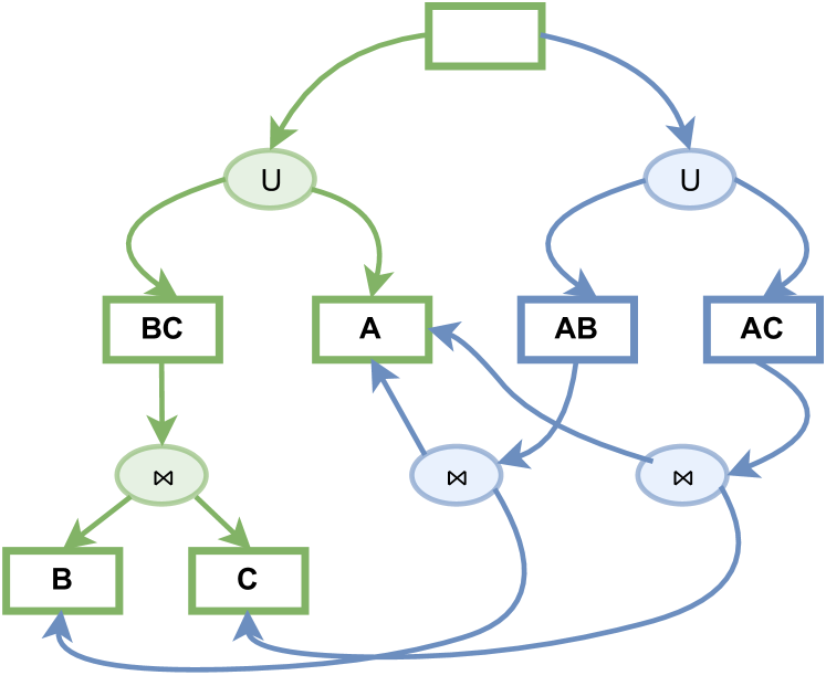
Figure 5. Well-formed RLQDAG.

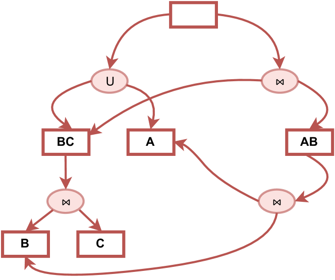
Figure 6. Not well-formed RLQDAG.

The type of an operation node $d$ is the set of column names obtained in the result of the evaluation of any subbranch of $d$. In a well-formed RLQDAG, all $d_{i}$ under the same equivalence node are semantically equivalent, and thus have the same type. For this reason, we also define the type of an equivalence node: $\text{\emph{type}}{(\gamma)}$ as the type of one of its operation nodes. Notice that the type of an annotated equivalence node of some fixpoint operation node $d$ corresponds to the type of the equivalence node of the constant part of $d$. For a given filter operation node $\sigma_{f}({{\gamma}})$, we denote by $\text{\emph{filt(f)}}\subseteq\text{\emph{type}}{(\sigma_{f}({{\gamma}}))}$ the subset of column names used in the filtering function $f$.

3.3. Recursive terms and rule applicability

A significant novelty introduced by recursion when compared to the classical setting of non-recursive algebraic terms resides in the criteria used to trigger rewrite rules. In the classical non-recursive setting these criteria are trivial in the sense that they only depend on top-level operators. In the example of Fig. 6, when applying join distributivity over union, the applicability of the rewrite rule $A\cup(B\bowtie C)~{}\longrightarrow~{}(A\bowtie B)\cup(A\bowtie C)$ can be determined by examining only the combination of the two top-most operators, i.e. the top-level ($\cup$) with the operator immediately underneath (i.e. $\bowtie$).

For some other rewrite rules, applicability criteria may also include some additional verifications such as (non)-interaction between e.g. the set of columns being filtered, or the columns being removed (in the cases of filter and antiprojection, respectively). In the non-recursive setting, these verifications can be done without the need to traverse the whole term. This means that usually no further traversal of subtrees of operators are required. For instance, in the previous example of join distributivity over union, $B$ and $C$ do not need to be traversed at all when determining rule applicability. In sharp contrast, rules for transforming recursive terms rely on criteria that are significantly more sophisticated as they sometimes require a whole traversal of the recursive part of a fixpoint term. This is because opportunities for rule application with recursive terms depend on how the recursive variable is used within the recursive parts of fixpoints. It is known since the works of (Aho and Ullman, 1979; Kifer and Lozinskii, 1990; Jachiet et al., 2020) that criteria for rule application are significantly more sophisticated in the presence of recursion as they need to examine how the recursive variables are used. We show that it is still possible to apply rules over sets of recursive terms at once, using the concept of annotated equivalence nodes, that we define in § 3.5, and for which we need some preliminary definitions.

3.4. Preliminary definitions of auxiliary functions in RLQDAG

Definition 2 (Unfolding).

Let $\alpha$ be an equivalence node. The unfolding of $\alpha$, denoted $\texttt{unfold}(\alpha)$ is $\alpha$ in which all occurrences of equivalence node variable names $Y$ are replaced by their definitions (binders are simply unfolded).

We now define two auxiliary functions over RLQDAG terms. These functions will be used for defining annotated equivalence nodes in Section 3.5.

Notion of destabilizer in RLQDAG

We define the destabilizer of an RLQDAG equivalence node as the set of columns that can be modified by an iteration of a parent fixpoint node. Specifically, destab() traverses subterms and analyzes how the occurrences of free variables are used in order to compute the set of columns that are subject to modifications during a fixpoint node iteration (e.g. renaming or antiprojection).

Definition 3.

For a fixpoint operation node $\mu X.~{}\gamma~{}\cup~{}\alpha_{rec}$ we consider $\alpha^{\prime}=\texttt{unfold}(\alpha_{rec})$ and we define $\texttt{destab}(\alpha^{\prime},X)$ as the following set of column names: $\texttt{destab}(\alpha^{\prime},X)=\{c\in\mathfrak{C}~{}|~{}\exists p\in\texttt{d}(\alpha^{\prime},X)~{}~{}p(c)\neq c\}$ where $\texttt{d}(\cdot,\cdot)$ computes the set of derivations over a RLQDAG term:

$\begin{array}[]{rcl}\texttt{d}((d,\alpha),X)&=&\texttt{d}(d,X)\\ \texttt{d}(\bm{\bigr{[}}\alpha_{1}\bm{\bigr{]}}\cup\bm{\bigr{[}}\alpha_{2}\bm{\bigr{]}},X)&=&\texttt{d}(\alpha_{1},X)\cup\texttt{d}(\alpha_{2},X)\\ \texttt{d}(\bm{\bigr{[}}\alpha_{1}\bm{\bigr{]}}\triangleright\bm{\bigr{[}}\alpha_{2}\bm{\bigr{]}},X)&=&\texttt{d}(\alpha_{1},X)\\ \texttt{d}(\bm{\bigr{[}}\alpha_{1}\bm{\bigr{]}}\bowtie\bm{\bigr{[}}\alpha_{2}\bm{\bigr{]}},X)&=&\texttt{d}(\alpha_{1},X)\cup\texttt{d}(\alpha_{2},X)\\ \texttt{d}(\rho_{a}^{b}({\bm{\bigr{[}}\alpha\bm{\bigr{]}}}),X)&=&\{p\mathbin{\circ}(b\rightarrow a,a\rightarrow\perp)\thickspace|\thickspace p\in\texttt{d}(\alpha,X)\}\\ \texttt{d}(\widetilde{\pi}_{a}{(\bm{\bigr{[}}\alpha\bm{\bigr{]}})},X)&=&\{p\mathbin{\circ}(a\rightarrow\perp)\thickspace|\thickspace p\in\texttt{d}(\alpha,X)\}\\ \texttt{d}(\sigma_{f}(\bm{\bigr{[}}\alpha\bm{\bigr{]}}),X)&=&\texttt{d}(\alpha,X)\\ \texttt{d}(\mu(Z.~{}\gamma~{}\cup~{}\bm{\bigr{[}}\alpha\bm{\bigr{]}}_{\mathfrak{D}}^{\mathfrak{R}}),X)&=&\emptyset\\ \texttt{d}(X,X)&=&\{()\}\thickspace$ (a singleton identity)$\\ \texttt{d}(R,X)&=&\emptyset\\ \end{array}$

and where $\mathbin{\circ}$ represents the composition and $(a_{1}\rightarrow b_{1},...,a_{n}\rightarrow b_{n})$ denotes the function that maps each $a_{i}$ to its $b_{i}$ and every other column name to itself.

For instance, in the RLQDAG of Fig. 3, $\mathfrak{D}=\{s,m\}$ in $\Sigma$ and $\mathfrak{D^{\prime}}=\{t,m\}$ in $\Sigma^{\prime}$. Intuitively, this is because these columns are renamed in front of the recursive variables.

Notion of rigidity in RLQDAG

We define a function rigid() that computes the set of columns that cannot be added nor removed from a fixpoint operation node, without breaking the semantics of the RLQDAG term.

A column $c\in\mathfrak{C}$ cannot be added nor removed from an annotated equivalence node $\alpha_{rec}$ (recursive in $X$) when $c~{}\in~{}\texttt{rigid}(\texttt{unfold}(\alpha),X)$ and rigid() is defined as follows:

Definition 4 (Rigidity).

$\begin{array}[]{rcl}\texttt{rigid}((d,\alpha),X)&=&\texttt{rigid}(d,X)\\ \texttt{rigid}(\bm{\bigr{[}}\alpha_{1}\bm{\bigr{]}}\cup\bm{\bigr{[}}\alpha_{2}\bm{\bigr{]}},X)&=&\texttt{rigid}(\alpha_{1},X)\cup\texttt{rigid}(\alpha_{2},X)\\ \texttt{rigid}(\bm{\bigr{[}}\alpha_{1}\bm{\bigr{]}}\bowtie\bm{\bigr{[}}\alpha_{2}\bm{\bigr{]}},X)&=&\texttt{rigid}(\alpha_{1},X)\cup\texttt{rigid}(\alpha_{2},X)\\ \texttt{rigid}(\bm{\bigr{[}}\alpha_{1}\bm{\bigr{]}}\triangleright\bm{\bigr{[}}\alpha_{2}\bm{\bigr{]}},X)&=&\texttt{rigid}(\alpha_{1},X)\cup\texttt{rigid}(\alpha_{2},X)\\ \texttt{rigid}(\rho_{a}^{b}({\bm{\bigr{[}}\alpha\bm{\bigr{]}}}),X)&=&\texttt{rigid}(\alpha,X)\cup\{a,b\}\\ \texttt{rigid}(\widetilde{\pi}_{a}{(\bm{\bigr{[}}\alpha\bm{\bigr{]}})},X)&=&\emptyset~{}~{}\text{when}~{}X\notin\text{\emph{free}}(\alpha)\\ &=&\texttt{rigid}(\alpha,X)\cup\{a\}~{}\text{otherwise}\\ \texttt{rigid}(\sigma_{f}(\bm{\bigr{[}}\alpha\bm{\bigr{]}}),X)&=&\texttt{rigid}(\alpha,X)\cup\text{\emph{filt}}(f)\\ \texttt{rigid}(\mu(Z.\gamma\cup\bm{\bigr{[}}\alpha\bm{\bigr{]}}_{\mathfrak{D}}^{\mathfrak{R}}),X)&=&\texttt{rigid}(\alpha,X)\cup\texttt{rigid}(\gamma,X)\\ \texttt{rigid}(R,X)&=&type(R)$ when $X\neq R\\ \texttt{rigid}(X,X)&=&\emptyset\\ \end{array}$

For instance, in the RLQDAG of Fig. 3, $\mathfrak{R}=\{s,t\}$ in $\Sigma$. Intuitively, this is because these columns cannot be added nor removed without changing the semantics of the recursion.

3.5. Annotated equivalence node

An annotated equivalence node ($\alpha_{rec}$ in the abstract syntax of RLQDAG terms given in Fig. 2) is an equivalence node of a recursive part of a fixpoint, which is annotated with information that characterize how the recursive variable is used. Specifically:

Definition 5.

Given a RLQDAG operation node $d=\mu X.~{}\gamma~{}\cup~{}\alpha_{rec}$ , the annotated equivalence node $\alpha_{rec}$ is defined as: $\bm{\bigr{[}}\alpha\bm{\bigr{]}}_{\mathfrak{D}}^{\mathfrak{R}}$ where $\mathfrak{D}=\texttt{destab}(\alpha,X)$ and $\mathfrak{R}=\texttt{rigid}(\alpha,X)$.

For example, in the RLQDAG of Fig. 3, the two subterms $\Sigma$ and $\Sigma^{\prime}$ (that correspond to the right-to-left and left-to-right path traversals) carry different annotations: $\mathfrak{D}=\{s,m\}$ in $\Sigma$ whereas $\mathfrak{D^{\prime}}=\{t,m\}$ in $\Sigma^{\prime}$.

Annotations are intended to characterize all the subterms of the annotated equivalence node (thanks to definition 6). The goal of annotated equivalence nodes is to guide and maximize the grouped application of transformations, while also maximizing the sharing of common subterms. In the sequel, we detail RLQDAG transformations, by introducing new rewrite rules capable of transforming sets of subterms at once.

Notion of consistency

Intuitively, a RLQDAG is consistent iff it is well-formed and in addition, for any of its annotated equivalence nodes $\bm{\bigr{[}}\alpha_{2}\bm{\bigr{]}}_{\mathfrak{D}}^{\mathfrak{R}}$, the annotations $\mathfrak{D}$ and $\mathfrak{R}$ are the same for all operation nodes directly underneath (no matter on which subbranch of the equivalence node they are computed, they coincide). More formally:

Definition 6 (Consistency).

A RLQDAG $\bm{\bigr{[}}\alpha\bm{\bigr{]}}$ is consistent iff:

1. it is well-formed;

2. for all fixpoint operator node $\mu X.\thinspace\gamma\cup\bm{\bigr{[}}\alpha_{2}\bm{\bigr{]}}_{\mathfrak{D}}^{\mathfrak{R}}$ occurring in $\alpha$, we have $\texttt{cons}(\alpha_{2},X)_{\mathfrak{D}}^{\mathfrak{R}}$ where: $\begin{array}[]{rcl}\texttt{cons}(\bm{\bigr{[}}d\bm{\bigr{]}},X)_{\mathfrak{D}}^{\mathfrak{R}}&=&\texttt{destab}(d,X)=\mathfrak{D}\\ &&~{}\land~{}\texttt{rigid}(d,X)=\mathfrak{R}\\ \texttt{cons}(\bm{\bigr{[}}d,\alpha\bm{\bigr{]}},X)_{\mathfrak{D}}^{\mathfrak{R}}&=&\texttt{destab}(d,X)=\mathfrak{D}\\ &&~{}\land~{}\texttt{rigid}(d,X)=\mathfrak{R}\\ &&~{}\land~{}\texttt{cons}(\bm{\bigr{[}}\alpha\bm{\bigr{]}},X)_{\mathfrak{D}}^{\mathfrak{R}}\\ \end{array}$

An example of a consistent RLQDAG is shown in Fig. 3 provided $\mathfrak{D},\mathfrak{R},\mathfrak{D^{\prime}}$ and $\mathfrak{R^{\prime}}$ are correctly computed. An example of an inconsistent RLQDAG would be a variant of Fig. 3 with a wrong annotation (e.g. $\mathfrak{D^{\prime}}=\mathfrak{D}$), later exposing the structure to incorrect transformations. This is because incorrect criteria satisfaction might then result in, for example, wrongly pushing a join operation node inside a fixpoint operation node. This would typically produce a not well-formed RLQDAG, breaking the semantics of the initial query. In the remaining, we only consider consistent RLQDAGs.

4. RLQDAG Transformations

We now propose RLQDAG transformations whose purpose is to efficiently build the space of equivalent recursive plans.

RLQDAG transformations capture all the most advanced rewritings of recursive algebraic terms found in previous approaches (e.g. (Agrawal, 1988; Jachiet et al., 2020)). Unlike previous approaches RLQDAG transformations make it possible to systematically group sets of recursive terms and exploit the sharing of common subterms to avoid redundant computations.

RLQDAG transformations leverage annotated equivalence nodes to guide the transformation of recursive subterms. They also update the RLQDAG structure with new annotations when needed, in an incremental manner. The incremental aspect for updating annotations is important as it avoids numerous subterm traversals, thus enabling more efficient grouped transformations.

For each recursive transformation, we describe which subterms can be shared, how newly generated terms are attached and what happens with the other plans already present in the equivalence node. The creation of new combinations of operation nodes may in turn generate more opportunities for transformations that are also explored.

4.1. RLQDAG rewrite rules

We formalize all these ideas by introducing RLQDAG rewrite rules, based on the syntax of RLQDAG terms introduced in Section 3. Specifically, RLQDAG rewrite rules are formalized as functions that take an equivalence node $\gamma$ and return another equivalence node $\gamma^{\prime}$ obtained after applying transformations.

Pushing filters into fixpoint operation nodes

For pushing filters into sets of recursive terms, we introduce a function $\text{pf}()$, defined by considering all the syntactic decomposition cases of the input $\gamma$. Fig. 9 focuses on the two main cases that correspond to potential opportunities of pushing filters, i.e. the cases $\text{pf}(\bm{\bigr{[}}d\bm{\bigr{]}})$ and $\text{pf}(\bm{\bigr{[}}d,\alpha\bm{\bigr{]}})$ where $d$ filters an equivalence node which contains a recursive subterm. For all the other cases, $\text{pf}()$ does not reorder operation nodes in the RLQDAG structure but simply traverses it in search for further transformation opportunities underneath.

$\text{pf}(\bm{\bigr{[}}\sigma_{f}({\bm{\bigr{[}}\mu X.~{}\gamma~{}\cup~{}\bm{\bigr{[}}\alpha\bm{\bigr{]}}_{\mathfrak{D}}^{\mathfrak{R}}\bm{\bigr{]}}})\bm{\bigr{]}})=\newline \mbox{ }~{}\hskip 8.5359pt\left\{\begin{array}[]{ll}\mathbin{\vbox{\hbox{\scalebox{1.1}{$\bullet$}}}}&\bm{\bigr{[}}{\color[rgb]{0,0,1}\mu X^{\prime}.~{}\text{expand}(\bm{\bigr{[}}\sigma_{f}({\gamma})\bm{\bigr{]}})~{}\cup~{}\bm{\bigr{[}}\texttt{expand}({\alpha}_{\{{X}/{X^{\prime}}\}})\bm{\bigr{]}}_{\mathfrak{D}}^{\mathfrak{R^{\prime}}}}~{}~{}\bm{\bigr{]}}\\ &when~{}~{}\text{\emph{filt(f)}}\cap\mathfrak{D}=\emptyset\\ \mathbin{\vbox{\hbox{\scalebox{1.1}{$\bullet$}}}}&\bm{\bigr{[}}~{}~{}\sigma_{f}({\texttt{expand}(\bm{\bigr{[}}\mu X.~{}\gamma~{}\cup~{}\bm{\bigr{[}}\alpha\bm{\bigr{]}}_{\mathfrak{D}}^{\mathfrak{R}}\bm{\bigr{]}})})~{}~{}\bigr{]}~{}~{}{otherwise}\end{array}\right.$

$\text{pf}(\bm{\bigr{[}}\sigma_{f}({\bm{\bigr{[}}\mu X.~{}\gamma~{}\cup~{}\bm{\bigr{[}}\alpha\bm{\bigr{]}}_{\mathfrak{D}}^{\mathfrak{R}},~{}\alpha_{2}\bm{\bigr{]}}})\bm{\bigr{]}})=\newline \mbox{ }~{}\hskip 8.5359pt\left\{\begin{array}[]{ll}\mathbin{\vbox{\hbox{\scalebox{1.1}{$\bullet$}}}}&\bm{\bigr{[}}{\color[rgb]{0,0,1}\mu X^{\prime}.~{}\text{expand}(\bm{\bigr{[}}\sigma_{f}({\gamma})\bm{\bigr{]}})~{}\cup~{}\bm{\bigr{[}}\texttt{expand}({\alpha}_{\{{X}/{X^{\prime}}\}})\bm{\bigr{]}}_{\mathfrak{D}}^{\mathfrak{R^{\prime}}}},\\ &\quad\texttt{expand}(\bm{\bigr{[}}\sigma_{f}({\bm{\bigr{[}}\alpha_{2}\bm{\bigr{]}}})\bm{\bigr{]}})~{}~{}\bm{\bigr{]}}\\ &{when}~{}~{}\text{\emph{filt(f)}}\cap\mathfrak{D}=\emptyset\\ \mathbin{\vbox{\hbox{\scalebox{1.1}{$\bullet$}}}}&\bm{\bigr{[}}~{}~{}\sigma_{f}({\texttt{expand}(\bm{\bigr{[}}\mu X.~{}\gamma~{}\cup~{}\bm{\bigr{[}}\alpha\bm{\bigr{]}}_{\mathfrak{D}}^{\mathfrak{R}},~{}\alpha_{2}\bm{\bigr{]}})})~{},\\ &\quad\texttt{expand}(\bm{\bigr{[}}\sigma_{f}({\bm{\bigr{[}}\alpha_{2}\bm{\bigr{]}}})\bm{\bigr{]}})~{}~{}\bigr{]}~{}~{}{otherwise}\end{array}\right.$

where $\mathfrak{R^{\prime}}=\mathfrak{R}\cup\text{\emph{filt(f)}}$ and ${\alpha}_{\{{X}/{X^{\prime}}\}}$ denotes $\alpha$ in which all occurrences of $X$ are replaced by $X^{\prime}$.

Figure 7. Pushing a filter in an equivalence node containing a fixpoint.

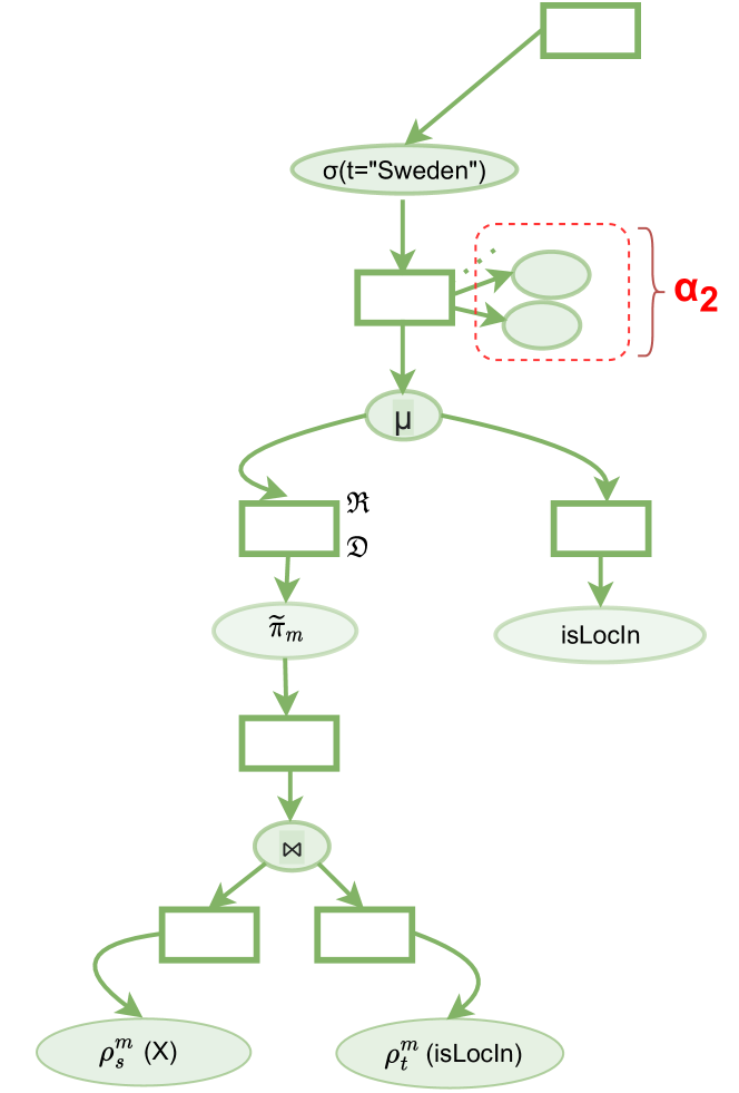
Figure 8. Initial RLQDAG before expansion with opportunity to apply pf().

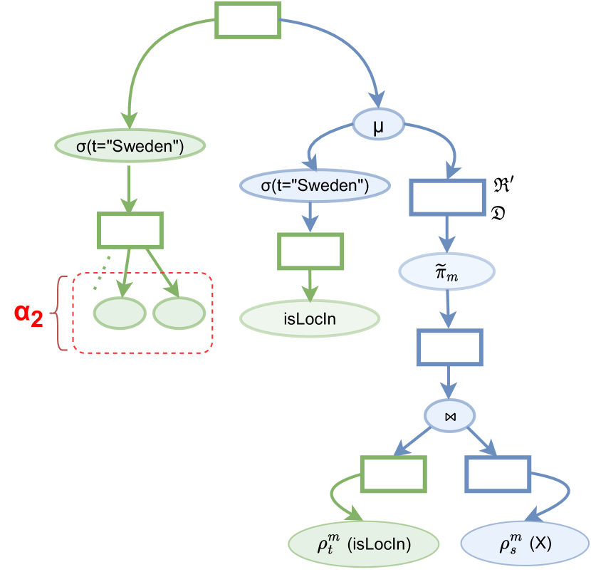
Figure 9. Expansion of a RLQDAG by pushing a filter in a fixpoint operation node, with branches added by $\text{pf}()$ in blue color.

In Fig. 9, whenever the filter can be pushed through the fixpoint operation node, $\text{pf}()$ generates a new RLQDAG in which the filter operation node is put within the constant part of the fixpoint operation node. In the resulting equivalence node, the initial (suboptimal) term is replaced by the new term where filtering is done earlier (hence more efficient). For this transformation to happen, the criteria (on the last line of Fig. 9) must be satisfied. Whenever it is not the case, the RLQDAG structure is not reordered but simply recursively traversed in search for more transformation opportunites. The creation of new combinations of operation nodes may in turn provide new opportunities for other rewritings (for instance, new opportunities for pushing filters even further, or even other kinds of rewritings). This is the role of the $\texttt{expand}()$ function, formally defined in section  4.2. Intuitively, a call to $\texttt{expand}()$ on an equivalence node may further populate the equivalence node with new subterms. The $\texttt{expand}()$ function is in charge of exploring all opportunities for transformations. This is useful because other rewrite rules may apply, and the $\texttt{expand}()$ function basically triggers all possible applications of all rewrite rules.

For example, the query $\mathcal{Q}_{e_{2}}$:

$\footnotesize?s~{}~{}\leftarrow~{}~{}?s~{}~{}\texttt{isLocatedIn+}~{}~{}\text{Sweden}$

retrieves all nodes that are connected to the constant node “Sweden” by a path composed of a sequence of edges labeled isLocatedIn from the Yago graph dataset (YAGO, 2019). Fig. 9 illustrates graphically a portion of $\mathcal{Q}_{e_{2}}$ RLQDAG, and Fig. 9 depicts its updated structure obtained after the pushing filter transformation defined in Fig. 9. New branches created by $\text{pf}()$ are represented in blue color. The new term is added in the same equivalence node as the previous term, since they are semantically equivalent. Notice the incremental update of annotations performed by $\text{pf}()$ in Fig. 9: the annotations of the newly created term (in blue) are obtained from the annotations of the initial term. In that case $\mathfrak{D}$ is simply propagated whereas $\mathfrak{R^{\prime}}=\mathfrak{R\cup\text{\emph{filt(f)}}}$.

Pushing joins into fixpoint operation nodes

For pushing joins into sets of recursive terms we define a function $\text{pj}()$. $\text{pj}()$ takes an equivalence node $\gamma$ as input and returns an expanded equivalence node $\gamma^{\prime}$ that contains all the subterms in $\gamma$ with, in addition, all the subterms where all joins pushable in fixpoint operation nodes have been pushed. We define $\text{pj}()$ for all possible syntactic decompositions of a RLQDAG. Fig. 11 presents the definition of $\text{pj}($) for the two main cases of interest. Again, other cases are defined without structure rearrangement but involving recursive calls to $\texttt{expand}()$ in search for further transformation opportunites underneath. Notice that whenever a join can be pushed within a fixpoint operation node (see Fig. 11), it is possible to share the constant part of the fixpoint operation node. This is made explicit by the creation of the outermost “let” binder whose goal is to define and associate a name to the equivalence node, so that it can be referred multiple times (thus explicitly showing the sharing of subterms).

For example, the query $\mathcal{Q}_{e_{3}}$:

$\footnotesize?s,~{}?t~{}~{}\leftarrow~{}~{}?s~{}~{}\texttt{haschild+/livesin}~{}~{}?t$

retrieves all pairs of nodes that are connected by a path composed of a sequence of edges labeled haschild followed by a single edge labeled livesin. Fig. 11 illustrates graphically a portion of $\mathcal{Q}_{e_{3}}$ RLQDAG, after the application of the rule that pushes joins into fixpoint operation nodes described in Fig. 11. Fig. 11 shows that the newly created branch (in blue color) extends the set of semantically equivalent terms of the existing equivalence node.

$\text{pj}(\bm{\bigr{[}}\beta\bowtie{\bm{\bigr{[}}\mu X.~{}\gamma~{}\cup~{}\bm{\bigr{[}}\alpha\bm{\bigr{]}}_{\mathfrak{D}}^{\mathfrak{R}}\bm{\bigr{]}}}\bm{\bigr{]}})=\newline \mbox{ }~{}\hskip 8.5359pt\left\{\begin{array}[]{ll}\mathbin{\vbox{\hbox{\scalebox{1.1}{$\bullet$}}}}&\text{let const}=\gamma~{}\text{in}{}\\ &\quad\bm{\bigr{[}}~{}~{}\bm{\bigr{[}}\texttt{expand}(\beta)\bowtie\texttt{expand}(\bm{\bigr{[}}\mu X.~{}\text{const}~{}\cup~{}\bm{\bigr{[}}\alpha\bm{\bigr{]}}_{\mathfrak{D}}^{\mathfrak{R}}\bm{\bigr{]}})\bm{\bigr{]}}~{},\\ &\quad{\color[rgb]{0,0,1}\mu X^{\prime}.~{}\texttt{expand}(\bm{\bigr{[}}\beta\bowtie\bm{\bigr{[}}\text{const}\bm{\bigr{]}}\bm{\bigr{]}})~{}\cup~{}\bm{\bigr{[}}\texttt{expand}({\alpha}_{\{{X}/{X^{\prime}}\}})\bm{\bigr{]}}_{\mathfrak{D^{\prime}}}^{\mathfrak{R^{\prime}}}}~{}\bm{\bigr{]}}\\ &{when}~{}~{}\text{\emph{type}}{(\beta)}\cap\mathfrak{D}=\emptyset~{}and~{}\text{\emph{type}}{(\beta)}\backslash\text{\emph{type}}{(\gamma)}\thickspace\cap\mathfrak{R}=\emptyset\\ \mathbin{\vbox{\hbox{\scalebox{1.1}{$\bullet$}}}}&\bm{\bigr{[}}\texttt{expand}(\beta)\bowtie\texttt{expand}(\bm{\bigr{[}}\mu X.~{}\gamma~{}\cup~{}\bm{\bigr{[}}\alpha\bm{\bigr{]}}_{\mathfrak{D}}^{\mathfrak{R}}\bm{\bigr{]}})\bm{\bigr{]}}\qquad{otherwise}\end{array}\right.$

$\text{pj}(\bm{\bigr{[}}\beta\bowtie{\bm{\bigr{[}}\mu X.~{}\gamma~{}\cup~{}\bm{\bigr{[}}\alpha\bm{\bigr{]}}_{\mathfrak{D}}^{\mathfrak{R}},~{}\alpha_{2}\bm{\bigr{]}}}\bm{\bigr{]}})=\newline \mbox{ }~{}\hskip 8.5359pt\left\{\begin{array}[]{ll}\mathbin{\vbox{\hbox{\scalebox{1.1}{$\bullet$}}}}&\text{let const}=\gamma~{}\text{in}{}\\ &\quad\bm{\bigr{[}}~{}~{}\bm{\bigr{[}}\texttt{expand}(\beta)\bowtie\texttt{expand}(\bm{\bigr{[}}\mu X.~{}\text{const}~{}\cup~{}\bm{\bigr{[}}\alpha\bm{\bigr{]}}_{\mathfrak{D}}^{\mathfrak{R}},~{}\alpha_{2}\bm{\bigr{]}})\bm{\bigr{]}}~{},\\ &\quad{\color[rgb]{0,0,1}\mu X^{\prime}.~{}\texttt{expand}(\bm{\bigr{[}}\beta\bowtie\bm{\bigr{[}}\text{const}\bm{\bigr{]}}\bm{\bigr{]}})~{}\cup~{}\bm{\bigr{[}}\texttt{expand}({\alpha}_{\{{X}/{X^{\prime}}\}})\bm{\bigr{]}}_{\mathfrak{D^{\prime}}}^{\mathfrak{R^{\prime}}}}~{},\\ &\bm{\bigr{[}}\texttt{expand}(\beta)\bowtie\texttt{expand}(\bm{\bigr{[}}\alpha_{2}\bm{\bigr{]}})\bm{\bigr{]}}~{}~{}\bm{\bigr{]}}\\ &{when}~{}~{}\text{\emph{type}}{(\beta)}\cap\mathfrak{D}=\emptyset~{}and~{}\text{\emph{type}}{(\beta)}\backslash\text{\emph{type}}{(\gamma)}\thickspace\cap\mathfrak{R}=\emptyset\\ \mathbin{\vbox{\hbox{\scalebox{1.1}{$\bullet$}}}}&{\bigr{[}}\bm{\bigr{[}}\texttt{expand}(\beta)\bowtie\texttt{expand}(\bm{\bigr{[}}\mu X.~{}\gamma~{}\cup~{}\bm{\bigr{[}}\alpha\bm{\bigr{]}}_{\mathfrak{D}}^{\mathfrak{R}},~{}\alpha_{2}\bm{\bigr{]}})\bm{\bigr{]}}~{},\\ &\quad\bm{\bigr{[}}\texttt{expand}(\beta)\bowtie\texttt{expand}(\bm{\bigr{[}}\alpha_{2}\bm{\bigr{]}})\bm{\bigr{]}}~{}~{}\bm{\bigr{]}}\qquad{otherwise}\end{array}\right.$

where we define $\mathfrak{D^{\prime}}=\mathfrak{D}\cup\texttt{destab}({\beta},{X})$ and $\mathfrak{R^{\prime}}=\mathfrak{R}\cup\texttt{rigid}(\beta,X)$. This is because we need to recompute the destabilizer on the underlying set of derivations updated with $\texttt{d}(\beta,X)$ and we have $\texttt{destab}(A\cup B)=\texttt{destab}(A)\cup\texttt{destab}(B)$.

Figure 10. Pushing join in an equivalence node containing a fixpoint.

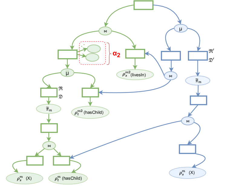
Figure 11. Expansion of a RLQDAG by pushing a join in a fixpoint operation node. The initial RLQDAG is in green color, and parts added by $\text{pj}()$ are in blue color.

Merging fixpoint operation nodes

The function $\text{mf}()$ defined in Fig. 12 takes an input $\gamma$ and returns an equivalence node $\gamma^{\prime}$ containing all the subterms in $\gamma$ with, in addition, all the terms in which recursions that can be merged are merged. A merging happens whenever (i) two recursions are joined and (ii) their annotated equivalence nodes allow them to be merged into a single recursion, as described in Fig. 12. The constant part of the new recursive term created is the join of the constant parts of the two initial fixpoints, and a new recursive part is created. Since the constant part has changed, a new recursive variable is introduced and recursive parts are also new (and cannot be shared).

For example, the query $\mathcal{Q}_{e_{4}}$:

$\footnotesize?s,~{}?t~{}~{}\leftarrow~{}~{}?s~{}~{}\texttt{islocatedin+/dealswith+}~{}~{}?t$

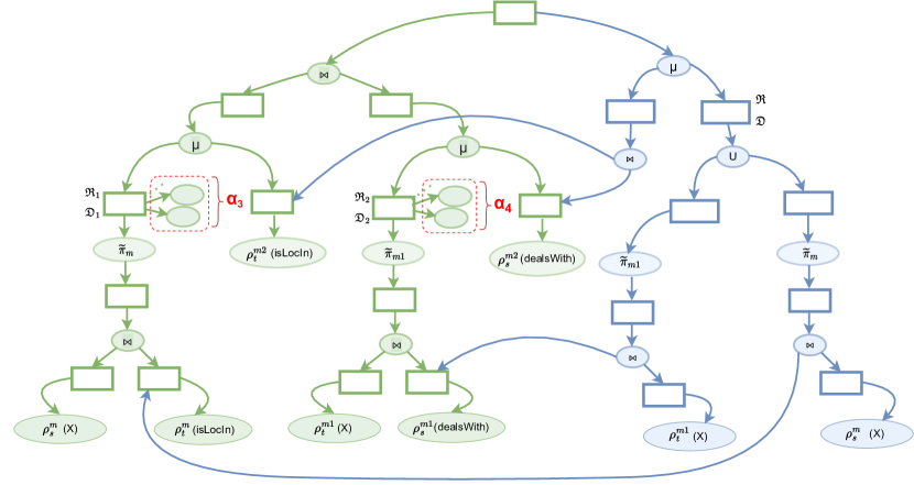
Figure 13. RLQDAG structure after merging fixpoint operation nodes.

retrieves all pairs of nodes that are connected by a path composed of two successive sequences of edges labeled islocatedin and dealswith respectively. Fig. 13 illustrates a portion of $\mathcal{Q}_{e_{4}}$ RLQDAG, with the new recursive term produced, using subterm-sharing, after the merging of fixpoint operation nodes.

$\text{mf}(\bm{\bigr{[}}~{}{\bm{\bigr{[}}\mu X_{1}.~{}\gamma_{1}~{}\cup~{}\bm{\bigr{[}}\alpha_{1}\bm{\bigr{]}}_{\mathfrak{D_{1}}}^{\mathfrak{R_{1}}}\bm{\bigr{]}}}\bowtie{\bm{\bigr{[}}\mu X_{2}.~{}\gamma_{2}~{}\cup~{}\bm{\bigr{[}}\alpha_{2}\bm{\bigr{]}}_{\mathfrak{D_{2}}}^{\mathfrak{R_{2}}}\bm{\bigr{]}}}~{}\bm{\bigr{]}}~{})=\newline \mbox{ }~{}\hskip 19.91684pt\left\{\begin{array}[]{ll}\mathbin{\vbox{\hbox{\scalebox{1.1}{$\bullet$}}}}&\text{let $\text{const}_{1}$}=\gamma_{1}~{}\text{in}\\ &\text{let $\text{const}_{2}$}=\gamma_{2}~{}\text{in}\\ &\quad~{}\bm{\bigr{[}}~{}\texttt{expand}(\bm{\bigr{[}}\mu X_{1}.~{}\text{const}_{1}~{}\cup~{}\bm{\bigr{[}}\alpha_{1}\bm{\bigr{]}}_{\mathfrak{D_{1}}}^{\mathfrak{R_{1}}}\bm{\bigr{]}})~{}\bowtie~{}\texttt{expand}(\bm{\bigr{[}}\mu X_{2}.~{}\text{const}_{2}~{}\cup~{}\bm{\bigr{[}}\alpha_{2}\bm{\bigr{]}}_{\mathfrak{D_{2}}}^{\mathfrak{R_{2}}}\bm{\bigr{]}})~{}~{},\\ &\quad{\color[rgb]{0,0,1}\mu X.~{}\texttt{expand}(\bm{\bigr{[}}\text{const}_{1}\bowtie\text{const}_{2}\bm{\bigr{]}})\cup~{}\texttt{expand}(\bm{\bigr{[}}{\alpha_{1}}_{\{{X_{1}}/{X}\}}~{}\cup~{}{\alpha_{2}}_{\{{X_{2}}/{X}\}}\bm{\bigr{]}}_{\mathfrak{D}}^{\mathfrak{R}}~{})}~{}~{}\bm{\bigr{]}}\\ &{{when}~{}~{}\text{$(\text{\emph{type}}{(\gamma_{1})}\cap\text{\emph{type}}{(\gamma_{2})})\cap(\mathfrak{D_{1}}\cup\mathfrak{D_{2}})=\emptyset$}~{}and~{}\text{$\text{\emph{type}}{(\gamma_{1})}\backslash\text{\emph{type}}{(\gamma_{2})}\cap\mathfrak{R_{2}}=\emptyset$}~{}and~{}\text{$\text{\emph{type}}{(\gamma_{2})}\backslash\text{\emph{type}}{(\gamma_{1})}\cap\mathfrak{R_{1}}=\emptyset$}}\\ \mathbin{\vbox{\hbox{\scalebox{1.1}{$\bullet$}}}}&\texttt{expand}(~{}\bm{\bigr{[}}\mu X_{1}.~{}\text{const}_{1}~{}\cup~{}\bm{\bigr{[}}\alpha_{1}\bm{\bigr{]}}_{\mathfrak{D_{1}}}^{\mathfrak{R_{1}}}\bm{\bigr{]}})~{}\bowtie~{}\texttt{expand}(\bm{\bigr{[}}\mu X_{2}.~{}\text{const}_{2}~{}\cup~{}\bm{\bigr{[}}\alpha_{2}\bm{\bigr{]}}_{\mathfrak{D_{2}}}^{\mathfrak{R_{2}}}\bm{\bigr{]}}~{})\qquad{otherwise}\end{array}\right.$

$\text{mf}(\bm{\bigr{[}}~{}{\bm{\bigr{[}}\mu X_{1}.~{}\gamma_{1}~{}\cup~{}\bm{\bigr{[}}\alpha_{1}\bm{\bigr{]}}_{\mathfrak{D_{1}}}^{\mathfrak{R_{1}}},\alpha_{3}\bm{\bigr{]}}}\bowtie{\bm{\bigr{[}}\mu X_{2}.~{}\gamma_{2}~{}\cup~{}\bm{\bigr{[}}\alpha_{2}\bm{\bigr{]}}_{\mathfrak{D_{2}}}^{\mathfrak{R_{2}}},\alpha_{4}\bm{\bigr{]}}}~{}\bm{\bigr{]}}~{})=\newline \mbox{ }~{}\hskip 19.91684pt\left\{\begin{array}[]{ll}\mathbin{\vbox{\hbox{\scalebox{1.1}{$\bullet$}}}}&\text{let $\text{const}_{1}$}=\gamma_{1}~{}\text{in}\\ &\text{let $\text{const}_{2}$}=\gamma_{2}~{}\text{in}\\ &\quad\bm{\bigr{[}}~{}\texttt{expand}(\bm{\bigr{[}}\mu X_{1}.~{}\text{const}_{1}~{}\cup~{}\bm{\bigr{[}}\alpha_{1}\bm{\bigr{]}}_{\mathfrak{D_{1}}}^{\mathfrak{R_{1}}}\bm{\bigr{]}})~{}\bowtie~{}\texttt{expand}(\bm{\bigr{[}}\mu X_{2}.~{}\text{const}_{2}~{}\cup~{}\bm{\bigr{[}}\alpha_{2}\bm{\bigr{]}}_{\mathfrak{D_{2}}}^{\mathfrak{R_{2}}}\bm{\bigr{]}})~{}~{},\\ &\quad{\color[rgb]{0,0,1}\mu X.~{}\texttt{expand}(\bm{\bigr{[}}\text{const}_{1}\bowtie\text{const}_{2}\bm{\bigr{]}})\cup~{}\texttt{expand}(\bm{\bigr{[}}{\alpha_{1}}_{\{{X_{1}}/{X}\}}~{}\cup~{}{\alpha_{2}}_{\{{X_{2}}/{X}\}}\bm{\bigr{]}}_{\mathfrak{D}}^{\mathfrak{R}}~{})}~{}~{},\\ &\quad\texttt{expand}(\bm{\bigr{[}}\alpha_{3}\bm{\bigr{]}})\bowtie\texttt{expand}(\bm{\bigr{[}}\mu X_{2}.~{}\gamma_{2}~{}\cup~{}\bm{\bigr{[}}\alpha_{2}\bm{\bigr{]}}_{\mathfrak{D_{2}}}^{\mathfrak{R_{2}}},\alpha_{4}\bm{\bigr{]}})~{}~{},\\ &\quad\texttt{expand}(\bm{\bigr{[}}\alpha_{4}\bm{\bigr{]}})\bowtie\texttt{expand}(\bm{\bigr{[}}\mu X_{1}.~{}\gamma_{1}~{}\cup~{}\bm{\bigr{[}}\alpha_{1}\bm{\bigr{]}}_{\mathfrak{D_{1}}}^{\mathfrak{R_{1}}},\alpha_{3}\bm{\bigr{]}})~{}~{}\bm{\bigr{]}}\\ &{{when}~{}~{}\text{$(\text{\emph{type}}{(\gamma_{1})}\cap\text{\emph{type}}{(\gamma_{2})})\cap(\mathfrak{D_{1}}\cup\mathfrak{D_{2}})=\emptyset$}~{}~{}{and}~{}~{}\text{$\text{\emph{type}}{(\gamma_{1})}\backslash\text{\emph{type}}{(\gamma_{2})}\cap\mathfrak{R_{2}}=\emptyset$}~{}~{}{and}~{}~{}\text{$\text{\emph{type}}{(\gamma_{2})}\backslash\text{\emph{type}}{(\gamma_{1})}\cap\mathfrak{R_{1}}=\emptyset$}}\\ \mathbin{\vbox{\hbox{\scalebox{1.1}{$\bullet$}}}}&\bm{\bigr{[}}~{}\texttt{expand}({{\bm{\bigr{[}}\mu X_{1}.~{}\gamma_{1}~{}\cup~{}\bm{\bigr{[}}\alpha_{1}\bm{\bigr{]}}_{\mathfrak{D_{1}}}^{\mathfrak{R_{1}}},\alpha_{3}\bm{\bigr{]}}}})\bowtie\texttt{expand}({\bm{\bigr{[}}\mu X_{2}.~{}\gamma_{2}~{}\cup~{}\bm{\bigr{[}}\alpha_{2}\bm{\bigr{]}}_{\mathfrak{D_{2}}}^{\mathfrak{R_{2}}},\alpha_{4}\bm{\bigr{]}}})~{},\\ &\texttt{expand}(\bm{\bigr{[}}\alpha_{3}\bm{\bigr{]}})\bowtie\texttt{expand}(\bm{\bigr{[}}\mu X_{2}.~{}\gamma_{2}~{}\cup~{}\bm{\bigr{[}}\alpha_{2}\bm{\bigr{]}}_{\mathfrak{D_{2}}}^{\mathfrak{R_{2}}},\alpha_{4}\bm{\bigr{]}})~{}~{},\\ &\texttt{expand}(\bm{\bigr{[}}\alpha_{4}\bm{\bigr{]}})\bowtie\texttt{expand}(\bm{\bigr{[}}\mu X_{1}.~{}\gamma_{1}~{}\cup~{}\bm{\bigr{[}}\alpha_{1}\bm{\bigr{]}}_{\mathfrak{D_{1}}}^{\mathfrak{R_{1}}},\alpha_{3}\bm{\bigr{]}})~{}~{}\bm{\bigr{]}}\qquad otherwise\end{array}\right.$

where $\mathfrak{D}=\mathfrak{D_{1}}\cup\mathfrak{D_{2}}$ and $\mathfrak{R}=\mathfrak{R_{1}}\cup\mathfrak{R_{2}}$ and ${\alpha_{i}}_{\{{X_{i}}/{X}\}}$ denotes $\alpha_{i}$ in which all occurrences of $X_{i}$ are replaced by $X$. This is because the only transformation of the recursive part that needs to be propagated to update the annotations is the union of the two former recursive parts and both destab and rigid are distributive over union.

Figure 12. Merging fixpoint operation nodes.

Pushing an antiprojection in a fixpoint operation node

$\text{pp}(\bm{\bigr{[}}~{}~{}\widetilde{\pi}_{a}~{}~{}{\bm{\bigr{[}}\mu X.~{}\gamma~{}\cup~{}\bm{\bigr{[}}\alpha\bm{\bigr{]}}_{\mathfrak{D}}^{\mathfrak{R}}\bm{\bigr{]}}}\bm{\bigr{]}})=\newline \mbox{ }~{}\hskip 8.5359pt\left\{\begin{array}[]{ll}\mathbin{\vbox{\hbox{\scalebox{1.1}{$\bullet$}}}}&\bm{\bigr{[}}~{}~{}{\color[rgb]{0,0,1}\mu X^{\prime}.~{}\text{expand}(\bm{\bigr{[}}\widetilde{\pi}_{a}({\gamma})\bm{\bigr{]}})~{}\cup~{}\bm{\bigr{[}}\texttt{expand}({\alpha}_{\{{X}/{X^{\prime}}\}})\bm{\bigr{]}}_{\mathfrak{D^{\prime}}}^{\mathfrak{R^{\prime}}}}~{}~{}\bm{\bigr{]}}\\ &{when}~{}~{}a\notin\mathfrak{R}\\ \mathbin{\vbox{\hbox{\scalebox{1.1}{$\bullet$}}}}&\bm{\bigr{[}}\widetilde{\pi}_{a}(\texttt{expand}({\bm{\bigr{[}}\mu X.~{}\gamma~{}\cup~{}\bm{\bigr{[}}\alpha\bm{\bigr{]}}_{\mathfrak{D}}^{\mathfrak{R}}\bm{\bigr{]}}}))~{}~{}\bigr{]}~{}~{}\quad{otherwise}\end{array}\right.$

$\text{pp}(\bm{\bigr{[}}~{}~{}\widetilde{\pi}_{a}~{}~{}({\bm{\bigr{[}}\mu X.~{}\gamma~{}\cup~{}\bm{\bigr{[}}\alpha\bm{\bigr{]}}_{\mathfrak{D}}^{\mathfrak{R}},\alpha_{2}\bm{\bigr{]}}})\bm{\bigr{]}})=\newline \mbox{ }~{}\hskip 8.5359pt\left\{\begin{array}[]{ll}\mathbin{\vbox{\hbox{\scalebox{1.1}{$\bullet$}}}}&\bm{\bigr{[}}~{}~{}{\color[rgb]{0,0,1}\mu X^{\prime}.~{}\text{expand}(\bm{\bigr{[}}\widetilde{\pi}_{a}({\gamma})\bm{\bigr{]}})~{}\cup~{}\bm{\bigr{[}}\texttt{expand}({\alpha}_{\{{X}/{X^{\prime}}\}})\bm{\bigr{]}}_{\mathfrak{D^{\prime}}}^{\mathfrak{R^{\prime}}}}~{},\\ &\quad\texttt{expand}(\bm{\bigr{[}}\widetilde{\pi}_{a}(\bm{\bigr{[}}\alpha_{2}\bm{\bigr{]}})\bm{\bigr{]}})~{}~{}\bm{\bigr{]}}\quad{when}~{}~{}a\notin\mathfrak{R}\\ \mathbin{\vbox{\hbox{\scalebox{1.1}{$\bullet$}}}}&\bm{\bigr{[}}~{}~{}\widetilde{\pi}_{a}(\texttt{expand}({\bm{\bigr{[}}\mu X.~{}\gamma~{}\cup~{}\bm{\bigr{[}}\alpha\bm{\bigr{]}}_{\mathfrak{D}}^{\mathfrak{R}},\alpha_{2}\bm{\bigr{]}}}))~{},\\ &~{}\texttt{expand}(\bm{\bigr{[}}\widetilde{\pi}_{a}(\bm{\bigr{[}}\alpha_{2}\bm{\bigr{]}})\bm{\bigr{]}})~{}~{}\bigr{]}\qquad{otherwise}\end{array}\right.$

where $\mathfrak{D^{\prime}}=\mathfrak{D}\cup\{a\}$ and $\mathfrak{R^{\prime}}=\mathfrak{R}\cup\{a\}$.

Figure 14. Pushing antiprojection in an equivalence node containing a fixpoint.

For pushing antiprojections into fixpoint operation nodes we introduce a function $\text{pp}()$ that takes an equivalence node $\gamma$ as input and returns an expanded equivalence node $\gamma^{\prime}$ where all pushable antiprojections have been pushed. $\text{pp}()$ is defined in Fig. 14. The antiprojection is pushed when the criteria allows it, and this results in the creation of a new term which replaces the initial one in the existing equivalence node. Whenever the criteria is not satisfied, the initial term is left unchanged, but traversed in search for more transformation opportunities.

Pushing an antijoin in a fixpoint operation node

For pushing antijoins into fixpoints we introduce a function $\text{pa}()$ that takes an equivalence node $\gamma$ as input and returns an expanded node $\gamma^{\prime}$ that contains all the subterms in $\gamma$ with, in addition, all subterms where all pushable antijoins have been pushed in fixpoint operation nodes. $\text{pa}()$ is defined in Fig. 15. Again, Fig. 15 focuses on the syntactic cases that correspond to when an antijoin might be pushed in a fixpoint. When criteria are satisfied, the antijoin is pushed in the constant part of the fixpoint operation node and the newly created term is added to the set of equivalent terms along with the rest.

RLQDAG rules can be divided into two groups. The first group is composed of rewrite rules $\text{pj}()$, $\text{pa}()$ and $\text{mf}()$. The application of these rules always preserve preexisting terms in an equivalence node. These rules can only perform additions of new operation nodes in an equivalence node. The second group is composed of the rules $\text{pf}()$ and $\text{pp}()$ that perform logical optimizations. The application of these rules can replace terms in an equivalence node by more optimal variants (i.e. they discard logically suboptimal variants).

$\text{pa}(\bm{\bigr{[}}{\bm{\bigr{[}}\mu X.~{}\gamma~{}\cup~{}\bm{\bigr{[}}\alpha\bm{\bigr{]}}_{\mathfrak{D}}^{\mathfrak{R}}\bm{\bigr{]}}}\triangleright\beta\bm{\bigr{]}})=\newline \mbox{ }~{}\hskip 2.84544pt\left\{\begin{array}[]{ll}\mathbin{\vbox{\hbox{\scalebox{1.1}{$\bullet$}}}}&\text{let const}=\gamma~{}\text{in}{}\\ &\quad\bm{\bigr{[}}~{}~{}\bm{\bigr{[}}\texttt{expand}(\bm{\bigr{[}}\mu X.~{}\text{const}~{}\cup~{}\bm{\bigr{[}}\alpha\bm{\bigr{]}}_{\mathfrak{D}}^{\mathfrak{R}}\bm{\bigr{]}})\triangleright\texttt{expand}(\beta)\bm{\bigr{]}}~{},\\ &\quad{\color[rgb]{0,0,1}\mu X^{\prime}.~{}\texttt{expand}(\bm{\bigr{[}}\text{const}\triangleright\beta\bm{\bigr{]}})~{}\cup~{}\bm{\bigr{[}}\texttt{expand}({\alpha}_{\{{X}/{X^{\prime}}\}})\bm{\bigr{]}}_{\mathfrak{D}}^{\mathfrak{R^{\prime}}}}~{}~{}\bm{\bigr{]}}\\ &{when}~{}~{}\text{\emph{type}}{(\beta)}\cap\mathfrak{D}=\emptyset\\ \mathbin{\vbox{\hbox{\scalebox{1.1}{$\bullet$}}}}&\bm{\bigr{[}}~{}~{}\texttt{expand}(\bm{\bigr{[}}\mu X.~{}\gamma~{}\cup~{}\bm{\bigr{[}}\alpha\bm{\bigr{]}}_{\mathfrak{D}}^{\mathfrak{R}}\bm{\bigr{]}})\triangleright\texttt{expand}(\beta)~{}~{}~{}\bigr{]}~{}~{}~{}{otherwise}\end{array}\right.$

$\text{pa}(\bm{\bigr{[}}{\bm{\bigr{[}}\mu X.~{}\gamma~{}\cup~{}\bm{\bigr{[}}\alpha\bm{\bigr{]}}_{\mathfrak{D}}^{\mathfrak{R}},~{}\alpha_{2}\bm{\bigr{]}}}\triangleright\beta\bm{\bigr{]}})=\newline \mbox{ }~{}\hskip 2.84544pt\left\{\begin{array}[]{ll}\mathbin{\vbox{\hbox{\scalebox{1.1}{$\bullet$}}}}&\text{let const}=\gamma~{}\text{in}{}\\ &\quad\bm{\bigr{[}}~{}~{}\bm{\bigr{[}}\texttt{expand}(\bm{\bigr{[}}\mu X.~{}\text{const}~{}\cup~{}\bm{\bigr{[}}\alpha\bm{\bigr{]}}_{\mathfrak{D}}^{\mathfrak{R}},~{}\alpha_{2}\bm{\bigr{]}})\triangleright\texttt{expand}(\beta)\bm{\bigr{]}},\\ &\quad{\color[rgb]{0,0,1}\bm{\bigr{[}}\mu X^{\prime}.~{}\texttt{expand}(\bm{\bigr{[}}\text{const}\triangleright\beta\bm{\bigr{]}})~{}\cup~{}\bm{\bigr{[}}\texttt{expand}({\alpha}_{\{{X}/{X^{\prime}}\}})\bm{\bigr{]}}_{\mathfrak{D}}^{\mathfrak{R^{\prime}}}\bm{\bigr{]}}},\\ &\quad\bm{\bigr{[}}\texttt{expand}(\bm{\bigr{[}}\alpha_{2}\bm{\bigr{]}})\triangleright\texttt{expand}(\beta)\bm{\bigr{]}}~{}~{}\bm{\bigr{]}}\\ &{when}~{}~{}\text{\emph{type}}{(\beta)}\cap\mathfrak{D}=\emptyset\\ \mathbin{\vbox{\hbox{\scalebox{1.1}{$\bullet$}}}}&\bm{\bigr{[}}~{}~{}\texttt{expand}(\bm{\bigr{[}}\mu X.~{}\gamma~{}\cup~{}\bm{\bigr{[}}\alpha\bm{\bigr{]}}_{\mathfrak{D}}^{\mathfrak{R}},~{}\alpha_{2}\bm{\bigr{]}})\triangleright\texttt{expand}(\beta),\\ &\quad\bm{\bigr{[}}\texttt{expand}(\bm{\bigr{[}}\alpha_{2}\bm{\bigr{]}})\triangleright\texttt{expand}(\beta)\bm{\bigr{]}}~{}~{}\bm{\bigr{]}}\qquad{otherwise}\end{array}\right.$ where $\mathfrak{R^{\prime}}=\mathfrak{R}\cup\texttt{rigid}(\beta,X)$.

Figure 15. Pushing antijoin in an equivalence node containing a fixpoint.

4.2. The overall expansion algorithm

We can now describe the overall RLQDAG expansion algorithm. We define the function $\texttt{expand}()$ that takes an equivalence node $\gamma$ and returns the equivalence node $\gamma^{\prime}$ which contains all the terms obtained by transformations. The expand function is simply defined as follows:

$$\footnotesize\begin{array}[]{rcl}\texttt{expand}(\bm{\bigr{[}}d\bm{\bigr{]}})&=&\texttt{applyAll}(\bm{\bigr{[}}d\bm{\bigr{]}})\\ \texttt{expand}(\bm{\bigr{[}}d,\alpha\bm{\bigr{]}})&=&\texttt{applyAll}(\bm{\bigr{[}}d\bm{\bigr{]}})\cup\texttt{expand}(\alpha)\\ \end{array}$$

where $\texttt{applyAll}()$ is in charge of applying all possible transformations on each operation node. This includes applying all rewrite rules defined in Section 4 in combination with the more classical ones of relational algebra:

$$\footnotesize\begin{array}[]{rcl}\texttt{applyAll}(\bm{\bigr{[}}d\bm{\bigr{]}})&=&\text{pf}(\bm{\bigr{[}}d\bm{\bigr{]}})\cup\text{pa}(\bm{\bigr{[}}d\bm{\bigr{]}})\cup\text{pj}(\bm{\bigr{[}}d\bm{\bigr{]}})\cup\text{mf}(\bm{\bigr{[}}d\bm{\bigr{]}})\\ &&\cup~{}\text{pp}(\bm{\bigr{[}}d\bm{\bigr{]}})\cup\texttt{allCodd}(\bm{\bigr{[}}d\bm{\bigr{]}})\\ \end{array}$$

where $\texttt{allCodd}()$ applies all rewrite rules concerning classical (non-recursive) relational algebra adapted for RLQDAG. For example: $\text{pfj}()$ for pushing filters in join operation nodes, $\text{paj}()$ for pushing antiprojections in a join operation node, $\text{jassoc}()$ (for join associativity), $\text{dju}()$ (for distributivity of join over union operation nodes) etc.

$$\footnotesize\begin{array}[]{rcl}\texttt{allCodd}(\bm{\bigr{[}}d\bm{\bigr{]}})&=&\text{pfj}(\bm{\bigr{[}}d\bm{\bigr{]}})\cup\text{paj}(\bm{\bigr{[}}d\bm{\bigr{]}})\cup\\ &&\text{jassoc}(\bm{\bigr{[}}d\bm{\bigr{]}})\cup...\cup\text{dju}(\bm{\bigr{[}}d\bm{\bigr{]}})\end{array}$$

For instance, $\text{pfj}()$ is defined as shown in Fig. 16 for an RLQDAG in which a filter precedes an equivalence node which contains a join operation node. In other cases, $\text{pfj}()$ recursively traverses the structure with appropriate calls to $\texttt{expand}()$ in search for further transformation opportunities. Other rewrite rules of non-recursive relational algebra are also implemented in a similar way in the RLQDAG.

$\text{pfj}(\bm{\bigr{[}}\sigma_{f}({\bm{\bigr{[}}\gamma_{1}\bowtie\gamma_{2},\alpha\bm{\bigr{]}}})\bm{\bigr{]}})=\newline \mbox{ }~{}\hskip 11.38092pt\left\{\begin{array}[]{ll}\mathbin{\vbox{\hbox{\scalebox{1.1}{$\bullet$}}}}&\bm{\bigr{[}}~{}{\color[rgb]{0,0,0}{\texttt{exp}({\bm{\bigr{[}}\sigma_{f}({\gamma_{1}})\bm{\bigr{]}}})\bowtie\texttt{exp}({\gamma_{2}})},~{}\texttt{exp}({\bm{\bigr{[}}\sigma_{f}({\alpha})\bm{\bigr{]}}})}~{}\bm{\bigr{]}}\\ &{when}~{}~{}\text{\emph{filt(f)}}\subseteq\text{\emph{type}}{(\gamma_{1})}\land\text{\emph{filt(f)}}\nsubseteq\text{\emph{type}}{(\gamma_{2})}\\ \mathbin{\vbox{\hbox{\scalebox{1.1}{$\bullet$}}}}&\bm{\bigr{[}}~{}{\color[rgb]{0,0,0}{\texttt{exp}({\gamma_{1}})\bowtie\texttt{exp}({\bm{\bigr{[}}\sigma_{f}({\gamma_{2}})\bm{\bigr{]}}})},~{}\texttt{exp}({\bm{\bigr{[}}\sigma_{f}({\alpha})\bm{\bigr{]}}})}~{}\bm{\bigr{]}}\\ &{when}~{}\text{\emph{filt(f)}}\nsubseteq\text{\emph{type}}{(\gamma_{1})}\land\text{\emph{filt(f)}}\subseteq\text{\emph{type}}{(\gamma_{2})}\\ \mathbin{\vbox{\hbox{\scalebox{1.1}{$\bullet$}}}}&\bm{\bigr{[}}~{}{\color[rgb]{0,0,0}{\texttt{exp}({\bm{\bigr{[}}\sigma_{f}({\gamma_{1}})\bm{\bigr{]}}})\bowtie\texttt{exp}({\bm{\bigr{[}}\sigma_{f}({\gamma_{2}})\bm{\bigr{]}}})},~{}\texttt{exp}({\bm{\bigr{[}}\sigma_{f}({\alpha})\bm{\bigr{]}}})}~{}\bm{\bigr{]}}\\ &{when}~{}\text{\emph{filt(f)}}\subseteq\text{\emph{type}}{(\gamma_{1})}\land\text{\emph{filt(f)}}\subseteq\text{\emph{type}}{(\gamma_{2})}\\ \mathbin{\vbox{\hbox{\scalebox{1.1}{$\bullet$}}}}&\bm{\bigr{[}}~{}\sigma_{f}({\texttt{exp}({\bm{\bigr{[}}\varphi\bowtie\psi\bm{\bigr{]}}}),~{}\texttt{exp}({\bm{\bigr{[}}\sigma_{f}({\alpha})\bm{\bigr{]}}})})~{}\bm{\bigr{]}}~{}~{}otherwise\end{array}\right.$

Figure 16. Pushing a filter in an equivalence node composed of at least one join operation node and other operation nodes (exp() stands for expand()).

4.3. Correctness and completeness

Proposition 1 (Correctness).

Let $\bm{\bigr{[}}\alpha\bm{\bigr{]}}$ be a consistent RLQDAG, and $\alpha^{\prime}=\texttt{expand}(\bm{\bigr{[}}\alpha\bm{\bigr{]}})$, then we have $S_{\gamma}\llbracket{\bm{\bigr{[}}\alpha\bm{\bigr{]}}}\rrbracket_{\emptyset}\subseteq S_{\gamma}\llbracket\alpha^{\prime}\rrbracket_{\emptyset}$ and $\alpha^{\prime}$ is consistent.

Proof Sketch.

The proof of correctness is done by induction on the structure of $\alpha^{\prime}$, using a case-by-case analysis of syntactic decompositions (i.e. by considering separately each RLQDAG subcase and the corresponding case of the generalized rewrite rule that applies to it). The complete formal proof is too large to be listed here (with many straightforward subcases). We summarize the main principles as well as useful auxiliary properties. When proving correctness for each RLQDAG rewrite rule, (i) we focus on each newly created recursive term added by the expansion, and (ii) use the consistency hypothesis on the recursive term before transformation to apply the theorems for individual terms of (Jachiet et al., 2020) to each rearrangement of fixpoint operation node. We also need to show that the incremental updates of annotations performed by the RLQDAG rewrite rules preserve consistency. This is done for each update by leveraging the properties that both destab () and rigid() are distributive over union. ∎

Proposition 2 (Completeness properties).

Let $R$ be a set of RLQDAG rewrite rules such that $R$ contains the 5 RLQDAG rewrite rules for recursive terms presented in Section 4, we consider $\bm{\bigr{[}}\alpha\bm{\bigr{]}}=\texttt{unfold}(\texttt{expand}_{R}(\bm{\bigr{[}}\alpha^{\prime}\bm{\bigr{]}}))$ where $\alpha^{\prime}$ is a consistent RLQDAG, and $\texttt{expand}_{R}()$ is the $\texttt{expand}()$ function in which rules in $R$ are activated. The following properties hold:

Property 1 (All pushable filters have been pushed).

$\forall~{}\sigma_{f}({\gamma})\in\bm{\bigr{[}}\alpha\bm{\bigr{]}}$, $\nexists{}d\in\gamma\mid d=\mu X.~{}\bm{\bigr{[}}\kappa\bm{\bigr{]}}\cup\bm{\bigr{[}}\alpha_{2}\bm{\bigr{]}}_{\mathfrak{D}}^{\mathfrak{R}}$ and $\text{\emph{filt(f)}}\cap\mathfrak{D}=\emptyset$.

Property 2 (All pushable antiprojections pushed).

$\forall~{}\widetilde{\pi}_{a}(\gamma)\in\bm{\bigr{[}}\alpha\bm{\bigr{]}}$, $\nexists{}d\in\gamma\mid d=\mu X.~{}\bm{\bigr{[}}\kappa\bm{\bigr{]}}\cup\bm{\bigr{[}}\alpha_{2}\bm{\bigr{]}}_{\mathfrak{D}}^{\mathfrak{R}}$ and $a\not\in\mathfrak{R}$.

Property 3 (All pushable joins pushed).

$\forall~{}({\beta}\bowtie{\gamma})\in\bm{\bigr{[}}\alpha\bm{\bigr{]}}$, if $\exists d\in\gamma$ such that $d=\mu X.~{}\bm{\bigr{[}}\kappa\bm{\bigr{]}}\cup\bm{\bigr{[}}\alpha_{2}\bm{\bigr{]}}_{\mathfrak{D}}^{\mathfrak{R}}$ and $\text{\emph{type}}{(\beta)}\cap\mathfrak{D}=\emptyset$ and $\text{\emph{type}}{(\beta)}\backslash\text{\emph{type}}{(\gamma)}\thickspace\cap\mathfrak{R}=\emptyset$ then $\exists d^{\prime}\in\bm{\bigr{[}}\alpha\bm{\bigr{]}}$ such that $d^{\prime}=\mu X^{\prime}.~{}\bm{\bigr{[}}\bm{\bigr{[}}\beta\bm{\bigr{]}}\bowtie{\bm{\bigr{[}}\kappa\bm{\bigr{]}}}\bm{\bigr{]}}\cup\bm{\bigr{[}}{\alpha_{2}}_{\{{X}/{X^{\prime}}\}}\bm{\bigr{]}}_{\mathfrak{D^{\prime}}}^{\mathfrak{R^{\prime}}}$.

Property 4 (All mergeable fixpoints merged).

$\forall~{}({\gamma_{1}}\bowtie{\gamma_{2}})\in\bm{\bigr{[}}\alpha\bm{\bigr{]}}$, if $\mu X_{1}.~{}\bm{\bigr{[}}\kappa_{1}\bm{\bigr{]}}\cup\bm{\bigr{[}}\alpha_{1}\bm{\bigr{]}}_{\mathfrak{D_{1}}}^{\mathfrak{R_{1}}}\in\gamma_{1}$ and $\mu X_{2}.~{}\bm{\bigr{[}}\kappa_{2}\bm{\bigr{]}}\cup\bm{\bigr{[}}\alpha_{2}\bm{\bigr{]}}_{\mathfrak{D_{2}}}^{\mathfrak{R_{2}}}\in\gamma_{2}$ and we have $\gamma_{1}\neq\gamma_{2}$ and $(\text{\emph{type}}{(\gamma_{1})}\cap\text{\emph{type}}{(\gamma_{2})})\cap(\mathfrak{D_{1}}\cup\mathfrak{D_{2}})=\emptyset$ and $\text{\emph{type}}{(\gamma_{1})}\backslash\text{\emph{type}}{(\gamma_{2})}\cap\mathfrak{R_{2}}=\emptyset$ and $\text{\emph{type}}{(\gamma_{2})}\backslash\text{\emph{type}}{(\gamma_{1})}\cap\mathfrak{R_{1}}=\emptyset$ then there exists $d\in\bm{\bigr{[}}\alpha\bm{\bigr{]}}$ such that $d=\mu X.~{}\bm{\bigr{[}}\bm{\bigr{[}}\kappa_{1}\bm{\bigr{]}}\bowtie{\bm{\bigr{[}}\kappa_{2}\bm{\bigr{]}}}\bm{\bigr{]}}\cup\bm{\bigr{[}}\bm{\bigr{[}}\alpha_{1}\bm{\bigr{]}}\cup\bm{\bigr{[}}\alpha_{2}\bm{\bigr{]}}\bm{\bigr{]}}_{\mathfrak{D}}^{\mathfrak{R}}$.

Property 5 (All pushable antijoins pushed).

$\forall~{}(\bm{\bigr{[}}\mu X.~{}\gamma~{}\cup~{}\bm{\bigr{[}}\alpha\bm{\bigr{]}}_{\mathfrak{D}}^{\mathfrak{R}}\bm{\bigr{]}}\triangleright\beta)\in\bm{\bigr{[}}\alpha\bm{\bigr{]}}$, if $\text{\emph{type}}{(\beta)}\cap\mathfrak{D}=\emptyset$ then $\exists d\in\bm{\bigr{[}}\alpha\bm{\bigr{]}}$ such that $d=\bm{\bigr{[}}\mu X^{\prime}.~{}\bm{\bigr{[}}\gamma\triangleright\beta\bm{\bigr{]}}~{}\cup~{}\bm{\bigr{[}}{\alpha}_{\{{X}/{X^{\prime}}\}}\bm{\bigr{]}}_{\mathfrak{D}}^{\mathfrak{R^{\prime}}}\bm{\bigr{]}}$

Proof Sketch.

These properties are proved by contradiction: (i) assuming the existence of a missed transformation opportunity in the expansion, which (ii) necessarily implies some unrealized rule application (whereas the rule was applicable), and (iii) showing that the systematic structure traversal performed by $\texttt{expand}_{R}()$ leaves no room for such a missed opportunity, thus (iv) leading to a contradiction. ∎

5. Experimental Results

We evaluate the RLQDAG experimentally. Our assessment is driven by the following research questions:

• RQ1 How efficient is RLQDAG exploration of recursive plan spaces compared to the state-of-the-art?

• RQ2 How relevant are explorations of large recursive plan spaces for practical query evaluation?

In the following subsections we first introduce the experimental setup and the experimental methodology with chosen baselines and metrics. We then report on the results and the main lessons learned.

5.1. Experimental setup

Datasets

We consider various datasets, graphs and trees, real and generated, as described in Table 1.

Dataset	#nodes & #edges	Type	Nature
Yago (YAGO, 2019)	42M & 62M	Knowledge graph	Real
Bahamas Leaks (Bahamas-Leaks, 2016)	202K & 249K	Property graph	Real
Airbnb (Airbnb, 2022)	24K & 14K	Property graph	Real
LDBC (Boncz, 2013)	908K & 1.9M	Property graph	Synthetic
Wikitree (Fire and Elovici, 2015)	9.1M & 1.3M	Tree	Real
Academic tree (Liénard et al., 2018)	765K & 1.5M	Tree	Real

Table 1. Datasets (available from (Tyrex-repository, 2023)).

Queries

We consider a variety of recursive queries formulated against these datasets. Queries for Yago are mainly third-party regular path queries already considered in earlier papers in the literature, and chosen because they are representative of the variety of possible recursive optimizations that can apply to them. Queries over the Airbnb dataset are inspired from (Sharma et al., 2021). We added more queries formulated over the Bahamas and LDBC datasets. We consider non-regular queries (variants of same generation, and aⁿbⁿ) for the Wikitree and Academic Tree datasets. Queries and datasets used in experiments are available at (Tyrex-repository, 2023).

Hardware

All experiments are conducted on a machine with an Intel Xeon 2.20GHz CPU and 192Gb of RAM.

5.2. RQ1: Efficiency of plan space exploration.

To answer RQ1, we implemented a prototype of the RLQDAG and compare it with MuEnum, which is the plan enumerator of the state-of-the-art $\mu$-RA system (Jachiet et al., 2020). As described in Section 2, this system is of the most advanced relational-based system for recursive query optimization; providing the richest plan spaces for recursive terms. MuEnum (Jachiet et al., 2020) explores them using a state-of-the-art dynamic programming strategy, in which terms are made unique in memory so as to obtain very efficient term equality tests.

We measure the enumeration capability of the RLQDAG in terms of the number of plans explored per second for each query. We compare the performance of our RLQDAG prototype implementation with the performance of MuEnum. Figures 17, 18, 19, and Fig. 20 respectively show the results obtained for the queries over each dataset.

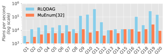
Figure 17. Yago queries.

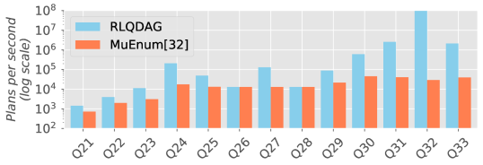
Figure 18. Bahamas Leaks queries.

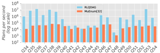
Figure 19. Airbnb and LDBC queries.

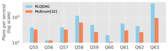
Figure 20. Non-regular queries.

In these figures, the $y$ axis (in log scale) indicates the number of plans per second explored by each approach for a given query (on the $x$ axis). Results suggest that the RLQDAG approach always enumerates plans much faster (up to two orders of magnitude) when compared to MuEnum.

Now, we set a time budget $t$ (in seconds) for the plan space exploration and let the two systems generate plan spaces for that time budget. This means that after $t$ elapsed seconds we stop the two explorations and look at the plan spaces obtained by the two systems. Fig. 21 shows the results obtained for a time budget of $t=0.5$ seconds with queries from Bahamas Leaks (Q31-Q32), Airbnb (Q34-Q37-Q38-Q39) and LDBC (Q51-Q53-Q54). The $y$ axis (in log scale) indicates the number of plans found. Fig. 21 also indicates the size of the complete (exhaustive) plan space obtained without any time restriction for the plan exploration ($t=\infty$). For example, for query Q31, the complete plan space contains more than 21.4 million plans. In 0.5 seconds, the RLQDAG prototype explored 1,019,026 plans whereas MuEnum explored only 5,751 plans. This is because although MuEnum uses dynamic programming techniques, it is not capable of benefitting from the RLQDAG’s grouping effect when applying complex rewrite rules on sets of recursive terms at once, thus rules are significantly more costly to apply. Seen from another perspective, this means that the RLQDAG’s approach is more effective in avoiding redundant subcomputations. We have conducted extensive experiments and overall results indicate that, for a given time budget, the RLQDAG prototype explores many more terms in comparison to MuEnum, in all cases. In some cases, the RLQDAG generates a number of plans which is greater by up to two orders of magnitude (for the same time budget). Such a speedup sometimes enables a complete exploration of the whole plan space in some cases (as shown e.g. for Q34, Q51, Q53, Q54 in Fig. 21).

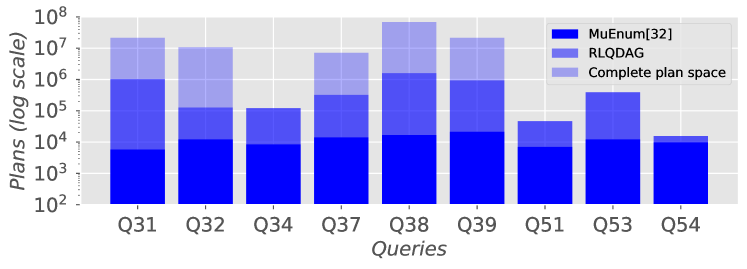
Figure 21. Plan spaces explored in 500ms.

We now report on experiments of exploring plan spaces with varying and increasing time budgets for the same query. For instance, Fig. 22 presents the number of plans explored (on the $y$ axis) for different time budgets shown on the $x$ axis for query Q31 and query Q53 (2 queries from 2 different datasets).

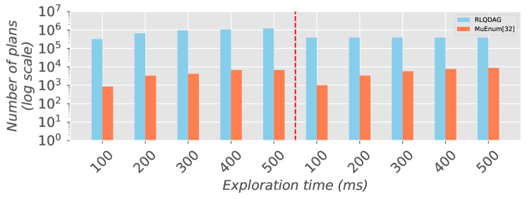
Figure 22. Plans explored per time budgets for Q31 and Q53.

Again, results shown in Fig. 22 indicate that the RLQDAG explores significantly more plans than the other approach for all considered time budgets (the $y$ axis is in log scale). We can also observe that the difference between the amount of plans explored by each system stays of the same order, even when exploration time increases.

5.3. RQ2: Relevance of exploring large plan spaces.

To answer RQ2, we use the same backend (PostgreSQL) in order to execute query plans generated by MuEnum and RLQDAG. For a given query, we set a time budget for plan space exploration, and we let MuEnum and RLQDAG generate plan spaces for this same time budget. Now, we pick the best estimated plan from each generated plan space. We use the same heuristics for cost estimations (Lawal et al., 2020), thus making relevant a head to head comparison. We measure and compare the times spent by PostgreSQL for evaluating the plans.

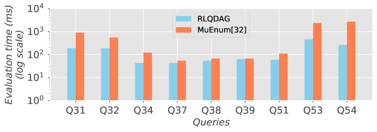
Figure 23. Evaluating best estimated plans found in explored spaces of Fig 21.

For example, Fig. 23 illustrates the time spent in evaluating the best estimated plan taken from each of the explored plan spaces reported in Fig. 21. Results show the benefits of exploring a much larger plan space: the RLQDAG approach always provides similar or better performance, which is a direct consequence of the availability of more efficient recursive plans in the larger plan space explored.

Furthermore, for the same query, we also measure the time spent in evaluating the best estimated plans from the different plan spaces explored with a varying time budget. For instance, Fig. 24 shows the time spent in evaluating the best plans selected from each plan space explored with the time budget shown on the $x$ axis. The sizes of the corresponding plan spaces are given in Fig. 22. Results shown in Fig. 24 show that the best estimated term selected from the larger plan space is more efficiently evaluated. This suggests that in practice, larger plan spaces are very prone to contain more efficient recursive plans. This confirms the interest of efficiently exploring large recursive plan spaces.

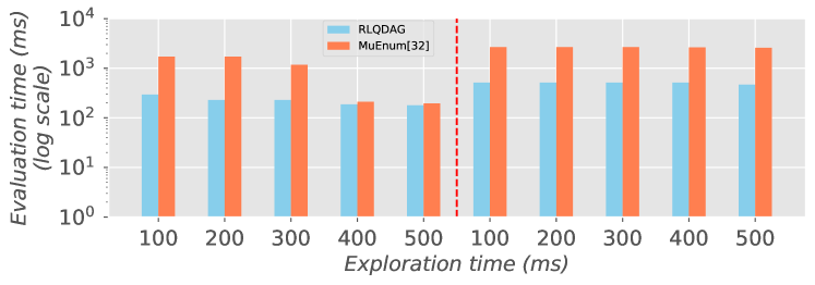
Figure 24. Evaluating best estimated plans found in explored spaces of Fig 22.

Finally, we assess to which extent the availability of more relational algebraic plans can be useful in practice, when compared to other RDBMS and state-of-the-art approaches in graph query evaluation. For this purpose, we consider 2 engines based on relational algebra (MuEnum (Jachiet et al., 2020) and Virtuoso (Erling, 2012) version 7.2.6.1), 3 native graph database engines (MilleniumDB (Vrgoč et al., 2022), Neo4j (Webber, 2012) version 4.4.11, Blazegraph (Thompson et al., 2016) version 2.1.6), and 3 plain-vanilla RDBMS capable of evaluating recursive SQL queries (PostgreSQL (Stonebraker and Rowe, 1986) version 15.1, MySQL (mys, 2023) version 8.1.0, SQLite (Hipp, 2023) version 3.36.0). We measure the time spent in query evaluation with each system. For each system, this includes the time spent in query optimization and the time spent in retrieving the whole set of query results. We set a timeout of 600s (10 min). Fig. 25 shows the corresponding times spent for systems which were able to answer. If a system does not answer before the timeout, we consider that it is unable to answer, and it is absent from Fig. 25 for the given query.

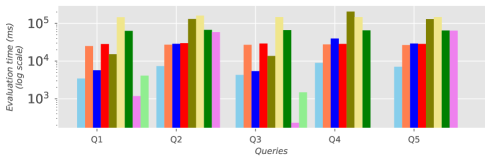
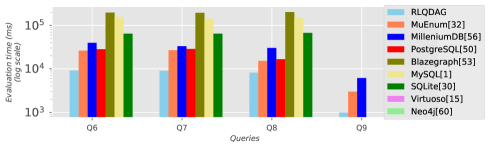
Figure 25. Comparative evaluation of third-party queries (excerpt from (Tyrex-repository, 2023)).

Results suggest that the availability of more plans – thanks to the RLQDAG – is beneficial to the relational-based approach. More specifically, existing RDBMS consider recursive queries in a very restricted way. Most of them optimize recursion-free subexpressions, without being able to optimize the recursive part as a whole: they cannot make significant structural changes to the entire recursive query. This has an important consequence: they do explore much smaller plan spaces when compared to RLQDAG, potentially missing very efficient plans. In some cases, it even makes the relational-based approach more efficient than specialized graph engines.

6. Conclusion and perspectives

We propose the RLQDAG for capturing and efficiently transforming sets of recursive relational terms. This is done by introducing annotated equivalence nodes, and a formal syntax and semantics for RLQDAG terms that enable the development of RLQDAG rewrite rules on a solid ground. RLQDAG rewrite rules transform sets of recursive terms while precisely describing how new subterms are created, attached, shared, and how new structural annotations are obtained with incremental updates. The proposed formalisation of the RLQDAG in terms of syntax and semantics provided a convenient – if not instrumental – means to develop transformations. It helps in defining expansions, and for detecting and fixing intricate transformational issues. We believe that this formalization can also serve in further extensions, thus contributing to the extensibility of the top-down transformational approach. Practical experiments with the RLQDAG show the interest of exploring large plan spaces, and suggest that it represents an interesting foundation for efficiently enumerating recursive relational query plans.

References

- (1)
- mys (2023) 2023. MySQL. https://www.mysql.com/.
- Abiteboul et al. (1995) Serge Abiteboul, Richard Hull, and Victor Vianu. 1995. Foundations of Databases: The Logical Level (1st ed.). Addison-Wesley Longman Publishing Co., Inc., USA.
- Abul-Basher et al. (2017) Zahid Abul-Basher, Nikolay Yakovets, Parke Godfrey, Shadi Ghajar-Khosravi, and Mark H Chignell. 2017. Tasweet: optimizing disjunctive regular path queries in graph databases. In EDBT/ICDT 2017 joint conference 20th international conference on extending database technology. https://doi. org/10.5441/002/edbt.
- Agrawal (1988) R. Agrawal. 1988. Alpha: an extension of relational algebra to express a class of recursive queries. IEEE Transactions on Software Engineering 14, 7 (July 1988), 879–885. https://doi.org/10.1109/32.42731
- Aho and Ullman (1979) Alfred V. Aho and Jeffrey D. Ullman. 1979. Universality of Data Retrieval Languages. In Proceedings of the 6th ACM SIGACT-SIGPLAN Symposium on Principles of Programming Languages (San Antonio, Texas) (POPL ’79). ACM, New York, NY, USA, 110–119. https://doi.org/10.1145/567752.567763
- Airbnb (2022) Airbnb. 2022. Airbnb. http://insideairbnb.com/get-the-data.html.
- Alvaro et al. (2010) Peter Alvaro, William Marczak, Neil Conway, Joseph Hellerstein, David Maier, and Russell Sears. 2010. Dedalus: Datalog in Time and Space. 262–281.
- Bahamas-Leaks (2016) Bahamas-Leaks. 2016. Bahamas Leaks. https://offshoreleaks.icij.org/pages/about.
- Bancilhon et al. (1985) Francois Bancilhon, David Maier, Yehoshua Sagiv, and Jeffrey D Ullman. 1985. Magic Sets and Other Strange Ways to Implement Logic Programs (Extended Abstract). In Proceedings of the Fifth ACM SIGACT-SIGMOD Symposium on Principles of Database Systems (Cambridge, Massachusetts, USA) (PODS ’86). Association for Computing Machinery, New York, NY, USA, 1–15. https://doi.org/10.1145/6012.15399
- Bancilhon and Ramakrishnan (1986) Francois Bancilhon and Raghu Ramakrishnan. 1986. An Amateur’s Introduction to Recursive Query Processing Strategies. In Proceedings of the 1986 ACM SIGMOD International Conference on Management of Data (Washington, D.C., USA) (SIGMOD ’86). Association for Computing Machinery, New York, NY, USA, 16–52. https://doi.org/10.1145/16894.16859
- Boncz (2013) Peter Boncz. 2013. LDBC: Benchmarks for Graph and RDF Data Management. In Proceedings of the 17th International Database Engineering ; Applications Symposium (Barcelona, Spain) (IDEAS ’13). Association for Computing Machinery, New York, NY, USA, 1–2. https://doi.org/10.1145/2513591.2527070
- Chaudhuri (1998) Surajit Chaudhuri. 1998. An Overview of Query Optimization in Relational Systems. In Proceedings of the Seventeenth ACM SIGACT-SIGMOD-SIGART Symposium on Principles of Database Systems (Seattle, Washington, USA) (PODS ’98). Association for Computing Machinery, New York, NY, USA, 34–43. https://doi.org/10.1145/275487.275492
- Chaudhuri and Shim (1994) Surajit Chaudhuri and Kyuseok Shim. 1994. Including group-by in query optimization. In VLDB, Vol. 94. 12–15.
- Codd (1970) E. F. Codd. 1970. A Relational Model of Data for Large Shared Data Banks. Commun. ACM 13, 6 (June 1970), 377–387. https://doi.org/10.1145/362384.362685
- Erling (2012) Orri Erling. 2012. Virtuoso, a Hybrid RDBMS/Graph Column Store. IEEE Data Eng. Bull. 35 (2012), 3–8.
- Fan et al. (2019) Zhiwei Fan, Jianqiao Zhu, Zuyu Zhang, Aws Albarghouthi, Paraschos Koutris, and Jignesh M. Patel. 2019. Scaling-Up In-Memory Datalog Processing: Observations and Techniques. Proc. VLDB Endow. 12, 6 (2019), 695–708. https://doi.org/10.14778/3311880.3311886
- Fender and Moerkotte (2013a) Pit Fender and Guido Moerkotte. 2013a. Counter Strike: Generic Top-down Join Enumeration for Hypergraphs. Proc. VLDB Endow. 6, 14 (sep 2013), 1822–1833. https://doi.org/10.14778/2556549.2556565
- Fender and Moerkotte (2013b) Pit Fender and Guido Moerkotte. 2013b. Top down plan generation: From theory to practice. In 2013 IEEE 29th International Conference on Data Engineering (ICDE). 1105–1116. https://doi.org/10.1109/ICDE.2013.6544901
- Fire and Elovici (2015) Michael Fire and Yuval Elovici. 2015. Data mining of online genealogy datasets for revealing lifespan patterns in human population. ACM Transactions on Intelligent Systems and Technology (TIST) 6, 2 (2015), 28.
- Francis-Landau et al. (2020) Matthew Francis-Landau, Tim Vieira, and Jason Eisner. 2020. Evaluation of Logic Programs with Built-Ins and Aggregation: A Calculus for Bag Relations.
- Galindo-Legaria and Rosenthal (1992) César Galindo-Legaria and Arnon Rosenthal. 1992. How to extend a conventional optimizer to handle one-and two-sided outerjoin. In 1992 Eighth International Conference on Data Engineering. IEEE Computer Society, 402–403.
- Galindo-Legaria and Rosenthal (1997) Cesar Galindo-Legaria and Arnon Rosenthal. 1997. Outerjoin simplification and reordering for query optimization. ACM Transactions on Database Systems (TODS) 22, 1 (1997), 43–74.
- Gardarin (1987) Georges Gardarin. 1987. Magic Functions: A Technique to Optimize Extended Datalog Recursive Programs. 21–30.
- Goldman and Widom (1997) Roy Goldman and Jennifer Widom. 1997. Dataguides: Enabling query formulation and optimization in semistructured databases. Technical Report. Stanford.
- Graefe (1995) Goetz Graefe. 1995. The Cascades Framework for Query Optimization. Data Engineering Bulletin 18 (1995).
- Graefe and DeWitt (1987) Goetz Graefe and David J. DeWitt. 1987. The EXODUS Optimizer Generator. In Proceedings of the 1987 ACM SIGMOD International Conference on Management of Data (San Francisco, California, USA) (SIGMOD ’87). ACM, New York, NY, USA, 160–172. https://doi.org/10.1145/38713.38734
- Graefe and McKenna (1993) Goetz Graefe and William J. McKenna. 1993. The Volcano Optimizer Generator: Extensibility and Efficient Search. In Proceedings of the Ninth International Conference on Data Engineering. IEEE Computer Society, Washington, DC, USA, 209–218. http://dl.acm.org/citation.cfm?id=645478.757691
- Gubichev et al. (2013) Andrey Gubichev, Srikanta J Bedathur, and Stephan Seufert. 2013. Sparqling kleene: fast property paths in RDF-3X. In First International Workshop on Graph Data Management Experiences and Systems. 1–7.
- Haas et al. (1989) L. M. Haas, J. C. Freytag, G. M. Lohman, and H. Pirahesh. 1989. Extensible Query Processing in Starburst. In Proceedings of the 1989 ACM SIGMOD International Conference on Management of Data (Portland, Oregon, USA) (SIGMOD ’89). Association for Computing Machinery, New York, NY, USA, 377–388. https://doi.org/10.1145/67544.66962
- Hipp (2023) Richard D Hipp. 2023. SQLite. https://www.sqlite.org.
- Huang et al. (2011) Shan Shan Huang, Todd Jeffrey Green, and Boon Thau Loo. 2011. Datalog and Emerging Applications: An Interactive Tutorial. In Proceedings of the 2011 ACM SIGMOD International Conference on Management of Data (Athens, Greece) (SIGMOD ’11). Association for Computing Machinery, New York, NY, USA, 1213–1216. https://doi.org/10.1145/1989323.1989456
- Jachiet et al. (2020) Louis Jachiet, Pierre Genevès, Nils Gesbert, and Nabil Layaïda. 2020. On the Optimization of Recursive Relational Queries: Application to Graph Queries. In Proceedings of the ACM SIGMOD International Conference on Management of Data. 681–697. https://doi.org/10.1145/3318464.3380567
- Kifer and Lozinskii (1990) Michael Kifer and Eliezer L. Lozinskii. 1990. On Compile-Time Query Optimization in Deductive Databases by Means of Static Filtering. ACM Trans. Database Syst. 15, 3 (sep 1990), 385–426. https://doi.org/10.1145/88636.87121
- Koschmieder and Leser (2012) André Koschmieder and Ulf Leser. 2012. Regular path queries on large graphs. In International Conference on Scientific and Statistical Database Management. Springer, 177–194.
- Lawal et al. (2020) Muideen Lawal, Pierre Genevès, and Nabil Layaïda. 2020. A Cost Estimation Technique for Recursive Relational Algebra. Proceedings of the 29th ACM International Conference on Information & Knowledge Management (2020).
- Liénard et al. (2018) Jean F Liénard, Titipat Achakulvisut, Daniel E Acuna, and Stephen V David. 2018. Intellectual synthesis in mentorship determines success in academic careers. Nature communications 9, 1 (2018), 1–13.
- Lohman (1988) Guy M. Lohman. 1988. Grammar-like Functional Rules for Representing Query Optimization Alternatives. SIGMOD Rec. 17, 3 (June 1988), 18–27. https://doi.org/10.1145/971701.50204
- Lohman et al. (1985) Guy M. Lohman, C. Mohan, Laura M. Haas, Dean Daniels, Bruce G. Lindsay, Patricia G. Selinger, and Paul F. Wilms. 1985. Query Processing in R*. Springer Berlin Heidelberg, Berlin, Heidelberg, 31–47. https://doi.org/10.1007/978-3-642-82375-6_2
- Moerkotte et al. (2013) Guido Moerkotte, Pit Fender, and Marius Eich. 2013. On the correct and complete enumeration of the core search space. In Proceedings of the 2013 ACM SIGMOD International Conference on Management of Data. 493–504.
- Naughton et al. (1989) J. F. Naughton, R. Ramakrishnan, Y. Sagiv, and J. D. Ullman. 1989. Efficient Evaluation of Right-, Left-, and Multi-Linear Rules. In Proceedings of the 1989 ACM SIGMOD International Conference on Management of Data (Portland, Oregon, USA) (SIGMOD ’89). Association for Computing Machinery, New York, NY, USA, 235–242. https://doi.org/10.1145/67544.66948
- Roy et al. (2000) Prasan Roy, S. Seshadri, S. Sudarshan, and Siddhesh Bhobe. 2000. Efficient and Extensible Algorithms for Multi Query Optimization. SIGMOD Rec. 29, 2 (May 2000), 249–260. https://doi.org/10.1145/335191.335419
- Saccà and Zaniolo (1985) Domenico Saccà and Carlo Zaniolo. 1985. On the Implementation of a Simple Class of Logic Queries for Databases. In Proceedings of the Fifth ACM SIGACT-SIGMOD Symposium on Principles of Database Systems (Cambridge, Massachusetts, USA) (PODS ’86). Association for Computing Machinery, New York, NY, USA, 16–23. https://doi.org/10.1145/6012.6013
- Schleich et al. (2023) Maximilian Schleich, Amir Shaikhha, and Dan Suciu. 2023. Optimizing Tensor Programs on Flexible Storage. Proc. ACM Manag. Data 1, 1 (2023), 37:1–37:27. https://doi.org/10.1145/3588717
- Selinger et al. (1979) P. Griffiths Selinger, M. M. Astrahan, D. D. Chamberlin, R. A. Lorie, and T. G. Price. 1979. Access Path Selection in a Relational Database Management System. In Proceedings of the 1979 ACM SIGMOD International Conference on Management of Data (Boston, Massachusetts) (SIGMOD ’79). ACM, New York, NY, USA, 23–34. https://doi.org/10.1145/582095.582099
- Seo et al. (2015) Jiwon Seo, Stephen Guo, and Monica S. Lam. 2015. SociaLite: An Efficient Graph Query Language Based on Datalog. IEEE Transactions on Knowledge and Data Engineering 27, 7 (2015), 1824–1837. https://doi.org/10.1109/TKDE.2015.2405562
- Shanbhag and Sudarshan (2014) Anil Shanbhag and S. Sudarshan. 2014. Optimizing Join Enumeration in Transformation-Based Query Optimizers. Proc. VLDB Endow. 7, 12 (aug 2014), 1243–1254. https://doi.org/10.14778/2732977.2732997
- Shapiro et al. (2001) Leonard Shapiro, David Maier, Paul Benninghoff, Keith Billings, Yubo Fan, Kavita Hatwal, Quan Wang, Yu Zhang, H.-M Wu, and Bennet Vance. 2001. Exploiting Upper and Lower Bounds in Top-Down Query Optimization. 20 – 33. https://doi.org/10.1109/IDEAS.2001.938068
- Sharma et al. (2021) Chandan Sharma, Roopak Sinha, and Kenneth Johnson. 2021. Practical and comprehensive formalisms for modelling contemporary graph query languages. Information Systems 102 (2021), 101816. https://doi.org/10.1016/j.is.2021.101816
- Shkapsky et al. (2016) Alexander Shkapsky, Mohan Yang, Matteo Interlandi, Hsuan Chiu, Tyson Condie, and Carlo Zaniolo. 2016. Big Data Analytics with Datalog Queries on Spark. In Proceedings of the 2016 International Conference on Management of Data (San Francisco, California, USA) (SIGMOD ’16). Association for Computing Machinery, New York, NY, USA, 1135–1149. https://doi.org/10.1145/2882903.2915229
- Stonebraker and Rowe (1986) Michael Stonebraker and Lawrence A. Rowe. 1986. The Design of POSTGRES (SIGMOD ’86). Association for Computing Machinery, New York, NY, USA, 340–355.
- Tate et al. (2011) Ross Tate, Michael Stepp, Zachary Tatlock, and Sorin Lerner. 2011. Equality Saturation: A New Approach to Optimization. Log. Methods Comput. Sci. 7, 1 (2011). https://doi.org/10.2168/LMCS-7(1:10)2011
- Tekle and Liu (2011) K. Tuncay Tekle and Yanhong A. Liu. 2011. More Efficient Datalog Queries: Subsumptive Tabling Beats Magic Sets. In Proceedings of the 2011 ACM SIGMOD International Conference on Management of Data (Athens, Greece) (SIGMOD ’11). Association for Computing Machinery, New York, NY, USA, 661–672. https://doi.org/10.1145/1989323.1989393
- Thompson et al. (2016) Bryan Thompson, Mike Personick, and Martyn Cutcher. 2016. The Bigdata® RDF graph database. In Linked Data Management. Chapman and Hall/CRC, 221–266.
- Tyrex-repository (2023) Tyrex-repository. 2023. Datasets and Queries used in experiments with the RLQDAG. https://gitlab.inria.fr/tyrex-public/rlqdag.
- Vianu (2021) Victor Vianu. 2021. Datalog Unchained. In PODS’21: Proceedings of the 40th ACM SIGMOD-SIGACT-SIGAI Symposium on Principles of Database Systems, Virtual Event, China, June 20-25, 2021, Leonid Libkin, Reinhard Pichler, and Paolo Guagliardo (Eds.). ACM, 57–69. https://doi.org/10.1145/3452021.3458815
- Vrgoč et al. (2022) Domagoj Vrgoč, Carlos Rojas, Renzo Angles, Marcelo Arenas, Diego Arroyuelo, Carlos Buil-Aranda, Aidan Hogan, Gonzalo Navarro, Cristian Riveros, and Juan Romero. 2022. MillenniumDB: An Open-Source Graph Database System. Data Intelligence (2022), 1–39.
- Wang et al. (2015) Jingjing Wang, Magdalena Balazinska, and Daniel Halperin. 2015. Asynchronous and Fault-Tolerant Recursive Datalog Evaluation in Shared-Nothing Engines. Proc. VLDB Endow. 8, 12 (aug 2015), 1542–1553. https://doi.org/10.14778/2824032.2824052
- Wang et al. (2020) Yisu Remy Wang, Shana Hutchison, Dan Suciu, Bill Howe, and Jonathan Leang. 2020. SPORES: Sum-Product Optimization via Relational Equality Saturation for Large Scale Linear Algebra. Proc. VLDB Endow. 13, 11 (2020), 1919–1932. http://www.vldb.org/pvldb/vol13/p1919-wang.pdf
- Wang et al. (2022) Yisu Remy Wang, Mahmoud Abo Khamis, Hung Q Ngo, Reinhard Pichler, and Dan Suciu. 2022. Optimizing Recursive Queries with Program Synthesis. arXiv preprint arXiv:2202.10390 (2022).
- Webber (2012) Jim Webber. 2012. A Programmatic Introduction to Neo4j. In Proceedings of the 3rd Annual Conference on Systems, Programming, and Applications: Software for Humanity (Tucson, Arizona, USA) (SPLASH ’12). Association for Computing Machinery, New York, NY, USA, 217–218. https://doi.org/10.1145/2384716.2384777
- Willsey et al. (2021) Max Willsey, Chandrakana Nandi, Yisu Remy Wang, Oliver Flatt, Zachary Tatlock, and Pavel Panchekha. 2021. egg: Fast and extensible equality saturation. Proc. ACM Program. Lang. 5, POPL (2021), 1–29. https://doi.org/10.1145/3434304
- YAGO (2019) YAGO. 2019. YAGO: A high-quality knowledge base. https://www.mpi-inf.mpg.de/yago-naga/yago/.
- Yakovets et al. (2015) Nikolay Yakovets, Parke Godfrey, and Jarek Gryz. 2015. WAVEGUIDE: Evaluating SPARQL Property Path Queries.. In EDBT, Vol. 2015. 525–528.
- Zauner et al. (2010) Harald Zauner, Benedikt Linse, Tim Furche, and François Bry. 2010. A RPL through RDF: Expressive navigation in RDF graphs. In International Conference on Web Reasoning and Rule Systems. Springer, 251–257.