Almost Dominance: Inference and Application

Abstract

This paper proposes a general framework for inference on three types of almost dominances: Almost Lorenz dominance, almost inverse stochastic dominance, and almost stochastic dominance. We first generalize almost Lorenz dominance to almost upward and downward Lorenz dominances. We then provide a bootstrap inference procedure for the Lorenz dominance coefficients, which measure the degrees of almost Lorenz dominances. Furthermore, we propose almost upward and downward inverse stochastic dominances and provide inference on the inverse stochastic dominance coefficients. We also show that our results can easily be extended to almost stochastic dominance. Simulation studies demonstrate the finite sample properties of the proposed estimators and the bootstrap confidence intervals. We apply our methods to the inequality growth in the United Kingdom and find evidence for almost upward inverse stochastic dominance.

Keywords: Almost Lorenz dominance, almost inverse stochastic dominance, almost stochastic dominance, estimation and inference, bootstrap confidence intervals

1 Introduction

Suppose that there are two arbitrary cumulative distribution functions (CDFs) $F_{1}:[0,\infty)\to[0,1]$ and $F_{2}:[0,\infty)\to[0,1]$ of two income (or wealth, etc.) distributions in two populations. As introduced in atkinson1970measurement, a Lorenz curve is a function that graphs the cumulative proportion of total income received by the bottom population. The distribution $F_{1}$ (weakly) Lorenz dominates $F_{2}$ if the Lorenz curve $L_{1}$ associated with $F_{1}$ is everywhere above the Lorenz curve $L_{2}$ associated with $F_{2}$. Such Lorenz dominance implies that the wealth is distributed more equally in population $F_{1}$ compared to $F_{2}$. Statistical tests of Lorenz dominance can be found in, for example, mcfadden1989testing, bishop1991international, bishop1991lorenz, dardanoni1999inference, davidson2000statistical, barrett2003consistent, BDB14, and Beare2017improved.

zheng2018almost introduces the notion of almost Lorenz dominance: When two Lorenz curves cross, $F_{1}$ almost Lorenz dominates $F_{2}$ if $L_{1}$ is above $L_{2}$ almost everywhere. The degree of almost Lorenz dominance can be measured by a coefficient, Lorenz dominance coefficient (LDC). The LDC was first proposed in zheng2018almost, which is similar to the violation ratio in huang2021estimating. zheng2018almost shows that almost Lorenz dominance is highly related to Gini-type measures. Based on the seminal work of aaberge2009ranking, we generalize almost Lorenz dominance to almost upward Lorenz dominance and almost downward Lorenz dominance. We relate the generalized LDCs to a class of inequality measures. It is straightforward to show that the smaller LDCs are, the more inequality measures demonstrate higher distribution equality in the dominant population. Thus, LDCs are of interest to us when we compare distributions in terms of distribution inequality. We then provide estimators for LDCs and establish the asymptotic properties of the estimators. Based on the asymptotic distributions, we construct bootstrap confidence intervals (CIs) for LDCs. LDCs are nonlinear transformations of the difference functions of two Lorenz curves. We show that this map is Hadamard directionally differentiable, and then we apply the bootstrap method of fang2014inference to approximate the asymptotic distributions of the estimators and obtain the confidence intervals.

The second degree inverse stochastic dominance (atkinson1970measurement), also known as the generalized Lorenz dominance, is widely used for ranking distribution functions according to social welfare. However, as pointed out by aaberge2021ranking, when the distribution functions intersect, the second degree inverse dominance criterion may have limitations to attain an unambiguous ranking (davies1995making; atkinson2008more). aaberge2021ranking propose an approach for comparing intersecting distribution functions based on high-degree upward and downward inverse stochastic dominance criteria. They provide equivalence results between inverse stochastic dominance and the ranks of social welfare functions. Based on the framework of aaberge2021ranking, we introduce the notions of almost upward inverse stochastic dominance and almost downward inverse stochastic dominance. We then show that these types of almost dominances are also related to the ranks of social welfare functions. Similar to LDCs, the degree of almost inverse stochastic dominance can be measured by the inverse stochastic dominance coefficients (ISDCs). The smaller ISDCs are, the more social planner preference functions show higher social welfare for the dominant distribution. We provide inference and construct bootstrap confidence intervals for ISDCs.

Almost Lorenz dominance can be viewed as a special but nontrivial case of almost stochastic dominance which was first introduced by leshno2002preferred. Almost stochastic dominance has been extensively studied by guo2013note, tzeng2013revisiting, denuit2014almost, guo2014moment, tsetlin2015generalized, guo2016almost, and huang2021estimating. We show that our method on almost Lorenz dominance can easily be generalized to almost stochastic dominance and provide bootstrap confidence intervals for the stochastic dominance coefficients (SDCs).

We study the inequality growth in the United Kingdom as an empirical example in the paper. We find that the estimated upward inverse stochastic dominance coefficients are small and the bootstrap confidence intervals are narrow, which implies that there may exist almost inverse stochastic dominance between the years considered in this example.

For simplicity of exposition, we focus on the almost Lorenz dominances in the main text. The results for other types of almost dominances are provided in the supplementary appendix. The organization of the paper is as follows. Section 2 introduces the notions of Lorenz dominance coefficients, provides the properties of these coefficients, and relates them to measures of inequality. Section 2.3 proposes estimators for LDCs and establishes the asymptotic distributions of the estimators. We then construct the confidence intervals for LDCs based on these asymptotic distributions. Section 3 provides simulation evidence for the finite sample properties of the proposed method. In Section 4, we apply our methods to the empirical application. In the supplementary appendix, Sections A and B extend the results to almost inverse stochastic dominance and almost stochastic dominance. Section C provides additional simulation results. Section D contains the proofs of the results in the paper.

Notation (Beare2017improved): Throughout the paper, all the random elements are defined on a probability space $(\Omega,\mathcal{A},\mathbb{P})$. For an arbitrary set $A$, let $\ell^{\infty}(A)$ be the set of bounded real-valued functions on $A$ equipped with the supremum norm $\|\cdot\|_{\infty}$ such that $\|f\|_{\infty}=\sup_{x\in A}|f(x)|$ for every $f\in\ell^{\infty}(A)$. For a subset $B$ of a metric space, let $C(B)$ be the set of continuous real-valued functions on $B$. Let $\leadsto$ denote the weak convergence defined in van1996weak. We follow the convention in folland2013real and define

$$0\cdot\infty=0.$$ (1.1)

2 Almost Lorenz Dominance

We suppose that the CDFs $F_{1}$ and $F_{2}$ satisfy the following regularity conditions which guarantee the weak convergence of the estimated quantile functions (K17; Beare2017improved).

Assumption 2.1

For $j=1,2$, $F_{j}\left(0\right)=0$ and $F_{j}$ is continuously differentiable on the interior of its support with $F_{j}^{\prime}\left(x\right)>0$ for all $x\in\left(0,\infty\right)$. In addition, $F_{j}$ has finite $\left(2+\epsilon\right)$th absolute moment for some $\epsilon>0$.

With Assumption 2.1, we introduce the Lorenz curves. Let $Q_{1}$ and $Q_{2}$ denote the quantile functions corresponding to $F_{1}$ and $F_{2}$, respectively, that is,

$$Q_{j}(p) =\inf\left\{x\in[0,\infty):F_{j}(x)\geq p\right\},\quad p\in[0,1].$$ (2.1)

When $F_{j}$ has finite first moment $\mu_{j}$ as implied by Assumption 2.1, the quantile function $Q_{j}$ is integrable with $\int_{0}^{1}Q_{j}(p)\mathrm{d}p=\mu_{j}$. Under Assumption 2.1 with $\mu_{j}>0$, the Lorenz curve $L_{j}$ corresponding to $F_{j}$ can then be defined as

$$L_{j}(p) =\frac{1}{\mu_{j}}\int_{0}^{p}Q_{j}(t)\mathrm{d}t,\quad p\in[0,1].$$ (2.2)

We say $F_{1}$ (weakly) Lorenz dominates $F_{2}$ if $L_{1}(p)\geq L_{2}(p)$ for all $p\in[0,1]$. We now follow zheng2018almost and introduce the notion of almost Lorenz dominance. For all arbitrary CDFs $F_{1}:[0,\infty)\to[0,1]$ and $F_{2}:[0,\infty)\to[0,1]$ such that the corresponding Lorenz curves exist, define

$$S\left(F_{1},F_{2}\right)=\left\{p\in\left[0,1\right]:L_{1}\left(p\right)<L_{2}\left(p\right)\right\}.$$

Definition 2.1

For every $\varepsilon\in[0,1/2)$, the CDF $F_{1}$ $\varepsilon$-almost Lorenz dominates the CDF $F_{2}$ ($F_{1}$ $\varepsilon$-ALD $F_{2}$), if

$$\int_{S\left(F_{1},F_{2}\right)}\left(L_{2}\left(p\right)-L_{1}\left(p\right)\right)\mathrm{d}p\leq\varepsilon\int_{0}^{1}\left|L_{2}\left(p\right)-L_{1}\left(p\right)\right|\mathrm{d}p.$$ (2.3)

Remark 2.1

zheng2018almost defines the almost Lorenz dominance for all $\varepsilon\in(0,1/2)$, while we allow $\varepsilon=0$. The inequality (2.3) holds with $\varepsilon=0$ if and only if $F_{1}$ Lorenz dominates $F_{2}$. Thus, by Definition 2.1, almost Lorenz dominance is a weaker and generalized version of Lorenz dominance.

Lemma 2.1

For every $\varepsilon\in[0,1/2)$, $F_{1}$ $\varepsilon$-ALD $F_{2}$ if and only if there is $c\in\left[0,\varepsilon\right]$ such that

$$\int_{S\left(F_{1},F_{2}\right)}\left(L_{2}\left(p\right)-L_{1}\left(p\right)\right)\mathrm{d}p=c\int_{0}^{1}\left|L_{2}\left(p\right)-L_{1}\left(p\right)\right|\mathrm{d}p.$$ (2.4)

We define the distance function of the two Lorenz curves by

$$\phi\left(p\right)=L_{2}\left(p\right)-L_{1}\left(p\right),\quad p\in[0,1].$$ (2.5)

Based on the equality in (2.4), we follow zheng2018almost and define the $F_{1}$-$F_{2}$ Lorenz Dominance Coefficient as follows.

Definition 2.2

Suppose that there are two Lorenz curves $L_{1}$ and $L_{2}$ corresponding to the CDFs $F_{1}$ and $F_{2}$, respectively. The $F_{1}$-$F_{2}$ Lorenz dominance coefficient ($F_{1}$-$F_{2}$ LDC), denoted by $c(L_{1},L_{2})$, is defined as

$$c(L_{1},L_{2})=\inf\left\{\varepsilon\in[0,1]:\int_{S\left(F_{1},F_{2}\right)}\left(L_{2}\left(p\right)-L_{1}\left(p\right)\right)\mathrm{d}p\leq\varepsilon\int_{0}^{1}\left|L_{2}\left(p\right)-L_{1}\left(p\right)\right|\mathrm{d}p\right\}.$$ (2.6)

The following lemma summarizes the properties of the LDC $c(L_{1},L_{2})$.

Lemma 2.2

The LDC $c(L_{1},L_{2})$ is the smallest $\varepsilon$ in $[0,1]$ such that (2.3) holds, $c(L_{1},L_{2})=0$ if and only if $F_{1}$ Lorenz dominates $F_{2}$, and $c(L_{1},L_{2})=1$ implies that $F_{2}$ Lorenz dominates $F_{1}$. With (1.1), it follows that

$$c(L_{1},L_{2})=\frac{\int_{S\left(F_{1},F_{2}\right)}\left(L_{2}\left(p\right)-L_{1}\left(p\right)\right)\mathrm{d}p}{\int_{0}^{1}\left|L_{2}\left(p\right)-L_{1}\left(p\right)\right|\mathrm{d}p}=\frac{\int_{0}^{1}\max\left\{\phi\left(p\right),0\right\}\mathrm{d}p}{\int_{0}^{1}\max\left\{\phi\left(p\right),0\right\}\mathrm{d}p+\int_{0}^{1}\max\left\{-\phi\left(p\right),0\right\}\mathrm{d}p}.$$ (2.7)

In addition, if $c(L_{1},L_{2})\in(0,1]$, then $c(L_{2},L_{1})=1-c(L_{1},L_{2})$.

According to Lemma 2.2, $F_{1}$ $\varepsilon$-ALD $F_{2}$ for all $\varepsilon\in[c(L_{1},L_{2}),1/2)$ if $c(L_{1},L_{2})<1/2$. On the other hand, $c(L_{1},L_{2})>1/2$ implies that $F_{2}$ $\varepsilon$-ALD $F_{1}$ for all $\varepsilon\in[1-c(L_{1},L_{2}),1/2)$. Thus, $c(L_{1},L_{2})$ presents the almost Lorenz dominance relationship between $F_{1}$ and $F_{2}$, and provides all $\varepsilon$ for which $\varepsilon$-ALD holds.

When $L_{1}$ and $L_{2}$ cross, given some $\varepsilon\in(0,1/2)$, one interesting hypothesis is

$$\mathrm{H}_{0}:\int_{S\left(F_{1},F_{2}\right)}\left(L_{2}\left(p\right)-L_{1}\left(p\right)\right)\mathrm{d}p\leq\varepsilon\int_{0}^{1}\left|L_{2}\left(p\right)-L_{1}\left(p\right)\right|\mathrm{d}p.$$

Lemma 2.2 shows that it is equivalent to test the following hypothesis on $c(L_{1},L_{2})$:

$$\mathrm{H}_{0}:c(L_{1},L_{2})\leq\varepsilon.$$

The LDC provided in Definition 2.2 is closely related to Gini-type measures that are weighted averages of the area between the diagonal line and Lorenz curves. Following shorrocks2002approximating, for every possible weighting function $\theta$, a Gini-type measure for distribution $F$ can be defined as

$$I(F,\theta)=\frac{\int_{0}^{1}[p-L_{F}(p)]\theta(p)\mathrm{d}p}{\int_{0}^{1}p\theta(p)\mathrm{d}p},\quad p\in[0,1],$$ (2.8)

where $L_{F}$ denotes the Lorenz curve associated with the distribution $F$.

We follow zheng2018almost and denote $\mathscr{B}$ the set of all Gini-type measures for all possible weighting functions $\theta$. Define

$$\tilde{\theta}\left(p\right)=\theta\left(p\right)/\int_{0}^{1}p\theta\left(p\right)\mathrm{d}p$$

for every possible weighting function $\theta$. It then follows that

$$I\left(F,\theta\right)=\int_{0}^{1}\left[p-L_{F}\left(p\right)\right]\tilde{\theta}\left(p\right)\mathrm{d}p.$$

For every $0<\varepsilon<1/2$, we define

$$\mathscr{B}^{\ast}\left(\varepsilon\right)=\left\{I\left(\cdot,\theta\right):\tilde{\theta}>0\text{ and }\sup_{p\in\left[0,1\right]}\left\{\tilde{\theta}\left(p\right)\right\}\leq\inf_{p\in\left[0,1\right]}\left\{\tilde{\theta}\left(p\right)\right\}\cdot\left(\frac{1}{\varepsilon}-1\right)\right\}.$$ (2.9)

As discussed in zheng2018almost, the condition in (2.9) basically requires that the largest weight in weighting the distance $p-L_{F}(p)$ can not be larger than $1/\varepsilon-1$ times the smallest weight.

Proposition 1 of zheng2018almost shows that for every $\varepsilon\in\left(0,1/2\right)$, $F$ $\varepsilon$-ALD $G$ if and only if $I\left(F,\theta\right)\leq I\left(G,\theta\right)$ for all $I\left(\cdot,\theta\right)\in\mathscr{B}^{\ast}\left(\varepsilon\right)$. According to Lemma 2.2, for every $\varepsilon\geq c\left(L_{1},L_{2}\right)$ with $c\left(L_{1},L_{2}\right)\in(0,1/2)$, $F$ $\varepsilon$-ALD $G$ and thus $I\left(F,\theta\right)\leq I\left(G,\theta\right)$ for all $I\left(\cdot,\theta\right)\in\mathscr{B}^{\ast}\left(\varepsilon\right)$. Therefore, we have the following proposition.

Proposition 2.1

If $c\left(L_{1},L_{2}\right)\in(0,1/2)$, it follows that $I\left(F_{1},\theta\right)\leq I\left(F_{2},\theta\right)$ for all $I\left(\cdot,\theta\right)\in\cup_{\varepsilon\in[c\left(L_{1},L_{2}\right),1/2)}\mathscr{B}^{\ast}\left(\varepsilon\right)$. If $c\left(L_{1},L_{2}\right)=0$, it follows that $I\left(F_{1},\theta\right)\leq I\left(F_{2},\theta\right)\text{ for all }I\left(\cdot,\theta\right)\in\cup_{\varepsilon\in(0,1/2)}\mathscr{B}^{\ast}\left(\varepsilon\right)$.

Proposition 2.1 shows the importance of LDC concerning Gini-type measures. The smaller the LDC $c(L_{1},L_{2})$ is, the more Gini-type measures show higher equality in the distribution $F_{1}$ compared to $F_{2}$. With the knowledge of $c(L_{1},L_{2})$, we can infer the relationship between $F_{1}$ and $F_{2}$ based on a class of Gini-type measures.

Following aaberge2009ranking, we introduce the family of rank-dependent measures of inequality:

$$J_{P}(L_{j})=1-\int_{0}^{1}P^{\prime}\left(t\right)\mathrm{d}L_{j}\left(t\right)=1-\frac{1}{\mu_{j}}\int_{0}^{1}P^{\prime}\left(t\right)Q_{j}\left(t\right)\mathrm{d}t,$$ (2.10)

where $L_{j}$ is the Lorenz curve of the distribution $F_{j}$ with mean $\mu_{j}$ and the weighting function $P^{\prime}$ is the derivative of a continuous, differentiable, and concave function $P:[0,1]\to[0,1]$ such that $P\left(0\right)=0$, $P\left(1\right)=1$, and $P^{\prime}\left(1\right)=0$. As demonstrated by yaari1988controversial and aaberge2001axiomatic, $P$ can be interpreted as a preference function of a social decision maker, which assigns weights to the incomes of individuals in accordance with their rank in the income distribution, and $J_{P}(L)$ measures the extent of inequality in an income distribution with Lorenz curve $L$. We formally define the set $\mathrm{P}$ of preference functions by

$$\mathrm{P}=\left\{\begin{array}[c]{c}P\in C([0,1]):P\left(0\right)=0,P\left(1\right)=1,P^{\prime}\left(1\right)=0,\\ P^{\prime}\left(t\right)>0\text{ and }P^{\left(2\right)}\left(t\right)<0\text{ for all }t\in\left(0,1\right)\end{array}\right\}.$$

2.1 Almost Upward Lorenz Dominance and Inequality Measure

To unify notation, we let $L_{j}^{1}=L_{j}$ for $j=1,2$. For $m\geq 2$, define function

$$L_{j}^{m}\left(p\right)=\int_{0}^{p}L_{j}^{m-1}\left(t\right)\mathrm{d}t,\quad p\in\left[0,1\right].$$

aaberge2009ranking introduces the $m$th-degree upward Lorenz dominance for $m\geq 2$ as illustrated in the following.

Definition 2.3

A distribution $F_{1}$ $m$th-degree upward Lorenz dominates a distribution $F_{2}$ if $L_{1}^{m}\left(p\right)\geq L_{2}^{m}\left(p\right)$ for all $p\in\left[0,1\right]$.

We generalize upward Lorenz dominance in aaberge2009ranking to almost upward Lorenz dominance.

Definition 2.4

For every $\varepsilon_{m}\in[0,1/2)$, the CDF $F_{1}$ $\varepsilon_{m}$-almost $m$th-degree upward Lorenz dominates the CDF $F_{2}$ ($F_{1}$ $\varepsilon_{m}$-A$m$ULD $F_{2}$), if

$$\int_{0}^{1}\max\left(L_{2}^{m}\left(p\right)-L_{1}^{m}\left(p\right),0\right)\mathrm{d}p\leq\varepsilon_{m}\int_{0}^{1}\left|L_{2}^{m}\left(p\right)-L_{1}^{m}\left(p\right)\right|\mathrm{d}p.$$ (2.11)

Remark 2.2

In Definition 2.4, if $\varepsilon_{m}=0$, then $F_{1}$ $m$th-degree upward Lorenz dominates $F_{2}$.

For every $\varepsilon_{m}\in\left(0,1/2\right)$, we define two sets of preference functions

$$\mathrm{P}_{m}\left(\varepsilon_{m}\right)=\left\{\begin{array}[c]{c}P\in\mathrm{P}:\left(-1\right)^{m}P^{\left(m+1\right)}\geq 0,P^{\left(j\right)}\left(1\right)=0\text{ for }j\in\{2,\ldots,m\},\\ \sup_{t}\left\{\left(-1\right)^{m}P^{\left(m+1\right)}\left(t\right)\right\}\leq\inf_{t}\left\{\left(-1\right)^{m}P^{\left(m+1\right)}\left(t\right)\right\}\cdot\left(\frac{1}{\varepsilon_{m}}-1\right)\end{array}\right\}$$

and

$$\mathrm{P}_{m}^{\prime}\left(\varepsilon_{m}\right)=\left\{\begin{array}[c]{c}P\in\mathrm{P}:\left(-1\right)^{m}P^{\left(m+1\right)}\geq 0,\left(-1\right)^{j-1}P^{\left(j\right)}\left(1\right)\geq 0\text{ for }j\in\{2,\ldots,m\},\\ \sup_{t}\left\{\left(-1\right)^{m}P^{\left(m+1\right)}\left(t\right)\right\}\leq\inf_{t}\left\{\left(-1\right)^{m}P^{\left(m+1\right)}\left(t\right)\right\}\cdot\left(\frac{1}{\varepsilon_{m}}-1\right)\end{array}\right\}.$$

The following proposition relates almost upward Lorenz dominance to the inequality measures $J_{P}$ in (2.10).

Proposition 2.2

For every $\varepsilon_{m}\in\left(0,1/2\right)$, if $F_{1}$ $\varepsilon_{m}$-A$m$ULD $F_{2}$, then $J_{P}\left(L_{1}\right)\leq J_{P}\left(L_{2}\right)$ for every $P\in\mathrm{P}_{m}\left(\varepsilon_{m}\right)$. If $F_{1}$ $\varepsilon_{m}$-A$m$ULD $F_{2}$ and $L_{1}^{j}\left(1\right)\geq L_{2}^{j}\left(1\right)$ for all $j\in\left\{2,\ldots,m\right\}$, then $J_{P}\left(L_{1}\right)\leq J_{P}\left(L_{2}\right)$ for every $P\in\mathrm{P}_{m}^{\prime}\left(\varepsilon_{m}\right)$.

For $m\geq 2$, following Lemma 2.1, it is straightforward to show that $F_{1}$ $\varepsilon_{m}$-A$m$ULD $F_{2}$ if and only if there is $c_{m}\in\left[0,\varepsilon_{m}\right]$ such that

$$\int_{0}^{1}\max\left(L_{2}^{m}\left(p\right)-L_{1}^{m}\left(p\right),0\right)\mathrm{d}p=c_{m}\int_{0}^{1}\left|L_{2}^{m}\left(p\right)-L_{1}^{m}\left(p\right)\right|\mathrm{d}p.$$

Similar to (2.6), we define the $m$th-degree upward Lorenz dominance coefficient $c_{m}^{u}(L_{1},L_{2})$, where the superscript “$u$” represents “upward”.

Definition 2.5

For $m\geq 2$, the $F_{1}$-$F_{2}$ $m$th-degree upward Lorenz dominance coefficient ($F_{1}$-$F_{2}$ $m$ULDC) $c_{m}^{u}(L_{1},L_{2})$ is defined as

$$c_{m}^{u}(L_{1},L_{2})=$$

$$\inf\left\{\varepsilon_{m}\in[0,1]:\int_{0}^{1}\max\left(L_{2}^{m}\left(p\right)-L_{1}^{m}\left(p\right),0\right)\mathrm{d}p\leq\varepsilon_{m}\int_{0}^{1}\left|L_{2}^{m}\left(p\right)-L_{1}^{m}\left(p\right)\right|\mathrm{d}p\right\}.$$ (2.12)

For $m\geq 2$, define the difference function

$$\phi_{m}^{u}\left(p\right)=L_{2}^{m}\left(p\right)-L_{1}^{m}\left(p\right),\quad p\in[0,1].$$

The following lemma summarizes the properties of the $m$ULDC $c_{m}^{u}(L_{1},L_{2})$.

Lemma 2.3

The $m$ULDC $c_{m}^{u}(L_{1},L_{2})$ is the smallest $\varepsilon_{m}$ in $[0,1]$ such that (2.11) holds. With (1.1), it follows that

$$c_{m}^{u}(L_{1},L_{2}) =\frac{\int_{0}^{1}\max\left(L_{2}^{m}\left(p\right)-L_{1}^{m}\left(p\right),0\right)\mathrm{d}p}{\int_{0}^{1}\left|L_{2}^{m}\left(p\right)-L_{1}^{m}\left(p\right)\right|\mathrm{d}p}$$

$$=\frac{\int_{0}^{1}\max\left\{\phi_{m}^{u}\left(p\right),0\right\}\mathrm{d}p}{\int_{0}^{1}\max\left\{\phi_{m}^{u}\left(p\right),0\right\}\mathrm{d}p+\int_{0}^{1}\max\left\{-\phi_{m}^{u}\left(p\right),0\right\}\mathrm{d}p}.$$ (2.13)

In addition, if $c_{m}^{u}(L_{1},L_{2})\in(0,1]$, then $c_{m}^{u}(L_{2},L_{1})=1-c_{m}^{u}(L_{1},L_{2})$.

According to Lemma 2.3, $F_{1}$ $\varepsilon_{m}$-A$m$ULD $F_{2}$ for all $\varepsilon_{m}\in[c_{m}^{u}(L_{1},L_{2}),1/2)$ if $c_{m}^{u}(L_{1},L_{2})<1/2$. On the other hand, $c_{m}^{u}(L_{1},L_{2})>1/2$ implies that $F_{2}$ $\varepsilon_{m}$-A$m$ULD $F_{1}$ for all $\varepsilon_{m}\in[1-c_{m}^{u}(L_{1},L_{2}),1/2)$. Thus, $c_{m}^{u}(L_{1},L_{2})$ presents the degree of almost upward Lorenz dominance relationship between $F_{1}$ and $F_{2}$, and provides all $\varepsilon_{m}$ such that the $\varepsilon_{m}$-A$m$ULD holds.

Proposition 2.3

If $c_{m}^{u}(L_{1},L_{2})\in(0,1/2)$, it then follows that $J_{P}(L_{1})\leq J_{P}(L_{2})$ for all $P\in\cup_{\varepsilon_{m}\in[c_{m}^{u}(L_{1},L_{2}),1/2)}\mathrm{P}_{m}(\varepsilon_{m})$. If, in addition, $L_{1}^{j}\left(1\right)\geq L_{2}^{j}\left(1\right)$ for all $j\in\left\{2,\ldots,m\right\}$, then $J_{P}\left(L_{1}\right)\leq J_{P}\left(L_{2}\right)$ for all $P\in\cup_{\varepsilon_{m}\in[c_{m}^{u}(L_{1},L_{2}),1/2)}\mathrm{P}_{m}^{\prime}\left(\varepsilon_{m}\right)$.

Similar to Proposition 2.1, Proposition 2.3 shows the importance of ULDC concerning inequality measures $J_{P}$. The smaller the ULDC $c_{m}^{u}(L_{1},L_{2})$ is, the more inequality measures show higher equality in the distribution $F_{1}$ compared to $F_{2}$. With the knowledge of $c_{m}^{u}(L_{1},L_{2})$, we can infer the relationship between $F_{1}$ and $F_{2}$ based on a class of inequality measures.

2.2 Almost Downward Lorenz Dominance and Inequality Measure

Define function

$$\tilde{L}_{j}^{2}\left(p\right)=\int_{p}^{1}\left(1-L_{j}\left(t\right)\right)\mathrm{d}t=\frac{1}{\mu_{j}}\int_{p}^{1}\left(t-p\right)Q_{j}\left(t\right)\mathrm{d}t,\quad p\in\left[0,1\right],$$

and for $m\geq 3$,

$$\tilde{L}_{j}^{m}\left(p\right)=\int_{p}^{1}\tilde{L}_{j}^{m-1}\left(t\right)\mathrm{d}t,\quad p\in\left[0,1\right].$$

aaberge2009ranking introduces the $m$th-degree downward Lorenz dominance for $m\geq 2$ as illustrated in the following.

Definition 2.6

A distribution $F_{1}$ $m$th-degree downward Lorenz dominates a distribution $F_{2}$ if $\tilde{L}_{1}^{m}\left(p\right)\leq\tilde{L}_{2}^{m}\left(p\right)$ for all $p\in\left[0,1\right]$.

We generalize downward Lorenz dominance in aaberge2009ranking to almost downward Lorenz dominance.

Definition 2.7

For every $\varepsilon_{m}\in[0,1/2)$, the CDF $F_{1}$ $\varepsilon_{m}$-almost $m$th-degree downward Lorenz dominates the CDF $F_{2}$ ($F_{1}$ $\varepsilon_{m}$-A$m$DLD $F_{2}$), if

$$\int_{0}^{1}\max\left(\tilde{L}_{1}^{m}\left(p\right)-\tilde{L}_{2}^{m}\left(p\right),0\right)\mathrm{d}p\leq\varepsilon_{m}\int_{0}^{1}\left|\tilde{L}_{1}^{m}\left(p\right)-\tilde{L}_{2}^{m}\left(p\right)\right|\mathrm{d}p.$$ (2.14)

Remark 2.3

In Definition 2.7, if $\varepsilon_{m}=0$, then $F_{1}$ $m$th-degree downward Lorenz dominates $F_{2}$.

For every $\varepsilon_{m}\in\left(0,1/2\right)$, we define

$$\mathrm{\tilde{P}}_{m}\left(\varepsilon_{m}\right)=\left\{\begin{array}[c]{c}P\in\mathrm{P}:P^{\left(m+1\right)}\leq 0,P^{\left(j\right)}\left(0\right)=0\text{ for }j\in\{2,\ldots,m\},\\ \sup_{t}\left\{-P^{\left(m+1\right)}\left(t\right)\right\}\leq\inf_{t}\left\{-P^{\left(m+1\right)}\left(t\right)\right\}\cdot\left(\frac{1}{\varepsilon_{m}}-1\right)\end{array}\right\}$$

and

$$\mathrm{\tilde{P}}_{m}^{\prime}\left(\varepsilon_{m}\right)=\left\{\begin{array}[c]{c}P\in\mathrm{P}:P^{\left(m+1\right)}\leq 0,P^{\left(j\right)}\left(0\right)\leq 0\text{ for }j\in\{2,\ldots,m\},\\ \sup_{t}\left\{-P^{\left(m+1\right)}\left(t\right)\right\}\leq\inf_{t}\left\{-P^{\left(m+1\right)}\left(t\right)\right\}\cdot\left(\frac{1}{\varepsilon_{m}}-1\right)\end{array}\right\}.$$

The following proposition relates almost downward Lorenz dominance to the inequality measures $J_{P}$ in (2.10).

Proposition 2.4

For every $\varepsilon_{m}\in\left(0,1/2\right)$, if $F_{1}$ $\varepsilon_{m}$-A$m$DLD $F_{2}$, then $J_{P}\left(L_{1}\right)\leq J_{P}\left(L_{2}\right)$ for every $P\in\mathrm{\tilde{P}}_{m}\left(\varepsilon_{m}\right)$. If $F_{1}$ $\varepsilon_{m}$-A$m$DLD $F_{2}$ and $\tilde{L}_{1}^{j}\left(0\right)\leq\tilde{L}_{2}^{j}\left(0\right)$ for all $j\in\left\{2,\ldots,m\right\}$, then $J_{P}\left(L_{1}\right)\leq J_{P}\left(L_{2}\right)$ for every $P\in\mathrm{\tilde{P}}_{m}^{\prime}\left(\varepsilon_{m}\right)$.

For $m\geq 2$, following Lemma 2.1, it is straightforward to show that $F_{1}$ $\varepsilon_{m}$-A$m$DLD $F_{2}$ if and only if there is $c_{m}\in\left[0,\varepsilon_{m}\right]$ such that

$$\int_{0}^{1}\max\left(\tilde{L}_{1}^{m}\left(p\right)-\tilde{L}_{2}^{m}\left(p\right),0\right)\mathrm{d}p=c_{m}\int_{0}^{1}\left|\tilde{L}_{1}^{m}\left(p\right)-\tilde{L}_{2}^{m}\left(p\right)\right|\mathrm{d}p.$$

Similar to (2.6), we now define the $m$th-degree downward Lorenz dominance coefficient $c_{m}^{d}(L_{1},L_{2})$, where the superscript “$d$” represents “downward”.

Definition 2.8

For $m\geq 2$, the $F_{1}$-$F_{2}$ $m$th-degree downward Lorenz dominance coefficient ($F_{1}$-$F_{2}$ $m$DLDC) $c_{m}^{d}(L_{1},L_{2})$ is defined as

$$c_{m}^{d}(L_{1},L_{2})=$$

$$\inf\left\{\varepsilon_{m}\in[0,1]:\int_{0}^{1}\max\left(\tilde{L}_{1}^{m}\left(p\right)-\tilde{L}_{2}^{m}\left(p\right),0\right)\mathrm{d}p\leq\varepsilon_{m}\int_{0}^{1}\left|\tilde{L}_{1}^{m}\left(p\right)-\tilde{L}_{2}^{m}\left(p\right)\right|\mathrm{d}p\right\}.$$ (2.15)

For $m\geq 2$, we define the difference function

$$\phi_{m}^{d}\left(p\right)=\tilde{L}_{1}^{m}\left(p\right)-\tilde{L}_{2}^{m}\left(p\right),\quad p\in[0,1].$$

The following lemma summarizes the properties of the $m$DLDC $c_{m}^{d}(L_{1},L_{2})$.

Lemma 2.4

The $m$DLDC $c_{m}^{d}(L_{1},L_{2})$ is the smallest $\varepsilon_{m}$ in $[0,1]$ such that (2.14) holds. With (1.1), it follows that

$$c_{m}^{d}(L_{1},L_{2}) =\frac{\int_{0}^{1}\max\left(\tilde{L}_{1}^{m}\left(p\right)-\tilde{L}_{2}^{m}\left(p\right),0\right)\mathrm{d}p}{\int_{0}^{1}\left|\tilde{L}_{1}^{m}\left(p\right)-\tilde{L}_{2}^{m}\left(p\right)\right|\mathrm{d}p}$$

$$=\frac{\int_{0}^{1}\max\left\{\phi_{m}^{d}\left(p\right),0\right\}\mathrm{d}p}{\int_{0}^{1}\max\left\{\phi_{m}^{d}\left(p\right),0\right\}\mathrm{d}p+\int_{0}^{1}\max\left\{-\phi_{m}^{d}\left(p\right),0\right\}\mathrm{d}p}.$$ (2.16)

In addition, if $c_{m}^{d}(L_{1},L_{2})\in(0,1]$, then $c_{m}^{d}(L_{2},L_{1})=1-c_{m}^{d}(L_{1},L_{2})$.

According to Lemma 2.4, $F_{1}$ $\varepsilon_{m}$-A$m$DLD $F_{2}$ for all $\varepsilon_{m}\in[c_{m}^{d}(L_{1},L_{2}),1/2)$ if $c_{m}^{d}(L_{1},L_{2})<1/2$. On the other hand, $c_{m}^{d}(L_{1},L_{2})>1/2$ implies that $F_{2}$ $\varepsilon_{m}$-A$m$DLD $F_{1}$ for all $\varepsilon_{m}\in[1-c_{m}^{d}(L_{1},L_{2}),1/2)$. Thus, $c_{m}^{d}(L_{1},L_{2})$ presents the degree of almost downward Lorenz dominance relationship between $F_{1}$ and $F_{2}$, and provides all $\varepsilon_{m}$ such that the $\varepsilon_{m}$-A$m$DLD holds.

Proposition 2.5

If $c_{m}^{d}(L_{1},L_{2})\in(0,1/2)$, it then follows that $J_{P}(L_{1})\leq J_{P}(L_{2})$ for all $P\in\cup_{\varepsilon_{m}\in[c_{m}^{d}(L_{1},L_{2}),1/2)}\tilde{\mathrm{P}}_{m}(\varepsilon_{m})$. If, in addition, $\tilde{L}_{1}^{j}\left(0\right)\leq\tilde{L}_{2}^{j}\left(0\right)$ for all $j\in\left\{2,\ldots,m\right\}$, then $J_{P}\left(L_{1}\right)\leq J_{P}\left(L_{2}\right)$ for all $P\in\cup_{\varepsilon_{m}\in[c_{m}^{d}(L_{1},L_{2}),1/2)}\tilde{\mathrm{P}}_{m}^{\prime}\left(\varepsilon_{m}\right)$.

Similar to Proposition 2.1, Proposition 2.5 shows the importance of DLDC concerning inequality measures $J_{P}$. The smaller the DLDC $c_{m}^{d}(L_{1},L_{2})$ is, the more inequality measures show higher equality in the distribution $F_{1}$ compared to $F_{2}$. With the knowledge of $c_{m}^{d}(L_{1},L_{2})$, we can infer the relationship between $F_{1}$ and $F_{2}$ based on a class of inequality measures.

2.3 Estimation and Inference

As discussed in the previous sections, LDCs play an important role in comparing the equality of income (or wealth) distributions in two populations. In this section, we consider the estimation and the inference of LDCs.

2.3.1 Sampling Frameworks

Following BDB14 and Beare2017improved, we consider two alternative frameworks for sampling from $F_{1}$ and $F_{2}$. From $F_{1}$ and $F_{2}$, we draw identically and independently distributed (iid) samples $\{X_{i}^{j}\}_{i=1}^{n_{j}}$ ($j=1,2$) that satisfy the following assumption.

Assumption 2.2

(BDB14; Beare2017improved) The iid samples $\{X_{i}^{1}\}_{i=1}^{n_{1}}$ and $\{X_{i}^{2}\}_{i=1}^{n_{2}}$ drawn from $F_{1}$ and $F_{2}$ satisfy one of the following conditions.

1. Independent samples: $\{X_{i}^{1}\}_{i=1}^{n_{1}}$ and $\{X_{i}^{2}\}_{i=1}^{n_{2}}$ are mutually independent, and the sample sizes $n_{1}$ and $n_{2}$ are treated as functions of an underlying index $n\in\mathbb{N}$ such that as $n\to\infty$,

   $$\frac{n_{1}n_{2}}{n_{1}+n_{2}}\to\infty\quad\text{and}\quad\frac{n_{1}}{n_{1}+n_{2}}\to\lambda\in[0,1].$$ (2.17)

2. Matched pairs: The sample sizes $n_{1}$ and $n_{2}$ satisfy $n_{1}=n_{2}=n$, the pairs $\{(X_{i}^{1},X_{i}^{2})\}_{i=1}^{n}$ are iid, and the bivariate copula for those pairs has maximal correlation strictly less than one (see, e.g., beare2010copulas, Definition 3.2).

2.3.2 Construction of Estimator

We define maps $\mathcal{F}_{1}:\ell^{\infty}\left(\left[0,1\right]\right)\rightarrow\mathbb{R}$, $\mathcal{F}_{2}:\ell^{\infty}\left(\left[0,1\right]\right)\rightarrow\mathbb{R}$, and $\mathcal{F}:\ell^{\infty}\left(\left[0,1\right]\right)\rightarrow\mathbb{R}$ by

$$\mathcal{F}_{1}\left(\psi\right)=\int_{0}^{1}\max\left\{\psi\left(p\right),0\right\}\mathrm{d}p,\quad\mathcal{F}_{2}\left(\psi\right)=\int_{0}^{1}\max\left\{-\psi\left(p\right),0\right\}\mathrm{d}p,$$

$$\text{and }\mathcal{F}\left(\psi\right)=\frac{\mathcal{F}_{1}\left(\psi\right)}{\mathcal{F}_{1}\left(\psi\right)+\mathcal{F}_{2}\left(\psi\right)},\quad\psi\in\ell^{\infty}\left(\left[0,1\right]\right).$$ (2.18)

To unify notation, for $w\in\{u,d\}$, we let $\phi_{1}^{w}=\phi$ and $c_{1}^{w}(L_{1},L_{2})=c(L_{1},L_{2})$ defined in (2.5) and (2.6), respectively. Clearly, for $m\geq 1$, we have $c_{m}^{w}\left(L_{1},L_{2}\right)=\mathcal{F}\left(\phi_{m}^{w}\right)$ by (2.7), (2.3), and (2.4). Following BDB14 and Beare2017improved, for $j=1,2$, define the empirical CDF

$$\hat{F}_{j}(x)=\frac{1}{n_{j}}\sum_{i=1}^{n_{j}}{1}(X_{i}^{j}\leq x),\quad x\in[0,\infty),$$ (2.19)

the empirical quantile function

$$\hat{Q}_{j}(p)=\inf\{x\in[0,\infty):\hat{F}_{j}(x)\geq p\},\quad p\in[0,1],$$ (2.20)

and the empirical Lorenz curve

$$\hat{L}_{j}(p)=\frac{1}{\hat{\mu}_{j}}\int_{0}^{p}\hat{Q}_{j}(t)\mathrm{d}t,\quad p\in[0,1],$$

where $\hat{\mu}_{j}=n_{j}^{-1}\sum_{i=1}^{n_{j}}X_{i}^{j}$ is the sample mean of $\{X_{i}^{j}\}_{i=1}^{n_{j}}$. Let $\hat{L}_{j}^{1}=\hat{L}_{j}$. For $m\geq 2$, define

$$\hat{L}_{j}^{m}\left(p\right)=\int_{0}^{p}\hat{L}_{j}^{m-1}\left(t\right)\mathrm{d}t,\quad p\in\left[0,1\right].$$

Define

$$\hat{\tilde{L}}_{j}^{2}\left(p\right)=\int_{p}^{1}\left(1-\hat{L}_{j}\left(t\right)\right)\mathrm{d}t\text{ and for }m\geq 3,\hat{\tilde{L}}_{j}^{m}\left(p\right)=\int_{p}^{1}\hat{\tilde{L}}_{j}^{m-1}\left(t\right)\mathrm{d}t,\quad p\in\left[0,1\right].$$

The difference function between empirical Lorenz curves is defined by

$$\hat{\phi}(p)=\hat{L}_{2}(p)-\hat{L}_{1}(p),\quad p\in[0,1].$$

For $w\in\{u,d\}$, let $\hat{\phi}_{1}^{w}=\hat{\phi}$ for unified notation. For $m\geq 2$, define

$$\hat{\phi}_{m}^{u}\left(p\right)=\hat{L}_{2}^{m}\left(p\right)-\hat{L}_{1}^{m}\left(p\right)\text{ and }\hat{\phi}_{m}^{d}\left(p\right)=\hat{\tilde{L}}_{1}^{m}\left(p\right)-\hat{\tilde{L}}_{2}^{m}\left(p\right),\quad p\in[0,1].$$

The estimator of $c_{m}^{w}(L_{1},L_{2})$ is given by $\hat{c}_{m}^{w}(L_{1},L_{2})=\mathcal{F}(\hat{\phi}_{m}^{w})$.

2.3.3 Asymptotic Analysis

We now establish the consistency of $\hat{c}_{m}^{w}(L_{1},L_{2})$ and derive the asymptotic distribution of

$$\sqrt{T_{n}}(\hat{c}_{m}^{w}(L_{1},L_{2})-{c}_{m}^{w}(L_{1},L_{2}))=\sqrt{T_{n}}(\mathcal{F}(\hat{\phi}_{m}^{w})-\mathcal{F}(\phi_{m}^{w}))$$ (2.21)

for all $m\geq 1$ and $w\in\{u,d\}$, where $T_{n}=n_{1}n_{2}/(n_{1}+n_{2})$. We follow fang2014inference and introduce the following definition of Hadamard directional differentiability.

Definition 2.9

Let $\mathbb{D}$ and $\mathbb{E}$ be normed spaces. A map $\mathcal{G}:\mathbb{D}\to\mathbb{E}$ is said to be Hadamard directionally differentiable at $\psi\in\mathbb{D}$ tangentially to $\mathbb{D}_{0}\subset\mathbb{D}$ if there is a continuous map $\mathcal{G}_{\psi}^{\prime}:\mathbb{D}_{0}\rightarrow\mathbb{E}$ such that

$$\lim_{n\rightarrow\infty}\left\|\frac{\mathcal{G}(\psi+t_{n}h_{n})-\mathcal{G}(\psi)}{t_{n}}-\mathcal{G}_{\psi}^{\prime}(h)\right\|_{\mathbb{E}}=0,$$ (2.22)

for all sequences $\{h_{n}\}\subset\mathbb{D}$ and $\{t_{n}\}\subset\mathbb{R}_{+}$ such that $t_{n}\downarrow 0$ and $h_{n}\rightarrow h\in\mathbb{D}_{0}$.

For every $\psi\in\ell^{\infty}\left(\left[0,1\right]\right)$, define

$$B_{0}\left(\psi\right)=\left\{p\in\left[0,1\right]:\psi\left(p\right)=0\right\}\text{ and }B_{+}\left(\psi\right)=\left\{p\in\left[0,1\right]:\psi\left(p\right)>0\right\}.$$ (2.23)

Here, $B_{0}(\phi_{m}^{w})$ is the contact set we need to estimate later. For more discussions on the estimation of contact sets, see, for example, linton2010improved for an improved bootstrap test of stochastic dominance and lee2018testing for testing functional inequalities. By Lemma S.4.5 of fang2014inference, we have that $\mathcal{F}_{1}$ and $\mathcal{F}_{2}$ are both Hadamard directionally differentiable at $\phi_{m}^{w}$ tangentially to $\ell^{\infty}\left(\left[0,1\right]\right)$ with

$$\mathcal{F}_{1\phi_{m}^{w}}^{\prime}\left(h\right)=\int_{B_{+}\left(\phi_{m}^{w}\right)}h\left(p\right)\mathrm{d}p+\int_{B_{0}\left(\phi_{m}^{w}\right)}\max\left\{h\left(p\right),0\right\}\mathrm{d}p$$

and

$$\mathcal{F}_{2\phi_{m}^{w}}^{\prime}\left(h\right)=\int_{B_{+}\left(-\phi_{m}^{w}\right)}-h\left(p\right)\mathrm{d}p+\int_{B_{0}\left(\phi_{m}^{w}\right)}\max\left\{-h\left(p\right),0\right\}\mathrm{d}p$$

for all $h\in\ell^{\infty}\left(\left[0,1\right]\right)$.

Following Beare2017improved, we let $\mathcal{B}$ be a centered Gaussian random element in $C(\left[0,1\right]^{2})$ with covariance kernel

$$Cov\left(\mathcal{B}\left(u,v\right),\mathcal{B(}u^{\prime},v^{\prime})\right)=\mathbf{C}\left(u\wedge u^{\prime},v\wedge v^{\prime}\right)-\mathbf{C}\left(u,v\right)\mathbf{C}(u^{\prime},v^{\prime}),$$

where $\mathbf{C}(u,v)=uv$ under Assumption 2.2(i) and $\mathbf{C}$ is the unique copula function for the pair $(X_{i}^{1},X_{i}^{2})$ under Assumption 2.2(ii). Let $\mathcal{B}_{1}$ and $\mathcal{B}_{2}$ be the centered Gaussian random elements in $C(\left[0,1\right])$ such that $\mathcal{B}_{1}\left(u\right)=\mathcal{B}\left(u,1\right)$ and $\mathcal{B}_{2}\left(v\right)=\mathcal{B}\left(1,v\right)$. Under Assumptions 2.1 and 2.2, Beare2017improved show that

$$\sqrt{T_{n}}(\hat{\phi}-\phi)\leadsto\mathbb{G}$$ (2.24)

in $C([0,1])$ for some random element $\mathbb{G}=\lambda^{1/2}\mathcal{L}_{2}-\left(1-\lambda\right)^{1/2}\mathcal{L}_{1}$, where $\mathcal{L}_{j}$ is a centered random element of $C([0,1])$ given by

$$\mathcal{L}_{j}(p)=-\int_{0}^{p}L_{j}^{\prime\prime}(t)\mathcal{B}_{j}(t)\mathrm{d}t+L_{j}(p)\int_{0}^{1}L_{j}^{\prime\prime}(t)\mathcal{B}_{j}(t)\mathrm{d}t,\quad p\in[0,1].$$ (2.25)

Beare2017improved show that

$$Var(\mathbb{G}(p))=Var\left(\frac{(1-\lambda)^{1/2}}{\mu_{1}}(L_{1}(p)X_{i}^{1}-Q_{1}(p)\wedge X_{i}^{1})-\frac{\lambda^{1/2}}{\mu_{2}}(L_{2}(p)X_{i}^{2}-Q_{2}(p)\wedge X_{i}^{2})\right)$$ (2.26)

for every $p\in[0,1]$. We follow Beare2017improved and provide the following lemma.

Lemma 2.5

For all $p,p^{\prime}\in[0,1]$, it follows that

$$E\left[\mathbb{G}\left(p\right)\mathbb{G}(p^{\prime})\right]= \,\lambda E\left[\mathcal{L}_{2}\left(p\right)\mathcal{L}_{2}(p^{\prime})\right]-\mathbb{\lambda}^{1/2}\left(1-\lambda\right)^{1/2}E\left[\mathcal{L}_{2}\left(p\right)\mathcal{L}_{1}(p^{\prime})\right]$$

$$-\mathbb{\lambda}^{1/2}\left(1-\lambda\right)^{1/2}E\left[\mathcal{L}_{1}\left(p\right)\mathcal{L}_{2}(p^{\prime})\right]+\left(1-\lambda\right)E\left[\mathcal{L}_{1}\left(p\right)\mathcal{L}_{1}(p^{\prime})\right],$$

where for $j,j^{\prime}\in\left\{1,2\right\}$ and $p,p^{\prime}\in\left[0,1\right]$,

$$E\left[\mathcal{L}_{j}\left(p\right)\mathcal{L}_{j^{\prime}}(p^{\prime})\right]=$$

$$Cov\left(\frac{1}{\mu_{j}}\left\{L_{j}\left(p\right)X_{i}^{j}-Q_{j}\left(p\right)\wedge X_{i}^{j}\right\},\frac{1}{\mu_{j^{\prime}}}\left\{L_{j^{\prime}}(p^{\prime})X_{i}^{j^{\prime}}-Q_{j^{\prime}}(p^{\prime})\wedge X_{i}^{j^{\prime}}\right\}\right).$$

For $m\geq 2$ and $w\in\{u,d\}$, define $\mathcal{I}_{m}^{w}:\ell^{\infty}\left(\left[0,1\right]\right)\rightarrow\ell^{\infty}\left(\left[0,1\right]\right)$ such that

$$\mathcal{I}_{m}^{u}\left(f\right)\left(p\right)=\int_{0}^{p}\cdots\int_{0}^{t_{3}}\int_{0}^{t_{2}}f\left(t_{1}\right)\mathrm{d}t_{1}\mathrm{d}t_{2}\cdots\mathrm{d}t_{m-1}\text{ and }$$

$$\mathcal{I}_{m}^{d}\left(f\right)\left(p\right)=\int_{p}^{1}\cdots\int_{t_{3}}^{1}\int_{t_{2}}^{1}f\left(t_{1}\right)\mathrm{d}t_{1}\mathrm{d}t_{2}\cdots\mathrm{d}t_{m-1},\quad p\in\left[0,1\right].$$

To unify notation, we let $\mathcal{I}_{1}^{w}:\ell^{\infty}\left(\left[0,1\right]\right)\rightarrow\ell^{\infty}\left(\left[0,1\right]\right)$ such that $\mathcal{I}_{1}^{w}(f)=f$ for $w\in\{u,d\}$. Then we obtain the following lemma.

Lemma 2.6

For $m\geq 1$ and $w\in\{u,d\}$, under Assumptions 2.1 and 2.2, it follows that

$$\sqrt{T_{n}}(\hat{\phi}_{m}^{w}-\phi_{m}^{w})=\mathcal{I}_{m}^{w}\left(\sqrt{T_{n}}(\hat{\phi}-\phi)\right)\leadsto\mathcal{I}_{m}^{w}(\mathbb{G})$$ (2.27)

with

$$Var(\mathcal{I}_{m}^{u}(\mathbb{G})(p))=$$

$$\int_{0}^{p}\cdots\int_{0}^{t_{3}^{\prime}}\int_{0}^{t_{2}^{\prime}}\left(\int_{0}^{p}\cdots\int_{0}^{t_{3}}\int_{0}^{t_{2}}E\left[\mathbb{G}(t_{1})\mathbb{G}(t_{1}^{\prime})\right]\mathrm{d}t_{1}\mathrm{d}t_{2}\cdots\mathrm{d}t_{m-1}\right)\mathrm{d}t_{1}^{\prime}\mathrm{d}t_{2}^{\prime}\cdots\mathrm{d}t_{m-1}^{\prime}$$ (2.28)

and

$$Var(\mathcal{I}_{m}^{d}(\mathbb{G})(p))=$$

$$\int_{p}^{1}\cdots\int_{t_{3}^{\prime}}^{1}\int_{t_{2}^{\prime}}^{1}\left(\int_{p}^{1}\cdots\int_{t_{3}}^{1}\int_{t_{2}}^{1}E\left[\mathbb{G}(t_{1})\mathbb{G}(t_{1}^{\prime})\right]\mathrm{d}t_{1}\mathrm{d}t_{2}\cdots\mathrm{d}t_{m-1}\right)\mathrm{d}t_{1}^{\prime}\mathrm{d}t_{2}^{\prime}\cdots\mathrm{d}t_{m-1}^{\prime}$$ (2.29)

for every $p\in[0,1]$.

We then introduce the following proposition for the asymptotic properties of the estimator $\hat{c}_{m}^{w}(L_{1},L_{2})$. Recall that for $w\in\{u,d\}$, $\phi_{1}^{w}=L_{2}-L_{1}$; for all $m\geq 2$, $\phi_{m}^{u}=L_{2}^{m}-L_{1}^{m}$ and $\phi_{m}^{d}=\tilde{L}_{1}^{m}-\tilde{L}_{2}^{m}$.

Proposition 2.6

Suppose that Assumptions 2.1 and 2.2 hold. For $m\geq 1$ and $w\in\{u,d\}$, if $\phi_{m}^{w}(p)\neq 0$ for some $p\in[0,1]$, then $\hat{c}_{m}^{w}(L_{1},L_{2})\to c_{m}^{w}(L_{1},L_{2})$ almost surely (a.s.), and

$$\sqrt{T_{n}}(\hat{c}_{m}^{w}(L_{1},L_{2})-{c}_{m}^{w}(L_{1},L_{2}))=\sqrt{T_{n}}(\mathcal{F}(\hat{\phi}_{m}^{w})-\mathcal{F}(\phi_{m}^{w}))\leadsto\mathcal{F}^{\prime}_{\phi_{m}^{w}}(\mathcal{I}_{m}^{w}(\mathbb{G})),$$ (2.30)

where for every $h\in\ell^{\infty}([0,1])$,

$$\mathcal{F}_{\phi_{m}^{w}}^{\prime}\left(h\right)=\frac{\mathcal{F}_{1\phi_{m}^{w}}^{\prime}\left(h\right)\mathcal{F}_{2}\left(\phi_{m}^{w}\right)-\mathcal{F}_{1}\left(\phi_{m}^{w}\right)\mathcal{F}_{2\phi_{m}^{w}}^{\prime}\left(h\right)}{\left(\mathcal{F}_{1}\left(\phi_{m}^{w}\right)+\mathcal{F}_{2}\left(\phi_{m}^{w}\right)\right)^{2}}.$$

Proposition 2.6 provides the asymptotic distribution of $\hat{c}_{m}^{w}(L_{1},L_{2})$ when $\phi_{m}^{w}(p)\neq 0$ for some $p\in[0,1]$. We next construct a bootstrap confidence interval for $c_{m}^{w}(L_{1},L_{2})$ based on this asymptotic distribution.

2.3.4 Bootstrap Confidence Interval

Since the distribution of $\mathcal{F}^{\prime}_{\phi_{m}^{w}}(\mathcal{I}_{m}^{w}(\mathbb{G}))$ in (2.30) is unknown and depends on the underlying DGPs, we use the bootstrap method to approximate this distribution. Because $\mathcal{F}^{\prime}_{\phi_{m}^{w}}$ is nonlinear, the standard bootstrap method may not consistently approximate the distribution of $\mathcal{F}^{\prime}_{\phi_{m}^{w}}(\mathcal{I}_{m}^{w}(\mathbb{G}))$ (andrews2000inconsistency; bickel2012resampling; fang2014inference). We next employ the bootstrap method of fang2014inference to obtain a consistent approximation of the asymptotic distribution and construct valid critical values. By Lemma 2.5, for $j,j^{\prime}\in\left\{1,2\right\}$ and $p,p^{\prime}\in\left[0,1\right]$, the estimator for $E\left[\mathcal{L}_{j}\left(p\right)\mathcal{L}_{j^{\prime}}\left(p^{\prime}\right)\right]$, denoted by $\hat{E}\left[\mathcal{L}_{j}\left(p\right)\mathcal{L}_{j^{\prime}}\left(p^{\prime}\right)\right]$, is defined as the sample covariance of the two samples

$$\left\{\frac{1}{\hat{\mu}_{j}}\left(\hat{L}_{j}(p)X_{i}^{j}-\hat{Q}_{j}(p)\wedge X_{i}^{j}\right)\right\}_{i=1}^{n_{j}}\text{ and }\left\{\frac{1}{\hat{\mu}_{j^{\prime}}}\left(\hat{L}_{j^{\prime}}(p^{\prime})X_{i}^{j^{\prime}}-\hat{Q}_{j^{\prime}}(p^{\prime})\wedge X_{i}^{j^{\prime}}\right)\right\}_{i=1}^{n_{j^{\prime}}}.$$

Let $\hat{\lambda}=n_{1}/(n_{1}+n_{2})$. By Lemma 2.5, for independent samples, we estimate $E\left[\mathbb{G}\left(p\right)\mathbb{G}\left(p^{\prime}\right)\right]$ by

$$\hat{E}\left[\mathbb{G}\left(p\right)\mathbb{G}(p^{\prime})\right]=(1-\hat{\lambda})\hat{E}\left[\mathcal{L}_{1}\left(p\right)\mathcal{L}_{1}(p^{\prime})\right]+\hat{\lambda}\hat{E}\left[\mathcal{L}_{2}\left(p\right)\mathcal{L}_{2}(p^{\prime})\right],$$ (2.31)

and for matched pairs, we estimate $E\left[\mathbb{G}\left(p\right)\mathbb{G}\left(p^{\prime}\right)\right]$ by

$$\hat{E}\left[\mathbb{G}\left(p\right)\mathbb{G}(p^{\prime})\right]= \,(1-\hat{\lambda})\hat{E}\left[\mathcal{L}_{1}\left(p\right)\mathcal{L}_{1}(p^{\prime})\right]-\sqrt{\hat{\lambda}(1-\hat{\lambda})}\hat{E}\left[\mathcal{L}_{1}\left(p\right)\mathcal{L}_{2}(p^{\prime})\right]$$

$$-\sqrt{\hat{\lambda}(1-\hat{\lambda})}\hat{E}\left[\mathcal{L}_{2}\left(p\right)\mathcal{L}_{1}(p^{\prime})\right]+\hat{\lambda}\hat{E}\left[\mathcal{L}_{2}\left(p\right)\mathcal{L}_{2}(p^{\prime})\right].$$ (2.32)

We let $\hat{\sigma}(p)^{2}=\hat{E}[\mathbb{G}\left(p\right)^{2}]$ for all $p\in[0,1]$, and for $w\in\{u,d\}$, we let $\hat{\sigma}_{1}^{w}=\hat{\sigma}$. Based on (2.6) and (2.6) with the estimates in (2.31) and (2.3.4), for $m\geq 2$, we estimate ${Var}(\mathcal{I}_{m}^{u}(\mathbb{G})(p))$ and ${Var}(\mathcal{I}_{m}^{d}(\mathbb{G})(p))$ by

$$\hat{\sigma}_{m}^{u}(p)^{2}=\int_{0}^{p}\cdots\int_{0}^{t_{3}^{\prime}}\int_{0}^{t_{2}^{\prime}}\left(\int_{0}^{p}\cdots\int_{0}^{t_{3}}\int_{0}^{t_{2}}\hat{E}\left[\mathbb{G}(t_{1})\mathbb{G}(t_{1}^{\prime})\right]\mathrm{d}t_{1}\mathrm{d}t_{2}\cdots\mathrm{d}t_{m-1}\right)\mathrm{d}t_{1}^{\prime}\mathrm{d}t_{2}^{\prime}\cdots\mathrm{d}t_{m-1}^{\prime}$$ (2.33)

and

$$\hat{\sigma}_{m}^{d}(p)^{2}=\int_{p}^{1}\cdots\int_{t_{3}^{\prime}}^{1}\int_{t_{2}^{\prime}}^{1}\left(\int_{p}^{1}\cdots\int_{t_{3}}^{1}\int_{t_{2}}^{1}\hat{E}\left[\mathbb{G}(t_{1})\mathbb{G}(t_{1}^{\prime})\right]\mathrm{d}t_{1}\mathrm{d}t_{2}\cdots\mathrm{d}t_{m-1}\right)\mathrm{d}t_{1}^{\prime}\mathrm{d}t_{2}^{\prime}\cdots\mathrm{d}t_{m-1}^{\prime},$$ (2.34)

respectively. Following Beare2017improved, we construct the estimators of $B_{+}\left(\phi_{m}^{w}\right)$, $B_{+}\left(-\phi_{m}^{w}\right)$, and $B_{0}\left(\phi_{m}^{w}\right)$ by

$$\widehat{B_{+}\left(\phi_{m}^{w}\right)}=\left\{p\in\left[0,1\right]:\frac{\sqrt{T_{n}}\hat{\phi}_{m}^{w}\left(p\right)}{\xi_{0}\vee\hat{\sigma}_{m}^{w}\left(p\right)}>t_{n}\right\},\widehat{B_{+}\left(-\phi_{m}^{w}\right)}=\left\{p\in\left[0,1\right]:\frac{\sqrt{T_{n}}\hat{\phi}_{m}^{w}\left(p\right)}{\xi_{0}\vee\hat{\sigma}_{m}^{w}\left(p\right)}<-t_{n}\right\},$$

$$\text{and }\widehat{B_{0}\left(\phi_{m}^{w}\right)}=\left\{p\in\left[0,1\right]:\left|\frac{\sqrt{T_{n}}\hat{\phi}_{m}^{w}\left(p\right)}{\xi_{0}\vee\hat{\sigma}_{m}^{w}\left(p\right)}\right|\leq t_{n}\right\},$$

where $t_{n}$ is some tuning parameter such that $t_{n}\rightarrow\infty$ and $t_{n}/\sqrt{T_{n}}\rightarrow 0$ as $n\rightarrow\infty$ and $\xi_{0}$ is a small trimming parameter that bounds $\hat{\sigma}_{m}^{w}$ away from zero. In our simulations and application, $\xi_{0}$ is set to $0.001$. We then construct the estimators of $\mathcal{F}_{1\phi_{m}^{w}}^{\prime}$ and $\mathcal{F}_{2\phi_{m}^{w}}^{\prime}$ by

$$\mathcal{\hat{F}}_{1\phi_{m}^{w}}^{\prime}\left(h\right)=\int_{\widehat{B_{+}\left(\phi_{m}^{w}\right)}}h\left(p\right)\mathrm{d}p+\int_{\widehat{B_{0}\left(\phi_{m}^{w}\right)}}\max\left\{h\left(p\right),0\right\}\mathrm{d}p$$

$$\text{and }\mathcal{\hat{F}}_{2\phi_{m}^{w}}^{\prime}\left(h\right)=\int_{\widehat{B_{+}\left(-\phi_{m}^{w}\right)}}-h\left(p\right)\mathrm{d}p+\int_{\widehat{B_{0}\left(\phi_{m}^{w}\right)}}\max\left\{-h\left(p\right),0\right\}\mathrm{d}p$$

for every $h$ $\in\ell^{\infty}\left(\left[0,1\right]\right)$. The estimator of $\mathcal{F}_{\phi_{m}^{w}}^{\prime}$ is defined by

$$\mathcal{\hat{F}}_{\phi_{m}^{w}}^{\prime}\left(h\right)=\frac{\mathcal{\hat{F}}_{1\phi_{m}^{w}}^{\prime}\left(h\right)\mathcal{F}_{2}(\hat{\phi}_{m}^{w})-\mathcal{F}_{1}(\hat{\phi}_{m}^{w})\mathcal{\hat{F}}_{2\phi_{m}^{w}}^{\prime}\left(h\right)}{\left(\mathcal{F}_{1}(\hat{\phi}_{m}^{w})+\mathcal{F}_{2}(\hat{\phi}_{m}^{w})\right)^{2}}$$

for every $h$ $\in\ell^{\infty}\left(\left[0,1\right]\right)$.

For independent samples, we draw bootstrap samples $\{\hat{X}_{i}^{j}\}_{i=1}^{n_{j}}$ independently with replacement from $\{X_{i}^{j}\}_{i=1}^{n_{j}}$ for $j=1,2$, and $\{\hat{X}_{i}^{1}\}_{i=1}^{n_{1}}$ is jointly independent of $\{\hat{X}_{i}^{2}\}_{i=1}^{n_{2}}$. For matched pairs, we draw a bootstrap sample $\{(\hat{X}_{i}^{1},\hat{X}_{i}^{2})\}_{i=1}^{n}$ independently with replacement from $\{(X_{i}^{1},X_{i}^{2})\}_{i=1}^{n}$. Then following BDB14 and Beare2017improved, for $j=1,2$, we define the bootstrap empirical CDF

$$\hat{F}_{j}^{*}(x)=\frac{1}{n_{j}}\sum_{i=1}^{n_{j}}{1}(\hat{X}_{i}^{j}\leq x),\quad x\in[0,\infty),$$

the bootstrap empirical quantile function

$$\hat{Q}^{*}_{j}(p)=\inf\{x\in[0,\infty):\hat{F}^{*}_{j}(x)\geq p\},\quad p\in[0,1],$$ (2.35)

and the bootstrap empirical Lorenz curve

$$\hat{L}^{*}_{j}(p)=\frac{1}{\hat{\mu}^{*}_{j}}\int_{0}^{p}\hat{Q}^{*}_{j}(t)\mathrm{d}t,\quad p\in[0,1],$$

where $\hat{\mu}^{*}_{j}$ is the sample mean of $\{\hat{X}_{i}^{j}\}_{i=1}^{n_{j}}$. Let $\hat{L}_{j}^{1*}=\hat{L}_{j}^{*}$. For $m\geq 2$, define

$$\hat{L}_{j}^{m*}\left(p\right)=\int_{0}^{p}\hat{L}_{j}^{m-1*}\left(t\right)\mathrm{d}t,\quad p\in\left[0,1\right].$$

Define

$$\hat{\tilde{L}}_{j}^{2*}\left(p\right)=\int_{p}^{1}\left(1-\hat{L}_{j}^{*}\left(t\right)\right)\mathrm{d}t,\quad p\in\left[0,1\right],$$

and for $m\geq 3$,

$$\hat{\tilde{L}}_{j}^{m*}\left(p\right)=\int_{p}^{1}\hat{\tilde{L}}^{m-1*}\left(t\right)\mathrm{d}t,\quad p\in\left[0,1\right].$$

The bootstrap approximation of $\phi$ is defined by

$$\hat{\phi}^{*}(p)=\hat{L}^{*}_{2}(p)-\hat{L}^{*}_{1}(p),\quad p\in[0,1].$$

For $w\in\{u,d\}$, let $\hat{\phi}_{1}^{w*}=\hat{\phi}^{*}$. For $m\geq 2$, define

$$\hat{\phi}_{m}^{u*}\left(p\right)=\hat{L}_{2}^{m*}\left(p\right)-\hat{L}_{1}^{m*}\left(p\right)\text{ and }\hat{\phi}_{m}^{d*}\left(p\right)=\hat{\tilde{L}}_{1}^{m*}\left(p\right)-\hat{\tilde{L}}_{2}^{m*}\left(p\right),\quad p\in[0,1].$$

We define the bootstrap approximation of $c_{m}^{w}(L_{1},L_{2})$ by

$$\hat{c}_{m}^{w*}(L_{1},L_{2})=\mathcal{\hat{F}}_{\phi_{m}^{w}}^{\prime}(\sqrt{T_{n}}(\hat{\phi}_{m}^{w*}-\hat{\phi}_{m}^{w})).$$ (2.36)

For every $\beta\in(0,1)$, let $c_{m,\beta}^{w}$ denote the $\beta$ quantile of the distribution of $\mathcal{F}^{\prime}_{\phi_{m}^{w}}(\mathcal{I}_{m}^{w}(\mathbb{G}))$. We construct the bootstrap approximation of $c_{m,\beta}^{w}$ by

$$\hat{c}_{m,\beta}^{w}=\inf\left\{c:\mathbb{P}\left(\hat{c}_{m}^{w*}(L_{1},L_{2})\leq c|\{X^{1}_{i}\}_{i=1}^{n_{1}},\{X^{2}_{i}\}_{i=1}^{n_{2}}\right)\geq\beta\right\}.$$ (2.37)

In practice, we approximate $\hat{c}_{m,\beta}^{w}$ by computing the $\beta$ quantile of the $n_{B}$ independently generated $\hat{c}_{m}^{w*}(L_{1},L_{2})$, where $n_{B}$ is chosen as large as is computationally convenient.

For a nominal significance level $\alpha\in(0,1/2)$, we construct the $1-\alpha$ bootstrap confidence interval of $c_{m}^{w}(L_{1},L_{2})$ by

$$\mathrm{CI}_{m,1-\alpha}^{w}=[\hat{c}_{m}^{w}(L_{1},L_{2})-T_{n}^{-1/2}\hat{c}_{m,1-\alpha/2}^{w},\hat{c}_{m}^{w}(L_{1},L_{2})-T_{n}^{-1/2}\hat{c}_{m,\alpha/2}^{w}].$$ (2.38)

Proposition 2.7

Suppose that Assumptions 2.1 and 2.2 hold. For $m\geq 1$ and $w\in\{u,d\}$, if $c_{m}^{w}(L_{1},L_{2})\in(0,1)$ and the CDF of $\mathcal{F}^{\prime}_{\phi_{m}^{w}}(\mathcal{I}_{m}^{w}(\mathbb{G}))$ is continuous and increasing at $c_{m,\alpha/2}^{w}$ and $c_{m,1-\alpha/2}^{w}$, then it follows that

$$\lim_{n\rightarrow\infty}\mathbb{P}(c_{m}^{w}(L_{1},L_{2})\in\mathrm{CI}_{m,1-\alpha}^{w})=1-\alpha.$$ (2.39)

Proposition 2.7 provides the two-sided confidence interval for $c_{m}^{w}(L_{1},L_{2})$. It is straightforward to extend the result to one-sided confidence intervals.

3 Simulation Evidence

We run Monte Carlo simulations to provide evidence for the finite sample properties of the estimators and the bootstrap confidence intervals. In this section, we focus on the Lorenz dominance coefficient. Additional simulations are provided in Section C in the appendix. The number of bootstrap samples $n_{B}$ is $1000$. The number of Monte Carlo iterations is $1000$. The nominal significance level is set to $0.05$. We present the mean (Mean), the bias (Bias), the standard error (SE), and the root mean square error (RMSE) of the estimators, and present the coverage rate (CR) of the bootstrap confidence intervals in $1000$ iterations.

As discussed in Beare2017improved, reed2001pareto; reed2003pareto and toda2012double show that income distributions can be well approximated by members of the double Pareto parametric family. We use distributions from this family to construct the simulations. The density function for the double Pareto family is

$$f\left(x\right)=\left\{\begin{array}[c]{c}\frac{\alpha\beta}{\alpha+\beta}M^{\alpha}x^{-\alpha-1}\\ \frac{\alpha\beta}{\alpha+\beta}M^{-\beta}x^{\beta-1}\end{array}\right.\begin{array}[c]{c}x\geq M,\\ 0\leq x<M,\end{array}$$

where $M>0$ is a scale parameter. For $\alpha,\beta>0$, we write $X\sim\mathrm{dP}(\alpha,\beta)$ to denote that the random variable $X$ has the double Pareto distribution with $M$ normalized to one and shape parameters $\alpha,\beta$. Assumption 2.1 is satisfied when $\alpha>2$. We let $X^{1}\sim\mathrm{dP}(3,1.5)$ and $X^{2}_{(\beta)}\sim\mathrm{dP}(2.1,\beta)$ with $\beta\in\{2,3,4,5\}$. Figure 3.1 displays the Lorenz curves $L_{1}$ and $L_{2(\beta)}$ corresponding to the above DGPs. The LDC $c(L_{1},L_{2})=$ $0.04703$, $0.31489$, $0.45198$, and $0.51960$, respectively, for $\beta=$ $2$, $3$, $4$, and $5$. We choose the tuning parameter from $t_{n}\in(0,20]$. In Section C.3, we show how to choose $t_{n}$ empirically to construct the bootstrap confidence intervals. For independent samples, we let

$$(n_{1},n_{2})\in\{(200,200),(200,500),(200,1000),(1000,2000),(10000,10000)\}.$$

For matched pairs, we let

$$(n_{1},n_{2})\in\{(200,200),(500,500),(1000,1000),(2000,2000),(10000,10000)\}.$$

Tables 3.1 and 3.2 show the simulation results for independent samples and matched pairs. For all the DGPs, as $n_{1}$ and $n_{2}$ increase, Mean gets close to $c(L_{1},L_{2})$, Bias decreases to $0$, and both SE and RMSE decrease; under appropriate choices of $t_{n}$, CR approaches to $95\%$.

Figure 3.1: Lorenz Curves for Four DGPs

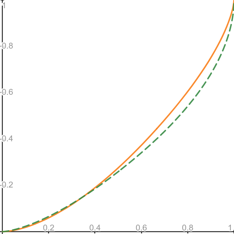
(a) $L_{1}$ (solid) and $L_{2(2)}$ (dashed)

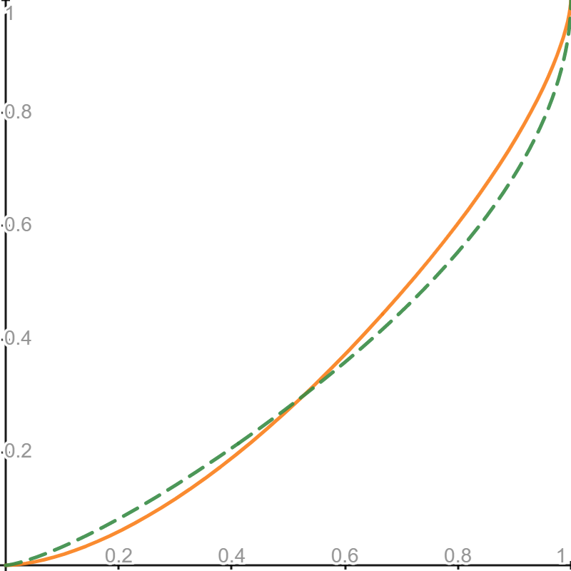
(b) $L_{1}$ (solid) and $L_{2(3)}$ (dashed)

(c) $L_{1}$ (solid) and $L_{2(4)}$ (dashed)

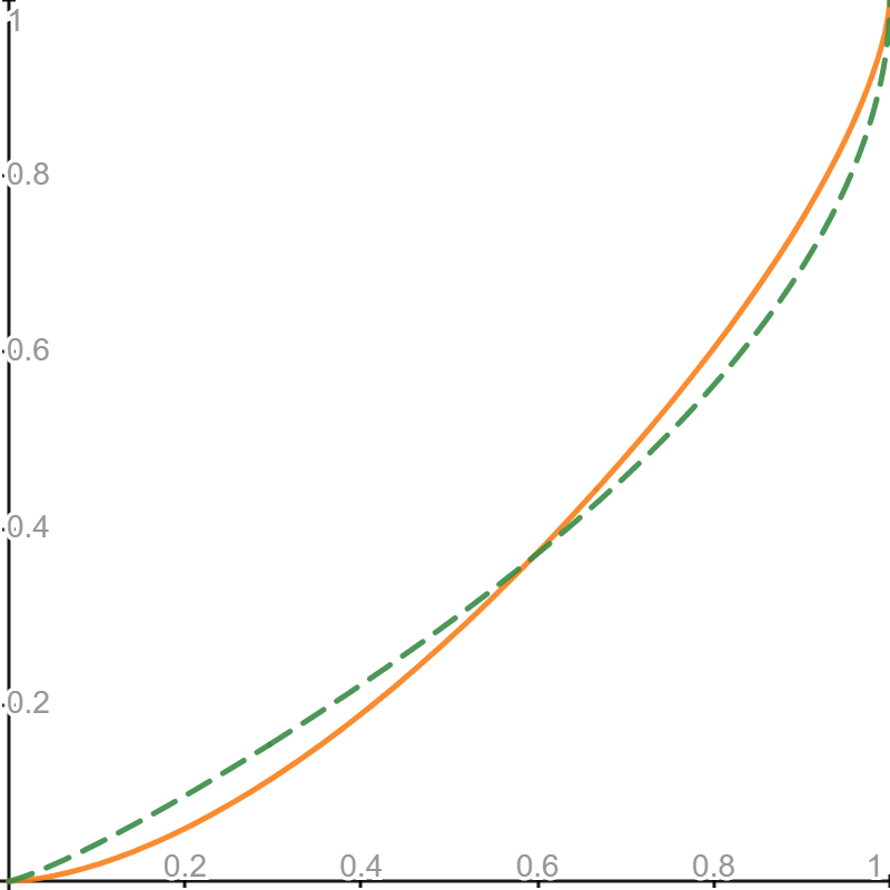
(d) $L_{1}$ (solid) and $L_{2(5)}$ (dashed)

Table 3.1: Estimations and Coverage Rates for LDC (Independent Samples)

DGP	$c(L_{1},L_{2})$	$n_{1}$	$n_{2}$	Mean	Bias	SE	RMSE	$t_{n}$	CR
(a)	0.04703	200	200	0.2305	0.1834	0.3088	0.3592	0.001	0.7040
		200	500	0.1529	0.1058	0.2420	0.2641	0.001	0.7270
		200	1000	0.1258	0.0788	0.2144	0.2284	0.001	0.7200
		1000	2000	0.0733	0.0263	0.0754	0.0798	0.001	0.8630
		10000	10000	0.0523	0.0053	0.0233	0.0239	0.001	0.9330
(b)	0.31489	200	200	0.4753	0.1604	0.3341	0.3706	0.001	0.6970
		200	500	0.3986	0.0837	0.2865	0.2985	0.001	0.7840
		200	1000	0.3695	0.0546	0.2650	0.2706	0.001	0.7900
		1000	2000	0.3515	0.0366	0.1612	0.1653	0.001	0.9140
		10000	10000	0.3260	0.0111	0.0718	0.0727	0.001	0.9330
(c)	0.45198	200	200	0.5680	0.1160	0.3182	0.3387	0.001	0.6720
		200	500	0.5056	0.0537	0.2770	0.2821	0.001	0.7800
		200	1000	0.4811	0.0292	0.2574	0.2590	0.001	0.7940
		1000	2000	0.4804	0.0284	0.1678	0.1702	0.001	0.9100
		10000	10000	0.4619	0.0099	0.0799	0.0805	0.001	0.9260
(d)	0.51960	200	200	0.6114	0.0918	0.3060	0.3195	0.001	0.6690
		200	500	0.5575	0.0379	0.2674	0.2701	0.001	0.7740
		200	1000	0.5360	0.0164	0.2484	0.2489	0.001	0.7850
		1000	2000	0.5427	0.0231	0.1655	0.1671	0.001	0.9030
		10000	10000	0.5283	0.0087	0.0806	0.0811	0.001	0.9280

Table 3.2: Estimations and Coverage Rates for LDC (Matched Pairs)

DGP	$c(L_{1},L_{2})$	$n_{1}$	$n_{2}$	Mean	Bias	SE	RMSE	$t_{n}$	CR
(a)	0.04703	200	200	0.1733	0.1262	0.2616	0.2904	0.001	0.7330
		500	500	0.1173	0.0703	0.1783	0.1917	0.001	0.8280
		1000	1000	0.0914	0.0444	0.1004	0.1097	0.001	0.9010
		2000	2000	0.0692	0.0222	0.0585	0.0626	0.001	0.9070
		10000	10000	0.0491	0.0021	0.0179	0.0181	1.0	0.9380
(b)	0.31489	200	200	0.4158	0.1009	0.3068	0.3230	0.001	0.7560
		500	500	0.4162	0.1013	0.2334	0.2544	0.001	0.8590
		1000	1000	0.3907	0.0758	0.1808	0.1961	0.001	0.9060
		2000	2000	0.3568	0.0419	0.1434	0.1494	0.001	0.9170
		10000	10000	0.3196	0.0047	0.0602	0.0604	7.7	0.9500
(c)	0.45198	200	200	0.5185	0.0665	0.2986	0.3059	0.001	0.7560
		500	500	0.5473	0.0953	0.2249	0.2443	0.001	0.8590
		1000	1000	0.5168	0.0648	0.1811	0.1923	0.001	0.9060
		2000	2000	0.4903	0.0383	0.1546	0.1593	0.001	0.9170
		10000	10000	0.4561	0.0041	0.0686	0.0687	4.4	0.9500
(d)	0.51960	200	200	0.5682	0.0486	0.2898	0.2938	0.001	0.7520
		500	500	0.6094	0.0898	0.2144	0.2325	0.001	0.8510
		1000	1000	0.5752	0.0556	0.1760	0.1845	0.001	0.9000
		2000	2000	0.5547	0.0351	0.1549	0.1589	0.001	0.9060
		10000	10000	0.5232	0.0036	0.0700	0.0701	3.5	0.9500

4 Empirical Application

In this section, we revisit the example of aaberge2021ranking about the inequality growth in the United Kingdom over the past few decades which may be related to the business cycle (blundell2010consumption). We use the replication data of aaberge2021ranking, which originally came from the European Community Household Panel (ECHP) for 1995–2001, and from the European Union Statistics on Income and Living Conditions (EU-SILC) for 2005–2010. In each year, the sample was restricted to households with a male aged 25–64. We follow aaberge2021ranking and focus on the distribution of individual equivalent income adjusted for inflation and differences in household size and composition.

Tables 3 and 4 of aaberge2021ranking report the successful rankings based on the 3rd-degree upward and downward inverse stochastic dominances. They show that the 3rd-degree upward inverse stochastic dominance does not provide a complete ranking for several years. We apply the proposed method to estimate the upward inverse stochastic dominance coefficients (UISDCs) and construct the confidence intervals of these coefficients for some of these years. We compare the latter years ($F_{1}$) with the former years ($F_{2}$) shown in Table 4.1, and find that all the estimated UISDCs are small. Furthermore, the bootstrap confidence intervals are narrow. These facts provide evidence that the income distributions of the latter years may almost upward inverse stochastically dominate the income distributions of the former years, which complements the results of aaberge2021ranking.

Table 4.1: Inequality Growth in the United Kingdom

Year	UISDC	CI	Year	UISDC	CI
94–98	3.2067e-08	[0, 3.0653e-07]	96–98	2.9089e-06	[0, 1.6521e-05]
94–99	1.287e-07	[0, 8.9855e-07]	96–99	5.9121e-06	[0, 3.0879e-05]
94–00	3.0482e-07	[0, 1.7727e-06]	96–00	3.8907e-06	[0, 1.6773e-05]
94–01	3.9715e-07	[0, 2.5549e-06]	96–01	1.2211e-05	[0, 5.0282e-05]
95–98	1.0184e-07	[0, 8.0492e-07]	97–98	0.0063743	[0, 0.056701]
95–99	3.6099e-07	[0, 2.5261e-06]	97–99	0.0091885	[0, 0.069839]
95–00	6.5108e-07	[0, 3.5034e-06]	97–00	8.1315e-05	[0, 0.0004528]
95–01	1.7317e-06	[0, 9.5748e-06]	97–01	0.00027027	[0, 0.0011134]

[sections] [sections]l1

Appendix A Almost Inverse Stochastic Dominance

Following leshno2002preferred, zheng2018almost, and aaberge2021ranking, in this section, we propose almost inverse stochastic dominances, define the inverse stochastic dominance coefficients, and establish an inference procedure for these coefficients. Let $F_{1}$ and $F_{2}$ be two distributions that satisfy Assumption 2.1. Define

$$\Lambda_{j}^{2}\left(p\right)=\int_{0}^{p}F_{j}^{-1}\left(t\right)\mathrm{d}t,\quad p\in\left[0,1\right].$$

Let $P$ denote the social planner’s preference function. As pointed out by yaari1988controversial and aaberge2021ranking, the social welfare functions are consistent with the condition of second-degree stochastic dominance if and only if $P^{\prime}>0$ and $P^{(2)}<0$. We follow aaberge2021ranking and define the set of social planner’s preference functions

$$\mathcal{P}=\left\{\begin{array}[c]{c}P\in C([0,1]):P\left(0\right)=0,P\left(1\right)=1,P^{\prime}\left(1\right)=0,\\ P^{\prime}\left(t\right)>0\text{ and }P^{\left(2\right)}\left(t\right)<0\text{ for all }t\in\left(0,1\right)\end{array}\right\}.$$

We then define the welfare functions $W_{P}$ such that for every $P\in\mathcal{P}$ and every CDF $F$,

$$W_{P}\left(F\right)=\int_{0}^{1}P^{\prime}\left(t\right)F^{-1}\left(t\right)\mathrm{d}t.$$

Theorem 1 of aaberge2001axiomatic demonstrates that a person who supports Axioms 1–4 in aaberge2001axiomatic ranks Lorenz curves according to the criterion $W_{P}$.

Remark A.1

aaberge2021ranking discuss the relationship between the inequality measure $J_{P}$ defined in (2.10) and the social welfare measure $W_{P}$. ebert1987size shows that for every preference function $P\in\mathcal{P}$ and every distribution function $F$ that satisfies Assumption 2.1, $W_{P}(F)=\mu_{F}(1-J_{P}(L_{F}))$, where $\mu_{F}$ denotes the population mean for $F$ and $L_{F}$ denotes the Lorenz curve corresponding to $F$. As pointed out by aaberge2021ranking, the product $\mu_{F}J_{P}(L_{F})$ presents the loss in social welfare due to inequality in the distribution.

A.1 Almost Upward Inverse Stochastic Dominance and Social Welfare

For $m\geq 3$, define

$$\Lambda_{j}^{m}\left(p\right) =\int_{0}^{p}\Lambda_{j}^{m-1}\left(t\right)\mathrm{d}t=\int_{0}^{p}\cdots\int_{0}^{t_{3}}\int_{0}^{t_{2}}F_{j}^{-1}\left(t_{1}\right)\mathrm{d}t_{1}\mathrm{d}t_{2}\cdots\mathrm{d}t_{m-1}$$

$$=\frac{1}{\left(m-2\right)!}\int_{0}^{p}\left(p-t\right)^{m-2}F^{-1}\left(t\right)\mathrm{d}t,\quad p\in\left[0,1\right].$$

aaberge2021ranking introduce the $m$th-degree upward inverse stochastic dominance for $m\geq 3$.

Definition A.1

A distribution $F_{1}$ $m$th-degree upward inverse stochastically dominates a distribution $F_{2}$ if $\Lambda_{1}^{m}\left(p\right)\geq\Lambda_{2}^{m}\left(p\right)$ for all $p\in\left[0,1\right]$.

When $m=2$, the upward inverse stochastic dominance is the generalized Lorenz dominance. We generalize the upward inverse stochastic dominance in aaberge2021ranking to almost upward inverse stochastic dominance.

Definition A.2

For every $\varepsilon_{m}\in[0,1/2)$, the CDF $F_{1}$ $\varepsilon_{m}$-almost $m$th-degree upward inverse stochastically dominates the CDF $F_{2}$ ($F_{1}$ $\varepsilon_{m}$-A$m$UISD $F_{2}$), if

$$\int_{0}^{1}\max\left(\Lambda_{2}^{m}\left(p\right)-\Lambda_{1}^{m}\left(p\right),0\right)\mathrm{d}p\leq\varepsilon_{m}\int_{0}^{1}\left|\Lambda_{2}^{m}\left(p\right)-\Lambda_{1}^{m}\left(p\right)\right|\mathrm{d}p.$$ (A.1)

For every $\varepsilon_{m}\in\left(0,1/2\right)$, we define

$$\mathcal{P}_{m}\left(\varepsilon_{m}\right)=\left\{\begin{array}[c]{c}P\in\mathcal{P}:\left(-1\right)^{m-1}P^{\left(m\right)}\geq 0,P^{\left(j\right)}\left(1\right)=0\text{ for }j\in\{2,\ldots,m-1\},\\ \sup_{t}\left\{\left(-1\right)^{m-1}P^{\left(m\right)}\left(t\right)\right\}\leq\inf_{t}\left\{\left(-1\right)^{m-1}P^{\left(m\right)}\left(t\right)\right\}\cdot\left(\frac{1}{\varepsilon_{m}}-1\right)\end{array}\right\}$$

and

$$\mathcal{P}_{m}^{\prime}\left(\varepsilon_{m}\right)=\left\{\begin{array}[c]{c}P\in\mathcal{P}:\left(-1\right)^{m-1}P^{\left(m\right)}\geq 0,\left(-1\right)^{j-1}P^{\left(j\right)}\left(1\right)\geq 0\text{ for }j\in\{2,\ldots,m-1\},\\ \sup_{t}\left\{\left(-1\right)^{m-1}P^{\left(m\right)}\left(t\right)\right\}\leq\inf_{t}\left\{\left(-1\right)^{m-1}P^{\left(m\right)}\left(t\right)\right\}\cdot\left(\frac{1}{\varepsilon_{m}}-1\right)\end{array}\right\}.$$

Then the following proposition links A$m$UISD to the social welfare function $W_{P}$ with $P$ from $\mathcal{P}_{m}(\varepsilon_{m})$ and $\mathcal{P}^{\prime}_{m}(\varepsilon_{m})$.

Proposition A.1

For every $\varepsilon_{m}\in\left(0,1/2\right)$, if $F_{1}$ $\varepsilon_{m}$-A$m$UISD $F_{2}$, then $W_{P}\left(F_{1}\right)\geq W_{P}\left(F_{2}\right)$ for every $P\in\mathcal{P}_{m}\left(\varepsilon_{m}\right)$. If $F_{1}$ $\varepsilon_{m}$-A$m$UISD $F_{2}$ and $\Lambda_{1}^{j}\left(1\right)\geq\Lambda_{2}^{j}\left(1\right)$ for all $j\in\left\{3,\ldots,m\right\}$, then $W_{P}\left(F_{1}\right)\geq W_{P}\left(F_{2}\right)$ for every $P\in\mathcal{P}_{m}^{\prime}\left(\varepsilon_{m}\right)$.

For $m\geq 3$, following Lemma 2.1, it is straightforward to show that $F_{1}$ $\varepsilon_{m}$-A$m$UISD $F_{2}$ if and only if there is $c_{m}\in\left[0,\varepsilon_{m}\right]$ such that

$$\int_{0}^{1}\max\left(\Lambda_{2}^{m}\left(p\right)-\Lambda_{1}^{m}\left(p\right),0\right)\mathrm{d}p=c_{m}\int_{0}^{1}\left|\Lambda_{2}^{m}\left(p\right)-\Lambda_{1}^{m}\left(p\right)\right|\mathrm{d}p.$$

We now define the upward inverse stochastic dominance coefficient as follows.

Definition A.3

For $m\geq 3$, the $F_{1}$-$F_{2}$ $m$th-degree upward inverse stochastic dominance coefficient ($F_{1}$-$F_{2}$ $m$UISDC), denoted by $c_{m}^{u}(F_{1},F_{2})$, is defined as

$$c_{m}^{u}(F_{1},F_{2})=$$

$$\inf\left\{\varepsilon_{m}\in[0,1]:\int_{0}^{1}\max\left(\Lambda_{2}^{m}\left(p\right)-\Lambda_{1}^{m}\left(p\right),0\right)\mathrm{d}p\leq\varepsilon_{m}\int_{0}^{1}\left|\Lambda_{2}^{m}\left(p\right)-\Lambda_{1}^{m}\left(p\right)\right|\mathrm{d}p\right\}.$$ (A.2)

We define the difference function

$$\phi_{m}^{u}\left(p\right)=\Lambda_{2}^{m}\left(p\right)-\Lambda_{1}^{m}\left(p\right),\quad p\in[0,1].$$ (A.3)

The following lemma summarizes the properties of the $m$UISDC $c_{m}^{u}(F_{1},F_{2})$.

Lemma A.1

The $m$UISDC $c_{m}^{u}(F_{1},F_{2})$ is the smallest $\varepsilon_{m}$ in $[0,1]$ such that (A.1) holds. With (1.1), it follows that

$$c_{m}^{u}(F_{1},F_{2}) =\frac{\int_{0}^{1}\max\left(\Lambda_{2}^{m}\left(p\right)-\Lambda_{1}^{m}\left(p\right),0\right)\mathrm{d}p}{\int_{0}^{1}\left|\Lambda_{1}^{m}\left(p\right)-\Lambda_{2}^{m}\left(p\right)\right|\mathrm{d}p}$$

$$=\frac{\int_{0}^{1}\max\left\{\phi_{m}^{u}\left(p\right),0\right\}\mathrm{d}p}{\int_{0}^{1}\max\left\{\phi_{m}^{u}\left(p\right),0\right\}\mathrm{d}p+\int_{0}^{1}\max\left\{-\phi_{m}^{u}\left(p\right),0\right\}\mathrm{d}p}.$$ (A.4)

In addition, if $c_{m}^{u}(F_{1},F_{2})\in(0,1]$, then $c_{m}^{u}(F_{2},F_{1})=1-c_{m}^{u}(F_{1},F_{2})$.

According to Lemma A.1, $F_{1}$ $\varepsilon_{m}$-A$m$UISD $F_{2}$ for all $\varepsilon_{m}\in[c_{m}^{u}(F_{1},F_{2}),1/2)$ if $c_{m}^{u}(F_{1},F_{2})<1/2$. On the other hand, $c_{m}^{u}(F_{1},F_{2})>1/2$ implies that $F_{2}$ $\varepsilon_{m}$-A$m$UISD $F_{1}$ for all $\varepsilon_{m}\in[1-c_{m}^{u}(F_{1},F_{2}),1/2)$. Thus, $c_{m}^{u}(F_{1},F_{2})$ presents the degree of almost upward inverse stochastic dominance relationship between $F_{1}$ and $F_{2}$, and provides all $\varepsilon_{m}$ such that the $\varepsilon_{m}$-A$m$UISD holds.

Proposition A.2

If $c_{m}^{u}(F_{1},F_{2})\in(0,1/2)$, it then follows that $W_{P}(F_{1})\geq W_{P}(F_{2})\text{ for all }P\in\cup_{\varepsilon_{m}\in[c_{m}^{u}(F_{1},F_{2}),1/2)}\mathcal{P}_{m}(\varepsilon_{m})$. If, in addition, $\Lambda_{1}^{j}\left(1\right)\geq\Lambda_{2}^{j}\left(1\right)$ for all $j\in\left\{3,\ldots,m\right\}$, it follows that $W_{P}\left(F_{1}\right)\geq W_{P}\left(F_{2}\right)$ for every $P\in\cup_{\varepsilon_{m}\in[c_{m}^{u}(F_{1},F_{2}),1/2)}\mathcal{P}_{m}^{\prime}\left(\varepsilon_{m}\right)$.

Similar to Proposition 2.1, Proposition A.2 shows the importance of UISDC concerning welfare functions $W_{P}$. The smaller the UISDC $c_{m}^{u}(F_{1},F_{2})$ is, the more welfare functions show higher welfare for the distribution $F_{1}$ compared to $F_{2}$. With the knowledge of $c_{m}^{u}(F_{1},F_{2})$, we can infer the relationship between $F_{1}$ and $F_{2}$ based on a class of welfare functions.

A.2 Almost Downward Inverse Stochastic Dominance and Social Welfare

aaberge2021ranking introduce the $m$th-degree downward inverse stochastic dominance for $m\geq 3$. For $j=1,2$, define

$$\tilde{\Lambda}_{j}^{3}\left(p\right) =\int_{p}^{1}\Lambda_{j}^{2}\left(t\right)\mathrm{d}t=\int_{0}^{1}\Lambda_{j}^{2}\left(t\right)\mathrm{d}t-\Lambda_{j}^{3}\left(p\right)$$

$$=\left(1-p\right)\int_{0}^{1}F_{j}^{-1}\left(t\right)\mathrm{d}t-\int_{p}^{1}\left(t-p\right)F_{j}^{-1}\left(t\right)\mathrm{d}t,\quad p\in\left[0,1\right].$$

For $m\geq 4$, define

$$\tilde{\Lambda}_{j}^{m}\left(p\right) =\int_{p}^{1}\tilde{\Lambda}_{j}^{m-1}\left(t\right)\mathrm{d}t=\int_{p}^{1}\cdots\int_{t_{3}}^{1}\int_{0}^{t_{2}}F_{j}^{-1}\left(t_{1}\right)\mathrm{d}t_{1}\mathrm{d}t_{2}\cdots\mathrm{d}t_{m-1}$$

$$=\frac{1}{\left(m-2\right)!}\left[\left(1-p\right)^{m-2}\int_{0}^{1}F^{-1}\left(t\right)\mathrm{d}t-\int_{p}^{1}\left(t-p\right)^{m-2}F^{-1}\left(t\right)\mathrm{d}t\right],\quad p\in\left[0,1\right].$$

Definition A.4

A distribution $F_{1}$ $m$th-degree downward inverse stochastically dominates a distribution $F_{2}$ if $\tilde{\Lambda}_{1}^{m}\left(p\right)\geq\tilde{\Lambda}_{2}^{m}\left(p\right)$ for all $p\in\left[0,1\right]$.

We generalize the downward inverse stochastic dominance in aaberge2021ranking to almost downward inverse stochastic dominance.

Definition A.5

For every $\varepsilon_{m}\in[0,1/2)$, the CDF $F_{1}$ $\varepsilon_{m}$-almost $m$th-degree downward inverse stochastically dominates the CDF $F_{2}$ ($F_{1}$ $\varepsilon_{m}$-A$m$DISD $F_{2}$), if

$$\int_{0}^{1}\max\left(\tilde{\Lambda}_{2}^{m}\left(p\right)-\tilde{\Lambda}_{1}^{m}\left(p\right),0\right)\mathrm{d}p\leq\varepsilon_{m}\int_{0}^{1}\left|\tilde{\Lambda}_{2}^{m}\left(p\right)-\tilde{\Lambda}_{1}^{m}\left(p\right)\right|\mathrm{d}p.$$

For every $\varepsilon_{m}\in\left(0,1/2\right)$, we define

$$\mathcal{\tilde{P}}_{m}\left(\varepsilon_{m}\right)=\left\{\begin{array}[c]{c}P\in\mathcal{P}:P^{\left(m\right)}\leq 0,P^{\left(j\right)}\left(0\right)=0\text{ for }j\in\{2,\ldots,m-1\},\\ \sup_{t}\left\{-P^{\left(m\right)}\left(t\right)\right\}\leq\inf_{t}\left\{-P^{\left(m\right)}\left(t\right)\right\}\cdot\left(\frac{1}{\varepsilon_{m}}-1\right)\end{array}\right\}$$

and

$$\mathcal{\tilde{P}}_{m}^{\prime}\left(\varepsilon_{m}\right)=\left\{\begin{array}[c]{c}P\in\mathcal{P}:P^{\left(m\right)}\leq 0,P^{\left(j\right)}\left(0\right)\leq 0\text{ for }j\in\{2,\ldots,m-1\},\\ \sup_{t}\left\{-P^{\left(m\right)}\left(t\right)\right\}\leq\inf_{t}\left\{-P^{\left(m\right)}\left(t\right)\right\}\cdot\left(\frac{1}{\varepsilon_{m}}-1\right)\end{array}\right\}.$$

Then the following proposition links A$m$DISD to the social welfare function $W_{P}$ with $P$ from $\tilde{\mathcal{P}}_{m}(\varepsilon_{m})$ and $\tilde{\mathcal{P}}^{\prime}_{m}(\varepsilon_{m})$.

Proposition A.3

For every $\varepsilon_{m}\in\left(0,1/2\right)$, if $F_{1}$ $\varepsilon_{m}$-A$m$DISD $F_{2}$, then $W_{P}\left(F_{1}\right)\geq W_{P}\left(F_{2}\right)$ for every $P\in\mathcal{\tilde{P}}_{m}\left(\varepsilon_{m}\right)$. If $F_{1}$ $\varepsilon_{m}$-A$m$DISD $F_{2}$ and $\tilde{\Lambda}_{1}^{j}\left(0\right)\geq\tilde{\Lambda}_{2}^{j}\left(0\right)$ for all $j\in\left\{3,\ldots,m\right\}$, then $W_{P}\left(F_{1}\right)\geq W_{P}\left(F_{2}\right)$ for every $P\in\mathcal{\tilde{P}}_{m}^{\prime}\left(\varepsilon_{m}\right)$.

For $m\geq 3$, following Lemma 2.1, it is straightforward to show that $F_{1}$ $\varepsilon_{m}$-A$m$DISD $F_{2}$ if and only if there is $c_{m}\in\left[0,\varepsilon_{m}\right]$ such that

$$\int_{0}^{1}\max\left(\tilde{\Lambda}_{2}^{m}\left(p\right)-\tilde{\Lambda}_{1}^{m}\left(p\right),0\right)\mathrm{d}p=c_{m}\int_{0}^{1}\left|\tilde{\Lambda}_{2}^{m}\left(p\right)-\tilde{\Lambda}_{1}^{m}\left(p\right)\right|\mathrm{d}p.$$

We now define the downward inverse stochastic dominance coefficient as follows.

Definition A.6

For $m\geq 3$, the $F_{1}$-$F_{2}$ $m$th-degree downward inverse stochastic dominance coefficient ($F_{1}$-$F_{2}$ $m$DISDC), denoted by $c_{m}^{d}(F_{1},F_{2})$, is defined as

$$c_{m}^{d}(F_{1},F_{2})=$$

$$\inf\left\{\varepsilon_{m}\in[0,1]:\int_{0}^{1}\max\left(\tilde{\Lambda}_{2}^{m}\left(p\right)-\tilde{\Lambda}_{1}^{m}\left(p\right),0\right)\mathrm{d}p\leq\varepsilon_{m}\int_{0}^{1}\left|\tilde{\Lambda}_{2}^{m}\left(p\right)-\tilde{\Lambda}_{1}^{m}\left(p\right)\right|\mathrm{d}p\right\}.$$ (A.5)

We define the difference function

$$\phi_{m}^{d}\left(p\right)=\tilde{\Lambda}_{2}^{m}\left(p\right)-\tilde{\Lambda}_{1}^{m}\left(p\right),\quad p\in[0,1].$$ (A.6)

The following lemma summarizes the properties of the $m$DISDC $c_{m}^{d}(F_{1},F_{2})$.

Lemma A.2

The $m$DISDC $c_{m}^{d}(F_{1},F_{2})$ is the smallest $\varepsilon_{m}$ in $[0,1]$ such that (A.6) holds. With (1.1), it follows that

$$c_{m}^{d}(F_{1},F_{2}) =\frac{\int_{0}^{1}\max\left(\tilde{\Lambda}_{2}^{m}\left(p\right)-\tilde{\Lambda}_{1}^{m}\left(p\right),0\right)\mathrm{d}p}{\int_{0}^{1}\left|\tilde{\Lambda}_{1}^{m}\left(p\right)-\tilde{\Lambda}_{2}^{m}\left(p\right)\right|\mathrm{d}p}$$

$$=\frac{\int_{0}^{1}\max\left\{\phi_{m}^{d}\left(p\right),0\right\}\mathrm{d}p}{\int_{0}^{1}\max\left\{\phi_{m}^{d}\left(p\right),0\right\}\mathrm{d}p+\int_{0}^{1}\max\left\{-\phi_{m}^{d}\left(p\right),0\right\}\mathrm{d}p}.$$ (A.7)

In addition, if $c_{m}^{d}(F_{1},F_{2})\in(0,1]$, then $c_{m}^{d}(F_{2},F_{1})=1-c_{m}^{d}(F_{1},F_{2})$.

According to Lemma A.2, $F_{1}$ $\varepsilon_{m}$-A$m$DISD $F_{2}$ for all $\varepsilon_{m}\in[c_{m}^{d}(F_{1},F_{2}),1/2)$ if $c_{m}^{d}(F_{1},F_{2})<1/2$. On the other hand, $c_{m}^{d}(F_{1},F_{2})>1/2$ implies that $F_{2}$ $\varepsilon_{m}$-A$m$DISD $F_{1}$ for all $\varepsilon_{m}\in[1-c_{m}^{d}(F_{1},F_{2}),1/2)$. Thus, $c_{m}^{d}(F_{1},F_{2})$ presents the degree of almost downward inverse stochastic dominance relationship between $F_{1}$ and $F_{2}$, and provides all $\varepsilon_{m}$ such that the $\varepsilon_{m}$-A$m$DISD holds.

Proposition A.4

If $c_{m}^{d}(F_{1},F_{2})\in(0,1/2)$, it then follows that $W_{P}(F_{1})\geq W_{P}(F_{2})$ for all $P\in\cup_{\varepsilon_{m}\in[c_{m}^{d}(F_{1},F_{2}),1/2)}\tilde{\mathcal{P}}_{m}(\varepsilon_{m})$. If, in addition, $\tilde{\Lambda}_{1}^{j}\left(0\right)\geq\tilde{\Lambda}_{2}^{j}\left(0\right)$ for all $j\in\left\{3,\ldots,m\right\}$, then $W_{P}\left(F_{1}\right)\geq W_{P}\left(F_{2}\right)$ for every $P\in\cup_{\varepsilon_{m}\in[c_{m}^{d}(F_{1},F_{2}),1/2)}\mathcal{\tilde{P}}_{m}^{\prime}\left(\varepsilon_{m}\right)$.

Similar to Proposition 2.1, Proposition A.4 shows the importance of DISDC concerning welfare functions $W_{P}$. The smaller the DISDC $c_{m}^{d}(F_{1},F_{2})$ is, the more welfare functions show higher welfare for the distribution $F_{1}$ compared to $F_{2}$. With the knowledge of $c_{m}^{d}(F_{1},F_{2})$, we can infer the relationship between $F_{1}$ and $F_{2}$ based on a class of welfare functions.

A.3 Estimation and Inference

Let $\mathcal{F}$, $\hat{F}_{j}$, and $\hat{Q}_{j}$ be defined as in (2.3.2), (2.19), and (2.20). Let $\mathcal{B}_{1}$ and $\mathcal{B}_{2}$ be the centered Gaussian random elements in $C(\left[0,1\right])$ defined in Section 2.3.3. It is straightforward to show that (see the proof of Lemma B.2)

$$\left(\begin{array}[c]{c}n_{1}^{1/2}\left(\hat{F}_{1}-F_{1}\right)\\ n_{2}^{1/2}\left(\hat{F}_{2}-F_{2}\right)\end{array}\right)\leadsto\left(\begin{array}[c]{c}\mathcal{B}_{1}\circ F_{1}\\ \mathcal{B}_{2}\circ F_{2}\end{array}\right)$$

in $\ell^{\infty}\left([0,\infty)\right)\times\ell^{\infty}\left([0,\infty)\right)$. Beare2017improved show that under Assumptions 2.1 and 2.2, we can apply the results of K17 and obtain

$$\left(\begin{array}[c]{c}n_{1}^{1/2}\left(\hat{Q}_{1}-Q_{1}\right)\\ n_{2}^{1/2}\left(\hat{Q}_{2}-Q_{2}\right)\end{array}\right)\leadsto\left(\begin{array}[c]{c}-Q_{1}^{\prime}\cdot\mathcal{B}_{1}\\ -Q_{2}^{\prime}\cdot\mathcal{B}_{2}\end{array}\right)$$

in $L^{1}\left([0,1]\right)\times L^{1}\left([0,1]\right)$. Recall that for all $p\in\left[0,1\right]$, $\Lambda_{j}^{2}\left(p\right)=\int_{0}^{p}Q_{j}\left(t\right)\mathrm{d}t$ and we estimate $\Lambda_{j}^{2}\left(p\right)$ by $\hat{\Lambda}_{j}^{2}\left(p\right)=\int_{0}^{p}\hat{Q}_{j}\left(t\right)\mathrm{d}t$. As shown in jiang2023nonparametric, by continuous mapping theorem,

$$\left(\begin{array}[c]{c}n_{1}^{1/2}\left(\hat{\Lambda}_{1}^{2}-{\Lambda}_{1}^{2}\right)\\ n_{2}^{1/2}\left(\hat{\Lambda}_{2}^{2}-{\Lambda}_{2}^{2}\right)\end{array}\right)\leadsto\binom{\mathcal{V}_{1}}{\mathcal{V}_{2}},$$ (A.10)

where $\mathcal{V}_{j}=\int_{0}^{p}-Q_{j}^{\prime}\left(t\right)\mathcal{B}_{j}(t)\mathrm{d}t$. By continuous mapping theorem again, it follows that

$$\sqrt{T_{n}}\left\{(\hat{\Lambda}_{2}^{2}-\hat{\Lambda}_{1}^{2})-\left(\Lambda_{2}^{2}-\Lambda_{1}^{2}\right)\right\}\leadsto\mathbb{G}_{\Lambda},$$

where $\mathbb{G}_{\Lambda}=\sqrt{\lambda}\mathcal{V}_{2}-\sqrt{1-\lambda}\mathcal{V}_{1}$ and for all $p,p^{\prime}\in\left[0,1\right]$,

$$E\left[\mathbb{G}_{\Lambda}\left(p\right)\mathbb{G}_{\Lambda}\left(p^{\prime}\right)\right]= \,\left(1-\lambda\right)E\left[\mathcal{V}_{1}\left(p\right)\mathcal{V}_{1}\left(p^{\prime}\right)\right]-\sqrt{\lambda\left(1-\lambda\right)}E\left[\mathcal{V}_{1}\left(p\right)\mathcal{V}_{2}\left(p^{\prime}\right)\right]$$

$$-\sqrt{\lambda\left(1-\lambda\right)}E\left[\mathcal{V}_{2}\left(p\right)\mathcal{V}_{1}\left(p^{\prime}\right)\right]+\lambda E\left[\mathcal{V}_{2}\left(p\right)\mathcal{V}_{2}\left(p^{\prime}\right)\right].$$

By Lemma 3.1 of jiang2023nonparametric, for $j,j^{\prime}\in\left\{1,2\right\}$ and $p,p^{\prime}\in\left[0,1\right]$, we have that

$$E\left[\mathcal{V}_{j}\left(p\right)\mathcal{V}_{j^{\prime}}(p^{\prime})\right]=Cov\left(Q_{j}\left(p\right)\wedge X_{i}^{j},Q_{j^{\prime}}(p^{\prime})\wedge X_{i}^{j^{\prime}}\right).$$ (A.11)

For $j=1,2$, $m\geq 3$, and $p\in[0,1]$, define

$$\hat{\Lambda}_{j}^{m}\left(p\right)=\int_{0}^{p}\cdots\int_{0}^{t_{3}}\int_{0}^{t_{2}}\hat{Q}_{j}\left(t_{1}\right)\mathrm{d}t_{1}\mathrm{d}t_{2}\cdots\mathrm{d}t_{m-1}=\int_{0}^{p}\cdots\int_{0}^{t_{3}}\hat{\Lambda}_{j}^{2}\left(t_{2}\right)\mathrm{d}t_{2}\cdots\mathrm{d}t_{m-1}$$

and

$$\hat{\tilde{\Lambda}}_{j}^{m}\left(p\right)=\int_{p}^{1}\cdots\int_{t_{3}}^{1}\int_{0}^{t_{2}}\hat{Q}_{j}\left(t_{1}\right)\mathrm{d}t_{1}\mathrm{d}t_{2}\cdots\mathrm{d}t_{m-1}=\int_{p}^{1}\cdots\int_{t_{3}}^{1}\hat{\Lambda}_{j}^{2}\left(t_{2}\right)\mathrm{d}t_{2}\cdots\mathrm{d}t_{m-1}.$$

For $m\geq 3$, define the empirical difference functions

$$\hat{\phi}_{m}^{u}\left(p\right)=\hat{\Lambda}_{2}^{m}\left(p\right)-\hat{\Lambda}_{1}^{m}\left(p\right)\text{ and }{\hat{\phi}}_{m}^{d}\left(p\right)=\hat{\tilde{\Lambda}}_{2}^{m}\left(p\right)-\hat{\tilde{\Lambda}}_{1}^{m}\left(p\right),\quad p\in[0,1].$$

The estimator for $c_{m}^{w}\left(F_{1},F_{2}\right)$ can be constructed by

$$\hat{c}_{m}^{w}\left(F_{1},F_{2}\right)=\frac{\mathcal{F}_{1}(\hat{\phi}_{m}^{w})}{\mathcal{F}_{1}(\hat{\phi}_{m}^{w})+\mathcal{F}_{2}(\hat{\phi}_{m}^{w})}=\mathcal{F}(\hat{\phi}_{m}^{w}).$$

Similar to Proposition 2.6, we can show that $\mathcal{F}$ is Hadamard directionally differentiable at $\phi_{m}^{w}$ defined in (A.3) and (A.6) such that for every $h\in\ell^{\infty}([0,1])$,

$$\mathcal{F}_{\phi_{m}^{w}}^{\prime}\left(h\right)=\frac{\mathcal{F}_{1\phi_{m}^{w}}^{\prime}\left(h\right)\mathcal{F}_{2}\left(\phi_{m}^{w}\right)-\mathcal{F}_{1}\left(\phi_{m}^{w}\right)\mathcal{F}_{2\phi_{m}^{w}}^{\prime}\left(h\right)}{\left(\mathcal{F}_{1}\left(\phi_{m}^{w}\right)+\mathcal{F}_{2}\left(\phi_{m}^{w}\right)\right)^{2}},$$

where

$$\mathcal{F}_{1\phi_{m}^{w}}^{\prime}\left(h\right)=\int_{B_{+}\left(\phi_{m}^{w}\right)}h\left(p\right)\mathrm{d}p+\int_{B_{0}\left(\phi_{m}^{w}\right)}\max\left\{h\left(p\right),0\right\}\mathrm{d}p$$

and

$$\mathcal{F}_{2\phi_{m}^{w}}^{\prime}\left(h\right)=\int_{B_{+}\left(-\phi_{m}^{w}\right)}-h\left(p\right)\mathrm{d}p+\int_{B_{0}\left(\phi_{m}^{w}\right)}\max\left\{-h\left(p\right),0\right\}\mathrm{d}p$$

with $B_{0}$ and $B_{+}$ defined in (2.23).

Proposition A.5

Under Assumptions 2.1 and 2.2, for $m\geq 3$ and $w\in\{u,d\}$, it follows that

$$\sqrt{T_{n}}(\hat{\phi}_{m}^{w}-\phi_{m}^{w})\leadsto\mathbb{G}_{m}^{w}$$

for some random element $\mathbb{G}_{m}^{w}$ with

$$Var(\mathbb{G}_{m}^{u}(p))=\int_{0}^{p}\cdots\int_{0}^{t_{3}^{\prime}}\left(\int_{0}^{p}\cdots\int_{0}^{t_{3}}E\left[\mathbb{G}_{\Lambda}(t_{2})\mathbb{G}_{\Lambda}(t_{2}^{\prime})\right]\mathrm{d}t_{2}\cdots\mathrm{d}t_{m-1}\right)\mathrm{d}t_{2}^{\prime}\cdots\mathrm{d}t_{m-1}^{\prime}$$

and

$$Var(\mathbb{G}_{m}^{d}(p))=\int_{p}^{1}\cdots\int_{t_{3}^{\prime}}^{1}\left(\int_{p}^{1}\cdots\int_{t_{3}}^{1}E\left[\mathbb{G}_{\Lambda}(t_{2})\mathbb{G}_{\Lambda}(t_{2}^{\prime})\right]\mathrm{d}t_{2}\cdots\mathrm{d}t_{m-1}\right)\mathrm{d}t_{2}^{\prime}\cdots\mathrm{d}t_{m-1}^{\prime}$$

for every $p\in[0,1]$. Moreover, we have that

$$\sqrt{T_{n}}\left\{\hat{c}_{m}^{w}\left(F_{1},F_{2}\right)-c_{m}^{w}\left(F_{1},F_{2}\right)\right\}\leadsto\mathcal{F}_{\phi_{m}^{w}}^{\prime}\left(\mathbb{G}_{m}^{w}\right).$$

Let $\hat{\lambda}=n_{1}/(n_{1}+n_{2})$. For $j,j^{\prime}\in\left\{1,2\right\}$ and $p,p^{\prime}\in\left[0,1\right]$, by (A.11), we estimate $E\left[\mathcal{V}_{j}\left(p\right)\mathcal{V}_{j^{\prime}}\left(p^{\prime}\right)\right]$ by $\hat{E}\left[\mathcal{V}_{j}\left(p\right)\mathcal{V}_{j^{\prime}}\left(p^{\prime}\right)\right]$ which is defined as the sample covariance of the two samples

$$\left\{\hat{Q}_{j}(p)\wedge X^{j}_{i}\right\}_{i=1}^{n_{j}}\text{ and }\left\{\hat{Q}_{j^{\prime}}(p^{\prime})\wedge X^{j^{\prime}}_{i}\right\}_{i=1}^{n_{j^{\prime}}}.$$

For independent samples, we estimate $E\left[\mathbb{G}_{\Lambda}\left(p\right)\mathbb{G}_{\Lambda}\left(p^{\prime}\right)\right]$ by

$$\hat{E}\left[\mathbb{G}_{\Lambda}\left(p\right)\mathbb{G}_{\Lambda}(p^{\prime})\right]=(1-\hat{\lambda})\hat{E}\left[\mathcal{V}_{1}\left(p\right)\mathcal{V}_{1}(p^{\prime})\right]+\hat{\lambda}\hat{E}\left[\mathcal{V}_{2}\left(p\right)\mathcal{V}_{2}(p^{\prime})\right].$$

For matched pairs,

$$\hat{E}\left[\mathbb{G}_{\Lambda}\left(p\right)\mathbb{G}_{\Lambda}(p^{\prime})\right]= \,(1-\hat{\lambda})\hat{E}\left[\mathcal{V}_{1}\left(p\right)\mathcal{V}_{1}(p^{\prime})\right]-\sqrt{\hat{\lambda}(1-\hat{\lambda})}\hat{E}\left[\mathcal{V}_{1}\left(p\right)\mathcal{V}_{2}(p^{\prime})\right]$$

$$-\sqrt{\hat{\lambda}(1-\hat{\lambda})}\hat{E}\left[\mathcal{V}_{2}\left(p\right)\mathcal{V}_{1}(p^{\prime})\right]+\hat{\lambda}\hat{E}\left[\mathcal{V}_{2}\left(p\right)\mathcal{V}_{2}(p^{\prime})\right].$$

We then estimate the variance $Var(\mathbb{G}_{m}^{w}(p))$ by

$$\hat{\sigma}_{m}^{u}(p)^{2}=\int_{0}^{p}\cdots\int_{0}^{t_{3}^{\prime}}\left(\int_{0}^{p}\cdots\int_{0}^{t_{3}}\hat{E}\left[\mathbb{G}_{\Lambda}(t_{2})\mathbb{G}_{\Lambda}(t_{2}^{\prime})\right]\mathrm{d}t_{2}\cdots\mathrm{d}t_{m-1}\right)\mathrm{d}t_{2}^{\prime}\cdots\mathrm{d}t_{m-1}^{\prime}$$

and

$$\hat{\sigma}_{m}^{d}(p)^{2}=\int_{p}^{1}\cdots\int_{t_{3}^{\prime}}^{1}\left(\int_{p}^{1}\cdots\int_{t_{3}}^{1}\hat{E}\left[\mathbb{G}_{\Lambda}(t_{2})\mathbb{G}_{\Lambda}(t_{2}^{\prime})\right]\mathrm{d}t_{2}\cdots\mathrm{d}t_{m-1}\right)\mathrm{d}t_{2}^{\prime}\cdots\mathrm{d}t_{m-1}^{\prime}$$

for $p\in[0,1]$.

A.3.1 Bootstrap Confidence Intervals for UISDC and DISDC

Similar to Section 2.3.4, for $m\geq 3$ and $w\in\{u,d\}$, we construct the estimators of $B_{+}\left(\phi_{m}^{w}\right)$, $B_{+}\left(-\phi_{m}^{w}\right)$, and $B_{0}\left(\phi_{m}^{w}\right)$ by

$$\widehat{B_{+}\left(\phi^{w}_{m}\right)}=\left\{p\in\left[0,1\right]:\frac{\sqrt{T_{n}}\hat{\phi}^{w}_{m}\left(p\right)}{\xi_{0}\vee\hat{\sigma}^{w}_{m}\left(p\right)}>t_{n}\right\},\widehat{B_{+}\left(-\phi^{w}_{m}\right)}=\left\{p\in\left[0,1\right]:\frac{\sqrt{T_{n}}\hat{\phi}^{w}_{m}\left(p\right)}{\xi_{0}\vee\hat{\sigma}^{w}_{m}\left(p\right)}<-t_{n}\right\},$$

$$\text{and }\widehat{B_{0}\left(\phi_{m}^{w}\right)}=\left\{p\in\left[0,1\right]:\left|\frac{\sqrt{T_{n}}\hat{\phi}^{w}_{m}\left(p\right)}{\xi_{0}\vee\hat{\sigma}^{w}_{m}\left(p\right)}\right|\leq t_{n}\right\},$$

where $t_{n}\rightarrow\infty$ and $t_{n}/\sqrt{T_{n}}\rightarrow 0$ as $n\rightarrow\infty$. We then construct the estimator of $\mathcal{F}_{1\phi_{m}^{w}}^{\prime}$ and $\mathcal{F}_{2\phi_{m}^{w}}^{\prime}$ by

$$\mathcal{\hat{F}}_{1\phi_{m}^{w}}^{\prime}\left(h\right)=\int_{\widehat{B_{+}\left(\phi_{m}^{w}\right)}}h\left(p\right)\mathrm{d}p+\int_{\widehat{B_{0}\left(\phi_{m}^{w}\right)}}\max\left\{h\left(p\right),0\right\}\mathrm{d}p$$

$$\text{and }\mathcal{\hat{F}}_{2\phi_{m}^{w}}^{\prime}\left(h\right)=\int_{\widehat{B_{+}\left(-\phi_{m}^{w}\right)}}-h\left(p\right)\mathrm{d}p+\int_{\widehat{B_{0}\left(\phi_{m}^{w}\right)}}\max\left\{-h\left(p\right),0\right\}\mathrm{d}p$$

for every $h$ $\in\ell^{\infty}\left(\left[0,1\right]\right)$. The estimator of $\mathcal{F}_{\phi_{m}^{w}}^{\prime}$ is defined by

$$\mathcal{\hat{F}}_{\phi_{m}^{w}}^{\prime}\left(h\right)=\frac{\mathcal{\hat{F}}_{1\phi_{m}^{w}}^{\prime}\left(h\right)\mathcal{F}_{2}(\hat{\phi}_{m}^{w})-\mathcal{F}_{1}(\hat{\phi}_{m}^{w})\mathcal{\hat{F}}_{2\phi_{m}^{w}}^{\prime}\left(h\right)}{\left(\mathcal{F}_{1}(\hat{\phi}_{m}^{w})+\mathcal{F}_{2}(\hat{\phi}_{m}^{w})\right)^{2}}$$

for every $h$ $\in\ell^{\infty}\left(\left[0,1\right]\right)$.

As discussed in Section 2.3.4, for independent samples, we draw bootstrap samples $\{\hat{X}_{i}^{j}\}_{i=1}^{n_{j}}$ identically and independently from $\{X_{i}^{j}\}_{i=1}^{n_{j}}$ for $j=1,2$, where $\{\hat{X}_{i}^{1}\}_{i=1}^{n_{1}}$ is jointly independent of $\{\hat{X}_{i}^{2}\}_{i=1}^{n_{2}}$. For matched pairs, we draw a bootstrap sample $\{(\hat{X}_{i}^{1},\hat{X}_{i}^{2})\}_{i=1}^{n}$ identically and independently from $\{(X_{i}^{1},X_{i}^{2})\}_{i=1}^{n}$. Let $\hat{Q}_{j}^{*}$ be defined as in (2.35). For $j=1,2$, $m\geq 4$, and $p\in[0,1]$, define

$$\hat{\Lambda}_{j}^{m*}\left(p\right)=\int_{0}^{p}\cdots\int_{0}^{t_{3}}\int_{0}^{t_{2}}\hat{Q}_{j}^{*}\left(t_{1}\right)\mathrm{d}t_{1}\mathrm{d}t_{2}\cdots\mathrm{d}t_{m-1}=\frac{1}{\left(m-2\right)!}\int_{0}^{p}\left(p-t\right)^{m-2}\hat{Q}_{j}^{*}\left(t\right)\mathrm{d}t$$

and

$$\hat{\tilde{\Lambda}}_{j}^{m*}\left(p\right) =\int_{p}^{1}\cdots\int_{t_{3}}^{1}\int_{0}^{t_{2}}\hat{Q}_{j}^{*}\left(t_{1}\right)\mathrm{d}t_{1}\mathrm{d}t_{2}\cdots\mathrm{d}t_{m-1}$$

$$=\frac{1}{\left(m-2\right)!}\left[\left(1-p\right)^{m-2}\int_{0}^{1}\hat{Q}_{j}^{*}\left(t\right)\mathrm{d}t-\int_{p}^{1}\left(t-p\right)^{m-2}\hat{Q}_{j}^{*}\left(t\right)\mathrm{d}t\right].$$

Define the bootstrap difference functions

$$\hat{\phi}_{m}^{u*}\left(p\right)=\hat{\Lambda}_{2}^{m*}\left(p\right)-\hat{\Lambda}_{1}^{m*}\left(p\right)\text{ and }{\hat{\phi}}_{m}^{d*}\left(p\right)=\hat{\tilde{\Lambda}}_{2}^{m*}\left(p\right)-\hat{\tilde{\Lambda}}_{1}^{m*}\left(p\right),\quad p\in[0,1].$$

For $w\in\{u,d\}$, we define the bootstrap estimation of $c_{m}^{w}(F_{1},F_{2})$ by

$$\hat{c}_{m}^{w*}(F_{1},F_{2})=\mathcal{\hat{F}}_{\phi_{m}^{w}}^{\prime}(\sqrt{T_{n}}(\hat{\phi}_{m}^{w*}-\hat{\phi}_{m}^{w})).$$ (A.12)

For every $\beta\in(0,1)$, let $c_{m,\beta}^{w}$ denote the $\beta$ quantile of the distribution of $\mathcal{F}^{\prime}_{\phi_{m}^{w}}(\mathbb{G}_{m}^{w})$. We construct the bootstrap approximation of $c_{m,\beta}^{w}$ by

$$\hat{c}_{m,\beta}^{w}=\inf\left\{c:\mathbb{P}\left(\hat{c}_{m}^{w*}(F_{1},F_{2})\leq c|\{X^{1}_{i}\}_{i=1}^{n_{1}},\{X^{2}_{i}\}_{i=1}^{n_{2}}\right)\geq\beta\right\}.$$ (A.13)

Empirically, we approximate $\hat{c}_{m,\beta}^{w}$ by computing the $\beta$ quantile of the $n_{B}$ independently generated $\hat{c}_{m}^{w*}(F_{1},F_{2})$, where $n_{B}$ is chosen as large as is computationally convenient.

For a nominal significance level $\alpha\in(0,1/2)$, we construct the $1-\alpha$ confidence interval by

$$\mathrm{CI}_{m,1-\alpha}^{w}=[\hat{c}_{m}^{w}(F_{1},F_{2})-T_{n}^{-1/2}\hat{c}_{m,1-\alpha/2}^{w},\hat{c}_{m}^{w}(F_{1},F_{2})-T_{n}^{-1/2}\hat{c}_{m,\alpha/2}^{w}].$$ (A.14)

Proposition A.6

Suppose that Assumptions 2.1 and 2.2 hold. For $m\geq 3$ and $w\in\{u,d\}$, if $c_{m}^{w}(F_{1},F_{2})\in(0,1)$ and the CDF of $\mathcal{F}^{\prime}_{\phi_{m}^{w}}(\mathbb{G}_{m}^{w})$ is continuous and increasing at $c_{m,\alpha}^{w}$ and $c_{m,1-\alpha}^{w}$, then it follows that

$$\lim_{n\rightarrow\infty}\mathbb{P}(c_{m}^{w}(F_{1},F_{2})\in\mathrm{CI}^{w}_{m,1-\alpha})=1-\alpha.$$ (A.15)

Appendix B Almost Stochastic Dominance

In this section, we extend our results to almost stochastic dominance. We follow tsetlin2015generalized and let $u$ be a decision maker’s utility function and $u^{\left(k\right)}$ the $k$th derivative of $u$. Let $F_{1}$ and $F_{2}$ be CDFs that are restricted on the support $\left[a,b\right]$ such that $F_{1}(a)=F_{2}(a)=0$ and $F_{1}(b)=F_{2}(b)=1$. For $j=1,2$ and $k\geq 2$, we define

$$F_{j}^{\left(k\right)}\left(x\right)=\int_{a}^{x}F_{j}^{\left(k-1\right)}\left(t\right)\mathrm{d}t,\quad x\in[a,b],$$

with $F_{j}^{\left(1\right)}\left(x\right)=F_{j}\left(x\right)$ for all $x\in[a,b]$. To fix the idea, we first consider almost first-degree stochastic dominance. Define

$$S_{1}\left(F_{1},F_{2}\right)=\left\{x\in\left[a,b\right]:F_{1}\left(x\right)>F_{2}\left(x\right)\right\}.$$

The original definition of almost first-degree stochastic dominance provided by leshno2002preferred is as follows.

Definition B.1

For every $\varepsilon_{1}\in\left[0,1/2\right)$, $F_{1}$ $\varepsilon_{1}$-almost first-degree stochastically dominates $F_{2}$ ($F_{1}$ $\varepsilon_{1}$-AFSD $F_{2}$) if

$$\int_{S_{1}\left(F_{1},F_{2}\right)}(F_{1}\left(x\right)-F_{2}\left(x\right))\mathrm{d}x\leq\varepsilon_{1}\int_{a}^{b}\left|F_{1}\left(x\right)-F_{2}\left(x\right)\right|\mathrm{d}x.$$ (B.1)

For every $\varepsilon_{1}\in\left(0,1\right)$, define the utility function class

$$U_{1}\left(\varepsilon_{1}\right)=\left\{u:u^{\left(1\right)}>0,\sup_{x}\left\{u^{\left(1\right)}\left(x\right)\right\}\leq\inf_{x}\left\{u^{\left(1\right)}\left(x\right)\right\}\left(\frac{1}{\varepsilon_{1}}-1\right)\right\}.$$

leshno2002preferred associate $\varepsilon_{1}$-AFSD with the class $U_{1}\left(\varepsilon_{1}\right)$ by showing that for every $\varepsilon_{1}\in\left(0,1/2\right)$, $F_{1}$ $\varepsilon_{1}$-AFSD $F_{2}$ if and only if $E_{F_{1}}[u(X)]\geq E_{F_{2}}[u(X)]$ for all $u\in U\left(\varepsilon_{1}\right)$, where $E_{F}$ denotes the expectation for $X\sim F$. As pointed out by tsetlin2015generalized, $\varepsilon_{1}$-AFSD is a weaker version of first-degree stochastic dominance (FSD): $\varepsilon_{1}$-AFSD requires that the ratio of the area between $F_{1}$ and $F_{2}$ for which $F_{1}\geq F_{2}$ (i.e., $\int_{S_{1}\left(F_{1},F_{2}\right)}(F_{1}\left(x\right)-F_{2}\left(x\right))\mathrm{d}x$) to the total area between $F_{1}$ and $F_{2}$ (i.e., $\int_{a}^{b}\left|F_{1}\left(x\right)-F_{2}\left(x\right)\right|\mathrm{d}x$) is less than or equal to $\varepsilon_{1}$; FSD requires that this ratio is zero, i.e., $\int_{S_{1}\left(F_{1},F_{2}\right)}(F_{1}\left(x\right)-F_{2}\left(x\right))\mathrm{d}x=0$. It is interesting to figure out the smallest value of $\varepsilon_{1}$ such that (B.1) holds. If we denote this value by $c_{1}$, then it is easy to show (by proof similar to that of Lemma 2.2) that $E_{F_{1}}[u(X)]\geq E_{F_{2}}[u(X)]$ for all $u\in\cup_{\varepsilon_{1}\in[c_{1},1/2)}U_{1}\left(\varepsilon_{1}\right)$. We now consider general $\varepsilon_{m}$-almost $m$th-degree stochastic dominance. We follow tsetlin2015generalized and define

$$S_{m}\left(F_{1},F_{2}\right)=\left\{x\in\left[a,b\right]:F_{1}^{\left(m\right)}\left(x\right)>F_{2}^{\left(m\right)}\left(x\right)\right\}.$$

Definition B.2

For every $\varepsilon_{m}\in\left[0,1/2\right)$, $F_{1}$ $\varepsilon_{m}$-almost $m$th-degree stochastically dominates $F_{2}$ ($F_{1}$ $\varepsilon_{m}$-A$m$SD $F_{2}$) if

$$\int_{S_{m}\left(F_{1},F_{2}\right)}\left(F_{1}^{\left(m\right)}\left(x\right)-F_{2}^{\left(m\right)}\left(x\right)\right)\mathrm{d}x\leq\varepsilon_{m}\int_{a}^{b}\left|F_{1}^{\left(m\right)}\left(x\right)-F_{2}^{\left(m\right)}\left(x\right)\right|\mathrm{d}x.$$ (B.2)

For every $\varepsilon_{m}\in\left(0,1\right)$, define the utility function class

$$U_{m}\left(\varepsilon_{m}\right)=\left\{\begin{array}[c]{c}u:\left(-1\right)^{k+1}u^{\left(k\right)}>0,k\in\{1,\ldots,m\},\\ \sup_{x}\left\{(-1)^{m+1}u^{\left(m\right)}\left(x\right)\right\}\leq\inf_{x}\left\{(-1)^{m+1}u^{\left(m\right)}\left(x\right)\right\}\left(\frac{1}{\varepsilon_{m}}-1\right)\end{array}\right\}.$$

Theorem 4 of tsetlin2015generalized shows that $E_{F_{1}}[u(X)]\geq E_{F_{2}}[u(X)]$ for all $u\in U_{m}(\varepsilon_{m})$ if and only if $F_{1}$ $\varepsilon_{m}$-A$m$SD $F_{2}$ and $F_{1}^{\left(k\right)}\left(b\right)\leq F_{2}^{\left(k\right)}\left(b\right)$ for all $k\in\left\{2,\ldots,m\right\}$. Similarly, we are interested in finding the smallest $\varepsilon_{m}$ such that (B.2) holds. We propose the $m$th-degree stochastic dominance coefficient as follows for all $m\geq 1$.

Definition B.3

The $F_{1}$-$F_{2}$ $m$th-degree stochastic dominance coefficient ($F_{1}$-$F_{2}$ $m$SDC), denoted by $c_{m}(F_{1},F_{2})$, is defined as

$$c_{m}(F_{1},F_{2})=$$

$$\inf\left\{\varepsilon_{m}\in[0,1]:\int_{S_{m}\left(F_{1},F_{2}\right)}\left(F_{1}^{\left(m\right)}\left(x\right)-F_{2}^{\left(m\right)}\left(x\right)\right)\mathrm{d}x\leq\varepsilon_{m}\int_{a}^{b}\left|F_{1}^{\left(m\right)}\left(x\right)-F_{2}^{\left(m\right)}\left(x\right)\right|\mathrm{d}x\right\}.$$ (B.3)

We define the difference function

$$\phi_{m}\left(x\right)=F^{(m)}_{1}\left(x\right)-F^{(m)}_{2}\left(x\right),\quad x\in[a,b].$$

The following lemma summarizes the properties of the SDC $c_{m}(F_{1},F_{2})$.

Lemma B.1

The SDC $c_{m}(F_{1},F_{2})$ is the smallest $\varepsilon_{m}$ in $[0,1]$ such that (B.2) holds. With (1.1), it follows that

$$c_{m}(F_{1},F_{2}) =\frac{\int_{S_{m}\left(F_{1},F_{2}\right)}\left(F_{1}^{\left(m\right)}\left(x\right)-F_{2}^{\left(m\right)}\left(x\right)\right)\mathrm{d}x}{\int_{a}^{b}\left|F_{1}^{\left(m\right)}\left(x\right)-F_{2}^{\left(m\right)}\left(x\right)\right|\mathrm{d}x}$$

$$=\frac{\int_{a}^{b}\max\left\{\phi_{m}\left(x\right),0\right\}\mathrm{d}x}{\int_{a}^{b}\max\left\{\phi_{m}\left(x\right),0\right\}\mathrm{d}x+\int_{a}^{b}\max\left\{-\phi_{m}\left(x\right),0\right\}\mathrm{d}x}.$$ (B.4)

In addition, if $c_{m}(F_{1},F_{2})\in(0,1]$, then $c_{m}(F_{2},F_{1})=1-c_{m}(F_{1},F_{2})$.

According to Lemma B.1, $F_{1}$ $\varepsilon_{m}$-A$m$SD $F_{2}$ for all $\varepsilon_{m}\in[c_{m}(F_{1},F_{2}),1/2)$ if $c_{m}(F_{1},F_{2})<1/2$. On the other hand, $c_{m}(F_{1},F_{2})>1/2$ implies that $F_{2}$ $\varepsilon_{m}$-A$m$SD $F_{1}$ for all $\varepsilon_{m}\in[1-c_{m}(F_{1},F_{2}),1/2)$. Thus, $c_{m}(F_{1},F_{2})$ presents the degree of almost stochastic dominance relationship between $F_{1}$ and $F_{2}$, and provides all $\varepsilon_{m}$ such that the $\varepsilon_{m}$-A$m$SD holds.

Proposition B.1

If $c_{m}(F_{1},F_{2})\in(0,1/2)$ and $F_{1}^{\left(k\right)}\left(b\right)\leq F_{2}^{\left(k\right)}\left(b\right)$ for all $k\in\left\{2,\ldots,m\right\}$, it then follows that $E_{F_{1}}[u(X)]\geq E_{F_{2}}[u(X)]$ for all $u\in\cup_{\varepsilon_{m}\in[c_{m}(F_{1},F_{2}),1/2)}U_{m}(\varepsilon_{m})$.

Similar to Proposition 2.1, Proposition B.1 shows the importance of SDC concerning utility functions. The smaller the SDC $c_{m}(F_{1},F_{2})$ is, the more utility functions show higher expected utility for the distribution $F_{1}$ compared to $F_{2}$. With the knowledge of $c_{m}(F_{1},F_{2})$, we can infer the relationship between $F_{1}$ and $F_{2}$ based on a class of utility functions.

B.1 Estimation and Inference

Next, we provide an approach of estimating $c_{m}(F_{1},F_{2})$ and conducting inference on it.

Assumption B.1

Let random variables $X^{1}$ and $X^{2}$ have the joint CDF $F_{12}$ with marginal CDFs $F_{1}$ and $F_{2}$, respectively. The mean vector $E[(X^{1},X^{2})]$ is finite and $(X^{1},X^{2})$ has a finite covariance matrix.

Similar to Sections 2 and A, we define maps $\mathcal{F}_{1}:\ell^{\infty}\left(\left[a,b\right]\right)\rightarrow\mathbb{R}$, $\mathcal{F}_{2}:\ell^{\infty}\left(\left[a,b\right]\right)\rightarrow\mathbb{R}$, and $\mathcal{F}:\ell^{\infty}\left(\left[a,b\right]\right)\rightarrow\mathbb{R}$ by

$$\mathcal{F}_{1}\left(\psi\right)=\int_{a}^{b}\max\left\{\psi\left(x\right),0\right\}\mathrm{d}x,\quad\mathcal{F}_{2}\left(\psi\right)=\int_{a}^{b}\max\left\{-\psi\left(x\right),0\right\}\mathrm{d}x,$$

$$\text{and }\mathcal{F}\left(\psi\right)=\frac{\mathcal{F}_{1}\left(\psi\right)}{\mathcal{F}_{1}\left(\psi\right)+\mathcal{F}_{2}\left(\psi\right)},\quad\psi\in\ell^{\infty}\left(\left[a,b\right]\right).$$ (B.5)

Given the sample as in Assumption 2.2, let $\hat{F}_{j}$ ($j=1,2$) be defined as in (2.19) for $x\in[a,b]$. For matched pairs, define the empirical joint CDF

$$\hat{F}_{12}(x,x^{\prime})=\frac{1}{n}\sum_{i=1}^{n}{1}(X_{i}^{1}\leq x,X_{i}^{2}\leq x^{\prime}),\quad x,x^{\prime}\in[a,b].$$ (B.6)

For $j=1,2$, define

$$\hat{F}_{j}^{\left(m\right)}\left(x\right)=\int_{a}^{x}\hat{F}_{j}^{\left(m-1\right)}\left(t\right)\mathrm{d}t=\int_{a}^{x}\cdots\int_{a}^{t_{3}}\int_{a}^{t_{2}}\hat{F}_{j}\left(t_{1}\right)\mathrm{d}t_{1}\mathrm{d}t_{2}\cdots\mathrm{d}t_{m-1},\quad m\geq 2,$$

with $\hat{F}_{j}^{\left(1\right)}\left(x\right)=\hat{F}_{j}\left(x\right)$ for all $x\in\left[a,b\right]$. Define

$$\mathcal{I}_{1}(f)=f\text{ and for }m\geq 2,\mathcal{I}_{m}\left(f\right)(x)=\int_{a}^{x}\cdots\int_{a}^{t_{3}}\int_{a}^{t_{2}}f\left(t_{1}\right)\mathrm{d}t_{1}\mathrm{d}t_{2}\cdots\mathrm{d}t_{m-1},\quad x\in[a,b],$$ (B.7)

for every measurable function $f$. For $m\geq 1$, define the empirical version of $\phi_{m}$ by

$$\hat{\phi}_{m}\left(x\right)=\hat{F}_{1}^{\left(m\right)}\left(x\right)-\hat{F}_{2}^{\left(m\right)}\left(x\right),\quad x\in\left[a,b\right].$$

The estimator for $c_{m}\left(F_{1},F_{2}\right)$ can be constructed by

$$\hat{c}_{m}\left(F_{1},F_{2}\right)=\frac{\mathcal{F}_{1}(\hat{\phi}_{m})}{\mathcal{F}_{1}(\hat{\phi}_{m})+\mathcal{F}_{2}(\hat{\phi}_{m})}=\mathcal{F}(\hat{\phi}_{m}).$$

For every $\psi\in\ell^{\infty}\left(\left[a,b\right]\right)$, define

$$C_{0}\left(\psi\right)=\left\{x\in\left[a,b\right]:\psi\left(x\right)=0\right\}\text{ and }C_{+}\left(\psi\right)=\left\{x\in\left[a,b\right]:\psi\left(x\right)>0\right\}.$$

Lemma B.2

Under Assumptions 2.2 and B.1,

$$\sqrt{T_{n}}\left\{(\hat{F}_{1}-\hat{F}_{2})-(F_{1}-F_{2})\right\}\leadsto\mathbb{G}_{F},$$ (B.8)

for some random element $\mathbb{G}_{F}$ such that for all $x,x^{\prime}\in[a,b]$,

$$E\left[\mathbb{G}_{F}\left(x\right)\mathbb{G}_{F}(x^{\prime})\right]$$

$$= \,\left(1-\lambda\right)F_{1}(x\wedge x^{\prime})-\left(1-\lambda\right)F_{1}\left(x\right)F_{1}(x^{\prime})+\lambda F_{2}(x\wedge x^{\prime})-\lambda F_{2}\left(x\right)F_{2}(x^{\prime})$$

$$-\sqrt{\lambda\left(1-\lambda\right)}F_{12}(x,x^{\prime})+\sqrt{\lambda\left(1-\lambda\right)}F_{1}\left(x\right)F_{2}(x^{\prime})$$

$$-\sqrt{\lambda\left(1-\lambda\right)}F_{12}(x^{\prime},x)+\sqrt{\lambda\left(1-\lambda\right)}F_{1}(x^{\prime})F_{2}\left(x\right).$$ (B.9)

Proposition B.2

Under Assumptions 2.2 and B.1, it follows that

$$\sqrt{T_{n}}(\hat{\phi}_{m}-\phi_{m})\leadsto\mathbb{G}_{m}$$

for some random element $\mathbb{G}_{m}$ with

$$Var(\mathbb{G}_{m}(x))=$$

$$\int_{a}^{x}\cdots\int_{a}^{t_{3}^{\prime}}\int_{a}^{t_{2}^{\prime}}\left(\int_{a}^{x}\cdots\int_{a}^{t_{3}}\int_{a}^{t_{2}}E\left[\mathbb{G}_{F}(t_{1})\mathbb{G}_{F}(t_{1}^{\prime})\right]\mathrm{d}t_{1}\mathrm{d}t_{2}\cdots\mathrm{d}t_{m-1}\right)\mathrm{d}t_{1}^{\prime}\mathrm{d}t_{2}^{\prime}\cdots\mathrm{d}t_{m-1}^{\prime}$$

for every $x\in[a,b]$. Moreover, it follows that

$$\sqrt{T_{n}}\left\{\hat{c}_{m}\left(F_{1},F_{2}\right)-c_{m}\left(F_{1},F_{2}\right)\right\}\leadsto\mathcal{F}_{\phi_{m}}^{\prime}\left(\mathbb{G}_{m}\right),$$

where for every $h\in\ell^{\infty}([a,b])$,

$$\mathcal{F}_{\phi_{m}}^{\prime}\left(h\right)=\frac{\mathcal{F}_{1\phi_{m}}^{\prime}\left(h\right)\mathcal{F}_{2}\left(\phi_{m}\right)-\mathcal{F}_{1}\left(\phi_{m}\right)\mathcal{F}_{2\phi_{m}}^{\prime}\left(h\right)}{\left(\mathcal{F}_{1}\left(\phi_{m}\right)+\mathcal{F}_{2}\left(\phi_{m}\right)\right)^{2}},$$

$$\mathcal{F}_{1\phi_{m}}^{\prime}\left(h\right)=\int_{C_{+}\left(\phi_{m}\right)}h\left(x\right)\mathrm{d}x+\int_{C_{0}\left(\phi_{m}\right)}\max\left\{h\left(x\right),0\right\}\mathrm{d}x,$$

and

$$\mathcal{F}_{2\phi_{m}}^{\prime}\left(h\right)=\int_{C_{+}\left(-\phi_{m}\right)}-h\left(x\right)\mathrm{d}x+\int_{C_{0}\left(\phi_{m}\right)}\max\left\{-h\left(x\right),0\right\}\mathrm{d}x.$$

Let $\hat{\lambda}=n_{1}/(n_{1}+n_{2})$. With (B.2), for independent samples, we estimate $E[\mathbb{G}_{F}(x)\mathbb{G}_{F}(x^{\prime})]$ by

$$\hat{E}\left[\mathbb{G}_{F}\left(x\right)\mathbb{G}_{F}(x^{\prime})\right]= \,(1-\hat{\lambda})\hat{F}_{1}(x\wedge x^{\prime})-(1-\hat{\lambda})\hat{F}_{1}\left(x\right)\hat{F}_{1}(x^{\prime})$$

$$+\hat{\lambda}\hat{F}_{2}(x\wedge x^{\prime})-\hat{\lambda}\hat{F}_{2}\left(x\right)\hat{F}_{2}(x^{\prime})$$

for all $x,x^{\prime}\in[a,b]$. For matched pairs, we estimate $E[\mathbb{G}_{F}(x)\mathbb{G}_{F}(x^{\prime})]$ by

$$\hat{E}\left[\mathbb{G}_{F}\left(x\right)\mathbb{G}_{F}(x^{\prime})\right]$$

$$= \,(1-\hat{\lambda})\hat{F}_{1}(x\wedge x^{\prime})-(1-\hat{\lambda})\hat{F}_{1}\left(x\right)\hat{F}_{1}(x^{\prime})+\hat{\lambda}\hat{F}_{2}(x\wedge x^{\prime})-\hat{\lambda}\hat{F}_{2}\left(x\right)\hat{F}_{2}(x^{\prime})$$

$$-\sqrt{\hat{\lambda}(1-\hat{\lambda})}\hat{F}_{12}(x,x^{\prime})+\sqrt{\hat{\lambda}(1-\hat{\lambda})}\hat{F}_{1}\left(x\right)\hat{F}_{2}(x^{\prime})$$

$$-\sqrt{\hat{\lambda}(1-\hat{\lambda})}\hat{F}_{12}(x^{\prime},x)+\sqrt{\hat{\lambda}(1-\hat{\lambda})}\hat{F}_{1}(x^{\prime})\hat{F}_{2}\left(x\right)$$

for all $x,x^{\prime}\in[a,b]$. We then estimate the variance $Var(\mathbb{G}_{m}(x))$ by

$$\hat{\sigma}_{1}(x)^{2}=\hat{E}\left[\mathbb{G}_{F}(x)^{2}\right]\text{ for every }x\in[a,b],\text{ and for }m\geq 2,$$

$$\hat{\sigma}_{m}(x)^{2}=$$

$$\int_{a}^{x}\cdots\int_{a}^{t_{3}^{\prime}}\int_{a}^{t_{2}^{\prime}}\left(\int_{a}^{x}\cdots\int_{a}^{t_{3}}\int_{a}^{t_{2}}\hat{E}\left[\mathbb{G}_{F}(t_{1})\mathbb{G}_{F}(t_{1}^{\prime})\right]\mathrm{d}t_{1}\mathrm{d}t_{2}\cdots\mathrm{d}t_{m-1}\right)\mathrm{d}t_{1}^{\prime}\mathrm{d}t_{2}^{\prime}\cdots\mathrm{d}t_{m-1}^{\prime},$$

for every $x\in[a,b]$.

B.1.1 Bootstrap Confidence Interval

Following Section 2.3.4, we construct the estimators of $C_{+}\left(\phi_{m}\right)$, $C_{+}\left(-\phi_{m}\right)$, and $C_{0}\left(\phi_{m}\right)$ by

$$\widehat{C_{+}\left(\phi_{m}\right)}=\left\{x\in\left[a,b\right]:\frac{\sqrt{T_{n}}\hat{\phi}_{m}\left(x\right)}{\xi_{0}\vee\hat{\sigma}_{m}\left(x\right)}>t_{n}\right\},\widehat{C_{+}\left(-\phi_{m}\right)}=\left\{x\in\left[a,b\right]:\frac{\sqrt{T_{n}}\hat{\phi}_{m}\left(x\right)}{\xi_{0}\vee\hat{\sigma}_{m}\left(x\right)}<-t_{n}\right\},$$

$$\text{and }\widehat{C_{0}\left(\phi_{m}\right)}=\left\{x\in\left[a,b\right]:\left|\frac{\sqrt{T_{n}}\hat{\phi}_{m}\left(x\right)}{\xi_{0}\vee\hat{\sigma}_{m}\left(x\right)}\right|\leq t_{n}\right\},$$

where $t_{n}\rightarrow\infty$ and $t_{n}/\sqrt{T_{n}}\rightarrow 0$ as $n\rightarrow\infty$. We then construct the estimator of $\mathcal{F}_{1\phi_{m}}^{\prime}$ and $\mathcal{F}_{2\phi_{m}}^{\prime}$ by

$$\mathcal{\hat{F}}_{1\phi_{m}}^{\prime}\left(h\right)=\int_{\widehat{C_{+}\left(\phi_{m}\right)}}h\left(p\right)\mathrm{d}p+\int_{\widehat{C_{0}\left(\phi_{m}\right)}}\max\left\{h\left(p\right),0\right\}\mathrm{d}p$$

$$\text{and }\mathcal{\hat{F}}_{2\phi_{m}}^{\prime}\left(h\right)=\int_{\widehat{C_{+}\left(-\phi_{m}\right)}}-h\left(p\right)\mathrm{d}p+\int_{\widehat{C_{0}\left(\phi_{m}\right)}}\max\left\{-h\left(p\right),0\right\}\mathrm{d}p$$

for every $h$ $\in\ell^{\infty}\left(\left[0,1\right]\right)$. The estimator of $\mathcal{F}_{\phi_{m}}^{\prime}$ is defined by

$$\mathcal{\hat{F}}_{\phi_{m}}^{\prime}\left(h\right)=\frac{\mathcal{\hat{F}}_{1\phi_{m}}^{\prime}\left(h\right)\mathcal{F}_{2}(\hat{\phi}_{m})-\mathcal{F}_{1}(\hat{\phi}_{m})\mathcal{\hat{F}}_{2\phi_{m}}^{\prime}\left(h\right)}{\left(\mathcal{F}_{1}(\hat{\phi}_{m})+\mathcal{F}_{2}(\hat{\phi}_{m})\right)^{2}}$$

for every $h$ $\in\ell^{\infty}\left(\left[0,1\right]\right)$.

As discussed in Section 2.3.4, for independent samples, we draw bootstrap samples $\{\hat{X}_{i}^{j}\}_{i=1}^{n_{j}}$ identically and independently from $\{X_{i}^{j}\}_{i=1}^{n_{j}}$ for $j=1,2$, where $\{\hat{X}_{i}^{1}\}_{i=1}^{n_{1}}$ is jointly independent of $\{\hat{X}_{i}^{2}\}_{i=1}^{n_{2}}$. For matched pairs, we draw a bootstrap sample $\{(\hat{X}_{i}^{1},\hat{X}_{i}^{2})\}_{i=1}^{n}$ identically and independently from $\{(X_{i}^{1},X_{i}^{2})\}_{i=1}^{n}$. Let $\hat{F}_{j}^{*}$ be defined as in Section 2.3.4 for $x\in[a,b]$. Then we define the bootstrap version of $\phi_{m}$ by

$$\hat{\phi}_{m}^{*}(x)=\mathcal{I}_{m}(\hat{F}_{1}^{*}-\hat{F}_{2}^{*})(x),\quad x\in[a,b].$$

We define the bootstrap approximation of $c_{m}(F_{1},F_{2})$ by

$$\hat{c}_{m}^{*}(F_{1},F_{2})=\mathcal{\hat{F}}_{\phi_{m}}^{\prime}(\sqrt{T_{n}}(\hat{\phi}_{m}^{*}-\hat{\phi}_{m})).$$ (B.10)

For every $\beta\in(0,1)$, let $c_{m,\beta}$ denote the $\beta$ quantile of the distribution of $\mathcal{F}^{\prime}_{\phi_{m}}(\mathbb{G}_{m})$. We construct the bootstrap approximation of $c_{m,\beta}$ by

$$\hat{c}_{m,\beta}=\inf\left\{c:\mathbb{P}\left(\hat{c}_{m}^{*}(F_{1},F_{2})\leq c|\{X^{1}_{i}\}_{i=1}^{n_{1}},\{X^{2}_{i}\}_{i=1}^{n_{2}}\right)\geq\beta\right\}.$$ (B.11)

Empirically, we approximate $\hat{c}_{m,\beta}$ by computing the $\beta$ quantile of the $n_{B}$ independently generated $\hat{c}_{m}^{*}(F_{1},F_{2})$, where $n_{B}$ is chosen as large as is computationally convenient.

For a nominal significance level $\alpha\in(0,1/2)$, we construct the $1-\alpha$ confidence interval by

$$\mathrm{CI}_{m,1-\alpha}=[\hat{c}_{m}(F_{1},F_{2})-T_{n}^{-1/2}\hat{c}_{m,1-\alpha/2},\hat{c}_{m}(F_{1},F_{2})-T_{n}^{-1/2}\hat{c}_{m,\alpha/2}].$$ (B.12)

Proposition B.3

Suppose that Assumption 2.2 holds. If $c_{m}(F_{1},F_{2})\in(0,1)$ and the CDF of $\mathcal{F}^{\prime}_{\phi_{m}}(\mathbb{G}_{m})$ is continuous and increasing at $c_{\alpha}$ and $c_{1-\alpha}$, then it follows that

$$\lim_{n\rightarrow\infty}\mathbb{P}(c_{m}(F_{1},F_{2})\in\mathrm{CI}_{m,1-\alpha})=1-\alpha.$$ (B.13)

Appendix C Additional Simulation Evidence

In this section, we provide additional simulation results for ISDCs and SDCs.

C.1 Inverse Stochastic Dominance Coefficient

We consider simulations for $3$UISDC. In each iteration of the simulations for $3$UISDC, the data $\{X_{i}^{1}\}_{i=1}^{n_{1}}$ are generated independently from $\mathrm{dP}(2.1,1.5)$, and the data $\{X_{i}^{2}\}_{i=1}^{n_{2}}$ are generated independently from $\mathrm{dP}(200,\beta)$, whose law is parametrized by $\beta$. We let $\beta\in\{2.2,2.3,2.4,2.5\}$. Figure C.1 displays the curves $\Lambda_{1}^{3}$ and $\Lambda_{2(\beta)}^{3}$ corresponding to the above DGPs. The $3$UISDC $c_{3}^{u}(F_{1},F_{2})=$ $0.06229$, $0.14052$, $0.26581$, and $0.42840$, respectively, for $\beta=$ $2.2$, $2.3$, $2.4$, and $2.5$. We choose the tuning parameter from $t_{n}\in(0,20]$. For independent samples, we let

$$(n_{1},n_{2})\in\{(200,200),(200,500),(200,1000),(1000,2000),(10000,10000)\}.$$

For matched pairs, we let

$$(n_{1},n_{2})\in\{(200,200),(500,500),(1000,1000),(2000,2000),(10000,10000)\}.$$

Tables C.1 and C.2 show the simulation results for independent samples and matched pairs. For all the DGPs, as $n_{1}$ and $n_{2}$ increase, Mean gets close to $c_{3}^{u}(F_{1},F_{2})$, Bias decreases to $0$, and both SE and RMSE decrease; under appropriate choices of $t_{n}$, CR approaches to $95\%$.

Figure C.1: $\Lambda_{j}^{3}$ Curves for Four DGPs

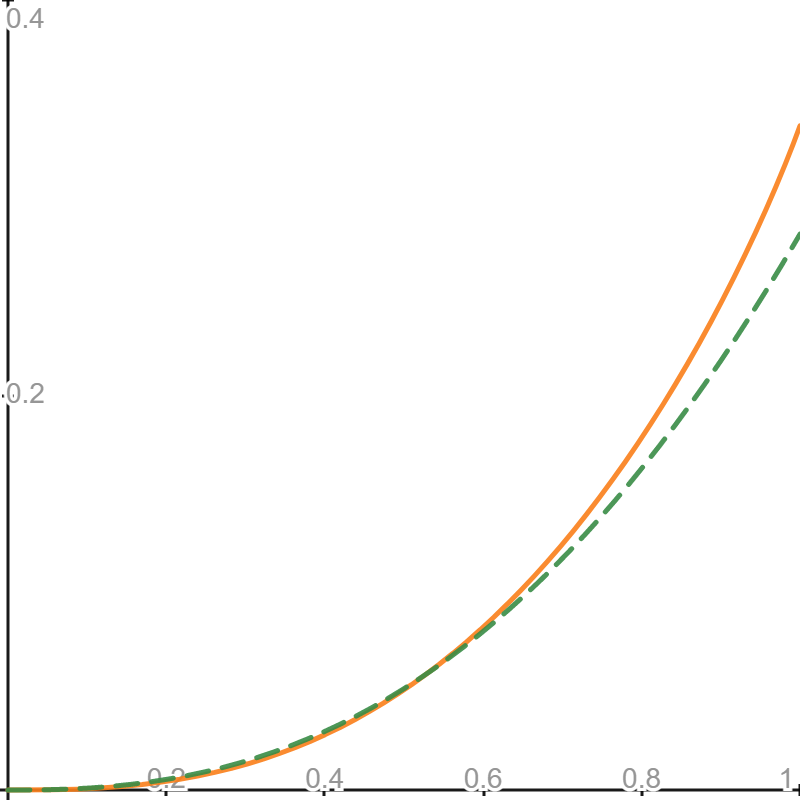
(a) $\Lambda_{1}^{3}$ (solid) and $\Lambda^{3}_{2(2.2)}$ (dashed)

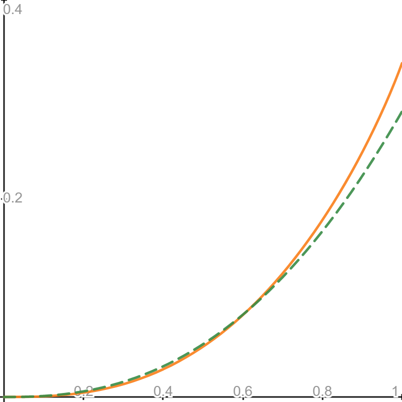
(b) $\Lambda_{1}^{3}$ (solid) and $\Lambda_{2(2.3)}^{3}$ (dashed)

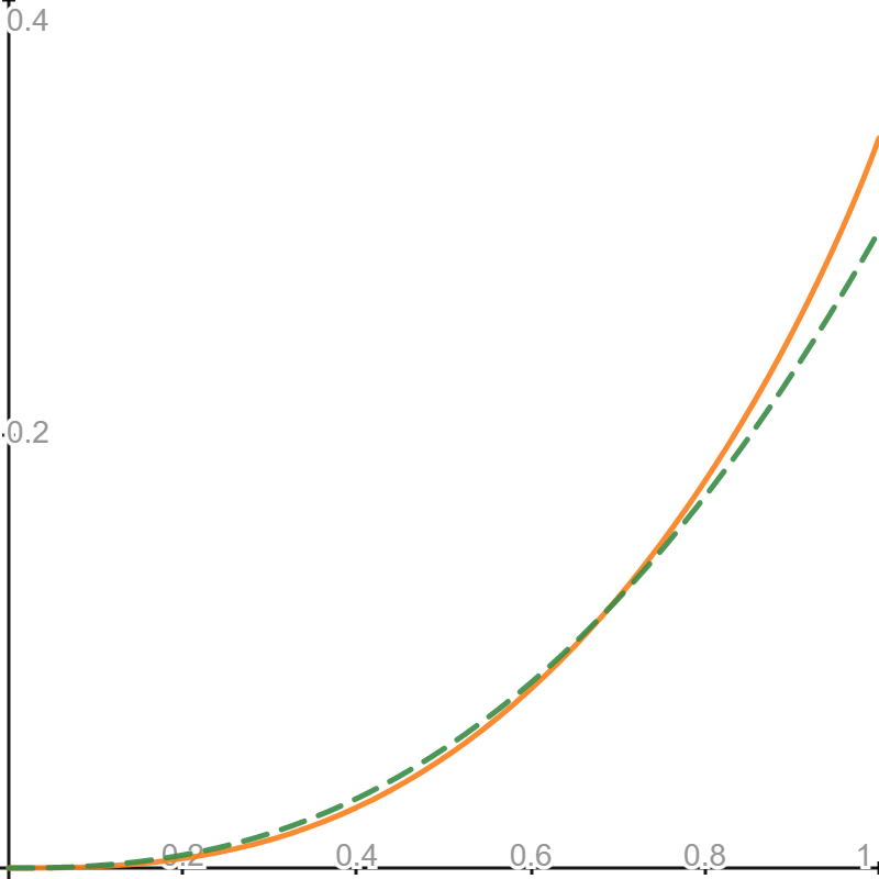
(c) $\Lambda_{1}^{3}$ (solid) and $\Lambda_{2(2.4)}^{3}$ (dashed)

(d) $\Lambda_{1}^{3}$ (solid) and $\Lambda_{2(2.5)}^{3}$ (dashed)

Table C.1: Estimations and Coverage Rates for $3$UISDC (Independent Samples)

DGP	$c_{3}^{u}(F_{1},F_{2})$	$n_{1}$	$n_{2}$	Mean	Bias	SE	RMSE	$t_{n}$	CR
(a)	0.06229	200	200	0.1736	0.1113	0.2474	0.2713	0.001	0.6980
		200	500	0.1339	0.0716	0.2040	0.2162	0.001	0.7190
		200	1000	0.1127	0.0504	0.1797	0.1866	0.001	0.6960
		1000	2000	0.0777	0.0154	0.0762	0.0778	0.001	0.8430
		10000	10000	0.0633	0.0010	0.0219	0.0219	0.001	0.9220
(b)	0.14052	200	200	0.2546	0.1141	0.2916	0.3131	0.001	0.6850
		200	500	0.2130	0.0725	0.2566	0.2666	0.001	0.7210
		200	1000	0.1882	0.0476	0.2351	0.2398	0.001	0.7080
		1000	2000	0.1577	0.0172	0.1206	0.1218	0.001	0.8510
		10000	10000	0.1404	-0.0001	0.0406	0.0406	0.001	0.9190
(c)	0.26581	200	200	0.3461	0.0803	0.3231	0.3329	0.001	0.6680
		200	500	0.3077	0.0419	0.2961	0.2990	0.001	0.7140
		200	1000	0.2819	0.0161	0.2801	0.2806	0.001	0.7030
		1000	2000	0.2735	0.0076	0.1630	0.1631	0.001	0.8620
		10000	10000	0.2617	-0.0041	0.0616	0.0618	0.001	0.9200
(d)	0.42840	200	200	0.4418	0.0134	0.3389	0.3392	0.001	0.6690
		200	500	0.4117	-0.0167	0.3174	0.3178	0.001	0.7010
		200	1000	0.3868	-0.0416	0.3086	0.3114	0.001	0.6970
		1000	2000	0.4139	-0.0145	0.1899	0.1905	0.001	0.8660
		10000	10000	0.4177	-0.0107	0.0761	0.0768	0.001	0.9210

Table C.2: Estimations and Coverage Rates for $3$UISDC (Matched Pairs)

DGP	$c_{3}^{u}(F_{1},F_{2})$	$n_{1}$	$n_{2}$	Mean	Bias	SE	RMSE	$t_{n}$	CR
(a)	0.06229	200	200	0.1212	0.0589	0.1711	0.1809	0.001	0.7690
		500	500	0.1386	0.0764	0.1308	0.1515	0.001	0.9320
		1000	1000	0.0912	0.0289	0.0732	0.0787	0.001	0.9430
		2000	2000	0.0709	0.0086	0.0422	0.0431	0.001	0.9350
		10000	10000	0.0642	0.0019	0.0166	0.0167	2.4	0.9510
(b)	0.14052	200	200	0.1998	0.0593	0.2236	0.2313	0.001	0.7930
		500	500	0.2453	0.1048	0.1785	0.2070	0.001	0.9400
		1000	1000	0.1863	0.0458	0.1180	0.1266	0.001	0.9490
		2000	2000	0.1519	0.0114	0.0729	0.0738	0.001	0.9510
		10000	10000	0.1423	0.0018	0.0305	0.0306	3.7	0.9510
(c)	0.26581	200	200	0.2972	0.0314	0.2656	0.2674	0.001	0.8020
		500	500	0.3783	0.1125	0.2106	0.2388	0.001	0.9180
		1000	1000	0.3221	0.0563	0.1576	0.1674	0.001	0.9480
		2000	2000	0.2756	0.0098	0.1046	0.1050	1	0.9380
		10000	10000	0.2655	-0.0004	0.0462	0.0462	6.7	0.9500
(d)	0.42840	200	200	0.4061	-0.0223	0.2900	0.2909	0.001	0.8030
		500	500	0.5203	0.0919	0.2186	0.2371	0.001	0.8990
		1000	1000	0.4810	0.0526	0.1761	0.1838	0.001	0.9320
		2000	2000	0.4305	0.0021	0.1244	0.1244	1.5	0.9500
		10000	10000	0.4236	-0.0048	0.0567	0.0569	15.6	0.9550

C.2 Stochastic Dominance Coefficient

We let $X^{1}$ and $X^{2}$ be random variables such that

$$X^{1}=\begin{cases}0.25&\text{ with probability }1/\beta,\\ 1&\text{ with probability }1-1/\beta,\end{cases}\text{ and }X^{2}=\begin{cases}0.5&\text{ with probability }2/3,\\ 0.75&\text{ with probability }1/3,\end{cases}$$

with $\beta\in\{2,4,6,8\}$. Figure C.2 displays the CDF curves $F_{1(\beta)}$ and $F_{2}$ corresponding to the above DGPs. The SDC $c_{1}(F_{1},F_{2})=$ $0.081081$, $0.11111$, $0.17647$, and $0.42857$, respectively for $\beta=$ $8$, $6$, $4$, and $2$. We choose the tuning parameter from $t_{n}\in(0,20]$. For independent samples, we let

$$(n_{1},n_{2})\in\{(100,100),(100,200),(100,500),(200,500),(1000,1000)\}.$$

For matched pairs, we let

$$(n_{1},n_{2})\in\{(100,100),(200,200),(300,300),(500,500),(1000,1000)\}.$$

Tables C.3 and C.4 show the simulation results for independent samples and matched pairs which are similar to those in Tables 3.1 and 3.2. For all DGPs, as $n_{1}$ and $n_{2}$ increase, Mean gets close to $c_{1}(F_{1},F_{2})$, Bias decreases to $0$, and both SE and RMSE decrease; under appropriate choices of $t_{n}$, CR approaches to $95\%$.

Figure C.2: Distribution Curves for Four DGPs

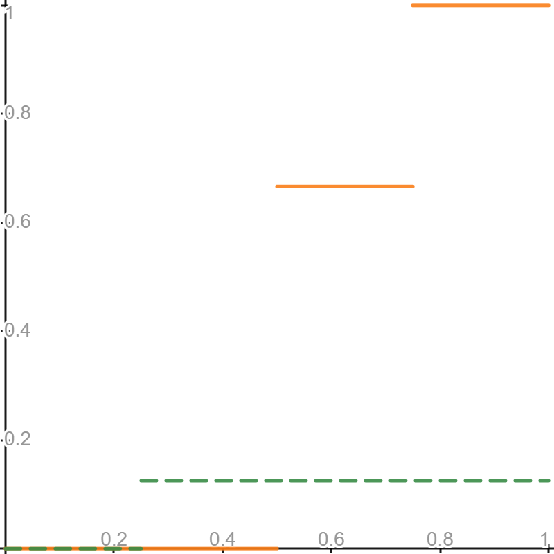
(a) $F_{1(8)}$ (dashed) and $F_{2}$ (solid)

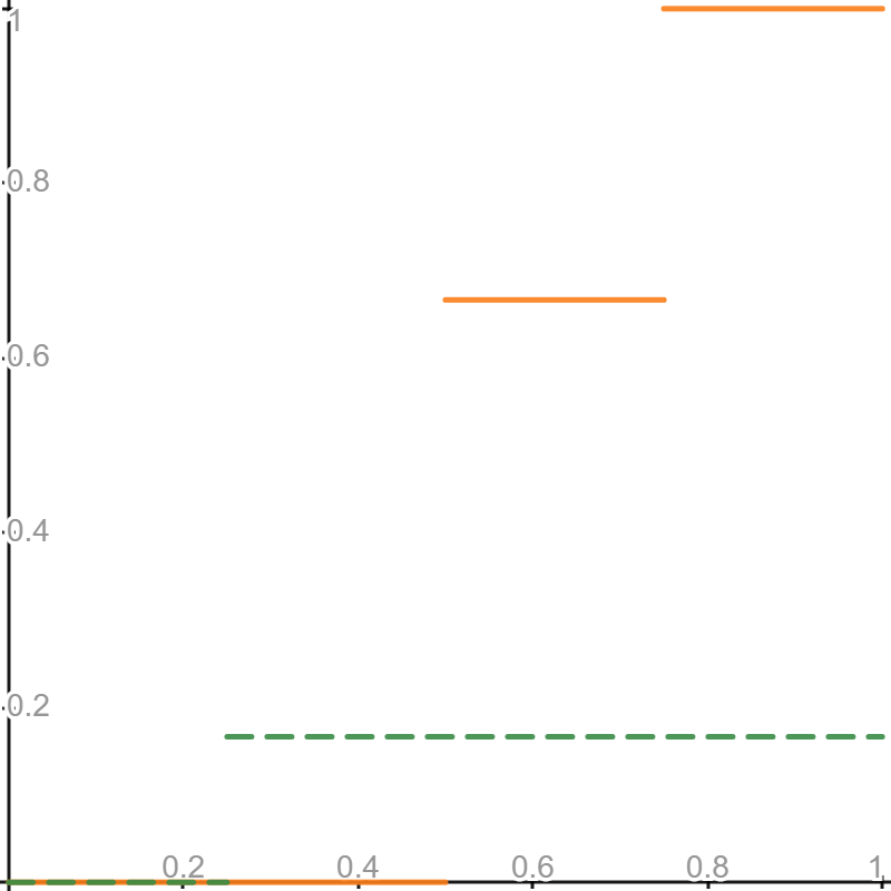
(b) $F_{1(6)}$ (dashed) and $F_{2}$ (solid)

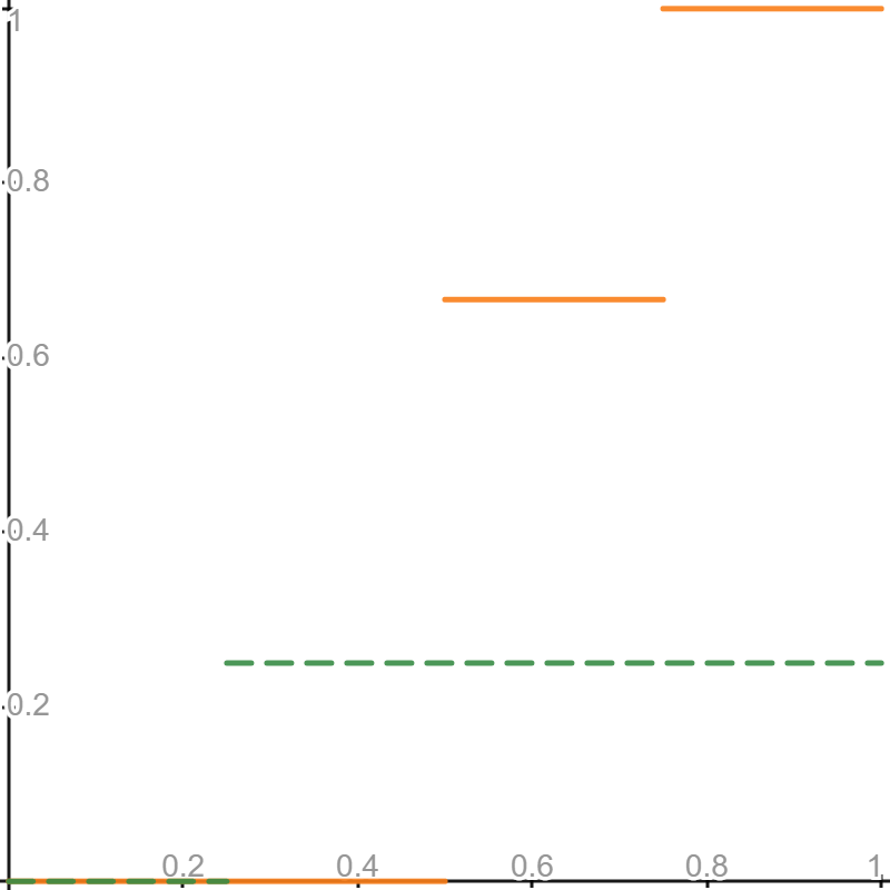
(c) $F_{1(4)}$ (dashed) and $F_{2}$ (solid)

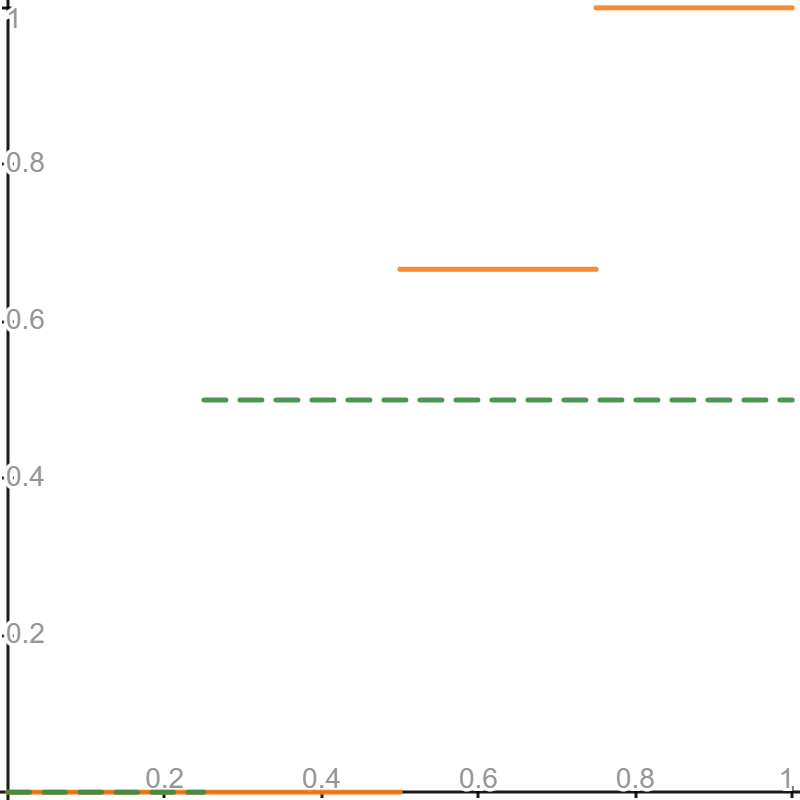
(d) $F_{1(2)}$ (dashed) and $F_{2}$ (solid)

Table C.3: Estimations and Coverage Rates for SDC (Independent Samples)

DGP	$c_{1}(F_{1},F_{2})$	$n_{1}$	$n_{2}$	Mean	Bias	SE	RMSE	$t_{n}$	CR
(a)	0.08108	100	100	0.0826	0.0016	0.0241	0.0241	0.001	0.9380
		100	200	0.0823	0.0012	0.0236	0.0236	0.001	0.9350
		100	500	0.0812	0.0002	0.0229	0.0229	0.001	0.9330
		200	500	0.0819	0.0009	0.0171	0.0171	0.001	0.9270
		1000	1000	0.0812	0.0001	0.0073	0.0073	0.001	0.9490
(b)	0.11111	100	100	0.1130	0.0019	0.0290	0.0290	0.001	0.9410
		100	200	0.1114	0.0003	0.0276	0.0276	0.001	0.9450
		100	500	0.1119	0.0008	0.0269	0.0269	0.001	0.9540
		200	500	0.1115	0.0004	0.0196	0.0196	0.001	0.9440
		1000	1000	0.1111	0.0000	0.0086	0.0086	0.001	0.9500
(c)	0.17647	100	100	0.1804	0.0039	0.0386	0.0388	2.7	0.9470
		100	200	0.1781	0.0016	0.0370	0.0371	3.0	0.9390
		100	500	0.1766	0.0001	0.0361	0.0361	3.9	0.9490
		200	500	0.1774	0.0010	0.0251	0.0251	5.8	0.9510
		1000	1000	0.1767	0.0002	0.0113	0.0113	12.0	0.9510
(d)	0.42857	100	100	0.4326	0.0040	0.0652	0.0653	0.001	0.9470
		100	200	0.4355	0.0069	0.0657	0.0660	0.001	0.9390
		100	500	0.4317	0.0032	0.0634	0.0635	0.001	0.9410
		200	500	0.4302	0.0016	0.0443	0.0443	0.001	0.9450
		1000	1000	0.4284	-0.0002	0.0209	0.0209	5.0	0.9500

Table C.4: Estimations and Coverage Rates for SDC (Matched Pairs)

DGP	$c_{1}(F_{1},F_{2})$	$n_{1}$	$n_{2}$	Mean	Bias	SE	RMSE	$t_{n}$	CR
(a)	0.08108	100	100	0.0824	0.0013	0.0233	0.0234	0.001	0.9450
		200	200	0.0817	0.0006	0.0164	0.0164	0.001	0.9450
		300	300	0.0816	0.0006	0.0138	0.0138	0.001	0.9410
		500	500	0.0815	0.0004	0.0101	0.0101	7.3	0.9520
		1000	1000	0.0815	0.0004	0.0077	0.0077	7.3	0.9390
(b)	0.11111	100	100	0.1126	0.0015	0.0278	0.0278	3.3	0.9530
		200	200	0.1113	0.0002	0.0190	0.0190	3.3	0.9470
		300	300	0.1111	0.0000	0.0158	0.0158	6.4	0.9510
		500	500	0.1116	0.0005	0.0114	0.0115	9.0	0.9510
		1000	1000	0.1117	0.0006	0.0089	0.0089	9.0	0.9490
(c)	0.17647	100	100	0.1796	0.0031	0.0359	0.0361	4.6	0.9480
		200	200	0.1768	0.0003	0.0248	0.0248	6.9	0.9490
		300	300	0.1766	0.0001	0.0203	0.0203	8.7	0.9530
		500	500	0.1768	0.0003	0.0152	0.0152	11.7	0.9510
		1000	1000	0.1769	0.0004	0.0110	0.0110	16.9	0.9500
(d)	0.42857	100	100	0.4298	0.0012	0.0519	0.0519	4.9	0.9490
		200	200	0.4299	0.0013	0.0371	0.0371	6.5	0.9550
		300	300	0.4294	0.0009	0.0292	0.0292	7.9	0.9460
		500	500	0.4289	0.0004	0.0229	0.0229	10.0	0.9480
		1000	1000	0.4299	0.0014	0.0156	0.0157	13.9	0.9510

C.3 Tuning Parameter Selection

In the above simulations, we compute the confidence intervals for all $t_{n}$ from some prespecified set and display the values that yield the best results. We now propose an empirical way of selecting $t_{n}$ in practice. Let $t_{n}$ be selected from a set $S_{t}$ which is sufficiently large. Suppose that we observe the data $\{X_{i}^{1}\}_{i=1}^{n_{1}}$ and $\{X_{i}^{2}\}_{i=1}^{n_{2}}$. We then take the empirical distributions of $\{X_{i}^{1}\}_{i=1}^{n_{1}}$ and $\{X_{i}^{2}\}_{i=1}^{n_{2}}$ as the DGP to generate the data in the simulations and compute the dominance coefficient $c$ based on the empirical distributions of $\{X_{i}^{1}\}_{i=1}^{n_{1}}$ and $\{X_{i}^{2}\}_{i=1}^{n_{2}}$. We take this $c$ as the true value of the coefficient we are interested in. Then we follow the previous simulation procedure to compute the bootstrap confidence intervals for every value of $t_{n}$. Finally, we pick the value $t_{n}$ which yields the coverage rate that is closest to $1-\alpha$, and use this value to construct the bootstrap confidence intervals in the application.

Appendix D Proofs

D.1 Proofs for Section 2

Proof of Lemma 2.1. If (2.4) holds with some $c\in[0,\varepsilon]$ for some $\varepsilon\in[0,1/2)$, then clearly $F_{1}$ $\varepsilon$-ALD $F_{2}$ by definition. If $F_{1}$ $\varepsilon$-ALD $F_{2}$ for some $\varepsilon\in[0,1/2)$, then we can find

$$c=\frac{\int_{S(F_{1},F_{2})}\left(L_{2}\left(p\right)-L_{1}\left(p\right)\right)\mathrm{d}p}{\int_{0}^{1}\left|L_{2}\left(p\right)-L_{1}\left(p\right)\right|\mathrm{d}p}$$

that satisfies (2.4).   

Proof of Lemma 2.2. Suppose that

$$\int_{S(F_{1},F_{2})}\left(L_{2}\left(p\right)-L_{1}\left(p\right)\right)\mathrm{d}p>c\left(L_{1},L_{2}\right)\int_{0}^{1}\left|L_{2}\left(p\right)-L_{1}\left(p\right)\right|\mathrm{d}p,$$

then there is some $\delta>0$ such that

$$\int_{S(F_{1},F_{2})}\left(L_{2}\left(p\right)-L_{1}\left(p\right)\right)\mathrm{d}p=\left\{c\left(L_{1},L_{2}\right)+\delta\right\}\int_{0}^{1}\left|L_{2}\left(p\right)-L_{1}\left(p\right)\right|\mathrm{d}p.$$

For all $\varepsilon\in\left[0,1\right]$ with

$$\int_{S(F_{1},F_{2})}\left(L_{2}\left(p\right)-L_{1}\left(p\right)\right)\mathrm{d}p\leq\int_{0}^{1}\left|L_{2}\left(p\right)-L_{1}\left(p\right)\right|\mathrm{d}p,$$

we have that $\varepsilon\geq c\left(L_{1},L_{2}\right)+\delta$. It then follows that

$$c\left(L_{1},L_{2}\right)<c\left(L_{1},L_{2}\right)+\frac{\delta}{2}<\varepsilon$$

for all $\varepsilon$ such that $\int_{S(F_{1},F_{2})}\left(L_{2}\left(p\right)-L_{1}\left(p\right)\right)\mathrm{d}p\leq\varepsilon\int_{0}^{1}\left|L_{2}\left(p\right)-L_{1}\left(p\right)\right|\mathrm{d}p$, which contradicts the definition of $c\left(L_{1},L_{2}\right)$. Thus, we have

$$\int_{S(F_{1},F_{2})}\left(L_{2}\left(p\right)-L_{1}\left(p\right)\right)\mathrm{d}p\leq c\left(L_{1},L_{2}\right)\int_{0}^{1}\left|L_{2}\left(p\right)-L_{1}\left(p\right)\right|\mathrm{d}p.$$

If there is some other $c$ such that $c<c\left(L_{1},L_{2}\right)$ and

$$\int_{S(F_{1},F_{2})}\left(L_{2}\left(p\right)-L_{1}\left(p\right)\right)\mathrm{d}p\leq c\int_{0}^{1}\left|L_{2}\left(p\right)-L_{1}\left(p\right)\right|\mathrm{d}p,$$

then the definition of $c\left(L_{1},L_{2}\right)$ is contradicted. Thus, $c(L_{1},L_{2})$ is the smallest $\varepsilon$ such that (2.3) holds. If $c\left(L_{1},L_{2}\right)=0$, then $\int_{S(F_{1},F_{2})}\left(L_{2}\left(p\right)-L_{1}\left(p\right)\right)\mathrm{d}p=0$. By (1.1), (2.7) holds. If $c\left(L_{1},L_{2}\right)\neq 0$, then $\int_{S(F_{1},F_{2})}\left(L_{2}\left(p\right)-L_{1}\left(p\right)\right)\mathrm{d}p\neq 0$ and clearly $\int_{0}^{1}|L_{2}(p)-L_{1}(p)|\mathrm{d}p\neq 0$. Then (2.7) holds since $c(L_{1},L_{2})$ is the smallest $\varepsilon$ such that (2.3) holds.

If $c\left(L_{1},L_{2}\right)=0$, then $\int_{S(F_{1},F_{2})}\left(L_{2}\left(p\right)-L_{1}\left(p\right)\right)\mathrm{d}p=0$ which implies that $F_{1}$ Lorenz dominates $F_{2}$. If $F_{1}$ Lorenz dominates $F_{2}$, then $\int_{S(F_{1},F_{2})}\left(L_{2}\left(p\right)-L_{1}\left(p\right)\right)\mathrm{d}p=0$ and thus $c\left(L_{1},L_{2}\right)=0$. If $c\left(L_{1},L_{2}\right)=1$, then $\int_{S(F_{2},F_{1})}\left(L_{1}\left(p\right)-L_{2}\left(p\right)\right)\mathrm{d}p=0$ which implies that $F_{2}$ Lorenz dominates $F_{1}$.

It is clear that

$$\int_{0}^{1}\left|L_{2}\left(p\right)-L_{1}\left(p\right)\right|\mathrm{d}p =\int_{0}^{1}\phi\left(p\right)1\left\{\phi\left(p\right)\geq 0\right\}\mathrm{d}p+\int_{0}^{1}-\phi\left(p\right)1\left\{\phi\left(p\right)<0\right\}\mathrm{d}p$$

$$=\int_{0}^{1}\max\left\{\phi\left(p\right),0\right\}\mathrm{d}p+\int_{0}^{1}\max\left\{-\phi\left(p\right),0\right\}\mathrm{d}p.$$

So by (1.1), (2.7) holds. If $c\left(L_{1},L_{2}\right)\in(0,1]$, then by (2.7),

$$c\left(L_{2},L_{1}\right)=\frac{\int_{0}^{1}\max\left\{-\phi\left(p\right),0\right\}\mathrm{d}p}{\int_{0}^{1}\max\left\{\phi\left(p\right),0\right\}\mathrm{d}p+\int_{0}^{1}\max\left\{-\phi\left(p\right),0\right\}\mathrm{d}p}=1-c\left(L_{1},L_{2}\right).$$

 

Proof of Proposition 2.1. For every $c\left(L_{1},L_{2}\right)\in(0,1/2)$, by Lemma 2.2 and Proposition 1 of zheng2018almost, $F_{1}$ $\varepsilon$-ALD $F_{2}$ for every $\varepsilon\in[c\left(L_{1},L_{2}\right),1/2)$ and $I\left(F_{1},\theta\right)\leq I\left(F_{2},\theta\right)$ for all $I\left(\cdot,\theta\right)\in\mathscr{B}^{\ast}\left(\varepsilon\right)$. If $c\left(L_{1},L_{2}\right)=0$, then by Lemma 2.2, $F_{1}$ Lorenz dominates $F_{2}$ and the claim is clearly true.   

Proof of Proposition 2.2. The proof closely follows the strategies of the proofs of Theorem 1 of leshno2002preferred and Theorem 3.1A of aaberge2009ranking. Using integration by parts, we can show that for every $P\in\mathrm{P}$,

$$J_{P}\left(L_{2}\right)-J_{P}\left(L_{1}\right)=\int_{0}^{1}P^{\prime}\left(t\right)\mathrm{d}L_{1}\left(t\right)-\int_{0}^{1}P^{\prime}\left(t\right)\mathrm{d}L_{2}\left(t\right)$$

$$= \,-\int_{0}^{1}P^{\left(2\right)}\left(t\right)\mathrm{d}L_{1}^{2}\left(t\right)+\int_{0}^{1}P^{\left(2\right)}\left(t\right)\mathrm{d}L_{2}^{2}\left(t\right)$$

$$= \,-P^{\left(2\right)}\left(t\right)L_{1}^{2}\left(t\right)|_{0}^{1}+P^{\left(2\right)}\left(t\right)L_{2}^{2}\left(t\right)|_{0}^{1}+\int_{0}^{1}P^{\left(3\right)}\left(t\right)\mathrm{d}L_{1}^{3}\left(t\right)-\int_{0}^{1}P^{\left(3\right)}\left(t\right)\mathrm{d}L_{2}^{3}\left(t\right)$$

$$= \,\sum_{j=2}^{m}\left(-1\right)^{j-1}P^{\left(j\right)}\left(1\right)\left(L_{1}^{j}\left(1\right)-L_{2}^{j}\left(1\right)\right)+\int_{0}^{1}\left(-1\right)^{m}P^{\left(m+1\right)}\left(t\right)\left(L_{1}^{m}\left(t\right)-L_{2}^{m}\left(t\right)\right)\mathrm{d}t.$$

If $P\in\mathrm{P}_{m}\left(\varepsilon_{m}\right)$, then $\sum_{j=2}^{m}\left(-1\right)^{j-1}P^{\left(j\right)}\left(1\right)(L_{1}^{j}\left(1\right)-L_{2}^{j}\left(1\right))=0$. For every $m\geq 2$, let $r_{U}=\sup_{t}\{\left(-1\right)^{m}P^{\left(m+1\right)}\left(t\right)\}$ and $r_{L}=\inf_{t}\{\left(-1\right)^{m}P^{\left(m+1\right)}\left(t\right)\}$. Also, let $S=\{t\in\left[0,1\right]:L_{1}^{m}\left(t\right)-L_{2}^{m}\left(t\right)<0\}$. It then follows that

$$\int_{0}^{1}\left(-1\right)^{m}P^{\left(m+1\right)}\left(t\right)\left(L_{1}^{m}\left(t\right)-L_{2}^{m}\left(t\right)\right)\mathrm{d}t$$

$$\geq \,r_{U}\int_{S}\left(L_{1}^{m}\left(t\right)-L_{2}^{m}\left(t\right)\right)\mathrm{d}t+r_{L}\int_{S^{c}}\left(L_{1}^{m}\left(t\right)-L_{2}^{m}\left(t\right)\right)\mathrm{d}t$$

$$= \,r_{U}\int_{S}\left(L_{1}^{m}\left(t\right)-L_{2}^{m}\left(t\right)\right)\mathrm{d}t-r_{L}\int_{S}\left(L_{1}^{m}\left(t\right)-L_{2}^{m}\left(t\right)\right)\mathrm{d}t$$

$$+r_{L}\int_{S}\left(L_{1}^{m}\left(t\right)-L_{2}^{m}\left(t\right)\right)\mathrm{d}t+r_{L}\int_{S^{c}}\left(L_{1}^{m}\left(t\right)-L_{2}^{m}\left(t\right)\right)\mathrm{d}t$$

$$= \,\left(r_{U}+r_{L}\right)\int_{S}\left(L_{1}^{m}\left(t\right)-L_{2}^{m}\left(t\right)\right)\mathrm{d}t+r_{L}\int_{0}^{1}\left|L_{1}^{m}\left(t\right)-L_{2}^{m}\left(t\right)\right|\mathrm{d}t$$

$$= \,-\left(r_{U}+r_{L}\right)\int_{0}^{1}\max\left(L_{2}^{m}\left(t\right)-L_{1}^{m}\left(t\right),0\right)\mathrm{d}t+r_{L}\int_{0}^{1}\left|L_{1}^{m}\left(t\right)-L_{2}^{m}\left(t\right)\right|\mathrm{d}t$$

$$\geq \,-\left(r_{U}+r_{L}\right)\varepsilon_{m}\int_{0}^{1}\left|L_{1}^{m}\left(t\right)-L_{2}^{m}\left(t\right)\right|\mathrm{d}t+r_{L}\int_{0}^{1}\left|L_{1}^{m}\left(t\right)-L_{2}^{m}\left(t\right)\right|\mathrm{d}t.$$

With $P\in\mathrm{P}_{m}\left(\varepsilon_{m}\right)$, we have

$$r_{U}\leq r_{L}\left(\frac{1}{\varepsilon_{m}}-1\right)\Leftrightarrow\left(r_{U}+r_{L}\right)\varepsilon_{m}\leq r_{L},$$

which implies $J_{P}\left(L_{2}\right)-J_{P}\left(L_{1}\right)\geq 0$.

If $L_{1}^{j}\left(1\right)-L_{2}^{j}\left(1\right)\geq 0$ for all $j\leq m$, then for every $P\in\mathrm{P}_{m}^{\prime}\left(\varepsilon_{m}\right)$, we have that $\sum_{j=2}^{m}\left(-1\right)^{j-1}P^{\left(j\right)}\left(1\right)(L_{1}^{j}\left(1\right)-L_{2}^{j}\left(1\right))\geq 0$ and the result follows.   

Proof of Lemma 2.3. The proof is similar to that of Lemma 2.2.   

Proof of Proposition 2.3. The results directly follow from Lemma 2.3 and Proposition 2.2.   

Proof of Proposition 2.4. The proof closely follows the strategies of the proofs of Theorem 1 of leshno2002preferred and Theorem 3.1B of aaberge2009ranking. Clearly, for $m\geq 3$, we have that ${\mathrm{d}\tilde{L}_{j}^{m}\left(p\right)}/{\mathrm{d}p}=-\tilde{L}_{j}^{m-1}\left(p\right)$. Also,

$$\tilde{L}_{j}^{2}\left(p\right)=\int_{p}^{1}\left(1-L_{j}\left(t\right)\right)\mathrm{d}t=\left(1-p\right)-\int_{0}^{1}L_{j}\left(t\right)\mathrm{d}t+L_{j}^{2}\left(p\right),$$

and it follows that ${\mathrm{d}\tilde{L}_{j}^{2}\left(p\right)}/{\mathrm{d}p}=-1+{\mathrm{d}L_{j}^{2}\left(p\right)}/{\mathrm{d}p}$. Then we have that for every $P\in\mathrm{P}$,

$$J_{P}\left(L_{2}\right)-J_{P}\left(L_{1}\right)=\int_{0}^{1}P^{\prime}\left(t\right)\mathrm{d}L_{1}\left(t\right)-\int_{0}^{1}P^{\prime}\left(t\right)\mathrm{d}L_{2}\left(t\right)$$

$$= \,-\int_{0}^{1}P^{\left(2\right)}\left(t\right)\mathrm{d}L_{1}^{2}\left(t\right)+\int_{0}^{1}P^{\left(2\right)}\left(t\right)\mathrm{d}L_{2}^{2}\left(t\right)=-\int_{0}^{1}P^{\left(2\right)}\left(t\right)\mathrm{d}\tilde{L}_{1}^{2}\left(t\right)+\int_{0}^{1}P^{\left(2\right)}\left(t\right)\mathrm{d}\tilde{L}_{2}^{2}\left(t\right)$$

$$= \,-P^{\left(2\right)}\left(t\right)\tilde{L}_{1}^{2}\left(t\right)|_{0}^{1}+P^{\left(2\right)}\left(t\right)\tilde{L}_{2}^{2}\left(t\right)|_{0}^{1}-\int_{0}^{1}P^{\left(3\right)}\left(t\right)\mathrm{d}\tilde{L}_{1}^{3}\left(t\right)+\int_{0}^{1}P^{\left(3\right)}\left(t\right)\mathrm{d}\tilde{L}_{2}^{3}\left(t\right)$$

$$= \,\sum_{j=2}^{m}P^{\left(j\right)}\left(0\right)\left(\tilde{L}_{1}^{j}\left(0\right)-\tilde{L}_{2}^{j}\left(0\right)\right)+\int_{0}^{1}-P^{\left(m+1\right)}\left(t\right)\left(\tilde{L}_{2}^{m}\left(t\right)-\tilde{L}_{1}^{m}\left(t\right)\right)\mathrm{d}t.$$

If $P\in\tilde{\mathrm{P}}_{m}\left(\varepsilon_{m}\right)$, then $\sum_{j=2}^{m}P^{\left(j\right)}\left(0\right)(\tilde{L}_{1}^{j}\left(0\right)-L_{2}^{j}\left(0\right))=0$. Let $r_{U}=\sup_{t}\{-P^{\left(m+1\right)}\left(t\right)\}$ and $r_{L}=\inf_{t}\{-P^{\left(m+1\right)}\left(t\right)\}$. Also, let $S=\{t\in\left[0,1\right]:\tilde{L}_{1}^{m}\left(t\right)-\tilde{L}_{2}^{m}\left(t\right)>0\}$. It then follows that

$$\int_{0}^{1}-P^{\left(m+1\right)}\left(t\right)\left(\tilde{L}_{2}^{m}\left(t\right)-\tilde{L}_{1}^{m}\left(t\right)\right)\mathrm{d}t$$

$$\geq \,r_{U}\int_{S}\left(\tilde{L}_{2}^{m}\left(t\right)-\tilde{L}_{1}^{m}\left(t\right)\right)\mathrm{d}t+r_{L}\int_{S^{c}}\left(\tilde{L}_{2}^{m}\left(t\right)-\tilde{L}_{1}^{m}\left(t\right)\right)\mathrm{d}t$$

$$= \,r_{U}\int_{S}\left(\tilde{L}_{2}^{m}\left(t\right)-\tilde{L}_{1}^{m}\left(t\right)\right)\mathrm{d}t-r_{L}\int_{S}\left(\tilde{L}_{2}^{m}\left(t\right)-\tilde{L}_{1}^{m}\left(t\right)\right)\mathrm{d}t$$

$$+r_{L}\int_{S}\left(\tilde{L}_{2}^{m}\left(t\right)-\tilde{L}_{1}^{m}\left(t\right)\right)\mathrm{d}t+r_{L}\int_{S^{c}}\left(\tilde{L}_{2}^{m}\left(t\right)-\tilde{L}_{1}^{m}\left(t\right)\right)\mathrm{d}t$$

$$= \,\left(r_{U}+r_{L}\right)\int_{S}\left(\tilde{L}_{2}^{m}\left(t\right)-\tilde{L}_{1}^{m}\left(t\right)\right)\mathrm{d}t+r_{L}\int_{0}^{1}\left|\tilde{L}_{1}^{m}\left(t\right)-\tilde{L}_{2}^{m}\left(t\right)\right|\mathrm{d}t$$

$$= \,-\left(r_{U}+r_{L}\right)\int_{0}^{1}\max\left(\tilde{L}_{1}^{m}\left(t\right)-\tilde{L}_{2}^{m}\left(t\right),0\right)\mathrm{d}t+r_{L}\int_{0}^{1}\left|\tilde{L}_{1}^{m}\left(t\right)-\tilde{L}_{2}^{m}\left(t\right)\right|\mathrm{d}t$$

$$\geq \,-\left(r_{U}+r_{L}\right)\varepsilon_{m}\int_{0}^{1}\left|\tilde{L}_{1}^{m}\left(t\right)-\tilde{L}_{2}^{m}\left(t\right)\right|\mathrm{d}t+r_{L}\int_{0}^{1}\left|\tilde{L}_{1}^{m}\left(t\right)-\tilde{L}_{2}^{m}\left(t\right)\right|\mathrm{d}t.$$

With $P\in\tilde{\mathrm{P}}_{m}\left(\varepsilon_{m}\right)$, we have

$$r_{U}\leq r_{L}\left(\frac{1}{\varepsilon_{m}}-1\right)\Leftrightarrow\left(r_{U}+r_{L}\right)\varepsilon_{m}\leq r_{L},$$

which implies $J_{P}\left(L_{2}\right)-J_{P}\left(L_{1}\right)\geq 0$.

If $\tilde{L}_{1}^{j}\left(0\right)-\tilde{L}_{2}^{j}\left(0\right)\leq 0$ for all $j\leq m$, then for every $P\in\tilde{\mathrm{P}}_{m}^{\prime}\left(\varepsilon_{m}\right)$, $\sum_{j=2}^{m}P^{\left(j\right)}\left(0\right)(\tilde{L}_{1}^{j}\left(0\right)-\tilde{L}_{2}^{j}\left(0\right))\geq 0$ and the result follows.   

Proof of Lemma 2.4. The proof is similar to that of Lemma 2.2.   

Proof of Proposition 2.5. The results directly follow from Proposition 2.4.   

Lemma D.1

Let $\mathbb{D}$ be a normed space. Suppose that $\mathcal{F}_{1}:\mathbb{D}\rightarrow\mathbb{R}$ and $\mathcal{F}_{2}:\mathbb{D}\rightarrow\mathbb{R}$ such that $\mathcal{F}_{1}$ and $\mathcal{F}_{2}$ are both Hadamard directionally differentiable at $\phi$ tangentially to some $\mathbb{D}_{0}\subset\mathbb{D}$ with the derivatives $\mathcal{F}_{1\phi}^{\prime}$ and $\mathcal{F}_{2\phi}^{\prime}$. Then we have the following results:

1. The summation $\mathcal{F}_{1}+\mathcal{F}_{2}$ is Hadamard directionally differentiable at $\phi$ such that

   $$\left(\mathcal{F}_{1}+\mathcal{F}_{2}\right)_{\phi}^{\prime}\left(h\right)=\mathcal{F}_{1\phi}^{\prime}\left(h\right)+\mathcal{F}_{2\phi}^{\prime}\left(h\right),\quad h\in\mathbb{D}_{0}.$$

2. The multiplication $\mathcal{F}_{1}\mathcal{F}_{2}$ is Hadamard directionally differentiable at $\phi$ such that

   $$\left(\mathcal{F}_{1}\mathcal{F}_{2}\right)_{\phi}^{\prime}\left(h\right)=\mathcal{F}_{1\phi}^{\prime}\left(h\right)\mathcal{F}_{2}\left(\phi\right)+\mathcal{F}_{1}\left(\phi\right)\mathcal{F}_{2\phi}^{\prime}\left(h\right),\quad h\in\mathbb{D}_{0}.$$

3. If $\mathcal{F}_{1}\left(\phi\right)\neq 0$, then the inverse $1/\mathcal{F}_{1}$ is Hadamard directionally differentiable at $\phi$ such that

   $$\left(\frac{1}{\mathcal{F}_{1}}\right)_{\phi}^{\prime}\left(h\right)=-\frac{\mathcal{F}_{1\phi}^{\prime}\left(h\right)}{\mathcal{F}_{1}\left(\phi\right)^{2}},\quad h\in\mathbb{D}_{0}.$$

Proof of Lemma D.1. Let $t_{n}\downarrow 0$ and $h_{n}\to h\in\mathbb{D}_{0}$ such that $\phi+t_{n}h_{n}\in\mathbb{D}$.

(i). By definition, it is easy to show that

$$\frac{\mathcal{F}_{1}\left(\phi+t_{n}h_{n}\right)+\mathcal{F}_{2}\left(\phi+t_{n}h_{n}\right)-\mathcal{F}_{1}\left(\phi\right)-\mathcal{F}_{2}\left(\phi\right)}{t_{n}}-\mathcal{F}_{1\phi}^{\prime}\left(h\right)-\mathcal{F}_{2\phi}^{\prime}\left(h\right)\rightarrow 0.$$

(ii). First, we have that

$$\frac{\mathcal{F}_{1}\left(\phi+t_{n}h_{n}\right)\mathcal{F}_{2}\left(\phi+t_{n}h_{n}\right)-\mathcal{F}_{1}\left(\phi\right)\mathcal{F}_{2}\left(\phi\right)}{t_{n}}$$

$$= \,\frac{\mathcal{F}_{1}\left(\phi+t_{n}h_{n}\right)\mathcal{F}_{2}\left(\phi+t_{n}h_{n}\right)-\mathcal{F}_{1}\left(\phi\right)\mathcal{F}_{2}\left(\phi+t_{n}h_{n}\right)}{t_{n}}$$

$$+\frac{\mathcal{F}_{1}\left(\phi\right)\mathcal{F}_{2}\left(\phi+t_{n}h_{n}\right)-\mathcal{F}_{1}\left(\phi\right)\mathcal{F}_{2}\left(\phi\right)}{t_{n}}.$$

Then, by the continuity of $\mathcal{F}_{2}$ ($\mathcal{F}_{2}$ is directionally differentiable), we can show that

$$\frac{\mathcal{F}_{1}\left(\phi+t_{n}h_{n}\right)\mathcal{F}_{2}\left(\phi+t_{n}h_{n}\right)-\mathcal{F}_{1}\left(\phi\right)\mathcal{F}_{2}\left(\phi+t_{n}h_{n}\right)}{t_{n}}-\mathcal{F}_{1\phi}^{\prime}\left(h\right)\mathcal{F}_{2}\left(\phi+t_{n}h_{n}\right)$$

$$+\mathcal{F}_{1\phi}^{\prime}\left(h\right)\mathcal{F}_{2}\left(\phi+t_{n}h_{n}\right)-\mathcal{F}_{1\phi}^{\prime}\left(h\right)\mathcal{F}_{2}\left(\phi\right)\rightarrow 0$$

and

$$\frac{\mathcal{F}_{1}\left(\phi\right)\mathcal{F}_{2}\left(\phi+t_{n}h_{n}\right)-\mathcal{F}_{1}\left(\phi\right)\mathcal{F}_{2}\left(\phi\right)}{t_{n}}-\mathcal{F}_{1}\left(\phi\right)\mathcal{F}_{2\phi}^{\prime}\left(h\right)\rightarrow 0.$$

(iii). We first write

$$\frac{1/\mathcal{F}_{1}\left(\phi+t_{n}h_{n}\right)-1/\mathcal{F}_{1}\left(\phi\right)}{t_{n}}=\frac{1}{t_{n}}\frac{\mathcal{F}_{1}\left(\phi\right)-\mathcal{F}_{1}\left(\phi+t_{n}h_{n}\right)}{\mathcal{F}_{1}\left(\phi+t_{n}h_{n}\right)\mathcal{F}_{1}\left(\phi\right)}.$$

Then, by the continuity of $\mathcal{F}_{1}$ ($\mathcal{F}_{1}$ is directionally differentiable), we can show that

$$\frac{1}{t_{n}}\frac{\mathcal{F}_{1}\left(\phi\right)-\mathcal{F}_{1}\left(\phi+t_{n}h_{n}\right)}{\mathcal{F}_{1}\left(\phi+t_{n}h_{n}\right)\mathcal{F}_{1}\left(\phi\right)} -\left(-\frac{\mathcal{F}_{1\phi}^{\prime}\left(h\right)}{\mathcal{F}_{1}\left(\phi+t_{n}h_{n}\right)\mathcal{F}_{1}\left(\phi\right)}\right)$$

$$-\frac{\mathcal{F}_{1\phi}^{\prime}\left(h\right)}{\mathcal{F}_{1}\left(\phi+t_{n}h_{n}\right)\mathcal{F}_{1}\left(\phi\right)}-\left(-\frac{\mathcal{F}_{1\phi}^{\prime}\left(h\right)}{\mathcal{F}_{1}\left(\phi\right)^{2}}\right)\rightarrow 0.$$

 

Proof of Lemma 2.5. We closely follow the proofs of Lemma A.1 of Beare2017improved and Lemma 3.1 of jiang2023nonparametric. First, we have that

$$E\left[\mathbb{G}\left(p\right)\mathbb{G}\left(p^{\prime}\right)\right]=E\left[\left(\mathbb{\lambda}^{1/2}\mathcal{L}_{2}\left(p\right)-\left(1-\lambda\right)^{1/2}\mathcal{L}_{1}\left(p\right)\right)\left(\mathbb{\lambda}^{1/2}\mathcal{L}_{2}\left(p^{\prime}\right)-\left(1-\lambda\right)^{1/2}\mathcal{L}_{1}\left(p^{\prime}\right)\right)\right]$$

$$= \,\lambda E\left[\mathcal{L}_{2}\left(p\right)\mathcal{L}_{2}\left(p^{\prime}\right)\right]-\mathbb{\lambda}^{1/2}\left(1-\lambda\right)^{1/2}E\left[\mathcal{L}_{2}\left(p\right)\mathcal{L}_{1}\left(p^{\prime}\right)\right]-\mathbb{\lambda}^{1/2}\left(1-\lambda\right)^{1/2}E\left[\mathcal{L}_{1}\left(p\right)\mathcal{L}_{2}\left(p^{\prime}\right)\right]$$

$$+\left(1-\lambda\right)E\left[\mathcal{L}_{1}\left(p\right)\mathcal{L}_{1}\left(p^{\prime}\right)\right].$$

For $j=1,2$, $p\in\left[0,1\right]$, and $t\in\left[0,1\right]$, define

$$h_{j,p}\left(t\right)=\frac{1}{\mu_{j}}\left\{L_{j}\left(p\right)-1\left(t\leq p\right)\right\}Q_{j}^{\prime}\left(t\right).$$

Note that the almost sure integrability of $h_{j,p}\mathcal{B}_{j}$ follows from the weak convergence of $n_{j}^{1/2}(\hat{Q}_{j}-Q_{j})\leadsto-Q_{j}^{\prime}\mathcal{B}_{j}$ in $L^{1}\left(\left[0,1\right]\right)$ established by K17. Then we can show that $\mathcal{L}_{j}$ defined in (2.25) satisfies that

$$\mathcal{L}_{j}\left(p\right)=\int_{0}^{1}h_{j,p}\left(t\right)\mathcal{B}_{j}\left(t\right)\mathrm{d}t,\quad p\in\left[0,1\right].$$

Define

$$H_{j,p}\left(u\right)=\int_{0}^{u}h_{j,p}\left(t\right)\mathrm{d}t,\quad p\in\left[0,1\right].$$

For $j,j^{\prime}\in\left\{1,2\right\}$ and $p,p^{\prime}\in\left[0,1\right]$, by Fubini’s theorem,

$$Cov\left(\mathcal{L}_{j}\left(p\right),\mathcal{L}_{j^{\prime}}\left(p^{\prime}\right)\right)=\int_{0}^{1}\int_{0}^{1}h_{j,p}\left(t_{1}\right)h_{j^{\prime},p^{\prime}}\left(t_{2}\right)E\left[\mathcal{B}_{j}\left(t_{1}\right)\mathcal{B}_{j^{\prime}}\left(t_{2}\right)\right]\mathrm{d}t_{1}\mathrm{d}t_{2}.$$

Let $\left(U,V\right)$ be a pair of random variables with joint CDF given by the copula $\mathbf{C}$ in Assumption 2.2(ii). For $j=1$ and $j^{\prime}=2$, $E\left[\mathcal{B}_{1}\left(t_{1}\right)\mathcal{B}_{2}\left(t_{2}\right)\right]=\mathbf{C}\left(t_{1},t_{2}\right)-t_{1}t_{2}$. By Theorem 3.1 of lo2017functional (see also cuadras2002covariance and beare2009generalization),

$$Cov\left(H_{j,p}\left(U\right),H_{j^{\prime},p^{\prime}}\left(V\right)\right)=\int_{0}^{1}\int_{0}^{1}h_{j,p}\left(t_{1}\right)h_{j^{\prime},p^{\prime}}\left(t_{2}\right)\left(\mathbf{C}\left(t_{1},t_{2}\right)-t_{1}t_{2}\right)\mathrm{d}t_{1}\mathrm{d}t_{2}.$$

Then it follows that

$$E\left[\mathcal{L}_{1}\left(p\right)\mathcal{L}_{2}\left(p^{\prime}\right)\right]=Cov\left(\mathcal{L}_{1}\left(p\right),\mathcal{L}_{2}\left(p^{\prime}\right)\right)=Cov\left(H_{1,p}\left(F_{1}\left(X_{i}^{1}\right)\right),H_{2,p^{\prime}}\left(F_{2}\left(X_{i}^{2}\right)\right)\right)$$

$$=Cov\left(\frac{1}{\mu_{1}}\left\{L_{1}\left(p\right)X_{i}^{1}-Q_{1}\left(p\right)\wedge X_{i}^{1}\right\},\frac{1}{\mu_{2}}\left\{L_{2}\left(p^{\prime}\right)X_{i}^{2}-Q_{2}\left(p^{\prime}\right)\wedge X_{i}^{2}\right\}\right).$$

For $j=j^{\prime}$, $E\left[\mathcal{B}_{j}\left(t_{1}\right)\mathcal{B}_{j}\left(t_{2}\right)\right]=t_{1}\wedge t_{2}-t_{1}t_{2}$. By Theorem 3.1 of lo2017functional again,

$$Cov\left(H_{j,p}\left(U\right),H_{j,p^{\prime}}\left(U\right)\right)=\int_{0}^{1}\int_{0}^{1}h_{j,p}\left(t_{1}\right)h_{j,p^{\prime}}\left(t_{2}\right)\left(t_{1}\wedge t_{2}-t_{1}t_{2}\right)\mathrm{d}t_{1}\mathrm{d}t_{2}.$$

Then it follows that

$$E\left[\mathcal{L}_{j}\left(p\right)\mathcal{L}_{j}\left(p^{\prime}\right)\right]=Cov\left(\mathcal{L}_{j}\left(p\right),\mathcal{L}_{j}\left(p^{\prime}\right)\right)=Cov\left(H_{j,p}\left(F_{j}\left(X_{i}^{j}\right)\right),H_{j,p^{\prime}}\left(F_{j}\left(X_{i}^{j}\right)\right)\right)$$

$$=Cov\left(\frac{1}{\mu_{j}}\left\{L_{j}\left(p\right)X_{i}^{j}-Q_{j}\left(p\right)\wedge X_{i}^{j}\right\},\frac{1}{\mu_{j}}\left\{L_{j}\left(p^{\prime}\right)X_{i}^{j}-Q_{j}\left(p^{\prime}\right)\wedge X_{i}^{j}\right\}\right).$$

 

Proof of Lemma 2.6. The results follow from the continuous mapping theorem and Fubini’s theorem (see, for example, Theorem 2.37 of folland2013real).   

Proof of Proposition 2.6. For simplicity of notation, we focus on the case where $m=1$. The proof of general results for $m\geq 2$ and $w\in\{u,d\}$ is similar. We first show the Hadamard differentiability of $\mathcal{F}$. Because $L_{1}$ and $L_{2}$ are continuous in $p$, if $L_{1}(p)\neq L_{2}(p)$ for some $p\in[0,1]$, then $\mathcal{F}_{1}(\phi)+\mathcal{F}_{2}(\phi)>0$. By Lemma D.1, we have that

$$\mathcal{F}_{\phi}^{\prime}\left(h\right)=\left(\frac{\mathcal{F}_{1}}{\mathcal{F}_{1}+\mathcal{F}_{2}}\right)_{\phi}^{\prime}\left(h\right)=\frac{\mathcal{F}_{1\phi}^{\prime}\left(h\right)}{\mathcal{F}_{1}\left(\phi\right)+\mathcal{F}_{2}\left(\phi\right)}-\mathcal{F}_{1}\left(\phi\right)\frac{\mathcal{F}_{1\phi}^{\prime}\left(h\right)+\mathcal{F}_{2\phi}^{\prime}\left(h\right)}{\left(\mathcal{F}_{1}\left(\phi\right)+\mathcal{F}_{2}\left(\phi\right)\right)^{2}}$$

$$= \,\frac{\mathcal{F}_{1\phi}^{\prime}\left(h\right)\left[\mathcal{F}_{1}\left(\phi\right)+\mathcal{F}_{2}\left(\phi\right)\right]-\mathcal{F}_{1}\left(\phi\right)\left[\mathcal{F}_{1\phi}^{\prime}\left(h\right)+\mathcal{F}_{2\phi}^{\prime}\left(h\right)\right]}{\left(\mathcal{F}_{1}\left(\phi\right)+\mathcal{F}_{2}\left(\phi\right)\right)^{2}}=\frac{\mathcal{F}_{1\phi}^{\prime}\left(h\right)\mathcal{F}_{2}\left(\phi\right)-\mathcal{F}_{1}\left(\phi\right)\mathcal{F}_{2\phi}^{\prime}\left(h\right)}{\left(\mathcal{F}_{1}\left(\phi\right)+\mathcal{F}_{2}\left(\phi\right)\right)^{2}}.$$ (D.1)

This implies the continuity of $\mathcal{F}$. By Lemma 3 of BDB14, we have $\hat{c}(L_{1},L_{2})\to c(L_{1},L_{2})$ a.s. With (2.24) and (D.1), by Theorem 2.1 of fang2014inference, (2.30) holds.   

Proof of Proposition 2.7. For simplicity of notation, we focus on the case where $m=1$. The proof of general results for $m\geq 2$ and $w\in\{u,d\}$ is similar. Since $c(L_{1},L_{2})\neq 0$, $L_{1}\neq L_{2}$ and $\mathcal{F}_{1}(\phi)+\mathcal{F}_{2}(\phi)>0$. Let $\varepsilon>0$ and $\mu$ denote the Lebesgue measure in the following. First, we have that

$$\mathbb{P}\left(\mu\left(\widehat{B_{+}\left(\phi\right)}\setminus B_{+}\left(\phi\right)\right)>\varepsilon\right)\leq\mathbb{P}\left(\widehat{B_{+}\left(\phi\right)}\setminus B_{+}\left(\phi\right)\neq\varnothing\right)$$

$$\leq \,\mathbb{P}\left(\sup_{p\in\widehat{B_{+}\left(\phi\right)}\setminus B_{+}\left(\phi\right)}\frac{\sqrt{T_{n}}(\hat{\phi}\left(p\right)-\phi\left(p\right))}{\xi_{0}\vee\hat{\sigma}\left(p\right)}>t_{n}\right)\leq\mathbb{P}\left(\sup_{p\in\left[0,1\right]}\frac{\sqrt{T_{n}}(\hat{\phi}\left(p\right)-\phi\left(p\right))}{\xi_{0}\vee\hat{\sigma}\left(p\right)}>t_{n}\right).$$

Since $\sqrt{T_{n}}(\hat{\phi}-\phi)\leadsto\mathbb{G}$, then by Example 1.4.7 (Slutsky’s lemma) and Theorem 1.3.6 (continuous mapping) of van1996weak,

$$\frac{1}{t_{n}}\sup_{p\in\left[0,1\right]}\frac{\sqrt{T_{n}}(\hat{\phi}\left(p\right)-\phi\left(p\right))}{\xi_{0}\vee\hat{\sigma}\left(p\right)}\leq\frac{1}{t_{n}}\sup_{p\in\left[0,1\right]}\left|\frac{\sqrt{T_{n}}(\hat{\phi}\left(p\right)-\phi\left(p\right))}{\xi_{0}}\right|\leadsto 0.$$

Then by Theorem 1.3.4(iii) of van1996weak, $\mathbb{P}(\mu(\widehat{B_{+}\left(\phi\right)}\setminus B_{+}\left(\phi\right))>\varepsilon)\rightarrow 0$.

By Lemma 3 of BDB14, $\sup_{p\in\left[0,1\right]}|\hat{\phi}\left(p\right)-\phi\left(p\right)|\rightarrow 0$ a.s. For simplicity of notation, let $\hat{\sigma}$ denote $\hat{\sigma}_{1}^{w}$ in the following. In the proof of Lemma A.2 of Beare2017improved, it is shown that $\sup_{p\in[0,1]}\hat{\sigma}(p)$ is bounded by some $C_{\sigma}>0$ a.s. Define

$$A_{\phi}=\left\{\omega\in\Omega:\sup_{p\in\left[0,1\right]}\left|\hat{\phi}_{\omega}\left(p\right)-\phi\left(p\right)\right|\rightarrow 0\right\}\cap\left\{\omega\in\Omega:\sup_{p\in[0,1]}\hat{\sigma}_{\omega}(p)\leq C_{\sigma}\right\},$$

where the subscript ${\omega}$ denotes that the random elements are fixed at $\omega$. Then $\mathbb{P}\left(A_{\phi}\right)=1$. Consider

$$\mathbb{P}\left(\mu\left(B_{+}\left(\phi\right)\setminus\widehat{B_{+}\left(\phi\right)}\right)>\varepsilon\right)=\int 1\left\{\mu\left(B_{+}\left(\phi\right)\setminus\widehat{B_{+}\left(\phi\right)}\right)>\varepsilon\right\}\mathrm{d}\mathbb{P}.$$

For every fixed $\omega\in A_{\phi}$, we have that

$$\mu\left(B_{+}\left(\phi\right)\setminus\widehat{B_{+}\left(\phi\right)}\right)=\int_{\left[0,1\right]}1\left\{p\in B_{+}\left(\phi\right)\setminus\widehat{B_{+}\left(\phi\right)}\right\}\mathrm{d}\mu\left(p\right),$$

where

$$B_{+}\left(\phi\right)\setminus\widehat{B_{+}\left(\phi\right)}=\left\{p\in\left[0,1\right]:\frac{\sqrt{T_{n}}\hat{\phi}_{\omega}\left(p\right)}{\xi_{0}\vee\hat{\sigma}_{\omega}\left(p\right)}\leq t_{n},\phi\left(p\right)>0\right\}.$$

For every $p\in\left[0,1\right]$ such that $\phi\left(p\right)>0$, since $\sup_{p\in\left[0,1\right]}|\hat{\phi}_{\omega}\left(p\right)-\phi\left(p\right)|\rightarrow 0$, then when $n$ is large enough, $\hat{\phi}_{\omega}\left(p\right)>1/2\cdot\phi\left(p\right)$. Since $\hat{\sigma}_{\omega}$ is uniformly bounded and $t_{n}/\sqrt{T_{n}}\rightarrow 0$, we have that ($\omega$ is fixed) for every fixed $p\in[0,1]$,

$$1\left\{p\in B_{+}\left(\phi\right)\setminus\widehat{B_{+}\left(\phi\right)}\right\}\rightarrow 0.$$

Thus, by the dominated convergence theorem ($\omega$ is fixed),

$$\mu\left(B_{+}\left(\phi\right)\setminus\widehat{B_{+}\left(\phi\right)}\right)=\int_{\left[0,1\right]}1\left\{p\in B_{+}\left(\phi\right)\setminus\widehat{B_{+}\left(\phi\right)}\right\}\mathrm{d}\mu\left(p\right)\rightarrow 0.$$

This implies that for every $\omega\in A_{\phi}$,

$$1\left\{\mu\left(B_{+}\left(\phi\right)\setminus\widehat{B_{+}\left(\phi\right)}\right)>\varepsilon\right\}\rightarrow 0.$$

Then by the dominated convergence theorem again,

$$\mathbb{P}\left(\mu\left(B_{+}\left(\phi\right)\setminus\widehat{B_{+}\left(\phi\right)}\right)>\varepsilon\right)=\int 1\left\{\mu\left(B_{+}\left(\phi\right)\setminus\widehat{B_{+}\left(\phi\right)}\right)>\varepsilon\right\}\mathrm{d}\mathbb{P}\rightarrow 0.$$

Similarly, we can show that

$$\mathbb{P}\left(\mu\left(\widehat{B_{+}\left(-\phi\right)}\setminus B_{+}\left(-\phi\right)\right)>\varepsilon\right)\rightarrow 0\text{ and }\mathbb{P}\left(\mu\left(B_{+}\left(-\phi\right)\setminus\widehat{B_{+}\left(-\phi\right)}\right)>\varepsilon\right)\rightarrow 0.$$

In addition,

$$\mathbb{P}\left(\mu\left(B_{0}\left(\phi\right)\setminus\widehat{B_{0}\left(\phi\right)}\right)>\varepsilon\right) \leq\mathbb{P}\left(B_{0}\left(\phi\right)\setminus\widehat{B_{0}\left(\phi\right)}\neq\varnothing\right)$$

$$\leq\mathbb{P}\left(\sup_{p\in B_{0}\left(\phi\right)\setminus\widehat{B_{0}\left(\phi\right)}}\left|\frac{\sqrt{T_{n}}(\hat{\phi}\left(p\right)-\phi\left(p\right))}{\xi_{0}\vee\hat{\sigma}\left(p\right)}\right|>t_{n}\right)\rightarrow 0.$$

Also, we have that

$$\widehat{B_{0}\left(\phi\right)}\setminus B_{0}\left(\phi\right)=\left\{p\in\left[0,1\right]:\frac{\sqrt{T_{n}}\left|\hat{\phi}\left(p\right)\right|}{\xi_{0}\vee\hat{\sigma}\left(p\right)}\leq t_{n},\left|\phi\left(p\right)\right|>0\right\}.$$

Then by similar arguments, we have that

$$\mathbb{P}\left(\mu\left(\widehat{B_{0}\left(\phi\right)}\setminus B_{0}\left(\phi\right)\right)>\varepsilon\right)\rightarrow 0.$$

It is easy to show that $\mathcal{\hat{F}}_{1\phi}^{\prime}\left(h\right)$ is Lipschitz continuous, because

$$\left|\mathcal{\hat{F}}_{1\phi}^{\prime}\left(h_{1}\right)-\mathcal{\hat{F}}_{1\phi}^{\prime}\left(h_{2}\right)\right|\leq\left|\int_{\widehat{B_{+}\left(\phi\right)}}h_{1}\left(p\right)\mathrm{d}p-\int_{\widehat{B_{+}\left(\phi\right)}}h_{2}\left(p\right)\mathrm{d}p\right|$$

$$+\left|\int_{\widehat{B_{0}\left(\phi\right)}}\max\left\{h_{1}\left(p\right),0\right\}\mathrm{d}p-\int_{\widehat{B_{0}\left(\phi\right)}}\max\left\{h_{2}\left(p\right),0\right\}\mathrm{d}p\right|\leq 2\left\|h_{1}-h_{2}\right\|_{\infty}.$$

Similarly, we can show that $\mathcal{\hat{F}}_{2\phi}^{\prime}\left(h\right)$ is Lipschitz continuous. For every $h\in C\left(\left[0,1\right]\right)$,

$$\left|\mathcal{\hat{F}}_{1\phi}^{\prime}\left(h\right)-\mathcal{F}_{1\phi}^{\prime}\left(h\right)\right|\leq \,\left\|h\right\|_{\infty}\bigg{[}\mu\left(B_{+}\left(\phi\right)\setminus\widehat{B_{+}\left(\phi\right)}\right)+\mu\left(\widehat{B_{+}\left(-\phi\right)}\setminus B_{+}\left(-\phi\right)\right)$$

$$+\mu\left(B_{0}\left(\phi\right)\setminus\widehat{B_{0}\left(\phi\right)}\right)+\mu\left(\widehat{B_{0}\left(\phi\right)}\setminus B_{0}\left(\phi\right)\right)\bigg{]}\rightarrow_{p}0.$$

Similarly, we can show that

$$\left|\mathcal{\hat{F}}_{2\phi}^{\prime}\left(h\right)-\mathcal{F}_{2\phi}^{\prime}\left(h\right)\right|\rightarrow_{p}0.$$

Next, since $\hat{\phi}\rightarrow\phi$ a.s. by BDB14, we have that for some $C_{n}=O_{p}(1)$,

$$\left|\mathcal{\hat{F}}_{\phi}^{\prime}\left(h_{1}\right)-\mathcal{\hat{F}}_{\phi}^{\prime}\left(h_{2}\right)\right|$$

$$= \,\left|\frac{\mathcal{\hat{F}}_{1\phi}^{\prime}\left(h_{1}\right)\mathcal{F}_{2}\left(\hat{\phi}\right)-\mathcal{F}_{1}\left(\hat{\phi}\right)\mathcal{\hat{F}}_{2\phi}^{\prime}\left(h_{1}\right)}{\left(\mathcal{F}_{1}\left(\hat{\phi}\right)+\mathcal{F}_{2}\left(\hat{\phi}\right)\right)^{2}}-\frac{\mathcal{\hat{F}}_{1\phi}^{\prime}\left(h_{2}\right)\mathcal{F}_{2}\left(\hat{\phi}\right)-\mathcal{F}_{1}\left(\hat{\phi}\right)\mathcal{\hat{F}}_{2\phi}^{\prime}\left(h_{2}\right)}{\left(\mathcal{F}_{1}\left(\hat{\phi}\right)+\mathcal{F}_{2}\left(\hat{\phi}\right)\right)^{2}}\right|$$

$$\leq \,\frac{\left[\left|\mathcal{F}_{2}\left(\hat{\phi}\right)\right|\left|\mathcal{\hat{F}}_{1\phi}^{\prime}\left(h_{1}\right)-\mathcal{\hat{F}}_{1\phi}^{\prime}\left(h_{2}\right)\right|+\left|\mathcal{F}_{1}\left(\hat{\phi}\right)\right|\left|\mathcal{\hat{F}}_{2\phi}^{\prime}\left(h_{1}\right)-\mathcal{\hat{F}}_{2\phi}^{\prime}\left(h_{2}\right)\right|\right]}{\left(\mathcal{F}_{1}\left(\hat{\phi}\right)+\mathcal{F}_{2}\left(\hat{\phi}\right)\right)^{2}}\leq C_{n}\left\|h_{1}-h_{2}\right\|_{\infty}.$$

Also, since $\mathcal{\hat{F}}_{1\phi}^{\prime}\left(h\right)\rightarrow_{p}\mathcal{F}_{1\phi}^{\prime}\left(h\right)$ and $\mathcal{\hat{F}}_{2\phi}^{\prime}\left(h\right)\rightarrow_{p}\mathcal{F}_{2\phi}^{\prime}\left(h\right)$ for every $h\in C\left(\left[0,1\right]\right)$, then we have $\mathcal{\hat{F}}_{\phi}^{\prime}\left(h\right)\rightarrow_{p}\mathcal{F}_{\phi}^{\prime}\left(h\right)$. By Remark 3.4 of fang2014inference, Assumption 4 of fang2014inference holds.

By a proof similar to that of Theorem S.1.1 in fang2014inference, we can show that

$$\hat{c}_{1-\alpha/2}\rightarrow_{p}c_{1-\alpha/2}\text{ and }\hat{c}_{\alpha/2}\rightarrow_{p}c_{\alpha/2}.$$

By Proposition 2.6 in the paper and Example 1.4.7 (Slutsky’s lemma), Theorem 1.3.6 (continuous mapping), and Theorem 1.3.4(vi) of van1996weak,

$$\lim_{n\rightarrow\infty}\mathbb{P}\left(\sqrt{T_{n}}\left(\hat{c}\left(L_{1},L_{2}\right)-c\left(L_{1},L_{2}\right)\right)>\hat{c}_{1-\alpha/2}\right)=\alpha/2$$

and

$$\lim_{n\rightarrow\infty}\mathbb{P}\left(\sqrt{T_{n}}\left(\hat{c}\left(L_{1},L_{2}\right)-c\left(L_{1},L_{2}\right)\right)<\hat{c}_{\alpha/2}\right)=\alpha/2,$$

which imply that

$$\lim_{n\rightarrow\infty}\mathbb{P}\left(\sqrt{T_{n}}\left(\hat{c}\left(L_{1},L_{2}\right)-c\left(L_{1},L_{2}\right)\right)\in\left[\hat{c}_{\alpha/2},\hat{c}_{1-\alpha/2}\right]\right)=1-\alpha,$$

or equivalently

$$\lim_{n\rightarrow\infty}\mathbb{P}\left(c\left(L_{1},L_{2}\right)\in\left[\hat{c}\left(L_{1},L_{2}\right)-T_{n}^{-1/2}\hat{c}_{1-\alpha/2},\hat{c}\left(L_{1},L_{2}\right)-T_{n}^{-1/2}\hat{c}_{\alpha/2}\right]\right)=1-\alpha.$$

 

D.2 Proofs for Section A

Proof of Proposition A.1. The proof closely follows the strategies of the proofs of Theorem 1 of leshno2002preferred and Theorem 2.3 of aaberge2021ranking. We can show that

$$W_{P}\left(F_{1}\right)-W_{P}\left(F_{2}\right)$$

$$= \,-P^{\left(2\right)}\left(1\right)\left(\Lambda_{1}^{3}\left(1\right)-\Lambda_{2}^{3}\left(1\right)\right)+\int_{0}^{1}P^{\left(3\right)}\left(t\right)\mathrm{d}\Lambda_{1}^{4}\left(t\right)-\int_{0}^{1}P^{\left(3\right)}\left(t\right)\mathrm{d}\Lambda_{2}^{4}\left(t\right)$$

$$= \,-P^{\left(2\right)}\left(1\right)\left(\Lambda_{1}^{3}\left(1\right)-\Lambda_{2}^{3}\left(1\right)\right)+P^{\left(3\right)}\left(t\right)\left(\Lambda_{1}^{4}\left(t\right)-\Lambda_{2}^{4}\left(t\right)\right)|_{0}^{1}-\int_{0}^{1}P^{\left(4\right)}\left(t\right)\left(\Lambda_{1}^{4}\left(t\right)-\Lambda_{2}^{4}\left(t\right)\right)\mathrm{d}t$$

$$= \,\sum_{j=3}^{m}\left(-1\right)^{j-2}P^{\left(j-1\right)}\left(1\right)\left(\Lambda_{1}^{j}\left(1\right)-\Lambda_{2}^{j}\left(1\right)\right)+\int_{0}^{1}\left(-1\right)^{m-1}P^{\left(m\right)}\left(t\right)\left(\Lambda_{1}^{m}\left(t\right)-\Lambda_{2}^{m}\left(t\right)\right)\mathrm{d}t.$$

The remaining of the proof is similar to that of Proposition 2.2.   

Proof of Lemma A.1. The proof is similar to that of Lemma 2.2.   

Proof of Proposition A.2. The results directly follow from Proposition A.1 and Lemma A.1.   

Proof of Proposition A.3. The proof closely follows the strategies of the proofs of Theorem 1 of leshno2002preferred and Theorem 2.4 of aaberge2021ranking. By definition, for $m\geq 4$, we have that

$$\tilde{\Lambda}_{j}^{m}\left(p\right)=\int_{p}^{1}\tilde{\Lambda}_{j}^{m-1}\left(t\right)\mathrm{d}t=\int_{0}^{1}\tilde{\Lambda}_{j}^{m-1}\left(t\right)\mathrm{d}t-\int_{0}^{p}\tilde{\Lambda}_{j}^{m-1}\left(t\right)\mathrm{d}t,$$

which implies ${\mathrm{d}\tilde{\Lambda}_{j}^{m}\left(p\right)}/{\mathrm{d}p}=-\tilde{\Lambda}_{j}^{m-1}\left(p\right)$. Also, we have that

$$\tilde{\Lambda}_{j}^{3}\left(p\right)=\int_{p}^{1}{\Lambda}_{j}^{2}\left(t\right)\mathrm{d}t=\int_{0}^{1}{\Lambda}_{j}^{2}\left(t\right)\mathrm{d}t-\int_{0}^{p}{\Lambda}_{j}^{2}\left(t\right)\mathrm{d}t.$$

By a strategy similar to that of the proof of Proposition A.1, we can show that

$$W_{P}\left(F_{1}\right)-W_{P}\left(F_{2}\right)$$

$$= \,-P^{\left(2\right)}\left(0\right)\left(\tilde{\Lambda}_{1}^{3}\left(0\right)-\tilde{\Lambda}_{2}^{3}\left(0\right)\right)+\int_{0}^{1}P^{\left(3\right)}\left(t\right)\mathrm{d}\tilde{\Lambda}_{1}^{4}\left(t\right)-\int_{0}^{1}P^{\left(3\right)}\left(t\right)\mathrm{d}\tilde{\Lambda}_{2}^{4}\left(t\right)$$

$$= \,\sum_{j=3}^{m}-P^{\left(j-1\right)}\left(0\right)\left(\tilde{\Lambda}_{1}^{j}\left(0\right)-\tilde{\Lambda}_{2}^{j}\left(0\right)\right)+\int_{0}^{1}-P^{\left(m\right)}\left(t\right)\left(\tilde{\Lambda}_{1}^{m}\left(t\right)-\tilde{\Lambda}_{2}^{m}\left(t\right)\right)\mathrm{d}t.$$

The remaining of the proof is similar to that of Proposition 2.4.   

Proof of Lemma A.2. The proof is similar to that of Lemma 2.2.   

Proof of Proposition A.4. The results directly follow from Proposition A.3 and Lemma A.2.   

Proof of Proposition A.5. The results follow from (A.10), continuous mapping theorem, Fubini’s theorem, and Theorem 2.1 of fang2014inference.   

Proof of Proposition A.6. The proof is similar to that of Proposition 2.7.   

D.3 Proofs for Section B

Proof of Lemma B.1. The proof is similar to that of Lemma 2.2.   

Proof of Proposition B.1. The results directly follow from Lemma B.1 and Theorem 4 of tsetlin2015generalized.   

Proof of Lemma B.2. The proof for independent samples is trivial and is omitted. For matched pairs, let $\mathcal{H}_{1}=\{1_{[a,x]\times[a,b]}:x\in[a,b]\}$, $\mathcal{H}_{2}=\{1_{[a,b]\times[a,x]}:x\in[a,b]\}$, and $\mathcal{H}=\mathcal{H}_{1}\cup\mathcal{H}_{2}$. Define

$$\hat{G}_{n}\left(f\right)=\sqrt{n}\left\{\frac{1}{n}\sum_{i=1}^{n}f\left(X_{i},Y_{i}\right)-E\left[f\left(X_{i},Y_{i}\right)\right]\right\}$$

for every $f\in\mathcal{H}$. Since $\mathcal{H}_{1}$ and $\mathcal{H}_{2}$ are both Donsker classes, by Example 2.10.7 of van1996weak, $\hat{G}_{n}\leadsto\mathbb{G}$ in $\ell^{\infty}\left(\mathcal{H}\right)$ for some zero-mean Gaussian process $\mathbb{G}$. Define a map $T$ such that for every $\psi\in\ell^{\infty}\left(\mathcal{H}\right)$ and every $x\in[a,b]$,

$$T\left(\psi\right)\left(x\right)=\binom{\psi\left(1_{[a,x]\times[a,b]}\right)}{\psi\left(1_{[a,b]\times[a,x]}\right)}.$$

Then by continuous mapping theorem,

$$T\left(\hat{G}_{n}\right)=\binom{\sqrt{n}\{\hat{F}_{1}-F_{1}\}}{\sqrt{n}\{\hat{F}_{2}-F_{2}\}}\leadsto T\left(\mathbb{G}\right),$$

where for every $x\in[a,b]$,

$$T\left(\mathbb{G}\right)\left(x\right)=\binom{\mathbb{G}\left(1_{[a,x]\times[a,b]}\right)}{\mathbb{G}\left(1_{[a,b]\times[a,x]}\right)}.$$

By continuous mapping theorem again, we obtain that

$$\sqrt{T_{n}}\left\{(\hat{F}_{1}-\hat{F}_{2})-(F_{1}-F_{2})\right\}\leadsto\mathbb{G}_{F},$$

where for every $x\in[a,b]$,

$$\mathbb{G}_{F}\left(x\right)=\sqrt{1-\lambda}\mathbb{G}\left(1_{[a,x]\times[a,b]}\right)-\sqrt{\lambda}\mathbb{G}\left(1_{[a,b]\times[a,x]}\right)$$

with $\lambda=1/2$. Then it is easy to show that for all $x,x^{\prime}\in[a,b]$,

$$E\left[\mathbb{G}_{F}\left(x\right)\mathbb{G}_{F}(x^{\prime})\right]$$

$$= \,\left(1-\lambda\right)E\left[\mathbb{G}\left(1_{[a,x]\times[a,b]}\right)\mathbb{G}\left(1_{[a,x^{\prime}]\times[a,b]}\right)\right]-\sqrt{\lambda\left(1-\lambda\right)}E\left[\mathbb{G}\left(1_{[a,x]\times[a,b]}\right)\mathbb{G}\left(1_{[a,b]\times[a,x^{\prime}]}\right)\right]$$

$$-\sqrt{\lambda\left(1-\lambda\right)}E\left[\mathbb{G}\left(1_{[a,b]\times[a,x]}\right)\mathbb{G}\left(1_{[a,x^{\prime}]\times[a,b]}\right)\right]+\lambda E\left[\mathbb{G}\left(1_{[a,b]\times[a,x]}\right)\mathbb{G}\left(1_{[a,b]\times[a,x^{\prime}]}\right)\right]$$

$$= \,\left(1-\lambda\right)F_{1}(x\wedge x^{\prime})-\left(1-\lambda\right)F_{1}\left(x\right)F_{1}(x^{\prime})-\sqrt{\lambda\left(1-\lambda\right)}F_{12}(x,x^{\prime})$$

$$+\sqrt{\lambda\left(1-\lambda\right)}F_{1}\left(x\right)F_{2}(x^{\prime})-\sqrt{\lambda\left(1-\lambda\right)}F_{12}(x^{\prime},x)+\sqrt{\lambda\left(1-\lambda\right)}F_{1}(x^{\prime})F_{2}\left(x\right)$$

$$+\lambda F_{2}(x\wedge x^{\prime})-\lambda F_{2}\left(x\right)F_{2}(x^{\prime}).$$

 

Proof of Proposition B.2. As shown in Lemma B.2,

$$\sqrt{T_{n}}\left\{(\hat{F}_{1}-\hat{F}_{2})-\left(F_{1}-F_{2}\right)\right\}\leadsto\mathbb{G}_{F}.$$

Then by the linearity and continuity of $\mathcal{I}_{m}$ defined in (B.7) and the continuous mapping theorem, it follows that

$$\sqrt{T_{n}}\left(\hat{\phi}_{m}-\phi_{m}\right) =\sqrt{T_{n}}\left\{\mathcal{I}_{m}(\hat{F}_{1}-\hat{F}_{2})-\mathcal{I}_{m}\left(F_{1}-F_{2}\right)\right\}$$

$$=\sqrt{T_{n}}\mathcal{I}_{m}\left((\hat{F}_{1}-\hat{F}_{2})-\left(F_{1}-F_{2}\right)\right)\leadsto\mathcal{I}_{m}\left(\mathbb{G}_{F}\right)\equiv\mathbb{G}_{m}.$$

For every $x\in[a,b]$,

$$Var\left(\mathbb{G}_{m}\left(x\right)\right)=E\left[(\mathcal{I}_{m}\left(\mathbb{G}_{F}\right)\left(x\right))^{2}\right]-E\left[\mathcal{I}_{m}\left(\mathbb{G}_{F}\right)\left(x\right)\right]^{2},$$

where, by Fubini’s theorem (see, for example, Theorem 2.37 of folland2013real),

$$E\left[(\mathcal{I}_{m}\left(\mathbb{G}_{F}\right)\left(x\right))^{2}\right]$$

$$= \,\int\left(\int_{a}^{x}\cdots\int_{a}^{t_{3}}\int_{a}^{t_{2}}\mathbb{G}_{F}\left(\omega\right)\left(t_{1}\right)\mathrm{d}t_{1}\mathrm{d}t_{2}\cdots\mathrm{d}t_{m-1}\right)^{2}\mathrm{d}\mathbb{P}\left(\omega\right)$$

$$= \,\int_{a}^{x}\cdots\int_{a}^{t_{3}^{\prime}}\int_{a}^{t_{2}^{\prime}}\left(\int_{a}^{x}\cdots\int_{a}^{t_{3}}\int_{a}^{t_{2}}E\left[\mathbb{G}_{F}\left(t_{1}\right)\mathbb{G}_{F}\left(t_{1}^{\prime}\right)\right]\mathrm{d}t_{1}\mathrm{d}t_{2}\cdots\mathrm{d}t_{m-1}\right)\mathrm{d}t_{1}^{\prime}\mathrm{d}t_{2}^{\prime}\cdots\mathrm{d}t_{m-1}^{\prime}$$

and

$$E\left[\mathcal{I}_{m}\left(\mathbb{G}_{F}\right)\left(x\right)\right]=0.$$

By a proof similar to that of Proposition 2.6, we can show the weak convergence

$$\sqrt{T_{n}}\left\{\hat{c}_{m}\left(F_{1},F_{2}\right)-c_{m}\left(F_{1},F_{2}\right)\right\}\leadsto\mathcal{F}_{\phi_{m}}^{\prime}\left(\mathbb{G}_{m}\right).$$

 

Proof of Proposition B.3. The proof is similar to that of Proposition 2.7.