331 Models and Bilepton Searches at LHC

Abstract

Despite being remarkable predictive, the Standard Model leaves unanswered several important issues, which motivate an ongoing search for its extensions. One fashionable possibility are the so-called 331 models, where the electroweak gauge group is extended to $SU_{L}(3)\times U(1)$. We focus on a minimal extension which includes vector-like quarks (VLQs) and new gauge bosons, performing a consistent analysis of the production at LHC of a pair of doubly-charged bileptons. We include for the first time all the relevant processes where VLQs contribute, and in particular the associate production VLQ-bilepton. Finally, we extract the bound on the bilepton mass, $m_{Y}>$ 1300 GeV, from a reinterpretation of a recent ATLAS search for doubly-charged Higgs bosons in multi-lepton final states.

1 Introduction

The Standard Model (SM) based on the group $G_{\rm SM}=SU(3)_{c}\times G_{\rm ew}$, where $G_{\rm ew}=SU(2)_{L}\times U(1)$, is a remarkably successful theory, but it has been proven to be incomplete, and needs to be extended. Since the three gauge couplings, running with energy, are drawn nearer around $10^{15}$ GeV, an appealing possibility is that $G_{\rm SM}$ arises from the spontaneously breaking of a larger gauge group, characterized by only one structure constant which unifies strong and electroweak interactions. Most Grand Unified Theories (GUTs) are based on the gauge groups $SU(5)$ and $SO(10)$ Ross (1985). They predict proton decay, whose observation in itself provides a strong motivation. However so far experiments are just putting stronger and stronger lower limits on proton life-time.

A completely different approach is to consider minimal extensions of $G_{\rm SM}$ with not-simple gauge groups. There are many possibilities. The simplest one is to enlarge the electroweak sector to $G_{\rm ew}\times U(1)^{\prime}$ to add a non-standard neutral gauge boson generally named $Z^{\prime}$, see for instance Ref. Langacker (2009). The next case is inspired by the request to symmetrise the SM matter assignment, whose complete asymmetry between left and right-handed fields is probably one of its less appealing feature. In the so called Left-Right models, $G_{\rm ew}$ is embedded into $SU_{L}(2)\times SU_{R}(2)\times U(1)$ Mohapatra and Pati (1975); Senjanovic and Mohapatra (1975). Another interesting possibility is to extend $SU_{L}(2)$ with $SU_{L}(N)$. In Refs. Schechter and Ueda (1973); Gupta and Mani (1974); Albright et al. (1975); Georgi and Pais (1979), $G_{\rm ew}$ is extended to $SU_{L}(3)\times U(1)$. These seminal works focus on the possibility to extend the GIM mechanism Glashow et al. (1970) to more than 4 quarks and to suppress unwanted flavor changing neutral currents. Then in Singer et al. (1980) it has been proposed the first $SU_{L}(3)\times U_{X}(1)$ (where $X$ is a generalized hypercharge, see below) model where the three families of fermions are embedded into irreducible representations of the gauge group. The first complete model based on $SU_{L}(3)\times U_{X}(1)$ (hereafter named $331$ where the first 3 refers to $SU_{c}(3)$) has been proposed by Pisano, Pleitez Pisano and Pleitez (1992) and Frampton Frampton (1992).

In 331 models the hypercharge operator ${\hat{Y}}$ is given by

$$\frac{\hat{Y}}{2}=\beta\hat{T}^{8}+X{\mathds{1}}\;,$$ (1)

where $X$ is the quantum number associated with $U_{X}(1)$ and $\beta$ is a free parameter. Any 331 model is characterized in general by the pair $(\beta,X)$, whose values are obviously related to the electric charges of the fields (fermions and bosons). By fixing the charges of the standard model fermions, the $X$-charges are expressed as a function of the parameter $\beta$. Therefore 331 models can be classified in terms of the value of $\beta$. The assumed correlation SM charges-$\beta$ value does not naturally hold in cases where one considers additional multiplets including only BSM fermions, which then may have different $X$ values given the same $\beta$ (see e.g. Ref. Descotes-Genon et al. (2018)).
In this work we consider a minimal requirement that the new gauge bosons have at least integer charge values, although there are 331 models that discard this assumption, see for instance Romero Abad and Ramirez Barreto (2020). This implies that $|\beta|=n/\sqrt{3}$, where $n$ is an odd integer number. On the other hand, by requiring that all gauge couplings are real, it follows that $|\beta|<1.83$ (see also Fonseca and Hirsch (2016)). Therefore, models with $n>3$ are excluded and the only possible cases are $\beta=\pm 1/\sqrt{3},\pm\sqrt{3}$.

Besides the specific value of the parameter $\beta$, 331 models are classified in terms of matter assignment into irreducible representation of $SU_{L}(3)$, namely triplets and anti-triplets. It is well known that the anomaly cancellation implies that quarks families cannot all be assigned to triplets or anti-triplets. We derive the important relation

$$N_{Q}^{(3)}=(2N_{F}-N_{\ell}^{(3)})/3$$

where $N_{Q,\ell}^{(3)}$ is the number of quark (lepton) families transforming as $SU_{L}(3)$-triplet and $N_{F}$ is the number of families. Both sides of the equality must be integers. This is true if the number of families $N_{F}$ is a multiple of the color $N_{c}=3$, as in minimal models where $N_{\ell}^{(\bar{3})}=3$, $N_{Q}^{(3)}=2$ and $N_{Q}^{(\bar{3})}=1$. However, such proportionality is not strictly necessary, contrary to what is typically reported in literature. An example is $N_{F}=4$ with $N_{\ell}^{(3)}=N_{\ell}^{(\bar{3})}=2$ that gives $N_{Q}^{(3)}=N_{Q}^{(\bar{3})}=2$ (see also Ref. Diaz et al. (2005)).

Another constraint on 331 models is given by $SU(3)_{c}$ asymptotic freedom. As in SM QCD, perturbative calculations limit the number of quark flavours to be equal to or less than 16. Since each family in 331 models has three flavours, that yields a constraint on the number of families: $N_{F}\leq 5$.

More details, including a general classification of 331 models and the passages needed to engineer a 331 model compatible with the SM, i.e. the choice of the scalar sector and the charge assignment of the matter fields, will be found in Appendix.

Even if from the group theory point of view extending $SU_{L}(2)$ to $SU_{L}(3)$ represents a small modification, from the phenomenological point of view it has important consequences:

• The matter assignment requires the introduction of extra fermions that can have exotic charges and can be vector-like. In the minimal model we consider there are two vector-like quarks with charges $-4/3$ and $5/3$.

• The scalar sector must be extended with extra Higgs fields. For example, in our case the model contains three scalar $SU_{L}(3)$ triplets.

• The model has 5 more gauge bosons that can have exotic charges. In our case the extra gauge bosons are $Z^{\prime}$, $W^{\prime\pm}$ and the doubly-charged bilepton $Y^{\pm\pm}$.

The wealth of 331 models of new physics yields to opportunities for searching at colliders. We provide an inclusive study of the multi-lepton channel $pp\to\ell^{\pm}\ell^{\pm}\ell^{\mp}\ell^{\mp}+X$ at LHC mediated by 331 new fields, in particular by the pair production of bileptons $Y^{\pm\pm}$. The multi-lepton production process cross section is sizable modified by the presence of 331 new physics. This analysis tests a general version of 331 models with $\beta=\sqrt{3}$ and a minimal set of assumptions:

• all matter multiplets include SM fermions, excluding the possibility of fermion multiplets including only BSM fields;

• all gauge bosons, including BSM ones, have integer charges;

• all right-handed, $SU(3)$ singlet, fermions have a left-handed counterpart.

The paper is organized as follows: in section 2 we present the main features of the model and in section 3 we discuss its phenomenology. The analysis of bilepton production at LHC is reported in section 4, and conclusions are given in section 5.

2 The model

2.1 Matter assignment

In this work, we focus on the minimal 331 model Corcella et al. (2018), where the first two generations of quarks transform as triplets under $SU(3)_{L}$, whereas the third generation and all the leptons transform as anti-triplets. In the appendices we discuss a general classification of 331 models, and provide a detailed view of the one we consider. In the classification scheme presented in the appendices this model is indicated as $A[\sqrt{3}]$. Table (1) contains a summary of the matter content of the model. The fermions $D^{1,2}$ and $T$ in the color triplet are exotic quarks with fractional electric charges $-4/3$ and $5/3$ respectively , while the fermions $\zeta_{L}^{a}$, $a$ = 1, 2, 3, which are color singlets, are leptons with positive charge $+1$. All three BSM quarks can be assumed to carry the usual baryonic number for quarks, namely $B=1/3$. In the spirit of minimally extending the SM, we identify $\zeta^{a}_{L}=(\ell^{a}_{R})^{c}$.

	$SU(3)_{c}$	$SU(3)_{L}$	$U(1)_{X}$		$SU(3)_{c}$	$SU(3)_{L}$	$U(1)_{X}$
$\left(\begin{array}[]{c}u^{1,\,2}_{L}\\ d^{1,\,2}_{L}\\ D^{1,\,2}_{L}\end{array}\right)$	$3$	$3$	$-\frac{1}{3}$	$u_{R}^{a}$	$3$	$1$	$\frac{2}{3}$
				$d_{R}^{a}$	$3$	$1$	$-\frac{1}{3}$
				$D_{R}^{1,\,2}$	$3$	$1$	$-\frac{4}{3}$
$\left(\begin{array}[]{c}b_{L}\\ -t_{L}\\ T_{L}\end{array}\right)$	$3$	$\overline{3}$	$\frac{2}{3}$	$T_{R}$	$3$	$1$	$\frac{5}{3}$
$\left(\begin{array}[]{c}\ell^{a}_{L}\\ -\nu^{a}_{L}\\ (\ell^{a}_{R})^{c}\end{array}\right)$	$1$	$\overline{3}$	$0$	$\chi$	$1$	$3$	$1$
				$\rho$	$1$	$3$	$0$
				$\eta$	$1$	$3$	$-1$

Table 1: The fermion and scalar content of the $A[\sqrt{3}]$ model we are considering.

The three BSM fermions $D^{1,2}$ and $T$ are Vector Like Quarks (VLQs). If we consider the embedding of $SU_{L}(2)$ into $SU_{L}(3)$, we observe that the generators $T^{i}$ ($i=1,2,3$) do not act on the third component of $SU_{L}(3)$ triplets and anti-triplets. As a consequence, $D^{1,2}$ and $T$ are singlets of the SM $SU_{L}(2)$ and they do not couple to charged currents by the covariant derivative. Later on (see Eq. (12)), we explicitly show that their left and right-handed components behave the same way in the neutral weak interactions, resulting in a vector electroweak current; hence the epithet vector-like.

Being singlets of the SM $SU_{L}(2)$, VLQs do not require coupling to $SU(2)_{L}$ scalar Higgs doublets to get mass. Hence they are not excluded by current measurements of the production rate of the Higgs boson, which instead exclude the existence of a fourth generation of chiral quarks.

2.2 Gauge sector

In the first stage of SSB and with the choice $\beta=\sqrt{3}$, there emerge singly and doubly charged gauge bosons, $V_{\mu}^{\pm}$ (also named $W^{\prime}_{\mu}$) and $Y_{\mu}^{\pm\pm}$. The new charged gauge bosons are dubbed bileptons because they couple at tree level to SM lepton pairs, but not to SM quark pairs . Bileptons occur in several models of common SM extensions, as grand unified theories, technicolor and compositeness scenarios. We can assign them global quantum numbers, in contrast with the SM where only fermions carry baryon or lepton numbers, not bosons.

One distinctive feature of our 331 model is that $Y_{\mu}^{\pm\pm}$ bileptons couple to BSM quarks. One can assign lepton number $L=-2$ to the gauge bosons $V_{\mu}^{+}$ and $Y_{\mu}^{++}$, and $L=+2$ to $V_{\mu}^{-}$ and $Y_{\mu}^{--}$. The 331 model does not conserve separate family lepton numbers, but the total lepton number is conserved if we assign $L=-2$ to the exotic quarks $D^{1,2}$ and $L=+2$ to the $T$ quark. Then, the global symmetry $B-L$ of the SM maintains in the minimal model.

After both $SU(3)_{L}$ breaking eight gauge bosons acquire a mass. We assume that spontaneous symmetry breaking occur by triplets only, namely the three Higgs fields $\rho$, $\eta$ and $\chi$, defined in Eq. (38). The charged gauge bosons are directly diagonal, while the neutral gauge boson matrix can be diagonalized as shown in appendix B, section 2.2. Thus we have

$$m_{W}^{2} = \frac{g^{2}}{4}\left(v^{2}+v^{\prime 2}\right)\equiv\frac{g^{2}}{4}v_{+}^{2}\,,$$ (2)

$$m_{V}^{2} = \frac{g^{2}}{4}\left(u^{2}+v^{\prime\,2}\right)\simeq\frac{g^{2}}{4}u^{2}$$ (3)

$$m_{Y}^{2} = \frac{g^{2}}{4}\left(u^{2}+v^{2}\right)\simeq\frac{g^{2}}{4}u^{2}$$ (4)

$$m_{A} = 0\,,$$ (5)

$$m_{Z}^{2} \simeq \frac{g^{2}}{4\cos^{2}\theta_{W}}v_{\rm SM}^{2}\,$$ (6)

$$m_{Z^{\prime}}^{2} \simeq \frac{g^{2}u^{2}\cos^{2}\theta_{W}}{3[1-(1+\beta^{2})\sin^{2}\theta_{W}]}\,.$$ (7)

where $v$, $v^{\prime}$ and $u$ are respectively $\rho$, $\eta$, $\chi$ vacuum expectation values, $A_{\mu}$ is the SM photon field and $\theta_{W}$ is the SM Weinberg angle (see the appendix for details). To correctly restore the SM, we require that $v^{2}_{+}=v^{2}_{\rm SM}$, where $v_{\rm SM}$ is the Higgs boson vacuum expectation value, and $u\gg v,v^{\prime}$. These assumptions imply that $m_{W}\ll m_{V}\simeq m_{Y}$. Moreover, a useful relation between the masses of these bosons (that one can obtain by comparing Eq. (58) and Eq. (4) in the appendix) holds:

$$\frac{m_{Z^{\prime}}^{2}}{m_{Y}^{2}}\simeq\frac{4\cos^{2}\theta_{W}}{3\left[1-\left(1+\beta^{2}\right)\sin^{2}\theta_{W}\right]}.$$ (8)

Fixing $\beta=\sqrt{3}$ we have

$$\frac{m_{Z^{\prime}}^{2}}{m_{Y}^{2}}\simeq\left\{\begin{array}[]{l}\,13\qquad\text{for}\,\sin^{2}\theta_{W}(m_{Z})\,\,\simeq 0.23\\ \,25\qquad\text{for}\,\sin^{2}\theta_{W}(1\;\text{TeV})\simeq 0.24\end{array}\right.$$ (9)

2.3 Yukawa interactions

SM fermions get mass via the Yukawa coupling with the scalars. The gauge invariant Yukawa Lagrangian (for the $\beta=\sqrt{3}$ case) reads as

$$\begin{split}\mathcal{L}_{Yukawa}=&+\lambda_{i,a}^{d}\overline{Q}_{i}\rho d_{a,R}+\lambda_{i,a}^{u}\overline{Q}_{i}\eta u_{a,R}+\lambda_{3,a}^{d}\overline{Q}_{3}\eta^{*}d_{a,R}+\lambda_{3,a}^{u}\overline{Q}_{3}\rho^{*}u_{a,R}+\\ &+\lambda_{i,j}^{J}\overline{Q}_{i}\chi D_{j,R}+\lambda_{3,3}^{J}\overline{Q}_{3}\chi^{*}T_{R}\\ &+\lambda_{a,b}^{\ell}\epsilon_{ijk}\overline{L}_{ai}L_{bj}\rho^{*}_{k}\end{split}$$ (10)

where we have used the notations of the appendix and set $[Q^{1},\,Q^{2},\,Q^{3}]\equiv[3_{Q}^{1},\,3_{Q}^{2},\,\overline{3}_{Q}^{3}]$, $[L^{1},\,L^{2}\,,L^{3}]\equiv[\overline{3}_{\ell}^{1},\,\overline{3}_{\ell}^{2},\,\overline{3}_{\ell}^{3}]$, with $a,b=1,2,3$ and $i,j=1,2$. The first line corresponds to the masses of the Standard Model quarks, the second to those of the VLQs, and the third pertains to the charged lepton masses. The Yukawa interactions involving quarks are 331-invariant independently from the $\beta$, whereas the ones accounting for the charged lepton masses (last line of Eq. (10)) are invariant only for $\beta=\sqrt{3}$ being $X[\rho]=0$.

From the diagonalization of Eq. (10), we obtain the quark mass eigenstates, $u^{\prime}_{a}$ and $d^{\prime}_{a}$. The relation between left-handed and right-handed mass and interaction eigenstates reads as

$$\left(\begin{array}[]{c}u_{1,}^{\prime}\\ u_{2}^{\prime}\\ u_{3}^{\prime}\end{array}\right)_{L,R}={\cal U}_{L,R}^{-1}\left(\begin{array}[]{c}u_{1}\\ u_{2}\\ u_{3}\end{array}\right)_{L,R}\hskip 85.35826pt\left(\begin{array}[]{c}d_{1}^{\prime}\\ d_{2}^{\prime}\\ d_{3}^{\prime}\end{array}\right)_{L,R}={\cal V}_{L,R}^{-1}\left(\begin{array}[]{c}d_{1}\\ d_{2}\\ d_{3}\end{array}\right)_{L,R}$$ (11)

where ${\cal U}_{L,R}$ and ${\cal V}_{L,R}$ are four unitary matrices. The CKM mixing matrix $V_{\rm CKM}$ is recovered as the usual product $V_{\rm CKM}\equiv{\cal U}_{L}^{\dagger}\cdot{\cal V}_{L}$.

We can safely take the new quarks $D$ and $T$ as mass eigenstates and omit their rotation matrices in the interactions. That is immediately evident for $T$, which, having charge 5/3, cannot mix with the other quarks. In the case of $D$ quarks, let us observe that in the interactions a possible rotation matrix is either cancelled because of unitarity (see Eqs. (12) and (13),) or it appears together with ${\cal U}_{L}$ or ${\cal V}_{L}$ (see Eqs. (14) and (15)). In the latter case, we can define new unitary ${\cal U}_{L}$ or ${\cal V}_{L}$ matrices as the product of the older ${\cal U}_{L}$ or ${\cal V}_{L}$ matrices, whose entries are unknown, and the $D$ rotation matrix, similarly unknown.

2.4 Fermions and gauge boson new couplings

This section illustrates new interactions predicted by the model under investigation. We start from the interactions involving the SM gauge bosons and the new fermions. The $W^{\pm}_{\mu}$ bosons do not couple to VLQs, while the $Z_{\mu}$ boson does. The Lagrangian involving the $Z_{\mu}$ boson reads as

$$i\mathcal{L}_{F}^{Z}\supset+i\frac{g}{c_{W}}Z^{\mu}\Bigg{[}\frac{4}{3}s_{W}^{2}\overline{D}_{L}^{i}\gamma_{\mu}D_{L}^{i}+\frac{4}{3}s_{W}^{2}\overline{D}_{R}^{i}\gamma_{\mu}D_{R}^{i}-\frac{5}{3}s_{W}^{2}\overline{T}_{L}\gamma_{\mu}T_{L}-\frac{5}{3}s_{W}^{2}\overline{T}_{R}\gamma_{\mu}T_{R}\Bigg{]}$$ (12)

Here we report the terms involving the $Z^{\prime}_{\mu}$ boson

$$\begin{split}i\mathcal{L}_{F}^{Z^{\prime}}=&i\frac{g}{2\sqrt{3}c_{W}\sqrt{1-4\,s_{W}^{2}}}\Biggl{\{}\left[1-4\,s_{W}^{2}\right](\overline{\nu}_{L}^{a}\gamma_{\mu}\ \nu_{L}^{a}+\overline{\ell}_{L}^{a}\gamma_{\mu}\ell_{L}^{a})-\left[2+4\,s_{W}^{2}\right]\overline{\ell}_{R}^{a}\gamma_{\mu}\ell_{R}^{a}+\\ &+\left[-1+2\,s_{W}^{2}\right]\overline{u}_{L}^{\prime\,a}\gamma_{\mu}\delta_{ab}u_{L}^{\prime\,b}+2c_{W}^{2}\overline{u}_{L}^{\prime\,a}\gamma_{\mu}u_{L}^{\prime\,b}{{\cal U}_{L}}^{*}_{3a}{{\cal U}_{L}}_{3b}+4\,s_{W}^{2}\overline{u}_{R}^{\prime\,a}\gamma_{\mu}u_{R}^{\prime\,b}\delta_{ab}+\\ &+\left[-1+2\,s_{W}^{2}\right]\overline{d}_{L}^{\prime\,a}\gamma_{\mu}\delta_{ab}d_{L}^{\prime\,b}+2c_{W}^{2}\overline{d}_{L}^{\prime\,a}\gamma_{\mu}d_{L}^{\prime\,b}{{\cal V}_{L}}^{*}_{3a}{{\cal V}_{L}}_{3b}-2s_{W}^{2}d_{R}^{\prime\,a}\gamma_{\mu}d_{R}^{\prime\,b}\delta_{ab}+\\ &+8\,s_{W}^{2}(\overline{D_{L}}^{i}\gamma_{\mu}D_{L}^{j}+\overline{D_{R}}^{i}\gamma_{\mu}D_{R}^{j})+10\,s_{W}^{2}(\overline{T_{L}}\gamma_{\mu}T_{L}+\overline{T_{R}}\gamma_{\mu}T_{R})\Biggl{\}}\end{split}$$ (13)

While in the SM the GIM mechanism guarantees the flavor universality, $Z^{\prime}_{\mu}$ interactions with quarks violate it, allowing processes like $e^{+}e^{-}\to\overline{u}c$ or $\overline{u}u\to\overline{u}c$.

The vertices involving $V_{\mu}$ read as

$$i\mathcal{L}_{F}^{V}=+i\frac{g}{\sqrt{2}}\,V^{-}_{\mu}\left[\overline{\nu}^{a}_{L}\gamma^{\mu}(\ell_{R}^{a})^{c}+\overline{D}_{L}^{i}\gamma^{\mu}d_{L}^{\prime\,a}{{\cal V}_{L}}_{ai}+\overline{u}_{L}^{\prime\,a}\gamma^{\mu}T_{L}\,{{\cal U}_{L}}_{3a}^{*}+{\rm h.c.}\right],$$ (14)

whereas the ones with the $Y_{\mu}$ boson are

$$i\mathcal{L}_{F}^{Y}=-i\frac{g}{\sqrt{2}}\,Y^{++}_{\mu}\left[\overline{(\ell_{R}^{a})^{c}}\gamma^{\mu}\ell_{L}^{a}+\overline{u}_{L}^{a}\gamma^{\mu}D_{L}^{i}\,{{\cal U}_{L}}^{*}_{ai}+\overline{T}_{L}\gamma^{\mu}d_{L}^{a}\,{{\cal V}_{L}}_{3a}+{\rm h.c.}\right]$$ (15)

In the appendix, we show the Feynman diagrams of the couplings which are relevant to our phenomenological analysis.

We observe that the quark couplings to the new gauge bosons depend on the unknown entries of the rotation matrices ${\cal U}_{L}$ and ${\cal V}_{L}$, which do not cancel out in the interactions. For simplicity in our analysis we fix as benchmark case ${\cal U}_{L}=\mathbf{1}$, i.e. the three by three unity matrix; from the definition of the CKM matrix $V_{CKM}$ it follows that ${\cal V}_{L}=V_{CKM}$. Under this assumption $D^{i}$ and $T$ couple predominantly to the $i$-th quark generation and to the third, respectively. For our phenomenological analysis, it is not worrisome having set ${\cal U}_{L}$ real, since a possible phase would not affect the diagrams in Fig. 3. It is possible to connect the entries of the rotation matrices to observables in kaon, $B_{d}$, and $B_{s}$ systems, yielding absolute values that are generally of the same order of magnitude than ours Buras et al. (2013).

3 Phenomenology of minimal 331

This minimal 331 model is rich of new fields. In the fermion sector we have two VLQs and in the gauge sector we have one new neutral and two new charged bosons, namely

$$(D^{1,\,2})^{-4/3},\,T^{5/3},\,Z^{\prime\,0},\,V^{\pm},\,Y^{\pm\pm},$$ (16)

where we added an apex to indicate the charge of the particle.

Several phenomenological implications of the existence of these exotic particles have been investigated:

• At colliders, VLQs are typically identified by means of the decay channels $\rm{VLQs}\to q\,W^{\pm},\,q\,Z,\,q\,H$ Aad et al. (2015); Sirunyan et al. (2018); Aaboud et al. (2018a); Aad et al. (2023a, b). In 331 models these decay channels are suppressed and are replaced by the dominant ones $\rm{VLQs}\to q\,V^{\pm},\,q\,Y^{\pm\pm}$. Therefore the peculiar interactions of VLQs in 331 theories allow less conventional search strategies, see for instance Ref. Corcella et al. (2021), where the case of an exotic VLQ with charge 5/3 has been considered and a lower bound on its mass of about 1.5 TeV is found by a recasting of the CMS analysis in Ref. Sirunyan et al. (2019).

• The phenomenology of $Z^{\prime}$ bosons in 331 has been studied quite in detail in the recent literature Oliveira and de S. Pires (2022); Alves et al. (2022); Addazi et al. (2022); Alves et al. (2023). The $Z^{\prime}$ boson is produced through the Drell-Yan process and subsequently decays into pairs of SM particles or in exotic channels, like in pairs of VLQs. Note that these signatures are typical also of $Z^{\prime}$ bosons or, in general, of heavy resonances, which appear in other BSM theories, as those of composite Higgs models Contino et al. (2007); Vignaroli (2014, 2015); Bini et al. (2012). Therefore, it would be beneficial to identify, as we will do in this study, different signatures which are more characteristic of the 331 model. The dilepton channel gives significant constraints on the new vector, with bounds of the order of 4 TeV on the $Z^{\prime}$ mass, as extracted from the ATLAS and CMS searches, already with a luminosity of 139 fb^-1 Alves et al. (2022). Note, however, that the $Z^{\prime}$ mass is expected to be significantly higher than those of $V$ and $Y$ (Eq. 9). While it will certainly be useful to continue in these searches for the $Z^{\prime}$, it is essential to explore new strategies for testing the 331 model that can be more distinctive of the underlying theory and, possibly, even more efficient.

• Differently from the typical LHC phenomenology of $W^{\prime}$ resonances (such as Sequential-SM $W^{\prime}$ Altarelli et al. (1989), Kaluza-Klein $W$ from extra-dimension or from composite Higgs theories Contino et al. (2007)), which are dominantly produced via the Drell-Yan process , in the case of the $V^{\pm}$ ($W^{\prime}$) from 331 models, other production channels must be considered. Indeed, their Drell-Yan production is precluded at tree level, given the absence of $V$ couplings with pairs of SM fermions, see e.g. Ref. Corcella et al. (2021). Nevertheless, the $V^{\pm}$ could be produced by interactions with a VLQ and a SM quark. It could be thus interesting to examine less conventional channels, such as the one in Fig. 2 (bottom) in which the $V$ is produced in association with a VLQ. We leave this analysis to a future investigation.

In our study we propose signatures for 331 models which are also efficient as search channels for the exotic VLQs. In particular, based on the considerations above, we find particularly interesting to focus on the inclusive production of a pair of bilepton vector bosons $Y^{\pm\pm}$

$$pp\to Y^{++}Y^{--}$$ (17)

where each bilepton decays into a pair of same sign charged leptons. Then the process we look for is

$$pp\to\ell^{+}\ell^{+}\,\ell^{-}\ell^{-}+{X}$$ (18)

with a multi-lepton final state. We consider the inclusive production, allowing the presence of extra jets in the final state denoted here as $X$.

Exclusive production of bilepton pairs at colliders, with purely $Y^{++}Y^{--}$ in the final state, has been already studied, see for instance Refs. Dion et al. (1999); Corcella et al. (2017, 2018); Nepomuceno and Meirose (2020). The typical diagram considered (at the parton level) are the Drell-Yan like processes (Figure 1, left) or with the exchange of an exotic quark in the $t$-channel (Figure 1, right).

Figure 1: Typical Feynman diagrams for $Y^{++}Y^{--}$ production: Drell-Yan like processes (left), t-channel mediated by a vector-like anti-quark (right).

Figure 2: Bilepton $Y$ and $V$ associated production with a VLQ.

Another possibility Dutta and Nandi (1994) (not considered in the previous searches for exclusive bilepton pair production) is the production from gluon ($g$) interaction, associated to a VLQ, namely $g\,u\to D^{1}Y^{++}$, $g\,c\to D^{2}Y^{++}$ and $g\,b\to TY^{--}$, as shown in Figure 2. If

$$m_{Y}<m_{D},\,m_{T}$$ (19)

then the VLQs can decay in bileptons as $D^{1}\to Y^{--}u$, $D^{2}\to Y^{--}c$ and $T\to Y^{++}b$, see Figure 3. The decay widths are reported in the appendix.

Figure 3: Feynman diagrams for the dominant contributions to the process $g\,q\to Y^{++}Y^{--}\,j$ given by the VLQ-Y associated production considered in this study. The symbols $g$, and $q$ label a gluon and a SM quark, respectively; $j=q,\,g$ at the parton level.

A contribution to the inclusive process (17) is therefore also given by

$$g\,q\to{\rm VLQ}\;Y\to Y^{++}Y^{--}\,q^{\prime},$$ (20)

where the VLQ is either a $D$ or a $T$ fermion; $q$ and $q^{\prime}$ are either an up, a charm or a bottom SM quark. We remark that these processes are not included among the ones considered in Ref. Corcella et al. (2017), which focuses on the exclusive final state $Y^{++}Y^{--}\,jj$ with $j=q,\,g$ at the parton level. Conservatively, in our study we will not include the $D^{2}$ contribution (i.e. we will consider either $D^{2}$ decoupled from the spectrum or $m_{Y}>m_{D^{2}}$ so that the $D^{2}\to Yc$ decay is off-shell and suppressed). This is a conservative choice, since an even larger VLQ contribution to the bilepton pair cross section is expected when $D^{2}$ can contribute. In agreement with this assumption, we indicate for simplicity $D^{1}\equiv D$ hereafter and in the Fig. 1 and 2.

To our knowledge, all previous studies have overlooked the contribution to the pair bilepton production given by the bilepton associated production with a VLQ (Fig. 2), which subsequently decays into a second bilepton, see Fig. 3. We find that instead this contribution is significant in a large portion of the model parameter space. We show in Fig. 4 the cross section for the VLQ-bilepton associated production, for the cases of $D$ and $T$ VLQ, as a function of the bilepton mass and for different VLQ mass values. Because of the smaller PDF for the initial b-quark in the $T-Y$ associated production process, the latter has a significantly lower cross section compared to the $D-Y$ associated production. An analogous consideration applies to the case of the $D^{2}-Y$ associated production, which depends on the $c$-quark PDF. Nevertheless, identifying these specific associated productions, possibly by applying a tailored analysis at a high luminosity, could give important confirmation about the flavor structure of the 331 model. In the case of the $D$ VLQ, the associated production with a bilepton constitutes up to $\sim$20% of the total inclusive cross section for the bilepton pair production in a large portion of the parameter space, in particular when $m_{Y}$ approaches $m_{D}$ (cfr. Fig. 5). On top of their contribution to the inclusive bilepton pair production, these channels could be considered for a specific exclusive analysis. In this case, one could select the signal from the background by exploiting the peculiarities of the VLQ-Y associated production, namely the presence in the final state of a heavy VLQ (whose invariant mass could be reconstructed), a jet and bileptons with hard $p_{T}$ and peculiar angular distributions. We leave this analysis for a future project.

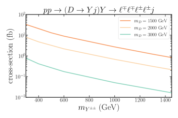
Figure 4: Cross section for the associated production of a bilepton with a VLQ. We consider the subsequent decay of the VLQ into a bilepton plus a quark, and the bilepton decay into electron or muon pairs.

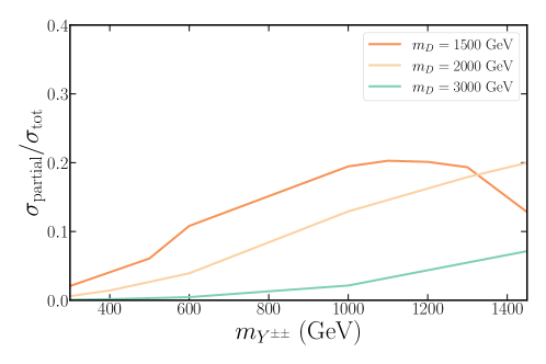
Figure 5: Ratio of the partial cross section for the bilepton associated production with a $D$ VLQ, which subsequently decays into a second bilepton, i.e. the $D$-$Y$ $\to YYj$ associated production ($\sigma_{\rm partial}$) over the total $YY+X$ cross section ($\sigma_{\rm tot}$).

Finally, another contribution to the inclusive bilepton pair production, which we have included in our study, come from the QCD pair production of extra VLQs, which both decay into a bilepton plus a jet: $pp\to({\rm VLQ}\to Y\,q)\;({\rm VLQ}\to Yq)\to YYjj$, with VLQ=$D,T$ and $j=u,b$, see Figure 6.

Figure 6: QCD pair production of VLQs, leading to a $YYjj$ final state.

4 Bilepton pair production at LHC

Given the phenomenological considerations expressed in the previous section, we find particularly promising the search for bileptons at the LHC. We want to focus in particular on the inclusive process $pp\to\ell^{\pm}\ell^{\pm}\ell^{\mp}\ell^{\mp}$, where a pair of $Y$ is produced on-shell and then decay to same sign leptons, allowing the presence of extra jets in the final state. We observe that ${\rm Br}(Y^{\pm\pm}\to\ell^{\pm}\ell^{\pm})\simeq 1$ because this is the only decay channel at tree level with our mass choice. Our analysis consistently considers all possible contributions to the inclusive bilepton pair production, and includes the processes whose diagrams are shown in Figures 1, 3, 6. For our analysis, we have implemented, by means of Feynrules Alloul et al. (2014), the 331 model we are considering ($A[\sqrt{3}]$) in a Universal Feynrules Output model Degrande et al. (2012), which we use for simulations and numeric calculations in MadGraph5 Alwall et al. (2014).

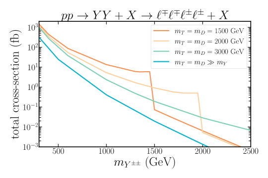
Figure 7: Inclusive cross section for the process $pp\to\ell^{\pm}\ell^{\pm}\ell^{\mp}\ell^{\mp}+X$ as function of the Y mass and for different values of the VLQ masses, and in the case of decoupled VLQ.

In Figure 7 we provide the inclusive cross section for the process $pp\to\ell^{\pm}\ell^{\pm}\ell^{\mp}\ell^{\mp}+X$ as function of the $Y$ mass and for different values of the VLQs masses, and in the case of decoupled VLQs. It is evident that processes involving VLQs which decay into bileptons constitute the dominant contribution to the bilepton pair inclusive cross section. Indeed, a large boost in the cross section, which reaches up to about two orders of magnitude near the kinematic threshold $m_{VLQ}\simeq m_{Y}$, is observed when the $VLQ\to Yq$ decays are on-shell. When these decays become off-shell, the cross section reduces significantly, despite a residual contribution from VLQ exchanged in the t-channel is still relevant.

A recent ATLAS search for doubly charged Higgs bosons, at the 13 TeV LHC with 139 fb^-1, focus on multilepton final states with at least one same-sign lepton pair Aad et al. (2023c). This analysis is therefore sensitive also to the bilepton pair production. We apply a recast of this analysis to extract a lower limit on the $Y$ mass.

4.1 Reinterpretation of the ATLAS search for doubly charged Higgs bosons

We summarize in the following paragraphs the main selection criteria considered in the ATLAS analysis Aad et al. (2023c), also adopting their notation. The search considers a final state with two (SR2L), three (SR3L) or four (SR4L) leptons, either electrons or muons, passing triggering requirements. The leptons must satisfy the transverse momentum $p_{T}$ and rapidity $\eta$ requirements: $p_{T}>$ 40 GeV and $|\eta_{\mu}|<$2.5, $|\eta_{e}|<$2.47 (for the electron, the region 1.37$<|\eta_{e}|<$1.52 is vetoed). Electron candidates are discarded if their angular distance $\Delta R=\sqrt{\Delta\phi^{2}+\Delta\eta^{2}}$ from a jet (with $p_{T}>$20 GeV and $|\eta|<$2.5) satisfies 0.2$<\Delta R<$0.4. If a muon and a jet featuring more than three tracks have a separation $\Delta R<$0.4 and the muon’s $p_{T}$ is less than half of the jet’s $p_{T}$, the muon is discarded. Signal regions are optimised to search for one same-charge lepton pair, in the case of two or three leptons, while four-lepton events are required to feature two same-charge pairs. The signal selection exploits, as the main variable to distinguish signal events from the background, the invariant mass of the two same-charge leptons with the highest $p_{T}$ in the event, $m(\ell^{\pm},\ell^{\prime\pm})_{\rm lead}$, and applies a cut:

$$m(\ell^{\pm},\ell^{\prime\pm})_{\rm lead}\geq 300\;{\rm GeV}\;.$$ (21)

Furthermore, for SR2L and SR3L, the vector sum of the two leading leptons’ transverse momenta must exceed 300 GeV:

$$p_{T}(\ell^{\pm},\ell^{\prime\pm})_{\rm lead}\geq 300\;{\rm GeV}\;\;{\rm(SR2L,SR3L)}$$ (22)

while, for SR4L, the average invariant mass of the two same-charge lepton pairs must satisfy:

$$\bar{m}=(m_{\ell^{+}\ell^{\prime+}}+m_{\ell^{-}\ell^{\prime-}})/2\geq 300\;{\rm GeV}\;\;{\rm(SR4L)}.$$ (23)

On top of these cuts, for SR3L and SR4L, a $Z$-veto condition is required, excluding the presence of same-charge lepton pairs with invariant mass 71 GeV$<m(\ell,\ell^{\prime})<$111.2 GeV. For SR2L, the requirement on the separation $\Delta R(\ell^{\pm},\ell^{\prime\pm})_{\rm lead}<3.5$ is considered. Finally, events containing jets identified as originating from b-quarks are vetoed.

We apply the above selection to the signal of inclusive bilepton pair production. Events are generated with Madgraph5 and then passed to Pythia8 Sjöstrand et al. (2015) for showering and hadronization. Jets are clustered by using Fastjet Cacciari et al. (2012) with an anti-kt algorithm with radius parameter $R=0.4$. Conservatively, based on the details of lepton reconstruction procedures described in Aad et al. (2023c), we also consider the following identification efficiencies for an electron: 0.58, and for a muon: 0.95.

We obtain the overall signal efficiencies reported in Table 2 for several signal benchmark points (we also list the values for the separate efficiencies in the SR4L and SR2L regions). The b-veto applied in the ATLAS analysis completely suppresses the contribution from the VLQ T to the bilepton pair production.

$m_{Y}$ (GeV)	300	600	1000	1300
$m_{D}$=1.5 TeV	0.14 ${}^{0.16}_{0.11}$	0.37 ${}^{0.37}_{0.11}$	0.36 ${}^{0.36}_{0.07}$	0.33 ${}^{0.32}_{0.11}$
$m_{D}$=2.0 TeV	0.14 ${}^{0.13}_{0.10}$	0.38 ${}^{0.37}_{0.08}$	0.38 ${}^{0.37}_{0.07}$	0.37 ${}^{0.36}_{0.14}$
$m_{D}$=3.0 TeV	0.13 ${}^{0.13}_{0.07}$	0.38 ${}^{0.38}_{0.10}$	0.38 ${}^{0.37}_{0.09}$	0.39 ${}^{0.38}_{0.08}$
$m_{D}\gg m_{Y}$	0.13 ${}^{0.13}_{0.06}$	0.38 ${}^{0.38}_{0.09}$	0.38 ${}^{0.37}_{0.09}$	0.39 ${}^{0.38}_{0.08}$

Table 2: Efficiencies of the inclusive bilepton pair production to the ATLAS selection Aad et al. (2023c) for several benchmark points of the minimal 331 model ($A[\sqrt{3}]$). We report the combined efficiencies for all of the three signal regions considered in the analysis, together with the specific efficiencies for the signal regions SR4L (upper values) and SR2L (lower values). The efficiencies for SR3L are similar to those obtained for SR4L.

For all of the benchmark points analyzed, except the lowest mass point, we find efficiencies for the bilepton pair process ($\epsilon_{YY}$) which are comparable to those for doubly-charged Higgs bosons ($\epsilon_{HH}$) in the SR3L and in the SR4L regions. For the SR2L region, we find in general slightly lower efficiencies than those obtained for the charged Higgs signal. In order to correctly compare the cross section for our process $pp\to YY\to\ell^{\pm}\ell^{\pm}\ell^{\mp}\ell^{\mp}$ with the upper limit band on the multi-lepton cross section reported in Fig. 8 of the ATLAS search Aad et al. (2023c), we consider a scaling of our cross section values by a factor $\epsilon_{YY}/\epsilon_{HH}$. Conservatively, the scaling is not applied when this factor is greater than 1. We show the result of the comparison in Fig. 8. We find that in the full mass region covered by the ATLAS analysis, and for all of the considered values of the mass of extra VLQs, the cross section for the process of inclusive bilepton pair production lies above the curve representing the 90% C.L. upper limit, with the lowest values obtained for the scenario of decoupled VLQs. We can therefore extract, independently of VLQ masses, the 90% C.L. bound on the bilepton mass:

$$m_{Y}>1300\;{\rm GeV}$$ (24)

This value supersedes the one obtained in Nepomuceno and Meirose (2020), $m_{Y}>1200$ GeV, which was based on the results of a previous ATLAS search for doubly charged Higgs bosons in multi-lepton final states with 36.1 fb^-1 at the 13 TeV LHC Aaboud et al. (2018b). It is clear from Fig. 8 that the search, with the increasing of the luminosity expected at the High-Luminosity LHC phase, has a great potential to test even larger bilepton (and VLQs) mass values, especially when the intertwined contribution of VLQs is taken into account.

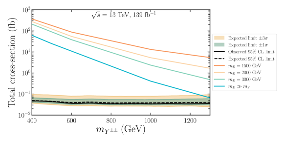
Figure 8: Alongside our prediction for the multi-lepton cross section generated by the bilepton pair production in the minimal 331 model, we illustrate the results obtained by ATLAS in Ref. Aad et al. (2023c). In particular, the solid and dashed lines represent the observed and expected 90% CL upper limits on the multi-lepton cross section as a function of the bilepton mass (doubly charged Higgs in the ATLAS analysis). The shaded green and yellow bands represent the $1\sigma$ and $3\sigma$ uncertainty around the combined expected limit.

5 Conclusions

We have considered a class of models, known as 331 models, characterized by the electroweak gauge group $SU_{L}(3)\times U(1)$. We have selected a minimal 331 model satisfying four general requests: 1) all matter multiplets include SM fermions, namely there are not multiplets including only BSM fermions; 2) all gauge bosons have integer charges; 3) all right-handed fermions are $SU(3)_{L}$ singlet and possess a left-handed counterpart 4) no gauge anomalies. These assumptions constrain the number of families: one possibility, although not the only one, is that it is a multiple of the color number. The model we have chosen has $\beta=\sqrt{3}$, the first two generations of quarks that transform as triplets under $SU_{L}(3)$, and the third generation of quark, together with the three lepton generations, that transform as anti-triplets. In addition to the usual SM fields, this model accommodates some BSM fields, namely three VLQs, $D^{1,2}$ and $T$, one neutral gauge boson $Z^{\prime}_{\mu}$, the charged boson $V^{\pm}_{\mu}$, and the doubly-charged bilepton $Y^{\pm\pm}_{\mu}$. The intertwined phenomenology of bileptons and VLQs looks particularly promising for the search and characterization of 331 models at the LHC. In our analysis, we propose bilepton pair signatures for 331 models, which are also efficient as search channels for VLQs. In particular, we focus on the inclusive production of a pair of doubly charged bileptons, followed by the decay of each bilepton into a pair of same-sign charged leptons, that is the process $pp\to Y^{++}Y^{--}\to\ell^{+}\ell^{+}\,\ell^{-}\ell^{-}+{\rm X}$. The final state of this inclusive process has multi-leptons (with at least one same-sign lepton pair), and possibly extra jets.

In our analysis, we provide the values of the inclusive cross section for the process $pp\to\ell^{+}\ell^{+}\,\ell^{-}\ell^{-}+{\rm X}$, as function of the doubly charged bilepton mass. We include consistently the production of doubly charged bileptons from gluon interaction, involving VLQs. A highly massive VLQ can decay into a bilepton and a SM quark $q$, yielding a final state $Y^{++}Y^{--}q$ or $Y^{++}Y^{--}qq$, which contribute to the inclusive process under investigation. At the best of our knowledge, the production from gluon-quark interaction of a bilepton associated to a VLQ has not been taken into account in previous searches for inclusive or exclusive bilepton pair production. We find that instead this contribution is significant in a large portion of the model parameter space (up to $\sim 20\%$ of the total inclusive cross section for the bilepton pair production).

A recent ATLAS search for doubly-charged Higgs bosons focuses on multi-lepton final states with at least one same-sign lepton pair Aad et al. (2023c). We apply a recast of this analysis to extract a lower limit on the $Y$ mass. We found, independently of the VLQs masses, a 90% CL lower limit on the mass of the doubly charged bilepton:

$$m_{Y}>1.3\,\,\mathrm{TeV}.$$ (25)

This value supersedes the previous one of $m_{Y}>1.2$ TeV Nepomuceno and Meirose (2020), based on 2017 ATLAS results.

We conclude by remarking that the channel we have investigated remains relevant with the increase of luminosity expected during the High-Luminosity LHC phase, due to its potential to test quite large bilepton (and VLQs) mass values.

Appendix A Basic features of 331 models

In this appendix, we present in more detail the general features of the 331 models. We are using the same convention of Ref. Buras et al. (2013). We do not discuss $SU(3)_{C}$ which does not change with respect to the SM. The generators of the $SU(3)_{\text{L}}$ gauge group are indicated with $\hat{T}^{1},\cdots,\hat{T}^{8}$. The generators of the fundamental representation of $SU(3)_{L}$ are $T^{a}=\lambda^{a}/2$, where ${\lambda}^{i}$ are the eight Gell-Mann matrices. For the $\bar{3}$ representation, the generators are $-(T^{a})^{T}$. The normalisation of the generators is $\mathrm{Tr}[T^{i}\,T^{j}]=\delta^{ij}/2$, and ${\mathds{1}}=\mathrm{diag}(1,1,1)$ is the identity matrix in the fundamental space. It is common to define the $U(1)_{X}$ generator as $T^{9}={\mathds{1}}/\sqrt{6}$. With this normalization $\mathrm{Tr}[T^{9}\,T^{9}]=1/2$, similarly to the one of $SU(3)_{\text{L}}$ generators.
In analogy with the SM the electric charge is defined as the diagonal operator

$$\hat{\mathcal{Q}}=\hat{T}^{3}+\frac{\hat{Y}}{2}$$ (26)

where we identify the hypercharge operator ${\hat{Y}}$ as in Eq. (1)

$$\frac{\hat{Y}}{2}=\beta\hat{T}^{8}+X{\mathds{1}}$$ (27)

In the SM left handed fermions are assigned to doublets of $SU_{L}(2)$. Similarly in 331 models one assigns left handed fields to fundamental irreducible representations ($3$ or $\overline{3}$) of $SU_{L}(3)$. We indicate them generically with $3_{Q,\ell}$ and $\overline{3}_{Q,\ell}$, distinguishing between quark triplets and anti-triplets ($3_{Q}$ and $\overline{3}_{Q}$) and lepton ones ($3_{\ell}$ and $\overline{3}_{\ell}$). Thus, for a generic SM quark-doublet $(u_{L},d_{L})$ we set

$$3_{Q}=\begin{pmatrix}u_{L}\\ d_{L}\\ \psi_{L}\end{pmatrix}_{i},\qquad\overline{3}_{Q}=\begin{pmatrix}d_{L}\\ -u_{L}\\ \Psi_{L}\end{pmatrix}_{j}.$$ (28)

In a similar way for a generic SM lepton-doublet $(\nu_{L},\ell_{L})$ we set

$$3_{\ell}=\begin{pmatrix}\nu_{L}\\ \ell_{L}\\ \xi_{L}\end{pmatrix}_{k},\qquad\overline{3}_{\ell}=\begin{pmatrix}\ell_{L}\\ -\nu_{L}\\ \zeta_{L}\end{pmatrix}_{r}.$$ (29)

The field assigned to the third components of these triplets are the left handed component of a field beyond the SM, namely we have introduced new fields $\psi_{i},\Psi_{j},\xi_{k},\zeta_{r}$. The indexes $i,j,k,r$ refer to flavor.

The action of the charge operator $\hat{\mathcal{Q}}$ on $3$ and $\bar{3}$ representations is given by the eigenvalues of the eigenstates $|3_{Q,\ell}\rangle$, and $|\overline{3}_{Q,\ell}\rangle$ that we indicate, respectively, as $\mathcal{Q}[3_{Q,\ell}]$ and $\mathcal{Q}[\overline{3}_{Q,\ell}]$. We have

$$\mathcal{Q}[3_{Q,\ell}(\overline{3}_{Q,\ell})]=\left(\begin{array}[]{ccc}\pm\frac{1}{2}\pm\frac{\beta}{2\sqrt{3}}+X[3_{Q,\ell}(\overline{3}_{Q,\ell})]&0&0\\ 0&\mp\frac{1}{2}\pm\frac{\beta}{2\sqrt{3}}+X[3_{Q,\ell}(\overline{3}_{Q,\ell})]&0\\ 0&&\mp\frac{\beta}{\sqrt{3}}+X[3_{Q,\ell}(\overline{3}_{Q,\ell})]\\ \end{array}\right),$$ (30)

The upper (down) signs correspond to the $3$ ($\bar{3}$) representations. The $X$ values for $3_{Q,\ell}$, and $\overline{3}_{Q,\ell}$ states are indicated, respectively, as $X[3_{Q,\ell}]$ and $X[\overline{3}_{Q,\ell}]$. We will use a similar notation $X[f]$ and $X[\overline{f}]$ if, instead of referring to all fields in an entire multiplet, we refer to the specific field $f$.

The charges of the first two components of (28) and (29) must match the charges of the corresponding SM fields. This matching fixes uniquely the $X$ values for the fermions as functions of $\beta$. Let us consider the case of the quark triplet $3_{Q}$. If we match the up quark charge $1/2+\beta/(2\sqrt{3})+X[{3}_{Q}]=2/3$, we obtain $X[{3}_{Q}]=1/6-\beta/(2\sqrt{3})$. The correct down quark charge follows automatically, and it does not represent an independent constraint. In the same way we get $X[{3}_{\ell}]=-1/2-\beta/(2\sqrt{3})$ in the lepton sector.
Let us now consider the entries of the matrix (30) for the antitriplets. By repeating the same reasoning for the quark assignment in (28) we get $X[\overline{3}_{Q}]=1/6+\beta/(2\sqrt{3})$, whereas for the lepton one in (29) we obtain $X[\overline{3}_{\ell}]=-1/2+\beta/(2\sqrt{3})$. Negative values for $\beta$ can be related to the positive ones by taking the complex conjugate in the covariant derivative of each model, which in turn is equivalent to replace $3$ with $\bar{3}$ in the fermion content of each particular model.

The non-standard fields, $\psi_{i},\Psi_{j},\xi_{k},\zeta_{r}$, have the same $X$ values of the other members of the respective (anti)triplet, because of gauge invariance. Thus using eq.(30) we deduce their charges, $\mathcal{Q}[\psi_{L}]=1/6-\sqrt{3}/2\,\beta$, $\mathcal{Q}[\Psi_{L}]=1/6+\sqrt{3}/2\,\beta$, $\mathcal{Q}[\xi_{L}]=-1/2-\sqrt{3}/2\,\beta$ and $\mathcal{Q}[\zeta_{L}]=-1/2+\sqrt{3}/2\,\beta$.

As far as right handed fields are concerned we assume, in analogy to the SM, that they are assigned to singlet representations of $SU_{L}(3)$. Since the action of the charge operator $\hat{\mathcal{Q}}$ on the singlet is given by $\hat{\mathcal{Q}}|1\rangle=X\,|1\rangle$, the $X$ value of a right-handed field coincides with its charge. In our notation, given a left-handed fermion field $f_{L}$, belonging to a triplet or anti-triplet $SU_{L}(3)$ representation, we indicate with $f_{R}$ the corresponding right-handed field in the $SU_{L}(3)$ singlet representation. Let us observe that the presence of right-handed quark singlets is demanded for the model to be $SU(3)_{C}$ vector-like. Table (3) summarises the quantum numbers of the 331 fermions.

	$SU_{c}(3)$	$SU_{L}(3)$	$U_{X}(1)$		$SU_{c}(3)$	$SU_{L}(3)$	$U_{X}(1)$
$\left(\begin{array}[]{c}u_{L}\\ d_{L}\\ \psi_{L}\end{array}\right)_{i}$	$3$	$3$	$\frac{1}{6}-\frac{\beta}{2\sqrt{3}}$	$\left(\begin{array}[]{c}\nu_{L}\\ \ell_{L}\\ \xi_{L}\end{array}\right)_{i}$	$1$	$3$	$-\frac{1}{2}-\frac{\beta}{2\sqrt{3}}$
$\left(\begin{array}[]{c}d_{L}\\ -u_{L}\\ \Psi_{L}\end{array}\right)_{i}$	$3$	$\overline{3}$	$\frac{1}{6}+\frac{\beta}{2\sqrt{3}}$	$\left(\begin{array}[]{c}\ell_{L}\\ -\nu_{L}\\ \zeta_{L}\end{array}\right)_{i}$	$1$	$\overline{3}$	$-\frac{1}{2}+\frac{\beta}{2\sqrt{3}}$
$u_{R_{i}}$	$3$	$1$	$\frac{2}{3}$
$d_{R_{i}}$	$3$	$1$	$-\frac{1}{3}$	$\ell_{R_{i}}$	$1$	$1$	$-1$
$\psi_{R_{i}}$	$3$	$1$	$\frac{1}{6}-\frac{\sqrt{3}\beta}{2}$	$\xi_{R_{i}}$	$1$	$1$	$-\frac{1}{2}-\frac{\sqrt{3}\beta}{2}$
$\Psi_{R_{i}}$	$3$	$1$	$\frac{1}{6}+\frac{\sqrt{3}\beta}{2}$	$\zeta_{R_{i}}$	$1$	$1$	$-\frac{1}{2}+\frac{\sqrt{3}\beta}{2}$

Table 3: Assigned representations and $X$ values of matter fields in terms of the parameter $\beta$ for a generic $331$ model. The subscript $i$ is a generic generation index.

Let us now us consider the 331 gauge bosons. Differently from the standard models we have 8 $W^{a}_{\mu}$ bosons for $SU_{L}(3)$ and one ${B_{X}}_{\mu}$ boson for $U_{X}(1)$. The covariant derivative acting on field representations are

• triplet: $D_{\mu}=\partial_{\mu}-igW^{a}_{\mu}T^{a}-ig_{X}X{B_{X}}_{\mu}T^{9}$;

• antitriplet: $D_{\mu}=\partial_{\mu}+igW^{a}_{\mu}(T^{a})^{T}-ig_{X}X{B_{X}}_{\mu}T^{9}$;

• singlet: $D_{\mu}=\partial_{\mu}-ig_{X}X{B_{X}}_{\mu}T^{9}$;

where the $g$ and $g_{X}$ are gauge couplings and a sum over $a$ is understood.

We arrange the $SU(3)_{\text{L}}$ gauge bosons $W_{\mu}^{a}$ as

$$W_{\mu}=W_{\mu}^{a}T^{a}=\frac{1}{2}\begin{pmatrix}W_{\mu}^{3}+\frac{1}{\sqrt{3}}W_{\mu}^{8}&\sqrt{2}W_{\mu}^{+}&\sqrt{2}Y_{\mu}^{Q_{Y}}\\ \sqrt{2}W_{\mu}^{-}&-W_{\mu}^{3}+\frac{1}{\sqrt{3}}W_{\mu}^{8}&\sqrt{2}V_{\mu}^{Q_{V}}\\ \sqrt{2}Y_{\mu}^{-Q_{Y}}&\sqrt{2}V_{\mu}^{-Q_{V}}&-\frac{2}{\sqrt{3}}W_{\mu}^{8}\end{pmatrix}$$ (31)

where

$$W^{\pm}_{\mu} = \frac{1}{\sqrt{2}}(W^{1}_{\mu}\mp iW_{\mu}^{2})$$

$$V_{\mu}^{\pm Q_{V}} = \frac{1}{\sqrt{2}}(W^{6}_{\mu}\mp iW_{\mu}^{7})$$ (32)

$$Y_{\mu}^{\pm Q_{Y}} = \frac{1}{\sqrt{2}}(W^{4}_{\mu}\mp iW_{\mu}^{5})$$

The action of the charge operator $\hat{\mathcal{Q}}$ on gauge bosons is given by the commutator $\left[\hat{\mathcal{Q}},W_{\mu}\right]$, and it can be represented by the matrix

$$\mathcal{Q}^{\rm GB}=\left(\begin{array}[]{ccc}0&1&\frac{1}{2}+\beta\frac{\sqrt{3}}{2}\\ -1&0&-\frac{1}{2}+\beta\frac{\sqrt{3}}{2}\\ -\frac{1}{2}-\beta\frac{\sqrt{3}}{2}&\frac{1}{2}-\beta\frac{\sqrt{3}}{2}&0\end{array}\right)$$ (33)

where each entry represents the charge of the gauge boson in the corresponding entry of the matrix 31. From eq.(33) we see that there are:

1. three neutral gauge bosons, $W^{3}_{\mu}$, $W^{8}_{\mu}$ and ${B_{X}}_{\mu}$. After the spontaneous symmetry breakings, the neutral gauge bosons mix originating three mass eigenstates, the SM $\gamma$ and $Z^{0}$ plus an additional neutral BSM gauge boson, generally indicated with $Z^{\prime}$;

2. two bosons with unit charges, corresponding to $W^{\pm}$;

3. four BSM bosons $Y_{\mu}^{\pm Q_{Y}},V_{\mu}^{\pm Q_{V}}$, with charges $\pm\mathcal{Q}_{Y}=\pm\frac{1}{2}\pm\beta\frac{\sqrt{3}}{2}$ and $\pm\mathcal{Q}_{V}=\mp\frac{1}{2}\pm\beta\frac{\sqrt{3}}{2}$, that depend on the value of $\beta$.

It is useful at this point to summarize the electric charges of BSM fermions and BSM bosons:

field	$\psi$	$\Psi$	$\xi$	$\zeta$	$\quad Z^{\prime}\quad$	$V$	$Y$
$\mathcal{Q}$	$\frac{1}{6}-\frac{\sqrt{3}}{2}\beta$	$\frac{1}{6}+\frac{\sqrt{3}}{2}\beta$	$-\frac{1}{2}-\frac{\sqrt{3}}{2}\beta$	$-\frac{1}{2}+\frac{\sqrt{3}}{2}\beta$	0	$\mp\frac{1}{2}\pm\frac{\sqrt{3}}{2}\beta$	$\pm\frac{1}{2}\pm\frac{\sqrt{3}}{2}\beta$

Depending on the choice of the parameter $\beta$ the electric charges of the new fields can be exotic. With exotic we mean charges different from $\pm 1/3,\pm 2/3$ for extra quarks, and different from $\pm 1$ for extra leptons and gauge bosons. We consider as a minimal requirement that the new gauge bosons have at least integer charge values, even if there are 331 models that discard this assumption, see for instance Romero Abad and Ramirez Barreto (2020).

By imposing that the new gauge bosons $Y_{\mu}^{\pm\mathcal{Q}_{Y}}$ and $V_{\mu}^{\pm\mathcal{Q}_{V}}$ have integer charge, it follows that the allowed values for the parameter $\beta$ are

$$\beta=\pm\frac{2n+1}{\sqrt{3}}\equiv\frac{r}{\sqrt{3}}$$ (34)

where $r$ is an odd integer number (positive or negative). A few examples of $X$ and $\hat{\mathcal{Q}}$ charges for new fields are reported in Table (4), corresponding to $r=\pm 1,\pm 3,\pm 5$. We immediately see that only the choice $r=\pm 1$ guarantees no exotic charges. It is necessary to warn that another constraint ($|r|\leq 3$) comes from spontaneous symmetry breaking, as we will see in sect. 2.2. In Table (4) we report the case $\beta=\pm 5/\sqrt{3}$ only to remark that in the minimal assumptions made up to now there is nothing that prevents $|r|$ from having values larger than $3$. From Table (4) it is also manifest that the exchange $r\longleftrightarrow-r$ is equivalent to trade triplets for anti-triplets and viceversa.

$r$	$+1$	$-1$	$+3$	$-3$	$+5$	$-5$
$X[\psi]$	$0$	$1/3$	$-1/3$	$2/3$	$-2/3$	$1$
$X[\Psi]$	$1/3$	$0$	$2/3$	$-1/3$	$1$	$-2/3$
$X[\xi]$	$-2/3$	$-1/3$	$-1$	$0$	$-4/3$	$1/3$
$X(\zeta)$	$-1/3$	$-2/3$	$0$	$-1$	$1/3$	$-4/3$
$\mathcal{Q}[\psi]$	$-1/3$	$2/3$	$-4/3$	$5/3$	$-7/3$	$8/3$
$\mathcal{Q}[\Psi]$	$2/3$	$-1/3$	$5/3$	$-4/3$	$8/3$	$-7/3$
$\mathcal{Q}[\xi]$	$-1$	$0$	$-2$	$1$	$-3$	$2$
$\mathcal{Q}[\zeta]$	$0$	$-1$	$1$	$-2$	$2$	$-3$
$|\mathcal{Q}[V]|$	$0$	$1$	$1$	$2$	$2$	$3$
$|\mathcal{Q}[Y]|$	$1$	$0$	$2$	$1$	$3$	$2$

Table 4: We list the $X$ values and the charges for the third components of quark triplet $3_{Q}$, lepton triplet $3_{\ell}$, quark anti-triplet $\overline{3}_{Q}$, lepton anti-triplet $\overline{3}_{\ell}$, and the absolute values of the charges of BSM gauge bosons for sample values of $r$ ($\beta=r/\sqrt{3}$).

The 331 models are fully characterized by the choice of the electric charge embedding, namely the pair $(\beta,X)$, of its fermionic content and multiplet assignemnts, and of the scalar sector. There are two major quantum field theory constraints, the absence of gauge anomalies and the possibility of QCD asymptotic freedom.

The fermionic structure is restricted by requiring the cancellation of the triangular anomalies. Both $SU(3)_{L}$ and $U(1)_{X}$ are anomalous, contrary to the SM, where only $U(1)_{Y}$ is. In the SM, gauge anomalies are cancelled out for every fermion family. This property is lost in 331 models and correlation between families is needed. Ref. Diaz et al. (2005) discusses in detail this topic for an arbitrary value of $\beta$ and number of generations. Below, we outline anomaly cancellation calculations assuming $N_{Q(\ell)}^{(3)}$ and $N_{Q(\ell)}^{(\overline{3})}$ quark (lepton) generations transforming as triplets and anti-triplets with the structure outlined above. We underline that when we refer to lepton generations, we mean generations of active leptons, whose left-handed parts are embedded in triplets or antitriplets. We define the total number of quark (lepton) generations as

$$N_{Q(\ell)}^{F}=N_{Q(\ell)}^{(3)}+N_{Q(\ell)}^{(\overline{3})}$$ (35)

The anomaly cancellations with their implications read as

• $[SU(3)_{L}]^{3}:$
  

  $N_{c}N_{Q}^{(3)}-N_{c}N_{Q}^{(\overline{3})}+N_{\ell}^{(3)}-N_{\ell}^{(\overline{3})}=0$
  

  $\Rightarrow N_{Q}^{(3)}=\frac{N_{c}N_{Q}^{F}+N_{\ell}^{F}}{2N_{c}}-\frac{N_{\ell}^{(3)}}{N_{c}}$

• $[SU(3)_{L}]^{2}\otimes U(1)_{X}$:
  

  $3N_{c}\left[N_{Q}^{(3)}X[3_{Q}]+N_{Q}^{(\overline{3})}X[\overline{3}_{Q}]\right]+3N_{\ell}^{(3)}X[3_{\ell}]+3N_{\ell}^{(\overline{3})}X[\overline{3}_{\ell}]=0$
  

  $\Rightarrow N_{Q}^{F}=\frac{3}{N_{c}}N_{\ell}^{F}$    (assuming A1))

• $[U(1)_{X}]^{3}$
  

  $N_{c}\left[N_{Q}^{(3)}\left(3X[3_{Q}]^{3}-X[\psi_{R}]^{3}\right)+N_{Q}^{(\overline{3})}\left(3X[\overline{3}_{Q}]^{3}-X[\Psi_{R}]^{3}\right)-N_{Q}^{F}\left(X[u_{R}]^{3}+X[d_{R}]^{3}\right)\right]+$
  $+N_{\ell}^{(3)}\left(3X[3_{\ell}]^{3}-X[\xi_{R}]^{3}\right)+N_{\ell}^{(\overline{3})}\left(3X[\overline{3}_{\ell}]^{3}-X[\zeta_{R}]^{3}\right)-N_{\ell}^{F}X[\ell_{R}]^{3}=0$
  

  $\Rightarrow$ No condition (always true).
  

• $[SU(3)_{c}]^{2}\otimes U(1)_{X}:$
  

  $N_{c}\left[N_{Q}^{(3)}\left(3X[3_{Q}]-X[\psi_{R}]\right)+N_{Q}^{(\overline{3})}\left(3X[\overline{3}_{Q}]-X[\Psi_{R}]\right)-N_{Q}^{F}\left(X[u_{R}]+X[d_{R}]\right)\right]=0$
  

  $\Rightarrow$ No condition (always true).
  

• $[\text{Grav}]^{2}\otimes U(1)_{X}$
  

  $N_{c}\left[N_{Q}^{(3)}\left(3X[3_{Q}]-X[\psi_{R}]\right)+N_{Q}^{(\overline{3})}\left(3X[\overline{3}_{Q}]-X[\Psi_{R}]\right)-N_{Q}^{F}\left(X[u_{R}]+X[d_{R}]\right)\right]+$
  $+N_{\ell}^{(3)}\left(3X[3_{\ell}]-X[\xi_{R}]\right)+N_{\ell}^{(\overline{3})}\left(3X[\overline{3}_{\ell}]-X[\zeta_{R}]\right)-N_{\ell}^{F}X[\ell_{R}]=0$
  

  $\Rightarrow$ No condition (always true).

where $N_{c}$ refers to the color $SU_{3}(N_{c})$, always fixed to $N_{c}=3$. The minus signs in the sum are due to the different fields chirality. We remark that these relations hold even under the common assumption $\zeta_{L}^{a}=(\ell^{a}_{R})^{c}$.

Before drawing conclusions from the anomaly cancellation, let us summarize the assumptions we have done on an otherwise completely general 331 model:

• all matter multiplets include SM fermions, excluding the possibility of fermion multiplets including only BSM fields;

• all gauge bosons, including BSM ones, have integer charges;

• all right-handed, $SU(3)$ singlet, fermions have a left-handed counterpart.

We underline that we could have assumed the presence of additional sterile right-handed or left-handed neutrinos in an arbitrary number without changing the above A1)-A7) conditions. Nor it would have changed the definition of $N^{F}_{Q(\ell)}$, which refers to weak interacting fermions.

We found from relation A2)

$$N_{\ell}^{F} = N_{Q}^{F}\equiv N_{F}\,,$$ (36)

namely the number of quark and charged lepton families must be the same. Combining A1) with A2) it follows

$$N_{Q}^{(3)} = \frac{1}{3}(2N_{F}-N_{\ell}^{(3)})\,.$$ (37)

Both sides of the equality must be integers. This is true if $N_{F}$ is a multiple of the color $N_{c}=3$, as in minimal models where $N_{\ell}^{(\bar{3})}=0$. However such proportionality is not strictly necessary. An example is $N_{F}=4$ with $N_{\ell}^{(3)}=N_{\ell}^{(\bar{3})}=2$ that gives $N_{Q}^{(3)}=N_{Q}^{(\bar{3})}=2$ (see also Ref. Diaz et al. (2005)).

Another constraints is given by $SU(3)_{c}$ asymptotic freedom. As in SM QCD, perturbative calculations limit the number of quark flavours to be equal to or less than 16. Since each family in 331 models has three flavours, that yields a constraint on the number of families: $N_{F}\leq 5$.

Summarizing, under the minimal assumptions discussed above, we can classify 331 models by means of $\beta=r/\sqrt{3}$, where $r=\pm 1,\pm 3$ (see for instance Pleitez (2021)), the family number $N_{F}\leq 5$, and the number of triplets or antitriplets for either quarks or leptons.

Fixing one of the 4 possible values for $\beta$, and assuming $N_{c}=N_{F}=3$, we have two possible choices, namely $N_{Q}^{3}=2,1$, that we name case A[$\beta$] and B[$\beta$], respectively. In Table 5 we report the numbers of quark and leptons in triplets and antitriplets according to the relations (35),(36) and (37). Note that this classification works only when triplet and anti-triplets are used, but it is also possible to assign matter fields to different representations like sextects, see for instance Ref. Fonseca and Hirsch (2016).

	$N_{Q}^{(3)}$	$N_{Q}^{(\bar{3})}$	$N_{\ell}^{(3)}$	$N_{\ell}^{(\bar{3})}$
A[$\beta$]	2	1	0	3
B[$\beta$]	1	2	3	0

Table 5: Number of triplets and anti-triplets in the lepton and quark sectors in case A[$\beta$] and B[$\beta$] (see text).

Models $A[\beta]$ and $B[-\beta]$ are related by the simultaneous exchange of fermion triplets $\to$ antitriplets and $\beta\to-\beta$. It implies that matter and gauge fields possess the same set of charges in both models . Several of these models have been discussed in literature: $A[1/\sqrt{3}]$  Montero et al. (1993); Buras et al. (2013); Boucenna et al. (2014), $A[-1/\sqrt{3}]$ Cabarcas et al. (2008); Profumo and Queiroz (2014); Cárcamo Hernández et al. (2016); Alves et al. (2022), $A[\sqrt{3}]$  Singer et al. (1980); Pisano and Pleitez (1992); Foot et al. (1993); Montero et al. (1999); Catano et al. (2012); Frampton (1992); Correia (2018); Corcella et al. (2018). The case A$[\sqrt{3}]$ is known as the minimal 331 model and will be considered in this work.

We remark that in order to fully specify a model fixing the matter content as above is not enough, but it has to be complemented by the assignment of the Higgs structures and vacuum alignments, see below.

Appendix B The model

2.1 The scalar sector

As mentioned in the introduction, the spontaneous symmetry breaking (SSB) pattern of 331 models occurs in two steps: the first one allows to recover the SM group structure, the second one is identifiable as the electroweak SSB. The 331 models are intrinsically multi-Higgs models, which, as in the SM, are $SU(3)_{C}$ singlets acquiring non-vanishing vacuum expectation values after SSB. They are responsible of mass terms for gauge bosons and fermions coupling to them. The requirement of gauge invariance of the Lagrangian term coupling one Higgs and two fermions constrains the Higgs representations. Namely, since the fermions $\psi$ transform either as a $3$ or as a $\bar{3}$ under $SU(3)_{L}$, we only have the following possibilities Diaz et al. (2004) for the Higgs field $\Phi$:

• $\bar{\psi}_{L}\psi_{R}\Phi$, with $\Phi\sim 3$;

• $\bar{\psi}_{L}(\psi_{L})^{c}\Phi$, with $\Phi\sim 6$;

• $\bar{\psi}_{R}(\psi_{R})^{c}\Phi$, with $\Phi\sim 1$;

• $\bar{\psi}_{L}(\psi^{\prime}_{L})^{c}\Phi$, with $\Phi\sim\bar{3}$;

The last possibility is allowed only if $\psi^{\prime}_{L}$ are completely exotic triplets with charged particles which are right handed charge-conjugated components Descotes-Genon et al. (2018), otherwise is zero. Singlets scalars are also scalars under $U(1)_{X}$ because of electromagnetic invariance. Thus, after the two steps of SSB, their vacuum expectation value will never give rise to a mass term for the gauge bosons or the charged fermions. Sextets are needed in some models, for instance to give Majorana masses to neutrinos as in Ref. Foot et al. (1993) or to allow a doubly-charged scalar to decay into same-sign leptons Corcella et al. (2018). Both singlets and sextets are not needed for the model and the phenomenology we are investigating, so we limit to the simpler, and widely used in literature, assumption of SSB by triplets only. The $X$ values of the triplets, and therefore also the charges of their components, are constrained by the requirement that the above Higgs-fermion coupling terms in the Lagrangian are also invariant under $U(1)_{X}$.

The Higgs triplets are:

$$\chi=\begin{pmatrix}\chi^{++}\\ \chi^{+}\\ \chi^{0}\end{pmatrix},\hskip 28.45274pt\rho=\begin{pmatrix}\rho^{+}\\ \rho^{0}\\ \rho^{-}\end{pmatrix},\,\hskip 28.45274pt\eta=\begin{pmatrix}\eta^{0}\\ \eta^{-}\\ \eta^{--}\end{pmatrix}.$$ (38)

Their $X$ values are listed in Table 1. The neutral components acquire a vacuum expectation value, namely $\langle\chi^{0}\rangle\equiv u$, $\langle\rho^{0}\rangle\equiv v$, $\langle\eta^{0}\rangle\equiv v^{\prime}$. In the first SSB, triggered by the triplet $\chi$, there are five gauge fields that acquire mass. In the second SSB, which requires the pair of triplets $\rho$ and $\eta$, three gauge fields acquire mass, leaving massless the field associated to the unbroken charge generator, that is the photon.

2.2 The gauge sector

Boson masses stem from the expansion of the covariant derivatives of the scalar sector

$$\mathcal{L}_{S}=(D_{\mu}\chi)(D^{\mu}\chi)^{\dagger}+(D_{\mu}\rho)(D^{\mu}\rho)^{\dagger}+(D_{\mu}\eta)(D^{\mu}\eta)^{\dagger}$$ (39)

The neutral gauge bosons matrix is not diagonal. In the base $W_{\mu}^{3},\,W_{\mu}^{8},\,B_{X\,\mu}$, it is given by

$$M_{0}=\frac{1}{4}\left(\begin{array}[]{ccc}g^{2}v^{2}_{+}&\frac{g^{2}}{\sqrt{3}}v_{-}^{2}&-\frac{gg_{X}}{3\sqrt{2}}\left(v_{+}^{2}\sqrt{3}-v_{-}^{2}\beta\right)\\ \frac{g^{2}}{\sqrt{3}}v_{-}^{2}&\frac{g^{2}}{3}\left(4u^{2}+v_{+}^{2}\right)&-\frac{gg_{X}}{9\sqrt{2}}\left(u^{2}4\sqrt{3}\beta+v_{+}^{2}\sqrt{3}\beta+3v_{-}^{2}\right)\\ -\frac{gg_{X}}{3\sqrt{2}}\left(v_{+}^{2}\sqrt{3}-v_{-}^{2}\beta\right)&-\frac{gg_{X}}{9\sqrt{2}}\left(u^{2}4\sqrt{3}\beta+v_{+}^{2}\sqrt{3}\beta+3v_{-}^{2}\right)&\frac{g_{X}^{2}}{18}\left(4u^{2}\beta^{2}+v_{+}^{2}(3+\beta^{2})+v_{-}^{2}2\sqrt{3}\right)\end{array}\right)$$ (40)

where $v^{2}_{-}=v^{\prime\,2}-v^{2}$.
Since $u^{2}\gg v_{+}^{2},\,v_{-}^{2}$ we can diagonalize this matrix in two steps. In the first one $B_{X\,\mu},\,W_{\mu}^{8}$ mix giving rise to $B^{\prime}_{\mu}$ and $Z^{\prime}_{\mu}$ as

$$\left(\begin{array}[]{c}W^{8}_{\mu}\\ B_{X\,\mu}\end{array}\right)\equiv\left(\begin{array}[]{cc}\cos\theta_{331}&-\sin\theta_{331}\\ \sin\theta_{331}&\cos\theta_{331}\\ \end{array}\right)\left(\begin{array}[]{c}B^{\prime}_{\mu}\\ Z^{\prime}_{\mu}\end{array}\right)\,.$$ (47)

With the above definition of the mixing angle, by diagonalizing $M_{0}$ we obtain

$$\sin\theta_{331}\simeq\frac{g}{\sqrt{g^{2}+g_{X}^{2}\beta^{2}/6}}\,.$$ (48)

Then at the second step $B^{\prime}_{\mu},Z_{\mu}^{\prime}$ mix both with $W_{\mu}^{3}$ but the mixing between $Z_{\mu}^{\prime}$ and $W_{\mu}^{3}$ is small compared to the one between $B^{\prime}_{\mu}$ and $W_{\mu}^{3}$, therefore the first one can be neglected and we have

$$\left(\begin{array}[]{c}W_{\mu}^{3}\\ B^{\prime}_{X\,\mu}\end{array}\right)\equiv\left(\begin{array}[]{cc}\cos\theta_{W}&\sin\theta_{W}\\ -\sin\theta_{W}&\cos\theta_{W}\\ \end{array}\right)\left(\begin{array}[]{c}Z_{\mu}\\ A_{\mu}\end{array}\right)$$ (55)

where $A_{\mu}$ is the Standard Model photon field. The corresponding boson masses are

$$m_{A} = 0\,,$$ (56)

$$m_{Z}^{2} \simeq \frac{g^{2}}{4\cos^{2}\theta_{W}}v_{\rm SM}^{2}\,$$ (57)

$$m_{Z^{\prime}}^{2} \simeq \frac{g^{2}u^{2}\cos^{2}\theta_{W}}{3[1-(1+\beta^{2})\sin^{2}\theta_{W}]}\,.$$ (58)

We note that $m_{W}^{2}/m_{Z}^{2}=\cos^{2}\theta_{W}$ and therefore we can identify $\theta_{W}$ with the Weinberg angle.

An important constraint for 331 models is obtained by imposing a matching condition for the coupling of $Z$ boson with fermions. In particular, considering the right-handed leptons $\ell_{R}$ with $X$-charge $X[\ell_{R}]=-1$, the covariant derivative is given by

$$D_{\mu}\ell_{R}=\partial_{\mu}\ell_{R}+ig_{X}\frac{B_{X_{\mu}}}{\sqrt{6}}\,\ell_{R}$$ (59)

From Eqs. (47) and (55) we have that

$$B_{X_{\mu}}=\cos\theta_{331}\,Z^{\prime}_{\mu}-\sin\theta_{331}\sin\theta_{W}Z_{\mu}+\sin\theta_{331}\cos\theta_{W}A_{\mu}$$ (60)

Then by singling out the coupling with $Z$ boson and by matching with the corresponding Standard Model coupling $g\sin^{2}\theta_{W}/\cos\theta_{W}$ we get

$$\frac{g_{X}}{g}=\frac{\sqrt{6}\sin\theta_{W}}{\cos\theta_{W}\sin\theta_{331}}=\frac{\sqrt{6}\sin\theta_{W}}{\sqrt{1-\sin^{2}\theta_{W}(1+\beta^{2})}}$$ (61)

where we have used eq. (48). Beyond tree level, the precise definition of $\sin^{2}\theta_{W}$ is renormalization scheme and energy dependent. Extending the tree-level formula $m_{W}^{2}/m_{Z}^{2}=\cos^{2}\theta_{W}$ to all orders of perturbation theory results in the on-shell value of $\sin^{2}\theta_{W}$ Sirlin (1980). Another widely used convention is the modified minimal subtraction ($\overline{\mathrm{MS}}$) scheme. We can see that the tree level Eq. (61) exhibits a Landau pole when $\sin^{2}\theta_{W}=1/(1+\beta^{2})$. As in other non asymptotically free theories, at the Landau pole the coupling constant $g_{X}$ becomes infinite. The energy scale of the Landau pole depends on the running of $\sin^{2}\theta_{W}$, which in turn depends on the matter content of the model. Besides, in the on-shell scheme, radiative corrections for $\sin^{2}\theta_{W}$ include $m_{t}^{2}$-dependent terms which can cause large corrections in higher orders. $\sin^{2}\theta_{W}$ depends not only on the gauge couplings, but also on the spontaneous symmetry breaking. In the SM framework, using the $\overline{\mathrm{MS}}$ scheme, it has been estimated that values of $\sin^{2}\theta_{W}$ around the upper limit of the constraint $\sin^{2}\theta_{W}<0.25$ do not arise before $\approx$ 4 TeV Amoroso et al. (2023). There are 1-loop analyses that estimate that at large values of the coupling, that is even before the Landau pole is reached, the model may lose its perturbative character Martinez and Ochoa (2007); Dias et al. (2005); Dias and Pleitez (2009); Dias et al. (2006) (see also the discussion in Buras et al. (2014)). At the same time, some of these analyses indicate how to push the non-perturbative regime, and the Landau pole, up to much higher scales, including for example heavy resonances as active degrees of freedom in the running Martinez and Ochoa (2007); Dias (2005). We stress anyway that the typical energy scale of bilepton-pair production we consider is of the order of $\approx 2\,m_{Y}\approx 2$ TeV. Given the considerations above, we assume that no significative barrier is posed by the Landau pole to the perturbative analysis carried out in the present study.

We also note that the left-hand side of eq. (61) is real if (see also Fonseca and Hirsch (2016))

$$|\beta|<\frac{\cos\theta_{W}}{\sin\theta_{W}}\simeq 1.83\,.$$ (62)

This upper limit of $|\beta|$ is extremely important for the model building. As shown above the only allowed values for $|\beta|$ are $r/\sqrt{3}$ with $r$ integer. The constraint coming from eq. (62) yields $n\leq 3$ and therefore models with $n>3$ are not allowed in this minimal framework.

Appendix C Decay rates and vertices

Here we report the decay widths of the VLQs introduced in the model:

$$\Gamma(T\to Y^{++}d^{a})=\frac{g^{2}|{{\cal V}_{L}}_{3a}|^{2}}{64\pi}\frac{m^{6}_{T}-3m^{2}_{T}m^{4}_{Y}+2m^{6}_{Y}}{m^{3}_{T}m^{2}_{Y}}\,,$$ (63)

$$\Gamma(D^{i}\to Y^{--}u^{a})=\frac{g^{2}|{{\cal U}_{L}}_{ia}|^{2}}{64\pi}\frac{m^{6}_{D}-3m^{2}_{D}m^{4}_{Y}+2m^{6}_{Y}}{m^{3}_{D}m^{2}_{Y}}\,,$$ (64)

$$\Gamma(T\to V^{+}u^{a})=\frac{g^{2}|{{\cal U}_{L}}_{3a}|^{2}}{64\pi}\frac{m^{6}_{T}-3m^{2}_{T}m^{4}_{V}+2m^{6}_{V}}{m^{3}_{T}m^{2}_{V}}\,,$$ (65)

$$\Gamma(D^{i}\to V^{-}d^{a})=\frac{g^{2}|{{\cal V}_{L}}_{ia}|^{2}}{64\pi}\frac{m^{6}_{D}-3m^{2}_{D}m^{4}_{V}+2m^{6}_{V}}{m^{3}_{D}m^{2}_{V}}\,,$$ (66)

where $m_{X}$ stays for the mass of the $X$ field. The bilepton $Y$ decay width is

$$\Gamma(Y\to\ell^{\pm}\ell^{\pm})=\frac{g^{2}}{12\pi}m_{Y}\,.$$ (67)

In the following tables we give the relevant vertices of the model:

Gauge boson-fermion interactions
Vertex	Coupling	Vertex	Coupling
$V$ boson		$Y$ boson
	$\frac{g}{\sqrt{2}}\mathcal{U}_{L\,3a}$		$-\frac{g}{\sqrt{2}}\mathcal{V}_{L\,3a}$
	$\frac{g}{\sqrt{2}}\mathcal{V}_{L\,ia}$		$\frac{g}{\sqrt{2}}\mathcal{U}_{L\,ia}$
	$\frac{g}{\sqrt{2}}$		$-\frac{g}{\sqrt{2}}$
$Z$ boson
	$\frac{g}{c_{w}}\left(\frac{1}{6}+\frac{\sqrt{3}}{2}\beta\right)s_{w}^{2}$		$\frac{g}{c_{w}}\left(-\frac{1}{6}+\frac{\sqrt{3}}{2}\beta\right)s_{w}^{2}$
	$\frac{g}{2c_{w}}\left(1-\sqrt{3}\beta\right)s_{w}^{2}$
$Z^{\prime}$ boson
	$\frac{g\left[1-(1+\sqrt{3}\beta)s_{w}^{2}\right]}{2\sqrt{3}c_{w}\sqrt{1-(1+\beta^{2})s_{w}^{2}}}$		$-\frac{g\beta s_{w}^{2}}{c_{w}\sqrt{1-(1+\beta^{2})s_{w}^{2}}}$
	$-\frac{g\left[2-\left(2-\sqrt{3}\beta(1-\sqrt{3}\beta)\right)s_{w}^{2}\right]}{2\sqrt{3}c_{w}\sqrt{1-(1+\beta^{2})s_{w}^{2}}}$		$-\frac{g(1-\sqrt{3}\beta)\beta s_{w}^{2}}{2c_{w}\sqrt{1-(1+\beta^{2})s_{w}^{2}}}$
	$\frac{g\left[[-1+(\beta/\sqrt{3})s_{w}^{2}]\delta_{ab}+2c_{w}^{2}\mathcal{U}^{*}_{L\,3a}\mathcal{U}_{L\,3b}\right]}{2\sqrt{3}c_{w}\sqrt{1-(1+\beta^{2})s_{w}^{2}}}$		$\frac{2g\beta s_{w}^{2}\delta_{ab}}{3c_{w}\sqrt{1-(1+\beta^{2})s_{w}^{2}}}$
	$\frac{g\left[[-1+(\beta/\sqrt{3})s_{w}^{2}]\delta_{ab}+2c_{w}^{2}\mathcal{V}^{*}_{L\,3a}\mathcal{V}_{L\,3b}\right]}{2\sqrt{3}c_{w}\sqrt{1-(1+\beta^{2})s_{w}^{2}}}$		$-\frac{g\beta s_{w}^{2}\delta_{ab}}{3c_{w}\sqrt{1-(1+\beta^{2})s_{w}^{2}}}$
	$\frac{g\left[2+\left(-2\sqrt{3}+\beta(1-3\sqrt{3}\beta)\right)s_{w}^{2}/\sqrt{3}\right]}{2\sqrt{3}c_{w}\sqrt{1-(1+\beta^{2})s_{w}^{2}}}$		$\frac{g\beta(1-3\sqrt{3}\beta)s_{w}^{2}}{6c_{w}\sqrt{1-(1+\beta^{2})s_{w}^{2}}}$
	$\frac{g\left[-2+\left(2\sqrt{3}+\beta(1-3\sqrt{3}\beta)\right)s_{w}^{2}/\sqrt{3}\right]}{2\sqrt{3}c_{w}\sqrt{1-(1+\beta^{2})s_{w}^{2}}}$		$\frac{g\beta(1+3\sqrt{3}\beta)s_{w}^{2}}{6c_{w}\sqrt{1-(1+\beta^{2})s_{w}^{2}}}$

References

- Ross (1985) G. G. Ross, Grand Unified Theories (1985).
- Langacker (2009) P. Langacker, Rev. Mod. Phys. 81, 1199 (2009), arXiv:0801.1345 [hep-ph] .
- Mohapatra and Pati (1975) R. N. Mohapatra and J. C. Pati, Phys. Rev. D 11, 566 (1975).
- Senjanovic and Mohapatra (1975) G. Senjanovic and R. N. Mohapatra, Phys. Rev. D 12, 1502 (1975).
- Schechter and Ueda (1973) J. Schechter and Y. Ueda, Phys. Rev. D 8, 484 (1973).
- Gupta and Mani (1974) V. Gupta and H. S. Mani, Phys. Rev. D 10, 1310 (1974).
- Albright et al. (1975) C. H. Albright, C. Jarlskog, and M. O. Tjia, Nucl. Phys. B 86, 535 (1975).
- Georgi and Pais (1979) H. Georgi and A. Pais, Phys. Rev. D 19, 2746 (1979).
- Glashow et al. (1970) S. L. Glashow, J. Iliopoulos, and L. Maiani, Phys. Rev. D 2, 1285 (1970).
- Singer et al. (1980) M. Singer, J. W. F. Valle, and J. Schechter, Phys. Rev. D 22, 738 (1980).
- Pisano and Pleitez (1992) F. Pisano and V. Pleitez, Phys. Rev. D 46, 410 (1992), arXiv:hep-ph/9206242 .
- Frampton (1992) P. H. Frampton, Phys. Rev. Lett. 69, 2889 (1992).
- Descotes-Genon et al. (2018) S. Descotes-Genon, M. Moscati, and G. Ricciardi, Phys. Rev. D 98, 115030 (2018), arXiv:1711.03101 [hep-ph] .
- Romero Abad and Ramirez Barreto (2020) D. Romero Abad and E. Ramirez Barreto, J. Phys. Conf. Ser. 1558, 012001 (2020).
- Fonseca and Hirsch (2016) R. M. Fonseca and M. Hirsch, JHEP 08, 003 (2016), arXiv:1606.01109 [hep-ph] .
- Diaz et al. (2005) R. A. Diaz, R. Martinez, and F. Ochoa, Phys. Rev. D 72, 035018 (2005), arXiv:hep-ph/0411263 .
- Corcella et al. (2018) G. Corcella, C. Corianò, A. Costantini, and P. H. Frampton, Phys. Lett. B 785, 73 (2018), arXiv:1806.04536 [hep-ph] .
- Amoroso et al. (2023) S. Amoroso, M. Chiesa, C. L. Del Pio, K. Lipka, F. Piccinini, F. Vazzoler, and A. Vicini, Phys. Lett. B 844, 138103 (2023), arXiv:2302.10782 [hep-ph] .
- Buras et al. (2013) A. J. Buras, F. De Fazio, J. Girrbach, and M. V. Carlucci, JHEP 02, 023 (2013), arXiv:1211.1237 [hep-ph] .
- Aad et al. (2015) G. Aad et al. (ATLAS), JHEP 08, 105 (2015), arXiv:1505.04306 [hep-ex] .
- Sirunyan et al. (2018) A. M. Sirunyan et al. (CMS), Phys. Lett. B 779, 82 (2018), arXiv:1710.01539 [hep-ex] .
- Aaboud et al. (2018a) M. Aaboud et al. (ATLAS), Phys. Rev. D 98, 112010 (2018a), arXiv:1806.10555 [hep-ex] .
- Aad et al. (2023a) G. Aad et al. (ATLAS), Phys. Lett. B 843, 138019 (2023a), arXiv:2210.15413 [hep-ex] .
- Aad et al. (2023b) G. Aad et al. (ATLAS), (2023b), arXiv:2305.03401 [hep-ex] .
- Corcella et al. (2021) G. Corcella, A. Costantini, M. Ghezzi, L. Panizzi, G. M. Pruna, and J. Šalko, JHEP 10, 108 (2021), arXiv:2107.07426 [hep-ph] .
- Sirunyan et al. (2019) A. M. Sirunyan et al. (CMS), JHEP 03, 082 (2019), arXiv:1810.03188 [hep-ex] .
- Oliveira and de S. Pires (2022) V. Oliveira and C. A. de S. Pires, Phys. Rev. D 106, 015031 (2022), arXiv:2112.03963 [hep-ph] .
- Alves et al. (2022) A. Alves, L. Duarte, S. Kovalenko, Y. M. Oviedo-Torres, F. S. Queiroz, and Y. S. Villamizar, Phys. Rev. D 106, 055027 (2022), arXiv:2203.02520 [hep-ph] .
- Addazi et al. (2022) A. Addazi, G. Ricciardi, S. Scarlatella, R. Srivastava, and J. W. F. Valle, Phys. Rev. D 106, 035030 (2022), arXiv:2201.12595 [hep-ph] .
- Alves et al. (2023) A. Alves, G. G. da Silveira, V. P. Gonçalves, F. S. Queiroz, Y. M. Oviedo-Torres, and J. Zamora-Saa, (2023), arXiv:2309.00681 [hep-ph] .
- Contino et al. (2007) R. Contino, T. Kramer, M. Son, and R. Sundrum, JHEP 05, 074 (2007), arXiv:hep-ph/0612180 .
- Vignaroli (2014) N. Vignaroli, Phys. Rev. D 89, 095027 (2014), arXiv:1404.5558 [hep-ph] .
- Vignaroli (2015) N. Vignaroli, Phys. Rev. D 91, 115009 (2015), arXiv:1504.01768 [hep-ph] .
- Bini et al. (2012) C. Bini, R. Contino, and N. Vignaroli, JHEP 01, 157 (2012), arXiv:1110.6058 [hep-ph] .
- Altarelli et al. (1989) G. Altarelli, B. Mele, and M. Ruiz-Altaba, Z. Phys. C 45, 109 (1989), [Erratum: Z.Phys.C 47, 676 (1990)].
- Mohan and Vignaroli (2015) K. Mohan and N. Vignaroli, JHEP 10, 031 (2015), arXiv:1507.03940 [hep-ph] .
- Dion et al. (1999) B. Dion, T. Gregoire, D. London, L. Marleau, and H. Nadeau, Phys. Rev. D 59, 075006 (1999), arXiv:hep-ph/9810534 .
- Corcella et al. (2017) G. Corcella, C. Coriano, A. Costantini, and P. H. Frampton, Phys. Lett. B 773, 544 (2017), arXiv:1707.01381 [hep-ph] .
- Nepomuceno and Meirose (2020) A. Nepomuceno and B. Meirose, Phys. Rev. D 101, 035017 (2020), arXiv:1911.12783 [hep-ph] .
- Dutta and Nandi (1994) B. Dutta and S. Nandi, Phys. Lett. B 340, 86 (1994).
- Alloul et al. (2014) A. Alloul, N. D. Christensen, C. Degrande, C. Duhr, and B. Fuks, Comput. Phys. Commun. 185, 2250 (2014), arXiv:1310.1921 [hep-ph] .
- Degrande et al. (2012) C. Degrande, C. Duhr, B. Fuks, D. Grellscheid, O. Mattelaer, and T. Reiter, Comput. Phys. Commun. 183, 1201 (2012), arXiv:1108.2040 [hep-ph] .
- Alwall et al. (2014) J. Alwall, R. Frederix, S. Frixione, V. Hirschi, F. Maltoni, O. Mattelaer, H. S. Shao, T. Stelzer, P. Torrielli, and M. Zaro, JHEP 07, 079 (2014), arXiv:1405.0301 [hep-ph] .
- Aad et al. (2023c) G. Aad et al. (ATLAS), Eur. Phys. J. C 83, 605 (2023c), arXiv:2211.07505 [hep-ex] .
- Sjöstrand et al. (2015) T. Sjöstrand, S. Ask, J. R. Christiansen, R. Corke, N. Desai, P. Ilten, S. Mrenna, S. Prestel, C. O. Rasmussen, and P. Z. Skands, Comput. Phys. Commun. 191, 159 (2015), arXiv:1410.3012 [hep-ph] .
- Cacciari et al. (2012) M. Cacciari, G. P. Salam, and G. Soyez, Eur. Phys. J. C 72, 1896 (2012), arXiv:1111.6097 [hep-ph] .
- Aaboud et al. (2018b) M. Aaboud et al. (ATLAS), Eur. Phys. J. C 78, 199 (2018b), arXiv:1710.09748 [hep-ex] .
- Pleitez (2021) V. Pleitez, in 5th Colombian Meeting on High Energy Physics (2021) arXiv:2112.10888 [hep-ph] .
- Hue and Ninh (2019) L. T. Hue and L. D. Ninh, Eur. Phys. J. C 79, 221 (2019), arXiv:1812.07225 [hep-ph] .
- Montero et al. (1993) J. C. Montero, F. Pisano, and V. Pleitez, Phys. Rev. D 47, 2918 (1993), arXiv:hep-ph/9212271 .
- Boucenna et al. (2014) S. M. Boucenna, S. Morisi, and J. W. F. Valle, Phys. Rev. D 90, 013005 (2014), arXiv:1405.2332 [hep-ph] .
- Cabarcas et al. (2008) J. M. Cabarcas, D. Gomez Dumm, and R. Martinez, Eur. Phys. J. C 58, 569 (2008), arXiv:0809.0821 [hep-ph] .
- Profumo and Queiroz (2014) S. Profumo and F. S. Queiroz, Eur. Phys. J. C 74, 2960 (2014), arXiv:1307.7802 [hep-ph] .
- Cárcamo Hernández et al. (2016) A. E. Cárcamo Hernández, R. Martinez, and F. Ochoa, Eur. Phys. J. C 76, 634 (2016), arXiv:1309.6567 [hep-ph] .
- Foot et al. (1993) R. Foot, O. F. Hernandez, F. Pisano, and V. Pleitez, Phys. Rev. D 47, 4158 (1993), arXiv:hep-ph/9207264 .
- Montero et al. (1999) J. C. Montero, V. Pleitez, and O. Ravinez, Phys. Rev. D 60, 076003 (1999), arXiv:hep-ph/9811280 .
- Catano et al. (2012) M. E. Catano, R. Martinez, and F. Ochoa, Phys. Rev. D 86, 073015 (2012), arXiv:1206.1966 [hep-ph] .
- Correia (2018) F. C. Correia, J. Phys. G 45, 043001 (2018), arXiv:1704.00786 [hep-ph] .
- Diaz et al. (2004) R. A. Diaz, R. Martinez, and F. Ochoa, Phys. Rev. D 69, 095009 (2004), arXiv:hep-ph/0309280 .
- Sirlin (1980) A. Sirlin, Phys. Rev. D 22, 971 (1980).
- Martinez and Ochoa (2007) R. Martinez and F. Ochoa, Eur. Phys. J. C 51, 701 (2007), arXiv:hep-ph/0606173 .
- Dias et al. (2005) A. G. Dias, R. Martinez, and V. Pleitez, Eur. Phys. J. C 39, 101 (2005), arXiv:hep-ph/0407141 .
- Dias and Pleitez (2009) A. G. Dias and V. Pleitez, Phys. Rev. D 80, 056007 (2009), arXiv:0908.2472 [hep-ph] .
- Dias et al. (2006) A. G. Dias, J. C. Montero, and V. Pleitez, Phys. Lett. B 637, 85 (2006), arXiv:hep-ph/0511084 .
- Buras et al. (2014) A. J. Buras, F. De Fazio, and J. Girrbach, JHEP 02, 112 (2014), arXiv:1311.6729 [hep-ph] .
- Dias (2005) A. G. Dias, Phys. Rev. D 71, 015009 (2005), arXiv:hep-ph/0412163 .