Mercury: a Modeling, Simulation, and Optimization Framework for Data Stream-Oriented IoT Applications

Abstract

The Internet of Things is transforming our society by monitoring users and infrastructures’ behavior to enable new services that will improve life quality and resource management. These applications require a vast amount of localized information to be processed in real-time so, the deployment of new fog computing infrastructures that bring computing closer to the data sources is a major concern. In this context, we present Mercury, a Modeling, Simulation, and Optimization (M&S&O) framework to analyze the dimensioning and the dynamic operation of real-time fog computing scenarios. Our research proposes a location-aware solution that supports data stream analytics applications including FaaS-based computation offloading. Mercury implements a detailed structural and behavioral simulation model, providing fine-grained simulation outputs, and is described using the Discrete Event System Specification (DEVS) mathematical formalism, helping to validate the model’s implementation. Finally, we present a case study using real traces from a driver assistance scenario, offering a detailed comparison with other state-of-the-art simulators.

1 Introduction

The escalating process of digitalization is triggering the proliferation of new Internet of Things (IoT) services and applications. The IoT technological revolution is transforming our society by recording and analyzing the behavior of users and infrastructures to develop services for improving quality of life and resource management. This technology is in full growth, and the deployment of tens of billions of devices connected to the internet is expected within the next few years [1].

Computing IoT-based environments need Big Data infrastructures for effective real-time decision making, capable of processing large amounts of complex data from multiple, geographically distributed sources. Moreover, many IoT applications demand low latencies and rapid mobility [2]. However, for Big Data when response time is critical, cloud computing is not capable of meeting these needs and traditional networks  would also impose overloads to the communication bandwidth of the core network [3].

Therefore, a new paradigm is emerging. Fog computing was introduced by researchers from Cisco Systems in 2012 [4]. It extends the cloud computing paradigm to the edge of the network, deploying micro data centers that operate on the edge and provides a drastic latency reduction compared to cloud computing [5]. These Edge Data Centers (EDCs) process information from heterogeneous IoT data sources, perform the operations that require the minimum response time, and aggregate the data for subsequent sending to the cloud, thus decongesting the communications network and avoiding its saturation [6]. Recent research reports that in this computing paradigm the Round-Trip Time (RTT) may be reduced by 92% and the overall available bandwidth may be increased by a factor of 47-58 when compared to a cloud platform [7].

Many relevant IoT applications can take advantage of these features, as i) those based on distributed monitoring systems using embedded devices with limited processing capacity (e.g., environmental analysis), and ii) real-time data stream analytics, processing a large volume of data (e.g., e-health and driving assistance systems) [8, 9].  However, the new edge infrastructure needed to support fog computing requires the deployment of numerous smaller data centers that can be relocated to bring computing closer to the origin of the information. Moreover, those data centers’ energy consumption must be within the margins supported by the electricity grid. To reduce the consumption of the edge infrastructure and improve its availability, the concept of an edge federation arises.

The federation of EDCs allows the combined management of both the resource demand depending on the volume of users, their physical location and the use of the available renewable energy sources, thus reducing the carbon footprint [10]. Also, this location-awareness particularities of fog computing make the  Function as a Service (FaaS)-based management of applications of great interest to further optimize resource utilization in the edge federation [11].

Moreover, IoT applications depict a pervasive network of multiple distributed wireless devices that are both resource and energy-limited, all able to collect and send large volumes of heterogeneous environmental information in real-time. Due to the energy-computing-bandwidth limitations of the wireless domain, the 5G mobile communication standard arises as a service enabler to overcome these technical barriers. 5G appears as a highly flexible technology that provides a solid field for IoT applications with diverse requirements deployment. Together with IoT and fog computing, 5G promises to cause a technology disruption in a wide range of business sectors.

Currently, IoT models and simulators are in great need, since the conception, design, implementation, and deployment of such complex architectures as edge federations, demand in-depth virtual analysis.  The nature of the problem suggests the application of solid advanced Modeling and Simulation (M&S) methods based on the principles of Model-Based Systems Engineering (MBSE) that ensures a logic, robust, and reliable incremental design. We capitalize on the principles of MBSE of evolving the model - defined using the Discrete Event System Specification (DEVS) formalism - as the central artifact throughout the lifecycle of the system.

In this context we present Mercury, a Modeling, Simulation, and Optimization (M&S&O) framework designed to explore the dimensioning and the dynamic operation of real-time fog computing scenarios. Mercury is open source, and it can be downloaded from its official repository [12]. Particularly, the contributions of our research are the following:

• Our model exploits the location-awareness inherent in fog computing by implementing a FaaS-based computation offloading over a network with 5G capabilities. Mercury supports data stream analytics applications, as they may obtain the most benefits from this scenario, as real-time low latency and high data volume throughput, avoiding network congestion.

• We provide a high-detailed structural and behavioral simulation model based on MBSE, where the DEVS mathematical formalism helps to validate the atomic models’ implementation.

• This approach allows Mercury to provide more detailed simulation outputs, including real-time data for heterogeneously configured IT and network resources. We also provide an allocation manager to automatically optimize the configuration of the model to be explored. This makes Mercury a powerful M&S&O framework to analyze both location-aware deployments and dynamic operation strategies for the edge infrastructure.

• In this paper, as a case study, we model a realistic Advanced Driver Assistance System (ADAS) application based on data stream analytics using real traces from traffic mobility and from vehicles’ onboard cameras. Also, we offer a detailed comparison with other state-of-the-art fog computing simulators to highlight Mercury’s novelties.

The present research paper is a significant extension of our previous research [13], in which we presented an edge federation M&S framework for data stream analytics focused on evaluating the power and delay perceived at the edge layer. In the present publication we significantly extend this approach to introduce Mercury. Following are the main contributions added to our previous research:

• Mercury now includes a detailed 5G-based model (e.g., radio interface, physical interface, bandwidth assignation schematics, signal encoding and bit rates) to increase the realism of the radio interfaces’ impact on fog computing. Hence, the new research presents a solution for a complete fog scenario instead of focusing only on the edge computing infrastructure.

• Mercury allows the user to monitor, not only power and delay, but also bandwidth share, spectral efficiency and bit rate at the radio interface side. Also, 2D Mobility is currently supported natively by Mercury.

• Our previous research provided an M&S tool, where the placement of network and computing infrastructures must be provided manually. Mercury is an M&S&O framework that also provides an allocation manager module for scenario optimizations, automatically determining the location of both the network and the computing infrastructures according to the IoT application under study.

• The present research has a completely novel performance evaluation. Mercury has been validated under a realistic scenario with further complexity, including real traces of IoT devices’ GPS location history. We provide an evaluation of power, delay, bandwidth share, spectral efficiency and bit rate outputs for the use-case scenario configurations under discussion. This paper also includes a detailed performance comparison with other state-of-the-art fog computing M&S frameworks.

The remainder of this paper is organized as follows: in Section 2, the state-of-the-art on simulation tools for fog computing environments is provided.  Sections 3 and 4 give further information on the architecture of Mercury and its implementation. Section 5 presents an ADAS use case scenario and extensively explains the performance evaluation and a comparison with other state-of-the-art alternatives.  Finally, in Section 6, the main conclusions and future directions are outlined.

2 State of the Art

This section presents several M&S tools that are extensively used for specific use cases that could benefit from edge and fog computing scenarios. These frameworks tend to focus on the potential benefits that fog computing could contribute to the service instead of the edge computing infrastructure itself. As an example, one widespread use case is ADAS. Research provided by He et al. [14] includes software for the recognition and location of traffic signals for driving assistance scenarios that make use of edge computing features. In this research, three main elements are identified: intelligent vehicles, edge servers, and cloud servers. The functionality of each of them is detailed, as well as their interactions. However, communication, power consumption, and latency analysis are not explained in detail. Yuan et al. [15] present a content caching strategy for driving assistance applications in which the content delivery is edge-assisted, and both Vehicle-to-Vehicle (V2V) and Vehicle-to-Infrastructure (V2I) communications are extensively used for enhancing driving assistance functions. They also present the prediction of the service content demand in a delay-constrained scenario. Moreover, Li et al. [16] provide an IoT scenario that includes both edge and cloud infrastructures for ADAS data stream applications. Their research presents power models and analysis for both Long Term Evolution (LTE) network and IoT devices, but the latency analysis is not explained in detail.

Even though the previous ADAS-based research works introduce important aspects for service-specific purposes, they provide neither power consumption nor resource management of the edge data centers’ layer. The 5G model is not included in any of these research works as well.

On the other hand, there are fog computing frameworks that focus on the required infrastructure for providing fog services, regardless of the IoT application. These frameworks usually focus on infrastructure design parameters and are intended to be used for fog computing infrastructure dimensioning and management. EdgeCloudSim [17] presents a framework for the performance evaluation of edge architectures. Their network model includes Metropolitan Area Networks (MANs), Wide Area Networks (WANs), and Wireless Local Area Networks (WLANs), but they do not provide the power consumption analysis in the infrastructure. Gupta et al. [18] present the iFogSim simulator for modeling and simulation of the resource management of both fog and edge scenarios. Their research does not include location capabilities, but its development would be included in their future directions. However, none of these edge frameworks implement a 5G-based radio interface model nor scenario optimization capabilities. Table 1 shows a comparison of the previously described frameworks.

Table 1: Edge computing simulators comparison.

Research	[14]	[15]	[16]	[17]	[18]	Mercury
Edge framework	✓	✓	✓	✓	✓	✓
Generic use cases	✗	✗	✗	✓	✓	✓
Mobility support	✓	✓	✗	✓	✗	✓
Real time	✓	✓	✓	✓	✓	✓
Data stream	✗	✗	✓	✗	✗	✓
5G model	-	✗	✗	✗	✗	✓
Edge power consumption	✗	✗	✗	✗	✓	✓
Edge optimization	✗	✗	✗	✗	✗	✓
Latency analysis	-	✗	-	✓	✓	✓
DC resource management	✗	✗	✗	✓	✓	✓

In our previous research [13], we presented an edge federation M&S framework for data stream analytics that is focused on the power and delay perceived at the edge layer. In the present paper, we significantly extend this approach to present Mercury, an enhanced M&S&O framework for fog computing scenarios. Mercury includes a complete 5G-based model (e.g., radio and physical interfaces, bandwidth assignation and signal encoding) to increase the realism of the radio’s impact on fog computing. Mercury allows the monitoring of not only power and delay, but also bandwidth share, spectral efficiency and bit rate at the radio interface’s side. We also add an allocation manager module for scenario optimizations, automatically determining the location of the network and computing infrastructures according to the IoT application under study. Mobility is natively supported by Mercury, allowing the simulation of more realistic scenarios with further complexity, including real traces of IoT devices’ Global Positioning System (GPS) location history.

3 Mercury Architecture Overview

3.1 Fog Model

Mercury’s model states that the fog computing scenario would take place mostly within a single Radio Access Network (RAN) of an Internet Service Provider (ISP). However, access control and network management-related functionalities would take place within the ISP’s core network.

Even though cloud computing is included in the concept of fog computing, the aim of Mercury is exploring the location awareness and mobility effects on Quality of Service (QoS) and operational expenses for optimizing the dimensioning and operation tasks of the edge infrastructure required to enable services that make extensive usage of computation offloading. Thus, cloud computing is not included in Mercury’s first approach of the scenario under study. Figure 1 shows an overview of the proposed scenario.

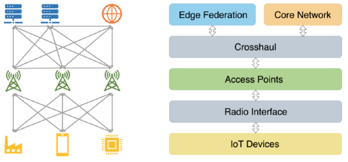
Figure 1: Mercury fog computing model.

In general terms, Mercury’s fog model comprises six submodules or layers. Each layer models different network elements that compose the fog computing scenario.

The IoT Devices layer contains all the User Equipment (UE) devices of the scenario. UE devices are mobile, and hence their position may change over time. UE may run one or more applications, and due to hardware limitations - e.g., computational power -, they require the transfer of resource-intensive tasks to an external computing platform. Mercury is primarily thought for data stream-oriented IoT applications, as these could benefit the most from fog computing. Data stream-oriented IoT applications are defined as applications that produce large amounts of data that have to be processed computation-intensively in real-time - e.g., video streaming [19].

Computation offloading is hosted on the Edge Federation layer. It is comprised of several EDCs located within the RAN under study. These EDCs contain multiple processing units, which are the hardware that provide the processing capacity to their corresponding EDC. For modeling how computation offloading is performed in Mercury, we based our model on the FaaS concept, also known as serverless [20]. In FaaS environments, there are not resources reserved for any application; the infrastructure will start a process only when a client makes a service request. Due to location-awareness particularities of fog computing, implementing FaaS-based applications may optimize resource pooling and elasticity, security, provisioning, and management at scale [11].

In Mercury, a UE may implement one or more applications. Each application generates a data stream. We refer to a service as the computation offloading for processing the data stream of an individual UE application. When a UE starts a service, it sends a create session request to one of the EDCs of the edge federation. A session consists of reserving computing resources temporarily for the exclusive processing of data flows from a given service. In this way, enough computing resources are granted until the UE terminates the session. Once a session is closed, computing resources are released and available for any other potential new service.

UE connect to the RAN via Access Points (APs) scattered around the scenario. These APs are gathered in the Access Points layer. APs also manage the Radio Interface layer’s resources. This layer interconnects UE with APs. The Core Network layer gathers the functions that are to be performed within the ISP’s core network. These functions are enforcing access control policies in the RAN and configuring the Crosshaul layer interconnections. The Crosshaul layer interconnects EDCs, APs and the core network functions.

3.2 Allocation Manager

Mercury’s fog model is flexible, configurable, and allows modeling complex and detailed scenarios with great detail. However, this tool may be used for straightforward, standard use cases. To make it easier for the user to configure the fog layers, Mercury offers an Allocation Manager, a set of automatic tools to optimize the configuration of the model to be explored. The allocation manager provides scenario optimizations to find the most suitable locations for APs and EDCs depending on UE modules’ location histogram, as shown in Figure 2.

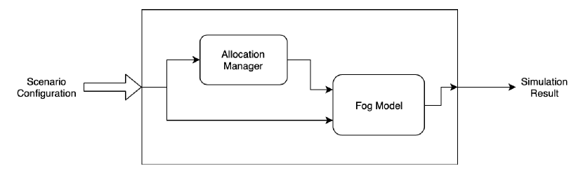
Figure 2: Mercury framework.

The allocation manager splits the UE location history into spatial cells with length and width of a configurable spatial resolution. For each of these cells, the allocation manager generates temporal snapshots using a given time window. For each of these snapshots, the number of unique UE nodes is computed. Finally, the allocation manager generates a density map composed of the snapshot with the highest number of UE devices for each cell. Then, a modified K-Means algorithm [21] is computed against the resulting density map. The algorithm is tuned to find solutions with a similar amount of UE density per cluster, thus evenly dividing network traffic among APs. Finally, the position of the EDCs is obtained using the standard K-Means algorithm on the APs’ locations.

4 Detailed Model Implementation

Mercury’s model for simulating fog computing scenarios is built on top of DEVS. DEVS is a general formalism for discrete event system modeling based on set theory [22]. The DEVS formalism provides the framework for information modeling, which gives several advantages to analyze and design complex systems: completeness, verifiability, extensibility, and maintainability. Once a system is described in terms of the DEVS theory, it can be easily implemented using an existing computational library. There are two types of DEVS models: atomic and coupled. Atomic DEVS models process input events based on their model’s current state and condition. They also generate output events and transition to the next state. Coupled models are the aggregated composition of two or more atomic and coupled models connected by explicit couplings.

DEVS was selected since its formalism allows the specification of a modular and hierarchical design, supports scalability and reusability, provides simple and clear semantics for the basic model behavior, and represents an explicit separation between the model specification and its corresponding implementation. To develop Mercury, we addressed MBSE methodologies. The elements and functionalities required for modeling the scenario were identified, decomposed, and characterized before implementing them. In particular, system specification was supported with Systems Modeling Language (SysML) diagrams. SysML is a general-purpose graphical modeling language for analysis, specification, design, verification, and validation of systems. This section describes each of these implementations in detail.

To implement the previously defined model, we built Mercury on top of xDEVS [23], a DEVS-compliant package for C++, JAVA, and Python 3. In this case, Mercury has been implemented using the xDEVS/Python API. Conceptually, DEVS separates models from the underlying simulator, making it possible to simulate the same model using centralized, parallel, or distributed execution modes. In this regard, DEVS models are easily distributed since tasks can be executed in different nodes because these tasks do not share memory. As a result, the net-centric xDEVS library allows a complex DEVS model to be executed in a sequential, parallel, or distributed manner, without modifying the underlying Mercury model. The difference consists of running the simulation using the same root Coupled model, but through the Coordinator class (sequential simulation), the CoordinatorParallel class (parallel simulation using threads), or the CoordinatorDistributed class (distributed simulation using sockets).

4.1 Structure and Behavior

As stated in Section 3, Mercury’s fog model is divided into six different layers. Each layer contains submodules that define the layer’s behavior. This section explains the structure and behavior of the key submodules for each layer.

4.1.1 Edge Federation Layer

This layer contains all the EDCs that compose the edge federation. The edge federation controller monitors the status of all the EDCs and reports it to the ISP for network management purposes. Every EDC can be divided into three different main submodules: processing unit(s), resource manager, and data center interface. Figure 3 shows a SysML Internal Block Description (IBD) of an EDC.

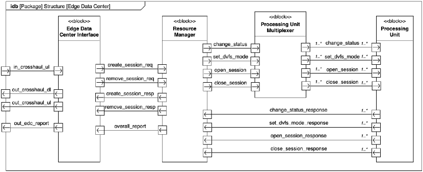
Figure 3: Edge Data Center internal block diagram.

Processing Units

These elements are hardware units - e.g., Graphics Processing Units (GPUs)- that provide computing resources to an EDC. A processing unit has a certain amount of computing resources depending on its architecture - e.g., memory and working clock frequency. Also, it has a Dynamic Voltage and Frequency Scaling (DVFS) table, which is a set of possible hardware configurations of the processing unit. Depending on the selected hardware configuration, the processing unit’s available resources and power consumption may vary: setting energy-saving configurations diminishes the demanded power for a processing unit to operate; however, its computing resources cannot be exploited entirely, as these configurations - e.g., lower clock frequency or voltage - reduce the number of instructions per second that can be performed. In general, depending on the percentage of computing resources under use, a processing unit can change its DVFS configuration for reducing power consumption while meeting computing demand. Figure 4 shows the State Machine (STM) that describes the behavior of a processing unit.

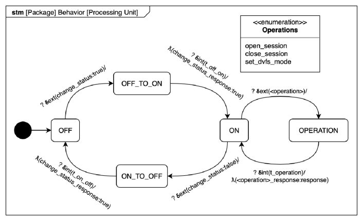
Figure 4: Processing unit state machine.

The EDC power consumption is modeled as the summation of the power consumed by all the processing units in the EDC. If a processing unit is powered off, its power consumption is zero (see Equation 1). However, it cannot host any session: a processing unit is active only when switched on. Equation 2 provides the instantaneous power of a processing unit, where u(t) is its utilization - i.e., used computing resources at time t - and DVFS(t) is the DVFS configuration used at the same instant.

$$P_{p.u.}(t)= 0$$ if p.u. is powered off (1)

$$P_{p.u.}(t)=$$ f(u(t), DVFS(t)) otherwise (2)

Resource Manager

It is in charge of controlling all the processing units. When a session creation request is received, the resource manager decides on which processing unit the session is going to be hosted. It is possible to define different session dispatching algorithms, prioritizing power consumption or QoS, for instance. Mercury incorporates by default two different dispatching algorithms: MinimumWorkloadStrategy, which forwards new sessions to the processing unit with lower utilization, and MaximumWorkloadStrategy, which dispatches new sessions to the processing unit with highest utilization - provided that it has enough available computing resources for hosting the new session. However, new dispatching algorithms can easily be defined for tailored purposes. The resource manager is also responsible for managing the DVFS mode and switching the processing units on and off when required.

Data Center Interface

This module controls the interaction with other submodules - i.e., APs and UEs-, adding networking capabilities to the EDC. Messages from the EDC are encapsulated as physical packets with transmitted power, used bandwidth, spectral efficiency, and frequency carrier. The data center interface also applies a transmission delay to messages depending on their data size. On the other hand, physical packets received from the crosshaul layer are decapsulated, their type is detected, and then they are forwarded through the correspondent port.

4.1.2 Core Network Layer

This layer gathers the tasks that are to be performed within the ISP’s core network. For accurately modeling a fog computing scenario, two functions were implemented: the Access and Mobility Management Function (AMF), which checks access permissions for any UE that requests to connect to the RAN, and the Software-Defined Network (SDN) controller, which configures the links between APs and EDCs based on proximity and EDCs’ availability.

4.1.3 Access Points Layer

This layer comprises all the APs. Figure 5 shows the IBD of an AP.

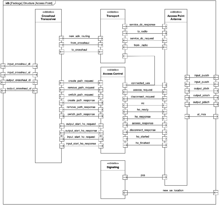
Figure 5: Access Point internal block description.

The Signaling module is responsible for emitting Primary Synchronization Signal (PSS) messages for broadcasting the AP’s information. The Access Control module administers UE’s connections and triggers handover processes when required. Moreover, the Transport module handles the routing paths of sessions between UEs and EDCs. The Crosshaul Transceiver submodule controls the interactions with the EDCs and the core network functions. Its behavior is the same as the EDC’s data center interface.

Finally, the Access Point Antenna module adapts messages that interact with the radio interface layer. Due to the particularities of radio interfaces, the behavior of this module differs significantly from the crosshaul transceiver: first, the radio spectrum is shared among every UE connected to the AP, and the bandwidth for each radio link may vary: the more devices connected to an AP, the lower available bandwidth for each of them. Mercury incorporates a predefined bandwidth share algorithm that distributes the available bandwidth evenly between the connected UE nodes. However, it is possible to define a custom bandwidth share algorithm. Figure 6 shows a schematic of how the predefined bandwidth share algorithm works.

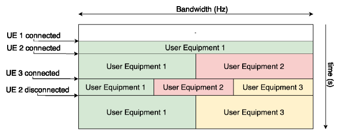
Figure 6: Access Point bandwidth assignment schematic.

Moreover, as UEs may change their position, the radio link quality changes during the simulation. This may lead to a variation in the Modulation and Codification Scheme (MCS) used for that channel, and therefore either improve or worsen the radio link’s spectral efficiency. The AP antenna monitors the radio uplink quality of the UEs connected to the AP and determines which MCS must be used depending on the perceived Signal-to-Noise Ratio (SNR). The available MCSs can be defined by the user. However, by default, the 5G New Radio (NR) MCS table is used [24].

4.1.4 IoT Devices Layer

This layer contains the UEs that are defined in the scenario. Each UE is divided into five submodules, as shown in Figure 7.

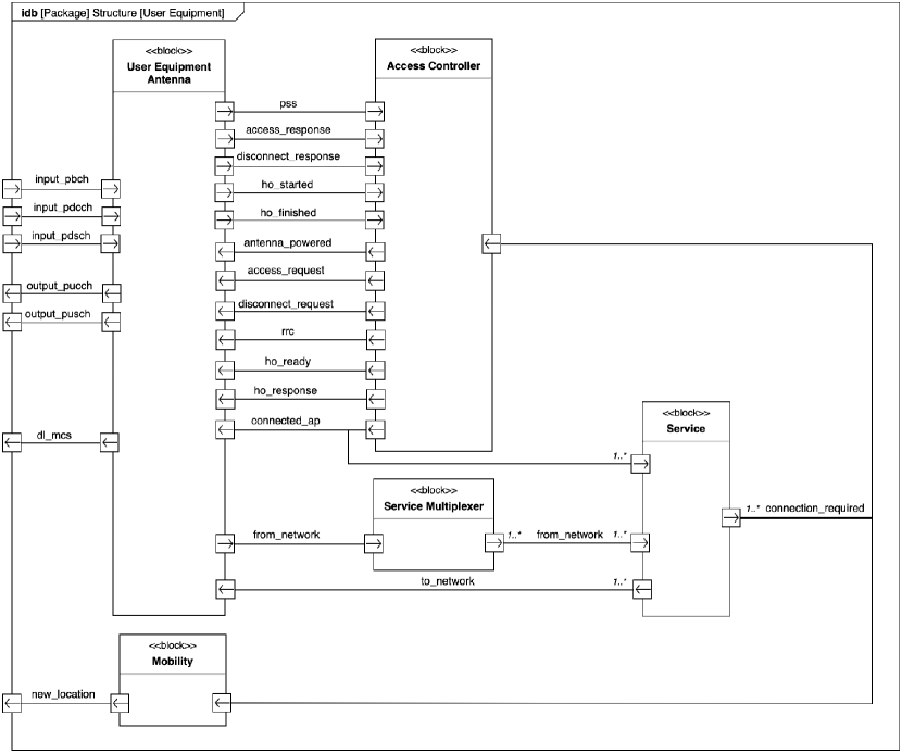
Figure 7: User Equipment internal block description.

The mobility module is in charge of managing the UE’s location. The UE antenna is similar to the AP’s, but it monitors the downlink quality instead of the uplink, and it does not configure the available bandwidth but adapts to decisions made by the APs. The access controller is responsible for connecting to the RAN. It discovers available APs, starts the access sequence, and handles handovers. Figure 8(a) shows the STM that models the behavior of the access controller. Finally, each UE has one or more service submodules. Each service submodule models the behavior of an IoT application service. Figure 8(b) shows the STM that models the behavior of a service.

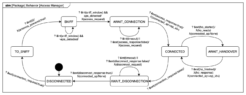
(a) UE access controller state machine.

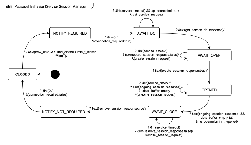
(b) UE service state machine.

Figure 8: User Equipment-related state machines.

4.1.5 Crosshaul Layer

This layer models a 5G-based transport network that combines backhaul and fronthaul, enabling a flexible software-defined reconfiguration of all the networking elements [25]. The crosshaul layer allows event transmission between Access Points, Core Network, and Edge Federation layers. The objective of this layer is twofold: on the one hand, it applies a power attenuation function to all the messages that go through it. Besides, it is also in charge of applying the corresponding propagation delay to communications. The crosshaul layer is composed of two channels that conform a Frequency Division Duplexing (FDD) full-duplex channel for data transmission between modules: one for uplink and other for downlink communications.

4.1.6 Radio Interface Layer

This layer interconnects the Access Points and IoT devices layers. Its behavior is similar to the crosshaul layer. We considered the NR physical interface [26] as a base for modeling this layer. Five physical radio channels compose the radio interface: one of them is the Physical Broadcast Channel (PBCH), which is used by APs for broadcasting PSS messages. The Physical Uplink Control Channel (PUCCH) and Physical Downlink Control Channel (PDCCH) are used for transmitting control messages - e.g., access requests and responses or handover-related messages. Finally, the Physical Uplink Shared Channel (PUSCH) and Physical Downlink Shared Channel (PDSCH) constitute a FDD full-duplex channel for data transmission between APs and UE.

4.2 Inter-module Communications

In this subsection, the interactions between the main submodules of Mercury’s fog model are explained.

4.2.1 Radio Access Network Connectivity

UE need to be connected to the RAN to successfully establish a service session with an EDC of the edge federation. UE connect to the RAN via the APs that are scattered around the scenario. First, every UE listens to PSS messages from all the APs. These messages contain information about the emitter AP and enable the UE to detect which AP offers the best radio signal quality. Eventually, UE send an access request message to their most suitable AP. APs forward these requests to the ISP’s core network, where the AMF checks the access control policies before granting the access. Once the UE receives an affirmative response to its access request, it is connected to the RAN via the selected AP. Figure 9(a) shows a sequence diagram of the connection process. For disconnecting from the RAN, the communication sequence is similar.

As UE’s location may change over time, the most suitable AP can also change. Hence, UE modules send periodic Radio Resource Control (RRC) messages to their correspondent AP. If the AP finds another more suitable AP, it triggers a handover process for transferring the UE’s session to the new AP. Figure 9(b) presents the sequence diagram for the APs handover process.

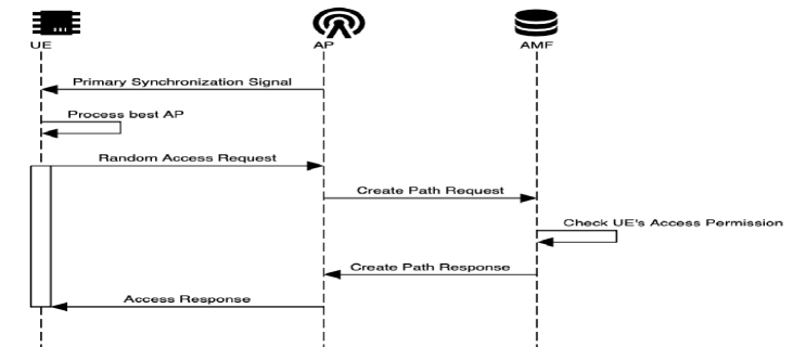
(a) UE access request sequence diagram.

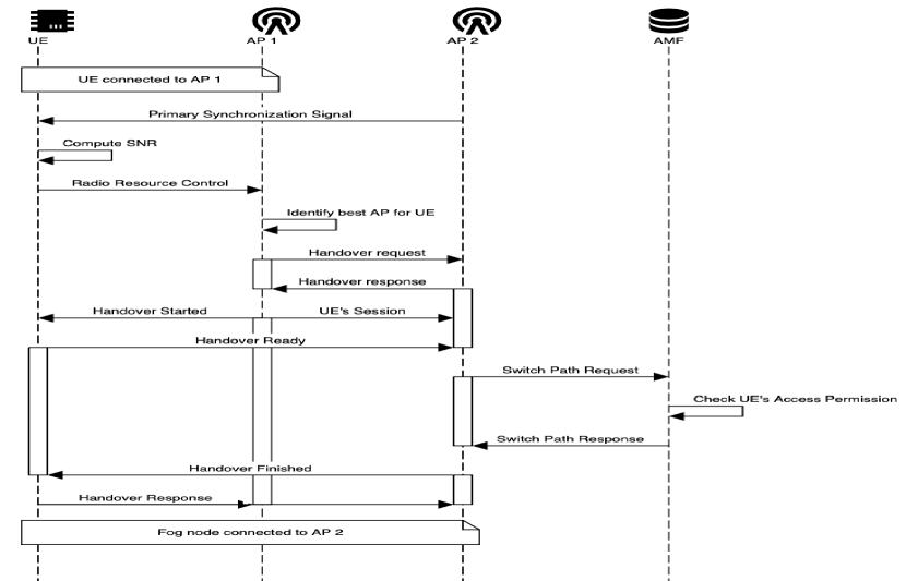
(b) UE handover sequence diagram.

Figure 9: UE connection sequence diagrams.

4.2.2 Service-Related Communications

Once the connection to the RAN has been established, the UE proceeds to ask to its AP for the most suitable EDC for each of the implemented applications. APs have an internal list of the most suitable EDC depending on the application requested. This table is generated by the SDN controller, which is in charge of providing network slicing capabilities to the RAN. The table changes dynamically depending on the federated EDCs’ available resources.

UE then send one session creation request per service to the correspondent EDC. The EDC that receives the request checks if there are enough resources for the new service session request, and allocates the resources if available. The EDC sends an affirmative response to the UE so it can transfer the service-related data stream, which is processed in real-time. The UE voluntarily closes the session after a timeout to avoid resource starvation, repeating the entire service request process. Note that the highest delays experienced by the UE occur when creating and removing a session. Once a session is opened, requests are quickly processed. Figure 10 shows a sequence diagram of a single service.

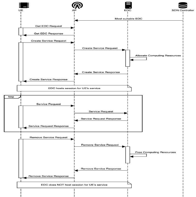
Figure 10: Service operations sequence diagram.

5 Use Case

In this section, we propose a use case scenario to show how Mercury can assist with the dimensioning and operation tasks during the deployment of new edge computing infrastructures. The output generated by the M&S framework is analyzed to give a sense of how it can be interpreted to help on the decision-making process. Finally, we show how the proposed scenario could be explored using other M&S frameworks to stress the novelty and major advantages of Mercury.

5.1 Scenario Description

To analyze the performance of the model presented in this research, we propose a driving assistance scenario. ADAS scenarios provide a dynamic real-time data stream analytics environment that handles large volumes of data. Each vehicle is running an onboard predictive model that detects potentially dangerous situations according to real-time images from the driver’s face. The purpose of this use case is to keep training the predictive model for each vehicle to capture the particularities of every driver, improving the accuracy of the predictive model in a personalized way. Training machine learning models is a computationally expensive process, and using computation offloading could improve the overall performance while reducing the service deployment cost: pools of specialized hardware resources are shared between all the users of the application, thus making unnecessary to include extra expensive hardware in the vehicle. The usage of an edge federation for computation offloading benefits from reducing latency and core network traffic, as data is sent to EDCs that are closer to the data sources. Figure 11 shows a schematic of the proposed use case. UEs (vehicles) periodically send images in real-time to be processed by EDCs, which train a custom predictive model for each vehicle, thus reducing the risk of an accident occurring. To do so, EDCs inject in real-time the new images sent by vehicles to the training process. Once the trained predictive models are significantly improved compared to the onboard versions, the embarked models can be upgraded during run-time. Note that each vehicle is in motion and that the model will manage the necessary AP and EDC allocation changes to ensure QoS in the image data flow.

Figure 11: Use case schematic.

To present a realistic scenario, we feed our model with real mobility traces provided by EPFL (Piorkowski et al. [27]). The dataset contains mobility traces of taxis in San Francisco, USA. The trace set provides 30 days information about GPS coordinates of 500 taxis. Due to the high volume of data, we constrain the dataset to the area of the bay during the busiest 10 minutes of the peak hour of the day with the highest traffic flow (18:30:00 to 18:40:00 on 6 June 2008, PDT, UTC -7:00, daylight saving time). Our resulting dataset presents 100 vehicles that are in our target area during all the simulation time. As the original data are presented at a rate of approximately one trace per minute, we have performed a linear interpolation to obtain a final rate of one trace approximately every 10 seconds to increase the granularity of the scenario. Finally, we transform GPS data to cartesian coordinates with an error lower than 10 centimeters per kilometer. Figure 12 shows the taxis’ interpolated location history during the 10 minutes to be simulated in cartesian coordinates.

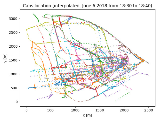
Figure 12: Taxis location during simulation time.

Regarding the ADAS service, each vehicle sends a large volume of data corresponding to a real workload from the Elektra Autonomous Vehicle database [28]. We use the CVC11 Driver Face dataset, which compiles Standard Definition (SD) images from onboard cameras using a resolution of 640x480 pixels. The images feature male and female driver’s faces while driving in real scenarios. These images are processed in the EDCs computing infrastructure to train a classification model for accident prevention. The required binary rate is modeled as 1 Mbps.

The ADAS service configuration parameters are as follows: after idling during one second, each UE sends a “create service” request. If the UE does not get a response after 0.35 seconds, it resends the request. After creating the service, each UE sends a “service request” message every second. These messages have 1 Mbit size, thus resulting in a binary rate of 1 Mbps per vehicle. Once 20 messages (around 20 seconds) are transmitted and replied, UE nodes demand a session removal and idle for another second. Each UE repeats the entire process until the end of the simulation.

The EDCs’ computing resources consist of a set of GPUs of the Sapphire Pulse Radeon RX 580 series. GPU-based clusters are one of the best options to provide the workload requirements demanded by ADAS applications, as they run Deep Neural Networks (DNNs) and Convolutional Neural Networks (CNNs), frequently used for training classification models, with a significantly higher performance than Central Processing Units (CPUs) [29]. The workload consists of training the classification model, including the received images, which is based on a CIFAR-10 model. The images used for training the model are from the ADAS dataset from Elektra Autonomous Vehicle. Each GPU can host the sessions of up to five vehicles simultaneously - i.e., sessions require 20% of its computing resources.

We use a GPU power model based on an Artificial Neural Network (ANN) that depends on the current ADAS workload. The performance of this power model presents a Normalized Root Mean Square Deviation (NRMSD) of 2.45% and an $R^{2}$ of 99.01%. The time required for powering on/off the GPUs is set to 1 second. For starting or removing a session, a GPU needs 0.2 seconds.

APs antennas transmitting power was set to 50 dBm, their gain to 0 dB and their equivalent noise temperature to 300 K. UE’s gain and equivalent noise temperature coincided with the APs’, but their transmitting power was limited to 30 dBm. Regarding the radio interface frequency band, the default value provided by the allocation manager is used, which is the n77 band - carrier frequency of 33,000 MHz and bandwidth of 100 MHz per channel.

5.2 Scenario Optimization

Due to the scenario’s complexity, we used Mercury’s allocation manager automatic tools. The number of APs, as well as their location, were automatically set by the allocation manager. With a time window of 1 second and a spatial resolution of 40 meters, the allocation manager built the density map shown in Figure 13, placing 10 APs in the locations spotted with yellow stars.

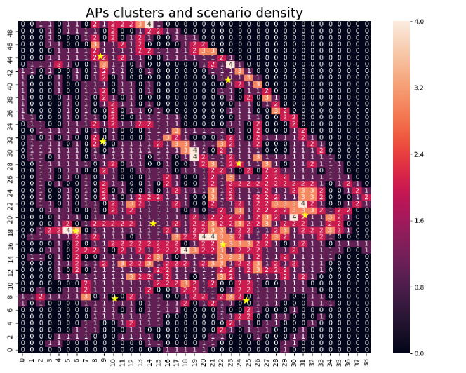
Figure 13: San Francisco scenario density.

Regarding the EDCs, the allocation manager determined that each EDC should have 20 GPUs (5 sessions/GPU $\times$ 20 GPUs = 100 sessions). As we set the replication factor to 3 - value for ensuring a high availability infrastructure -, the scenario ended up with three EDCs. The final scenario is shown in Figure 14, where thick dots present the EDCs, and the APs are displayed as stars. The colors of the dots and the stars define the EDCs’ preferred activity region.

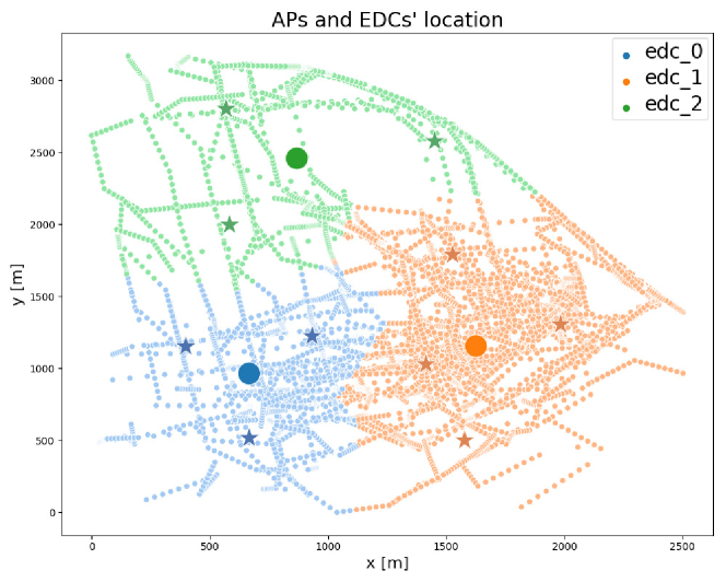
Figure 14: San Francisco final scenario.

5.3 Experiments Definition

To show how Mercury can assist on the analysis of the dynamic operation strategies for edge federations, we present two different experiments that differ in the EDCs’ resource manager configuration. The target of the first experiment is to reduce the delay perceived by UE. For doing so, all the GPUs were powered on during the whole simulation. The selected dispatching algorithm was the MinimumWorkloadStrategy, as it was the one that reported the best QoS results in previous use cases [13]. On the other hand, the second experiment keeps switched off idle GPUs and uses the MaximumWorkloadStrategy for reducing overall power consumption. Both dispatching strategies are presented in Section 4.1.1. Table 2 resumes the selected configurations for both experiments. Simulations were executed using PyCharm Professional 2019.1.1 [30] on a MacBook Pro (Retina, 15-inch, Mid 2015) with a 2.5 GHz Intel Core i7 processor and a 16 GB 1600 MHz DDR3 memory. Each simulation took approximately 10 hours and 30 minutes.

Table 2: Configuration of San Francisco experiments.

	Unused Hardware Strategy	Dispatching Strategy
Experiment I	Powered on	MinimumWorkloadStrategy
Experiment II	Powered off	MaximumWorkloadStrategy

5.4 Simulation Results

After simulating both experiments, it is possible to analyze both outcomes quantitively in terms of available bandwidth, power consumption and perceived delay. The only difference between the two experiments resided on the EDCs’ dispatching algorithm. However, as the location of both APs and UE devices were the same, each UE was connected to the same APs during both simulations, and the bandwidth share, as well as the applied MCS, coincided. Due to this, the uplink and downlink bandwidth and bit rate perceived by UE modules in both experiments is the same, as shown in Figure 15.

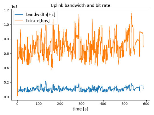
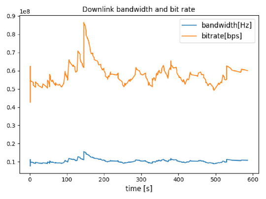
Figure 15: Radio interface bandwidth and bit rate in San Francisco scenario.

In both cases, the bandwidth ranges from 9 to 12 MHz, with a peak of 16 MHz. Provided that the scenario has 10 APs and there are 100 taxis, ideally only 10 UE devices would be connected to a single APs, thus having 10 MHz - the total available radio bandwidth is 100 MHz per AP. Therefore, we can conclude that the bandwidth share is achieved with Mercury’s allocation manager. Downlink bandwidth and bit rate, though in different scales, match during all the simulation. The reason for this is that the downlink spectral efficiency is 5.5547 bps/Hz throughout the simulation. When comparing it to the MCS table of the NR interface [24], it can be seen that it coincides with the MCS with the highest spectral efficiency. As the transmitting power of the APs is high, and the maximum downlink modulation is 64-Quadrature Amplitude Modulation (QAM), the downlink quality is good enough to provide always the best efficiency. On the other hand, the transmitting power of the UE nodes is not enough for granting the best spectral efficiency. Moreover, modulations in the uplink may reach 256-QAM, a more complex modulation that requires better SNR to be used. Depending on their distance to the AP they are connected to, the used MCS varies. Figure 16 shows the uplink spectral efficiency of the proposed scenario.

Figure 16: Radio interface uplink spectral efficiency and bit rate in San Francisco scenario.

Table 3 gathers different simulation metrics for comparing both experiments. Experiment II reported 28% less power consumption than the first experiment - see Figure 17. This is due to the first experiment’s unused hardware strategy and dispatching algorithm, which keep all the processing units switched on during the whole simulation. On the other hand, in experiment II, unused processing units are switched off, and sessions are dispatched to already switched on processing units if enough resources are available.

Table 3: Real scenario simulation results.

	Experiment I	Experiment II
Mean Perceived Delay (ms)	35.35	39.31
Peak Perceived Delay (ms)	496.18	2,519.80
Mean Power Consumption (kW)	6.04	2.33
Peak Power Consumption (kW)	6.10	2.41

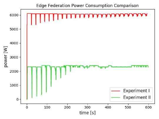
Figure 17: Comparison of EDCs power consumption in San Francisco scenario.

Focusing on the perceived QoS, the mean delay perceived in experiment I is 3.96 ms less than in experiment II, which a priori might not seem a significant difference. However, the second experiment registered a peak delay of 2.52 seconds, in contrast with the peak delay of 0.50 seconds for the first experiment - i.e., the first configuration provides a better and more predictable QoS. Figure 18 compares the perceived delay in both scenarios.

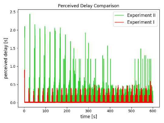
Figure 18: Comparison of delay perceived by UE devices in San Francisco scenario.

As shown in this subsection, Mercury includes built-in visualization tools for analyzing during run-time the scenario outline, bandwidth share, binary rate, perceived delay, and federation power consumption simulation outcome. Furthermore, Mercury incorporates transducers for storing any simulation event in Comma-Separated Values (CSV) files in case a more in-depth analysis is required. With this output, it is possible to make design decisions depending on the application under study and its particular technical requirements. Note that the objective of this paper is to exemplify the workflow of Mercury, as well as its novelties compared to other available M&S frameworks.

5.5 Comparing Mercury With Other Simulators

To compare Mercury with other alternative fog computing simulation tools, we defined similar scenarios and analyzed their output. Specifically, we studied iFogSim [18] and EdgeCloudSim [17], since these simulators allow defining generic use cases, as shown in Table 1. All the scenarios were comprised of 100 UEs and three EDCs. Other configuration parameters were dependent on the simulator under study. Since it is not possible to specify exactly the same model of the use case in the different M&S frameworks, an in-depth numerical comparison between the results obtained by Mercury and by the other M&S frameworks is out of the scope of this research.

5.5.1 iFogSim

iFogSim does not include any spatial conception in its model: all the elements are interconnected in a tree-based fashion. Communication links are modeled as dedicated lines between a parent node and each of its children. These links have independent uplink and downlink bandwidth, as well as a fixed communication delay. Node mobility is not implemented, and therefore the tree does not change during the simulation. In contrast, in Mercury, the connections that reduce the perceived latency are selected dynamically depending on the location of the elements and the instantaneous status of the edge computing federation. Mercury’s behavior coincides with the vision of 5G, in which networks have cognitive functions that enable them to adapt themselves to the current state of the infrastructure.

In iFogSim, the user must establish the data flow of the application under study. This feature enables us to define more complex behaviors based on request-response communication patterns, which is a useful feature for exploring how fog computing particularities would affect to a given application. Again, this differs from Mercury, which is focused on data stream-oriented applications, where the state machine that defines their behavior is the same for all of them. In Mercury, only timing and data size-related parameters can be configured.

The power consumption model of EDCs in iFogSim consists of idle and active power consumption. On the other hand, Mercury enables us to define more complex power models in which processing units within the EDCs can be powered on/off and the instantaneous power consumption depends on the utilization and DVFS configuration. Two of the EDCs in the scenario had three children APs, while the other had four instead. Each AP had 10 children UEs. The wall-clock execution time of iFogSim was 272 milliseconds, outperforming Mercury’s. It is worth to mention that, with iFogSim, we can neither get nor set information about simulation time.

iFogSim’s outcome provided information regarding the average delay and power consumption, but no real-time progression is shown. As a consequence, we cannot extract the temporal behavior of our scenario with iFogSim. Gathering data with respect to the temporal behavior of all the components in the simulation process is necessary to define some management policies regarding hardware configuration as a function of isolated hot spots like power consumption peaks, network congestion, etc.

5.5.2 EdgeCloudSim

In EdgeCloudSim, APs and EDCs are tied together, and each EDC defined by the user implicitly involves an AP with its independent WLAN. EDCs are interconnected via a MAN. In contrast with Mercury, cloud computing is also part of EdgeCloudSim’s model. All the EDCs are connected to the cloud through a WAN. If an EDC runs out of computing resources, computing offloading can be triggered to other EDC or to the cloud - at expenses of drastically incrementing the perceived delay.

EdgeCloudSim enables the user to define a minimum and a maximum number of UEs, and several scenarios are simulated exploring different UE densities in this range. Mobility is also managed internally by the simulator, and therefore it is not possible to define trajectories. UEs are always connected to their closest AP, and mobility may lead to a handover. However, the handover is not modeled in detail: there is no AP discovery process nor radio link quality monitoring. In addition, UE location does not affect the available bandwidth nor its spectral efficiency. In Mercury, the propagation delay is proportional to the distance between UE and their correspondent AP. Besides, in our research, the radio spectrum is shared among UE connected to the same AP- i.e., transmission delay varies in simulation time. Furthermore, in Mercury, the spectral efficiency of the communications may vary depending on the SNR.

We defined a scenario with three pairs of EDCs and APs. Mobility was enabled for all the UE in the scenario. The simulation time was set to 10 minutes, and it took one second of execution time, outperforming Mercury’s. However, EdgeCloudSim does not support power consumption models, and this aspect was not explored. Moreover, as in iFogSim, no temporal data is gathered: EdgeCloudSim provides average measurements about the tasks executed on EDCs and cloud, and about which tasks succeeded and which failed due to either lack of computing resources or mobility issues.

5.5.3 Comparison Remarks

In conclusion, one of iFogSim’s most appealing features is the exploration of the effect of fog computing on a given application. It enables the user to define complex request response communication sequences and explores how computing offloading can be performed across the network. iFogSim gives a sense of the mean latency experienced by the application. This framework also provides a coarse-grained intuition of the power consumption of the infrastructure. On the other hand, EdgeCloudSim’s strongest point is that it allows exploring the average QoS experienced by a different number of users depending on the available computing resources. It is useful for a first approach of the edge computing infrastructure dimensioning depending on the expected demand. However, information about power consumption is not provided.

Mercury is a framework for fine-grained edge infrastructure dimensioning and operation tasks. It focuses on data stream-oriented applications. Mercury incorporates optimization tools for assisting in the most suitable location of edge computing infrastructure. This M&S&O framework provides a wide range of real-time data - e.g., the usage of the network and the computing resources, perceived delay, and bandwidth share. It is possible to study the implications of using different dispatching and hardware management techniques within the EDCs that comprise the edge computing federation. Therefore, Mercury helps to diminish the impact of hotspots, leveraging the usage of computing resources in a location-aware manner. It could impact positively on the operational expenses and the QoS of future fog computing deployments.

6 Conclusions and Future Work

In this research, we present Mercury, an M&S&O framework to analyze the dimensioning and run-time operation of edge federations in fog computing scenarios. Our framework is designed using MBSE methodologies together with the DEVS mathematical formalism, providing an explicit separation between the model specification and its corresponding implementation. When defining a complex system, this formalism helps to isolate the detailed specification of its elements in terms of structure, behavior, and their relationships, providing an atomic verification for all of them.

On the one hand, Mercury provides a fine-grained hierarchical model of fog computing environments. The fog computing paradigm provides a solution for distributing the computing infrastructure geographically, closer to data sources. Mercury also includes a set of automatic tools for assisting with the physical location of these infrastructures in the Radio Access Network.

Our model supports location awareness, inherent in fog computing, through a FaaS/serverless model that dynamically allocates application service requests. This enables the definition of fine-grained energy efficient strategies due to on-demand resource provisioning. In contrast with other M&S tools, Mercury is focused on data stream analytics-based services, as fog computing appears as a technology enabler for this type of applications.

IoT devices’ mobility is natively supported by Mercury, which models a federated management of computation offloading that adapts resource allocation to the geographical application demand profile with the aim of optimizing the perceived QoS. Inter-module communication models are based on the 5G standard to reflect the impact of networking technologies on the application performance, gathering the effects of bandwidth share, packet loss, perceived delay, and connectivity protocols.

On the other hand, Mercury is implemented on top of the Python 3 distribution of xDEVS, making extensive use of Abstract Base Classes for ensuring high flexibility. This M&S&O framework provides a wide range of simulation real-time data - e.g., the usage of the network and the computing resources, perceived delay, and bandwidth share. These detailed simulation outputs allows the analysis of dynamic optimization strategies in fog computing environments.

Finally, we demonstrate the novelty and major advantages of Mercury, proposing a realistic use case scenario (incorporating real data traces and validated energy consumption models), to show how our M&S&O framework can assist with the dimensioning and operation tasks during the deployment of the edge computing infrastructure. We offer as well a detailed comparison with other state-of-the-art fog computing simulators.

Mercury will assist with the dimensioning and operation of edge federations prior to actual system deployments, detecting potential bottlenecks while significantly reducing development costs.

6.1 Future Work

We are currently working on a new version of Mercury that includes a new module, the Decision Support System, to explore different configurations for the scenario elements, for instance, the number of EDCs’ processing units and the workload dispatching algorithms. We are also including a cloud layer that would be connected to the core network, in order to extend computation offloading. On the other hand, we are designing a new layer to model Machine-to-Machine (M2M) communications between neighboring UE devices aimed to enhance computation offloading and data sharing at UE level. Finally, a new smart grid layer will be developed to simulate an electrical grid with different renewable energy sources as well as the energy distribution and storage systems. Adding these new contributions to Mercury will open the possibility of studying a wide variety of new optimization issues.

References