Multiple Reference Signals Collaborative Sensing for Integrated Sensing and Communication System Towards 5G-A and 6G

Abstract

Integrated sensing and communication (ISAC) is considered as the potential key technology of the future mobile communication systems. The signal design is fundamental for the ISAC system. The reference signals in mobile communication systems have good detection performance, which is worth further research. Existing studies applied the single reference signal to radar sensing. In this paper, a multiple reference signals collaborative sensing scheme is designed. Specifically, we jointly apply channel state information reference signal (CSI-RS), positioning reference signal (PRS) and demodulation reference signal (DMRS) in radar sensing, which improve the performance of radar sensing via obtaining continuous time-frequency resource mapping. Crámer-Rao lower bound (CRLB) of the joint reference signal for distance and velocity estimation is derived. The impacts of carrier frequency and subcarrier spacing on the performance of distance and velocity estimation are revealed. The results of simulation experiments show that compared with the single reference signal sensing scheme, the multiple reference signals collaborative sensing scheme effectively improves the sensing accuracy. Moreover, because of the discontinuous OFDM symbols, the accuracy of velocity estimation could be further improved via compressed sensing (CS). This paper has verified that multiple reference signals, instead of single reference signal, have much more superior performance on radar sensing, which is a practical and efficient approach in designing ISAC signal.

I Introduction

TABLE I: Comparison of DMRS, PRS, CSI-RS and SS [20]

	DMRS	PRS	CSI-RS	SS
Sequence Generation	Gold sequence	Gold sequence	Gold sequence	M-sequence and Gold sequence
Time-frequency Domain Resources	Maximum of 4 symbols in a time slot	A time slot with 2/4/6/12 symbols; 24–272 PRBs	A time slot with 1/2/4 symbols; up to 52 physical resource blocks (PRBs)	2 OFDM symbols in a synchronization signal block (SSB); 127 subcarriers
Time-frequency Domain Configuration	Distribute as evenly as possible; 50% or 33.3% of resource element (RE) density	2/4/6/12 comb structure	When occupying 2 symbols, they must be adjacent; when occupying 4 symbols, they are divided into two parts, and the two symbols in each part are adjacent	The 1st and 3rd symbol at SSB; consecutive subcarriers
Signal Location	Uplink and downlink channel	Downlink channel	Downlink channel	SSB

The future fifth generation-advanced (5G-A) and the sixth generation (6G) mobile communication systems will provide new services such as smart factory and intelligent transportation system (ITS), which require both sensing and communication [1]. In ITS, the vehicle detects the surrounding environment and share the information such as velocity, acceleration, braking, and driving direction with base stations (BSs) to ensure safety of vehicles and pedestrians. Integrated sensing and communication (ISAC), which realizes sensing based on the mobile communication system, is promising to support these new services. One of the primary technologies of ISAC is the ISAC signal design to realize the deep fusion of sensing and communication.

Communication requires random signals to maximize the data transfer rate, while Sensing requires signals with structured and strong autocorrelation characteristics to eliminate distance and velocity ambiguity [11]. This contradiction brings challenges for ISAC signal design. There are mainly two types of ISAC signal design schemes as follows. (1) Sensing centric ISAC signal: In the sensing centric ISAC signal design, the communication data is modulated in sensing signals, for example, linear frequency modulated (LFM) signal [2][3]. The communication rate of sensing centric ISAC signal is limited. (2) Communication centric ISAC signal: The communication centric ISAC signal design is the main stream of ISAC systems towards 5G-A and 6G, which mainly adopts the orthogonal frequency division multiplexing (OFDM) based ISAC signal design [7][8]. However, the randomness of the data in OFDM signal conflicts with the required high autocorrelation for sensing, which brings challenge to high-quality sensing.

Reference signal in 5G New Radio (NR) has good detection performance and strong anti-interference ability [12], which attracts extensive attention. In [12], a positioning reference signal (PRS)-based radar sensing scheme is proposed and the performance of distance and velocity estimation is analyzed. In [13], channel state information reference signal (CSI-RS) and demodulation reference signal (DMRS) are utilized respectively for sensing and the influences of time-frequency resource mapping on the sensing performance are investigated. A time-frequency continuous pilot structure is proposed to enhance the sensing performance of existing OFDM signal in [14]. In [15], superimposed reference signal is used to estimate channel state information and detect target simultaneously. In [16], a radar signal processing method based on continuous pilot and stepped pilot is proposed to achieve accurate detection. In [17], DMRS is applied in bi-static and multi-static radars. In [18], interleaved DMRS is applied in downlink and uplink sensing using one-dimensional (1D), two-dimensional (2D) and three-dimensional (3D) compressed sensing (CS) algorithms. However, the equidistant subcarrier interleaving causes ambiguity in distance estimation. To solve this problem, the concept of multiple input multiple output-orthogonal frequency division multiplexing (MIMO-OFDM) radar with non-equidistant subcarrier is proposed in [19], maintaining unambiguously distance estimation.

However, the above researches have the following limitations. First, time-frequency resources of reference signals are discontinuous, which degrades sensing performance. Moreover, the single reference signal occupies fewer resources in time-frequency domain and are distributed in a comb shape, resulting in low sensing accuracy. If a large amount of resources are allocated to a single reference signal, it will affect the distribution of other reference signals and data signals, thereby affecting the communication performance.

Facing the above limitations, this paper proposes the ISAC signal based on the reference signals in mobile communication system. The proposed ISAC signal has the following advantages. Firstly, it makes full use of multiple reference signals through flexible parameter settings to achieve high radar sensing accuracy. Secondly, the range of maximum unambiguous distance and velocity is extended. Furthermore, it expands the sensing capability of reference signals in 5G NR. Then, Crámer-Rao lower bounds (CRLBs) of the proposed ISAC signal for distance and velocity estimation are derived. The CS-based signal processing algorithm to improve the accuracy of velocity estimation is proposed. The contributions are summarized as follows.

• DMRS, PRS and CSI-RS are jointly applied to realize radar sensing, so that the resource of the designed ISAC signal is continuously distributed in the time-frequency domain to obtain high sensing accuracy and enlarge the maximum unambiguous velocity and distance.

• We derive the CRLBs of the proposed ISAC signal for velocity and distance estimation. The performance of the proposed ISAC signal is presented from the perspectives of theoretical derivation and simulation results.

• Two-dimensional-fast Fourier transform (2D-FFT) algorithm is further improved via CS to enhance the accuracy of velocity estimation. Complete channel information matrix is reconstructed with fast iterative soft thresholding algorithm (FISTA), which is similar to the distance-velocity profile generated by continuous OFDM symbols.

The structure of this paper is as follows. The reference signals are introduced in Section II. Section III proposes the ISAC signal design and processing schemes. Section IV analyzes the resolutions and CRLBs of the proposed ISAC signal for distance and velocity estimation. Section V improves the 2D-FFT algorithm via CS to overcome the limitation of 2D-FFT algorithm on velocity estimation with discontinuous signals in time domain. In Section VI, simulation results reveal the influence of multiple parameters such as carrier frequency and subcarrier spacing on sensing accuracy. Section VII concludes this paper.

II Main Reference Signal in 5G NR

In this section, we introduce DMRS, CSI-RS and PRS in 5G NR, and analyze their time-frequency resource mapping schemes to explain their practicality in radar sensing.

II-A 5G Reference Signals

Reference signals in 5G NR mainly include CSI-RS, PRS, DMRS, synchronization signal (SS), etc., and their characteristics are shown in Table I. It is revealed that DMRS is in both uplink and downlink channels, which is the most widely distributed. The comb distribution of PRS also holds abundant resources in time-frequency domain. In order to align with DMRS and PRS in downlink channel, CSI-RS is chosen. However, SS is limited by the periodic transmission of SSB, occupying limited time domain resources.

II-B Sequence Generation of Reference Signals

TS 38.211 [20] defines the generation sequence of DMRS as

$$\small r\left(m\right)=\frac{1}{\sqrt{2}}\left(1-2c\left(2m\right)\right)+j\frac{1}{\sqrt{2}}\left(1-2c\left(2m+1\right)\right),$$ (1)

where $c$($i$) is the Gold sequence of length-31, $j$ is the imaginary unit. The initial value of $c$($i$) is

$$\begin{split}\begin{aligned} \small c_{\rm{init}}=&(2^{17}(N_{\rm{symbol}}^{\rm{slot}}n_{s,f}^{\mu}+l+1)(2N_{\rm{ID}}^{n_{\rm{SCID}}}+1)\\ &+2N_{\rm{ID}}^{n_{\rm{SCID}}}+n_{\rm{SCID}})\bmod 2^{31},\end{aligned}\end{split}$$ (2)

where $N_{\rm{symbol}}^{\rm{slot}}$ is the number of symbols in a time slot, $n_{s,f}^{\mu}\in\{0,1,\ldots,N_{{\rm{slot}}}^{{\rm{frame,}}\mu}-1\}$ is the index of time slot within frame $f$ , $N_{{\rm{slot}}}^{{\rm{frame,}}\mu}$ is the number of time slots in a frame under the subcarrier spacing parameter $\mu$, $l\in\{0,1,\ldots,13\}$ is the index of OFDM symbol mapped to a time slot, $n_{\rm{SCID}}\in\{0,1\}$ is the scrambling identity (ID) of downlink DMRS, $N_{\rm{ID}}^{n_{\rm{SCID}}}\in\{0,1,\ldots,65535\}$ is the physical layer cell ID, and mod refers to the modulo operation.

The generation sequence of PRS is the same as (1). The initial value of $c$($i$) is

$$\begin{split}\small c_{\rm{init}}=(2^{22}\left\lfloor\frac{n_{\rm{ID,seq}}^{\rm{PRS}}}{1024}\right\rfloor+2^{10}(N_{\rm{symbol}}^{\rm{slot}}n_{s,f}^{\mu}+l+1)\cdot\\ (2(n_{\rm{ID,seq}}^{\rm{PRS}}\bmod 1024)+1)+(n_{\rm{ID,seq}}^{\rm{PRS}}\bmod 1024))\bmod 2^{31},\end{split}$$ (3)

where $n_{\rm{ID,seq}}^{\rm{PRS}}\in\{0,1,\ldots,4095\}$ is the scrambling ID of downlink PRS. Other parameters have the same meaning as the DMRS sequence.

The generation sequence of CSI-RS is the same as (1). The initial value of $c$($i$) is

$$\small c_{\rm{init}}=(2^{10}(N_{\rm{symbol}}^{\rm{slot}}n_{s,f}^{\mu}+l+1)\cdot(2n_{\rm{ID}}+1)+n_{\rm{ID}})\bmod 2^{31},$$ (4)

where $n_{\rm{ID}}$ is the scrambling ID of the downlink CSI-RS. Other parameters have the same meaning as the DMRS sequence.

II-C Resource Mapping Schemes

The mapping type of DMRS determines the symbol start position of DMRS in time domain. In this paper, we choose the mapping type A [20], in which the first DMRS symbol is located at symbol #2 in a time slot. After selecting mapping type in time domain, we continue to configure the resources in frequency domain for DMRS. The configuration type of DMRS determines the RE density of DMRS in frequency domain. In order to occupy more frequency domain resources, we choose type 1 [20], in which RE of DMRS is distributed in frequency domain with the density of 50 %.

5G NR system adopts the DMRS structure combining front-loaded DMRS (fro-DMRS) and additional DMRS (add-DMRS) [20]. The position where the fro-DMRS first appears should be close to the starting point of scheduling, so as to reduce delay of demodulation and decoding. In high-velocity vehicle scenarios, more DMRS symbols need to be inserted to meet the estimation accuracy of the time-varying channel, namely, add-DMRS. This paper chooses one single fro-DMRS and three add-DMRS mode, which has abundant time-frequency domain and brings high sensing accuracy. Thus, the time-frequency resource mapping diagram of DMRS in a time slot (14 consecutive OFDM symbols) and a PRB (12 consecutive subcarriers) is shown in Fig. 1.

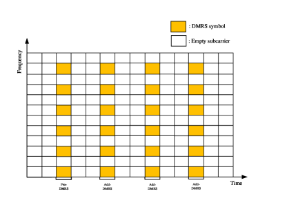
Figure 1: Single DMRS symbol plus three additional DMRS symbols

According to resource mapping scheme of PRS defined in [20], PRS supports 2/4/6/12 comb forms. Fig. 2 shows the time-frequency resource mapping scheme with comb 4 and 4 symbols.

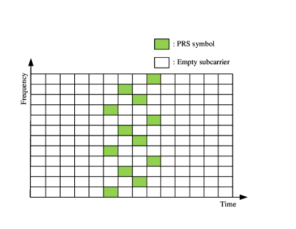
Figure 2: Resource mapping scheme corresponding to 4 symbols, comb 4

In single-input single-output (SISO) system, a single-port CSI-RS occupies a single RE in a time slot and a PRB. In order to align with DMRS and PRS in frequency domain, we chose 12 single-port CSI-RS, occupying 12 consecutive subcarriers in frequency domain and one OFDM symbol in time domain.

III ISAC Signal Model

The current signal of 5G NR is not natively designed for radar sensing. Analysis of the structure of reference signal reveals that the reference signal occupying consecutive subcarriers can effectively improve the accuracy of distance estimation, and the reference signal occupying consecutive symbols can improve the accuracy of velocity estimation, so that multiple reference signals collaborative sensing scheme is proposed to realize nearly consecutive time-frequency resource mapping, therefore improving the accuracy of distance and velocity estimation.

The reference signal occupying $M_{J}$ OFDM symbols and $N_{J}$ subcarriers is

$$\small x(t)=\sum_{m=0}^{M_{J}-1}\sum_{k=0}^{N_{J}-1}\mathbf{s}(k,m)e^{j2\pi f_{k}t}{\rm{rect}}(\frac{t-mT_{\rm s}}{T_{\rm s}}),$$ (5)

where $\mathbf{s}$ is the modulation symbol of reference signals, $k$ is the index of subcarrier, $m$ is the index of OFDM symbol, $T_{\rm s}=T+T_{\rm{cp}}$ is the total duration of OFDM symbol with $T$ representing OFDM symbol duration and $T_{\rm{cp}}$ representing cyclic prefix (CP) duration, $f_{k}$ is the $k$-th subcarrier carrying the reference signal, and ${\rm{rect}}(t/{T_{\rm s}})$ is the rectangle window function.

The received echo signal includes the two-way round-trip delay and Doppler frequency shift, which is expressed as

$$\begin{split}\begin{aligned} \small d_{\rm{rx}}(t)=&\sum_{m=0}^{M_{J}-1}\sum_{k=0}^{N_{J}-1}\xi\mathbf{S}_{\rm{tx}}(k,m)e^{j2\pi f_{k}(t-\tau)}e^{j2\pi f_{d,r}t}\\ &{\rm{rect}}(\frac{t-mT_{\rm s}-\tau}{T_{\rm s}}),\end{aligned}\end{split}$$ (6)

where $\xi$ is the constant attenuation factor during the sensing process, $\mathbf{S}_{\rm{tx}}$ is the transmitted modulation symbol, $c$ is the velocity of light, $f_{d,r}$ is the Doppler frequency shift, and $\tau=\frac{2R}{c}$ is two-way round-trip delay with $R$ representing the distance of target.

Simplifying (6), we have

$$\small d_{\rm{rx}}(t)=\sum_{m=0}^{M_{J}-1}\sum_{k=0}^{N_{J}-1}\mathbf{S}_{\rm{rx}}(k,m)e^{j2\pi f_{k}t}{\rm{rect}}(\frac{t-mT_{\rm s}-\tau}{T_{\rm s}}),$$ (7)

where $\mathbf{S}_{\rm{rx}}$ is the received modulation symbol. The transmitted modulation symbol experiences fading of different degrees in the sensing process. $\mathbf{S}_{\rm{rx}}$ is expressed in the form

$$\scriptsize\mathbf{S}_{\rm{rx}}=\left[\begin{array}[]{cccc}\mathbf{S}_{\rm{rx}}(0,0)&\mathbf{S}_{\rm{rx}}(0,1)&\cdots&\mathbf{S}_{\rm{rx}}(0,M_{J}-1)\\ \mathbf{S}_{\rm{rx}}(1,0)&\mathbf{S}_{\rm{rx}}(1,1)&\cdots&\mathbf{S}_{\rm{rx}}(1,M_{J}-1)\\ \vdots&\vdots&\ddots&\vdots\\ \mathbf{S}_{\rm{rx}}(N_{J}-1,0)&\mathbf{S}_{\rm{rx}}(N_{J}-1,1)&\cdots&\mathbf{S}_{\rm{rx}}(N_{J}-1,M_{J}-1)\end{array}\right].$$ (8)

Including distance and velocity information of target, $\mathbf{S}_{\rm{rx}}(k,m)$ can be expressed as

$$\begin{split}\begin{aligned} \small\mathbf{S}_{\rm{rx}}(k,m)&=\xi\mathbf{S}_{\rm{tx}}(k,m)e^{j2\pi K_{\rm{comb}}^{\rm{symbol}}mT_{s}f_{d,r}}e^{-j2\pi K_{\rm{comb}}^{\rm{carrier}}k\Delta f\frac{2R}{c}}\\ &=\xi\mathbf{S}_{\rm{tx}}(k,m)(\mathbf{k}_{d}\otimes\mathbf{k}_{v}),\end{aligned}\end{split}$$ (9)

where $K_{\rm{comb}}^{\rm{symbol}}$ is the period of symbol interval, $K_{\rm{comb}}^{\rm{carrier}}$ is the period of subcarrier interval, $\Delta f=1/T$ is the subcarrier spacing, $N\times 1$ dimensional vector $\mathbf{k}_{d}$ represents the distance information of target, $1\times M$ dimensional vector $\mathbf{k}_{v}$ represents the velocity information of target, and $\otimes$ refers to Kronecker product.

For the index of OFDM symbol $m$, $e^{j2\pi K_{\rm{comb}}^{\rm{symbol}}mT_{s}f_{d,r}}$ is a constant, which means that the phase resulted from the Doppler frequency shift $f_{d,r}$ can be temporarily ignored when analyzing the column vector, so that the $k$-th column vector of $\mathbf{S}_{\rm{rx}}$ can be defined as

$$\small\mathbf{k}_{d}(k)=e^{-j2\pi K_{\rm{comb}}^{\rm{carrier}}k\Delta f\frac{2R}{c}}.$$ (10)

For the index of subcarrier $k$, $e^{-j2\pi K_{\rm{comb}}^{\rm{carrier}}k\Delta f\frac{2R}{c}}$ is a constant, which means that the phase resulted from the time delay $\tau$ can be temporarily ignored when analyzing the row vector, so that the $m$-th row vector of $\mathbf{S}_{\rm{rx}}$ can be defined as

$$\small\mathbf{k}_{v}(m)=e^{j2\pi K_{\rm{comb}}^{\rm{symbol}}mT_{s}f_{d,r}}.$$ (11)

Consequently, time domain and frequency domain can be processed separately to obtain delay and Doppler frequency shift information respectively, realizing distance and velocity estimation.

Since the 2D-FFT algorithm removes transmitted information by point-wise division, the sensing performance difference of CSI-RS, DMRS and PRS is resulted from the distribution of the time-frequency resources of them. In this paper, the multiple reference signals including CSI-RS, DMRS and PRS are collaboratively applied to obtain continuous time-frequency resources, improving the sensing accuracy.

The time-frequency resource mapping of PRS has strong flexibility. The distribution of PRS in frequency domain can be complementary to the DMRS. The comb 2-shaped PRS signal in time-domain and the DMRS signal are selected, as shown in Fig. 3. Since the initial positions of PRS and DMRS are adjacent, four columns of reference signals are continuously inserted in frequency domain in a time slot, which are extracted for distance estimation. Therefore, $K_{\rm{comb}}^{\rm{carrier}}=1$.

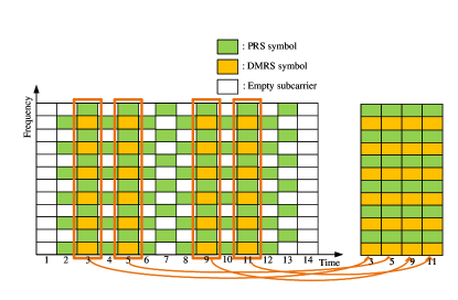
Figure 3: Joint DMRS and PRS time-frequency resource allocation scheme

Then, CSI-RS signal is inserted as shown in Fig. 4. It is revealed that the 2nd to 12th symbols in the odd-numbered subcarriers in a PRB are continuous and can be extracted for velocity estimation. Therefore, $K_{\rm{comb}}^{\rm{\rm{symbol}}}=1$.

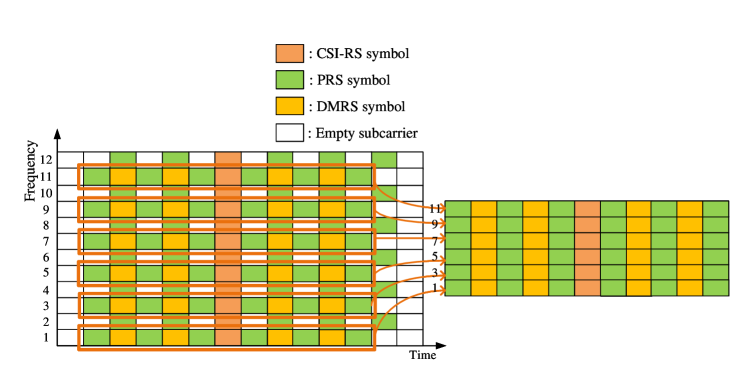
Figure 4: Joint DMRS, PRS and CSI-RS time-frequency domain resource allocation scheme

Based on the resource allocation scheme in time-frequency domain in Fig. 3 and Fig. 4, (9) is equivalent to

$$\small\mathbf{S}_{\rm{rx}}(k,m)=\xi\mathbf{S}_{\rm{tx}}(k,m)e^{j2\pi mT_{s}f_{d,r}}e^{-j2\pi k\Delta f\frac{2R}{c}}.$$ (12)

The signal processing framework is presented in Fig. 5. The reference signals generated by Gold sequence are mapped to the corresponding OFDM symbols according to the time-frequency mapping diagrams. After conventional OFDM modulation, transmission, target reflection, receiving, extracting continuous resources in the time or frequency domain, 2D-FFT algorithm is applied in the estimation of distance and velocity.

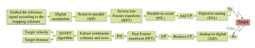
Figure 5: ISAC signal processing frame

IV Sensing Performance Analysis

In this section, the maximum unambiguous distance and velocity, the resolutions and CRLBs for distance and velocity estimation are derived in details.

2D-FFT algorithm removes the transmitted information in the received signal. Since signal processing in frequency domain is not affected by data signal, the randomness of time domain correlation processing using the communication signal is eliminated, benefiting the improvement of sensing performance [21]. With the 2D-FFT algorithm in [21], the signal processing for the proposed multiple reference signals collaborative sensing scheme is implemented.

Removing transmitted information from the received echo symbols by point-wise division, we have

$$\small(\mathbf{S}_{g})_{k,m}=\frac{\mathbf{S}_{\rm{rx}}(k,m)}{\mathbf{S}_{\rm{tx}}(k,m)}=\xi e^{j2\pi mT_{s}f_{d,r}}e^{-j2\pi k\Delta f\frac{2R}{c}}.$$ (13)

IV-A Resolution of Distance and Velocity Estimation

Performing IFFT on the $m$-th column of $\mathbf{S}_{g}$, we have

$$\small{\rm{IFFT}}(\mathbf{S}_{g,m}(k))=\sum_{k=0}^{N-1}e^{-j2\pi k\Delta f\frac{2R}{c}}\times e^{\frac{j2\pi rk}{N}}.$$ (14)

The index of peak is recorded as $ind_{s_{g},m}$, so that the estimated distance $\hat{R}$ is

$$\small\hat{R}=\frac{c\hat{r}}{2N\Delta f}=\frac{ind_{s_{g},m}c}{2N\Delta f},\quad ind_{s_{g},m}\in\{0,1,\ldots,N-1\}.$$ (15)

The maximum detection distance is

$$\small R_{max}=\frac{c}{2\Delta f}.$$ (16)

Compared to [12], the maximum unambiguous detection distance is enlarged by $K_{\rm{comb}}^{\rm{PRS}}$ times, where $K_{\rm{comb}}^{\rm{PRS}}\in\{2,4,6,12\}$ is the comb size of PRS.

The distance resolution is

$$\small\Delta R=\frac{c}{2N\Delta f}.$$ (17)

(16) and (17) reveal that $\Delta f$ is inversely proportional to the maximum measurable distance and the distance resolution. There is a trade-off between the maximum measurable distance and distance resolution when choosing $\Delta f$.

Performing FFT on the $k$-th row of $\mathbf{S}_{g}$, we have

$$\small{\rm{FFT}}(\mathbf{S}_{g,k}(m))=\sum_{m=0}^{M-1}e^{j2\pi mT_{s}f_{d,r}}\times e^{-\frac{j2\pi dm}{M}}.$$ (18)

The index of peak is recorded as $ind_{s_{g},k}$, so that the estimated Doppler frequency shift $\hat{f}_{d,r}$ is

$$\small\hat{f}_{d,r}=\frac{ind_{s_{g},k}}{MT_{s}}.$$ (19)

Because

$$\small v=\frac{cf_{d,r}}{2f_{c}},$$ (20)

the estimated velocity is

$$\small\hat{v}=\frac{ind_{s_{g},k}c}{2MT_{s}f_{c}},\quad ind_{s_{g},k}\in\{0,1,\ldots,M-1\}.$$ (21)

The maximum estimated velocity is

$$\small v_{max}=\frac{c}{2T_{s}f_{c}}.$$ (22)

Compared to [12], the maximum unambiguous measurable velocity is enlarged by $K_{\rm{comb}}^{\rm{PRS}}$ times.

The velocity resolution is

$$\small\Delta v=\frac{c}{2MT_{s}f_{c}}.$$ (23)

According to (22) and (23), the resolution in velocity estimation is improving when $T_{s}$ and $f_{c}$ are increasing at the cost of reducing the maximum measurable velocity. There is a trade-off between the maximum measurable velocity and velocity resolution when choosing $T_{s}$ and $f_{c}$.

IV-B CRLB of Distance and Velocity Estimation

Theorem 1.

The CRLBs of the proposed ISAC signal for distance and velocity estimation are as follows with the conditions $M\gg 1,N\gg 1$.

$$\small CRLB\left(R\right){\rm{=}}\frac{{{c^{2}}}}{{{\xi^{2}}\cdot\gamma\cdot{{({2\pi\Delta f})}^{2}}}}\cdot{\mkern 1.0mu}\frac{{12}}{{M_{J}N({N-1})({7N+1})}},$$ (24)

$$\small CRLB\left(v\right){\rm{=}}\frac{c^{2}}{{{\xi^{2}}\cdot\gamma\cdot{{({2\pi T_{s}})}^{2}}f_{c}}}\cdot\frac{{12}}{{N_{J}M({M-1})({7M+1})}},$$ (25)

with $\gamma=\frac{A^{2}}{\sigma^{2}}$ representing the signal-to-noise ratio (SNR).

Proof.

Considering the distance estimation, since the modulation symbol is known in radar receiver and the additive white Gaussian noise (AWGN) follows one-dimensional (1-D) Gaussian distribution, the receiving signal is written as

$$\small z_{m,n}=\xi A_{m,n}e^{j2\pi K_{\rm{comb}}^{\rm{symbol}}mT_{s}f_{d,r}}e^{-j2\pi n\Delta f\tau}+w_{m,n},$$ (26)

where $\xi$ is the attenuation factor during the target reflection process, which is a constant, $w_{m,n}$ is the AWGN following $N(0,\sigma^{2})$, and $A_{m,n}=\left|x_{m,n}\right|$ is the amplitude of modulation symbol. According to Fig. 3, $K_{\rm{comb}}^{\rm{symbol}}$ in this paper is not fixed. The four columns of multiple reference signal extracted is continuous in frequency domain, namely, $K_{\rm{comb}}^{\rm{carrier}}=1$, which can be omitted.

$z_{m,n}$ with unknown parameters $\theta=(\tau,f_{d,r})$ is observed. An estimation of $\theta$ is performed, whose likelihood function is

$$\small\begin{array}[]{l}f\left({\left.z\right|\tau,{f_{d,r}}}\right)=\frac{1}{{{{\left({2\pi{\sigma^{2}}}\right)}^{\frac{{MN}}{2}}}}}\cdot\\ {e^{-\frac{1}{{2{\sigma^{2}}}}\sum\limits_{m}{\sum\limits_{n}{{{\left|{{z_{m,n}}-\xi{A_{m,n}}{e^{j2\pi K_{{\rm{comb}}}^{{\rm{symbol}}}m{T_{s}}{f_{d,r}}}}{e^{-j2\pi n\Delta f\tau}}}\right|}^{2}}}}}}.\end{array}$$ (27)

The log-likelihood function is

$$\small\begin{array}[]{l}L\left({\left.z\right|\tau,{f_{d,r}}}\right){\rm{=}}\ln f\left({\left.z\right|\tau,{f_{d,r}}}\right)=-\frac{{MN}}{2}\ln\left({2\pi{\sigma^{2}}}\right)\\ -\frac{1}{{2{\sigma^{2}}}}\sum\limits_{m}{\sum\limits_{n}{{{\left|{{z_{m,n}}-\xi{A_{m,n}}{e^{j2\pi K_{{\rm{comb}}}^{{\rm{symbol}}}m{T_{s}}{f_{d,r}}}}{e^{-j2\pi n\Delta f\tau}}}\right|}^{2}}}}.\end{array}$$ (28)

Letting $s_{m,n}=\xi{A_{m,n}}{e^{j2\pi K_{{\rm{comb}}}^{{\rm{symbol}}}m{T_{s}}{f_{d,r}}}}{e^{-j2\pi n\Delta f\tau}}$, (28) can be simplified as

$$\small L=-\frac{{MN}}{2}\ln\left({2\pi{\sigma^{2}}}\right)-\frac{1}{{2{\sigma^{2}}}}\sum\limits_{m}{\sum\limits_{n}{{{\left|{{z_{m,n}}-{s_{m,n}}}\right|}^{2}}}}.$$ (29)

The Fisher information matrix $\mathbf{F}$ is

$$\small\begin{array}[]{l}\mathbf{F}{\rm{=}}\left[{\begin{array}[]{*{20}{c}}{{\mathbf{F}_{\tau\tau}}}&{{\mathbf{F}_{\tau{f_{d,r}}}}}\\ {{\mathbf{F}_{{f_{d,r}}\tau}}}&{{\mathbf{F}_{{f_{d,r}}{f_{d,r}}}}}\end{array}}\right]\\ =-\left[{\begin{array}[]{*{20}{c}}{E\left({\frac{{{\partial^{2}}L}}{{\partial{\tau^{2}}}}}\right)}&{E\left({\frac{{{\partial^{2}}L}}{{\partial\tau\partial{f_{d,r}}}}}\right)}\\ {E\left({\frac{{{\partial^{2}}L}}{{\partial{f_{d,r}}\partial\tau}}}\right)}&{E\left({\frac{{{\partial^{2}}L}}{{\partial{f_{d,r}}^{2}}}}\right)}\end{array}}\right].\end{array}$$ (30)

Since the CRLB matrix is the inverse of Fisher information matrix [12], the CRLB matrices of delay and Doppler frequency shift estimation are

$$\small\left[{\begin{array}[]{*{20}{c}}{CRLB\left(\tau\right)}&{CRLB\left({\tau,{f_{d,r}}}\right)}\\ {CRLB\left({{f_{d,r}},\tau}\right)}&{CRLB\left({{f_{d,r}}}\right)}\end{array}}\right]{\rm{=}}{\mathbf{F}^{-1}}.$$ (31)

Thus, we have

$$\small{\begin{array}[]{*{20}{l}}{CRLB\left(\tau\right){\rm{=}}\frac{{{\mathbf{F}_{{f_{d,r}}{f_{d,r}}}}}}{{{\mathbf{F}_{\tau\tau}}{\mathbf{F}_{{f_{d,r}}{f_{d,r}}}}-{\mathbf{F}_{\tau{f_{d,r}}}}{\mathbf{F}_{{f_{d,r}}\tau}}}}}.\end{array}}$$ (32)

For velocity estimation, the time of two symbols at the edge of a slot is very short, and the velocity changes very slowly, which can be regarded as continuous. Hence, the the receiving signal is expressed as

$$\small z_{m,n}=\xi A_{m,n}e^{j2\pi mT_{s}f_{d,r}}e^{-j2\pi K_{\rm{comb}}^{\rm{carrier}}n\Delta f\tau}+w_{m,n},$$ (33)

where the meanings of $\xi$, $A_{m,n}$ and $w_{m,n}$ are the same as those in (26). From Fig. 4, we have $K_{\rm{comb}}^{\rm{carrier}}=2$. The symbols of the multiple reference signals on the subcarriers with odd indexes can be approximately regarded as continuous, namely $K_{\rm{comb}}^{\rm{symbol}}=1$, which can be omitted.

Similarly, we have

$$\small\begin{array}[]{*{20}{l}}{CRLB\left({{f_{d,r}}}\right){\rm{=}}\frac{{{\mathbf{F}_{\tau\tau}}}}{{{\mathbf{F}_{\tau\tau}}{\mathbf{F}_{{f_{d,r}}{f_{d,r}}}}-{\mathbf{F}_{\tau{f_{d,r}}}}{\mathbf{F}_{{f_{d,r}}\tau}}}}}.\end{array}$$ (34)

As CRLB is minimum variance of the unbiased estimator, mathematics nature of CRLB is the same as that of variance. Therefore, the CRLBs for distance and velocity estimation are

$$\begin{split}\small CRLB(R)=\frac{{{c^{2}}}}{4}CRLB(\tau),\end{split}$$ (35)

$$\begin{split}\small CRLB(v)=\frac{{{c^{2}}}}{{4f_{c}^{2}}}CRLB({{f_{d,r}}}).\end{split}$$ (36)

∎

It is revealed that with $T_{s}$ decreasing, CRLB for distance estimation decreases, which is opposite to the CRLB for velocity estimation. For a specific application scenario, a tradeoff between velocity and distance estimation needs to be considered when selecting $T_{s}$.

V Improved Velocity Estimation Method

In order to improve the accuracy of velocity estimation on discontinuous resources, the CS is combined with 2D-FFT in this section.

As shown in Fig. 4, one or two OFDM symbols of the multiple reference signals are still discontinuous at the edge of a time slot, resulting in discontinuous row vectors of channel information matrix and high side lobe, which causes false alarm and weak echo signal.

The theory of CS indicates that for a sparse signal that can be mapped onto a low-dimensional space, the original signal can be reconstructed by solving a sparsity-constrained optimization problem [23]. The process of CS is shown in Fig. 6. If the original signal $\mathbf{e}$ is not sparse, it needs to be sparsely represented on a sparse basis. Let

$$\small\mathbf{e}=\mathbf{\Psi h},$$ (37)

where $\mathbf{\Psi}$ is a sparse basis matrix and $\mathbf{h}$ is sparse coefficient vector.

The observed $\mathbf{y}$ is obtained through the observation matrix $\mathbf{\Phi}$,

$$\small\mathbf{y}=\mathbf{\Phi\Psi h}.$$ (38)

The reconstruction problem of CS is to solve the underdetermined equation (38) to obtain $\mathbf{h}$ and $\mathbf{e}$, based on the known $\mathbf{y}$, $\mathbf{\Psi}$, and $\mathbf{\Phi}$.

The improved velocity estimation algorithm comes from the sparsity of target [24]. In the sensing algorithm, a target corresponds to single peak in the velocity profile, so that the echo signal is sparse in the velocity profile space, namely, the velocity profile $\mathbf{V}_{k}$ is compressible [25]. Therefore, $\mathbf{V}_{k}$ does not need to be sparsely represented, namely, Step 1 of Fig. 6 is omitted.

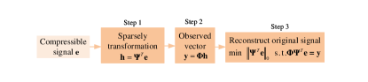
Figure 6: Compressed sensing framework

The discrete Fourier transform (DFT) of $\mathbf{k}_{v}$ in 2D-FFT algorithm is equivalent to multiplying the discrete Fourier matrix $\mathbf{\Gamma}$ to obtain $\mathbf{V}_{k}$,

$$\small\mathbf{V}_{k}=\mathbf{k}_{v}\mathbf{\Gamma}.$$ (39)

Then, we have

$$\small\mathbf{k}_{v}=\mathbf{V}_{k}\mathbf{\Gamma}^{-1}.$$ (40)

It is known that the discrete Fourier matrix is a partial Fourier random matrix [26], which satisfies the restricted isometric principle (RIP). The IDFT matrix also satisfies RIP and can be used as $\mathbf{\Phi}$ in Fig. 6. Then, (40) is equivalent to Step 2 in Fig. 6.

Therefore, the process of obtaining velocity profile matrix $\mathbf{V}_{k}$ from channel row vector $\mathbf{k}_{v}$ can be regarded as the problem of reconstructing the sparse signal, namely, Step 3 in Fig. 6. Thus $\mathbf{V}_{k}$ can be obtained by solving a sparse optimization problem. Since $l_{0}$ norm is not continuous, $l_{1}$ norm is used to replaced $l_{0}$ norm. Then the optimization problem is rewritten as

$$\small\hat{\mathbf{V}}_{k}={\rm{min}}{\|\mathbf{V}_{k}\|}_{1}\quad\mathbf{s.t.}{\|\mathbf{k}_{v}-\mathbf{V}_{k}\mathbf{\Gamma}^{-1}\|}_{2}\leq\varepsilon,$$ (41)

where ${\|\cdot\|}_{1}$ is $l_{1}$ norm, ${\|\cdot\|}_{2}$ is $l_{2}$ norm, $\varepsilon$ is the noise tolerance.

Overall, as a result of the sparsity of the velocity profile domain and the observation matrix satisfying RIP, the reconstruction model of CS is well suited for the velocity estimation in this paper. The specific implementation steps are introduced as follows.

Step 1: Since the linear displacement of the velocity only exists in time domain, each row of the channel matrix $\mathbf{S}_{g}$ is taken to get $\mathbf{k}_{v}$, creating the IDFT matrix $\mathbf{\Gamma}^{-1}$

$$\small\mathbf{\Gamma}^{-1}=\left[\begin{array}[]{ccccc}1&1&1&\cdots&1\\ 1&W_{N}^{-1}&W_{N}^{-2}&\cdots&W_{N}^{-(M-1)}\\ 1&W_{N}^{-2}&W_{N}^{-4}&\cdots&W_{N}^{-2(M-1)}\\ \vdots&\vdots&\vdots&\ddots&\vdots\\ 1&W_{N}^{-(M-1)}&W_{N}^{-2(M-1)}&\cdots&W_{N}^{-(M-1)(M-1)}\end{array}\right],$$ (42)

where $W_{N}=e^{j\frac{2\pi}{N}}$.

Step 2: Construct a zeroing matrix $\mathbf{A}$, which is used in zeroing the corresponding row of $\mathbf{S}_{g}$ and $\mathbf{\Gamma}^{-1}$. $\mathbf{A}=[a_{0},a_{1},\ldots,a_{M-1}]$, where $a_{m}\in\{0,1\}$. The value of $a_{m}$ is defined by whether there is channel information. If there is channel information, then $a_{m}=1$, otherwise $a_{m}=0$. For the odd-numbered and even-numbered rows of $\mathbf{S}_{g}$ and $\mathbf{\Gamma}^{-1}$, $\mathbf{A}$ is different. As shown in Fig. 7, for odd-numbered rows, $\mathbf{A}_{1}=[0111111111110001111111111100]$. For even-numbered rows, $\mathbf{A}_{2}=[0010101010101000101010101010]$. Setting zero by

$$\small\mathbf{k}_{v}^{\prime}=\left\{\begin{array}[]{l}\mathbf{k}_{vm}\circ\mathbf{A}_{1},\text{ when }m\text{ is an odd}\\ \mathbf{k}_{vm}\circ\mathbf{A}_{2},\text{ when }m\text{ is an even},\end{array}\right.$$ (43)

where $\circ$ is Hadamard product, $\mathbf{k}_{vm}$ is $m$-th row vector of $\mathbf{S}_{g}$. $(\mathbf{k}_{v}^{\prime})_{o}$ is obtained by deleting the empty element of $\mathbf{k}_{v}^{\prime}$. Then we perform the same operation on $\mathbf{\Gamma}^{-1}$ to obtain the observation matrix $(\mathbf{\Gamma}^{-1})^{\prime}_{o}$.

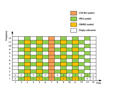
Figure 7: Zeroing matrix of different rows

Step 3: Using the FISTA algorithm [27], $(\mathbf{k}_{v}^{\prime})_{o}$ is solved to obtain $\mathbf{V}_{k}$. Set the maximum number of iterations $I_{max}$ and error threshold $E_{th}$, and the solution process of FISTA is shown in Algorithm 1, where $\rm p_{L}$ is proximal operator.

Algorithm 1 Velocity Estimation Algorithm based on FISTA

Sparse signal: $(\mathbf{k}_{v}^{\prime})_{o}$.

Observation matrix: $(\mathbf{\Gamma}^{-1})^{\prime}_{o}$.

Regularization parameter: $\lambda$.

Maximum number of iterations: $I_{max}$.

The threshold of iteration error: $E_{th}$.

i.e. $\mathbf{y}$, $\mathbf{\Phi}$, $\lambda$, $I_{max}$ and $E_{th}$.

$1\times M$ dimensional velocity profile matrix $\mathbf{V}_{k}$: $\mathbf{e}$.

while $err(i+1)-err(i)\geq E_{th}$ and ${\it i}\leq I_{max}$ do

     $\mathbf{p}_{1}=\vec{\mathbf{0}},t_{1}=1$;

     $\mathbf{e}_{i}=\operatorname{p_{L}}\left(\mathbf{p}_{i}\right)$;

     $t_{i+1}=\frac{1+\sqrt{1+4t_{i}^{2}}}{2}$;

     $\mathbf{p}_{i+1}=\mathbf{e}_{i}+\left(\frac{t_{i}-1}{t_{i+1}}\right)\left(\mathbf{e}_{i}-\mathbf{e}_{i-1}\right)$;

     $err(i+1)={\|\mathbf{\Phi}\mathbf{e}_{i}-\mathbf{y}\|}_{2}$;

end while

$err(i+1)-err(i)\textless E_{th}$.

Step 4: Accumulate and normalize $N$ velocity profile matrixes $\mathbf{V}_{k}$. Then, perform peak search on the velocity profile to obtain the index value $ind_{s_{g},k}$ of the peak value. Finally, (21) is applied to calculate the velocity of target.

VI Simulation Results and Analysis

The sensing performance of the multiple reference signals collaborative sensing scheme is verified in this section. 2D-FFT algorithm [21] is employed in distance and velocity estimation. The parameters in simulation are shown in Table II. 100 times Monte Carlo simulations are conducted for each simulation setting.

TABLE II: Simulation parameters

Symbol	Parameter	Value
$T_{\rm{sample}}$	Sampling interval	$0.016\ {\rm{\upmu s}}$
$T_{\rm{s}}$	Total OFDM symbol duration	$8.92\ {\rm{\upmu s}}$
$T_{\rm{cp}}$	Duration of CP	$0.57\ {\rm{\upmu s}}$
$T$	Duration of OFDM symbol	$8.33\ {\rm{\upmu s}}$
$\Delta f$	Subcarrier spacing	120 kHz
$f_{\rm{c}}$	Carrier frequency	24 GHz
$\gamma$	Signal to noise ratio	$\left[-15,10\right]\ \rm{dB}$
$N$	Number of subcarriers	256
$M$	Number of symbols	140/28

VI-A Distance Estimation

To show the sensing performance of the proposed multiple reference signals collaborative sensing scheme, a target with a relative distance of 48 m is detected. In the perspective of root mean square error (RMSE) and root CRLB, the distance estimation performance of different reference signals is compared. The effect of subcarrier spacing on distance estimation is investigated in this subsection.

Fig. 8 shows the spectrum diagram of echo signal for distance estimation, where $\rm index_{r}$ is the index when searching IFFT peak. Compared to low sidelobe, the target has extremely high peak amplitude. Referring to the analysis in Section IV, the estimated distance $\hat{R}=\frac{ind_{s_{g},m}c}{2N\Delta f}=48.83$ m.

For further performance evaluation, Fig. 9 demonstrates RMSE and root CRLB for distance estimation using PRS, DMRS, and joint PRS and DMRS over different SNR values. Compared with the single PRS or DMRS, joint PRS and DMRS significantly improves the accuracy of distance estimation with low SNR. RMSE of joint PRS and DMRS for distance estimation sharply declines when SNR is $-$15 dB and stabilizes to 0.83 m at the SNR of $-$9 dB, which is earlier than the single PRS or DMRS. It is discovered that RMSEs for distance estimation using PRS, DMRS, and joint PRS and DMRS stabilize to the same value. The reason is that the peak index of IFFT can only take integer, the distance of possible estimation is quantized on a regular grid, resulting in quantization errors [28]. The RMSE of joint PRS and DMRS scheme is approaching to the root CRLB when the SNR is increasing. Under the condition of about 30 MHz bandwidth, the accuracy of distance estimation is limited to approximately 0.83 m when SNR is larger than $-$9 dB.

As shown in Fig. 10, the RMSE of joint PRS and DMRS scheme for distance estimation with subcarrier spacing of 240 kHz and 30 kHz are 0.83 m and 6.75 m respectively when the SNR is larger than $-$8 dB. It is revealed that the error of distance estimation is decreasing with the decreasing of subcarrier spacing. The reason is that with the fixed number of subcarriers, the bandwidth increases with the increase of subcarrier spacing.

Fig. 11 reveals that the increase of subcarrier spacing decreases the root CRLB for distance estimation, which shows the same trend as RMSE. (35) can explain this downtrend clearly. It is also shown that the theoretically achievable accuracy of distance estimation with joint PRS and DMRS scheme is higher than that of the single PRS or DMRS, which means that joint PRS and DMRS scheme has better performance for distance estimation.

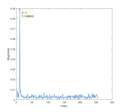
Figure 8: The distance estimation of the proposed ISAC signal

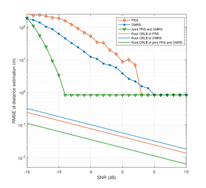
Figure 9: Comparison of RMSEs for distance estimations among PRS, DMRS, and joint PRS and DMRS

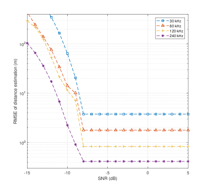
Figure 10: RMSE for distance estimation under different subcarrier spacing

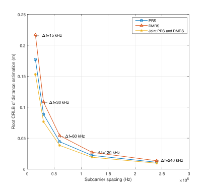
Figure 11: Root CRLB for distance estimation under different subcarrier spacing

VI-B Velocity Estimation

In this subsection, a target with relative velocity 18 m/s is detected. The RMSEs and root CRLBs of different reference signals for velocity estimation are presented. Then, the effects of carrier frequency and signal duration on velocity estimation are investigated.

RMSEs of the single reference signal and joint reference signals for velocity estimation are shown in Fig. 12. Due to the limitation of the minimum received SNR for radar detection, random and wrong detection result is obtained when the SNR is larger than $-$10 dB, making it meaningless to compare accuracy for velocity estimation of different signals. In the case of low SNR, RMSE of joint PRS, DMRS and CSI-RS is better than that of the single reference signal. The reason is that joint PRS, DMRS and CSI-RS inserts continuous and more symbols, so that it has a higher peak amplitude, which is more resistant to noise. RMSE for velocity estimation of joint PRS, DMRS and CSI-RS stabilizes earlier than the single reference signal, which stabilizes to 1.93 m/s when SNR is larger than $-$5 dB. With the increase of SNR, the RMSE of joint PRS and DMRS scheme is approaching to the root CRLB.

Fig. 13 shows the RMSE of joint PRS, DMRS and CSI-RS for velocity estimation when the carrier frequencies are 5.9 GHz and 24 GHz respectively. It is discovered that the velocity estimation at 24 GHz is better than that at 5.9 GHz. Combined with the analysis in Section IV, higher carrier frequency results in higher velocity resolution, further reducing RMSE of velocity estimation.

As shown in Fig. 14, RMSE of joint PRS, DMRS and CSI-RS scheme for velocity estimation with subcarrier duration of 4.46 ${\rm{\upmu s}}$ is 0.59 m/s when SNR is larger than $-$4 dB. It is revealed that increasing the signal duration can effectively reduce the error of velocity estimation.

Fig. 15 indicates that with the increase of signal duration, the root CRLB for velocity estimation increases, which shows the same trend as RMSE. The reason is that the minimum identifiable velocity unit by the system is reduced, thereby improving the accuracy of velocity estimation.

Fig. 16 illustrates the root CRLB for distance and velocity estimation with the joint reference signals under different subcarrier spacing. It is revealed that when the subcarrier spacing is increasing, the accuracy of distance estimation is enhancing, while the accuracy of velocity estimation is reducing. Combining the analysis of Fig. 11 and Fig. 15 and the inversely proportional relationship between the subcarrier spacing and the signal duration, the tradeoff relation between the distance and velocity estimation can be explained in Fig. 16. It is discovered that the root CRLBs for velocity estimation and distance estimation both decrease with the increase of SNR, which verified the derived results in (24) and (25).

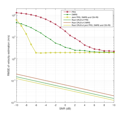
Figure 12: Comparison of RMSEs for velocity estimations among PRS, DMRS and the joint signal

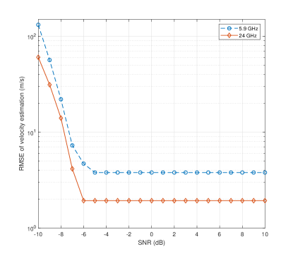
Figure 13: RMSE for velocity estimation at different carrier frequencies

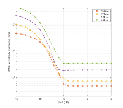
Figure 14: RMSE for velocity estimation under different signal duration

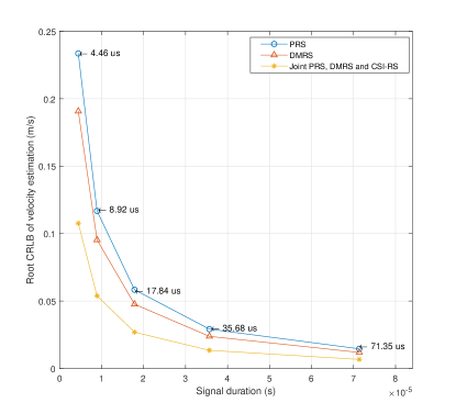
Figure 15: Root CRLB for velocity estimation under different signal duration

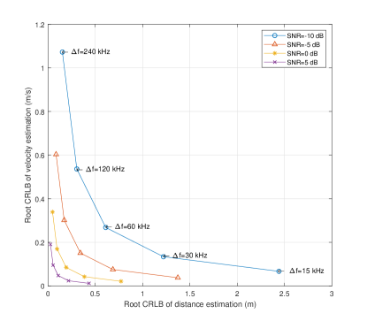
Figure 16: The relationship between CRLB for distance and velocity estimation

VI-C Improved Velocity Estimation Algorithm using CS

The performance of velocity estimation using the improved 2D-FFT algorithm in Section V is simulated and compared with traditional 2D-FFT algorithm, where detecting a target of a relative velocity of 25 m/s with only 28 symbols is simulated.

The spectrum diagrams of the echo signal with 2D-FFT algorithm and the improved 2D-FFT algorithm using CS are shown in Fig. 17, where $\rm index_{v}$ is the index when searching FFT peak. It is obvious that CS improves the peak-to-sidelobe level ratio (PSLR) of velocity spectrogram from 1.86 to 5.15, which enhances the capability of ISAC system to resist noise and clutter. RMSEs for velocity estimation with the two algorithms are shown in Fig. 18. The improved 2D-FFT algorithm only occupies 28 symbols, whose RMSE for velocity estimation is stable to 1.79 m/s when the SNR is larger than $-$20 dB, while the RMSE for velocity estimation with the traditional 2D-FFT algorithm is stable when the SNR is larger than 0 dB. When SNR is in the range of $-$20 to 0 dB, the improved 2D-FFT algorithm has much better sensing performance than the traditional 2D-FFT algorithm.

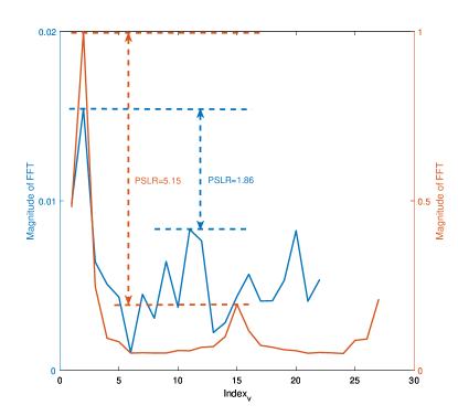
Figure 17: The velocity estimation with 2D-FFT algorithm and 2D-FFT algorithm using CS

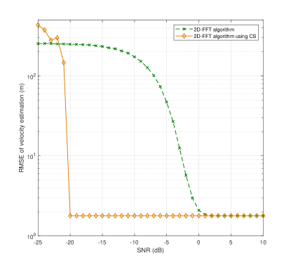
Figure 18: Comparison of RMSEs with the two algorithms for velocity estimation

VII Conclusion

The multiple reference signals in 5G NR standard are collaboratively applied in radar sensing. The time-frequency domain resources of DMRS, PRS, and CSI-RS are skillfully configured so that the multiple reference signals continuously distribute in the time and frequency domain to obtain good sensing performance. According to the analysis of sensing performance, the CRLBs of the proposed ISAC signal on distance and velocity estimation have a tradeoff relation. Besides, an improved 2D-FFT algorithm based on CS is designed for velocity estimation, which overcomes the limitation of 2D-FFT algorithm on discontinuous signals in time domain and improves the ability to resist noise and clutter. In the end, we verified that the joint reference signals, instead of single reference signal, have better potential to be applied in radar sensing, which is a practical and efficient approach in designing ISAC signal towards 5G-A and 6G.

References

- [1] X. Duan, L. Yang, S. Xia, Z. Han, F. Xie. “Technology development mode of communication/sensing/computing/intelligence integration," Telecommunications Science , 2022, 38(3): 37-48.
- [2] H. Nie, F. Zhang, Y. Yang and S. Pan, “Photonics-based integrated communication and radar system," 2019 International Topical Meeting on Microwave Photonics (MWP), 2019, pp. 1-4, doi: 10.1109/MWP.2019.8892218.
- [3] Q. Ma, J. Lu and Y. Maoxiang, “Integrated Waveform Design For 64QAM-LFM Radar Communication," 2021 IEEE 5th Advanced Information Technology, Electronic and Automation Control Conference (IAEAC), 2021, pp. 1615-1625, doi: 10.1109/IAEAC50856.2021.9390784.
- [4] F. Liu, L. Zhou, C. Masouros, A. Li, W. Luo and A. Petropulu, “Toward Dual-functional Radar-Communication Systems: Optimal Waveform Design," in IEEE Transactions on Signal Processing, vol. 66, no. 16, pp. 4264-4279, 15 Aug. 15, 2018, doi: 10.1109/TSP.2018.2847648.
- [5] X. Liu, T. Huang, N. Shlezinger, Y. Liu, J. Zhou and YC Eldar, “Joint Transmit Beamforming for Multiuser MIMO Communications and MIMO Radar," in IEEE Transactions on Signal Processing, vol. 68, pp. 3929 -3944, 2020, doi: 10.1109/TSP.2020.3004739.
- [6] D. Ma, LIU X. Liu, T. Huang, et al. “Joint radar and communications: Shared waveform designs and performance bounds," Journal of Radars, 2022, 11(2): 198–212. doi: 10.12000/JR21146
- [7] Y. Liu, G. Liao, Z. Yang, J. Xu. “A Super-resolution Design Method for Integration of OFDM Radar and Communication," Journal of Electronics & Information Technology, 2016, 38(2): 425-433. doi: 10.11999/JEIT150320
- [8] X. Wang, Z. Zhang. “Waveform Optimization Design for Integration of Radar and Communication Based on Multi-symbol OFDM," Electronics Optics & Control, 2021, 28(7): 83. DOI:10.3969/j.issn.1671-637X.2021.07.017.
- [9] P. Yong, J. Wang, J. Ge. “A Novel Side-Lobe Suppression Technology for the OFDM-Based Joint Radar and Communication Waveforms Using the Mismatching," JOURNAL OF SIGNAL PROCESSING, 2020, 36(10): 1698-1707. doi: 10.16798/j.issn.1003-0530.2020.10.009
- [10] HUANG T, ZHAO T. “Low PMEPR OFDM Radar Waveform Design Using the Iterative Least Squares Algorithm," IEEE Signal Processing Letters, 2015, 22(11): 1975–1979. DOI: 10.1109/LSP.2015.2449305.
- [11] Z. Feng, Z. Fang, Z. Wei, X. Chen, Z. Quan and D. Ji, “Joint radar and communication: A survey," in China Communications, vol. 17, no. 1, pp. 1-27, Jan. 2020, doi: 10.23919/JCC.2020.01.001.
- [12] Z. Wei et al., “5G PRS-Based Sensing: A Sensing Reference Signal Approach for Joint Sensing and Communication System," in IEEE Transactions on Vehicular Technology, 2022, doi: 10.1109/TVT.2022.3215159.
- [13] Ma L, Pan C, Wang Q, et al. “A Downlink Pilot Based Signal Processing Method for Integrated Sensing and Communication Towards 6G," in 2022 IEEE 95th Vehicular Technology Conference:(VTC2022-Spring). IEEE, 2022: 1-5.
- [14] Ye H, Yu X, Ci N, et al. “Novel Method of Range and Velocity Measurement Based on OFDM Pilot Signal," 2017.
- [15] D. Bao, G. Qin and Y. Dong, “A Superimposed Pilot-Based Integrated Radar and Communication System," in IEEE Access, vol. 8, pp. 11520-11533, 2020, doi: 10.1109/ACCESS.2020.2965153.
- [16] C. D. Ozkaptan, E. Ekici, O. Altintas and C. -H. Wang, “OFDM Pilot-Based Radar for Joint Vehicular Communication and Radar Systems," in 2018 IEEE Vehicular Networking Conference (VNC), 2018, pp. 1-8, doi: 10.1109/VNC.2018.8628347.
- [17] O. Kanhere, S. Goyal, M. Beluri and T. S. Rappaport, “Target Localization using Bistatic and Multistatic Radar with 5G NR Waveform," in 2021 IEEE 93rd Vehicular Technology Conference (VTC2021-Spring), 2021, pp. 1-7, doi: 10.1109/VTC2021-Spring51267.2021.9449071.
- [18] M. L. Rahman, P. -f. Cui, J. A. Zhang, X. Huang, Y. J. Guo and Z. Lu, “Joint Communication and Radar Sensing in 5G Mobile Network by Compressive Sensing," in 2019 19th International Symposium on Communications and Information Technologies (ISCIT), 2019, pp. 599-604, doi: 10.1109/ISCIT.2019.8905229.
- [19] G. Hakobyan, M. Ulrich and B. Yang, “OFDM-MIMO Radar With Optimized Nonequidistant Subcarrier Interleaving," in IEEE Transactions on Aerospace and Electronic Systems, vol. 56, no. 1, pp. 572-584, Feb. 2020, doi: 10.1109/TAES.2019.2920044.
- [20] ETSI TS 138 211-2021,5G; NR; Physical channels and modulation (V16.5.0; 3GPP TS 38.211 version 16.5.0 Release 16)[S].
- [21] C. Sturm and W. Wiesbeck, “Waveform Design and Signal Processing Aspects for Fusion of Wireless Communications and Radar Sensing," in Proceedings of the IEEE, vol. 99, no. 7, pp. 1236-1259, July 2011, doi: 10.1109/JPROC.2011.2131110.
- [22] Kay S M. Fundamentals of statistical signal processing: estimation theory[M]. Prentice-Hall, Inc., 1993.
- [23] Donoho D L. “Compressed sensing," IEEE Transactions on information theory, 2006, 52(4): 1289-1306.
- [24] KNILL C, SCHWEIZER B, SPARRER S, et al. “High Range and Doppler Resolution by Application of Compressed Sensing Using Low Baseband Bandwidth OFDM Radar," IEEE Transactions on Microwave Theory and Techniques, 2018, 66(7): 3535- 3546. DOI: 10.1109/TMTT.2018.2830389.
- [25] Candès E J. “Compressive sampling," in Proceedings of the international congress of mathematicians, 2006, 3: 1433-1452.
- [26] Iwen M A. “Simple deterministically constructible rip matrices with sublinear fourier sampling requirements," in 2009 43rd Annual Conference on Information Sciences and Systems, IEEE, 2009: 870-875.
- [27] Zhang L, Xu G, Xue Q, et al. “An iterative thresholding algorithm for the inverse problem of electrical resistance tomography," Flow Measurement and Instrumentation, 2013, 33: 244-250.
- [28] Braun K M. OFDM radar algorithms in mobile communication networks[D]. Karlsruhe, Karlsruher Institut für Technologie (KIT), Diss., 2014, 2014.