MMT/Binospec Spectroscopic Survey of Two $z$ $\sim$ 0.8 Galaxy Clusters in the Eye of Horus Field

Abstract

The discovery of the Eye of Horus (EoH), a rare double source-plane lens system ($z_{\rm lens}$ $=$ 0.795; $z_{\rm src}$ $=$  1.302 and 1.988), has also led to the identification of two high-redshift ($z_{\rm phot}$ $\sim$ 0.8) galaxy clusters in the same field based on the subsequent analysis of the Subaru/Hyper Suprime-Cam (HSC) optical and XMM-Newton X-ray data. The two brightest cluster galaxies (BCGs), one of which is the lensing galaxy of the EoH, are separated by only $\sim$100″ ($=$ 0.75 Mpc $<$ $r_{200}$) on the sky, raising the possibility that these two clusters may be physically associated. Here, we present a follow-up optical spectroscopic survey of this EoH field, obtaining 218 secure redshifts using MMT/Binospec. We have confirmed that there indeed exist two massive ($M_{\rm dyn}$ $>$ $10^{14}$  M_☉) clusters of galaxies at $z$ $=$ 0.795 (the main cluster) and at $z=0.769$ (the NE cluster). However, these clusters have a velocity offset of $\sim$4300 km s^-1, suggesting that this two-cluster system is likely a line-of-sight projection rather than a physically-related association (e.g., a cluster merger). In terms of the properties of the cluster-member galaxies, these two $z\sim 0.8$ clusters appear well-developed, each harboring an old (age $=$ 3.6–6.0 Gyr) and massive ($M_{\mathrm{*}}$ $=$ 4.2–9.5 $\times$ $10^{11}$  M_☉) BCG and exhibiting a well-established red sequence (RS). This study underscores the importance of conducting a spectroscopic follow-up for high-redshift cluster candidates because RS-based cluster selections are susceptible to such a projection effect in general.

1 Introduction

Clusters of galaxies are important laboratories for cosmological studies. Observations of galaxy clusters at high redshifts (with an accurate mass calibration) produce valuable cosmological constraints (Mantz et al., 2010; Kravtsov & Borgani, 2012), allowing us to test cosmological models such as the now standard $\Lambda$CDM model. We can also investigate physical processes driving the evolution of clusters and their member galaxies as well as probing the nature of dark energy and dark matter (Allen et al., 2011; Kravtsov & Borgani, 2012).

Clusters of galaxies can be identified at a variety of wavelengths. In the X-ray, they show up as bright extended sources because hot plasma in the intracluster medium (ICM) emits strong bremsstrahlung radiation. In the optical and near-infrared, clusters can be identified as over-densities of evolved red galaxies through the detection of the so-called cluster red sequence (RS), and a number of such cluster-finding algorithms exist, such as the CAMIRA algorithm (Oguri, 2014; Oguri et al., 2018) applied to the HSC Subaru Strategic Program (Aihara et al., 2018). At millimeter wavelengths, the spectral distortion of the cosmic microwave background due to the inverse-Compton scattering by the ICM provides a nearly redshift-independent signal for a given cluster mass, i.e. Sunyaev-Zel’dovich effect (SZ effect; Sunyaev & Zeldovich, 1972), and this effect has been exploited by the Atacama Cosmology Telescope (ACT; Hasselfield et al., 2013) and South Pole Telescope SZ surveys (Reichardt et al., 2013; Bleem et al., 2015).

The “Eye of Horus” (HSC J142449-005322; $\text{RA}=14^{\mathrm{h}}24^{\mathrm{m}}49^{\mathrm{s}}.0$ and $\text{Dec}=-0^{\circ}53^{\prime}21^{\prime\prime}.7$, J2000; hereafter EoH) is a strong gravitational lens system discovered through the HSC Subaru Strategic Program (Tanaka et al., 2016). In this system, one foreground galaxy at $z_{\mathrm{lens}}=0.795$ is gravitationally lensing two distant background galaxies at $z_{\mathrm{src}}=1.988$ and $z_{\mathrm{src}}=1.302$, and thus it is called a double source plane (DSP) system. Such a DSP system is rare because it requires two background galaxies at different redshifts and a lensing galaxy perfectly aligned along the light of sight. As a result, only a handful of DSP systems have been discovered so far (e.g., Gavazzi et al., 2008; Tu et al., 2009).

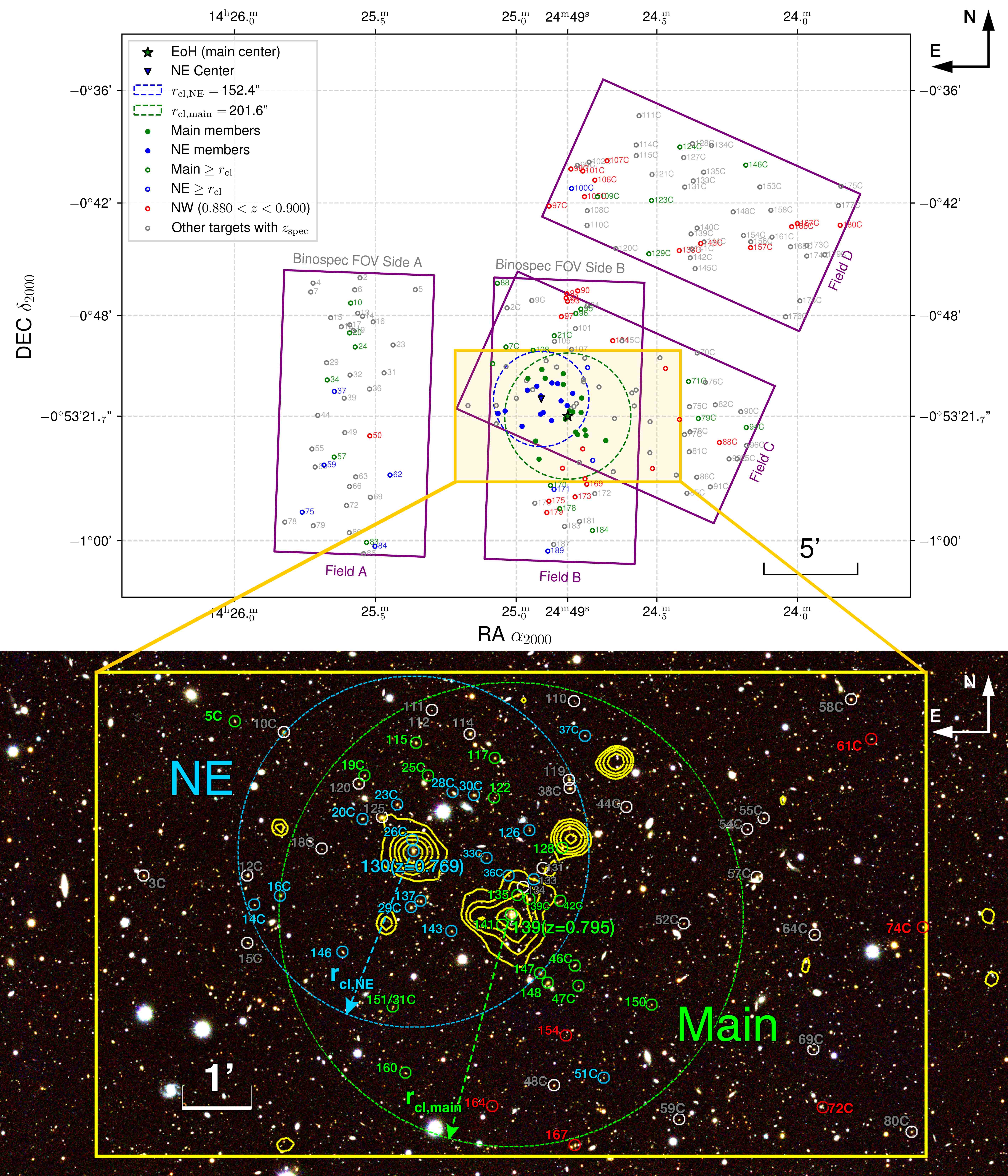
Figure 1: Positions of the main and NE cluster members. Upper panel — The MMT/Binospec field-of-views (FoVs) are denoted as Fields A–D, consisting of two mask designs of Side A+B for Run #1 (Fields A and B; PA $=$ $-2^{\circ}$) and #2 (Fields C and D; PA $=$ 66^∘), respectively. The member galaxies of the NE and main clusters are indicated with blue and green circles, respectively, while the blue triangle and green star indicate corresponding cluster BCGs. The green and blue dashed circles represent the virialized core radii $r_{\mathrm{cl}}$ ($r_{\mathrm{cl,main}}=201.6^{\prime\prime}$ and $r_{\mathrm{cl,NE}}=152.4^{\prime\prime}$). Lower panel — Spatial distribution of the MMT/Binospec-observed galaxies with slit numbers. The background is the three-color Subaru/HSC image with the r, i, z bands, and the yellow contours show the XMM-Newton X-ray map. The color definition is the same as the upper panel.

To better understand the surrounding structure that could potentially affect the lensing potential of this system, the environment of EoH was examined for the existence of any mass concentration. Recent studies based on the CAMIRA cluster catalog (Oguri et al., 2018) reported that two major clusters are located in the field of EoH with photometric redshifts of $z_{\mathrm{phot}}\sim 0.8$, which was subsequently confirmed by the XMM-Newton observation by Tanaka et al. (2020), hereafter referred to as T20, detecting X-ray emission that peaks at the locations of the two brightest cluster galaxies (BCGs) determined by CAMIRA. One of the X-ray emission peaks is at the lensing galaxy of EoH while the other peak is at the location of the galaxy SDSS J142454.68-005226.3 ($\text{RA}=14^{\mathrm{h}}24^{\mathrm{m}}54^{\mathrm{s}}.7$, $\text{Dec}=-0^{\circ}52^{\prime}26^{\prime\prime}.9$, J2000), which is positioned only $\sim 100$″ northeast (NE). The positions of the EoH lensing-galaxy BCG and second BCG are regarded as the centers of the corresponding galaxy clusters, denoted as the main and NE clusters, respectively, by T20. Their photometric redshifts suggest that the main and NE galaxy clusters are both at $z\sim 0.8$. Since their separation is only $\sim$ 100″ on the sky, one question arises: are they physically related (e.g., a cluster merger) or the superposition of two structures along the line of sight? Spectroscopic information is needed to confirm the existence of the two $z_{\mathrm{photo}}\sim 0.8$ clusters in this field and investigate their relationship. Although T20 hinted that this system is probably not a cluster merger due to the absence of X-ray emission between the two cluster peaks, it is not possible to provide a definitive answer without having spectroscopic data.

In this work, we utilized the Binospec multi-object spectrograph on the MMT telescope to answer the question above by presenting the results from our spectroscopic survey of two $z\sim 0.8$ clusters of galaxies conducted in the EoH field. We organized the paper by introducing the observational method in Section 2, presenting the results from our MMT/Binospec redshift survey in Section 3, and discussing cluster dynamical-mass estimates and the analysis of two BCG optical spectra in Section 4. Our conclusions are placed in Section 5. This paper uses standard $\Lambda$CDM cosmological parameters: $H_{0}=100h=70\,\mathrm{km}\,\mathrm{s}^{-1}\mathrm{Mpc}^{-1}$, $\Omega_{\mathrm{m}}=0.3$, and $\Omega_{\Lambda}=0.7$.

2 Observations and Data Reduction

2.1 MMT/Binospec

We used Binospec (Fabricant et al., 2019), a high-throughput imaging spectrograph with two $8^{\prime}\times 15^{\prime}$ fields of view (Side A and B) at the f/5 focus of the 6.5m MMT telescope, to conduct our redshift survey. The main spectral line features we look for are the Ca H&K ${\lambda}{\lambda}3933,3968$ absorption lines. For star-forming galaxies, we should also detect the [O II] ${\lambda}{\lambda}3727,3729$ emission lines. Continuum features like the Balmer and 4000 Å  breaks may also be detectable in the spectra. To achieve the best sensitivity at $\lambda\sim 7000-7600$ Å, where all these features appear at $z\sim 0.8$, we used the 600 lines/mm grating and set the central wavelength to 7300 Å, which results in a dispersion of 0.61 Å/pixel. Each slit has a $1^{\prime\prime}$ width corresponding to 3.32 pixels, producing a spectral resolution of $\Delta\lambda\sim 2$ Å. The resultant spectral resolving power is $R=3650$ at 7300 Å, high enough to clearly separate the Ca H&K lines.

The observations were executed on two dates: UT 2019 July 8 (Run #1; Field A and B) and UT 2022 January 31 (Run #2; Field C and D). For each run, we took 4 exposures of 1200 seconds each with a total integration time of 4800 seconds. The seeing varied between $1.2^{\prime\prime}$ and $1.3^{\prime\prime}$. We placed one of the $8^{\prime}\times 15^{\prime}$ field-of-views on top of the EoH field (Field B and C as shown in Figure 1). Binospec’s one field-of-view is large enough to contain the two targeted $z\sim 0.8$ galaxy clusters. With the minimum slit length of $\sim 8^{\prime\prime}$, we were able to target a few tens of cluster-member candidates with one slitmask. All the data have been processed by the standard Binospec data processing pipeline.

2.2 Target Selection

Run #1: Using the CAMIRA cluster catalog (S18A-Wide-v4), we first selected galaxies that were identified as the members of the main cluster at $z_{\rm CAMIRA}$ $=$ 0.79. These galaxies constitute our primary targets. Note, however, that the CAMIRA catalog only includes red galaxies that form the cluster RS. To recover cluster-member galaxies with bluer colors (e.g., due to star formation), we also used the original HSC Wide S18A source catalog and selected galaxies with photometric redshifts of $z$ $\sim$ 0.8$\pm$0.5 without applying any other color selection. This constitutes our secondary targets. In each target group, we assigned higher priorities to more massive (and therefore generally more luminous) galaxies based on the stellar masses provided by the CAMIRA catalog. The two BCGs were specifically targeted.

Run #2: For the 2nd run, we used an updated CAMIRA catalog (S20A-Wide-v2). We used the same target selection procedure as described above. The HSC Wide S18A source catalog was also used to select bluer cluster members. For this run, we adjusted the Binospec position angle (PA) such that the parallel field (Field D) will contain another high-redshift CAMIRA cluster candidate at $z_{\rm CAMIRA}$ $=$ 0.896.

In total, we targeted $\sim$400 galaxies in the EoH field containing two clusters of galaxies at $z\sim 0.8$ as identified by T20. Among the CAMIRA cluster-member candidates at $z_{\mathrm{CAMIRA}}=0.790,0.759$, and $0.896$ of 131, 105, and 32 galaxies, we observed 32, 39, and 13 galaxies in the two runs, which yields the Binospec-observed fraction of 24, 37, and 41% respectively.

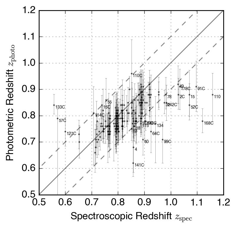
Figure 2: Spectroscopic vs. photometric redshifts. We used the photometric redshifts given by HSC/Mizuki (Tanaka, 2015; Tanaka et al., 2018). The majority (84%) of measured redshifts fall within the $\Delta z\leq 0.1$ region, marked with the dashed lines centered with the identity line (in solid). Galaxies with $\Delta z>0.1$ are additionally marked with their slit numbers. The scatter along the identity line is $\Delta(z_{\rm photo}-z_{\rm spec})/(1+z_{\rm spec})=0.07$

2.3 Redshift Measurements

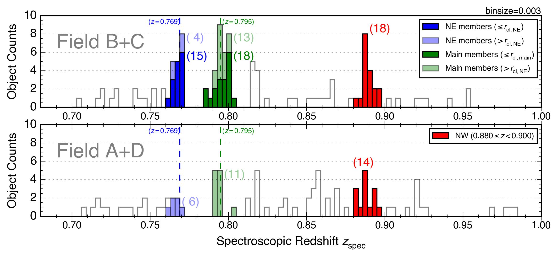
Figure 3: Redshift distributions of galaxies at $z$ $\sim$ 0.7–1.0 in the B and C fields (Upper Panel) and in the A and D fields (Lower Panel). The main and NE cluster members inside the virialized core radii $r_{\mathrm{cl}}$ are marked with deep green and blue, respectively. The numbers of the main and NE cluster members within $r_{\mathrm{cl}}$ are shown in deeper colors. Galaxy members selected by the shifting gapper method but outside $r_{\mathrm{cl}}$ are marked in light green and blue. The galaxies at $0.880\leq z<0.900$ (the redshift-range of the NW-cluster candidate) are shown in red. The white bins show other galaxies with $z_{\mathrm{spec}}$. The vertical dashed lines indicate the redshifts of the cluster BCGs, which we also take as the redshifts of their host clusters (i.e. main: $z=0.795$; NE: $z=0.769$).

To measure redshifts, we used SpecPro (Masters & Capak, 2011) software, which uses 19 galaxy templates with emission and absorption features. SpecPro has been adopted by the MMT observatory to analyze pipeline-processed Binospec 1D and 2D spectra, and for each manually-selected spectral template, it calculates multiple feasible redshift solutions. By following the procedure given by Shah et al. (2020), the most likely redshift solution was selected through visual inspection.

For each redshift determination, we assigned the “confidence” flag, indicating the reliability of the redshift measurement (3 = secure, 2 = likely, and 1 = no determination), which mainly depends on the signal-to-noise ratio of the spectrum being inspected. We record remarks and their issues in the “notes” column of Table 5.

3 Results

3.1 Spectroscopic Redshifts

All the measured spectroscopic redshifts are presented in Table 5. With the Run #1 observation, we observed 190 sources, which produced the redshift confidence-flag distribution of 56, 1, and 43% for 3, 2, and 1, respectively. With the Run #2 observation, we observed 181 sources with a confidence-flag distribution of 61, 3, and 36%. For our analyses, we only used spectra with a confidence flag of 3 or 2. In total, 221 secure redshifts were used in the following results and analysis. This includes 23, 28, and 6 secure redshifts from targets in the CAMIRA red candidate catalogs at $z_{\mathrm{CAMIRA}}=0.790,0.759$, and $0.896$, with the success rate (secure redshifts versus targeted) of 72, 72, and 46%.

Figure 2 compares the measured spectroscopic redshifts with the HSC-derived photometric redshifts, which were used for the target selection. The agreement is good with with $\Delta(z_{\rm photo}-z_{\rm spec})/(1+z_{\rm spec})=0.07$.

Figure 3 displays the redshift distribution for all the targets in both the Run #1 and #2 data. The Binospec spectral resolving power of $R=3650$ yields a redshift measurement uncertainty of $\Delta z=(1+z_{\rm spec})/R=0.0005$. We set the binsize of the redshift distribution histogram to 0.003, which is $6\Delta z$.

The spectroscopic redshift of the main-cluster BCG (Slit #139) is determined as $z_{\mathrm{main}}=0.795$ and that of the NE-cluster BCG (Slit #130) is $z_{\mathrm{NE}}=0.769$. We regard the locations of these two BCGs as the centers of the two clusters and treat these BCG redshifts as those of the respective clusters.

Table 1: Member Galaxies of the Main and NE Clusters

	NE BCG: Slit #130, ($\alpha$, $\delta$) $=$ (216.22772∘, -0.87414∘)							Main BCG: Slit #139, ($\alpha$, $\delta$) $=$  (216.20415∘, $-0.88935^{\circ}$)
	Slit #	$z$	$|v|$	$\Delta$RA	$\Delta$DEC	$r$		Slit #	$z$	$|v|$	$\Delta$RA	$\Delta$DEC	$r$
			( km s-1)	(′′)	(′′)	(′′)				( km s-1)	(′′)	(′′)	(′′)
1	130 ∙	$0.769$	$0$	$0$	$0$	$0$		139 ∙	$0.795$	$0$	$0$	$0$	$0$
2	26C ∙	$0.770$	$170$	$1$	$10$	$10$		141 ∙	$0.801$	$1003$	$8$	$-9$	$12$
3	23C ∙	$0.764$	$848$	$14$	$41$	$43$		135 ∙	$0.803$	$1337$	$-5$	$17$	$17$
4	137 ∙	$0.768$	$170$	$-6$	$-43$	$44$		39C ∙	$0.800$	$836$	$-16$	$13$	$21$
5	29C ∙	$0.764$	$848$	$2$	$-48$	$48$		42C ∙	$0.801$	$1003$	$-43$	$12$	$44$
6	20C ∙	$0.760$	$1526$	$44$	$28$	$52$		147 ∙	$0.790$	$836$	$-25$	$-51$	$57$
7	28C ∙	$0.765$	$678$	$-34$	$51$	$62$		148 ∙	$0.789$	$1003$	$-32$	$-59$	$67$
8	33C ∙	$0.766$	$509$	$-63$	$-6$	$64$		46C ∙	$0.786$	$1504$	$-55$	$-44$	$71$
9	30C ∙	$0.770$	$170$	$-52$	$49$	$72$		128 ∙	$0.799$	$669$	$-44$	$58$	$73$
10	143 ∙	$0.771$	$339$	$-33$	$-69$	$77$		47C ∙	$0.793$	$334$	$-58$	$-62$	$85$
11	36C ∙	$0.767$	$339$	$-83$	$-21$	$85$		122 ∙	$0.801$	$1003$	$15$	$101$	$102$
12	126 ∙	$0.767$	$339$	$-101$	$18$	$102$		151 ∙	$0.797$	$334$	$103$	$-80$	$130$
13	146 ∙	$0.766$	$509$	$61$	$-87$	$107$		117 ∙	$0.799$	$669$	$14$	$136$	$137$
14	16C ∙	$0.770$	$170$	$116$	$-38$	$122$		25C ∙	$0.793$	$334$	$72$	$121$	$141$
15	14C ∘	$0.770$	$170$	$138$	$-46$	$146$		150 ∙	$0.797$	$334$	$-122$	$-78$	$144$
16	37C	$0.770$	$170$	$-148$	$100$	$179$		160 ∙	$0.791$	$669$	$92$	$-138$	$165$
17	51C	$0.764$	$848$	$-165$	$-196$	$256$		115 ∘	$0.797$	$334$	$83$	$149$	$170$
18	171	$0.765$	$678$	$-41$	$-289$	$292$		19C ∘	$0.784$	$1838$	$127$	$120$	$175$
19	189	$0.770$	$170$	$-21$	$-486$	$487$		170	$0.798$	$501$	$55$	$-221$	$228$
20	62	$0.766$	$509$	$483$	$-243$	$541$		108	$0.796$	$167$	$111$	$210$	$238$
21	37	$0.765$	$678$	$662$	$24$	$662$		21C	$0.795$	$0$	$43$	$257$	$261$
22	100C	$0.770$	$170$	$-97$	$673$	$680$		5C	$0.801$	$1003$	$240$	$168$	$293$
23	84	$0.763$	$1018$	$532$	$-471$	$710$		7C	$0.798$	$501$	$198$	$221$	$297$
24	59	$0.761$	$1357$	$694$	$-211$	$726$		178	$0.791$	$669$	$25$	$-296$	$297$
25	75	$0.766$	$509$	$764$	$-362$	$845$		96	$0.795$	$0$	$-26$	$328$	$329$
26	-	-	-	-	-	-		95	$0.791$	$669$	$-42$	$342$	$345$
27	-	-	-	-	-	-		184	$0.795$	$0$	$-79$	$-366$	$374$
28	-	-	-	-	-	-		71C	$0.799$	$669$	$-386$	$110$	$402$
29	-	-	-	-	-	-		79C	$0.794$	$167$	$-417$	$-8$	$417$
30	-	-	-	-	-	-		88	$0.794$	$167$	$225$	$425$	$481$
31	-	-	-	-	-	-		94C	$0.795$	$0$	$-570$	$-36$	$572$
32	-	-	-	-	-	-		129C	$0.791$	$669$	$-259$	$519$	$580$
33	-	-	-	-	-	-		109C	$0.791$	$669$	$-95$	$701$	$707$
34	-	-	-	-	-	-		24	$0.794$	$167$	$679$	$221$	$714$
35	-	-	-	-	-	-		123C	$0.792$	$501$	$-268$	$689$	$739$
36	-	-	-	-	-	-		20	$0.803$	$1337$	$698$	$266$	$747$
37	-	-	-	-	-	-		57	$0.792$	$501$	$747$	$-131$	$758$
38	-	-	-	-	-	-		83	$0.795$	$0$	$643$	$-404$	$759$
39	-	-	-	-	-	-		34	$0.793$	$334$	$769$	$116$	$777$
40	-	-	-	-	-	-		10	$0.795$	$0$	$694$	$361$	$782$
41	-	-	-	-	-	-		124C	$0.791$	$669$	$-358$	$860$	$932$
42	-	-	-	-	-	-		146C	$0.793$	$334$	$-569$	$802$	$984$

Note. — $\bullet$ $r_{200}$–enclosed cluster members ($r\leq r_{200}$): $r_{200,\text{NE}}=127^{\prime\prime}=940$ kpc, $r_{200,\text{main}}=168^{\prime\prime}=1259$ kpc; $\circ$ Members outside $r_{200}$ but enclosed by the virialized core radii: $r_{200}<r\leq r_{\mathrm{cl}}(=1.2\times r_{200})$.

Table 2: Offsets between the BCGs and Cluster-Member/X-ray Centroids

	From Main BCG: ($\alpha$,$\delta$)$=$(216.20415∘,$-$0.88935∘)				From NE BCG: ($\alpha$,$\delta$)$=$(216.22772∘,$-$0.87414∘)
	$\Delta$RA	$\Delta$Dec	$\Delta r$		$\Delta$RA	$\Delta$Dec	$\Delta r$
	(″)	(″)	(″)		(″)	(″)	(″)
Member-galaxy centroids	$+6.4\pm 15.1$	$+11.4\pm 19.6$	$13.1\pm 13.3$		$+0.3\pm 16.9$	$-10.8\pm 10.9$	$10.8\pm 9.9$
X-ray peaks (T20)	$-1.0\pm{1.0}$	$-3.6\pm{1.0}$	$3.7\pm{1.5}$		$+2.3\pm{0.4}$	$-2.7\pm{0.5}$	$3.5\pm{0.8}$

Note. — The main/NE cluster centroids are at ($\alpha$, $\delta$) $=$ (216.20592^∘, -0.88618^∘) and ($\alpha$, $\delta$) $=$ $(216.22780^{\circ},-0.87715^{\circ})$.

3.2 Cluster Member Identification

3.2.1 Shifting Gapper Method

The redshift boundaries of each galaxy cluster are often difficult to define based on a redshift histogram like Figure 3 alone. We therefore apply the “shifting gapper method”, developed by Fadda et al. (1996) and implemented by Sifón et al. (2013, 2016), to assess the cluster membership of individual galaxies. More specifically, the following steps are adopted here:

1. From the cluster center, we sort and bin galaxies by their radial distance, $r$. Each bin should have a width of at least 250 kpc. If there are less than 10 galaxies within a bin, we will increase the bin width such that the resulting bin has at least 10 galaxies in it.

2. In each bin, we sort galaxies by the absolute light-of-sight velocity offsets ($|v|$) from the BCG’s redshift, from low to high velocities. Galaxies with $|v|$ larger than 4000 km s^-1are not considered to be members of the cluster.

3. Inside each bin, we evaluate the difference (“gap”) in velocity $|v|$ between two galaxies adjacent in the order. We keep including galaxies as cluster members as long as the $|v|$ difference is $<500$ km s^-1, and stop including when this 500 km s^-1 threshold is exceeded by a pair of galaxies adjacent in the $|v|$ order. At this point, we record the maximum $|v|$ of each bin as $|v_{\mathrm{max}}|$.

4. In the next stage, we add galaxies outside the $|v_{\mathrm{max}}|$ boundary to the cluster if their $|v|$ values are $<1000$ km s^-1 from $|v_{\mathrm{max}}|$.

We iterated these steps until the membership became stable. Finally, we identified 42 member galaxies for the main cluster and 25 for the NE cluster.

3.2.2 Boundary of the Virialized Core

The virial radius of a galaxy cluster broadly defines the radius within which the motions of cluster-member galaxies can be considered dynamically relaxed (i.e., ”virialized”). Theoretically, this virial radius is close to $r_{200}$, within which the average mass density of the galaxy cluster is equal to 200 times the critical mass density of the universe. Throughout this paper, we adopt the $r_{200}$ calculated by T20 with the XMM-Newton X-ray data: $r_{200,\text{main}}=168^{\prime\prime}$ and $r_{200,\text{NE}}=127^{\prime\prime}$.

For the two clusters studied here, we define the boundary of the virialized core as $1.2r_{200}$. Though somewhat arbitrary, this boundary appears to demarcate nicely the higher-density cluster cores against the lower-density outskirts. We denote the virialized cores of the two clusters as $r_{\mathrm{cl,main}}$ and $r_{\mathrm{cl,NE}}$, which are 201.6″ $=$ 1.510 Mpc and 152.4″ $=$ 1.129 Mpc, respectively.

We list the members of the main and NE clusters in Table 1, extending beyond the virialized core and out to the boundary defined by the cluster members identified in Section 3.2.1. T20 points out that the BCG of the NE cluster identified by the CAMIRA cluster catalog (Oguri et al., 2018) is $\sim 40$″ displaced from the peak of the NE component of the X-ray emission, and that the real BCG is likely the bright galaxy close to the X-ray peak. We consider the latter as the BCG marking the center of the NE cluster (Slit 130).

In Table 2, these BCG positions are compared with the unweighted centroids of the main and NE cluster members within $r_{\mathrm{cl}}$. The RA and Dec offsets and uncertainties ($\sigma_{\rm X}$) of X-ray emission peaks are given by T20. We calculate distance offset uncertainties by adding additional RA and Dec uncertainties of optical BCGs $\sigma_{\rm opt}=0.5$″, that is, $\sigma_{\rm total}=\sqrt{\sigma_{\rm X}^{2}+\sigma_{\rm opt}^{2}}$. The main-cluster centroid is $13.1\pm 13.3$″ northeast to the main BCG while the NE cluster centroid is $10.8\pm 9.9$″ south of the NE BCG.

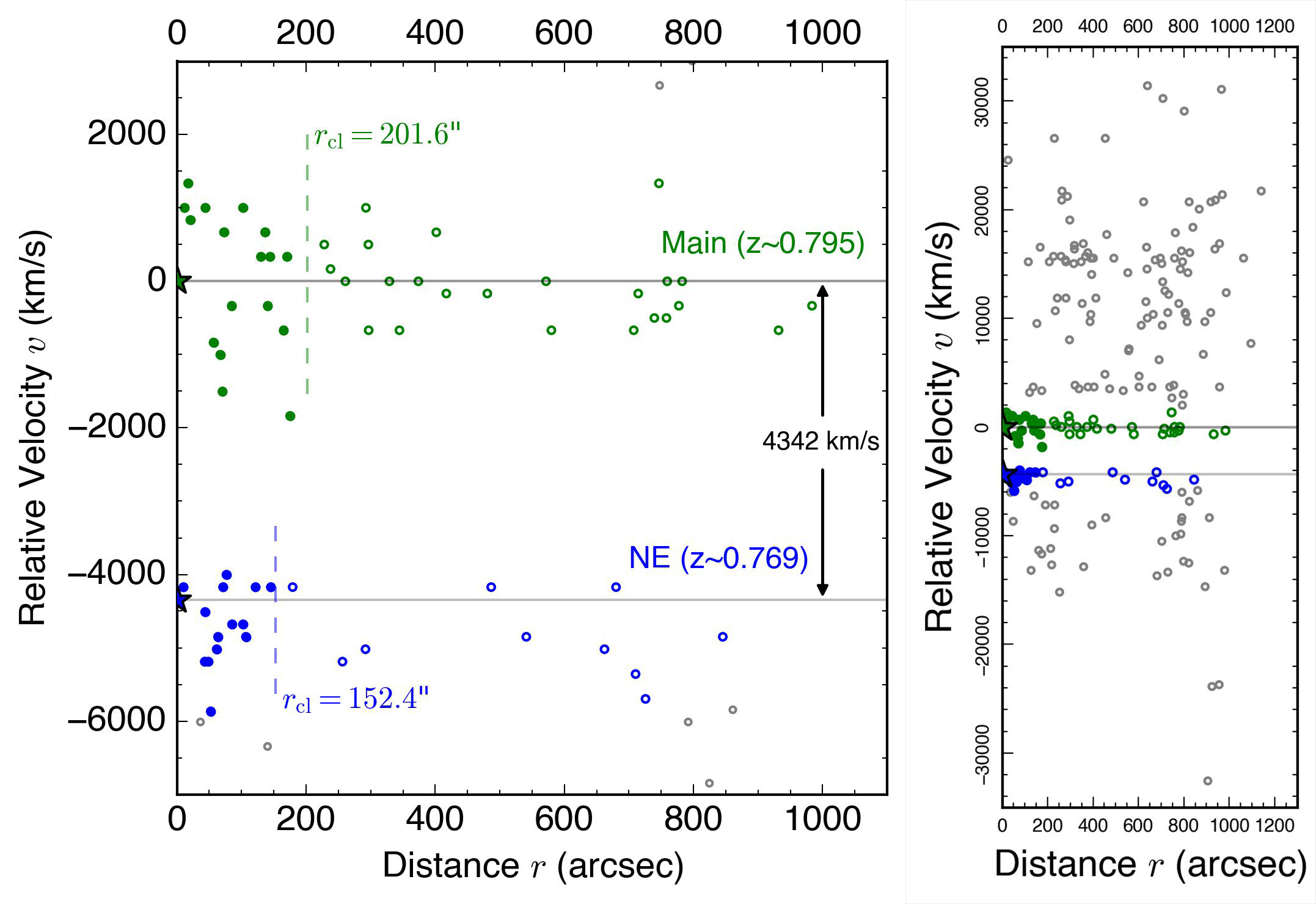
Figure 4: Plots of projected distance to cluster centre $r$ vs light-of-sight velocity $v$ for main and NE clusters. Green/Blue filled and open circles represent Main/NE cluster members inside and outside $r_{\mathrm{cl}}$ respectively. The grey open circles are non-cluster members. Left: Galaxies near $0.76\lesssim z_{\mathrm{spec}}\lesssim 0.81$ and right: $0.6\leq z_{\mathrm{spec}}\leq 1.0$.

3.2.3 Velocity Dispersion

Figure 4 plots the line-of-sight velocity distribution of galaxies, $v$, versus the projected distance from the cluster center, $r$. In this $r$-$v$ plot, the main cluster shows an expected trumpet shape with the velocity dispersion increasing toward the cluster center. For the NE cluster, the trumpet shape is not easy to identify, and many galaxies at larger $r$ show larger relative velocity offsets, making the cluster-member identification by the shifting gapper method critical.

The velocity dispersion of the NE and the main cluster members enclosed by $r_{\mathrm{cl}}$ are $\sigma_{\mathrm{NE}}=520\pm 90$ km s^-1and $\sigma_{\mathrm{main}}=930\pm 120$ km s^-1respectively, where the uncertainties of dispersion are derived from the Bootstrap resampling method. These velocity dispersions evaluated inside virialized cores provide key inputs for estimating the virial masses. Moreover, the velocity dispersions of member galaxies within $r_{200}$ are $\sigma_{\mathrm{200,NE}}=520\pm 100$  km s^-1 and $\sigma_{\mathrm{200,main}}=850\pm 110$  km s^-1from slightly smaller sample sizes (1 galaxy difference for NE and 2 for the main).

3.3 Color-Magnitude Diagram

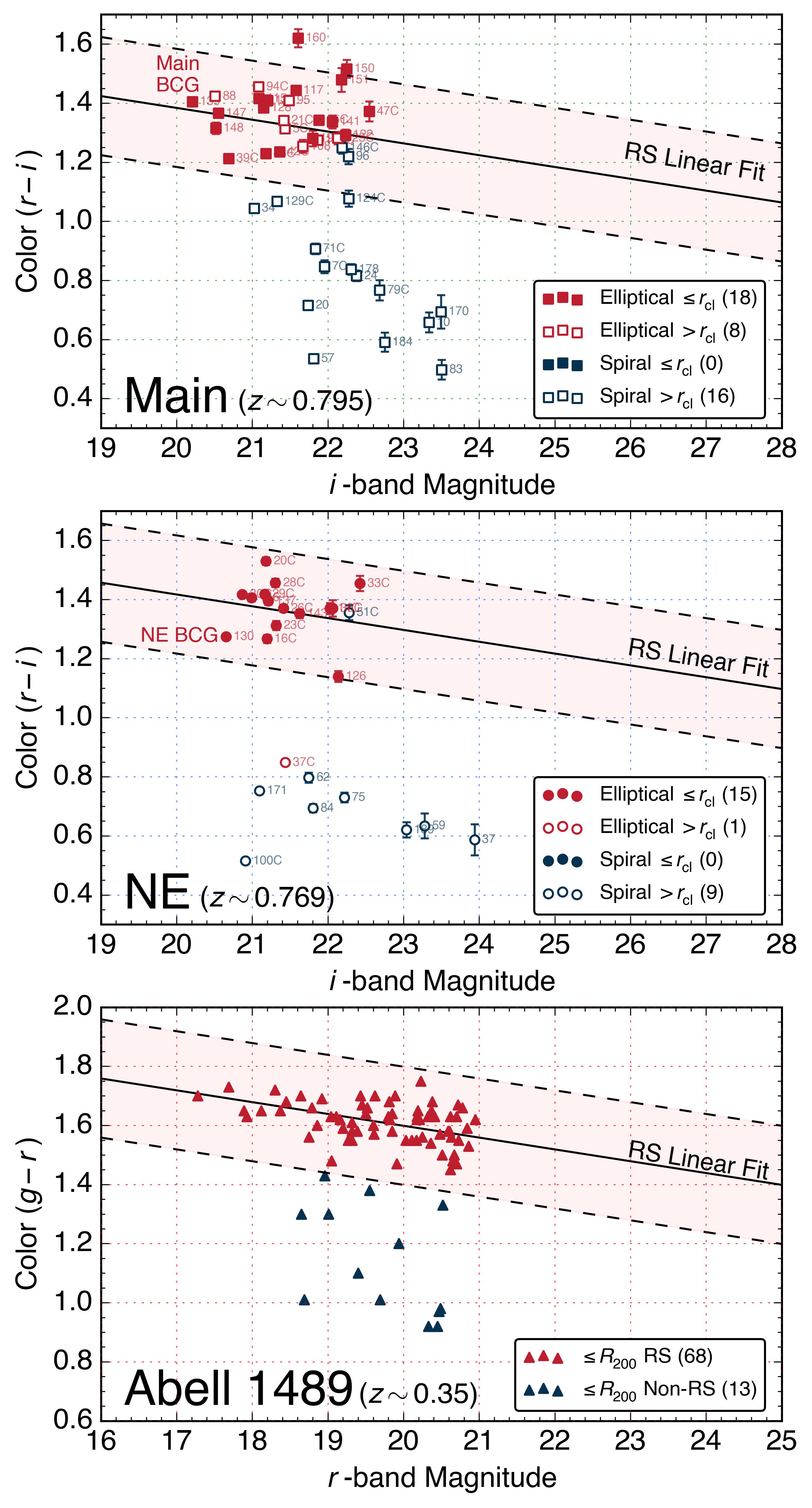
Figure 5: Top and Middle — Color-magnitude diagrams for the main and NE cluster-member galaxies with the HSC photometry. The red/blue color indicates the “elliptical”/“spiral” galaxies defined by the optical spectral features (see Section 3.3). The linear fit to the elliptical galaxies within $r_{\mathrm{cl}}$ (the solid lines) have the same fixed slope of $-0.04$. The dashed lines denote a range of $\Delta(r-i)=\pm 0.2$ from the fits, enclosing the red-sequence (RS) galaxies. Bottom — Color-magnitude Diagram for Abell 1489 cluster-member galaxies within $R_{200}$ as identified by Rines et al. (2022).

With the help of the HSC photometric catalog, we use confirmed cluster members to map out the color-magnitude diagrams. The HSC photometric catalog (Aihara et al., 2018) provides the galaxy’s broad-band magnitudes in the $r$ band ($\lambda_{\mathrm{eff}}$ $\sim$ 6175 Å, $\mathrm{FWHM}$ $=$ 1503 Å) and $i$ band ($\lambda_{\mathrm{eff}}$ $\sim$ 7711 Å, $\mathrm{FWHM}$ $=$ 1574 Å), which measure the Balmer/4000 Å breaks of $z\sim 0.8$ galaxies. In our color-magnitude analysis, the galaxies are matched with the HSC photometry data. Huang et al. (2018) give the typical precision of the HSC photometry as $\sim 0.023$ mag at $r=20$ mag, $\sim 0.036$ mag at $r=24$ mag, $\sim 0.015$ mag at $i=20$ mag, and $\sim 0.030$ mag at $i=24$ mag. With this photometric precision and the standard deviation of $\sim 0.004$ with the linear fit, the intercept uncertainty of the $(r-i)$ color is derived to be $0.03$.

We calculate the slope and intercept of the cluster RS as follows: First, we use spectral information to classify galaxy types: “elliptical” galaxies as those with strong Ca H&K and G-band absorption lines and “spiral” galaxies as those with emission lines (e.g. [O II] ${\lambda}$${\lambda}$3727, [O III], H$\gamma$). Second, we iterate to refine the membership of RS galaxies by (1) selecting the “elliptical” galaxies among galaxy cluster members within $r_{\mathrm{cl}}$, (2) fitting them with the provided slope of $-0.04$ (plotted with solid lines), and (3) filtering out those that have more than 0.2 color difference (indicated with dashed lines). Typically, the RS membership achieves stability after the second iteration.

In the main and NE cluster plots (Figure 5), their BCGs sit at the upper-left of the RS, confirming that BCGs are the brightest RS galaxies. The “elliptical” galaxies are located along the fitted RS line. The “spiral” galaxies look scattered downward from the RS line. The main cluster RS fit shows a $\Delta_{(r-i)}=0.11\pm 0.02$ mag scatter and an intercept $(r-i)=1.47\pm 0.03$ at $i=19$ mag. The scatter uncertainties are derived by the Bootstrap resampling (see Section 3.2.3). For the NE cluster, this gives a $\Delta_{(r-i)}=0.09\pm 0.02$ mag and an intercept of $(r-i)=1.46\pm 0.03$ as $i=19$ mag.

4 Discussion

4.1 No Association Between the Two Clusters

There is no significant overdensity of galaxies in the redshift/velocity space connecting the main and NE galaxy clusters at $0.77\lesssim z\lesssim 0.80$ in Figure 3 and  4. We note, however, that a merging cluster system may have high relative velocities resulting in a large separation in redshift/velocity space, even if they are physically close to each other. To determine whether or not the two galaxy clusters are physically associated, we can use the velocity difference ($4300$ km s^-1, see Figure 4) and compare it with the possible maximum velocity offset of merging systems from simulations.

Lee & Komatsu (2010) used $N$-body simulations of high-velocity merging clusters with the physical parameters similar to the galaxy cluster 1E0657-56 (i.e. “the Bullet Cluster”) to assess the likelihood of a satellite galaxy cluster merging with the main galaxy cluster. They showed that relative velocities of up to $\sim$ 2000–3000 km s^-1, measured at $(2-3)r_{200}$, could be produced by a merging event, but that a relative velocity of $>3000$ km s^-1 is rare for a merging system with a probability of only $3.6\times 10^{-9}$. Since the velocity offset between the main and NE clusters is $\sim 4300$ km s^-1, we conclude that the main and NE clusters are not physically associated with each other, and that their proximity is simply due to a projection along the line of sight.

Table 3: The Main and NE Cluster Dynamical Masses

	Virial mass ($<r_{\mathrm{cl}}$ $=1.2\times r_{200}$)						Scaling-relation mass ($<r_{200}$)				X-ray (T20)
	$N_{\mathrm{mem}}$	$R_{\mathrm{cl}}$	$R_{\mathrm{PV}}$	$\sigma_{\mathrm{P}}$	$M_{\mathrm{V}}$		$N_{\mathrm{mem}}$	$R_{200}$	$\sigma_{200}$	$M_{\mathrm{200}}$	$M_{\mathrm{200}}$
		(Mpc)	(Mpc)	( km s-1)	$(10^{14}$ M${}_{\sun})$			(Mpc)	( km s-1)	$(10^{14}$ M${}_{\sun})$	$(10^{14}$ M${}_{\sun})$
Main	18	1.5	1.2	$930\pm 120$	$8.6\pm 1.5$		16	1.3	$850\pm 110$	$3.8\pm 1.4$	$5.6^{+1.3}_{-0.8}$
NE	15	1.1	1.0	$520\pm~{}~{}90$	$3.3\pm 0.1$		14	0.9	$520\pm 100$	$1.0\pm 0.5$	$2.2^{+0.5}_{-0.3}$

4.2 Cluster Dynamical Masses

4.2.1 Virial Masses

We derived the virial masses for the two clusters by using the member galaxies within $r_{\mathrm{cl}}$ ($=1.2$ $r_{200}$). Below we follow the notation of Girardi et al. (1998). With the line-of-sight velocity of each galaxy, $V_{i}$, and the projected distance between the members $i$ and $j$ in the cluster, $R_{ij}$, the cluster virial mass can be expressed as,

$$M_{\mathrm{V}}=\frac{3\pi}{2}\frac{\sigma_{\mathrm{P}}^{2}R_{\mathrm{PV}}}{G},$$ (1)

where $G$ is the gravitational constant, $\sigma_{\mathrm{P}}$ is the projected velocity dispersion, and $R_{\mathrm{PV}}$ is the projected virial radius, which are calculated as

$$\sigma_{\mathrm{P}}=\sqrt{\frac{\textstyle\sum_{i}V_{i}^{2}}{N-1}},\;R_{\mathrm{PV}}=\frac{N(N-1)}{\textstyle\sum_{i>j}R_{ij}^{-1}},$$ (2)

where $N$ is the total number of galaxies in the cluster.

By following Girardi’s method, we derive the virial masses of the NE and main cluster as listed in Table 3. Since the observed member galaxies might not represent the entire population of the cluster system, Girardi et al. (1998) warn that the calculated mass overestimates the true mass with a median systematic offset of 19 to 39% because of different types of velocity anisotropy assumed for clusters (the so-called ”surface term”). Here, we assume a systematic offset of 30% and list the corrected masses $M_{\mathrm{V}}$ in Table 3.

4.2.2 Masses from the $\sigma_{200}$–M₂₀₀ Scaling Relation

$N$-body dark matter particle simulations suggest that there exists a scaling relation between the velocity dispersion of galaxies and cluster mass within $r_{200}$ (Evrard et al., 2008). We adopt the following scaling relation presented in Sifón et al. (2013, 2016):

$$\sigma_{200}=A_{\mathrm{1D}}\left(\frac{hE(z)M_{200}}{10^{15}\,\mathrm{M_{\sun}}}\right)^{\alpha}.$$ (3)

Here, $\sigma_{200}$ is the line-of-sight projected velocity dispersion of galaxies within $r_{200}$, and $M_{200}$ is the cluster mass within $r_{200}$. $\alpha$ was assumed to be $0.364\pm 0.002$. $A_{\mathrm{1D}}$ and $E(z)$ are expressed as follows: $A_{\mathrm{1D}}=1177\pm 4.2$ km s^-1, and $E(z)=\left(\Omega_{\Lambda}+(1+z)^{3}\Omega_{\mathrm{m}}\right)^{1/2}$. Table 3 lists the cluster masses derived from this method.

4.2.3 Comparison of Various Cluster-Mass Estimates

There is a systematic offset between the cluster dynamical masses derived with the virial theorem (Equation 1) and that with the $\sigma_{200}$–$M_{200}$ scaling relation (Equation 3). For example, if we assume a line-of-sight velocity dispersion of $\sigma_{\rm P}$ $=$ 1000 km s^-1 and a virial radius of $R_{\rm PV}$ $=$ 1 Mpc, the resultant viral mass $M_{\rm V}$ is $\approx$ $10^{15}$  M_☉, and with a 30% surface-term correction, $\approx$ $7\times 10^{14}$  M_☉. On the other hand, if we assume $R_{200}$ $\approx$ $R_{\rm PV}$ $=$ 1 Mpc and $\sigma_{200}$ $=$ $\sigma_{\rm P}$ $=$ 1000 km s^-1, the resultant $M_{200}$ is $4\times 10^{14}$  M_☉ at $z=0.8$, which is $\approx$ 60% of $M_{\rm V}$. As Table 3 shows, the observables themselves are similar ($R_{\rm PV}$ $\approx$ $R_{200}$ and $\sigma_{\rm P}$ $\approx$ $\sigma_{200}$), so the factor of a few difference between $M_{\rm V}$ and $M_{200}$ mainly comes from this systematic offset between the two methods.

Based on the XMM-Newton observations of this field, T20 reported X-ray-derived cluster masses of $5.6\times 10^{14}$ M_☉ for the EoH main cluster and $2.2\times 10^{14}$ M_☉ for the NE cluster, respectively. These X-ray-derived masses are between $M_{\rm V}$ and $M_{200}$. In the case of the main cluster, the X-ray mass is closer to $M_{200}$ while in the case of NE, it is in the middle of the two dynamical-mass estimates. Assuming that the X-ray-derived masses are closer to the true values, this indicates that both types of dynamical-mass estimates are equally good for the purpose of making a rough estimate (i.e., within a factor of $\sim$ 2 from the X-ray-derived masses) with a limited sampling of cluster members. $M_{\rm V}$ and $M_{200}$ are seen to result in an overestimate/underestimate, but the sample of two clusters here is simply too small to draw any general conclusion. The overall agreement of the dynamical and X-ray cluster masses also suggests that the cores of these two $z\sim 0.8$ clusters are already dynamically relaxed (i.e., virialized).

4.3 The NW Cluster Candidate

As described in Section 2.2, the slit mask in Run #2 was designed to cover the CAMIRA cluster candidate with a photometric redshift of $z_{\mathrm{CAMIRA}}=0.896$ located at the north-west of EoH (Figure 6, the blue squares in the top panel). Figure 3 also shows a redshift peak at $z\sim 0.89$, which matches the redshift of this cluster candidate.

Three of the CAMIRA-identified cluster members are found to have spectroscopic redshifts of 0.886, 0.893, and 0.896 (Figure 6, the top panel), hinting the existence of a cluster. However, three other cluster member candidates have spectroscopic redshifts outside the range of this putative cluster (which we define as $z$ $\approx$ 0.88–0.90). Although this is not surprising given the uncertainties of the photometric redshifts ($\sim$ 0.05 by Tanaka et al. 2018), it also prevents us from drawing a definitive conclusion about the reality of this CAMIRA-identified cluster. The Ca H&K lines at $z\sim 0.9$ are difficult to detect due to the B-band atmosphere absorption, which makes the redshift measurements difficult and only yields 6 galaxies with secure redshifts out of 13 galaxy candidates observed in the two observing runs.

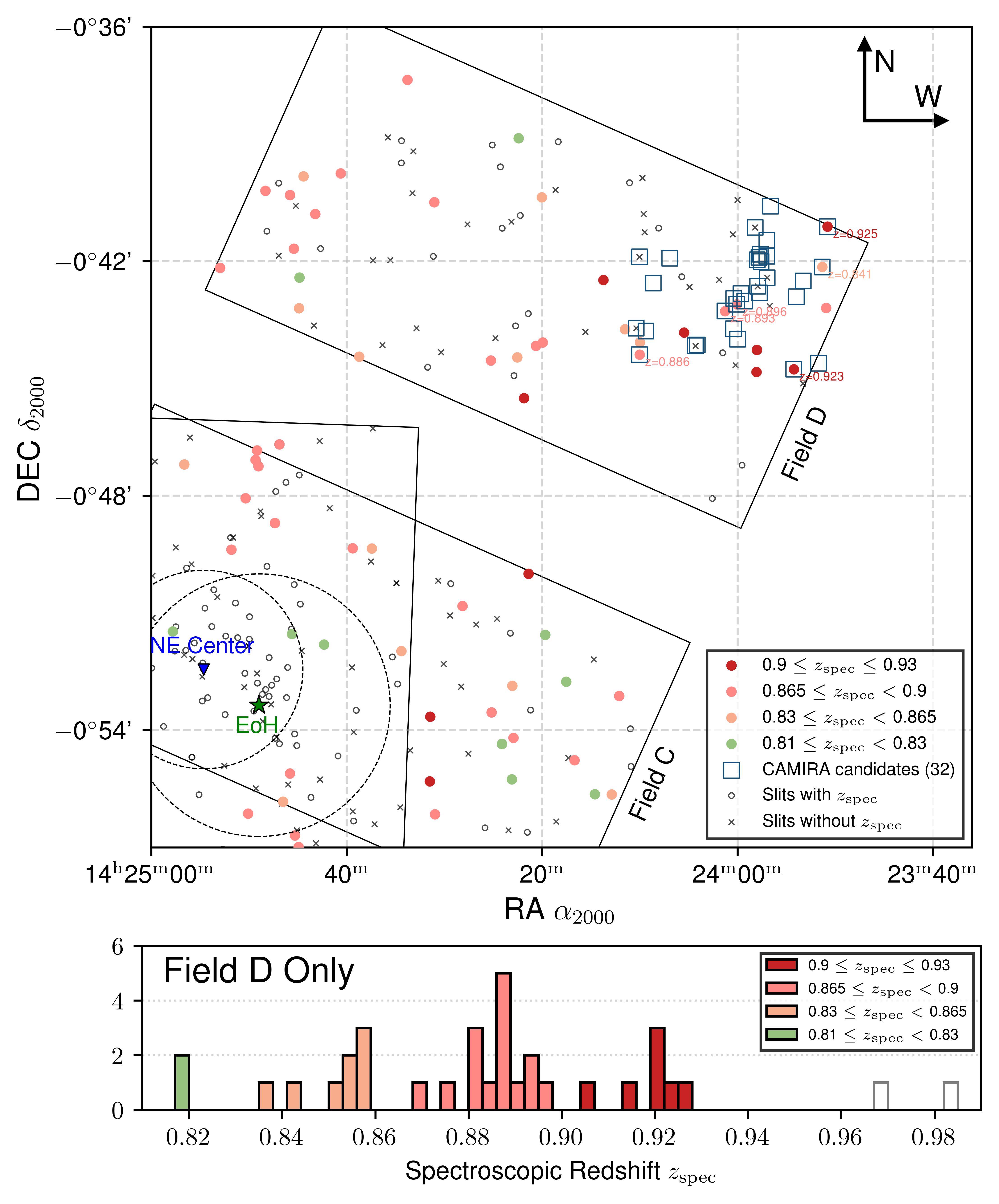
Figure 6: CAMIRA $z=0.896$ NW cluster candidate. Top — The sky positions of the Binospec slits are color-coded with redshifts. The locations of the CAMIRA-identified cluster-member galaxies are marked with the orange circles. Bottom — The redshift distribution is shown for galaxies in Field D only.

Figure 6 shows that $z\sim 0.9$ galaxies in Field D can be grouped into three redshift ranges: $0.830\leq z<0.865$, $0.865\leq z<0.900$, and $0.900\leq z<0.930$. However, none of these groupings exhibits any clear spatial clustering. In particular, galaxies in the redshift range of the NW cluster ($z$ $\approx$ 0.88–0.90) are distributed over Field D and even over Fields B and C, possibly suggesting a sheet-like structure (Figure 1 and 3).

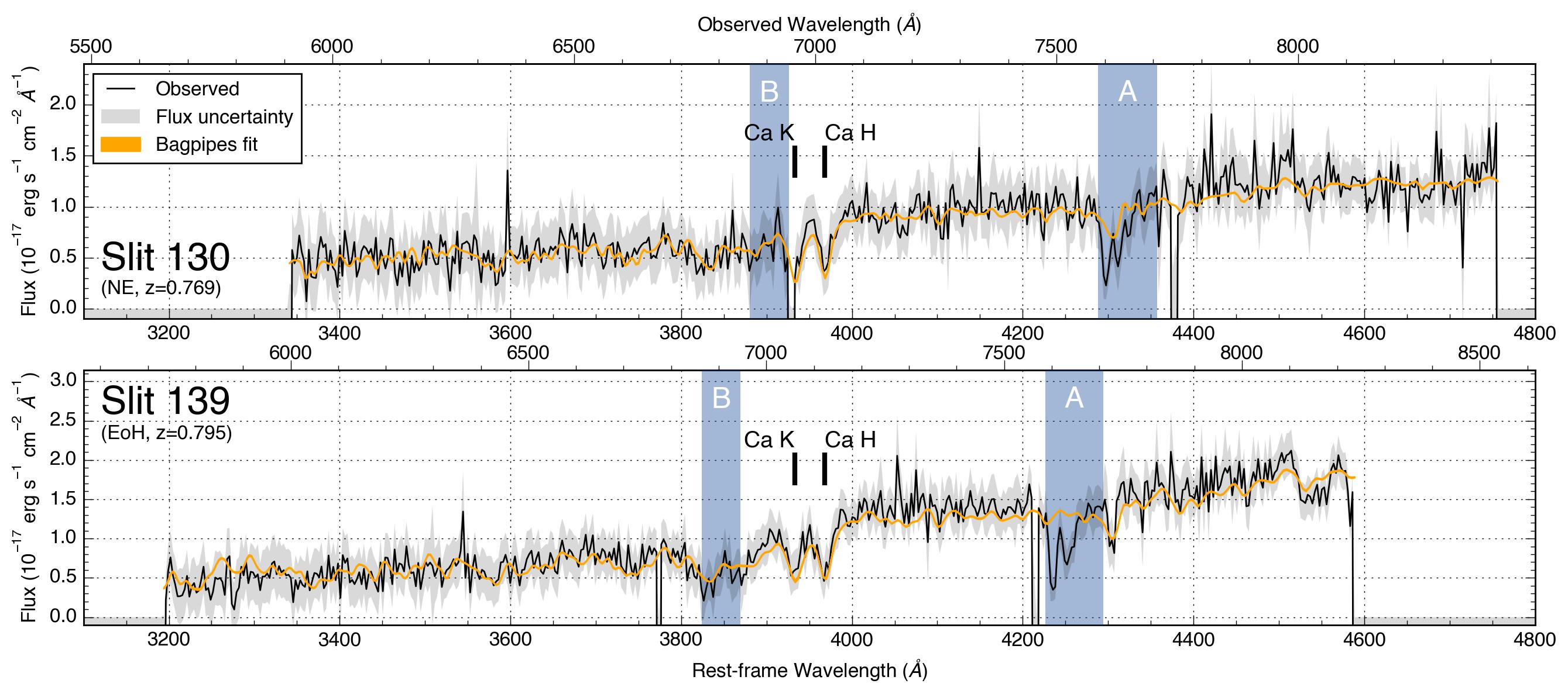
Figure 7: Bagpipes model fits to the spectra of the BCGs in the NE (Upper panel) and main (Middle panel) clusters. The orange model fits are generated by the Bagpipes posterior distribution with 1$\sigma$ error. The vertical blue bands at $\lambda\sim 7586-7708$ Å  and $\lambda\sim 6864-6945$ Å  are the A-band and B-band of the atmosphere absorption. The Ca H&K ${\lambda}{\lambda}3933,3968$ absorption lines are also indicated. The best-fit model spectra for the two BCGs are compared in the bottom panel. The best-fit spectrum of the main-cluster BCG has been re-scaled by 0.8 to match the continuum level shortward of the Ca K line.

4.4 Spectral Analysis of the two BCGs

Because of their brightnesses, the BCGs of the main cluster (EoH; Slit #139) and the NE cluster (Slit #130) produced high signal-to-noise Binospec spectra. We therefore performed spectral model fitting for them by using the program Bayesian Analysis of Galaxies for Physical Inference and Parameter EStimation (Bagpipes; Carnall et al., 2018). More specifically, we used the exponentially-declining star-formation history (SFH) with the following priors: the mass-weighted age $a/\mathrm{Gyr}\in(0.1,t_{\mathrm{universe}}(z_{\mathrm{obs}}))$, the exponential-decay parameter $\tau/\mathrm{Gyr}\in(0.3,10.0)$, the formed stellar mass $M_{\mathrm{formed}}/\mathrm{M}_{\sun}\in(10^{1},10^{15})$, the metalicity $Z/\mathrm{Z}_{\sun}\in(0.1,10.0)$, the absolute attenuation in V-band magnitudes $A_{\mathrm{V}}/\mathrm{mag}\in(0,2)$, and the velocity dispersion of the stellar component in the galaxy $\sigma_{\mathrm{*,vel}}/\mathrm{km}~{}\mathrm{s}^{-1}\in(10,1000)$. From derived quantities above after the fitting, Bagpipes will calculate the additional results, such as the current stellar mass $M_{\mathrm{*}}$.

Table 4: BCG Physical Properties from the Bagpipes Spectral-Model Fitting.

	Bagpipes							HSC/Mizuki
	Age $a/\mathrm{Gyr}$	$\tau/\mathrm{Gyr}$	$\log{\left(M_{\mathrm{formed}}/\mathrm{M}_{\sun}\right)}$	$\log{\left(Z/\mathrm{Z}_{\sun}\right)}$	$A_{\mathrm{V}}/\mathrm{mag}$	$\sigma_{\mathrm{*,vel}}/$ km s-1	$\log{\left(M_{*}/\mathrm{M}_{\sun}\right)}$	$\log{\left(M_{\mathrm{*,Mizuki}}/\mathrm{M}_{\sun}\right)}$
EoH	$3.6^{+0.4}_{-0.4}$	$0.6^{+0.1}_{-0.1}$	$11.98^{+0.04}_{-0.04}$	$0.8^{+0.1}_{-0.1}$	$0.08^{+0.07}_{-0.05}$	$340^{+20}_{-20}$	$11.61^{+0.04}_{-0.05}$	$11.53^{+0.04}_{-0.05}$ ($z_{\rm mizuki}$ $=$ 0.73)
NE	$6.0^{+0.6}_{-0.8}$	$0.5^{+0.2}_{-0.1}$	$11.62^{+0.04}_{-0.04}$	$0.4^{+0.1}_{-0.1}$	$0.07^{+0.09}_{-0.05}$	$310^{+60}_{-60}$	$11.30^{+0.01}_{-0.02}$	$11.29^{+0.04}_{-0.12}$ ($z_{\rm mizuki}$ $=$ 0.75)

Figure 7 compares the observed spectra of the two BCGs with the best-fit spectral models from Bagpipes. The model fits are seen to match the observed spectra quite well, reproducing the overall continuum shapes as well as those of the Ca H&K absorption lines. Table 4 lists the resultant best-fit parameters. The stellar velocity dispersion of the EoH BCG is measured to be $\sigma_{\mathrm{*,EoH}}=340^{+20}_{-20}$ km s^-1. Note that the error bars listed in the table only reflect the statistical uncertainties associated with the Bagpies fitting. For example, the uncertainties associated with the stellar mass $M_{\mathrm{*}}$ are $<$ 0.1 dex, consistent with those of other studies using Bagpipes ($\sim 0.06$ dex by Man et al., 2021), but the choice of the initial mass function alone could introduce a systematic uncertainty of $\sim 0.3$ dex (e.g., Mobasher et al., 2015; Carnall et al., 2019).

As expected, these two BCGs are old (age $=$ 3.6–6.0 Gyr) and massive ($M_{\mathrm{*}}$ $=$ 4.2–9.5 $\times$ $10^{11}$  M_☉). These spectroscopically derived stellar masses agree well with the photometrically derived ones from the HSC/Mizuki catalog as listed in Table 4 (Tanaka, 2015; Tanaka et al., 2018). Note, however, that these Mizuki stellar masses were derived with the Mizuki photometric redshifts for the BCGs, which are slightly different from our spectroscopic ones. The formation redshifts ($z_{\rm form}$) calculated from the Bagpipes-derived ages are $z\sim 2$ for the main-cluster BCG and $z\sim 7$ for the NE-cluster BCG, which are consistent with the range of $z_{\rm form}$ derived for quiescent galaxies in the SPT clusters in the same redshift range (Khullar et al., 2022).

Figure 7 overplots the two best-fit model spectra after scaling, showing that these two BCGs have very similar spectra. This reflects the fact that galaxy spectra do not change substantially at such old ages. Note that the 4000 Å break amplitude ($D_{4000}$) is larger for the EoH BCG although its derived stellar age is younger. This is likely due to the effect of this BCG having a larger metallicity (Table 4), reflecting the well-known age-metallicity degeneracy with old stellar populations (e.g., Worthey, 1994).

4.5 Red-Sequence Scatter

High-redshift clusters are expected to show an increased scatter with its RS because member galaxies are younger and exhibit a larger color variation. Observationally, however, it is not clear if this is really the case with $z\sim 1$ clusters. For example, some previous studies seem to indicate that the RS is already well-established in $z\sim 1$ galaxies, showing an RS color scatter that is as tight as those observed for lower-redshift clusters (e.g., Menci et al., 2008; Nishizawa et al., 2018).

In the bottom panel of Figure 5, we plot the color-magnitude diagram for the $z=0.351$ cluster Abell 1489 in comparison with those of the two $z\sim 0.8$ clusters presented in Section 3.3. Starting with the spectroscopically-confirmed cluster members within $R_{200}$ reported by Rines et al. (2022) and using the photometric magnitudes from the Dark Energy Camera Legacy Survey (Dey et al., 2019), we have identified 68 galaxies in the RS with a scatter of $\Delta_{(g-r)}=0.062\pm 0.005$ mag in the $(g-r)$ color (Figure 5, the bottom penel). This RS color scatter is significantly smaller (1.5–1.8 $\times$) than $0.11\pm 0.02$ with the main cluster and $0.09\pm 0.02$ with the NE cluster, suggesting the possibility that the RS scatter does increase with $z\sim 1$ clusters.

5 Conclusions

In this paper, we used MMT/Binospec to conduct a spectroscopic survey to study two $z\sim 0.8$ galaxy clusters in the “Eye of Horus” lens system field. Our findings are as follows:

1. We have spectroscopically confirmed the existence of two galaxy clusters in the EoH field, the main cluster at $z=0.795$ (42 $z_{\rm spec}$ members) and the NE cluster (25 $z_{\rm spec}$ members) at $0.769$, corresponding to the two X-ray sources detected by XMM-Newton. The two clusters have a small separation on the sky ($\sim$ 100″ $=$ 0.75 Mpc $<r_{200}$), but a velocity offset of $\sim$4300 km s^-1 suggests that this two-cluster system is likely a line-of-sight projection rather than a physically-related association (e.g., a cluster merger). This underscores the importance of conducting a spectroscopic follow-up for high-redshift cluster candidates because RS-based cluster selections are susceptible to such a projection effect in general.

2. The masses of the main and NE clusters are estimated dynamically to be 8.6 and 3.3 $\times$ $10^{14}$  M_☉ with the virial theorem and 3.8 and 1.0 $\times$ $10^{14}$  M_☉ with the $\sigma_{200}$ – $M_{\mathrm{200}}$ scaling relation. Broadly speaking, these dynamical masses agree with the X-ray-derived ones within a factor of two; However, the virial masses are systematically larger than the $\sigma_{200}$ – $M_{\mathrm{200}}$ scaling masses by a factor of a few.

3. The spectral analysis of the BCGs in the main and NE clusters shows that these galaxies are already old (Age $=$ 3.6–6.0 Gyr) and massive ($M_{\mathrm{*}}$ $=$ 4.2–9.5 $\times$ $10^{11}$  M_☉), similar to the BCGs in lower-redshift clusters.

4. The color-magnitude diagrams of the main and NE clusters show an RS scatter of $\sim$0.1 mag, which appears significantly larger (1.5–1.8 $\times$) than that of a $z=0.35$ cluster in comparison. A more extensive comparison of spectrscopically-confirmed members in low- and high-redshift clusters is needed to make a more robust assessment.

Appendix A Redshift Table

We provide the full redshift catalog including 371 sources in Table 5, which combines the 2019 and 2022 MMT/Binospec observations over the four fields shown in Figure 1: Slit #1–86 (Field A) and Slit #87–190 (Field B) in 2019; Slit #1C–96C (Field C) and Slit #97C–181C (Field D) in 2022. In the “Notes” column, the reasons are provided for those slits that did not produce secure redshifts.

Table 5: Redshift Table for the 2019 and 2022 MMT/Binospec Observations

Slit	Redshift	RA	DEC	Lines	Confidence	Notes
1	-	216.38562	-0.76420	-	1
2	0.813	216.38863	-0.76642	Ca H&K	3
3	-	216.44077	-0.76689	-	1	noise
4	0.858	216.43033	-0.77128	[O II] ${\lambda}$3727	3
5	0.864	216.33951	-0.77705	Ca H&K	3
6	0.759	216.39340	-0.77723	[O II] ${\lambda}$3727	3
7	0.745	216.43243	-0.77912	[O II] ${\lambda}$3727	3
8	-	216.39641	-0.78259	-	1	continue (no spectrum feature)
9	-	216.39623	-0.78598	-	1	faint continue (no spectrum feature)
10	0.795	216.39694	-0.78897	[O II] ${\lambda}$3727	3
11	-	216.39259	-0.79164	-	1	noise
12	-	216.39078	-0.79438	-	1	point source, [O II] ${\lambda}$3727-overlapped
13	0.811	216.39064	-0.79803	[O II] ${\lambda}$3727	3
14	0.858	216.38635	-0.80063	Ca H&K	3
15	1.070	216.41468	-0.80203	[O II] ${\lambda}$3727	3
16	0.832	216.37693	-0.80564	[O II] ${\lambda}$3727	3
17	0.818	216.39775	-0.80834	[O II] ${\lambda}$3727	3
18	0.863	216.40519	-0.81001	[O II] ${\lambda}$3727	3
19	0.817	216.39466	-0.81343	[O II] ${\lambda}$3727	3
20	0.803	216.39791	-0.81548	[O II] ${\lambda}$3727	3
21	-	216.39976	-0.81736	-	1	noise
22	-	216.40978	-0.82074	-	1	faint continue (no spectrum feature)
23	0.817	216.35927	-0.82625	Ca H&K	3
24	0.794	216.39286	-0.82796	[O II] ${\lambda}$3727	3
25	-	216.35929	-0.83292	-	3	M6 star - monitor atm
26	-	216.41304	-0.83380	-	1	point source, [O II] ${\lambda}$3727-overlapped
27	-	216.37556	-0.83763	-	1	noise, as faint as 048
28	-	216.36190	-0.84013	-	1	[O II] ${\lambda}$3727-overlapped
29	0.743	216.41831	-0.84203	Ca H&K	3
30	0.796	216.39969	-0.84611	[O II] ${\lambda}$3727	1
31	0.823	216.36726	-0.85097	[O II] ${\lambda}$3727	3
32	0.976	216.39745	-0.85292	[O II] ${\lambda}$3727	3
33	-	216.38826	-0.85619	-	1	[O II] ${\lambda}$3727-overlapped
34	0.793	216.41769	-0.85725	[O II] ${\lambda}$3727	3
35	-	216.41113	-0.86031	-	1	noise
36	0.855	216.38017	-0.86529	[O II] ${\lambda}$3727	3
37	0.765	216.41153	-0.86742	[O II] ${\lambda}$3727	3
38	0.942	216.38731	-0.87103	[O II] ${\lambda}$3727	1
39	0.870	216.40269	-0.87345	[O II] ${\lambda}$3727	3	two galaxies, redshift for lower one
40	0.848	216.35439	-0.87967	Ca H&K	1	first type 0.858, then adjust
41	-	216.42898	-0.88117	-	1	noise
42	-	216.42185	-0.88452	-	1	noise
43	-	216.43421	-0.88606	-	1	noise
44	0.721	216.42609	-0.88873	[O II] ${\lambda}$3727	3
45	-	216.36506	-0.89389	-	1	noise
46	-	216.42594	-0.89454	-	1	noise
47	-	216.40032	-0.89771	-	1	continue (no spectrum feature)
48	-	216.40650	-0.90146	-	1	noise, as faint as 027
49	1.028	216.40205	-0.90398	[O II] ${\lambda}$3727	3
50	0.894	216.37999	-0.90689	[O II] ${\lambda}$3727	3
51	1.030	216.37827	-0.90895	[O II] ${\lambda}$3727	1
52	-	216.40155	-0.91211	-	1	noise
53	-	216.40548	-0.91505	-	1	faint continue (no spectrum feature)
54	-	216.43441	-0.91627	-	1	faint continue (no spectrum feature)
55	0.754	216.43136	-0.91855	[O II] ${\lambda}$3727	3
56	-	216.40117	-0.92251	-	1	noise
57	0.792	216.41158	-0.92571	[O II] ${\lambda}$3727	3
58	-	216.33630	-0.93211	-	1	noise
59	0.761	216.42056	-0.93288	[O II] ${\lambda}$3727	3
60	0.919	216.42847	-0.93454	[O II] ${\lambda}$3727	3
61	0.710	216.39817	-0.93757	Ca H&K	1
62	0.766	216.36198	-0.94169	[O II] ${\lambda}$3727	3
63	0.851	216.39249	-0.94331	[O II] ${\lambda}$3727	3
64	-	216.37143	-0.94660	-	1	faint continue (no spectrum feature)
65	-	216.43833	-0.94805	-	1	faint continue (no spectrum feature)
66	0.868	216.39797	-0.95193	[O II] ${\lambda}$3727	3
67	-	216.37452	-0.95666	-	1	noise
68	-	216.41021	-0.95747	-	1	faint continue (no spectrum feature)
69	0.713	216.37940	-0.96138	[O II] ${\lambda}$3727	3	two galaxies, redshift for middle
70	-	216.40184	-0.96304	-	1	faint continue (no spectrum feature)
71	-	216.40042	-0.96664	-	1	faint continue (no spectrum feature)
72	0.902	216.40058	-0.96880	[O II] ${\lambda}$3727	3
73	-	216.42254	-0.97060	-	1	$z=$0.894 if [O II] ${\lambda}$3727 overlapped
74	-	216.37381	-0.97441	-	1	$z=$0.986 if CaK,CaH overlapped
75	0.766	216.43996	-0.97465	[O II] ${\lambda}$3727	3
76	-	216.39145	-0.97886	-	1	$z=$0.904 if [O II] ${\lambda}$3727 overlapped
77	-	216.43429	-0.98117	-	1	$z=$0.690 if [O II] ${\lambda}$3727 overlapped
78	0.981	216.45543	-0.98347	[O II] ${\lambda}$3727	3
79	0.835	216.43017	-0.98669	[O II] ${\lambda}$3727	3
80	0.745	216.39819	-0.99283	[O II] ${\lambda}$3727	3
81	-	216.40618	-0.99636	-	1	noise
82	-	216.39960	-0.99873	-	1	$z=$0.389 if Mg-Na
83	0.795	216.38280	-1.00149	[O II] ${\lambda}$3727	3
84	0.763	216.37536	-1.00503	[O II] ${\lambda}$3727	3
85	-	216.38575	-1.00944	-	1	cannot tell
86	0.736	216.38540	-1.01161	[O II] ${\lambda}$3727	3
87	-	216.15565	-0.77128	-	1	cannot tell
88	0.794	216.26665	-0.77135	Ca H&K	3
89	-	216.17817	-0.77663	-	1	noise
90	0.888	216.19541	-0.77813	Ca H&K,G	3
91	0.888	216.20494	-0.78072	[O II] ${\lambda}$3727	3
92	0.891	216.20558	-0.78467	Ca H&K	3
93	0.889	216.20434	-0.78738	[O II] ${\lambda}$3727	3
94	0.718	216.18694	-0.79120	[O II] ${\lambda}$3727	3
95	0.791	216.19260	-0.79432	Ca H&K	3
96	0.795	216.19694	-0.79822	[O II] ${\lambda}$3727	3
97	0.893	216.20984	-0.80107	[O II] ${\lambda}$3727	3
98	-	216.17398	-0.80534	-	1	noise
99	-	216.20353	-0.80667	-	1	noise
100	0.823	216.20321	-0.80868	Ca H&K	1	suspicious spot above continuum
101	0.866	216.19738	-0.81166	[O II] ${\lambda}$3727	3
102	-	216.26411	-0.81330	-	1	noise
103	-	216.21523	-0.81777	-	1	noise
104	0.886	216.16421	-0.82239	[O II] ${\lambda}$3727	3
105	0.866	216.21594	-0.82295	[O II] ${\lambda}$3727	3
106	-	216.15638	-0.82810	-	1	$z=$0.885?, cannot tell
107	0.728	216.20069	-0.83015	[O II] ${\lambda}$3727	3
108	0.796	216.23497	-0.83090	Ca H&K	3
109	-	216.14556	-0.83733	-	1	noise
110	1.159	216.18907	-0.83791	[O II] ${\lambda}$3727	3
111	0.752	216.22337	-0.84014	[O II] ${\lambda}$3727	3
112	0.922	216.22195	-0.84322	Ca H&K,G	1
113	-	216.22195	-0.84322	-	1	faint continue (no spectrum feature)
114	0.727	216.21412	-0.84580	Ca H&K	3
115	0.797	216.22715	-0.84796	Ca H&K	3
116	0.796	216.22715	-0.84796	Ca H&K	3
117	0.799	216.20813	-0.85164	Ca H&K	3
118	-	216.24958	-0.85213	-	1	faint continue (no spectrum feature)
119	0.716	216.19024	-0.85687	Ca H&K	3
120	0.815	216.24089	-0.85787	Ca H&K	3
121	0.814	216.24089	-0.85787	Ca H&K	3
122	0.801	216.20820	-0.86123	Ca H&K	3
123	0.801	216.20820	-0.86123	Ca H&K	3
124	-	216.20860	-0.86411	-	1
125	0.757	216.23533	-0.86596	Ca H&K,G	3
126	0.767	216.19977	-0.86907	Ca H&K,G	3
127	0.767	216.19977	-0.86907	Ca H&K,G	3
128	0.799	216.19187	-0.87327	Ca H&K,G	3
129	0.799	216.19187	-0.87327	Ca H&K,G	3
130	0.769	216.22772	-0.87414	Ca H&K	3
131	0.743	216.19654	-0.87817	G	3
132	0.758	216.19654	-0.87817	-	1
133	0.759	216.19869	-0.88085	Ca H&K	3
134	0.942	216.20126	-0.88268	[O II] ${\lambda}$3727	2
135	0.803	216.20265	-0.88476	Ca H&K,G	3
136	0.802	216.20265	-0.88476	Ca H&K,G	3
137	0.768	216.22598	-0.88614	Ca H&K	3
138	0.768	216.22598	-0.88614	Ca H&K	3
139	0.795	216.20415	-0.88935	Ca H&K	3
140	0.795	216.20415	-0.88935	Ca H&K	3
141	0.801	216.20628	-0.89187	Ca H&K	3
142	0.801	216.20628	-0.89187	Ca H&K	3
143	0.771	216.21853	-0.89336	Ca H&K,G	3
144	-	216.20257	-0.89612	-	1	faint continue (no spectrum feature)
145	-	216.20257	-0.89612	-	1	two galaxies
146	0.766	216.24479	-0.89843	Ca H&K	3
147	0.790	216.19721	-0.90350	Ca H&K	3
148	0.789	216.19537	-0.90580	Ca H&K,G	3
149	-	216.27081	-0.90572	-	1	noise
150	0.797	216.17039	-0.91103	Ca H&K,G	3
151	0.797	216.23269	-0.91152	Ca H&K,G	3
152	-	216.23269	-0.91152	-	1	noise
153	-	216.21902	-0.91517	-	1	noise
154	0.886	216.19092	-0.91847	[O II] ${\lambda}$3727	3
155	-	216.17814	-0.92103	-	1	noise
156	-	216.17814	-0.92103	-	1	noise
157	-	216.19165	-0.92317	-	1	noise
158	-	216.19165	-0.92317	-	1	noise
159	-	216.20553	-0.92485	-	1	noise
160	0.791	216.22966	-0.92755	Ca H&K,G	3
161	0.791	216.22966	-0.92755	Ca H&K	3
162	-	216.19424	-0.93132	-	1	noise
163	-	216.16414	-0.93462	-	1	noise
164	0.894	216.20880	-0.93560	[O II] ${\lambda}$3727	3
165	-	216.15486	-0.94014	-	1	noise
166	-	216.18801	-0.94266	-	1	noise
167	0.886	216.18882	-0.94494	[O II] ${\lambda}$3727	3
168	0.752	216.17984	-0.94817	G	1
169	0.889	216.18723	-0.94986	Ca H&K,G	3
170	0.798	216.21948	-0.95084	[O II] ${\lambda}$3727	3
171	0.765	216.21633	-0.95445	[O II] ${\lambda}$3727	3
172	0.920	216.18011	-0.95817	-	2	several absorption lines with continue
173	0.889	216.19767	-0.96103	[O II] ${\lambda}$3727	3
174	-	216.17484	-0.96385	-	1	noise
175	0.887	216.22087	-0.96487	[O II] ${\lambda}$3727	3
176	0.909	216.23340	-0.96672	[O II] ${\lambda}$3727	3
177	-	216.23521	-0.96883	-	1	noise
178	0.791	216.21121	-0.97154	[O II] ${\lambda}$3727	3
179	0.885	216.22268	-0.97496	[O II] ${\lambda}$3727	3
180	-	216.21390	-0.97788	-	1	noise
181	0.816	216.19365	-0.98274	[O II] ${\lambda}$3727	3
182	-	216.19471	-0.98489	-	1	noise
183	0.863	216.20702	-0.98722	[O II] ${\lambda}$3727	3
184	0.795	216.18229	-0.99090	[O II] ${\lambda}$3727	3
185	-	216.24355	-0.99683	-	1	noise
186	-	216.23331	-0.99970	-	1	faint continue (no spectrum feature)
187	0.866	216.21658	-1.00330	[O II] ${\lambda}$3727	3
188	-	216.20184	-1.00635	-	1	faint continue (no spectrum feature)
189	0.770	216.22189	-1.00922	[O II] ${\lambda}$3727	3
190	-	216.18153	-1.01652	-	1	continue (no spectrum feature)
1C	-	216.26140	-0.79481	-	1	noise
2C	1.029	216.25806	-0.79324	[O II] ${\lambda}$3727	3
3C	0.818	216.29276	-0.87998	Ca H&K	3
4C	-	216.24861	-0.78536	-	1	faint continue (no spectrum feature)
5C	0.801	216.27079	-0.84277	Ca H&K	3
6C	-	216.26300	-0.82987	-	1	noise
7C	0.798	216.25903	-0.82793	[O II] ${\lambda}$3727	3
8C	-	216.23356	-0.77519	-	1	emission line $\sim 6400$ Å
9C	0.853	216.23602	-0.78668	[O II] ${\lambda}$3727	3
10C	0.704	216.25897	-0.84544	Ca H&K	3
11C	-	216.24960	-0.83405	-	1	noise
12C	0.752	216.26768	-0.87993	[O II] ${\lambda}$3727	2	CaHK behind B-Band
13C	-	216.23961	-0.82203	-	1	noise
14C	0.770	216.26605	-0.88703	Ca H&K	3
15C	0.739	216.26768	-0.89618	Ca H&K	2	CaHK behind B-Band
16C	0.770	216.25982	-0.88481	Ca H&K	3
17C	-	216.23293	-0.82923	-	1	faint continue (no spectrum feature)
18C	0.725	216.24985	-0.87355	[O II] ${\lambda}$3727	3
19C	0.784	216.23953	-0.85591	Ca H&K	3
20C	0.760	216.23997	-0.86629	Ca H&K	3
21C	0.795	216.21621	-0.81791	Ca H&K	3
22C	-	216.23613	-0.86787	-	1	no signal
23C	0.764	216.23169	-0.86283	Ca H&K	3	bad sky subtraction
24C	-	216.23255	-0.86959	-	1
25C	0.793	216.22423	-0.85582	Ca H&K	3	bad sky subtraction
26C	0.770	216.22806	-0.87133	Ca H&K,G	3
27C	-	216.22826	-0.87711	-	1	noise
28C	0.765	216.21826	-0.85989	Ca H&K,G	3	two continues, take lower one
29C	0.764	216.22830	-0.88758	Ca H&K,G	3	wonderful features
30C	0.770	216.21318	-0.86057	Ca H&K,G	3
31C	0.797	216.23269	-0.91152	Ca H&K	2	(=Slit #151/152)
32C	-	216.20860	-0.86412	-	1	(=Slit #124) CaHK behind A-Band
33C	0.766	216.21012	-0.87577	Ca H&K	3	faint continue (no spectrum feature)
34C	-	216.21044	-0.88164	-	1	noise
35C	-	216.20496	-0.87575	-	1	noise
36C	0.767	216.20475	-0.87996	Ca H&K	3	bad sky subtraction
37C	0.770	216.18647	-0.84626	Ca H&K,G	3
38C	0.814	216.19002	-0.85895	Ca H&K,G	3
39C	0.800	216.19978	-0.88561	Ca H&K,G	3
40C	-	216.19898	-0.88894	-	1	faint continue (no spectrum feature)
41C	-	216.18590	-0.86616	-	1	noise
42C	0.801	216.19233	-0.88613	Ca H&K,G	3
43C	-	216.19664	-0.90295	-	1	noise
44C	0.817	216.17641	-0.86347	Ca H&K,G	3
45C	0.843	216.15603	-0.82251	[O II] ${\lambda}$3727	3
46C	0.786	216.18890	-0.90164	Ca H&K,G	3
47C	0.793	216.18799	-0.90658	Ca H&K,G	3
48C	0.852	216.19391	-0.93053	Ca H&K	3
49C	-	216.16449	-0.87315	-	1	noise
50C	-	216.14556	-0.83733	-	1	(=Slit #109) noise
51C	0.764	216.18193	-0.92870	[O II] ${\lambda}$3727	3
52C	1.070	216.16261	-0.89155	[O II] ${\lambda}$3727	3
53C	-	216.16368	-0.90076	-	1	no signal
54C	0.719	216.14721	-0.86878	[O II] ${\lambda}$3727	3
55C	0.859	216.14340	-0.86622	[O II] ${\lambda}$3727	3
56C	-	216.12775	-0.83622	-	1	faint continue (no spectrum feature)
57C	0.570	216.14499	-0.88034	Ca H&K,G	3
58C	0.083	216.12232	-0.83752	M6	3	M6 star
59C	0.954	216.16373	-0.93877	[O II] ${\lambda}$3727	3
60C	-	216.12265	-0.85105	-	1	bad sky subtraction
61C	0.886	216.11735	-0.84704	[O II] ${\lambda}$3727	3
62C	-	216.12537	-0.87170	-	1	bad sky subtraction
63C	-	216.13969	-0.90858	-	1	faint continue (no spectrum feature)
64C	0.925	216.13108	-0.89423	[O II] ${\lambda}$3727	3
65C	-	216.11152	-0.85490	-	1	bad sky subtraction
66C	-	216.14387	-0.93289	-	1	faint continue (no spectrum feature)
67C	-	216.11791	-0.88143	-	1	faint continue (no spectrum feature)
68C	-	216.10263	-0.85251	-	1	no signal
69C	0.922	216.13127	-0.92183	[O II] ${\lambda}$3727	3
70C	0.901	216.08915	-0.83328	[O II] ${\lambda}$3727	3
71C	0.799	216.09688	-0.85866	[O II] ${\lambda}$3727	3
72C	0.895	216.12903	-0.93589	[O II] ${\lambda}$3727	3	bottom: blue galaxy at $z=$0.102
73C	-	216.11488	-0.90999	-	1	faint continue (no spectrum feature)
74C	0.896	216.10496	-0.89238	Ca H&K,G	3
75C	0.857	216.09606	-0.88104	[O II] ${\lambda}$3727	3
76C	0.824	216.08203	-0.85937	Ca H&K	3	faint with distinguishable feature
77C	0.817	216.10053	-0.90584	[O II] ${\lambda}$3727	3
78C	0.879	216.09559	-0.90328	[O II] ${\lambda}$3727	3
79C	0.794	216.08827	-0.89147	[O II] ${\lambda}$3727	3
80C	0.741	216.10771	-0.94168	Ca H&K	3
81C	0.817	216.09630	-0.92098	Ca H&K	3
82C	0.816	216.07308	-0.87937	Ca H&K	3
83C	-	216.09774	-0.94265	-	1	no signal
84C	-	216.06135	-0.86983	-	1	noise
85C	0.954	216.09830	-0.95793	[O II] ${\lambda}$3727	3
86C	0.745	216.08964	-0.94358	[O II] ${\lambda}$3727	3
87C	-	216.07222	-0.91188	-	1	noise
88C	0.888	216.06954	-0.91276	Ca H&K	3
89C	-	216.07734	-0.93897	-	1	faint continue (no spectrum feature)
90C	0.880	216.05048	-0.88543	[O II] ${\lambda}$3727	3
91C	1.097	216.07754	-0.95224	[O II] ${\lambda}$3727	3
92C	-	216.08556	-0.97561	-	1	faint continue (no spectrum feature)
93C	0.815	216.06094	-0.92736	[O II] ${\lambda}$3727	3
94C	0.795	216.04568	-0.89943	Ca H&K,G	3	wonderful features
95C	0.838	216.05368	-0.92740	[O II] ${\lambda}$3727	3
96C	0.134	216.04542	-0.91551	H $\alpha$ ${\lambda}$6563	3	green galaxy or quasar
97C	0.887	216.22066	-0.70284	[O II] ${\lambda}$3727	3
98C	0.892	216.20140	-0.66991	[O II] ${\lambda}$3727	3
99C	0.969	216.19570	-0.66670	[O II] ${\lambda}$3727	3
100C	0.770	216.20072	-0.68718	[O II] ${\lambda}$3727	3	wonderful features
101C	0.882	216.19088	-0.67172	[O II] ${\lambda}$3727	3
102C	0.853	216.18517	-0.66378	[O II] ${\lambda}$3727	3
103C	-	216.18842	-0.67635	-	1	noise
104C	-	216.19569	-0.69759	-	1	continue but no spectrum feature
105C	0.885	216.18930	-0.69458	[O II] ${\lambda}$3727	2	another emission at $7700$ Å
106C	0.888	216.18011	-0.67982	Ca H&K,G	3	faint with distinguishable feature
107C	0.891	216.16926	-0.66255	[O II] ${\lambda}$3727	3
108C	0.817	216.18688	-0.70697	[O II] ${\lambda}$3727	3
109C	0.791	216.17784	-0.69461	Ca H&K	3
110C	0.851	216.18703	-0.72003	[O II] ${\lambda}$3727	3
111C	0.869	216.14085	-0.62258	Ca H&K	3
112C	-	216.14917	-0.64708	-	1	noise
113C	-	216.18067	-0.72742	-	1	noise
114C	0.707	216.14331	-0.64860	[O II] ${\lambda}$3727	3
115C	0.760	216.14338	-0.65805	[O II] ${\lambda}$3727	3
116C	-	216.13829	-0.65307	-	1	continue but no spectrum feature
117C	-	216.15551	-0.69953	-	1	noise
118C	-	216.13871	-0.67097	-	1	continue but no spectrum feature
119C	-	216.14815	-0.69955	-	1	continue but no spectrum feature
120C	0.837	216.16138	-0.74069	[O II] ${\lambda}$3727	3
121C	0.880	216.12934	-0.67482	[O II] ${\lambda}$3727	3	wonderful features
122C	-	216.15143	-0.73580	-	1	faint continue (no spectrum feature)
123C	0.792	216.12973	-0.69792	Ca H&K	3
124C	0.791	216.10461	-0.65042	[O II] ${\lambda}$3727	3
125C	-	216.13700	-0.72860	-	1	too bright background
126C	-	216.11520	-0.68423	-	1	noise
127C	0.600	216.10112	-0.65974	[O II] ${\lambda}$3727,H $\gamma$,H $\beta$,[O III]	3
128C	0.817	216.09341	-0.64750	[O II] ${\lambda}$3727	3
129C	0.791	216.13217	-0.74523	[O II] ${\lambda}$3727	3
130C	-	216.12651	-0.73876	-	1	noise
131C	0.720	216.10037	-0.68593	[O II] ${\lambda}$3727	3
132C	-	216.09644	-0.68313	-	1	noise
133C	0.557	216.09266	-0.68048	[O II] ${\lambda}$3727	3
134C	0.716	216.07647	-0.64902	[O II] ${\lambda}$3727	3
135C	0.853	216.08352	-0.67267	[O II] ${\lambda}$3727	3
136C	-	216.07764	-0.66950	-	1	noise
137C	-	216.10327	-0.73276	-	1	faint continue (no spectrum feature)
138C	0.882	216.10522	-0.74232	[O II] ${\lambda}$3727	3
139C	0.732	216.09465	-0.72757	[O II] ${\lambda}$3727	3
140C	0.715	216.08925	-0.72234	Ca H&K,G	3
141C	0.857	216.09401	-0.74096	[O II] ${\lambda}$3727	3
142C	0.983	216.09535	-0.74879	[O II] ${\lambda}$3727	3
143C	0.888	216.08603	-0.73606	[O II] ${\lambda}$3727	3
144C	0.875	216.08314	-0.73465	[O II] ${\lambda}$3727	3
145C	0.919	216.09109	-0.75833	[O II] ${\lambda}$3727	3
146C	0.793	216.04606	-0.66651	[O II] ${\lambda}$3727	3
147C	-	216.04060	-0.66446	-	1	noise
148C	0.905	216.05727	-0.70798	[O II] ${\lambda}$3727	3	wonderful features
149C	-	216.06491	-0.73007	-	1	bad sky subtraction
150C	-	216.04005	-0.67986	-	1	continue but no spectrum feature
151C	-	216.03961	-0.68761	-	1	noise
152C	-	216.04183	-0.69807	-	1	noise
153C	0.653	216.03363	-0.68587	Ca H&K,G	3
154C	0.858	216.04804	-0.72895	[O II] ${\lambda}$3727	3	wonderful features
155C	-	216.04325	-0.72855	-	1	faint continue (no spectrum feature)
156C	0.857	216.04163	-0.73452	[O II] ${\lambda}$3727	3
157C	0.886	216.04181	-0.73980	Ca H&K,G	3
158C	0.652	216.02378	-0.70661	Ca H&K	3
159C	-	216.02047	-0.71095	-	1	continue but no spectrum feature
160C	-	215.99999	-0.67382	-	1	noise
161C	0.915	216.02282	-0.73041	[O II] ${\lambda}$3727	3
162C	-	216.00204	-0.68845	-	1	noise
163C	-	216.00794	-0.70785	-	1	continue but no spectrum feature
164C	-	216.01796	-0.73603	-	1	faint continue (no spectrum feature)
165C	-	215.99251	-0.68559	-	1	faint continue (no spectrum feature)
166C	0.893	216.00536	-0.72122	Ca H&K	3	faint continue (no spectrum feature)
167C	0.896	216.00037	-0.71840	[O II] ${\lambda}$3727	3
168C	1.120	216.00634	-0.73904	[O II] ${\lambda}$3727	3	small peak redwards [O II] ${\lambda}$3727
169C	-	215.99143	-0.71067	-	1	bright continue but not like a science
170C	-	215.98740	-0.70703	-	1	faint continue (no spectrum feature)
171C	-	216.00090	-0.74438	-	1	bright continue but not like a science
172C	-	215.98628	-0.71906	-	1	noise
173C	0.920	215.99179	-0.73781	[O II] ${\lambda}$3727	3	wonderful features
174C	0.919	215.99195	-0.74722	[O II] ${\lambda}$3727	3	wonderful features
175C	0.925	215.96163	-0.68523	Ca H&K	2	CaHK behind B-Band
176C	0.735	216.01075	-0.80120	[O II] ${\lambda}$3727	3
177C	0.841	215.96387	-0.70244	Ca H&K	3
178C	1.034	215.99808	-0.78697	[O II] ${\lambda}$3727	3
179C	0.923	215.97603	-0.74603	Ca H&K	2	CaHK behind B-Band
180C	0.888	215.96226	-0.71991	[O II] ${\lambda}$3727	3
181C	-	215.97205	-0.75215	-	1	noise

Appendix B Galaxy Spectra

This appendix displays the 1D spectra and 2D spectral images. The $x$-axis is the observed wavelength in Å, and the $y$-axis is flux in counts. The vertical purple stripes on the plots indicate the A-band and B-band of the atmospheric absorption at $\lambda\sim 7586-7708$ Åand $\lambda\sim 6864-6945$ Å. On the left edge of the 2D spectra, we use dark blue arrows to show the locations of extraction/trace lines. In the 1D spectral plots, the [O II] ${\lambda\lambda}$3727 emission line is indicated by the green dashed line and Ca H&K absorption lines by the orange solid lines. Additionally, [O III] ${\lambda\lambda}$5007,4959, H $\alpha$ ${\lambda}$6563, H $\beta$ ${\lambda}$4861, H $\gamma$ ${\lambda}$4340 are shown in some cases (e.g., lower-redshift interlopers). The complete figure set (47 images) will also be provided in the online ApJ journal.

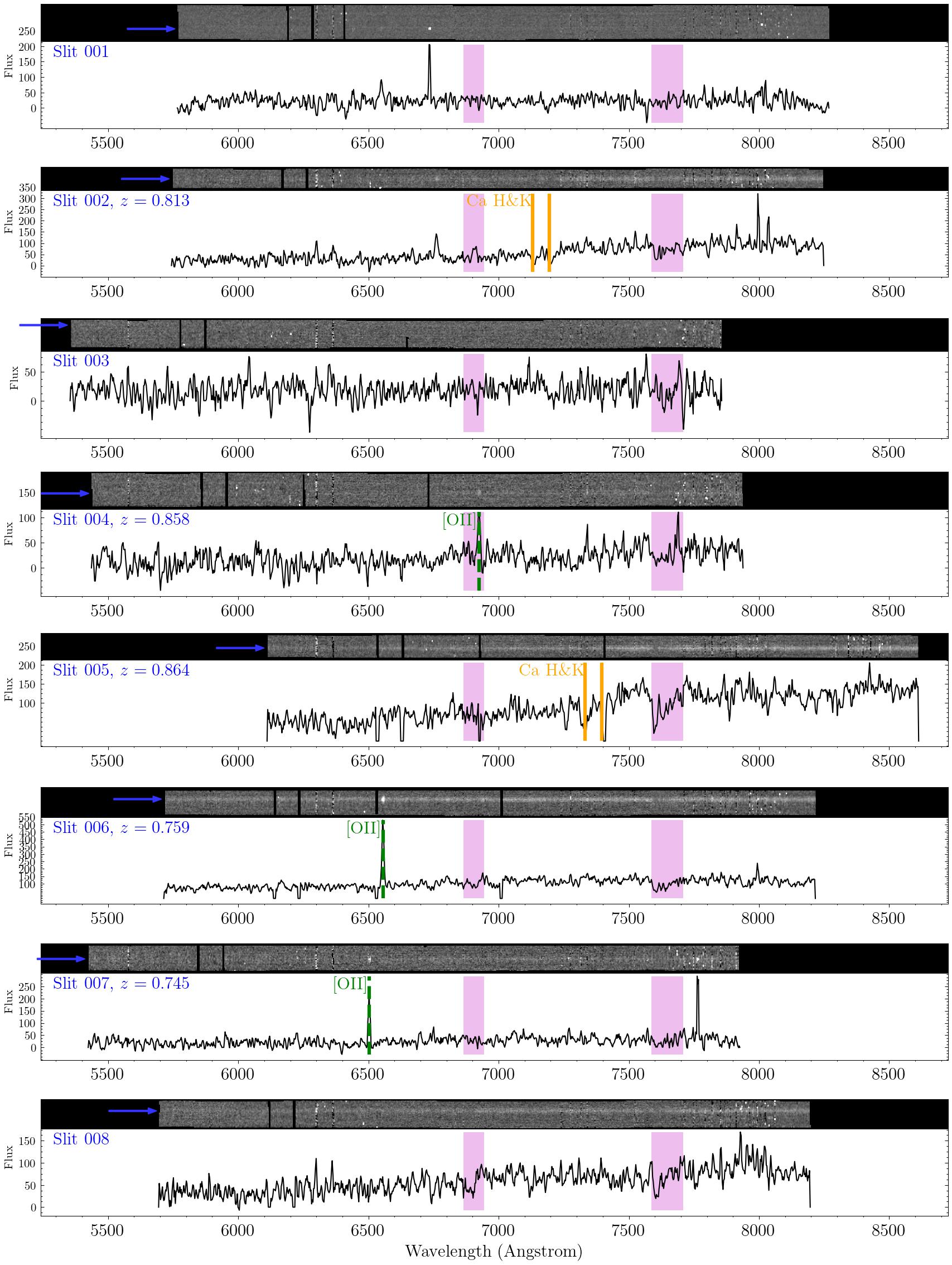
Figure 8: Galaxy Spectra of Slit #1–8.

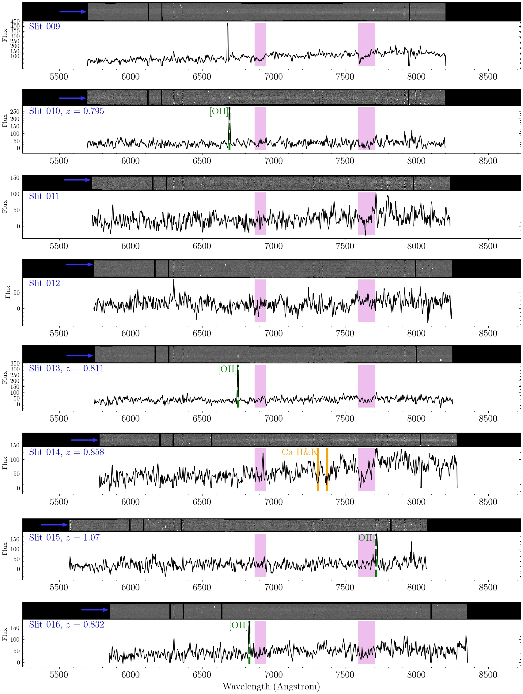
Figure 9: Galaxy Spectra of Slit #9–16.

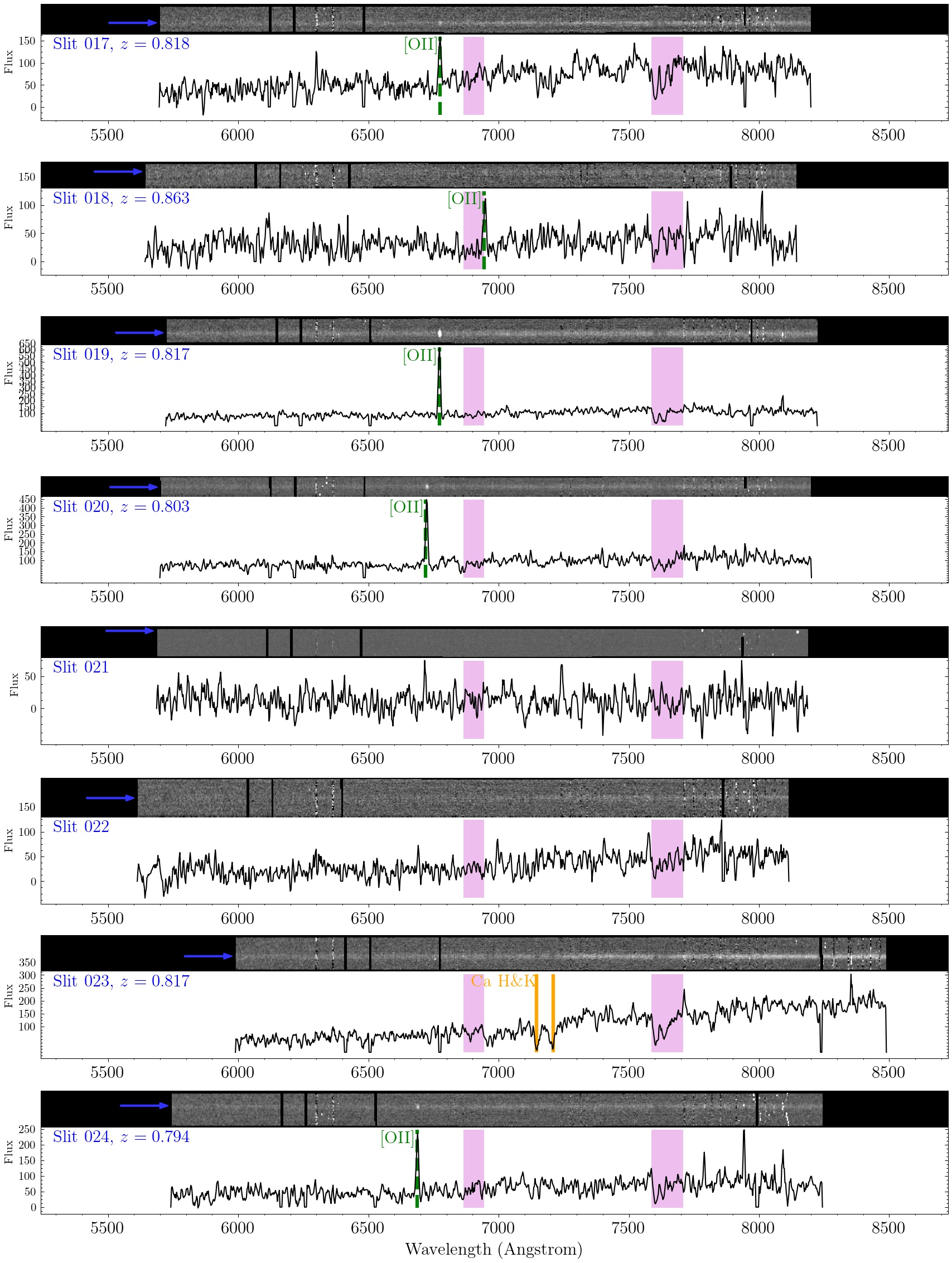
Figure 10: Galaxy Spectra of Slit #17–24.

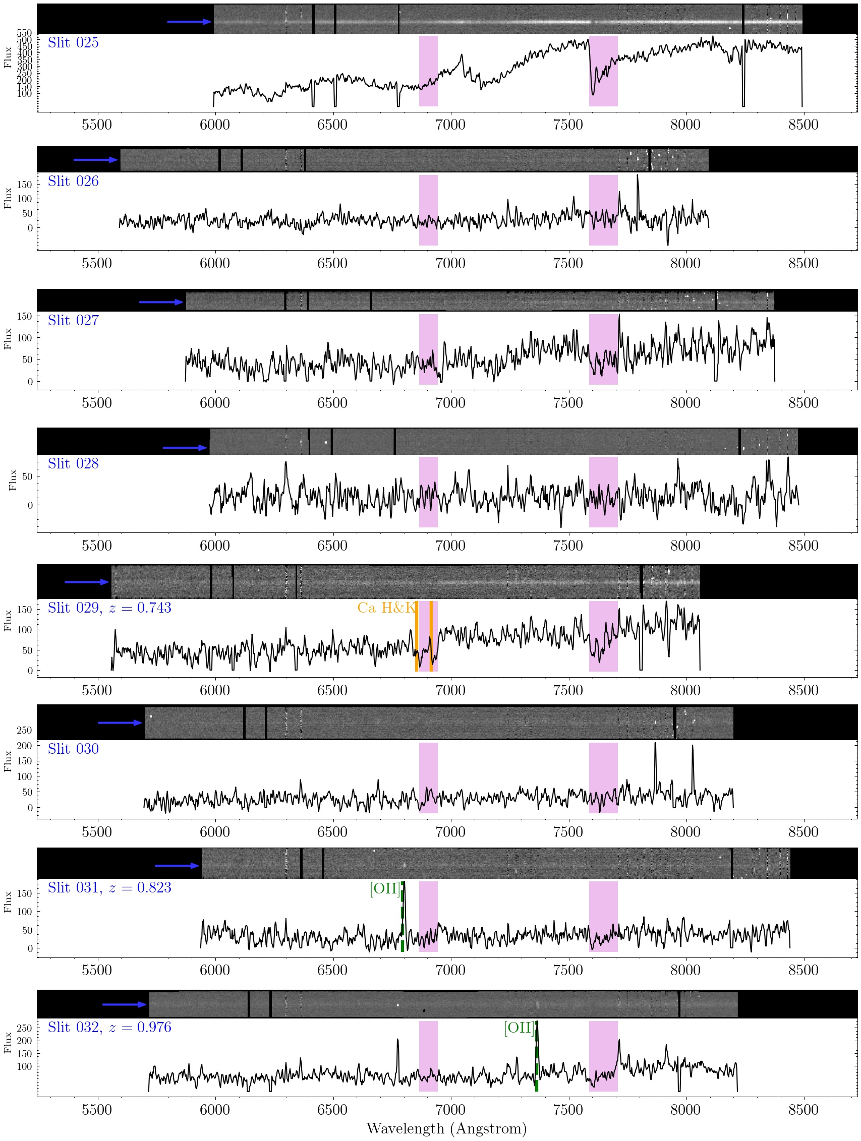
Figure 11: Galaxy Spectra of Slit #25–32.

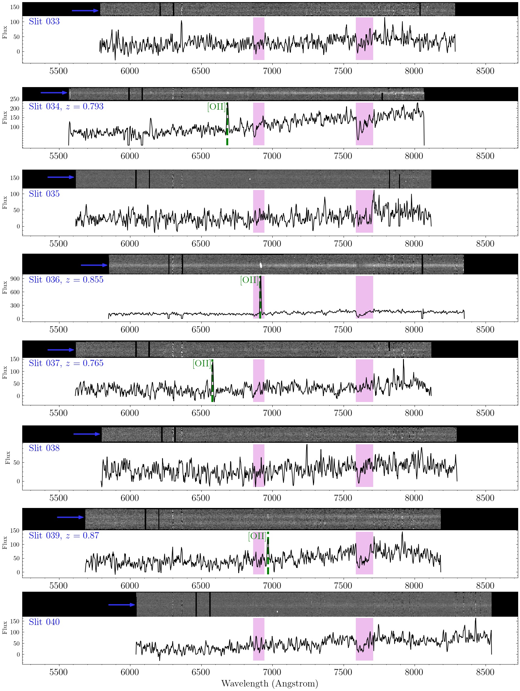
Figure 12: Galaxy Spectra of Slit #33–40.

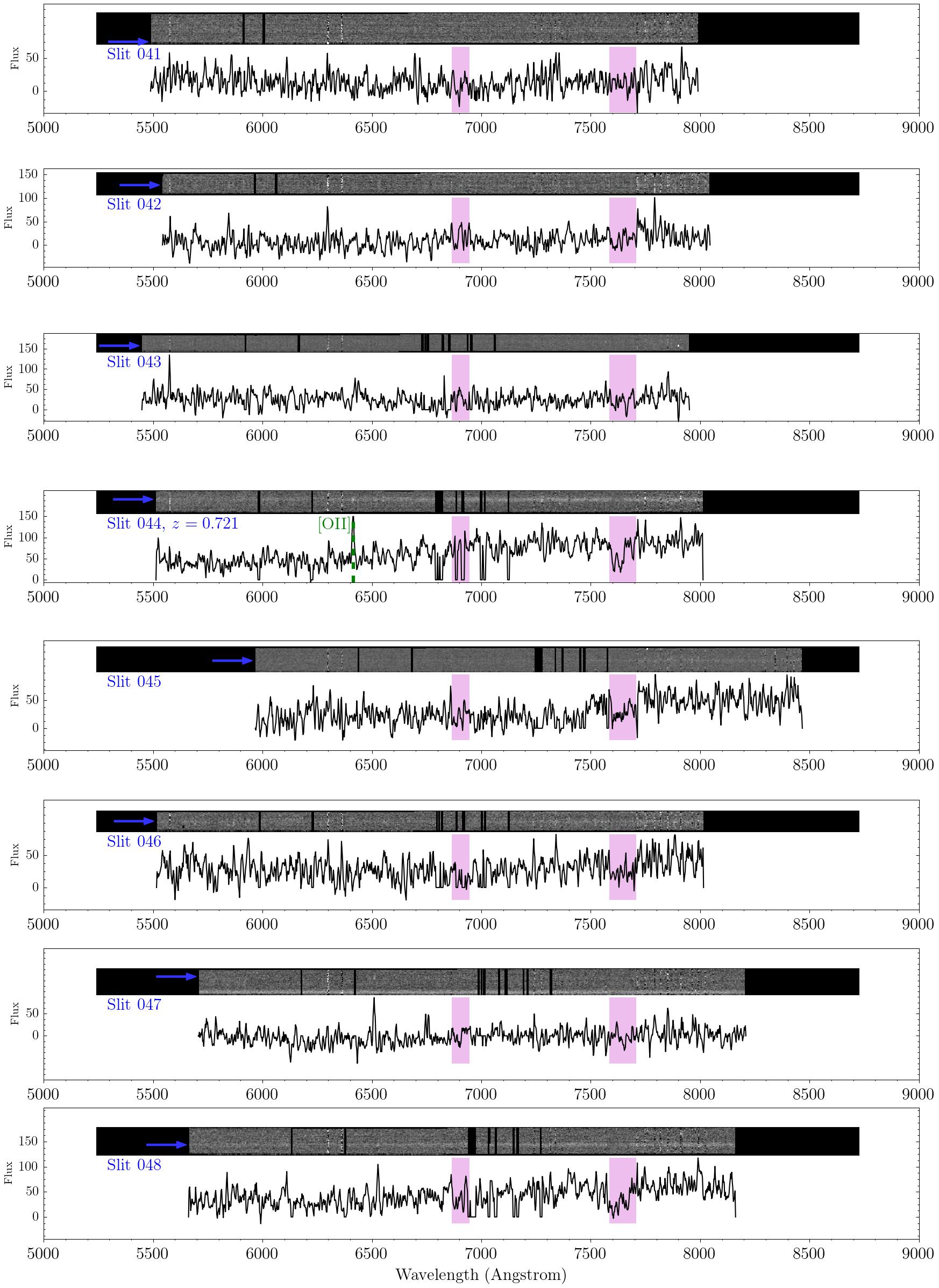
Figure 13: Galaxy Spectra of Slit #41–48.

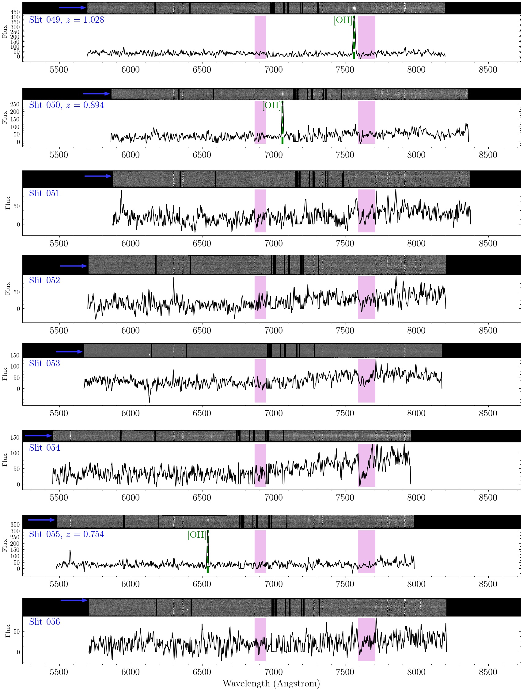
Figure 14: Galaxy Spectra of Slit #49–56.

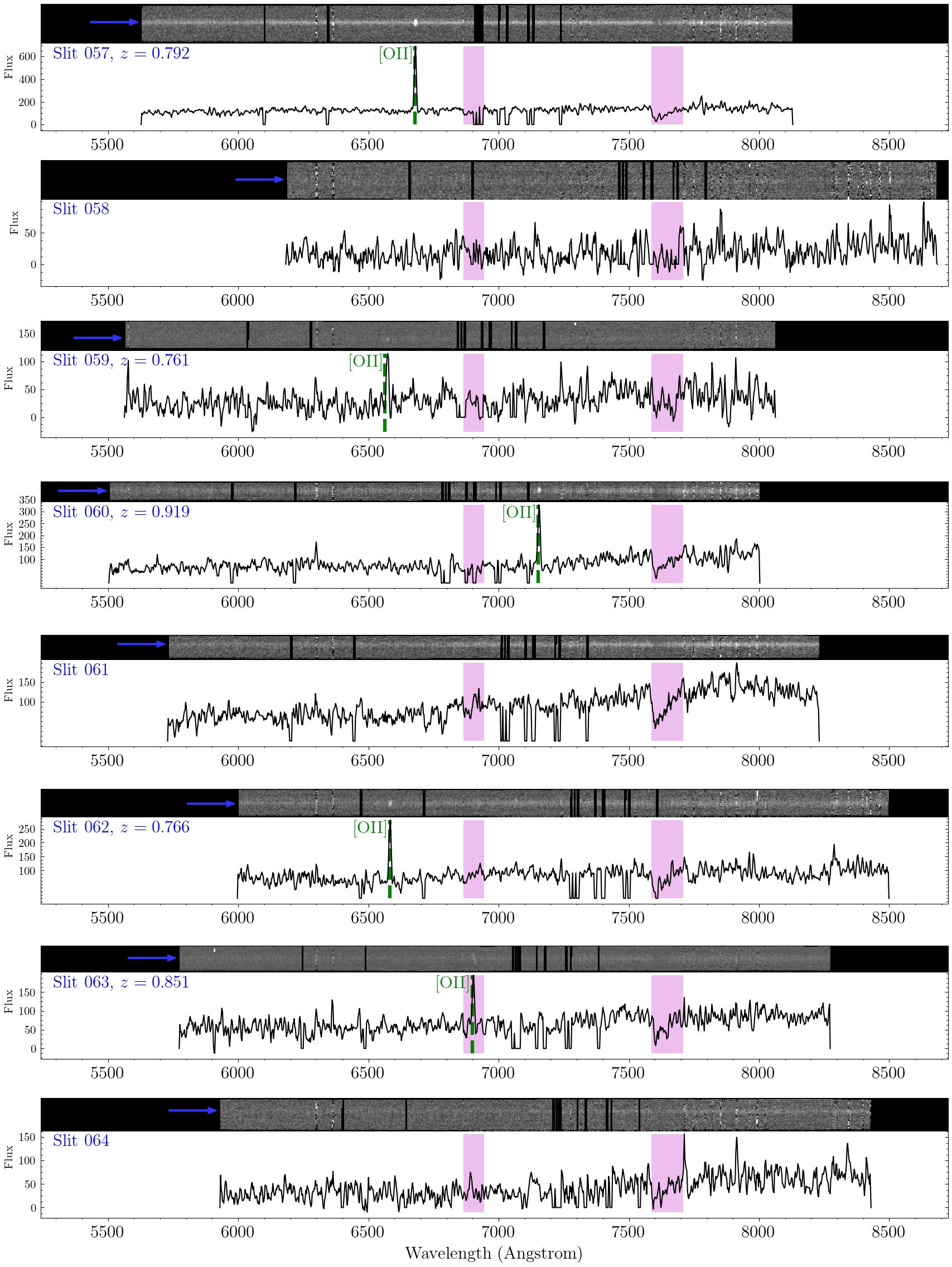
Figure 15: Galaxy Spectra of Slit #57–64.

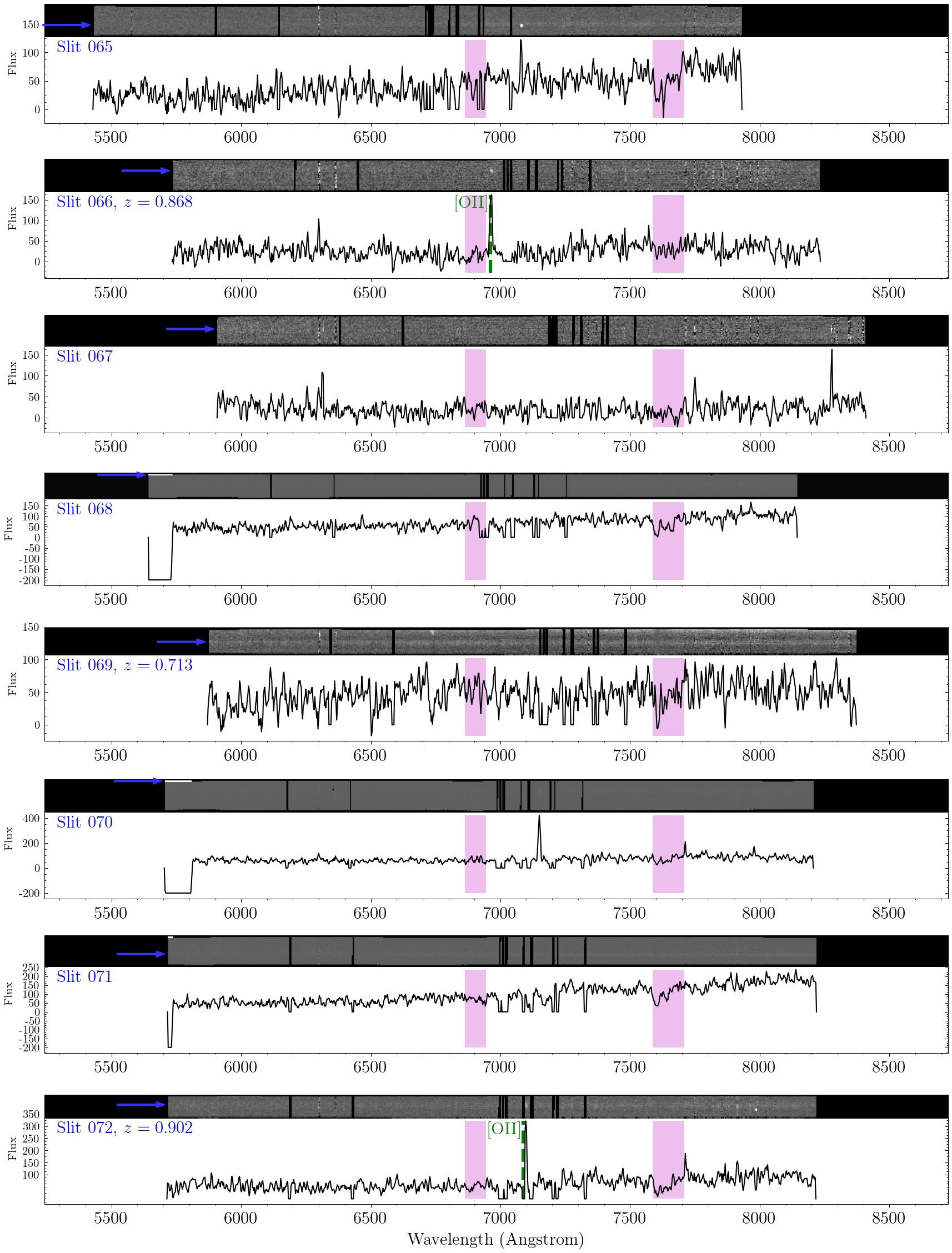
Figure 16: Galaxy Spectra of Slit #65–72.

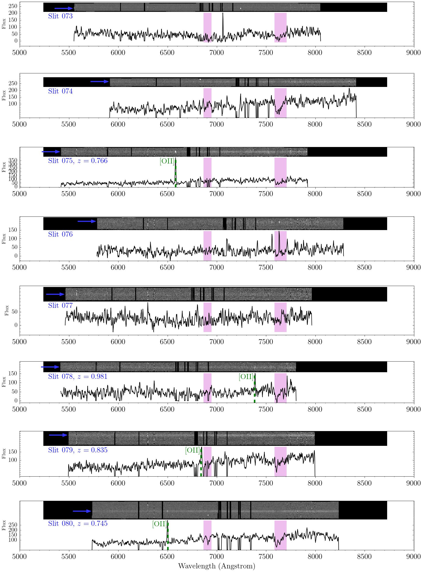
Figure 17: Galaxy Spectra of Slit #73–80.

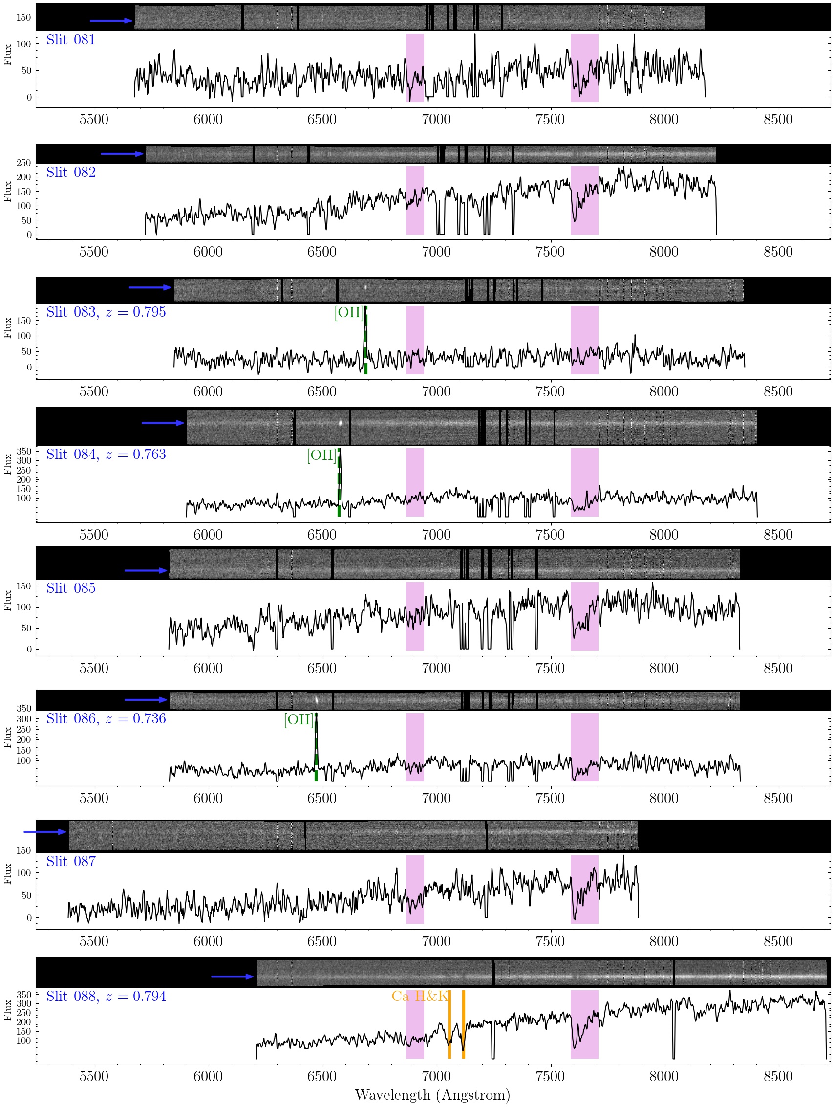
Figure 18: Galaxy Spectra of Slit #81–88.

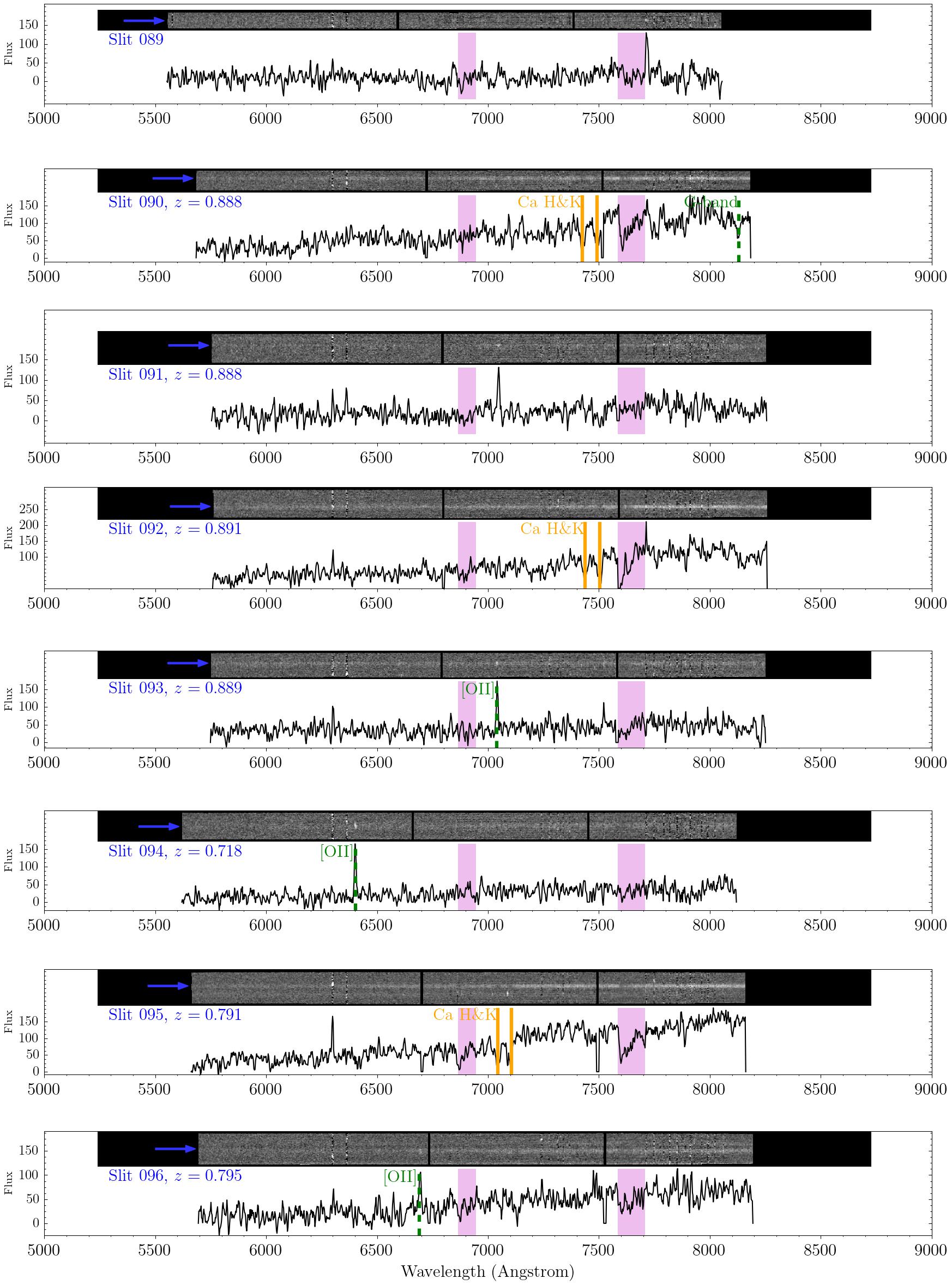
Figure 19: Galaxy Spectra of Slit #89–96.

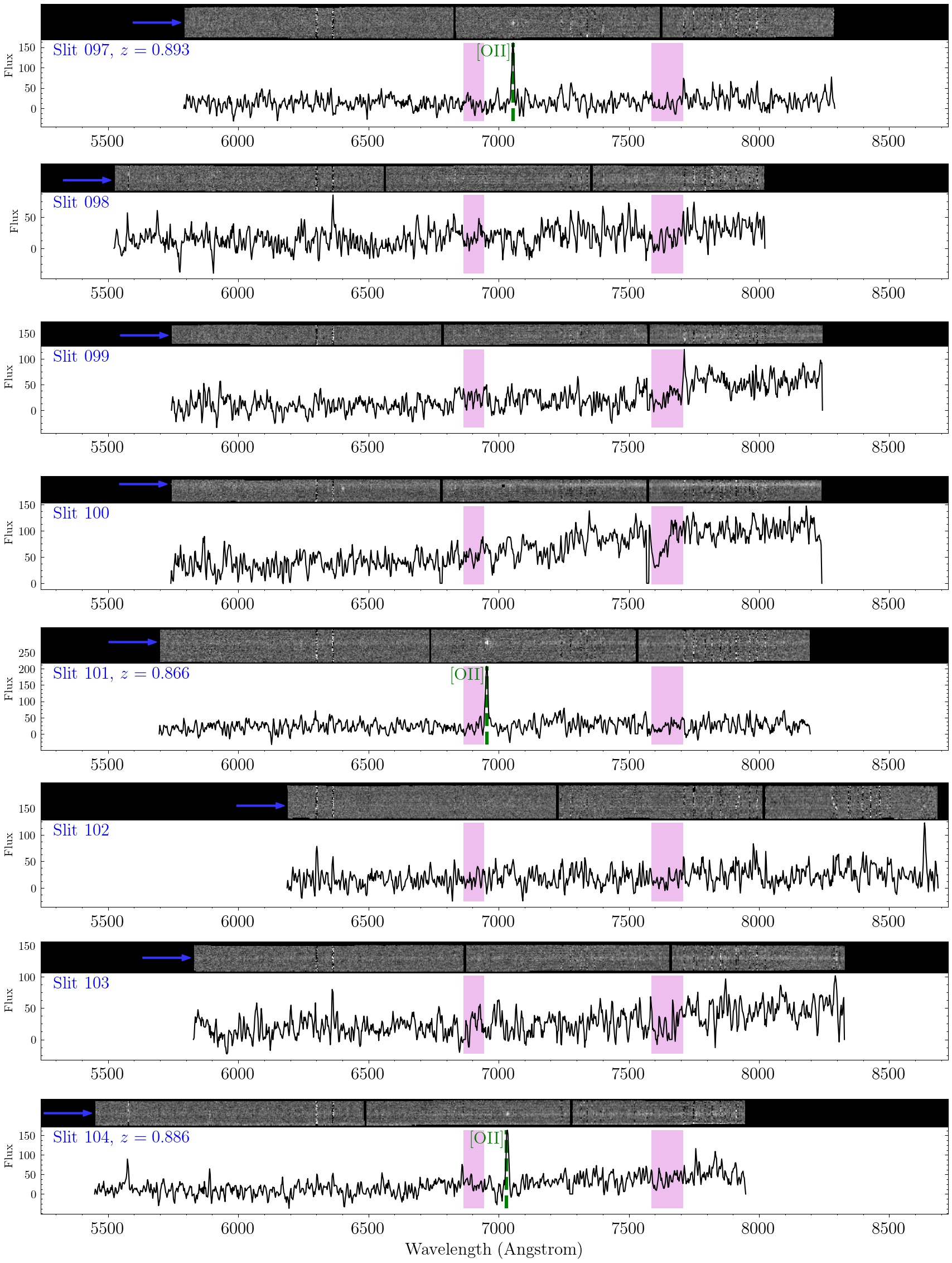
Figure 20: Galaxy Spectra of Slit #97–104.

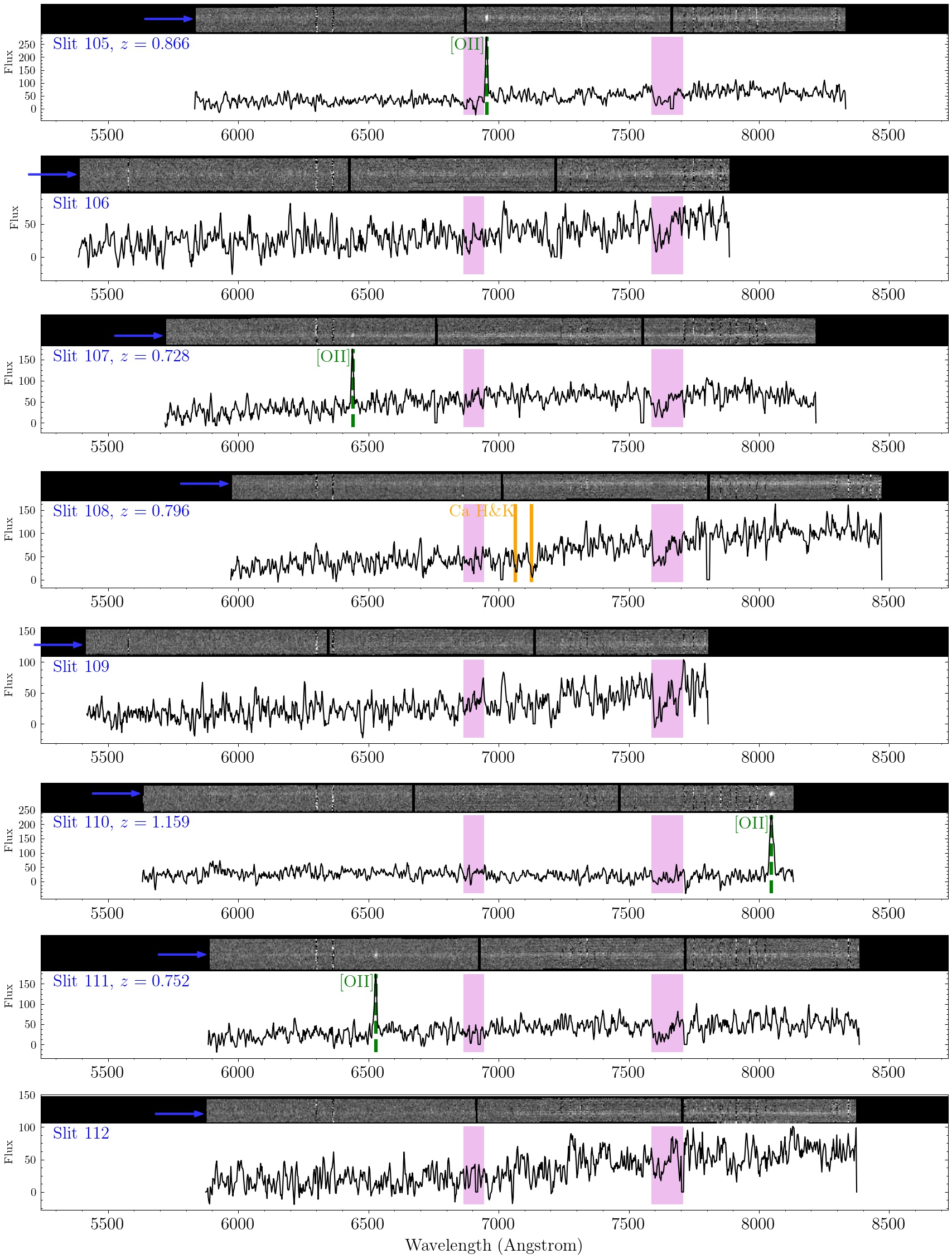
Figure 21: Galaxy Spectra of Slit #105–112.

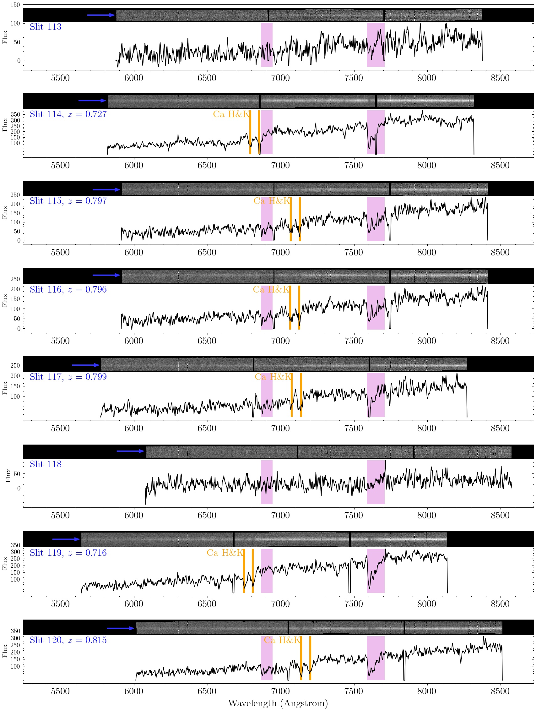
Figure 22: Galaxy Spectra of Slit #113–120.

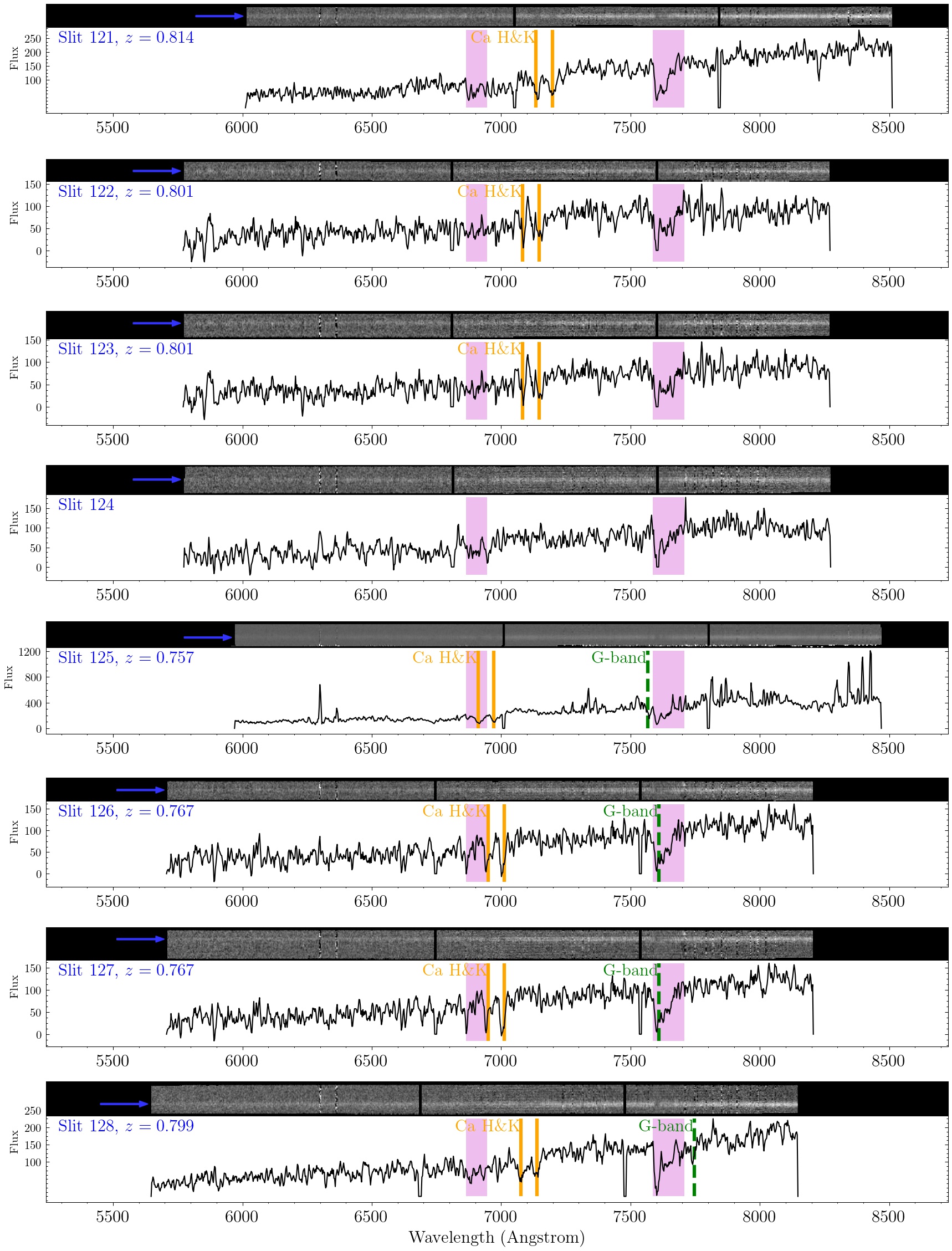
Figure 23: Galaxy Spectra of Slit #121–128.

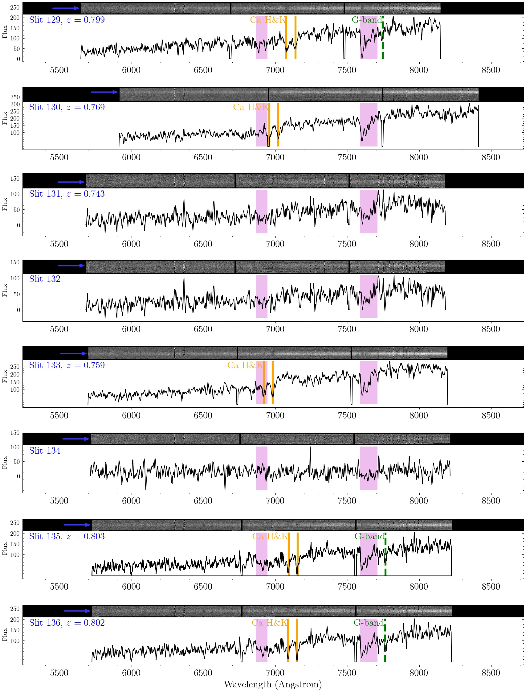
Figure 24: Galaxy Spectra of Slit #129–136.

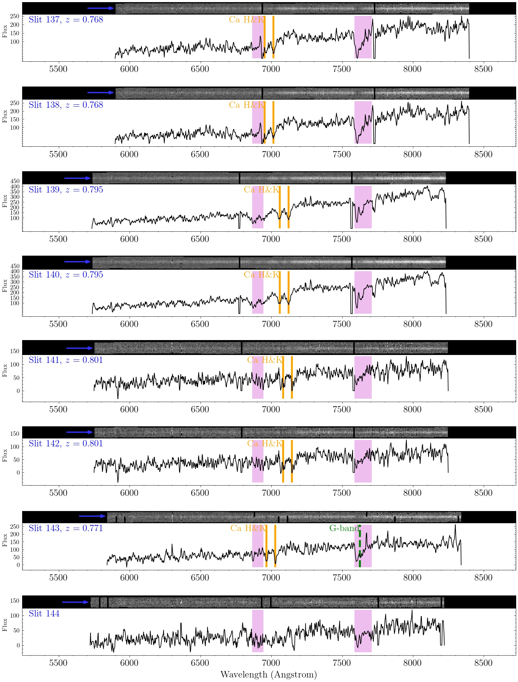
Figure 25: Galaxy Spectra of Slit #137–144.

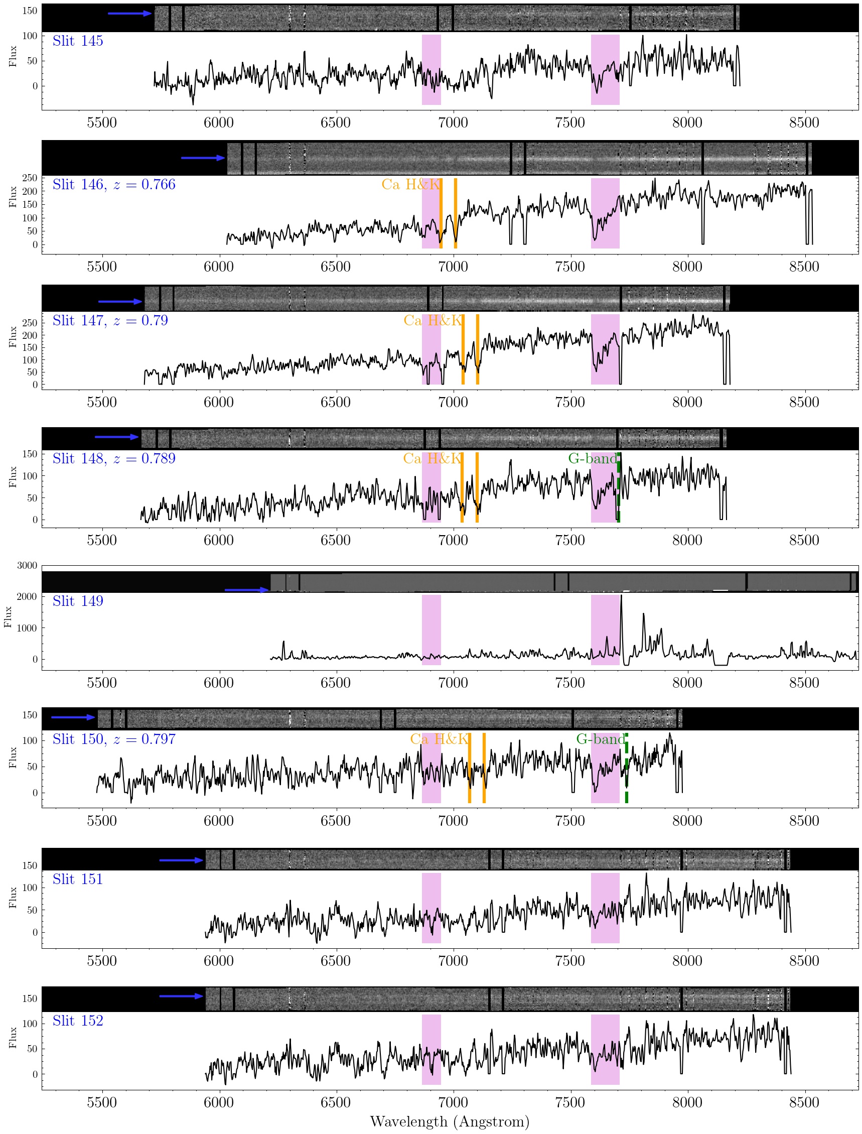
Figure 26: Galaxy Spectra of Slit #145–152.

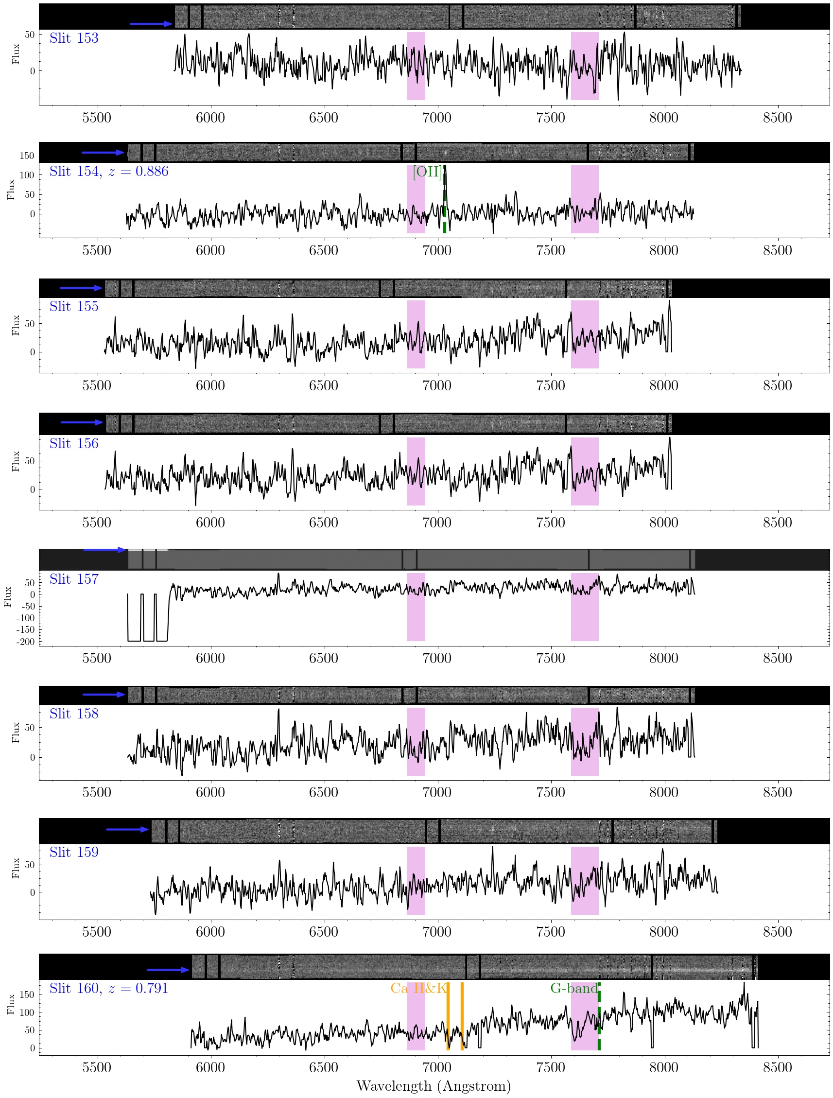
Figure 27: Galaxy Spectra of Slit #153–160.

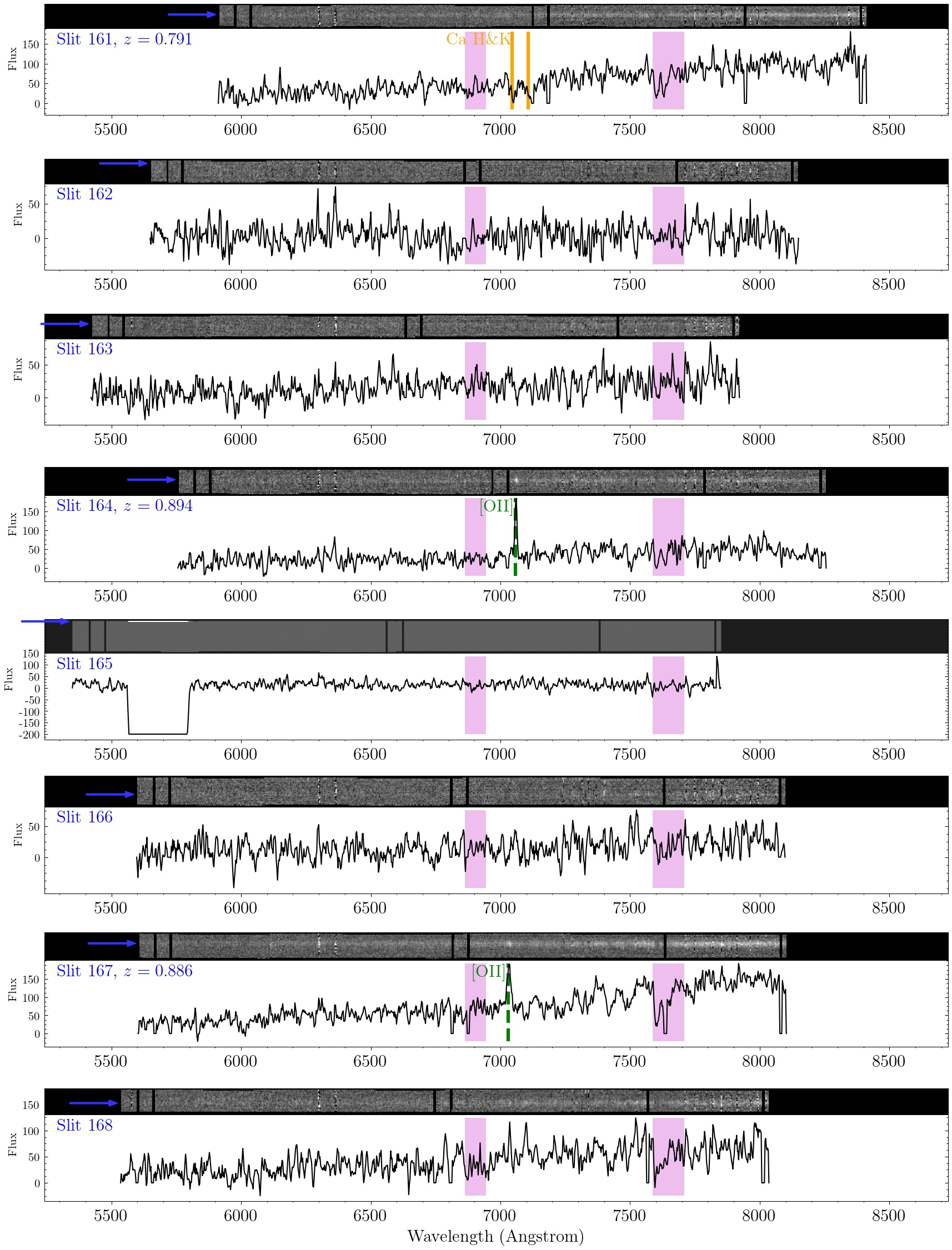
Figure 28: Galaxy Spectra of Slit #161–168.

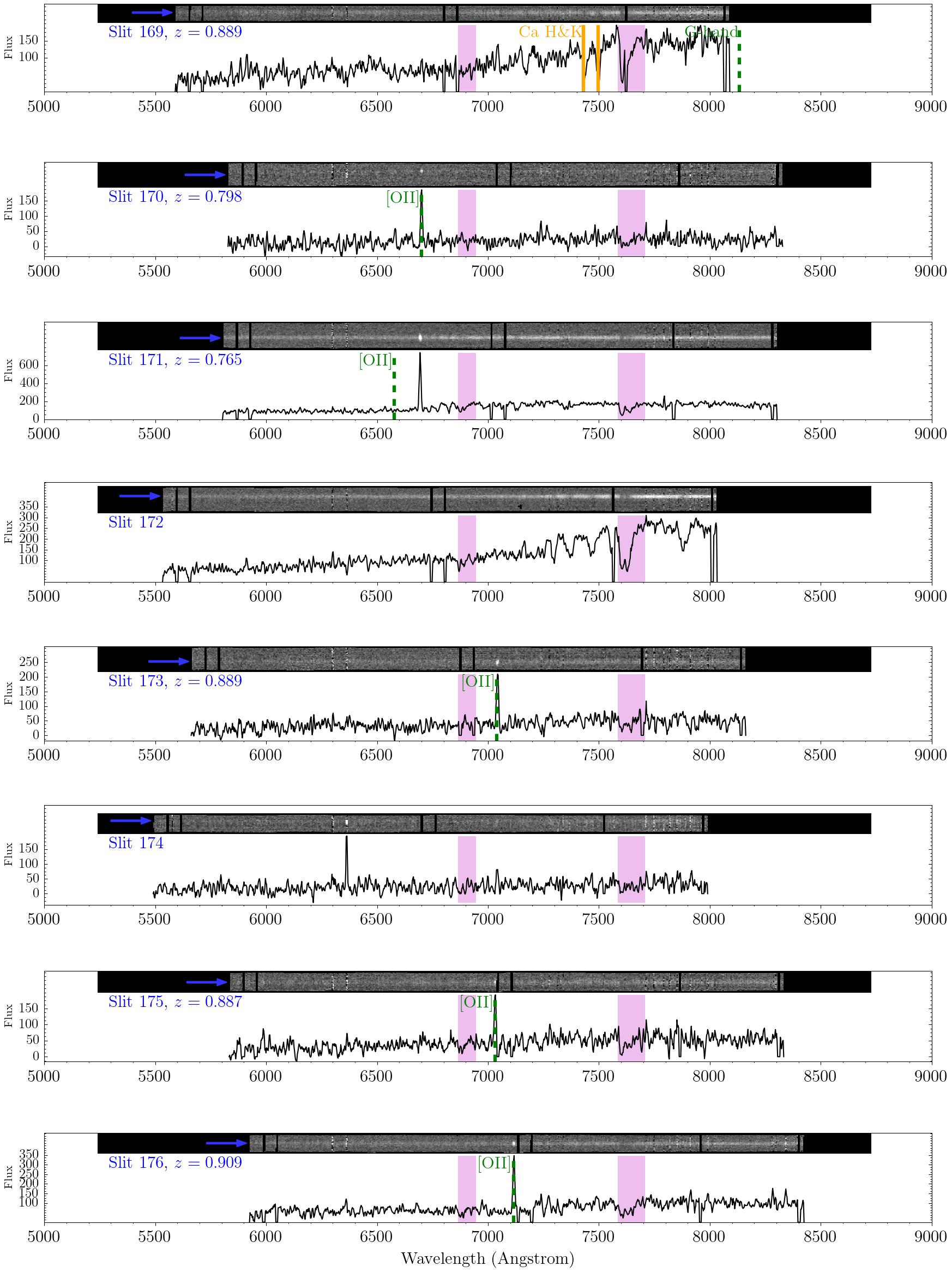
Figure 29: Galaxy Spectra of Slit #169–176.

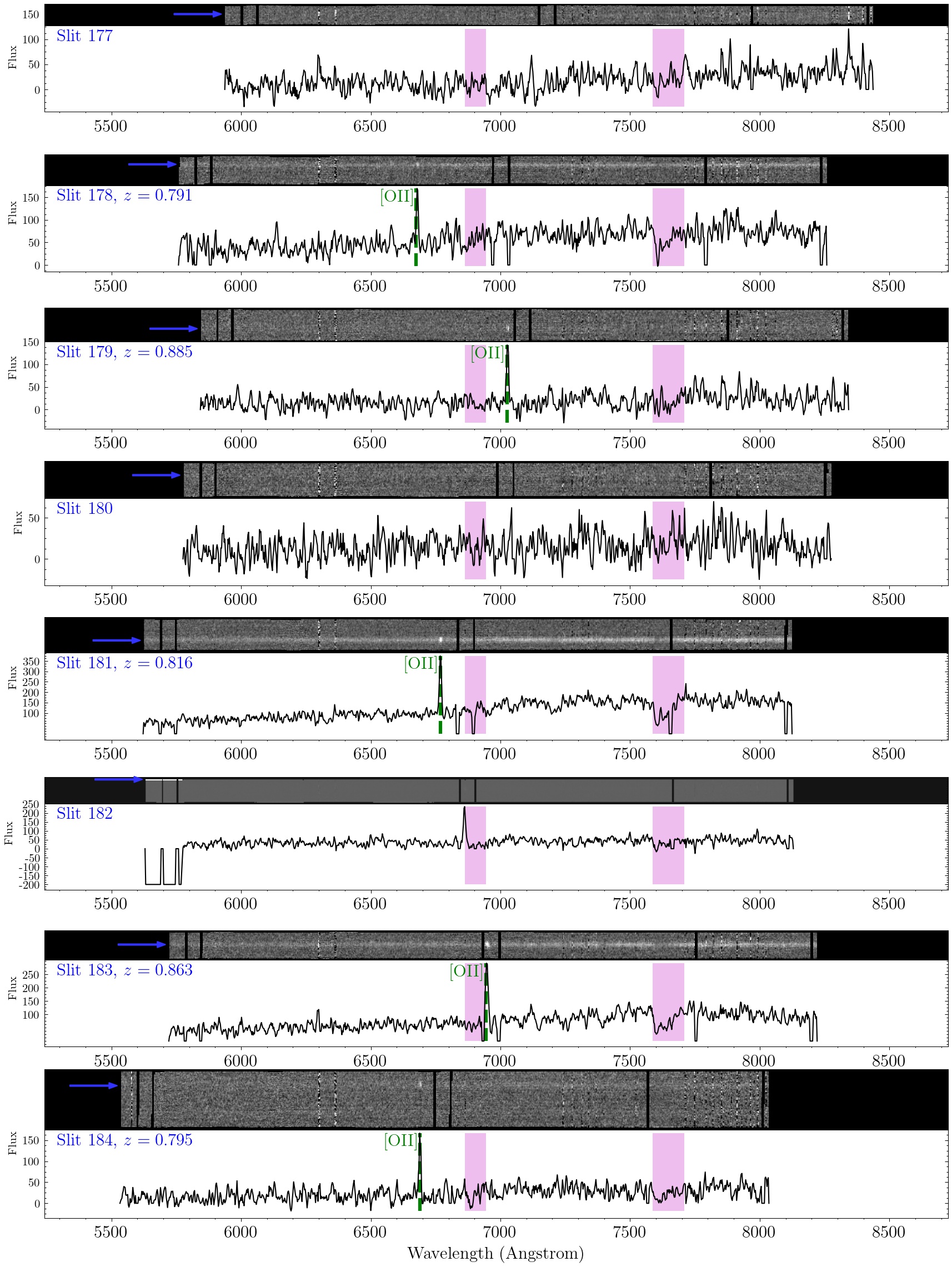
Figure 30: Galaxy Spectra of Slit #177–184.

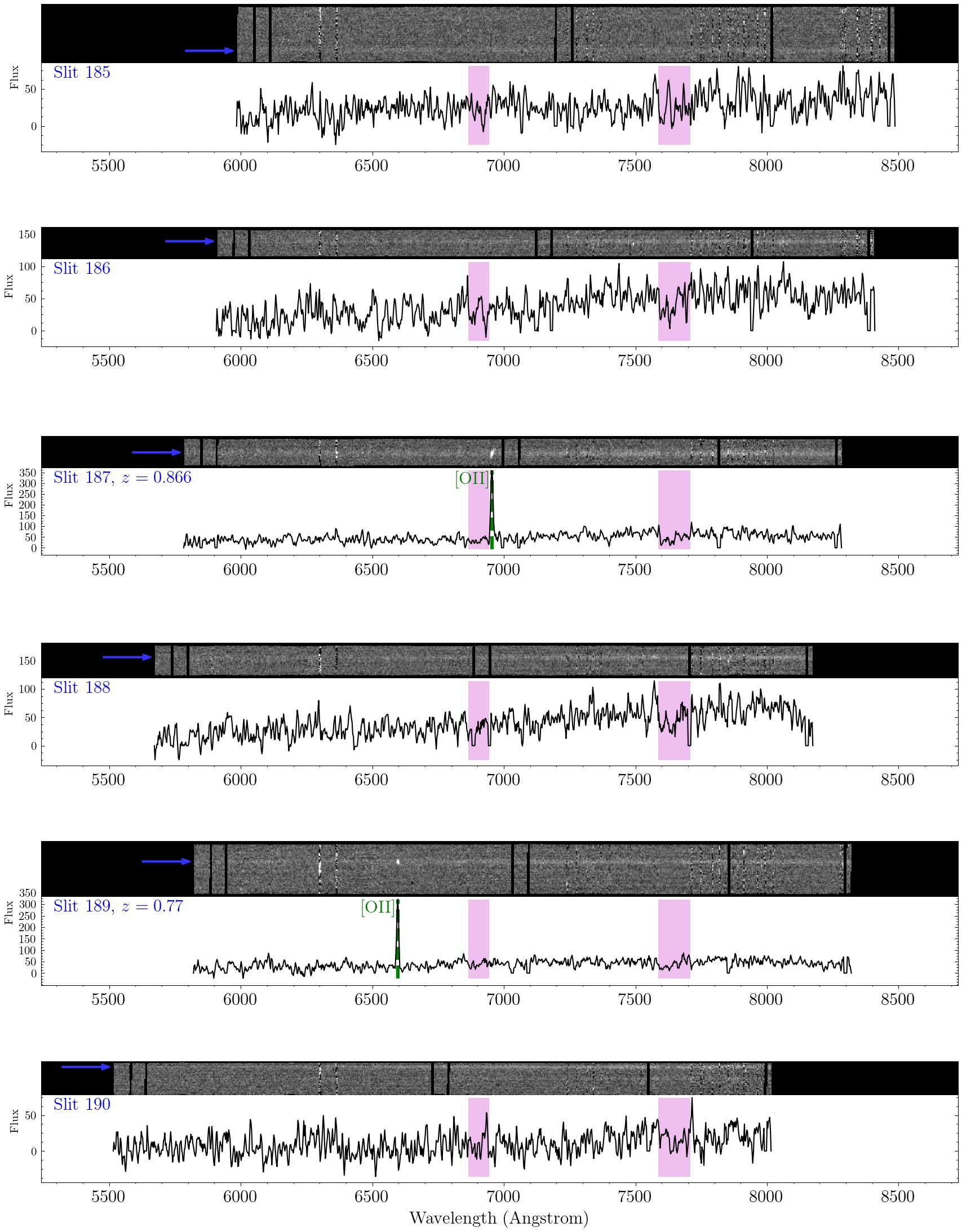
Figure 31: Galaxy Spectra of Slit #185–190.

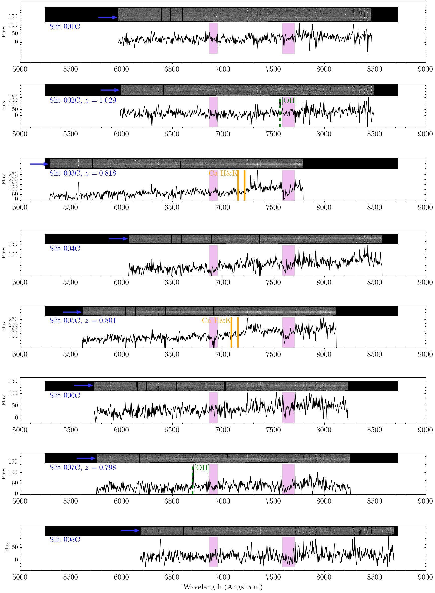
Figure 32: Galaxy Spectra of Slit #1C–8C.

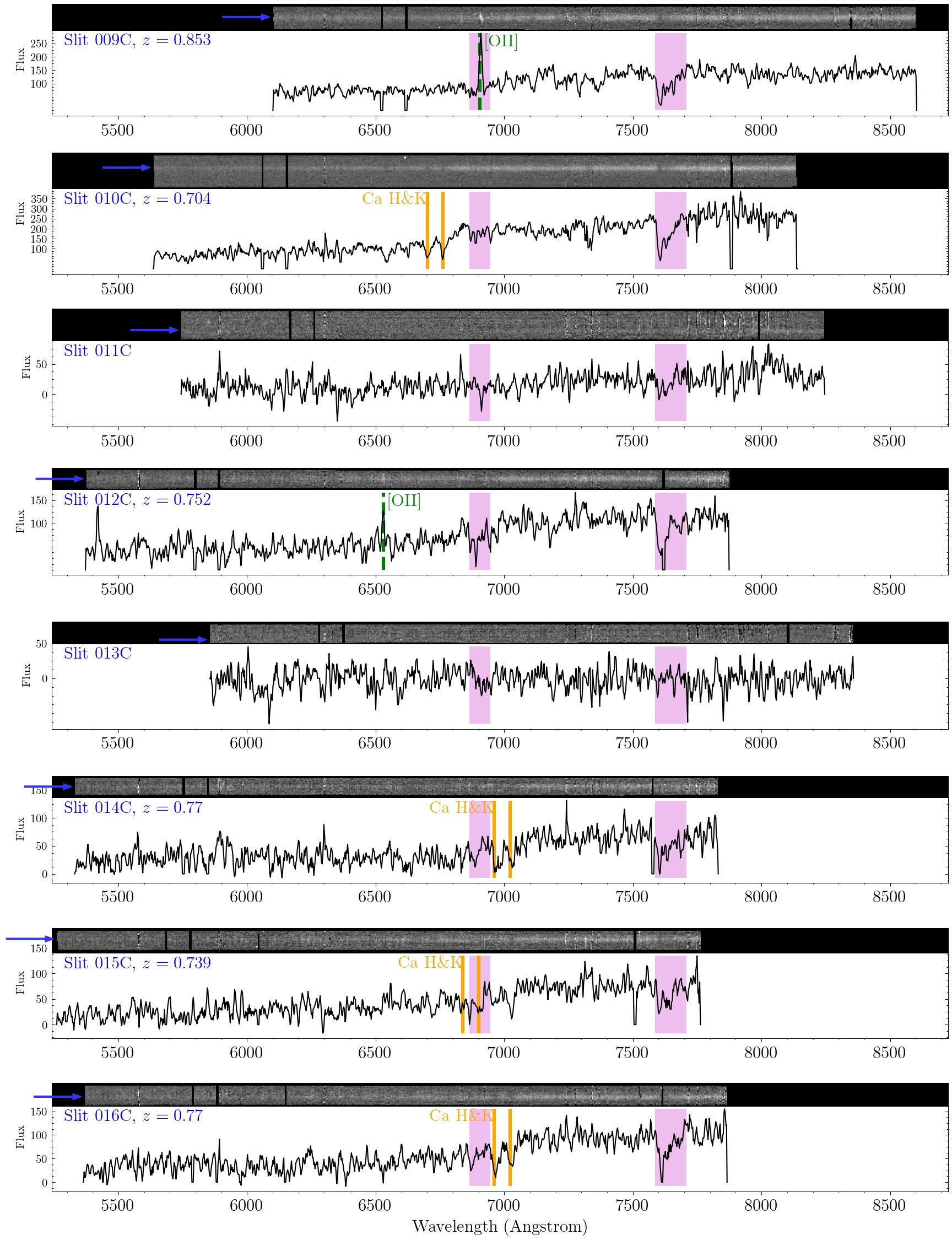
Figure 33: Galaxy Spectra of Slit #9C–16C.

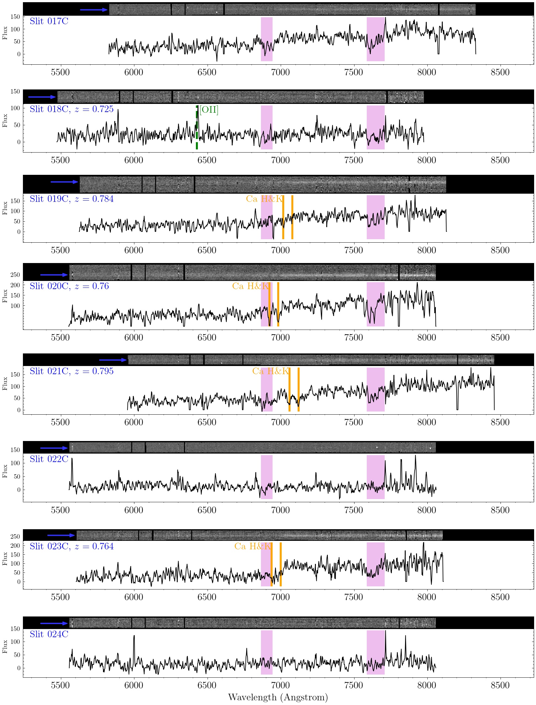
Figure 34: Galaxy Spectra of Slit #17C–24C.

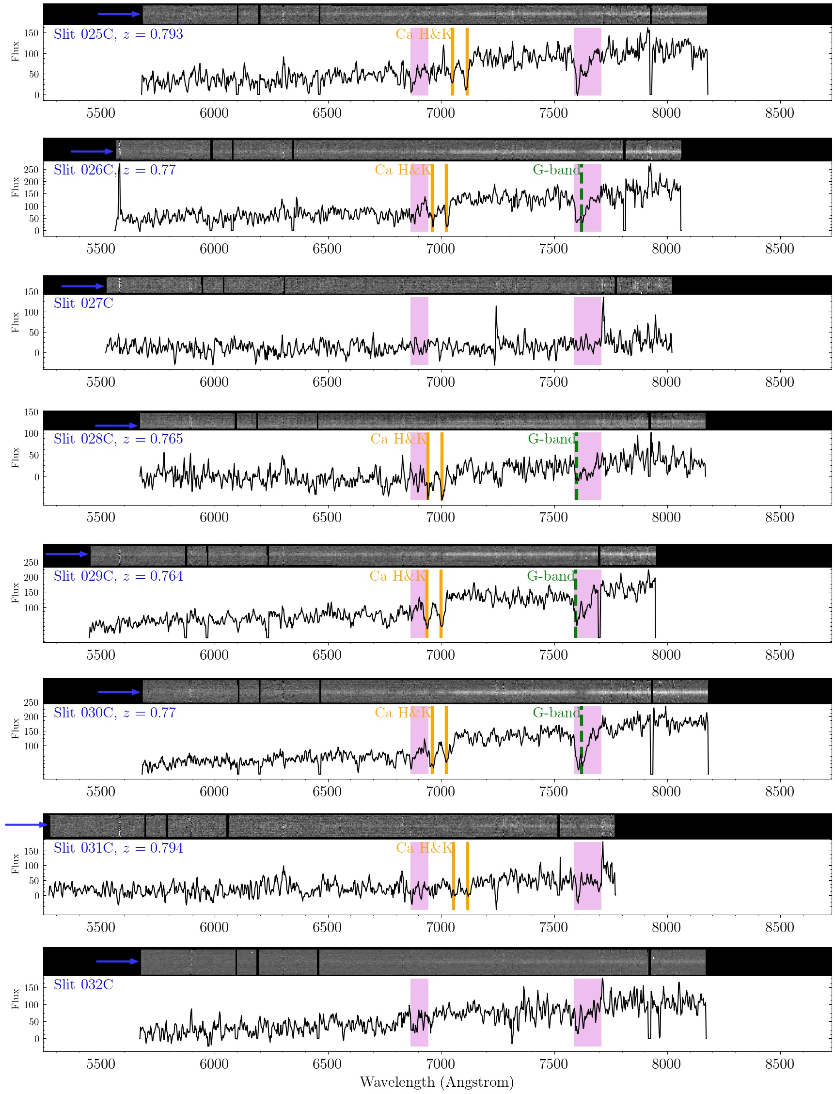
Figure 35: Galaxy Spectra of Slit #25C–32C.

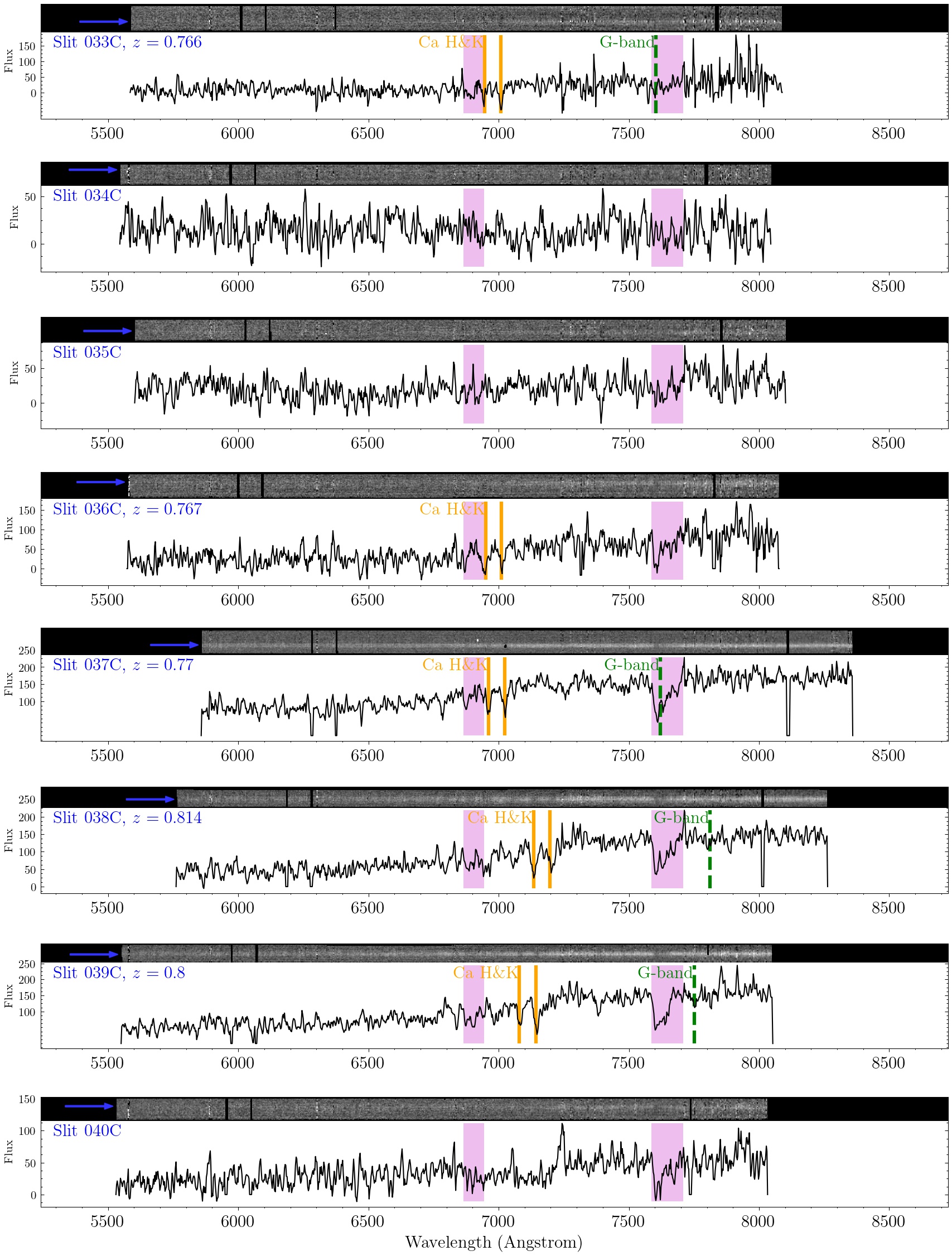
Figure 36: Galaxy Spectra of Slit #33C–40C.

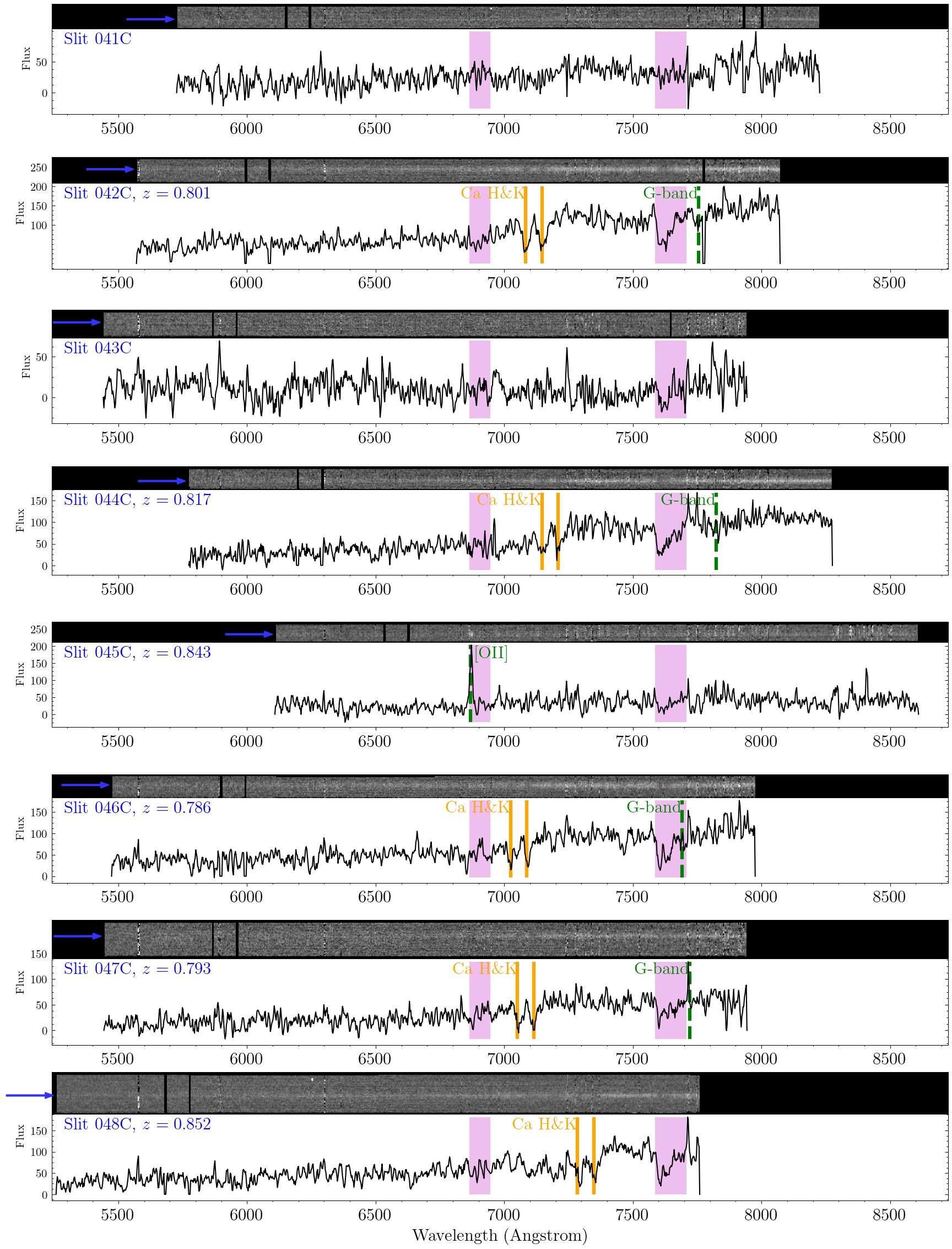
Figure 37: Galaxy Spectra of Slit #41C–48C.

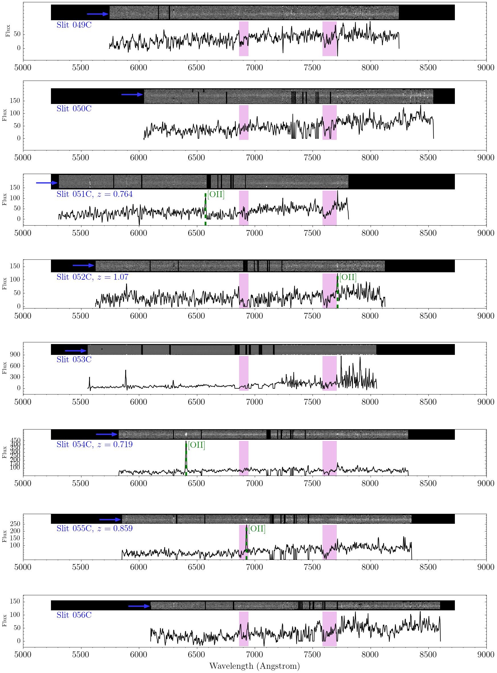
Figure 38: Galaxy Spectra of Slit #49C–56C.

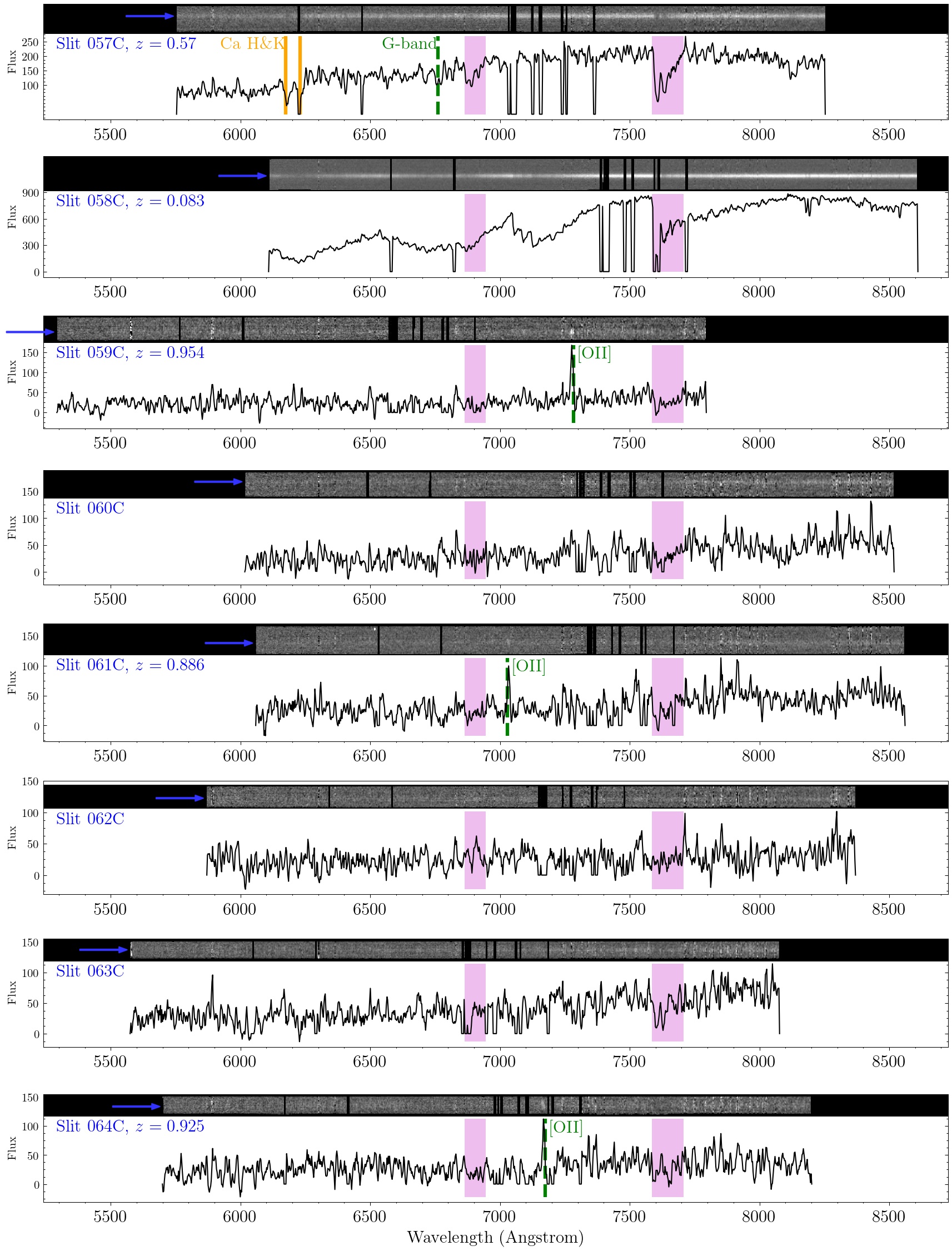
Figure 39: Galaxy Spectra of Slit #57C–64C.

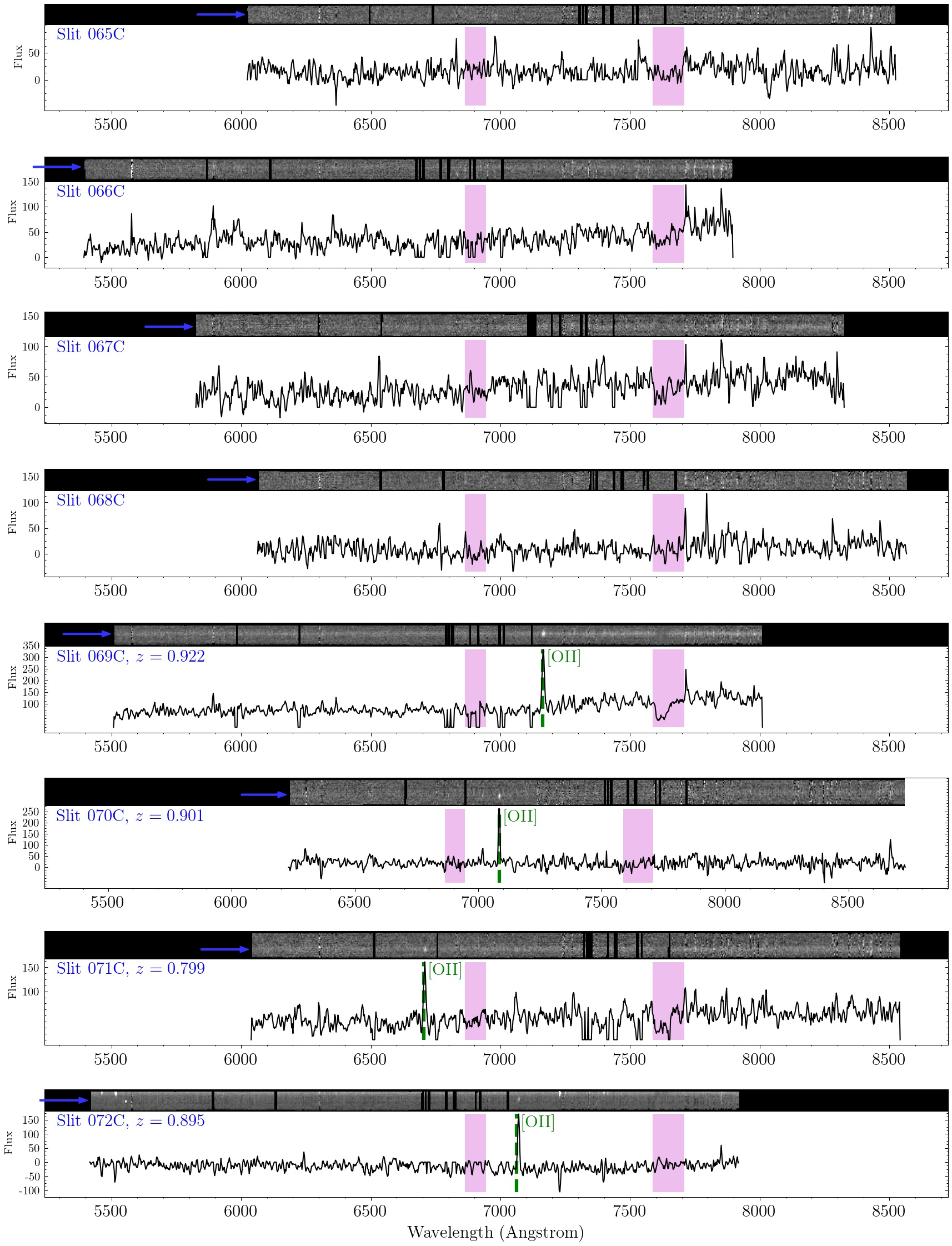
Figure 40: Galaxy Spectra of Slit #65C–72C.

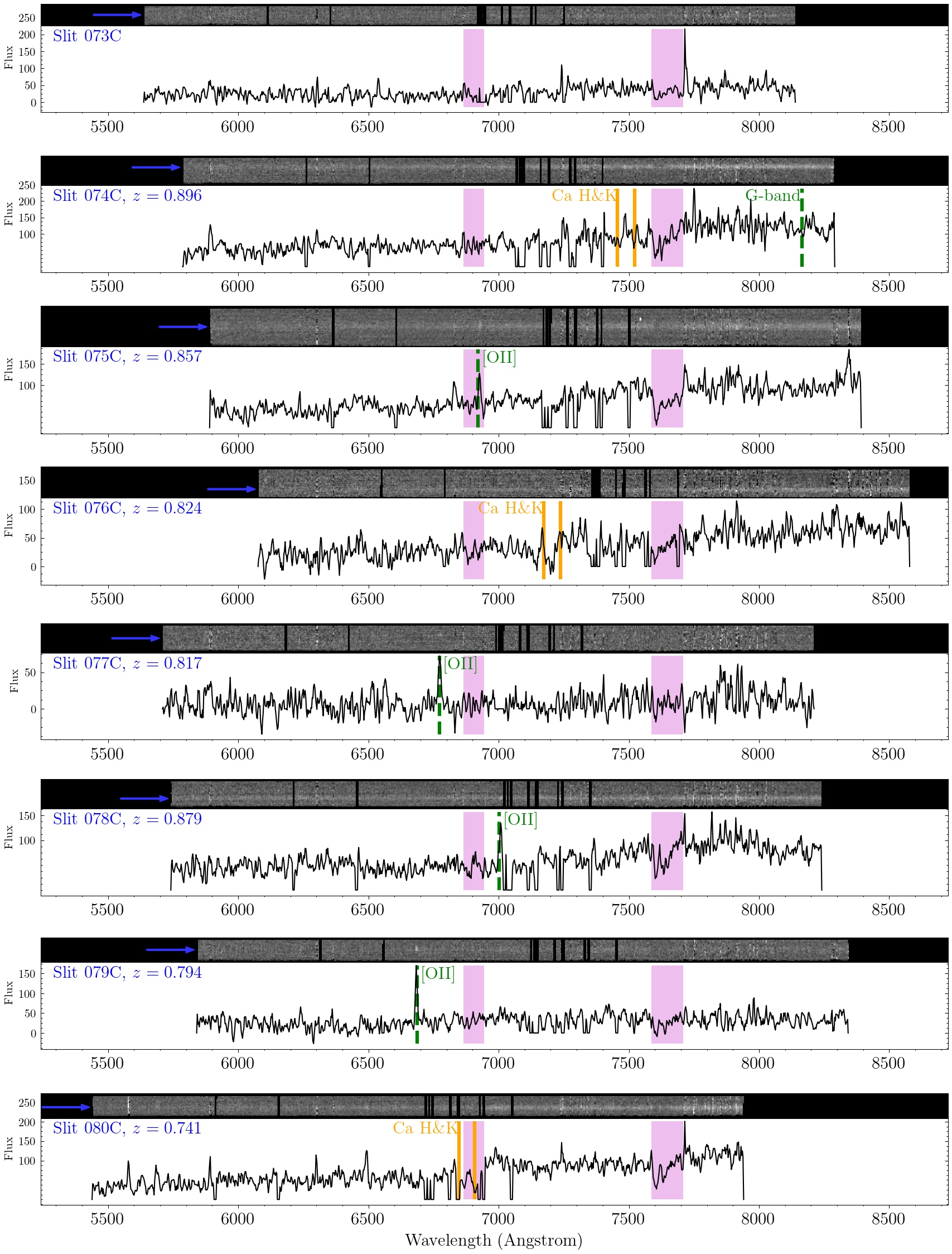
Figure 41: Galaxy Spectra of Slit #73C–80C.

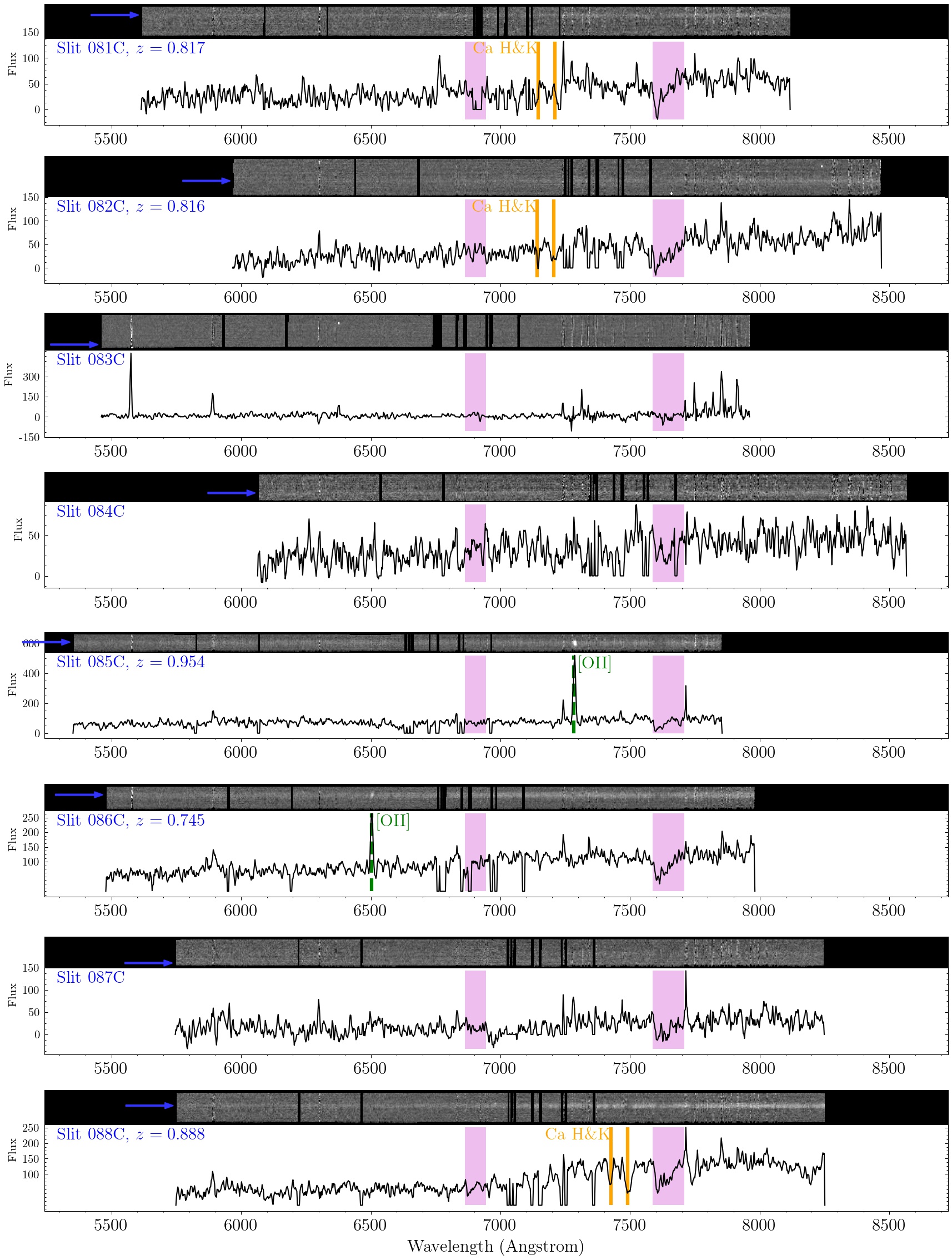
Figure 42: Galaxy Spectra of Slit #81C–88C.

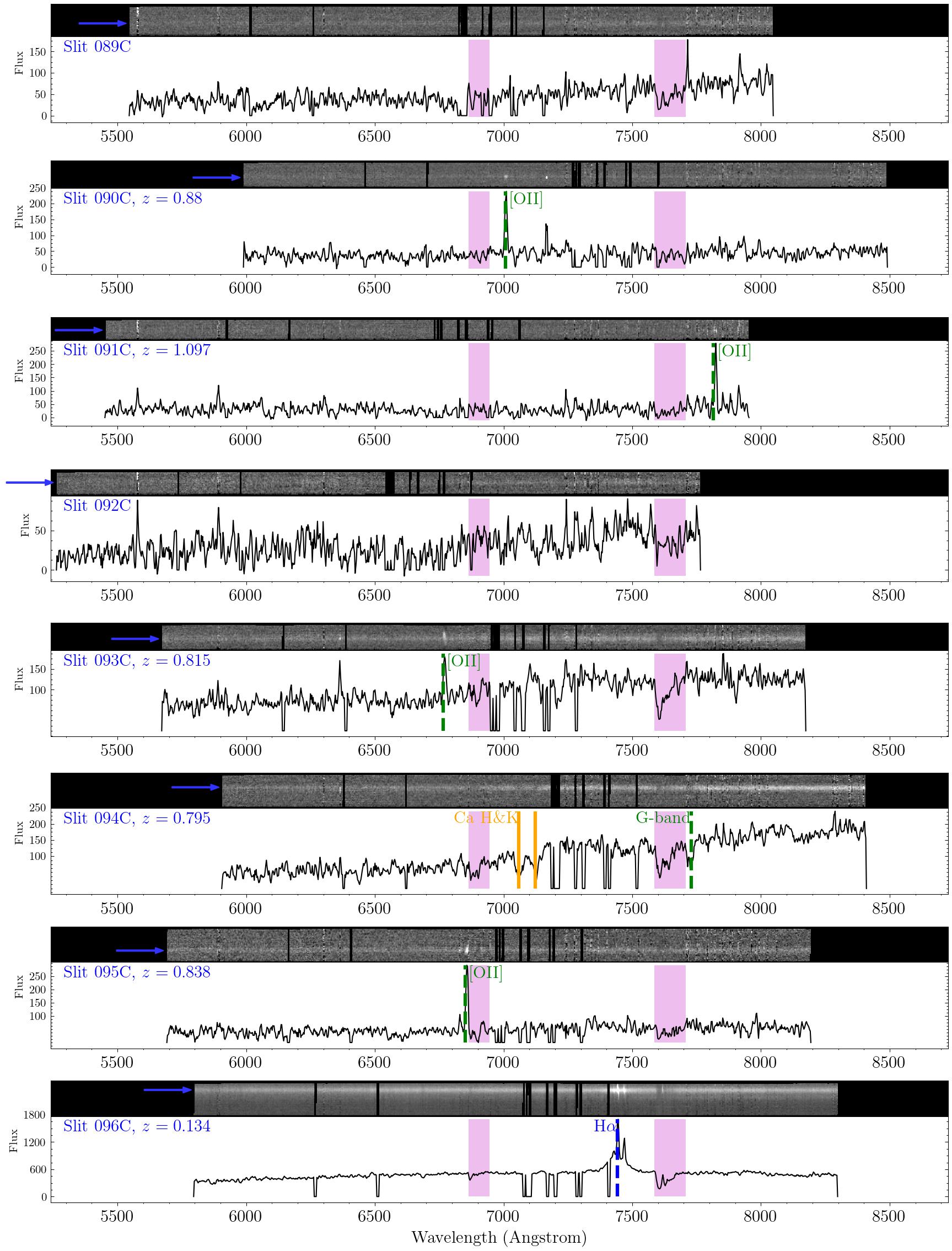
Figure 43: Galaxy Spectra of Slit #89C–96C.

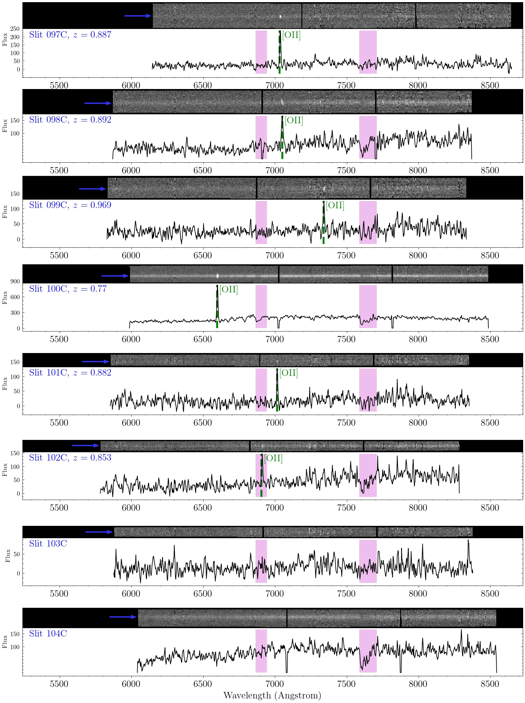
Figure 44: Galaxy Spectra of Slit #97C–104C.

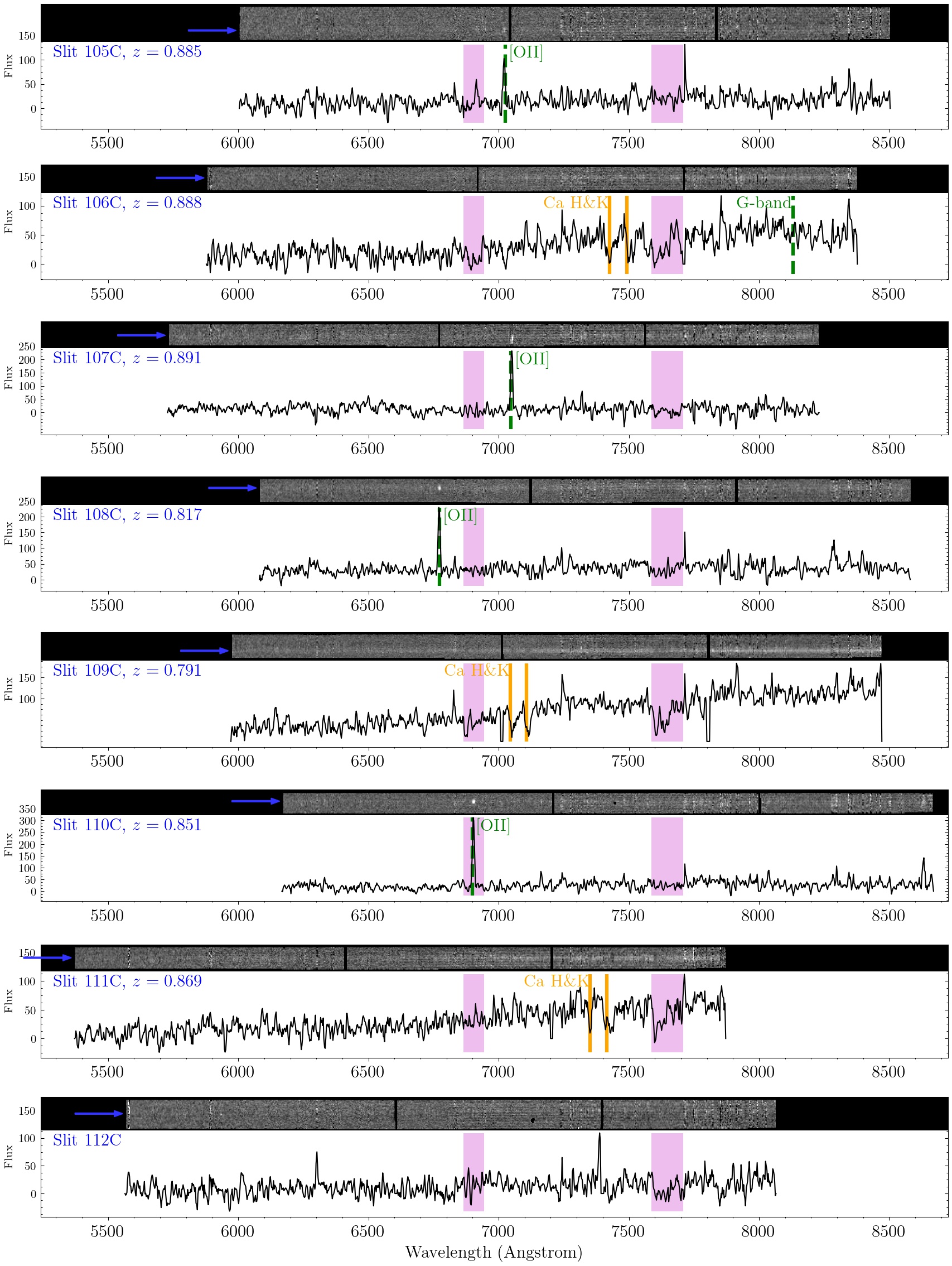
Figure 45: Galaxy Spectra of Slit #105C–112C.

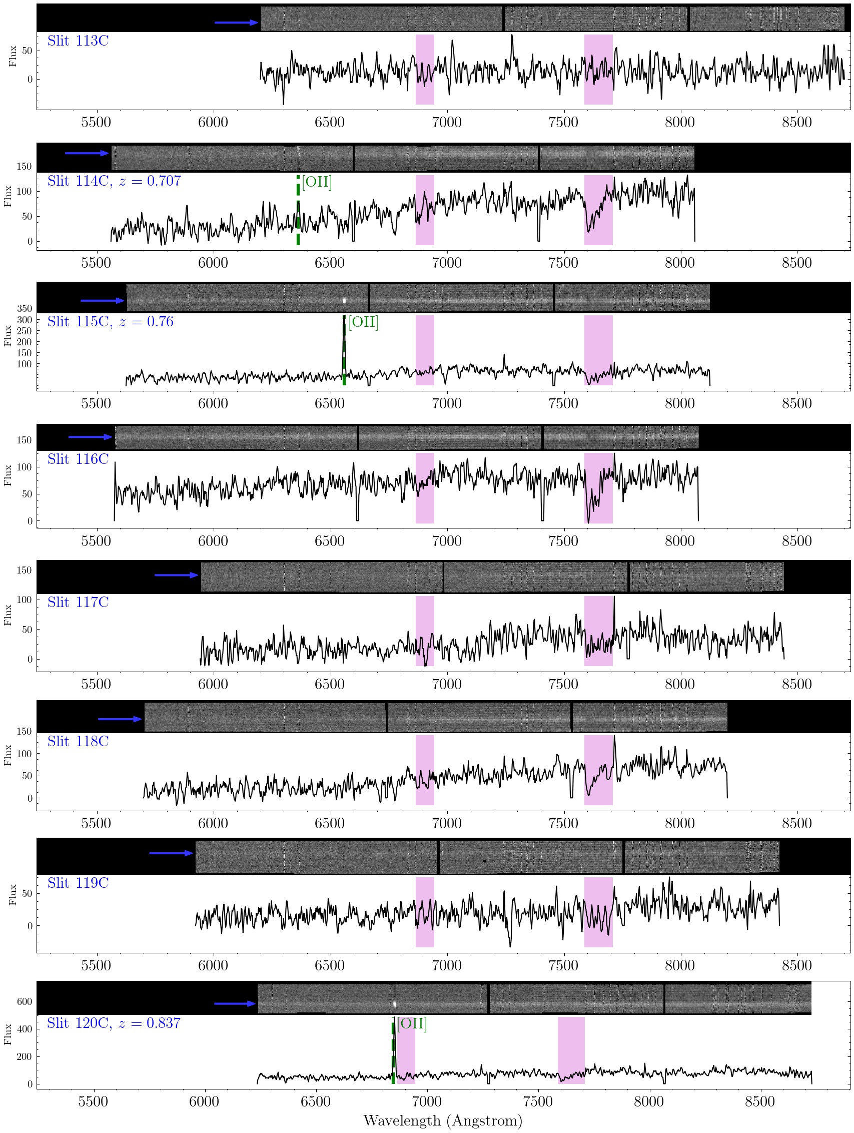
Figure 46: Galaxy Spectra of Slit #113C–120C.

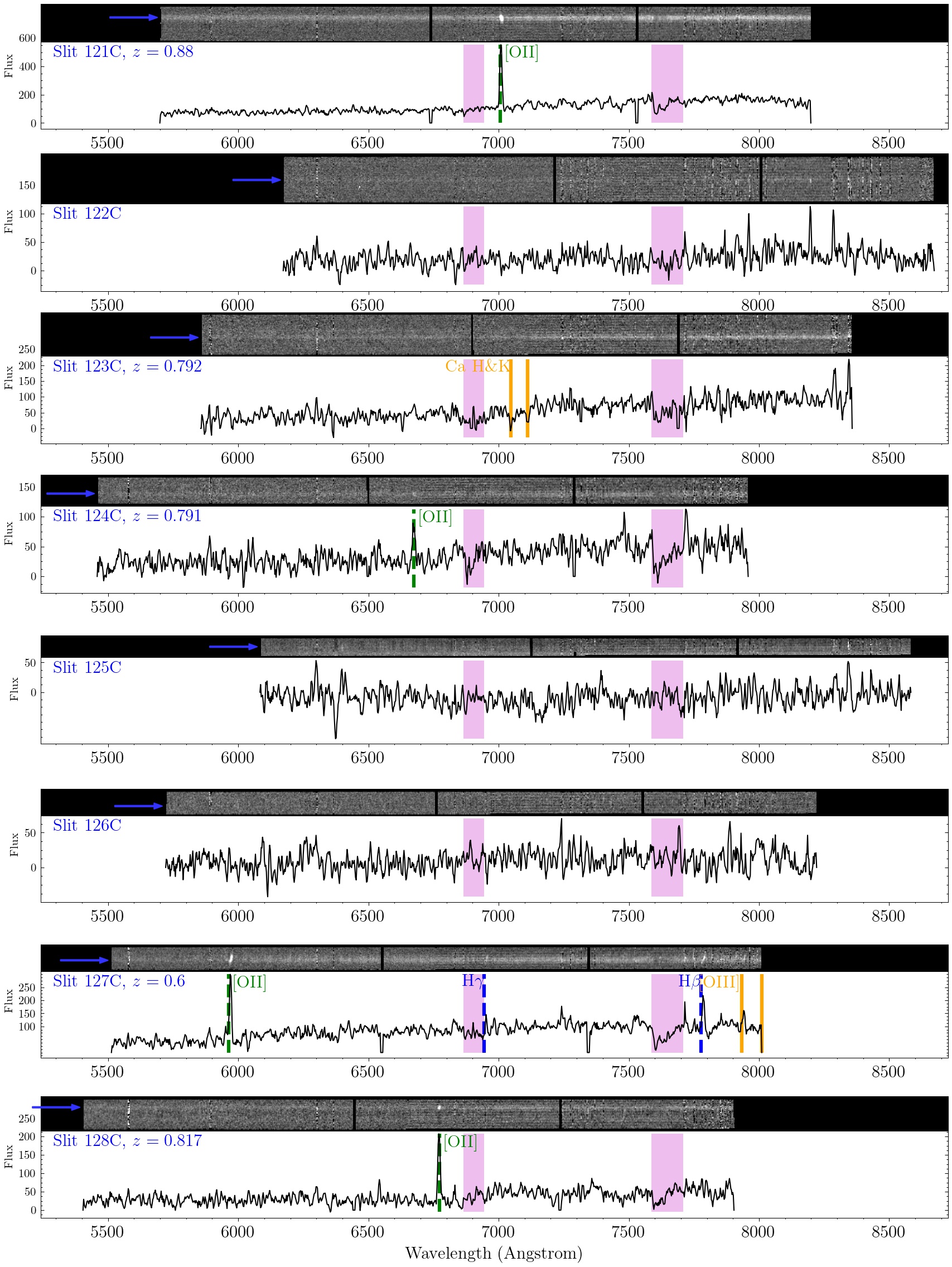
Figure 47: Galaxy Spectra of Slit #121C–128C.

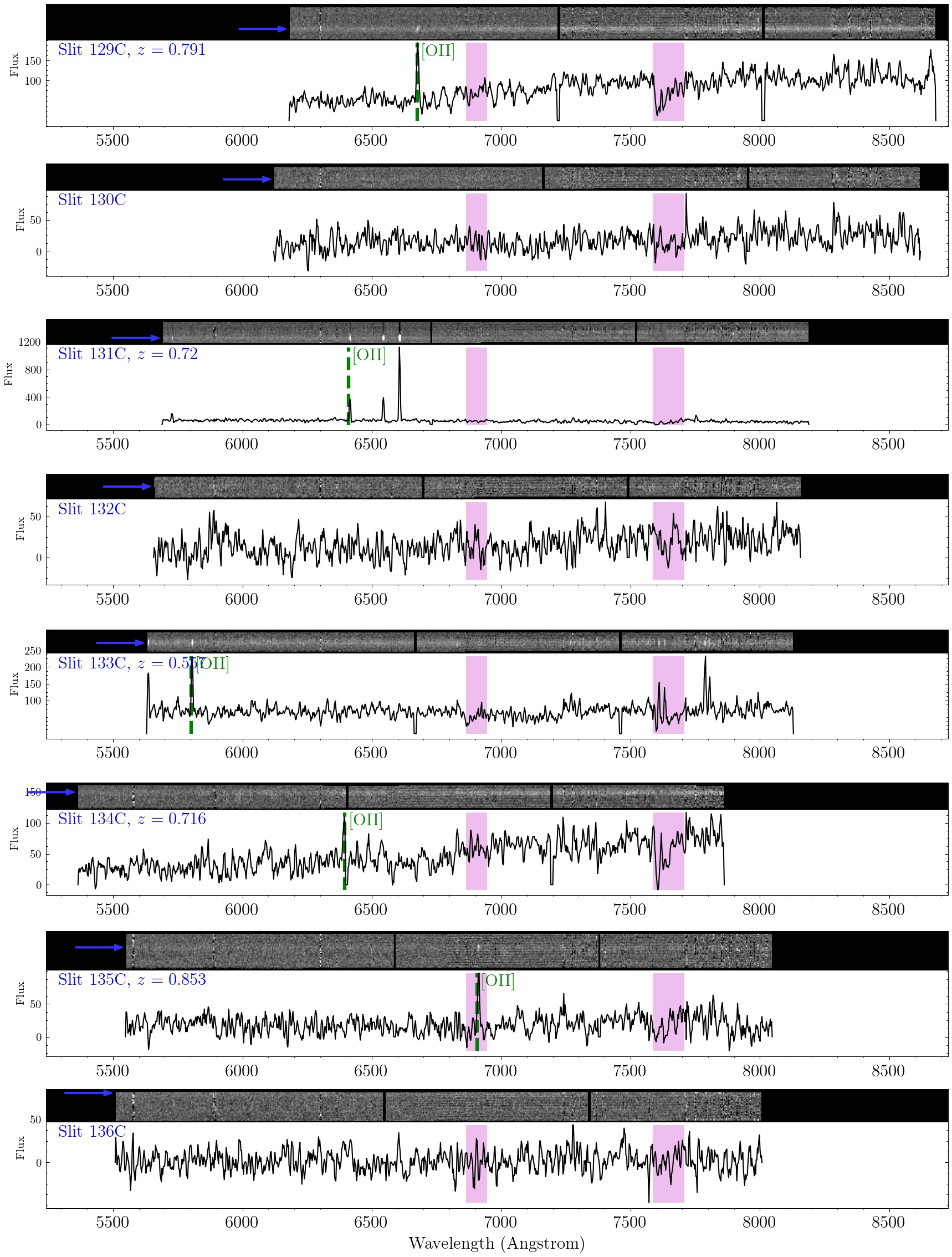
Figure 48: Galaxy Spectra of Slit #129C–136C.

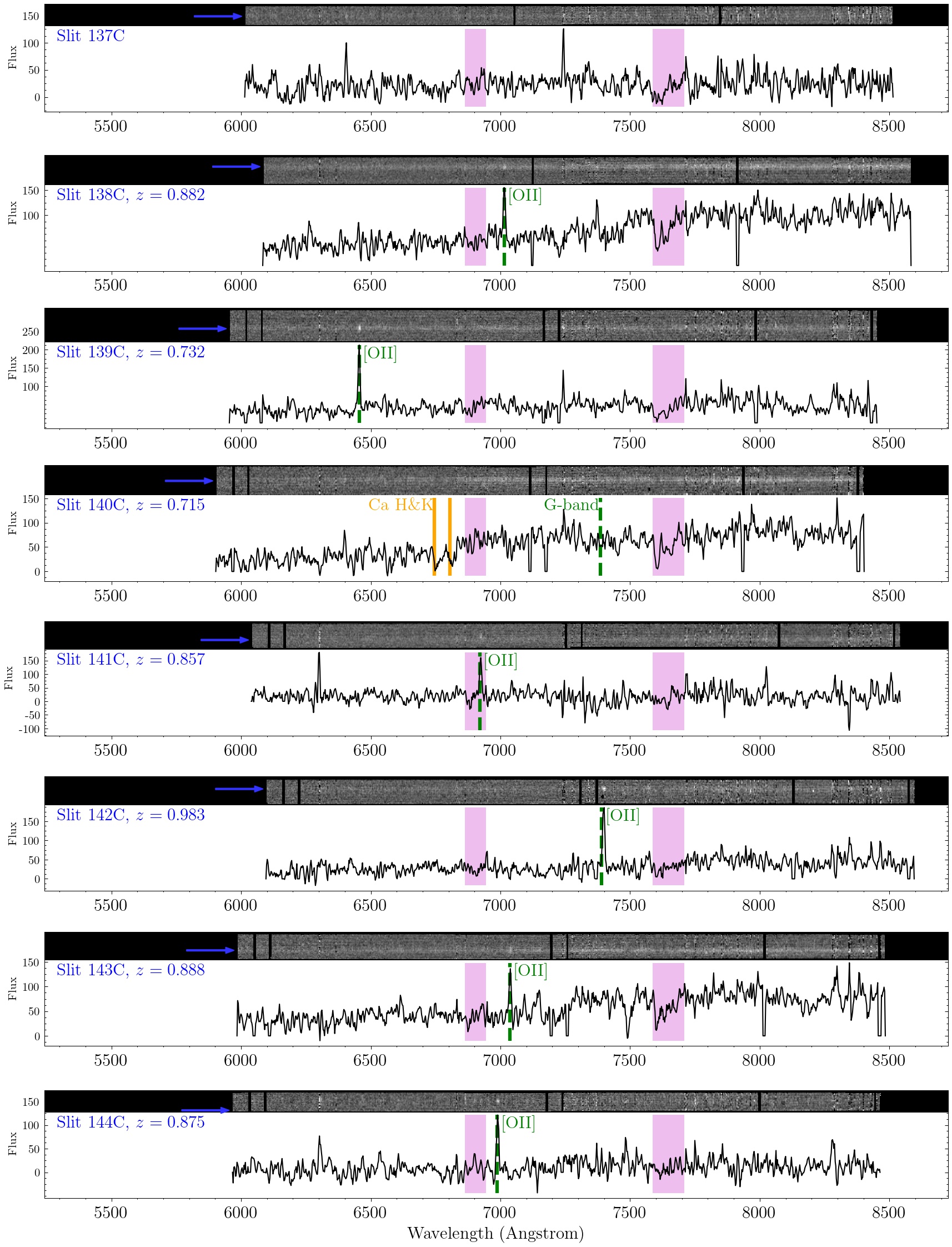
Figure 49: Galaxy Spectra of Slit #137C–144C.

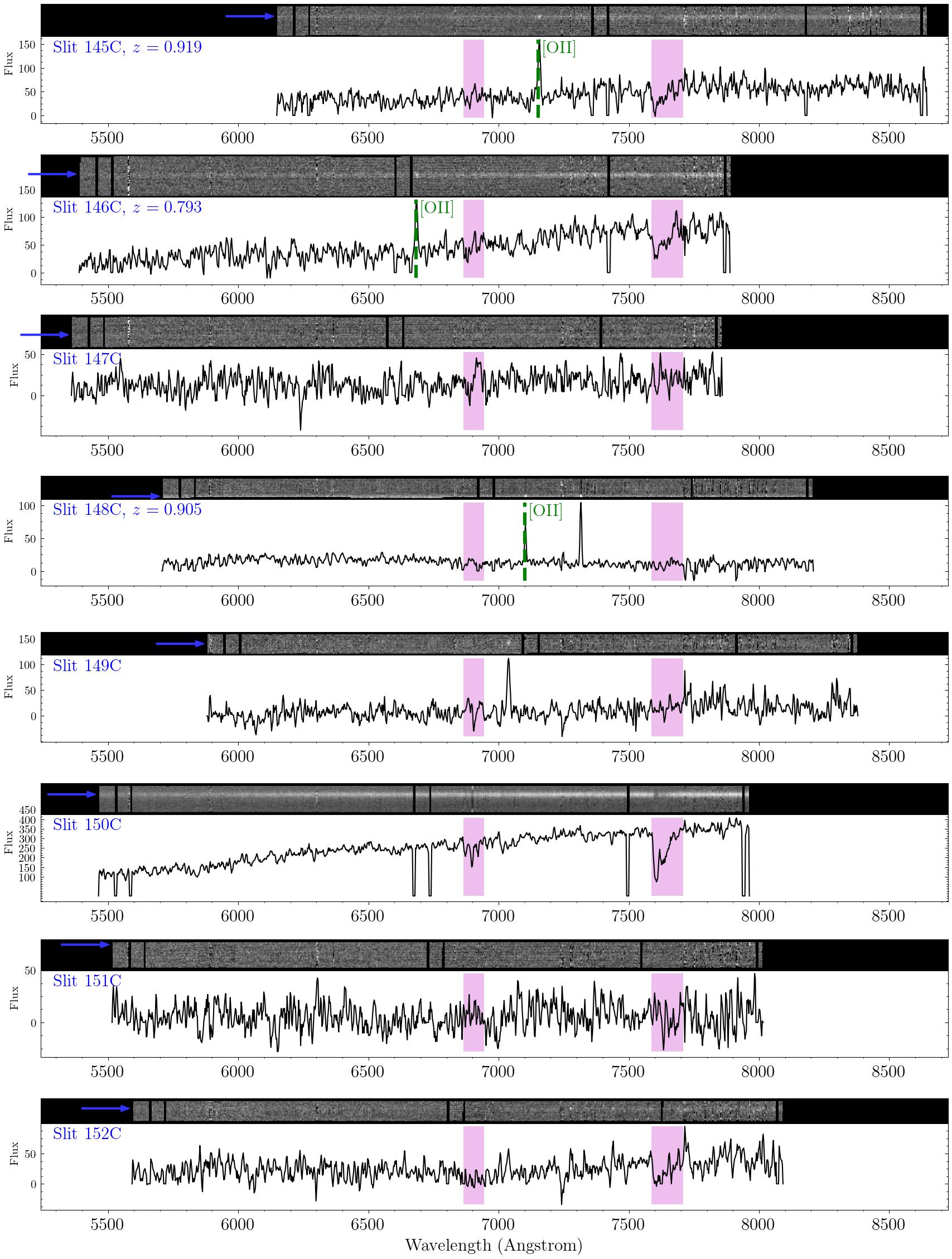
Figure 50: Galaxy Spectra of Slit #145C–152C.

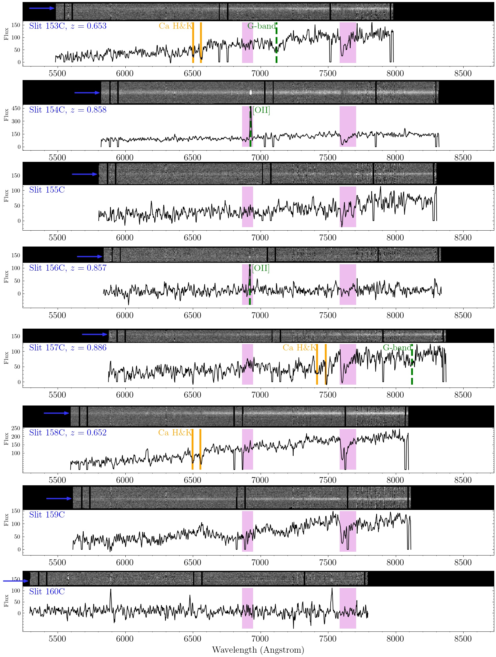
Figure 51: Galaxy Spectra of Slit #153C–160C.

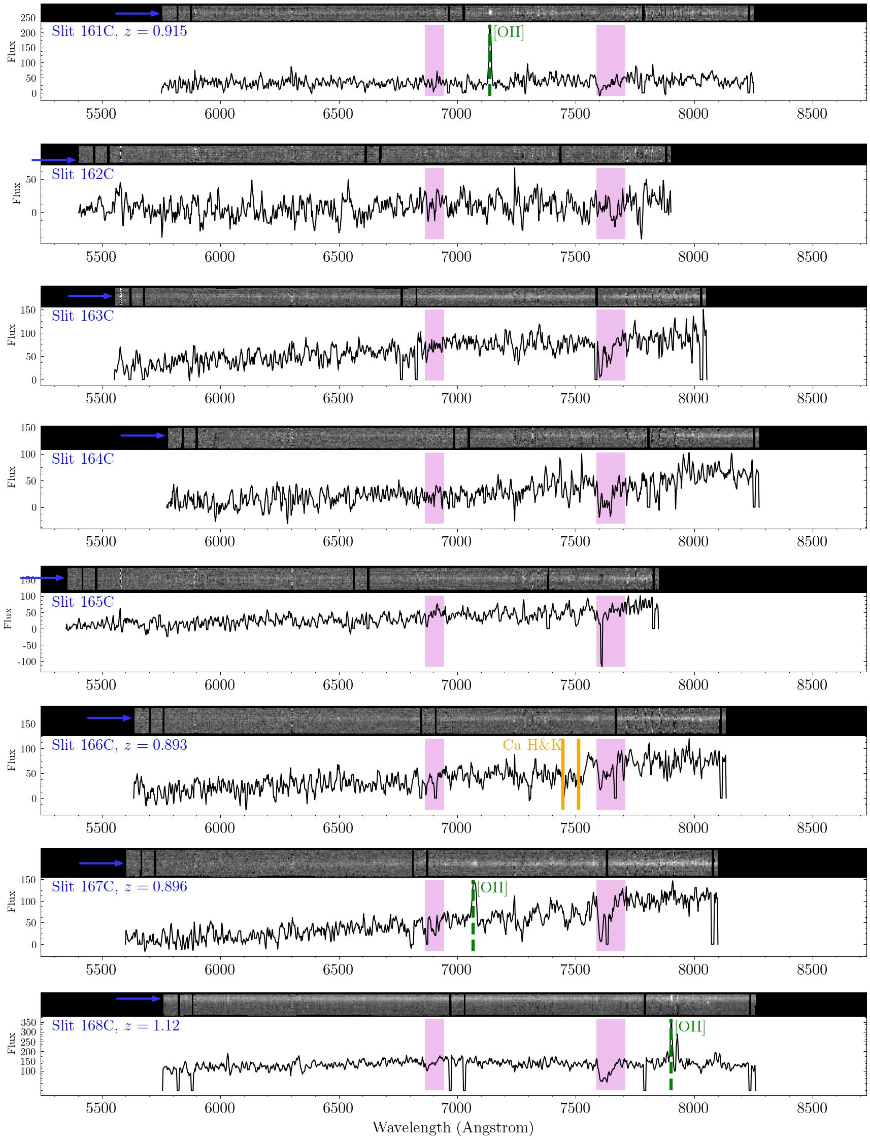
Figure 52: Galaxy Spectra of Slit #161C–168C.

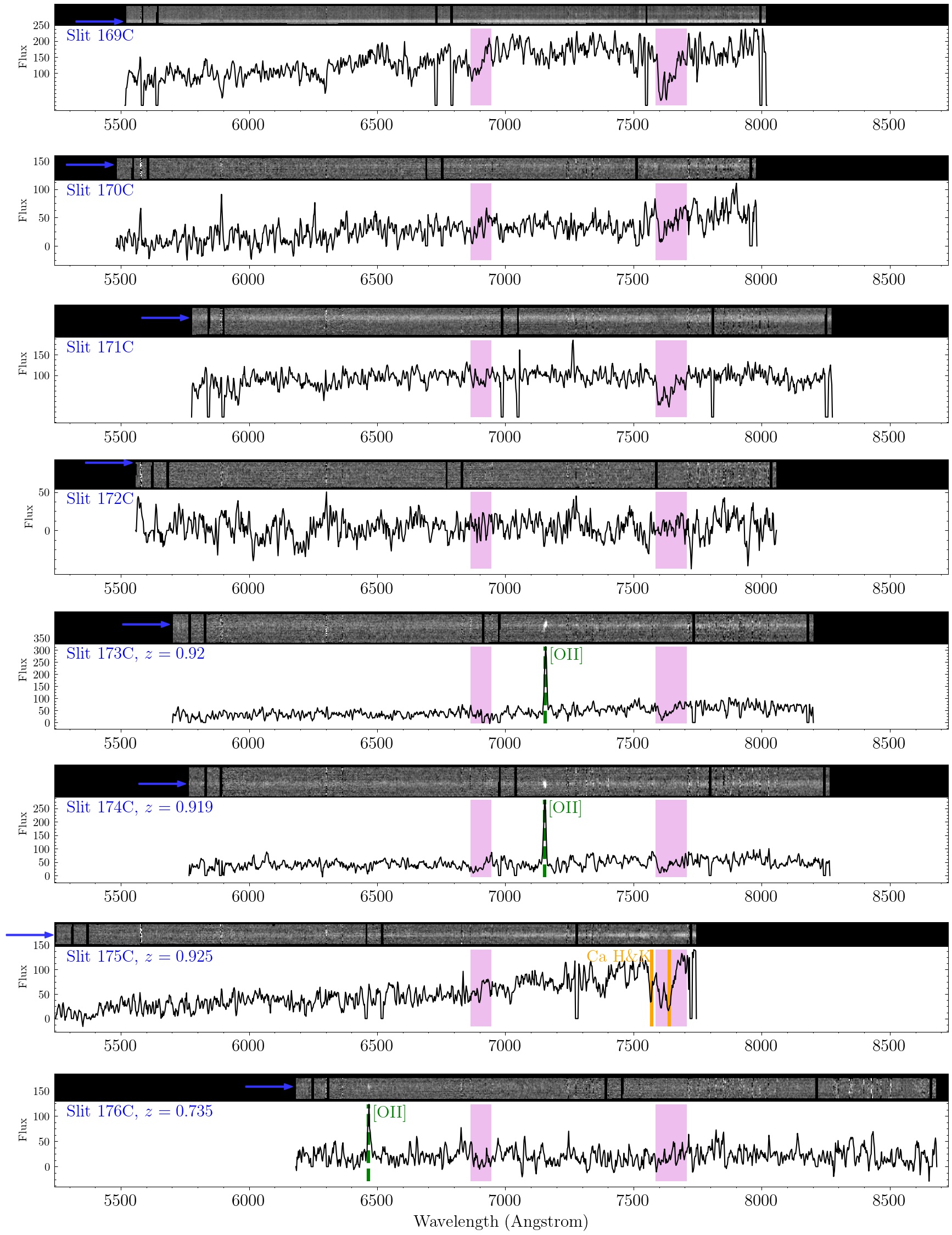
Figure 53: Galaxy Spectra of Slit #169C–176C.

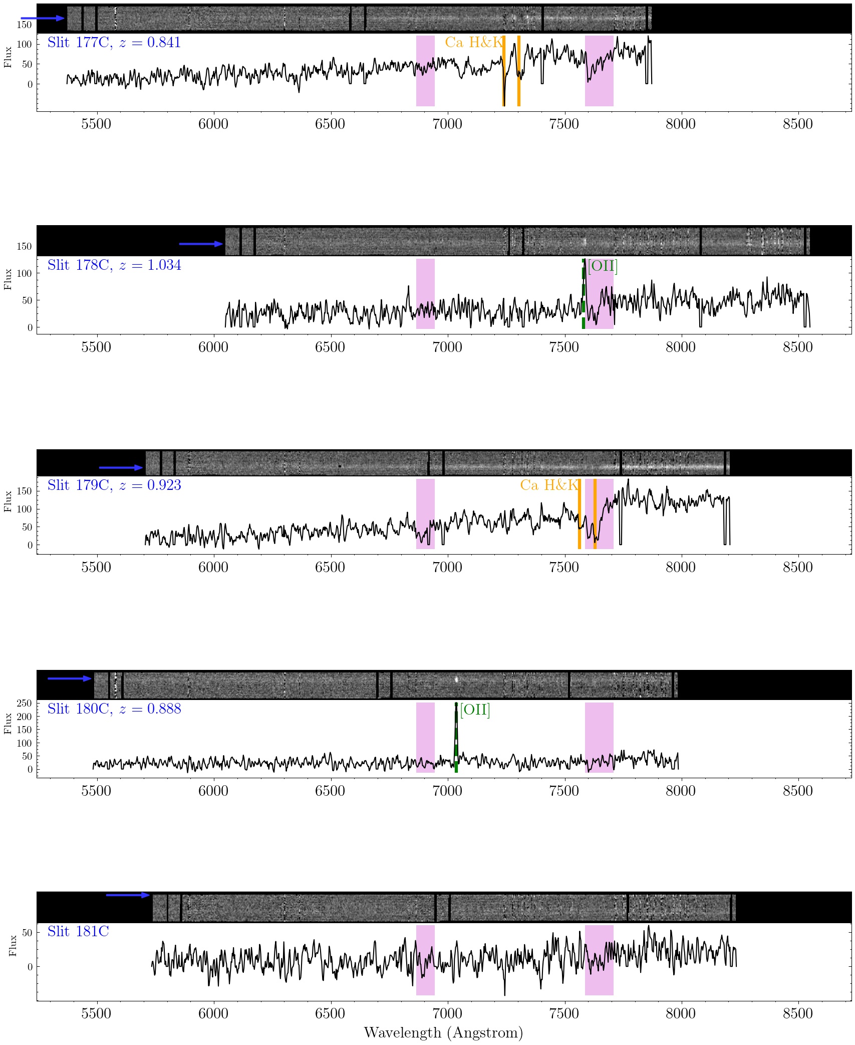
Figure 54: Galaxy Spectra of Slit #177C–181C.

References

- Aihara et al. (2018) Aihara, H., Arimoto, N., Armstrong, R., et al. 2018, PASJ, 70, 1, doi: 10.1093/pasj/psx066
- Allen et al. (2011) Allen, S. W., Evrard, A. E., & Mantz, A. B. 2011, Annual Review of A&A, 49, 409, doi: 10.1146/annurev-astro-081710-102514
- Astropy Collaboration et al. (2013) Astropy Collaboration, Robitaille, T. P., Tollerud, E. J., et al. 2013, A&A, 558, 1, doi: 10.1051/0004-6361/201322068
- Bleem et al. (2015) Bleem, L. E., Stalder, B., De Haan, T., et al. 2015, ApJ, Supplement Series, 216, doi: 10.1088/0067-0049/216/2/27
- Carnall et al. (2019) Carnall, A. C., Leja, J., Johnson, B. D., et al. 2019, ApJ, 873, 44, doi: 10.3847/1538-4357/ab04a2
- Carnall et al. (2018) Carnall, A. C., McLure, R. J., Dunlop, J. S., & Davé, R. 2018, MNRAS, 480, 4379, doi: 10.1093/mnras/sty2169
- Dey et al. (2019) Dey, A., Schlegel, D. J., Lang, D., et al. 2019, AJ, 157, 168, doi: 10.3847/1538-3881/ab089d
- Evrard et al. (2008) Evrard, A. E., Bialek, J., Busha, M., et al. 2008, ApJ, 672, 122, doi: 10.1086/521616
- Fabricant et al. (2019) Fabricant, D., Fata, R., Epps, H., et al. 2019, PASP, 131, 075004, doi: 10.1088/1538-3873/ab1d78
- Fadda et al. (1996) Fadda, D., Girardi, M., Iuricin, G., Mardirossian, F., & Mezzetti, M. 1996, ApJ, 473, 670, doi: 10.1086/178180
- Garrett (2021) Garrett, J. D. 2021, Zenodo, doi: 10.5281/zenodo.4106649
- Gavazzi et al. (2008) Gavazzi, R., Treu, T., Koopmans, L. V. E., et al. 2008, ApJ, 677, 1046, doi: 10.1086/529541
- Girardi et al. (1998) Girardi, M., Giuricin, G., Mardirossian, F., Mezzetti, M., & Boschin, W. 1998, ApJ, 505, 74, doi: 10.1086/306157
- Harris et al. (2020) Harris, C. R., Millman, K. J., van der Walt, S. J., et al. 2020, Computing in Science & Engineering, 9, 21, doi: 10.1038/s41586-020-2649-2
- Hasselfield et al. (2013) Hasselfield, M., Hilton, M., Marriage, T. A., et al. 2013, JCAP, 2013, 008, doi: 10.1088/1475-7516/2013/07/008
- Huang et al. (2018) Huang, S., Leauthaud, A., Murata, R., et al. 2018, PASJ, 70, 1, doi: 10.1093/pasj/psx126
- Hunter (2007) Hunter, J. D. 2007, Computing in Science & Engineering, 9, 90, doi: 10.1109/MCSE.2007.55
- Khullar et al. (2022) Khullar, G., Bayliss, M. B., Gladders, M. D., et al. 2022, ApJ, 934, 177, doi: 10.3847/1538-4357/ac7c0c
- Kravtsov & Borgani (2012) Kravtsov, A. V., & Borgani, S. 2012, Annual Review of A&A, 50, 353, doi: 10.1146/annurev-astro-081811-125502
- Lee & Komatsu (2010) Lee, J., & Komatsu, E. 2010, ApJ, 718, 60, doi: 10.1088/0004-637X/718/1/60
- Man et al. (2021) Man, A. W. S., Zabl, J., Brammer, G. B., et al. 2021, ApJ, 919, 20, doi: 10.3847/1538-4357/ac0ae3
- Mantz et al. (2010) Mantz, A., Allen, S. W., Rapetti, D., & Ebeling, H. 2010, MNRAS, 406, 1759, doi: 10.1111/j.1365-2966.2010.16992.x
- Masters & Capak (2011) Masters, D., & Capak, P. 2011, PASP, 123, 638, doi: 10.1086/660023
- Menci et al. (2008) Menci, N., Rosati, P., Gobat, R., et al. 2008, ApJ, 685, 863, doi: 10.1086/591016
- Mobasher et al. (2015) Mobasher, B., Dahlen, T., Ferguson, H. C., et al. 2015, ApJ, 808, doi: 10.1088/0004-637X/808/1/101
- Nishizawa et al. (2018) Nishizawa, A. J., Oguri, M., Oogi, T., et al. 2018, PASJ, 70, 1, doi: 10.1093/pasj/psx106
- Oguri (2014) Oguri, M. 2014, MNRAS, 444, 147, doi: 10.1093/mnras/stu1446
- Oguri et al. (2018) Oguri, M., Lin, Y.-T., Lin, S.-C., et al. 2018, PASJ, 70, S20, doi: 10.1093/pasj/psx042
- Perez & Granger (2007) Perez, F., & Granger, B. E. 2007, Computing in Science & Engineering, 9, 21, doi: 10.1109/MCSE.2007.53
- Reichardt et al. (2013) Reichardt, C. L., Stalder, B., Bleem, L. E., et al. 2013, ApJ, 763, 127, doi: 10.1088/0004-637X/763/2/127
- Rines et al. (2022) Rines, K. J., Sohn, J., Geller, M. J., & Diaferio, A. 2022, ApJ, 930, 156, doi: 10.3847/1538-4357/ac67a8
- Shah et al. (2020) Shah, E. A., Kartaltepe, J. S., Magagnoli, C. T., et al. 2020, ApJ, 904, 107, doi: 10.3847/1538-4357/abbf59
- Sifón et al. (2013) Sifón, C., Menanteau, F., Hasselfield, M., et al. 2013, ApJ, 772, 25, doi: 10.1088/0004-637X/772/1/25
- Sifón et al. (2016) Sifón, C., Battaglia, N., Hasselfield, M., et al. 2016, MNRAS, 461, 248, doi: 10.1093/mnras/stw1284
- Sunyaev & Zeldovich (1972) Sunyaev, R. A., & Zeldovich, Y. B. 1972, Comments on Astrophysics and Space Physics, 4, 173. https://ui.adsabs.harvard.edu/abs/1972CoASP...4..173S
- Tanaka et al. (2020) Tanaka, K., Tsuji, A., Akamatsu, H., et al. 2020, MNRAS, 491, 3411, doi: 10.1093/mnras/stz3188
- Tanaka (2015) Tanaka, M. 2015, ApJ, 801, 20, doi: 10.1088/0004-637X/801/1/20
- Tanaka et al. (2016) Tanaka, M., Wong, K. C., More, A., et al. 2016, ApJ, 826, L19, doi: 10.3847/2041-8205/826/2/L19
- Tanaka et al. (2018) Tanaka, M., Coupon, J., Hsieh, B.-C., et al. 2018, PASJ, 70, 1, doi: 10.1093/pasj/psx077
- Tu et al. (2009) Tu, H., Gavazzi, R., Limousin, M., et al. 2009, A&A, 501, 475, doi: 10.1051/0004-6361/200911963
- Virtanen et al. (2020) Virtanen, P., Gommers, R., Oliphant, T. E., et al. 2020, Nature Methods, 17, 261, doi: 10.1038/s41592-019-0686-2
- Worthey (1994) Worthey, G. 1994, ApJS, 95, 107, doi: 10.1086/192096