DiffiT: Diffusion Vision Transformers for Image Generation

Abstract

Diffusion models with their powerful expressivity and high sample quality have enabled many new applications and use-cases in various domains. For sample generation, these models rely on a denoising neural network that generates images by iterative denoising. Yet, the role of denoising network architecture is not well-studied with most efforts relying on convolutional residual U-Nets. In this paper, we study the effectiveness of vision transformers in diffusion-based generative learning. Specifically, we propose a new model, denoted as Diffusion Vision Transformers (DiffiT), which consists of a hybrid hierarchical architecture with a U-shaped encoder and decoder. We introduce a novel time-dependent self-attention module that allows attention layers to adapt their behavior at different stages of the denoising process in an efficient manner. We also introduce latent DiffiT which consists of transformer model with the proposed self-attention layers, for high-resolution image generation. Our results show that DiffiT is surprisingly effective in generating high-fidelity images, and it achieves state-of-the-art (SOTA) benchmarks on a variety of class-conditional and unconditional synthesis tasks. In the latent space, DiffiT achieves a new SOTA FID score of 1.73 on ImageNet-256 dataset. Repository: https://github.com/NVlabs/DiffiT.

1 Introduction

Diffusion models [64, 25, 66] have revolutionized the domain of generative learning, with successful frameworks in the front line such as DALL$\cdot$E 3 [54], Imagen [26], Stable diffusion  [56, 55], and eDiff-I [6]. They have enabled generating diverse complex scenes in high fidelity which were once considered out of reach for prior models. Specifically, synthesis in diffusion models is formulated as an iterative process in which random image-shaped Gaussian noise is denoised gradually towards realistic samples [64, 25, 66]. The core building block in this process is a denoising autoencoder network that takes a noisy image and predicts the denoising direction, equivalent to the score function [71, 30]. This network, which is shared across different time steps of the denoising process, is often a variant of U-Net [57, 25] that consists of convolutional residual blocks as well as self-attention layers in several resolutions of the network. Although the self-attention layers have shown to be important for capturing long-range spatial dependencies, yet there exists a lack of standard design patterns on how to incorporate them. In fact, most denoising networks often leverage self-attention layers only in their low-resolution feature maps [14] to avoid their expensive computational complexity. Recently, several works [6, 42, 11] have observed that diffusion models exhibit a unique temporal dynamic during generation. At the beginning of the denoising process, when the image contains strong Gaussian noise, the high-frequency content of the image is completely perturbed, and the denoising network primarily focuses on predicting the low-frequency content. However, towards the end of denoising, in which most of the image structure is generated, the network tends to focus on predicting high-frequency details. The time dependency of the denoising network is often implemented via simple temporal positional embeddings that are fed to different residual blocks via arithmetic operations such as spatial addition. In fact, the convolutional filters in the denoising network are not time-dependent and the time embedding only applies a channel-wise shift and scaling. Hence, such a simple mechanism may not be able to optimally capture the time dependency of the network during the entire denoising process.

In this work, we aim to address the issue of lacking fine-grained control over capturing the time-dependent component in self-attention modules for denoising diffusion models. We introduce a novel Vision Transformer-based model for image generation, called DiffiT (pronounced di-feet) which achieves state-of-the-art performance in terms of FID score of image generation on CIFAR10 [43] and FFHQ-64 [32] (image space) as well as ImageNet-256 [13] and ImageNet-512 [13] (latent space) datasets. Specifically, DiffiT proposes a new paradigm in which temporal dependency is only integrated into the self-attention layers where the key, query, and value weights are adapted per time step. This allows the denoising model to dynamically change its attention mechanism for different denoising stages. In an effort to unify the architecture design patterns, we also propose a hierarchical transformer-based architecture for latent space synthesis tasks.

The following summarizes our contributions in this work:

• We introduce a novel time-dependent self-attention module that is specifically tailored to capture both short- and long-range spatial dependencies. Our proposed time-dependent self-attention dynamically adapts its behavior over sampling time steps.

• We propose a novel transformer-based architecture, denoted as DiffiT, which unifies the design patterns of denoising networks.

• We show that DiffiT can achieve state-of-the-art performance on a variety of datasets for both image and latent space generation tasks.

2 Related Work

Transformers in Generative Modeling

Transformer-based models have achieved competitive performance in different generative learning models in the visual domain [10, 79, 16, 80, 27, 15]. A number of transformer-based architectures have emerged for GANs [46, 75, 82, 45]. TransGAN [31] proposed to use a pure transformer-based generator and discriminator architecture for pixel-wise image generation. Gansformer [29] introduced a bipartite transformer that encourages the similarity between latent and image features. Styleformer [51] uses Linformers [72] to scale the synthesis to higher resolution images. Recently, a number of efforts [48, 7, 52, 21] have leveraged Transformer-based architectures for diffusion models and achieved competitive performance. In particular, Diffusion Transformer (DiT) [52] proposed a latent diffusion model in which the regular U-Net backbone is replaced with a Transformer. In DiT, the conditioning on input noise is done by using Adaptive LayerNorm (AdaLN) [53] blocks. Using the DiT architecture, Masked Diffusion Transformer (MDT) [21] introduced a masked latent modeling approach to effectively capture contextual information. In comparison to DiT, although MDT achieves faster learning speed and better FID scores on ImageNet-256 dataset [13], it has a more complex training pipeline. Unlike DiT and MDT, the proposed DiffiT does not use shift and scale, as in AdaLN formulation, for conditioning. Instread, DiffiT proposes a time-dependent self-attention (i.e. TMSA) to jointly learn the spatial and temporal dependencies. In addition, DiffiT proposes both image and latent space models for different image generation tasks with different resolutions with SOTA performance.

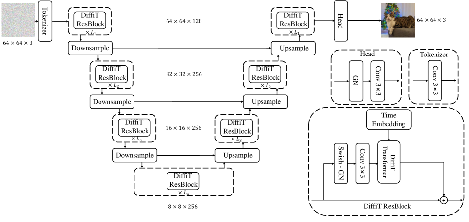
Figure 2: Overview of the image-space DiffiT model. Downsample and Upsample denote convolutional downsampling and upsampling layers, respectively. Please see the supplementary materials for more information regarding the DiffiT architecture.

Diffusion Image Generation

Diffusion models [64, 25, 66] have driven significant advances in various domains, such as text-to-image generation [54, 59, 6], natural language processing [47], text-to-speech synthesis [41], 3D point cloud generation [78, 77, 84], time series modeling [67], molecular conformal generation [74], and machine learning security [50]. These models synthesize samples via an iterative denoising process and thus are also known in the community as noise-conditioned score networks. Since its initial success on small-scale datasets like CIFAR-10 [25], diffusion models have been gaining popularity compared to other existing families of generative models. Compared with variational autoencoders [40], diffusion models divide the synthesis procedure into small parts that are easier to optimize, and have better coverage of the latent space [2, 63, 69]; compared with generative adversarial networks [23], diffusion models have better training stability and are much easier to invert [65, 20]. Diffusion models are also well-suited for image restoration, editing and re-synthesis tasks with minimal modifications to the existing architecture [49, 58, 20, 37, 3, 4, 12, 35, 36, 70], making it well-suited for various downstream applications.

3 Methodology

3.1 Diffusion Model

Diffusion models [64, 25, 66] are a family of generative models that synthesize samples via an iterative denoising process. Given a data distribution as $q_{0}({\mathbf{z}}_{0})$, a family of random variables ${\mathbf{z}}_{t}$ for $t\in[0,T]$ are defined by injecting Gaussian noise to ${\mathbf{z}}_{0}$, i.e., $q_{t}({\mathbf{z}}_{t})=\int q({\mathbf{z}}_{t}|{\mathbf{z}}_{0})q_{0}({\mathbf{z}}_{0})\mathrm{d}{\mathbf{z}}_{0}$, where $q({\mathbf{z}}_{t}|{\mathbf{z}}_{0})={\mathcal{N}}({\mathbf{z}}_{0},\sigma_{t}^{2}{\bm{I}})$ is a Gaussian distribution. Typically, $\sigma_{t}$ is chosen as a non-decreasing sequence such that $\sigma_{0}=0$ and $\sigma_{T}$ being much larger than the data variance. This is called the “Variance-Exploding” noising schedule in the literature [66]; for simplicity, we use these notations throughout the paper, but we note that it can be equivalently converted to other commonly used schedules (such as “Variance-Preserving” [25]) by simply rescaling the data with a scaling term, dependent on $t$ [65, 34].

The distributions of these random variables are the marginal distributions of forward diffusion processes (Markovian or not [65]) that gradually reduces the “signal-to-noise” ratio between the data and noise. As a generative model, diffusion models are trained to approximate the reverse diffusion process, that is, to transform from the initial noisy distribution (that is approximately Gaussian) to a distribution that is close to the data one.

Training

Despite being derived from different perspectives, diffusion models can generally be written as learning the following denoising autoencoder objective [71]

$${\mathbb{E}}_{q_{0}({\mathbf{z}}_{0}),t\sim p(t),\epsilon\sim{\mathcal{N}}(0,{\bm{I}})}[\lambda(t){\lVert{\epsilon-\epsilon_{\theta}({\mathbf{z}}_{0}+\sigma_{t}\epsilon,t)}\rVert}_{2}^{2}].$$ (1)

Intuitively, given a noisy sample from $q({\mathbf{z}}_{t})$ (generated via ${\mathbf{z}}_{t}:={\mathbf{z}}_{0}+\sigma_{t}\epsilon$), a neural network $\epsilon_{\theta}$ is trained to predict the amount of noise added (i.e., $\epsilon$). Equivalently, the neural network can also be trained to predict ${\mathbf{z}}_{0}$ instead [25, 60]. The above objective is also known as denoising score matching [71], where the goal is to try to fit the data score (i.e., $\nabla_{{\mathbf{z}}_{t}}\log q({\mathbf{z}}_{t})$) with a neural network, also known as the score network $s_{\theta}({\mathbf{z}}_{t},t)$. The score network can be related to $\epsilon_{\theta}$ via the relationship $s_{\theta}({\mathbf{z}}_{t},t):=-\epsilon_{\theta}({\mathbf{z}}_{t},t)/\sigma_{t}$.

Sampling

Samples from the diffusion model can be simulated by the following family of stochastic differential equations that solve from $t=T$ to $t=0$ [24, 34, 81, 17]:

$$\mathrm{d}{\mathbf{z}}=-(\dot{\sigma}_{t}+\beta_{t})\sigma_{t}s_{\theta}({\mathbf{z}},t)\mathrm{d}t+\sqrt{2\beta_{t}}\sigma_{t}\mathrm{d}\omega_{t},$$ (2)

where $\omega_{t}$ is the reverse standard Wiener process, and $\beta_{t}$ is a function that describes the amount of stochastic noise during the sampling process. If $\beta_{t}=0$ for all $t$, then the process becomes a probabilistic ordinary differential equation [1] (ODE), and can be solved by ODE integrators such as denoising diffusion implicit models (DDIM [65]). Otherwise, solvers for stochastic differential equations (SDE) can be used, including the one for the original denoising diffusion probabilistic models (DDPM [25]). Typically, ODE solvers can converge to high-quality samples in fewer steps and SDE solvers are more robust to inaccurate score models [34].

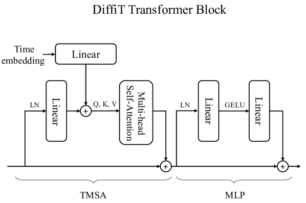
Figure 3: The DiffiT Transformer block applies linear projection to spatial and time-embedding tokens before combining them together to form query, key, and value vectors for each token. These vectors are then used to compute multi-head self-attention activations, followed by two linear layers.

3.2 DiffiT Model

Time-dependent Self-Attention

At every layer, our transformer block receives $\{\mathbf{x_{s}}\}$, a set of tokens arranged spatially on a 2D grid in its input. It also receives $\mathbf{x_{t}}$, a time token representing the time step. Similar to  Ho et al. [25], we obtain the time token by feeding positional time embeddings to a small MLP with swish activation [19]. This time token is passed to all layers in our denoising network. We introduce our time-dependent multi-head self-attention, which captures both long-range spatial and temporal dependencies by projecting feature and time token embeddings in a shared space. Specifically, time-dependent queries $\mathbf{q}$, keys $\mathbf{k}$ and values $\mathbf{v}$ in the shared space are computed by a linear projection of spatial and time embeddings $\mathbf{x_{s}}$ and $\mathbf{x_{t}}$ via

$$\mathbf{q_{s}} =\mathbf{x_{s}}\mathbf{W}_{qs}+\mathbf{x_{t}}\mathbf{W}_{qt},$$ (3)

$$\mathbf{k_{s}} =\mathbf{x_{s}}\mathbf{W}_{ks}+\mathbf{x_{t}}\mathbf{W}_{kt},$$ (4)

$$\mathbf{v_{s}} =\mathbf{x_{s}}\mathbf{W}_{vs}+\mathbf{x_{t}}\mathbf{W}_{vt},$$ (5)

where $\mathbf{W}_{qs}$, $\mathbf{W}_{qt}$, $\mathbf{W}_{ks}$, $\mathbf{W}_{kt}$, $\mathbf{W}_{vs}$, $\mathbf{W}_{vt}$ denote spatial and temporal linear projection weights for their corresponding queries, keys, and values respectively.

We note that the operations listed in Eq. 3 to 5 are equivalent to a linear projection of each spatial token, concatenated with the time token. As a result, key, query, and value are all linear functions of both time and spatial tokens and they can adaptively modify the behavior of attention for different time steps. We define $\mathbf{Q}:=\{\mathbf{q_{s}}\}$, $\mathbf{K}:=\{\mathbf{k_{s}}\}$, and $\mathbf{V}:=\{\mathbf{v_{s}}\}$ which are stacked form of query, key, and values in rows of a matrix. The self-attention is then computed as follows

$$\operatorname{Attention}(\mathbf{Q},\mathbf{K},\mathbf{V})=\operatorname{Softmax}\left(\frac{\mathbf{Q}\mathbf{K}^{\top}}{\sqrt{d}}+\mathbf{B}\right)\mathbf{V}.$$ (6)

In which, $d$ is a scaling factor for keys $\mathbf{K}$, and B corresponds to a relative position bias [62]. For computing the attention, the relative position bias allows for the encoding of information across each attention head. Note that although the relative position bias is implicitly affected by the input time embedding, directly integrating it with this component may result in sub-optimal performance as it needs to capture both spatial and temporal information. Please see Sec. 5.4 for more analysis.

DiffiT Block

The DiffiT transformer block (see Fig. 3) is a core building block of the proposed architecture and is defined as

$$\bf{\hat{x}_{s}} =\text{TMSA}\left({\text{LN}\left(\bf{x_{s}}\right)},\bf{x_{t}}\right)+\bf{x_{s}},$$ (7)

$$\bf{x_{s}} =\text{MLP}\left({\text{LN}\left(\bf{\hat{x}_{s}}\right)}\right)+\bf{\hat{x}_{s}},$$ (8)

where TMSA denotes time-dependent multi-head self-attention, as described in the above, $\bf{x_{t}}$ is the time-embedding token, $\bf{x_{s}}$ is a spatial token, and LN and MLP denote Layer Norm [5] and multi-layer perceptron (MLP) respectively.

3.2.1 Image Space

DiffiT Architecture

DiffiT uses a symmetrical U-Shaped encoder-decoder architecture in which the contracting and expanding paths are connected to each other via skip connections at every resolution. Specifically, each resolution of the encoder or decoder paths consists of $L$ consecutive DiffiT blocks, containing our proposed time-dependent self-attention modules. In the beginning of each path, for both the encoder and decoder, a convolutional layer is employed to match the number of feature maps. In addition, a convolutional upsampling or downsampling layer is also used for transitioning between each resolution. We speculate that the use of these convolutional layers embeds inductive image bias that can further improve the performance. In the remainder of this section, we discuss the DiffiT Transformer block and our proposed time-dependent self-attention mechanism. We use our proposed Transformer block as the residual cells when constructing the U-shaped denoising architecture.

DiffiT ResBlock

We define our final residual cell by combining our proposed DiffiT Transformer block with an additional convolutional layer in the form:

$$\bf{\hat{x}_{s}} =\text{Conv}_{3\times 3}\left(\text{Swish}\left(\text{GN}\left(\bf{x_{s}}\right)\right)\right),$$ (9)

$$\bf{x_{s}} =\text{DiffiT-Block}\left(\bf{\hat{x}_{s}},\bf{x_{t}}\right)+\bf{x_{s}},$$ (10)

where GN denotes the group normalization operation [73] and DiffiT-Transformer is defined in Eq. 7 and Eq. 8 (shown in Fig. 3). Our residual cell for image space diffusion models is a hybrid cell combining both a convolutional layer and our Transformer block.

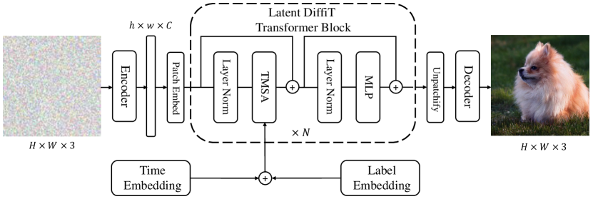
Figure 4: Overview of the latent DiffiT framework.

Figure 5: Visualization of uncurated generated images for FFHQ-64 dataset. Best viewed in color.

3.2.2 Latent Space

Recently, latent diffusion models have been shown effective in generating high-quality large-resolution images [69, 56]. In Fig. 4, we show the architecture of latent DiffiT model. We first encode the images using a pre-trained variational auto-encoder network [56]. The feature maps are then converted into non-overlapping patches and projected into a new embedding space. Similar to the DiT model [52], we use a vision transformer, without upsampling or downsampling layers, as the denoising network in the latent space. In addition, we also utilize a three-channel classifier-free guidance to improve the quality of generated samples. The final layer of the architecture is a simple linear layer to decode the output.

4 Results

4.1 Image Space

We have trained the proposed DiffiT model on CIFAR-10, FFHQ-64 datasets respectively. In Table. 1, we compare the performance of our model against a variety of different generative models including other score-based diffusion models as well as GANs, and VAEs. DiffiT achieves a state-of-the-art image generation FID score of 1.95 on the CIFAR-10 dataset, outperforming state-of-the-art diffusion models such as EDM [34] and LSGM [69]. In comparison to two recent ViT-based diffusion models, our proposed DiffiT significantly outperforms U-ViT [7] and GenViT [76] models in terms of FID score in CIFAR-10 dataset. Additionally, DiffiT significantly outperforms EDM [34] and DDPM++ [66] models, both on VP and VE training configurations, in terms of FID score. In Fig. 5, we illustrate the generated images on FFHQ-64 dataset. Please see supplementary materials for CIFAR-10 generated images.

Table 1: FID performance comparison against various generative approaches on the CIFAR10, FFHQ-64 datasets. VP and VE denote Variance Preserving and Variance Exploding respectively. DiffiT outperforms competing approaches, sometimes by large margins.

Method	Class	Space Type	CIFAR-10	FFHQ
			32$\times$32	64$\times$64
NVAE [68]	VAE	-	23.50	-
GenViT [76]	Diffusion	Image	20.20	-
AutoGAN [22]	GAN	-	12.40	-
TransGAN [31]	GAN	-	9.26	-
INDM [38]	Diffusion	Latent	3.09	-
DDPM++ (VE) [66]	Diffusion	Image	3.77	25.95
U-ViT [7]	Diffusion	Image	3.11	-
DDPM++ (VP) [66]	Diffusion	Image	3.01	3.39
StyleGAN2 w/ ADA [33]	GAN	-	2.92	-
LSGM [69]	Diffusion	Latent	2.01	-
EDM (VE) [34]	Diffusion	Image	2.01	2.53
EDM (VP) [34]	Diffusion	Image	1.99	2.39
DiffiT (Ours)	Diffusion	Image	1.95	2.22

4.2 Latent Space

We have also trained the latent DiffiT model on ImageNet-512 and ImageNet-256 dataset respectively. In Table. 2, we present a comparison against other approaches using various image quality metrics. For this comparison, we select the best performance metrics from each model which may include techniques such classifier-free guidance. In ImageNet-256 dataset, the latent DiffiT model outperforms competing approaches, such as MDT-G [21], DiT-XL/2-G [52] and StyleGAN-XL [61], in terms of FID score and sets a new SOTA FID score of 1.73. In terms of other metrics such as IS and sFID, the latent DiffiT model shows a competitive performance, hence indicating the effectiveness of the proposed time-dependant self-attention. In ImageNet-512 dataset, the latent DiffiT model significantly outperforms DiT-XL/2-G in terms of both FID and Inception Score (IS). Although StyleGAN-XL [61] shows better performance in terms of FID and IS, GAN-based models are known to suffer from issues such as low diversity that are not captured by the FID score. These issues are reflected in sub-optimal performance of StyleGAN-XL in terms of both Precision and Recall. In addition, in Fig. 6, we show a visualization of uncurated images that are generated on ImageNet-256 and ImageNet-512 dataset. We observe that latent DiffiT model is capable of generating diverse high quality images across different classes.

Model	Class	ImageNet-256				ImageNet-512
		FID $\downarrow$	IS $\uparrow$	Precision $\uparrow$	Recall $\uparrow$		FID $\downarrow$	IS $\uparrow$	Precision $\uparrow$	Recall $\uparrow$
LDM-4 [56]	Diffusion	10.56	103.49	0.71	0.62		-	-	-	-
BigGAN-Deep [8]	GAN	6.95	171.40	0.87	0.28		8.43	177.90	0.88	0.29
MaskGIT [9]	Masked Modeling	4.02	355.60	0.83	0.44		4.46	342.00	0.83	0.50
RQ-Transformer [44]	Autoregressive	3.80	323.70	-	-		-	-	-	-
ADM-G-U [14]	Diffusion	3.94	215.84	0.83	0.53		3.85	221.72	0.84	0.53
LDM-4-G [56]	Diffusion	3.60	247.67	0.87	0.48		-	-	-	-
Simple Diffusion [28]	Diffusion	2.77	211.80	-	-		3.54	205.30	-	-
DiT-XL/2-G [52]	Diffusion	2.27	278.24	0.83	0.57		3.04	240.82	0.84	0.54
StyleGAN-XL [61]	GAN	2.30	265.12	0.78	0.53		2.41	267.75	0.77	0.52
MDT-G [21]	Diffusion	1.79	283.01	0.81	0.61		-	-	-	-
DiffiT	Diffusion	1.73	276.49	0.80	0.62		2.67	252.12	0.83	0.55

Table 2: Comparison of image generation performance against state-of-the-art models on ImageNet-256 and ImageNet-512 dataset. The latent DiffiT model achieves SOTA performance in terms of FID score on ImageNet-256 dataset.

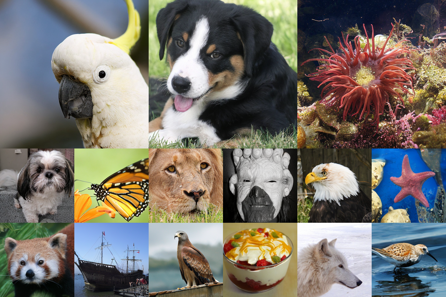
Figure 6: Visualization of uncurated generated images on ImageNet-256 and ImageNet-512 datasets by latent DiffiT model.

5 Ablation

In this section, we provide additional ablation studies to provide insights into DiffiT. We address four main questions: (1) What strikes the right balance between time and feature token dimensions ? (2) How do different components of DiffiT contribute to the final generative performance, (3) What is the optimal way of introducing time dependency in our Transformer block? and (4) How does our time-dependent attention behave as a function of time?

5.1 Time and Feature Token Dimensions

We conduct experiments to study the effect of the size of time and feature token dimensions on the overall performance. As shown below, we observe degradation of performance when the token dimension is increased from 256 to 512. Furthermore, decreasing the time embedding dimension from 512 to 256 impacts the performance negatively.

Time Dimension	Dimension	CIFAR10	FFHQ64
512	512	1.99	2.27
256	256	2.13	2.41
512	512	1.95	2.22

Table 3: Ablation study on the effectiveness of time and feature dimensions.

5.2 Effect of Architecture Design

As presented in Table 4, we study the effect of various components of both encoder and decoder in the architecture design on the image generation performance in terms of FID score on CIFAR-10. For these experiments, the projected temporal component is adaptively scaled and simply added to the spatial component in each stage. We start from the original ViT [18] base model with 12 layers and employ it as the encoder (config A). For the decoder, we use the Multi-Level Feature Aggregation variant of SETR [83] (SETR-MLA) to generate images in the input resolution. Our experiments show this architecture is sub-optimal as it yields a final FID score of 5.34. We hypothesize this could be due to the isotropic architecture of ViT which does not allow learning representations at multiple scales.

Config	Encoder	Decoder	FID Score
A	ViT [18]	SETR-MLA [83]	5.34
B	+ Multi-Resolution	SETR-MLA [83]	4.64
C	Multi-Resolution	+ Multi-Resolution	3.71
D	+ DiffiT Encoder	Multi-Resolution	2.27
E	+ DiffiT Encoder	+ DiffiT Decoder	1.95

Table 4: Ablation study on the effectiveness of encoder and decoder architecture.

We then extend the encoder ViT into 4 different multi-resolution stages with a convolutional layer in between each stage for downsampling (config B). We denote this setup as Multi-Resolution and observe that these changes and learning multi-scale feature representations in the encoder substantially improve the FID score to 4.64.

Model	TMSA	FID Score
DDPM++(VE) [66]	No	3.77
DDPM++(VE) [66]	Yes	3.49
DDPM++(VP) [66]	No	3.01
DDPM++(VP) [66]	Yes	2.76

Table 5: Impact of TMSA as a standalone module in other denoising networks.

In addition, instead of SETR-MLA [83] decoder, we construct a symmetric U-like architecture by using the same Multi-Resolution setup except for using convolutional layer between stage for upsampling (config C). These changes further improve the FID score to 3.71. Furthermore, we first add the DiffiT Transformer blocks and construct a DiffiT Encoder and observe that FID scores substantially improve to 2.27 (config D). As a result, this validates the effectiveness of the proposed TMSA in which the self-attention models both spatial and temporal dependencies. Using the DiffiT decoder further improves the FID score to 1.95 (config E), hence demonstrating the importance of DiffiT Transformer blocks for decoding.

5.3 Time-Dependent Self-Attention

We evaluate the effectiveness of our proposed TMSA layers in a generic denoising network. Specifically, using the DDPM++ [66] model, we replace the original self-attention layers with TMSA layers for both VE and VP settings for image generation on the CIFAR10 dataset. Note that we did not change the original hyper-parameters for this study. As shown in Table 5 employing TMSA decreases the FID scores by 0.28 and 0.25 for VE and VP settings respectively. These results demonstrate the effectiveness of the proposed TMSA to dynamically adapt to different sampling steps and capture temporal information.

Config	Component	FID Score
F	Relative Position Bias	3.97
G	MLP	3.81
H	TMSA	1.95

Table 6: The impact of TMSA design choices on FID score.

5.4 Impact of Self-Attention Components

In Table 6, we study different design choices for introducing time-dependency in self-attention layers. In the first baseline, we remove the temporal component from our proposed TMSA and we only add the temporal tokens to relative positional bias (config F). We observe a significant increase in the FID score to 3.97 from 1.95. In the second baseline, instead of using relative positional bias, we add temporal tokens to the MLP layer of DiffiT Transformer block (config G). We observe that the FID score slightly improves to 3.81, but it is still sub-optimal compared to our proposed TMSA (config H). Hence, this experiment validates the effectiveness of our proposed TMSA that integrates time tokens directly with spatial tokens when forming queries, keys, and values in self-attention layers.

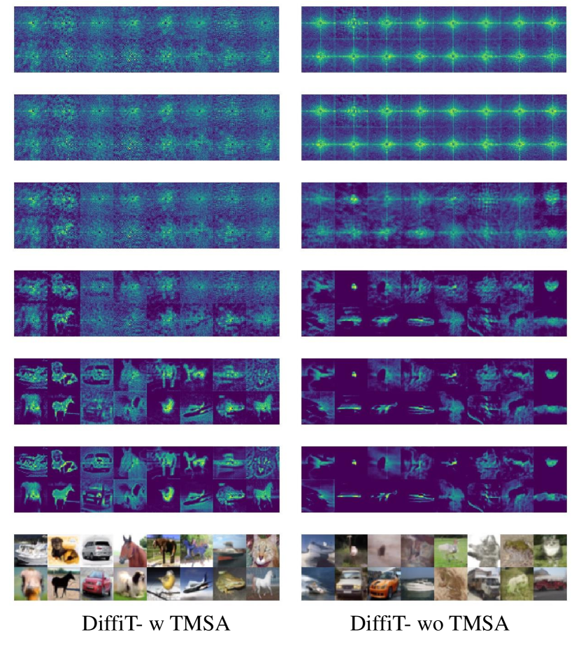
Figure 7: Side-by-side qualitative comparison of attention maps during the denoising process for models with and without TMSA. The denoising process starts at the top row.

5.5 Visualization of Self-Attention Maps

One of our key motivations in proposing TMSA is to allow the self-attention module to adapt its behavior dynamically for different stages of the denoising process. In Fig. 7, we demonstrate a qualitative comparison of self-attention maps. Although the attention maps without TMSA change in accordance to noise information, they lack fine-grained object details that are perfectly captured by TMSA.

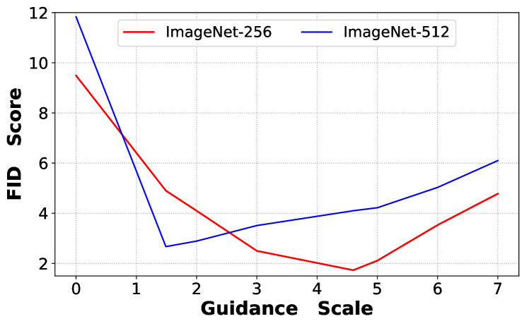
Figure 8: Effect of classifier-free guidance scale on FID score for ImageNet-256 and ImageNet-512 experiments with the latent DiffiT model.

5.6 Effect of Classifier-Free Guidance

We investigate the effect of classifier-free guidance scale on the quality of generated samples in terms of FID score. For ImageNet-256 experiment, we used the improved classifier-free guidance [21] which uses a power-cosine schedule to increase the diversity of generated images in early sampling stages. This scheme was not used for ImageNet-512 experiment, since it did not result in any significant improvements. As shown in Fig. 5.6, the guidance scales of 4.6 and 1.49 correspond to best FID scores of 1.73 and 2.67 for ImageNet-256 and ImageNet-512 experiments, respectively. Increasing the guidance scale beyond these values result in degradation of FID score.

6 Conclusion

In this work, we presented Diffusion Vision Transformers (DiffiT) which is a novel transformer-based model for diffusion-based image generation. The proposed DiffiT model unifies the design pattern of denoising diffusion architectures. We proposed a novel time-dependent self-attention layer that jointly learns both spatial and temporal dependencies. Our proposed self-attention allows for capturing short and long-range information in different time steps. Analysis of time-dependent self-attention maps reveals strong localization and dynamic temporal behavior over sampling steps. We introduced the latent DiffiT for high-resolution image generation. We have evaluated the effectiveness of DiffiT using both image and latent space experiments.

G Ablation

G.1 Time Token in TMSA

We investigate if treating time embedding as a seperate token in TMSA maybe a beneficial choice. Specifically, we apply self-attention to spatial and time tokens separately to understand the impact of decoupling them. As shown in Table S.1, we observe the degradation of performance for CIFAR10, FFHQ64 datasets, in terms of FID score. Hence, the decoupling of spatial and temporal information in TMSA leads to sub-optimal performance.

Model	TMSA Design	CIFAR10	FFHQ64
DiffiT	Separate	2.28	2.59
DiffiT	Mixed	1.95	2.22

Table S.1: Ablation study for the impact of decoupling time and spatial tokens in TMSA on FID score. Experiments are conducted on CIFAR10 [43] and FFHQ-64 [32] datasets.

G.2 Sensitivity to Time Embedding

We study the sensitivity of DiffiT model to different time embeddings representations such as Fourier and positional time embeddings. As shown in Table S.2, using a Fourier time embedding leads to degradation of performance in terms of FID score for both CIFAR10 [43] and FFHQ-64 [32] datasets.

Model	Time Embedding	CIFAR10	FFHQ64
DiffiT	Fourier	2.02	2.37
DiffiT	Positional	1.95	2.22

Table S.2: Ablation study for the impact of different time s on FID score. Experiments are conducted on CIFAR10 [43] and FFHQ-64 [32] datasets.

G.3 Comparison to DiT and LDM

On contrary to LDM [56] and DiT [52], the latent DiffiT does not rely on shift and scale, as in AdaLN [52], or concatenation to incorporate time embedding into the denoising networks. However, DiffiT uses a time-dependent self-attention (i.e. TMSA) to jointly learn the spatial and temporal dependencies. In addition, DiffiT proposes both image and latent space models for different image generation tasks with different resolutions with SOTA performance. Specifically, as shown in Table S.3, DiffiT significantly outperforms LDM [56] and DiT [52] by 31.26% and 51.94% in terms of FID score on ImageNet-256 [13] dataset. In addition, DiffiT outperforms DiT [52] by 13.85% on ImageNet-512 [13] dataset. Hence, these benchmarks validate the effectiveness of the proposes architecture and TMSA design in DiffiT model as opposed to previous SOTA for both CNN and Transformer-based diffusion models.

Model	Class	ImageNet-256				ImageNet-512
		FID $\downarrow$	IS $\uparrow$	Precision $\uparrow$	Recall $\uparrow$		FID $\downarrow$	IS $\uparrow$	Precision $\uparrow$	Recall $\uparrow$
LDM-4-G [56]	Diffusion	3.60	247.67	0.87	0.48		-	-	-	-
DiT-XL/2-G [52]	Diffusion	2.27	278.24	0.83	0.57		3.04	240.82	0.84	0.54
DiffiT	Diffusion	1.73	276.49	0.80	0.62		2.67	252.12	0.83	0.55

Table S.3: Comparison of image generation performance against state-of-the-art models on ImageNet-256 and ImageNet-512 dataset. The latent DiffiT model achieves SOTA performance in terms of FID score on ImageNet-256 dataset.

H Architecture

H.1 Image Space

We provide the details of blocks and their corresponding output sizes for both the encoder and decoder of the DiffiT model in Table S.4 and Table S.5, respectively. The presented architecture details denote models that are trained with 64$\times$64 resolution. Without loss of generality, the architecture can be extended for 32$\times$32 resolution. For FFHQ-64 [32] dataset, the values of $L_{1}$, $L_{2}$, $L_{3}$ and $L_{4}$ are 4, 4, 4, and 4 respectively. For CIFAR-10 [43] dataset, the architecture spans across three different resolution levels (i.e. 32, 16, 8), and the values of $L_{1}$, $L_{2}$, $L_{3}$ are 4, 4, 4 respectively. Please refer to the paper for more information regarding the architecture details.

Table S.4: Detailed description of components in DiffiT encoder for models that are trained at $64\times 64$ resolution.

Component Description	Output size
Input	$64\times 64\times 3$
Tokenizer	$64\times 64\times 128$
DiffiT ResBlock $\times L_{1}$	$64\times 64\times 128$
Downsampler	$32\times 32\times 128$
DiffiT ResBlock $\times L_{2}$	$32\times 32\times 256$
Downsampler	$16\times 16\times 128$
DiffiT ResBlock $\times L_{3}$	$16\times 16\times 256$
Downsampler	$8\times 8\times 256$
DiffiT ResBlock $\times L_{4}$	$8\times 8\times 256$

Table S.5: Detailed description of components in DiffiT decoder for models that are trained at $64\times 64$ resolution.

Component Description	Output size
Input	$8\times 8\times 256$
Upsampler	$16\times 16\times 256$
DiffiT ResBlock $\times L_{3}$	$16\times 16\times 256$
Upsampler	$32\times 32\times 256$
DiffiT ResBlock $\times L_{2}$	$32\times 32\times 256$
Upsampler	$64\times 64\times 256$
DiffiT ResBlock $\times L_{1}$	$64\times 64\times 128$
Head	$64\times 64\times 3$

H.2 Latent Space

In Fig S.1, we illustrate the architecture of the latent DiffiT model. Our model is comparable to DiT-XL/2-G variant which 032 uses a patch size of 2. Specifically, we use a depth of 30 layers with hidden size dimension of 1152, number of heads dimension of 16 and MLP ratio of 4. In addition, for the classifier-free guidance implementation, we only apply the guidance to the first three input channels with a scale of $(1+\mathbf{x})$ where $\mathbf{x}$ is the input latent.

Figure S.1: Overview of the latent DiffiT framework.

I Implementation Details

I.1 Image Space

We strictly followed the training configurations and data augmentation strategies of the EDM [34] model for the experiments on CIFAR10 [43], and FFHQ-64 [32] datasets, all in an unconditional setting. All the experiments were trained for 200000 iterations with Adam optimizer [39] and used PyTorch framework and 8 NVIDIA A100 GPUs. We used batch sizes of 512 and 256, learning rates of $1\times 10^{-3}$ and $2\times 10^{-4}$ and training images of sizes $32\times 32$ and $64\times 64$ on experiments for CIFAR10 [43] and FFHQ-64 [32] datasets, respectively.

We use the deterministic sampler of EDM [34] model with 18, 40 and 40 steps for CIFAR-10 and FFHQ-64 datasets, respectively. For FFHQ-64 dataset, our DiffiT network spans across 4 different stages with 1, 2, 2, 2 blocks at each stage. We also use window-based attention with local window size of 8 at each stage. For CIFAR-10 dataset, the DiffiT network has 3 stages with 2 blocks at each stage. Similarly, we compute attentions on local windows with size 4 at each stage. Note that for all networks, the resolution is decreased by a factor of 2 in between stages. However, except for when transitioning from the first to second stage, we keep the number of channels constant in the rest of the stages to maintain both the number of parameters and latency in our network. Furthermore, we employ traditional convolutional-based downsampling and upsampling layers for transitioning into lower or higher resolutions. We achieved similar image generation performance by using bilinear interpolation for feature resizing instead of convolution. For fair comparison, in all of our experiments, we used the FID score which is computed on 50K samples and using the training set as the reference set.

I.2 Latent Space

We employ learning rates of $3\times 10^{-4}$ and $1\times 10^{-4}$ and batch sizes of 256 and 512 for ImageNet-256 and ImageNet-512 experiments, respectively. We also use the exponential moving average (EMA) of weights using a decay of 0.9999 for both experiments. We also use the same diffusion hyper-parameters as in the ADM [14] model. For a fair comparison, we use the DDPM [25] sampler with 250 steps and report FID-50K for both ImageNet-256 and ImageNet-512 experiments.

J Qualitative Results

We illustrate visualization of generated images for CIFAR-10 [43] and FFHQ-64 [32] datasets in Figures S.2 and S.3, respectively. In addition, in Figures S.4,  S.5,  S.6 and  S.7, we visualize the the generated images by the latent DiffiT model for ImageNet-512 [13] dataset. Similarly, the generated images for ImageNet-256 [13] are shown in Figures  S.8, S.9 and S.10. We observe that the proposed DiffiT model is capable of capturing fine-grained details and produce high fidelity images across these datasets.

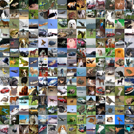
Figure S.2: Visualization of uncurated generated images for CIFAR-10 [43] dataset. Best viewed in color.

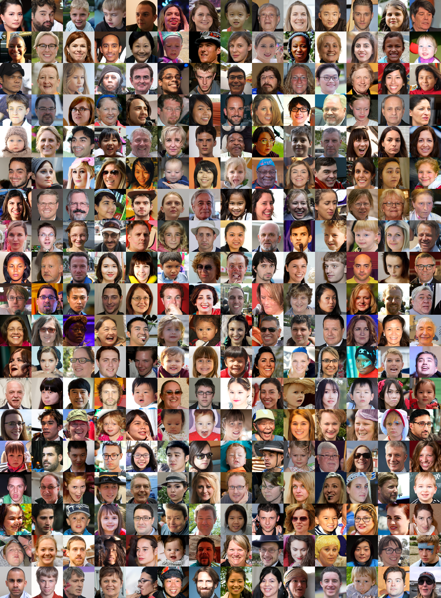
Figure S.3: Visualization of uncurated generated images for FFHQ-64 [32] dataset. Best viewed in color.

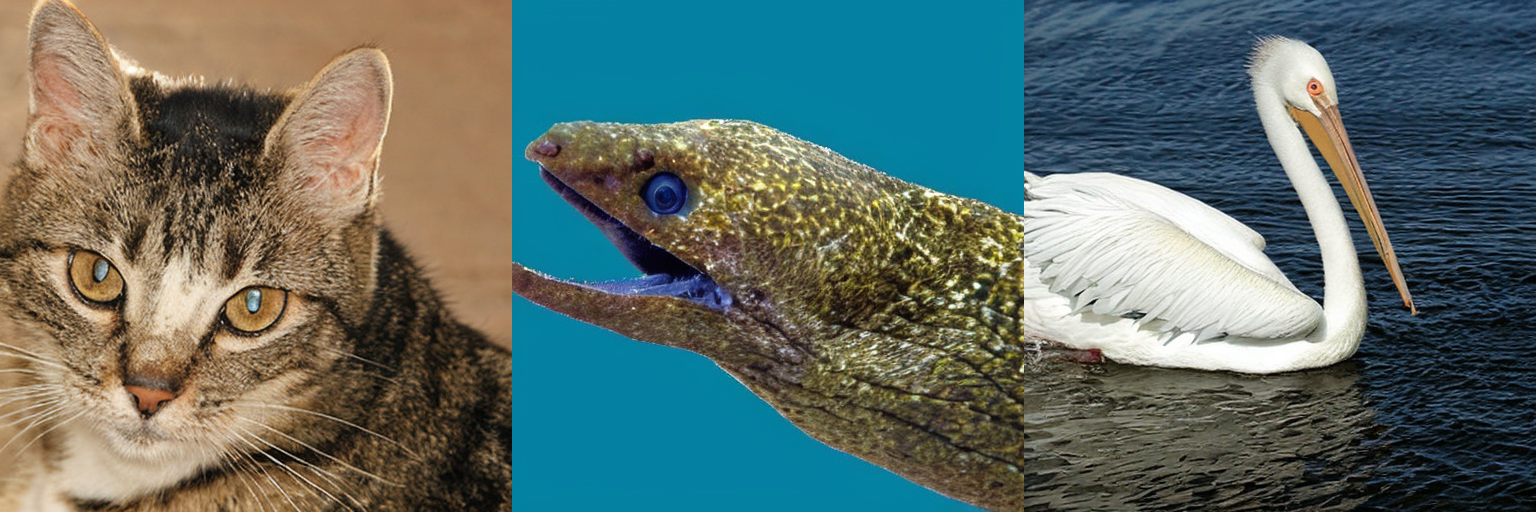
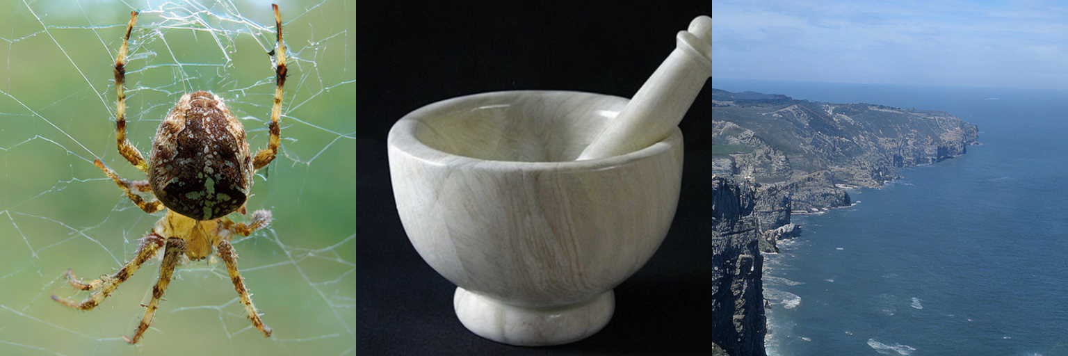
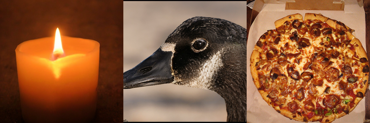
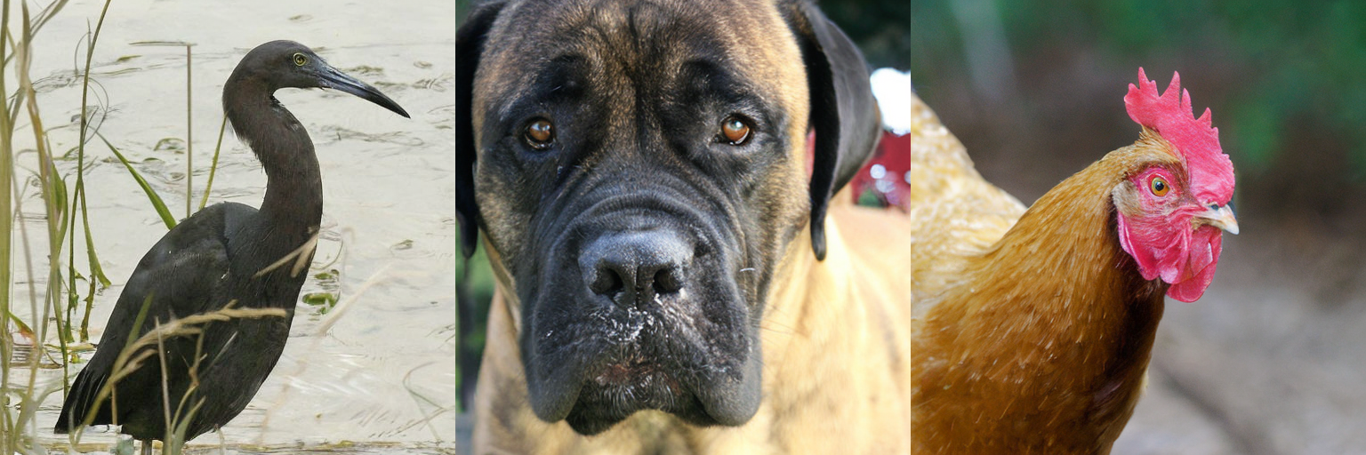
Figure S.4: Visualization of uncurated generated 512$\times$512 images on ImageNet [13] dataset by latent DiffiT model. Images are randomly sampled. Best viewed in color.

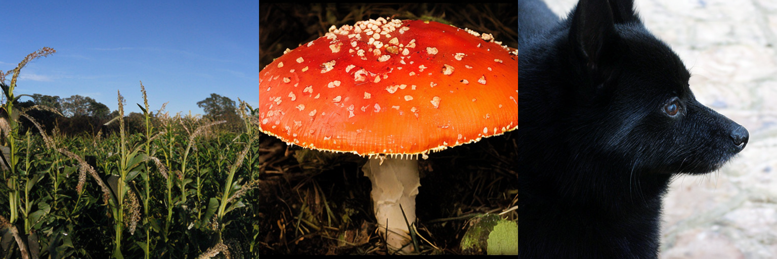
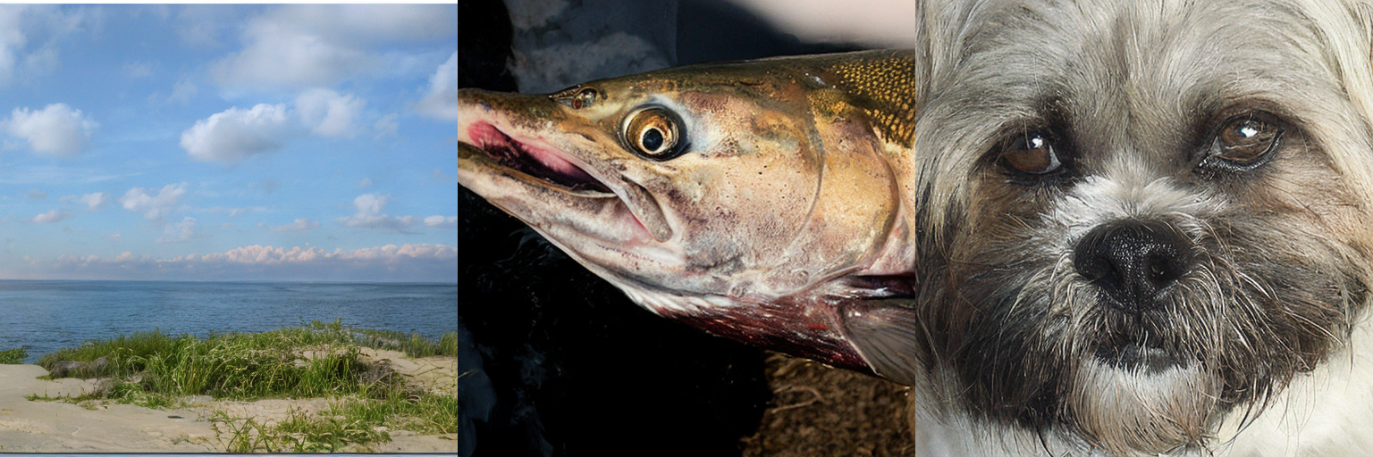
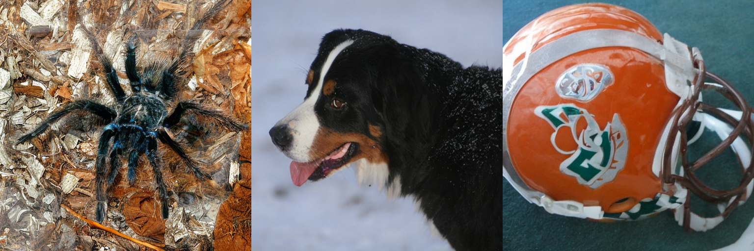
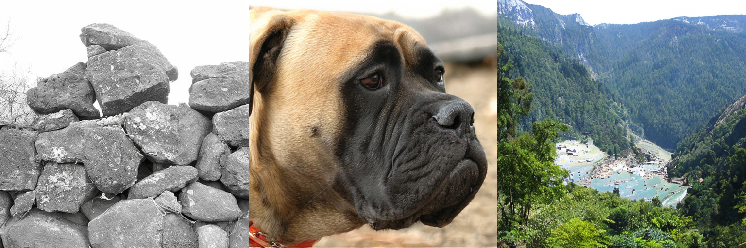
Figure S.5: Visualization of uncurated generated 512$\times$512 images on ImageNet [13] dataset by latent DiffiT model. Images are randomly sampled. Best viewed in color.

Figure S.6: Visualization of uncurated generated 512$\times$512 images on ImageNet [13] dataset by latent DiffiT model. Images are randomly sampled. Best viewed in color.

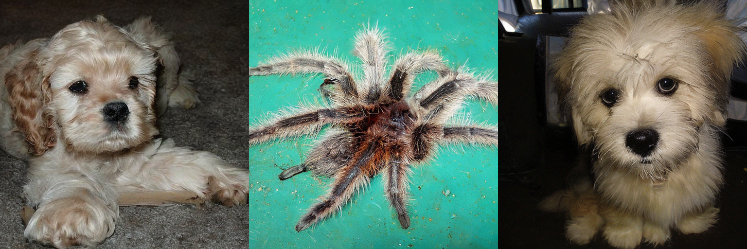
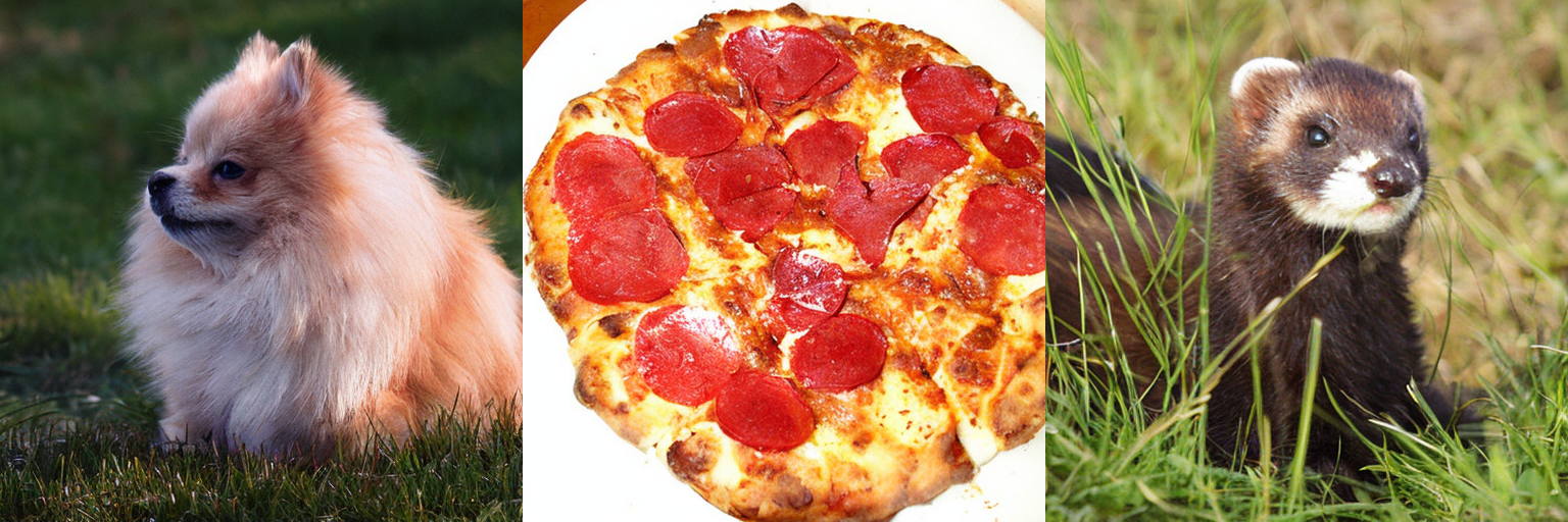
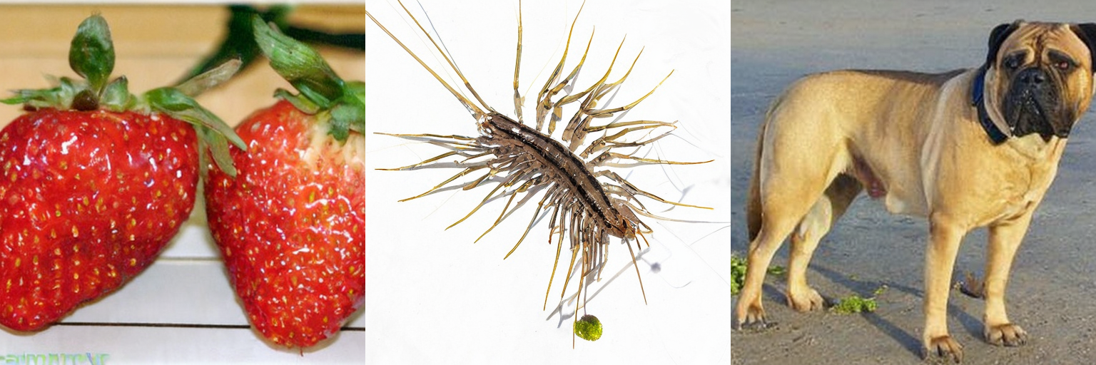
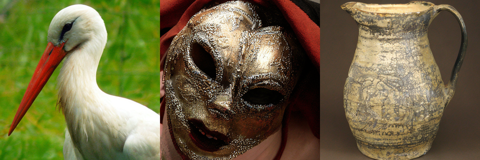
Figure S.7: Visualization of uncurated generated 512$\times$512 images on ImageNet [13] dataset by latent DiffiT model. Images are randomly sampled. Best viewed in color.

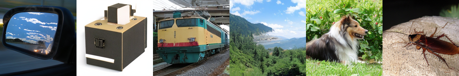
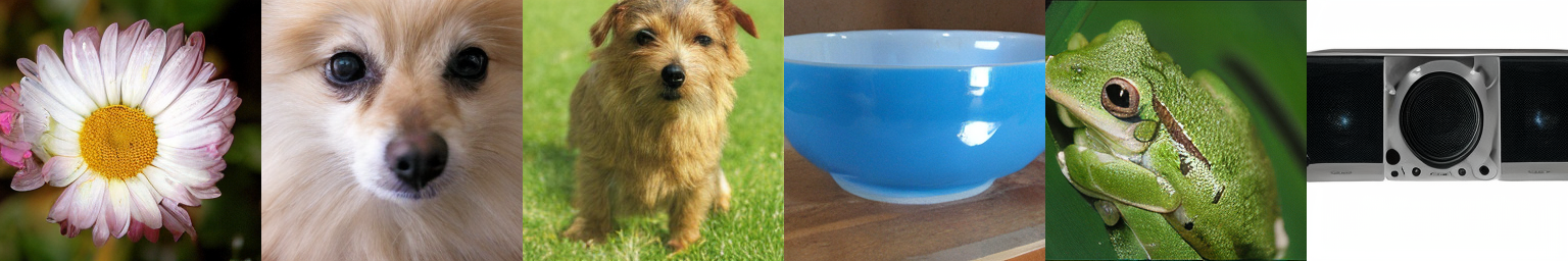
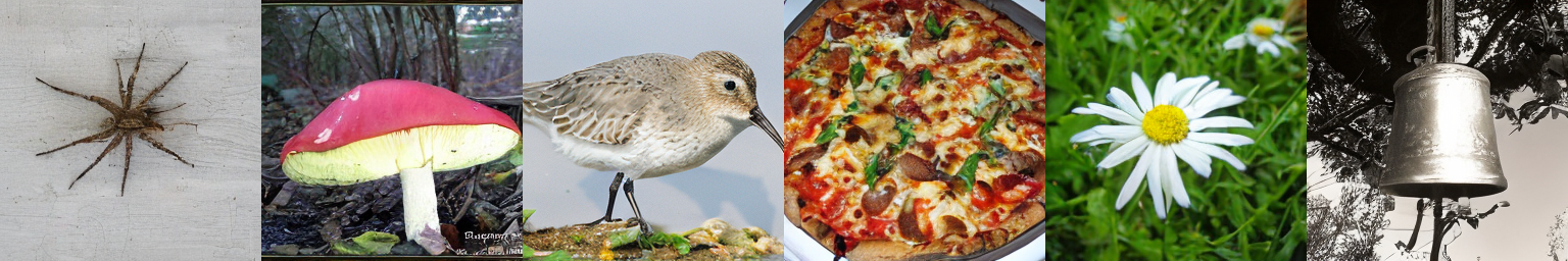
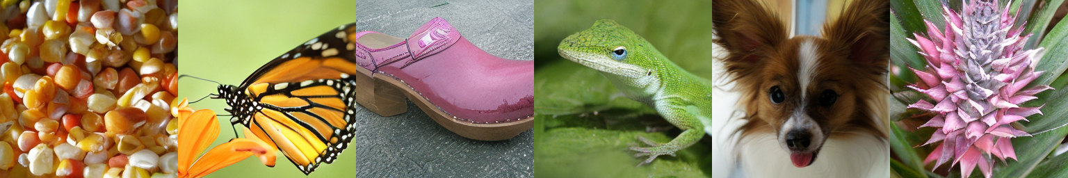
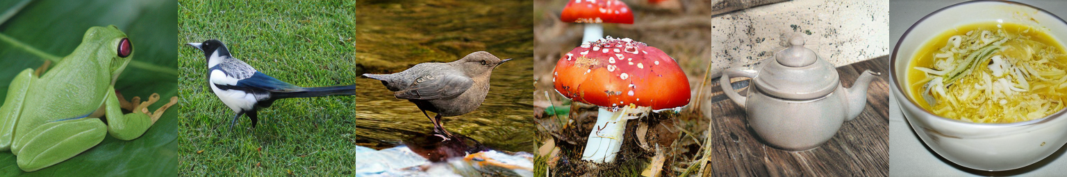
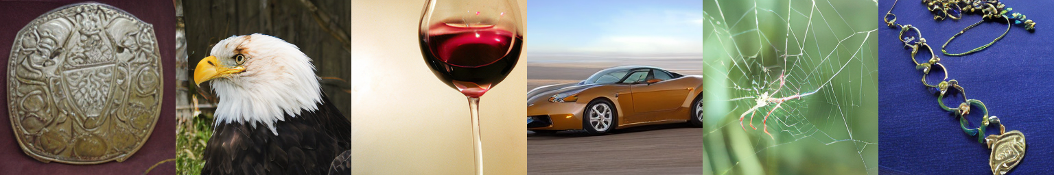
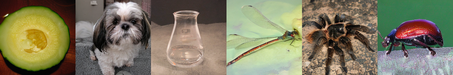
Figure S.8: Visualization of uncurated generated 256$\times$256 images on ImageNet [13] dataset by latent DiffiT model. Images are randomly sampled. Best viewed in color.

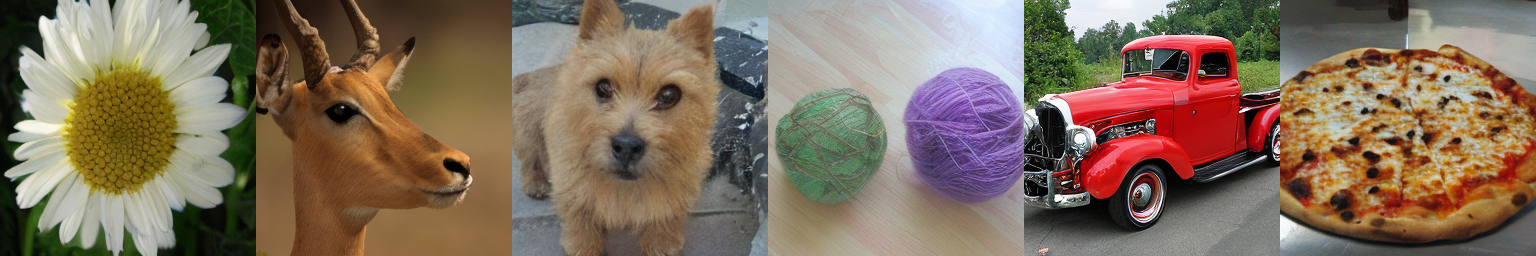
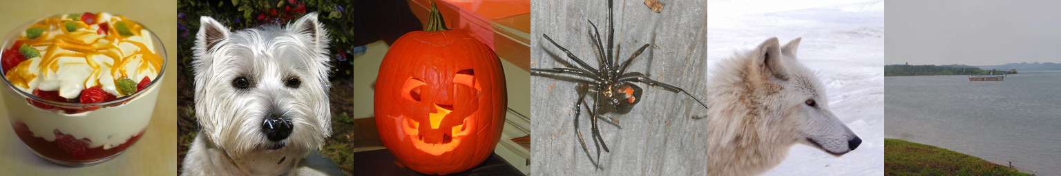
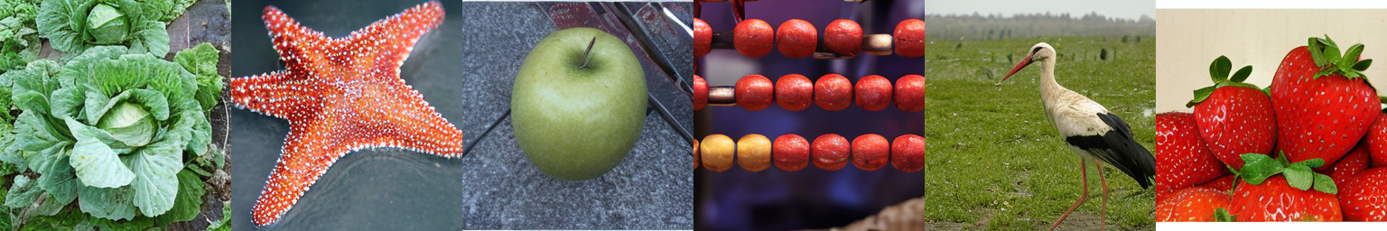
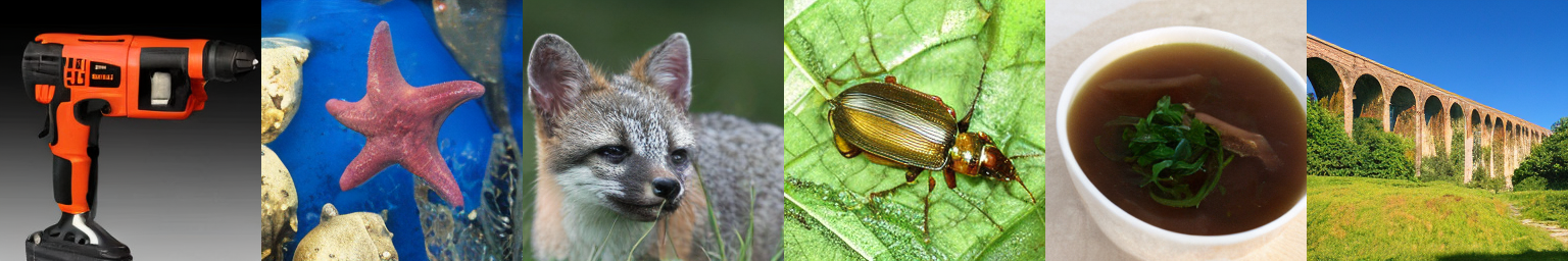
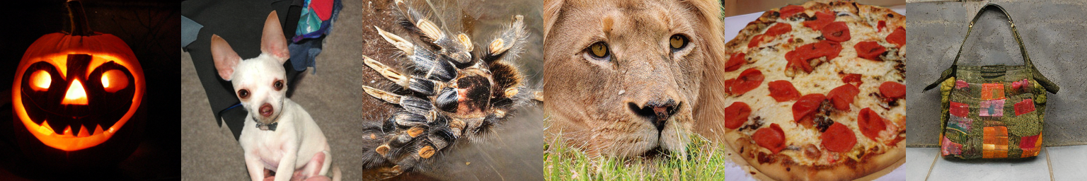
Figure S.9: Visualization of uncurated generated 256$\times$256 images on ImageNet [13] dataset by latent DiffiT model. Images are randomly sampled. Best viewed in color.

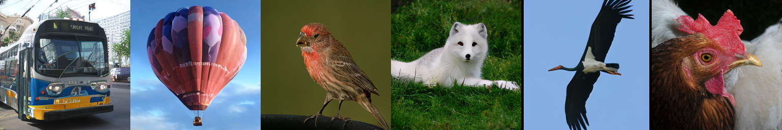
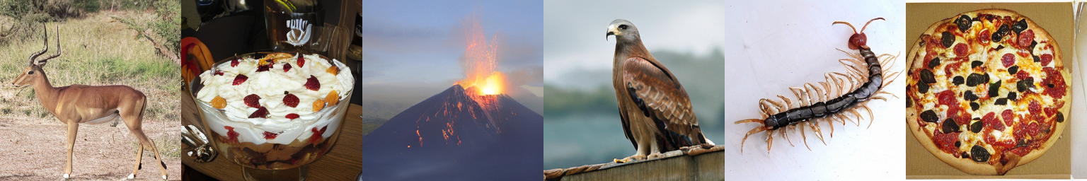
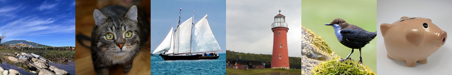
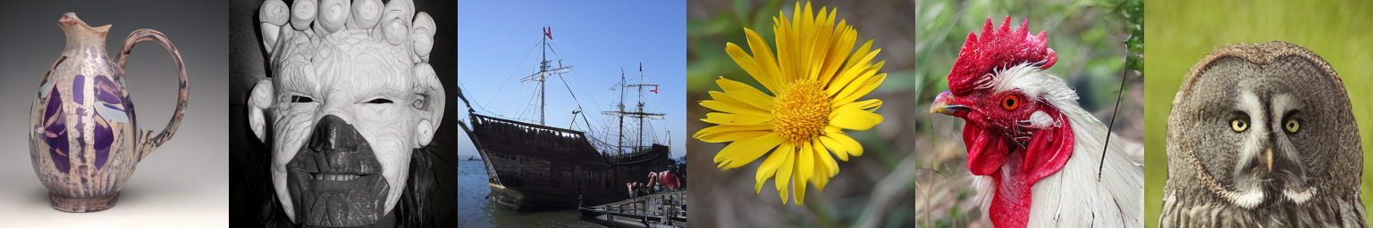
Figure S.10: Visualization of uncurated generated 256$\times$256 images on ImageNet [13] dataset by latent DiffiT model. Images are randomly sampled. Best viewed in color.

References

- Anderson [1982] Brian DO Anderson. Reverse-time diffusion equation models. Stochastic Processes and their Applications, 12(3):313–326, 1982.
- Aneja et al. [2021] Jyoti Aneja, Alex Schwing, Jan Kautz, and Arash Vahdat. A contrastive learning approach for training variational autoencoder priors. Advances in neural information processing systems, 34:480–493, 2021.
- Avrahami et al. [2022] Omri Avrahami, Dani Lischinski, and Ohad Fried. Blended diffusion for text-driven editing of natural images. In Proc. CVPR, 2022.
- Avrahami et al. [2023] Omri Avrahami, Ohad Fried, and Dani Lischinski. Blended latent diffusion. ACM Transactions on Graphics (TOG), 42(4):1–11, 2023.
- Ba et al. [2016] Jimmy Lei Ba, Jamie Ryan Kiros, and Geoffrey E Hinton. Layer normalization. arXiv preprint arXiv:1607.06450, 2016.
- Balaji et al. [2022] Yogesh Balaji, Seungjun Nah, Xun Huang, Arash Vahdat, Jiaming Song, Karsten Kreis, Miika Aittala, Timo Aila, Samuli Laine, Bryan Catanzaro, et al. ediffi: Text-to-image diffusion models with an ensemble of expert denoisers. arXiv preprint arXiv:2211.01324, 2022.
- Bao et al. [2022] Fan Bao, Chongxuan Li, Yue Cao, and Jun Zhu. All are worth words: a vit backbone for score-based diffusion models. In NeurIPS 2022 Workshop on Score-Based Methods, 2022.
- Brock et al. [2018] Andrew Brock, Jeff Donahue, and Karen Simonyan. Large scale gan training for high fidelity natural image synthesis. arXiv preprint arXiv:1809.11096, 2018.
- Chang et al. [2022] Huiwen Chang, Han Zhang, Lu Jiang, Ce Liu, and William T Freeman. Maskgit: Masked generative image transformer. In Proceedings of the IEEE/CVF Conference on Computer Vision and Pattern Recognition, pages 11315–11325, 2022.
- Chen et al. [2020] Mark Chen, Alec Radford, Rewon Child, Jeffrey Wu, Heewoo Jun, David Luan, and Ilya Sutskever. Generative pretraining from pixels. In International Conference on Machine Learning, pages 1691–1703. PMLR, 2020.
- Choi et al. [2022] Jooyoung Choi, Jungbeom Lee, Chaehun Shin, Sungwon Kim, Hyunwoo Kim, and Sungroh Yoon. Perception prioritized training of diffusion models. In Proceedings of the IEEE/CVF Conference on Computer Vision and Pattern Recognition, pages 11472–11481, 2022.
- Couairon et al. [2022] Guillaume Couairon, Jakob Verbeek, Holger Schwenk, and Matthieu Cord. DiffEdit: Diffusion-based semantic image editing with mask guidance. arXiv preprint arXiv:2210.11427, 2022.
- Deng et al. [2009] Jia Deng, Wei Dong, Richard Socher, Li-Jia Li, Kai Li, and Li Fei-Fei. Imagenet: A large-scale hierarchical image database. In 2009 IEEE conference on computer vision and pattern recognition, pages 248–255. Ieee, 2009.
- Dhariwal and Nichol [2021] Prafulla Dhariwal and Alexander Nichol. Diffusion models beat gans on image synthesis. Advances in Neural Information Processing Systems, 34:8780–8794, 2021.
- Ding et al. [2021] Ming Ding, Zhuoyi Yang, Wenyi Hong, Wendi Zheng, Chang Zhou, Da Yin, Junyang Lin, Xu Zou, Zhou Shao, Hongxia Yang, et al. Cogview: Mastering text-to-image generation via transformers. Advances in Neural Information Processing Systems, 34:19822–19835, 2021.
- Ding et al. [2022] Ming Ding, Wendi Zheng, Wenyi Hong, and Jie Tang. Cogview2: Faster and better text-to-image generation via hierarchical transformers. Advances in Neural Information Processing Systems, 35:16890–16902, 2022.
- Dockhorn et al. [2021] Tim Dockhorn, Arash Vahdat, and Karsten Kreis. Score-Based generative modeling with Critically-Damped langevin diffusion. arXiv preprint arXiv:2112.07068, 2021.
- Dosovitskiy et al. [2020] Alexey Dosovitskiy, Lucas Beyer, Alexander Kolesnikov, Dirk Weissenborn, Xiaohua Zhai, Thomas Unterthiner, Mostafa Dehghani, Matthias Minderer, Georg Heigold, Sylvain Gelly, et al. An image is worth 16x16 words: Transformers for image recognition at scale. In International Conference on Learning Representations, 2020.
- Elfwing et al. [2018] Stefan Elfwing, Eiji Uchibe, and Kenji Doya. Sigmoid-weighted linear units for neural network function approximation in reinforcement learning. Neural Networks, 107:3–11, 2018.
- Gal et al. [2022] Rinon Gal, Yuval Alaluf, Yuval Atzmon, Or Patashnik, Amit H. Bermano, Gal Chechik, and Daniel Cohen-Or. An image is worth one word: Personalizing text-to-image generation using textual inversion. arXiv preprint arXiv:2208.01618, 2022.
- Gao et al. [2023] Shanghua Gao, Pan Zhou, Ming-Ming Cheng, and Shuicheng Yan. Masked diffusion transformer is a strong image synthesizer. arXiv preprint arXiv:2303.14389, 2023.
- Gong et al. [2019] Xinyu Gong, Shiyu Chang, Yifan Jiang, and Zhangyang Wang. Autogan: Neural architecture search for generative adversarial networks. In Proceedings of the IEEE/CVF International Conference on Computer Vision, pages 3224–3234, 2019.
- Goodfellow et al. [2014] Ian Goodfellow, Jean Pouget-Abadie, Mehdi Mirza, Bing Xu, David Warde-Farley, Sherjil Ozair, Aaron Courville, and Yoshua Bengio. Generative adversarial nets. In Advances in neural information processing systems, pages 2672–2680, 2014.
- Grenander and Miller [1994] Ulf Grenander and Michael I Miller. Representations of knowledge in complex systems. Journal of the Royal Statistical Society: Series B (Methodological), 56(4):549–581, 1994.
- Ho et al. [2020] Jonathan Ho, Ajay Jain, and Pieter Abbeel. Denoising diffusion probabilistic models. arXiv preprint arXiv:2006.11239, 2020.
- Ho et al. [2022] Jonathan Ho, William Chan, Chitwan Saharia, Jay Whang, Ruiqi Gao, Alexey Gritsenko, Diederik P Kingma, Ben Poole, Mohammad Norouzi, David J. Fleet, and Tim Salimans. Imagen Video: High definition video generation with diffusion models. arXiv preprint arXiv:2210.02303, 2022.
- Hong et al. [2022] Wenyi Hong, Ming Ding, Wendi Zheng, Xinghan Liu, and Jie Tang. Cogvideo: Large-scale pretraining for text-to-video generation via transformers. arXiv preprint arXiv:2205.15868, 2022.
- Hoogeboom et al. [2023] Emiel Hoogeboom, Jonathan Heek, and Tim Salimans. simple diffusion: End-to-end diffusion for high resolution images. arXiv preprint arXiv:2301.11093, 2023.
- Hudson and Zitnick [2021] Drew A Hudson and Larry Zitnick. Generative adversarial transformers. In International conference on machine learning, pages 4487–4499. PMLR, 2021.
- Hyvärinen [2005] Aapo Hyvärinen. Estimation of non-normalized statistical models by score matching. JMLR, 6(24):695–709, 2005.
- Jiang et al. [2021] Yifan Jiang, Shiyu Chang, and Zhangyang Wang. Transgan: Two transformers can make one strong gan. arXiv preprint arXiv:2102.07074, 2021.
- Karras et al. [2019] Tero Karras, Samuli Laine, and Timo Aila. A style-based generator architecture for generative adversarial networks. In Proceedings of the IEEE/CVF conference on computer vision and pattern recognition, pages 4401–4410, 2019.
- Karras et al. [2020] Tero Karras, Miika Aittala, Janne Hellsten, Samuli Laine, Jaakko Lehtinen, and Timo Aila. Training generative adversarial networks with limited data. Advances in neural information processing systems, 33:12104–12114, 2020.
- Karras et al. [2022] Tero Karras, Miika Aittala, Timo Aila, and Samuli Laine. Elucidating the design space of diffusion-based generative models. In Proc. NeurIPS, 2022.
- Kawar et al. [2022a] Bahjat Kawar, Michael Elad, Stefano Ermon, and Jiaming Song. Denoising diffusion restoration models. arXiv preprint arXiv:2201.11793, 2022a.
- Kawar et al. [2022b] Bahjat Kawar, Jiaming Song, Stefano Ermon, and Michael Elad. Jpeg artifact correction using denoising diffusion restoration models. arXiv preprint arXiv:2209.11888, 2022b.
- Kawar et al. [2022c] Bahjat Kawar, Shiran Zada, Oran Lang, Omer Tov, Huiwen Chang, Tali Dekel, Inbar Mosseri, and Michal Irani. Imagic: Text-based real image editing with diffusion models. arXiv preprint arXiv:2210.09276, 2022c.
- Kim et al. [2022] Dongjun Kim, Byeonghu Na, Se Jung Kwon, Dongsoo Lee, Wanmo Kang, and Il-Chul Moon. Maximum likelihood training of implicit nonlinear diffusion models. arXiv preprint arXiv:2205.13699, 2022.
- Kingma and Ba [2014] Diederik P Kingma and Jimmy Ba. Adam: A method for stochastic optimization. arXiv preprint arXiv:1412.6980, 2014.
- Kingma and Welling [2013] Diederik P Kingma and Max Welling. Auto-Encoding variational bayes. arXiv preprint arXiv:1312.6114v10, 2013.
- Kong et al. [2020] Zhifeng Kong, Wei Ping, Jiaji Huang, Kexin Zhao, and Bryan Catanzaro. Diffwave: A versatile diffusion model for audio synthesis. arXiv preprint arXiv:2009.09761, 2020.
- Kreis et al. [2022] Karsten Kreis, Ruiqi Gao, and Arash Vahdat. CVPR tutorial on denoising diffusion-based generative modeling: Foundations and applications. https://cvpr2022-tutorial-diffusion-models.github.io/, 2022.
- Krizhevsky et al. [2009] Alex Krizhevsky, Geoffrey Hinton, et al. Learning multiple layers of features from tiny images. 2009.
- Lee et al. [2022] Doyup Lee, Chiheon Kim, Saehoon Kim, Minsu Cho, and Wook-Shin Han. Autoregressive image generation using residual quantization. In Proceedings of the IEEE/CVF Conference on Computer Vision and Pattern Recognition, pages 11523–11532, 2022.
- Lee et al. [2021] Kwonjoon Lee, Huiwen Chang, Lu Jiang, Han Zhang, Zhuowen Tu, and Ce Liu. Vitgan: Training gans with vision transformers. arXiv preprint arXiv:2107.04589, 2021.
- Li et al. [2021] Shanda Li, Xiangning Chen, Di He, and Cho-Jui Hsieh. Can vision transformers perform convolution? arXiv preprint arXiv:2111.01353, 2021.
- Li et al. [2022] Xiang Lisa Li, John Thickstun, Ishaan Gulrajani, Percy Liang, and Tatsunori B Hashimoto. Diffusion-lm improves controllable text generation. arXiv preprint arXiv:2205.14217, 2022.
- Luhman and Luhman [2022] Troy Luhman and Eric Luhman. Improving diffusion model efficiency through patching. arXiv preprint arXiv:2207.04316, 2022.
- Meng et al. [2021] Chenlin Meng, Yutong He, Yang Song, Jiaming Song, Jiajun Wu, Jun-Yan Zhu, and Stefano Ermon. Sdedit: Guided image synthesis and editing with stochastic differential equations. arXiv preprint arXiv:2108.01073, 2021.
- Nie et al. [2022] Weili Nie, Brandon Guo, Yujia Huang, Chaowei Xiao, Arash Vahdat, and Anima Anandkumar. Diffusion models for adversarial purification. In Proc. ICML, 2022.
- Park and Kim [2022] Jeeseung Park and Younggeun Kim. Styleformer: Transformer based generative adversarial networks with style vector. In Proceedings of the IEEE/CVF Conference on Computer Vision and Pattern Recognition, pages 8983–8992, 2022.
- Peebles and Xie [2023] William Peebles and Saining Xie. Scalable diffusion models with transformers. In Proceedings of the IEEE/CVF International Conference on Computer Vision, pages 4195–4205, 2023.
- Perez et al. [2018] Ethan Perez, Florian Strub, Harm De Vries, Vincent Dumoulin, and Aaron Courville. Film: Visual reasoning with a general conditioning layer. In Proceedings of the AAAI Conference on Artificial Intelligence, 2018.
- Ramesh et al. [2022] Aditya Ramesh, Prafulla Dhariwal, Alex Nichol, Casey Chu, and Mark Chen. Hierarchical text-conditional image generation with CLIP latents. arXiv preprint arXiv:2204.06125, 2022.
- Rombach and Esser [2022] Robin Rombach and Patrick Esser. Stable diffusion v1-4. https://huggingface.co/CompVis/stable-diffusion-v1-4, 2022.
- Rombach et al. [2022] Robin Rombach, Andreas Blattmann, Dominik Lorenz, Patrick Esser, and Björn Ommer. High-resolution image synthesis with latent diffusion models. In Proceedings of the IEEE/CVF Conference on Computer Vision and Pattern Recognition, pages 10684–10695, 2022.
- Ronneberger et al. [2015] Olaf Ronneberger, Philipp Fischer, and Thomas Brox. U-Net: Convolutional networks for biomedical image segmentation. arXiv preprint arXiv:1505.04597, 2015.
- Ruiz et al. [2022] Nataniel Ruiz, Yuanzhen Li, Varun Jampani, Yael Pritch, Michael Rubinstein, and Kfir Aberman. DreamBooth: Fine tuning text-to-image diffusion models for subject-driven generation. arXiv preprint arXiv:2208.12242, 2022.
- Saharia et al. [2022] Chitwan Saharia, William Chan, Saurabh Saxena, Lala Li, Jay Whang, Emily Denton, Seyed Kamyar Seyed Ghasemipour, Burcu Karagol Ayan, S Sara Mahdavi, Rapha Gontijo Lopes, et al. Photorealistic text-to-image diffusion models with deep language understanding. arXiv preprint arXiv:2205.11487, 2022.
- Salimans and Ho [2022] Tim Salimans and Jonathan Ho. Progressive distillation for fast sampling of diffusion models. arXiv preprint arXiv:2202.00512, 2022.
- Sauer et al. [2022] Axel Sauer, Katja Schwarz, and Andreas Geiger. Stylegan-xl: Scaling stylegan to large diverse datasets. In ACM SIGGRAPH 2022 conference proceedings, pages 1–10, 2022.
- Shaw et al. [2018] Peter Shaw, Jakob Uszkoreit, and Ashish Vaswani. Self-attention with relative position representations. arXiv preprint arXiv:1803.02155, 2018.
- Sinha et al. [2021] Abhishek Sinha, Jiaming Song, Chenlin Meng, and Stefano Ermon. D2c: Diffusion-decoding models for few-shot conditional generation. Advances in Neural Information Processing Systems, 34:12533–12548, 2021.
- Sohl-Dickstein et al. [2015] Jascha Sohl-Dickstein, Eric A Weiss, Niru Maheswaranathan, and Surya Ganguli. Deep unsupervised learning using nonequilibrium thermodynamics. arXiv preprint arXiv:1503.03585, 2015.
- Song et al. [2021a] Jiaming Song, Chenlin Meng, and Stefano Ermon. Denoising diffusion implicit models. In International Conference on Learning Representations, 2021a.
- Song et al. [2021b] Yang Song, Jascha Sohl-Dickstein, Diederik P Kingma, Abhishek Kumar, Stefano Ermon, and Ben Poole. Score-based generative modeling through stochastic differential equations. In International Conference on Learning Representations, 2021b.
- Tashiro et al. [2021] Yusuke Tashiro, Jiaming Song, Yang Song, and Stefano Ermon. Csdi: Conditional score-based diffusion models for probabilistic time series imputation. Advances in Neural Information Processing Systems, 34:24804–24816, 2021.
- Vahdat and Kautz [2020] Arash Vahdat and Jan Kautz. Nvae: A deep hierarchical variational autoencoder. Advances in neural information processing systems, 33:19667–19679, 2020.
- Vahdat et al. [2021] Arash Vahdat, Karsten Kreis, and Jan Kautz. Score-based generative modeling in latent space. arXiv preprint arXiv:2106.05931, 2021.
- Valevski et al. [2022] Dani Valevski, Matan Kalman, Yossi Matias, and Yaniv Leviathan. UniTune: Text-driven image editing by fine tuning an image generation model on a single image. arXiv preprint arXiv:2210.09477, 2022.
- Vincent [2011] Pascal Vincent. A connection between score matching and denoising autoencoders. Neural computation, 23(7):1661–1674, 2011.
- Wang et al. [2020] Sinong Wang, Belinda Li, Madian Khabsa, Han Fang, and Hao Ma. Linformer: Self-attention with linear complexity. arXiv preprint arXiv:2006.04768, 2020.
- Wu and He [2018] Yuxin Wu and Kaiming He. Group normalization. arXiv preprint arXiv:1803.08494, 2018.
- Xu et al. [2022] Minkai Xu, Lantao Yu, Yang Song, Chence Shi, Stefano Ermon, and Jian Tang. GeoDiff: A geometric diffusion model for molecular conformation generation. In Proc. ICLR, 2022.
- Xu et al. [2021] Rui Xu, Xiangyu Xu, Kai Chen, Bolei Zhou, and Chen Change Loy. Stransgan: An empirical study on transformer in gans. arXiv preprint arXiv:2110.13107, 2021.
- Yang et al. [2022] Xiulong Yang, Sheng-Min Shih, Yinlin Fu, Xiaoting Zhao, and Shihao Ji. Your vit is secretly a hybrid discriminative-generative diffusion model. arXiv preprint arXiv:2208.07791, 2022.
- Ye et al. [2022] Mao Ye, Lemeng Wu, and Qiang Liu. First hitting diffusion models. arXiv preprint arXiv:2209.01170, 2022.
- Zeng et al. [2022] Xiaohui Zeng, Arash Vahdat, Francis Williams, Zan Gojcic, Or Litany, Sanja Fidler, and Karsten Kreis. Lion: Latent point diffusion models for 3d shape generation. In Advances in Neural Information Processing Systems (NeurIPS), 2022.
- Zhang et al. [2022a] Bowen Zhang, Shuyang Gu, Bo Zhang, Jianmin Bao, Dong Chen, Fang Wen, Yong Wang, and Baining Guo. Styleswin: Transformer-based gan for high-resolution image generation. In Proceedings of the IEEE/CVF Conference on Computer Vision and Pattern Recognition, pages 11304–11314, 2022a.
- Zhang et al. [2021] Han Zhang, Weichong Yin, Yewei Fang, Lanxin Li, Boqiang Duan, Zhihua Wu, Yu Sun, Hao Tian, Hua Wu, and Haifeng Wang. Ernie-vilg: Unified generative pre-training for bidirectional vision-language generation. arXiv preprint arXiv:2112.15283, 2021.
- Zhang et al. [2022b] Qinsheng Zhang, Molei Tao, and Yongxin Chen. gddim: Generalized denoising diffusion implicit models. arXiv preprint arXiv:2206.05564, 2022b.
- Zhao et al. [2021] Long Zhao, Zizhao Zhang, Ting Chen, Dimitris Metaxas, and Han Zhang. Improved transformer for high-resolution gans. Advances in Neural Information Processing Systems, 34:18367–18380, 2021.
- Zheng et al. [2021] Sixiao Zheng, Jiachen Lu, Hengshuang Zhao, Xiatian Zhu, Zekun Luo, Yabiao Wang, Yanwei Fu, Jianfeng Feng, Tao Xiang, Philip HS Torr, et al. Rethinking semantic segmentation from a sequence-to-sequence perspective with transformers. In Proceedings of the IEEE/CVF Conference on Computer Vision and Pattern Recognition, pages 6881–6890, 2021.
- Zhou et al. [2021] Linqi Zhou, Yilun Du, and Jiajun Wu. 3D shape generation and completion through Point-Voxel diffusion. arXiv preprint arXiv:2104.03670, 2021.