Distance function for spike prediction

Abstract

Approaches to predicting neuronal spike responses commonly use a Poisson learning objective. This objective quantizes responses into spike counts within a fixed summation interval, typically on the order of $10100$ milliseconds in duration; however, neuronal responses are often time accurate down to a few milliseconds, and at these timescales, Poisson models typically perform poorly. To overcome this limitation, we propose the concept of a spike distance function that maps points in time to the temporal distance to the nearest spike. We show that neural networks can be trained to approximate spike distance functions, and we present an efficient algorithm for inferring spike trains from the outputs of these models. Using recordings of chicken and frog retinal ganglion cells responding to visual stimuli, we compare the performance of our approach to Poisson models trained with various summation intervals. We show that our approach outperforms the standard Poisson approach at spike train inference.

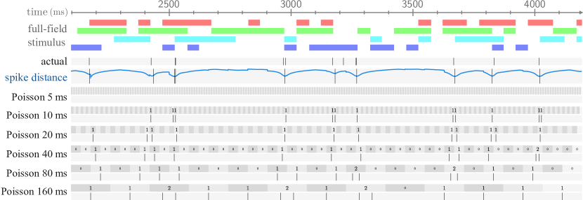
Figure 1: Spike prediction using spike distance. The output of a spike distance model (depicted by the blue line) can be used to precisely predict spikes. On the other hand, the standard Poisson approach, which relies on spike counts within fixed intervals, suffers from a trade-off: longer intervals prevent precise spike localization, while shorter intervals cause maximum likelihood predictions to tend towards 0 for all time steps.

1 Introduction

This paper proposes a new learning objective for the problem of spike prediction. Spike prediction is the task of estimating the timing of future action potentials (spikes) of a neuron; for example, given {1000} of stimulus and spike activity, predict the next {80} of spike activity. The task is illustrated in Figure 2.

Figure 2: Spike prediction task: predict future spikes given stimulus and spike history. For this work, stimulus history is a 1-second snippet of a widefield stimulus at four wavebands. The prediction duration is not fixed—several durations are explored. Information about the stimulus after $t=0$ is not available to the model, matching the task faced by retinal prosthetic devices.

A widely used approach to spike prediction is to train a model to predict the number of spikes that will occur within a fixed time interval. A probabilistic motivation is often given by describing the neuron’s output as a Poisson process. In this setting, the model’s output, often called the firing rate, corresponds to the single parameter of the Poisson process at a certain point in time. Training the model amounts to maximizing the likelihood of this time-varying parameter with respect to the data. Spike counts can be predicted by reading off the rounded outputs of a trained model or by sampling from Poisson distributions parameterized by the model’s outputs. For the Poisson approach, the interval length over which spikes are summed is a delicate hyperparameter that significantly impacts the behaviour of a model. In this work, we question the need for a summation interval for spike prediction.

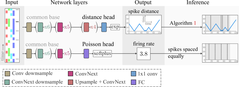
Figure 3: Overview of spike prediction for both the spike distance approach and the Poisson approach. To make the two comparable, the networks used by each approach were designed with the preponderance of weights and computation carried out using the same twelve-layer base architecture. Inference of spike times from spike distance is achieved by Algorithm 1 in Section 5.

Rather than reduce a chunk of a spike train to a single number, we choose a representation that preserves its details. Inspired by the idea of a signed distance function used in geometric modelling, we propose the idea of a spike distance function that maps points in time to the temporal distance to the nearest spike. We train neural networks to output this representation and use it to predict spike trains. An overview of the spike distance approach (still imprecisely defined for now) compared to the Poisson approach is shown in Figure 3.

We inspect the effectiveness of this new approach by comparing a neural network trained using the spike distance objective with neural networks trained using a range of Poisson objectives, each using a different summation interval. Our spike prediction dataset is formed from a multi-electrode array (MEA) recording of 60 chicken retinal ganglion cells responding to visual stimuli. We repeat our experiments for 48 frog RGCs from a separate recording.

In the next section, we present related work. We come back to set the scene more concretely by elucidating the drawbacks of the Poisson approach in Section 3 and describing the spike distance function in Section 4. How to infer spike trains from model outputs is covered in Section 5. The experiments are described in Section 6 with results appearing in Section 7 and a brief discussion following in Section 8.

2 Related work

For the task of spike prediction, the effectiveness despite simplicity of generalized linear models makes them important models to study. Using GLMs to model neurons is covered by Weber and Pillow (2017). GLMs are further relevant because their success has contributed to the popularity of the Poisson learning objective.

GLMs are effectively single-layer neural networks, and so the neural network approaches that follow can be thought of as trading the simplicity of GLMs with the increased power of deeper neural networks. McIntosh et al. (2016) used convolutional neural networks and recurrent neural networks to predict spiking behaviour of tiger salamander RGCs. In parallel, Batty et al. (2016) carried out similar work using RNNs to predict spiking behaviour of macaque RGCs. Both of these studies recorded the cells using MEAs. Cadena et al. (2019) compared CNNs trained from scratch with a fine-tuned vision model at predicting spiking behaviour of macaque V1 neurons. This study recorded cells using penetrative probes.

Stepping back, spike prediction is an example of the more general problem of localizing points in 1 or more dimensions or localizing surfaces in 2 or more dimensions and so on, of which there are other applications. Earthquake prediction faces such a problem where the task is framed as predicting the “time to failure”. Computer vision and graphics have a concept analogous to “time to failure” in the form of a signed distance function, which is effectively a “distance to surface” and is used for implicitly modelling 2D surfaces in 3D space. It is from these contexts that we draw inspiration to propose “distance to spike” as an effective tool for spike prediction.

For earthquake prediction, Rouet-Leduc et al. (2017) and Wang et al. (2022) applied machine learning to predict time-to-failure for a laboratory fault system. See the review by Ren et al. (2020) for broad coverage. Interestingly, these approaches stop at predicting time-to-failure signals and do not take the next step of inferring precise rupture times from these signals. The inference procedure described in Section 5 will work with these signals also.

In computer vision, the notion of a signed distance function is used to implicitly define surfaces. Our work to predict spike distance is analogous to the work by Zeng et al. (2017) and Dai et al. (2017) who used neural networks to represent 3D shapes using a grid of truncated signed distance values. Later work in this area has tackled the scaling issues with 3D data, such as the work by Park et al. (2019), where neural networks were given the additional job of querying the 3D representation. The directional queries of the 3D representation are conceptually similar to spike-stimulus history input that we will use to request output behaviour from our neural network model. Although not considered in this work, the creative forms of querying 3D representations, such as Sitzmann et al.’s (2021) use of Plücker coordinates, raise the question: are there other useful ways to query neural network representations for neuronal behaviour?

3 Issues with the Poisson approach

The summation interval used in the Poisson approach to spike prediction leads to a trade-off between temporal resolution and a balanced dataset. A related issue is the leniency of the loss signal within an interval and its abrupt jump at the boundaries.

The goal of having predictions with high temporal resolution encourages the choice of a shorter summation interval. Recordings of chicken RGCs show bursts of spikes with spike intervals as short as $12$ $\mathrm{m}\mathrm{s}$ (Seifert et al., 2023); and primate, salamander, cat and rabbit RGCs have been shown to have stimulus-driven variability across trials as low as {1} (Uzzell and Chichilnisky, 2004; Berry and Meister, 1998; Keat et al., 2001; Berry et al., 1997). Neurons from other brain regions also demonstrate this precision, such as neurons in the lateral geniculate nucleus of cats (Butts et al., 2011; Keat et al., 2001). This suggests that summation intervals as short as {1}ms in duration would be useful. However, decreasing the summation interval causes issues: training slows as data becomes spread over an increased number of samples; and a greater proportion of time intervals contain no spikes making it difficult to escape the trivial solution of outputting 0 for all time steps. Furthermore, after training, maximum likelihood for spike prediction becomes ineffective, as model outputs round to zero. To avoid this, summation intervals must be chosen long enough to ensure that the preponderance of intervals are not empty. However, as intervals are made larger, another drawback is encountered.

An issue that detracts from larger intervals is that movement of spikes within the summation interval does not affect the Poisson loss, and movement of spikes across the interval boundary causes the loss to abruptly change. If a summation interval of {80}ms is used, then {80}ms of neural activity will be compressed into a single scalar value—a quick burst of spikes a few milliseconds apart will be indistinguishable from the same number of spikes spread over the entire interval. In contrast, for the boundary, consider an example: a model predicts one spike in the interval $[\quantity{20}{ms},\quantity{25}{ms}]$ while the single ground truth spike falls just outside, say at {26}ms. The loss for the interval $[\quantity{20}{ms},\quantity{25}{ms}]$ will push the model’s output towards zero as strongly as had the nearest spike been at $\quantity{50}{ms}$ or later or had there been no spikes at all. Effectively, the Poisson loss has maximal leniency within the interval boundary and zero tolerance for any crossing of the boundary. Instead, it would be desirable to have a loss signal that changes in proportion to changes in spike positions. The spike distance function described next is a spike train representation with this property.

4 Spike distance

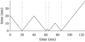
Figure 4: The spike distance in milliseconds over the interval $[0,128]$ for the spikes $[20,60,65,86]$.

A Spike distance function maps each point in time to a scalar representing the temporal distance to the nearest spike. This is either the time elapsed since the last spike or the time remaining until the next spike, whichever is less. This is an implicit representation of a set of spikes using contours. A comprehensive treatment of using implicit functions to represent points and surfaces is Osher and Fedkiw (2003).

Formally, let $S\in\mathbb{R}^{N}$ be a set $N$ of spike times. Let $I=[a,b]$ be an interval of $\mathbb{R}$. The spike distance function of $S$ on $I$ is the function $f_{S}:I\rightarrow\mathbb{R}$ is defined as:

$$f_{S}(t)=\min_{s\in S}|t-s|$$

Any interval can support a spike distance function, and this spike distance function can depend on spikes both inside and outside the interval. An example spike distance evaluated over the interval $[\quantity{0}{ms},\quantity{128}{ms}]$ for the spikes $[\quantity{20}{ms},\quantity{60}{ms},\quantity{65}{ms},\quantity{86}{ms}]$ is shown in Figure 4. From the example, it can be seen that subtle or large changes to a spike train will be reflected proportionately in the spike distance function, which was the characteristic lacking in the Poisson loss signal.

In practice, we will work with discrete arrays, and use a discrete spike distance function, $\hat{f}_{S}:\mathbb{N}\to\mathbb{R}$, where $\hat{f}_{S}$ is now parameterized by a discrete spike sequence, $S$. The discrete spike distance is covered in detail in Appendix A.10. Two other considerations, the choice of a maximum distance and the choice of the evaluation interval, are discussed in Appendix A.9.

5 Spike train inference

For the spike prediction task, we must infer a spike train from a model’s outputs. For both the spike distance model and the Poisson models this will be done autoregressively: concatenating model outputs and using previously predicted spikes as input to subsequent forward passes. The two approaches differ in how they carry out a single step—each is covered over the next two sections.

5.1 Spikes from a spike distance array

We describe spike inference from a spike distance array from the perspective of energy minimization. An array of spike distance values outputted by a model can be seen as parameterizing some function that assigns a scalar energy value to any set of spikes. Various functions are possible. We use the L2 norm between the model output and the discrete spike distance function of a candidate spike sequence. Let the model output $M=(m_{i})_{i=0}^{L-1}$ be a sequence of reals of length $L$, and let $S=(s_{i})_{i=0}^{L-1}$ be a candidate spike sequence of the same length. The energy assigned to $S$ is given by:

$$E_{M}(S)=\sum_{i=0}^{L-1}(\hat{f}_{S}(i)-m_{i})^{2}$$ (1)

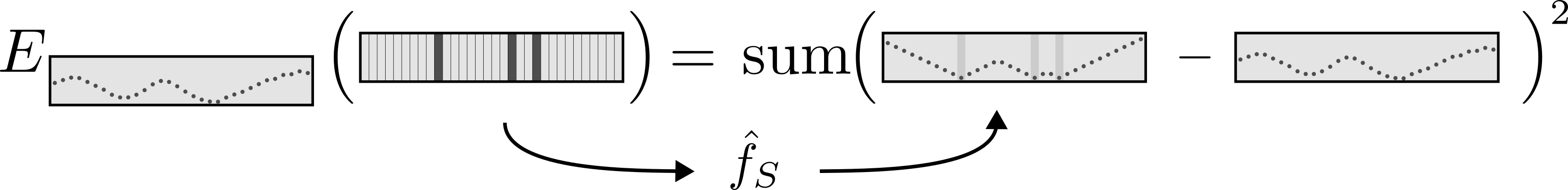
Figure 5: Visual form of Equation 1. The discrete spike distance, $\hat{f}_{S}$, is described in Appendix A.10.

The energy is a measure of incompatibility between the candidate spikes and the model output (here we are following the convention that low energy values correspond to greater compatibility). Spike train inference amounts to finding the spike train with the lowest energy.

This optimization problem can be solved exactly by brute-force search. Dynamic programming can also be used, as the problem can be decomposed into left and right sub-problems. Both of these approaches were found to be too slow in practice. We propose an inexact solution, Algorithm 1, that begins by predicting a spike in every time step then iteratively refines the prediction by removing spikes.

Algorithm 1 Spike Inference Algorithm: predict a spike in every time step then iteratively remove spikes—remove if the L2 norm between the candidate and target distance arrays is lower when the spike is not present. Iterate spikes in order of the estimated effect on the error. The function SpikeDist converts a set of spikes into an array of spike distances (see Appendix A.10).

1:$w$ is the target spike distance (model output) and $s_{0}$ is the most recent “past” spike.

2:

3:function SpikeInference($w,s_{0}$)

4:     $S\leftarrow\text{indices of }w$

5:     $\textit{scores}\leftarrow w$

6:     repeat

7:         $S_{\textit{old}}\leftarrow S$

8:         for all $s\in S$ sorted by $\textit{scores}[s]$ in descending order do

9:              $err\leftarrow\textsc{L2Norm}(w,\textsc{SpikeDist}(S,s_{0})\,)$

10:              $S^{\prime}\leftarrow S\text{ with }s\text{ removed}$

11:              $err^{\prime}\leftarrow\textsc{L2Norm}(w,\textsc{SpikeDist}(S^{\prime},s_{0})\,)$

12:              $\delta\leftarrow err-err^{\prime}$

13:              $\textit{scores}[s]\leftarrow\delta$

14:              if $\delta>0$ then

15:                  $S\leftarrow S^{\prime}$                        

16:     until $S=S_{\textit{old}}$

17:     return $S$

In terms of time complexity, applying this algorithm autoregressively to infer a spike train $L\,\text{bins}$ long, broken into $N$ steps of $l\,\text{bins}$ uses $\sim Nl^{2}\log l$ compares in the worst case—this corresponds to an $l\log l$ cost of sorting that may be repeated $l$ times each inference step, of which there are $N$. Except in pathological cases, the outer loop of SpikeInference requires very few iterations—for the combined 90 minutes of spike train inference carried out on the chicken test set, no inference step required more than two iterations. Thus, with comparisons as a cost model, the algorithm’s average cost can be considered to grow linearly with the number of inference steps ($N$) and linearithmic with the resolution ($l$) of a single inference step. Figure 17 in Appendix A.8 shows inference running times on the authors’ hardware. The algorithm uses additional memory that grows linearly with $l$.

5.2 Spikes from a Poisson distribution

A Poisson distribution has a single parameter $\lambda$. A model trained with a Poisson learning objective outputs a single scalar value, $y$, which is used to parameterize a Poisson distribution by setting $\lambda=y$. From such a parameterized Poisson distribution, there are two ways to infer spikes: maximum likelihood and sampling.

Maximum likelihood prediction involves selecting the spike count with maximum probability under the Poisson distribution with parameter $\lambda=y$. By nature of the Poisson distribution, this is the value $y$. This value is rounded to produce an integer number of spikes. As the Poisson distribution gives no other information than the spike count, we must decide on a reasonable strategy for spike placement. In this work, we tile spikes uniformly over the interval. In experiments not reported here, stochastic spike placement was also tested—by sampling $y$ times from a uniform distribution or sampling a sequence of exponential distributions with rate $y$—however, both approaches performed notably worse than uniform tiling.

Sampling a spike count from the Poisson distribution with parameter $\lambda=y$ is an alternative to maximum likelihood prediction. Instead of selecting the most likely spike count, the Poisson distribution is sampled to produce a random spike count. Once a spike count is sampled, it is rounded and converted to a spike train by uniform tiling—the same way used in the maximum likelihood approach.

The main results are reported using the maximum likelihood approach, as it was observed to be more competitive than the sampling approach. Results using the sampling approach are reported in Figure 12 in Appendix A.1.

6 Experiment settings

A spike distance model was compared to a family of 6 Poisson based models, each differing by the length of their summation interval: {5}, {10}, {20}, {40}, {80} and {160}. Below we describe the dataset, models and training procedure.

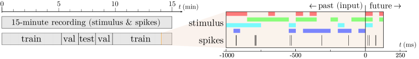
Figure 6: Left: A 15-minute retina recording, split into training, validation and test subsets. Right: A single ~1.1-second snippet taken from the training subset. ${\small t=0}$ separates the snippet into the “past” data, available to the model, and the “future” data, for which models will be expected to make predictions. In our experiments, the length of the past data is always 1 second (992 samples); the length of the future data depends on the model; for example, the Poisson-{5}ms model with a 5-sample summation interval will use 5 samples (~{5}).

6.1 Dataset

Model input was a (5, 992)–shaped array corresponding to 1 second of history: a 4-channel stimulus and a single spike train, both sampled at {992}Hz. The data came from a 15–minute recording of chicken RGCs exposed to full-field colour noise, recorded by Seifert et al. (2023). Appendix A.3 describes this data in more detail. The 15–minute recording was split according to the ratio (7,2,1) into training, validation and test sets. The spike train metrics used for evaluation become less meaningful at low spike counts, so we filtered out cells that contained few spikes in the test set. A minimum threshold of 70 spikes was chosen which resulted in 60 of 154 cells being used. The choice of threshold value was influenced by our computational resources—training time was considered too long for more than 60 cells. Figure 6 gives an overview of the dataset structure. Further details of the dataset are covered in Appendix A.4.

6.2 Models

For each of the 60 cells, 7 models were trained: 1 spike distance model and 6 Poisson models. Each Poisson model used a different summation interval length: 5, 10, 20, 40, 80 and 160 bins. As the duration of 1 bin ({1.0008}) is approximately {1}, these models are referred to as Poisson-{5}, Poisson-{10}, and so on.

A single architecture is not used for both the spike distance objective and the Poisson objective as the former requires output in the form of an array and the latter a scalar; instead, two neural networks are used. These were designed towards maximizing our ability to compare the two learning objectives. An overview of the architectures is shown in Figure 3. The two architectures were designed around a shared base architecture that accounts for the preponderance of parameters and compute. A CNN using ConvNext blocks described by Liu et al. (2022) forms the shared base. The Poisson architecture then ends in a fully-connected layer, whereas the spike distance architecture’s head consists of 4 upsampling ConvNext blocks. There is no weight sharing employed for training on multiple cells—the models are trained end-to-end for each cell individually. The alternative of training on all cells at once by adding per-cell modulation to the network was avoided, as the outputs of the two architectures are very different in nature, and any single modulation scheme may favour one over the other. Further details on the models are described in Appendix A.5.

One concern addressed is layer count. The spike distance architecture has additional layers in its head, and we wished to rule out this difference leading to a performance advantage. This concern was ameliorated by optimizing the number of layers in the shared base architecture to maximize Poisson performance. This architecture search over layer count is described in Appendix A.6.

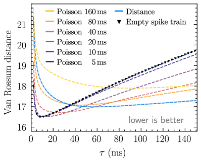
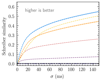
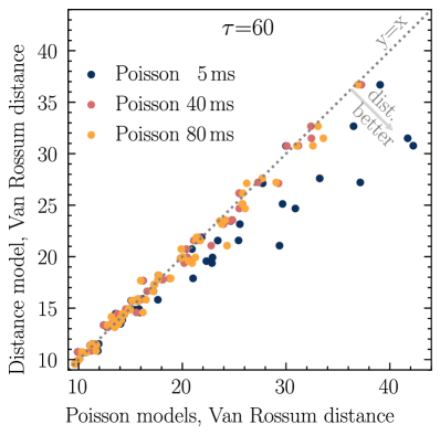
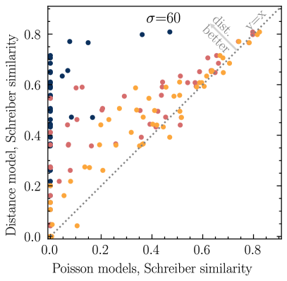
Figure 7: Van Rossum distance (left) and Schreiber similarity (right) between the ground truth spike trains and the model outputs, reported as interquartile mean over the 60 chicken cells. Both metrics are evaluated for a range of their smoothing parameters, $\tau$ and $\sigma$, respectively. 95% confidence intervals are included for the Poisson-{80} and spike distance models. The zero-spike spike train is included for comparison and highlights how the metrics lose their ability to distinguish spike trains at low smoothing levels.

Figure 8: Zoomed in to a single smoothing value from Figure 8, the spike distance model is compared to 3 of the Poisson models for all 60 cells. (left) Van Rossum distance at $\tau=\quantity{60}{ms}$, (right) Schreiber similarity at $\sigma=\quantity{60}{ms}.$

6.3 Training

All models were trained for 80 epochs using the AdamW optimizer with the 1-cycle learning rate policy (Smith, 2017). Loss for the spike distance model was mean squared error between the model output and the log of the target spike distance. Loss for the Poisson models was negative log-likelihood with respect to the target Poisson distribution. The $\lambda$ parameter of the target distribution is the count of spikes within the model’s summation interval. Final models were chosen based on the lowest validation loss across the 80 epochs. Training hyperparameters are described further in Appendix A.7. Total training times are summarized in Appendix A.8.

7 Results

Once trained on a cell, a model was used to infer a spike train using the 90-second test data. Each inferred spike train was compared to the ground truth spike train using three metrics for spike train similarity/dissimilarity: Van Rossum distance (Van Rossum, 2001), Schreiber similarity (Schreiber et al., 2003) and Pearson correlation. Appendix A.2 covers these metrics and the evaluation procedure in more detail.

Training and evaluating a model 60 times, once for each cell, is considered a run. 11 runs were performed for both the spike distance model and the Poisson-{80} model (the most competitive model). All other models were evaluated for a single run. We follow the recommendation of Agarwal et al. (2021) and report aggregate performance for a model using interquartile mean (IQM) across cells and runs; and for the two models with multiple runs, uncertainty is estimated with stratified bootstrap confidence intervals. Model vs. model performance figures are also reported, providing another perspective on the variability across cells.

Van Rossum distance and Schreiber similarity are shown in Figure 8. Figure 8 zooms in on single smoothing parameter for both of these metrics. Pearson correlation is shown in Figure 9 in Appendix A.1. The experiment was repeated under similar conditions for a recording of frog RGCs, and the results for this data are presented in Appendix A.1 also.

8 Discussion

An effective model should perform well over a wide range of smoothing parameters, and in this regard, the spike distance model outperforms the Poisson models in all three metrics. The evaluation settings that least favour the distance model are the Van Rossum distance at low smoothing levels where the short interval Poisson models perform better. In defence of the distance model, it should be noted that the Van Rossum distance acts as a co-incidence detector at low smoothing values, where the absence of spikes is penalized less than the presence of inexact spikes (Paiva et al., 2010, p. 408).

There are several opportunities to improve the performance of the spike distance model: the model architecture can be optimized with the spike distance performance in mind; pretraining part or all of the network using synthetic spike data may improve its ability to produce spike distance arrays; and the real training data can be better utilized by training a single model on multiple cells. Furthermore, the space of algorithms for inferring spikes from spike distance arrays has yet to be explored deeply.

9 Conclusion

We propose using a “distance to spike” representation of a spike train which we call a spike distance function. We show that neural networks can be trained to approximate spike distance functions and that these outputs can be used for spike train inference. For the task of spike prediction, we show that models trained to predict a spike distance function outperform models trained using the standard Poisson objective.

Appendix A Appendix

A.1 Additional results

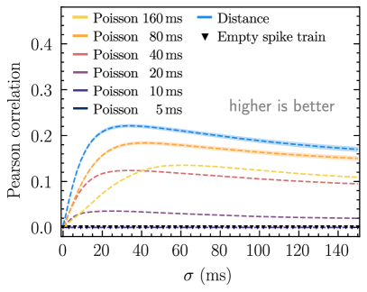
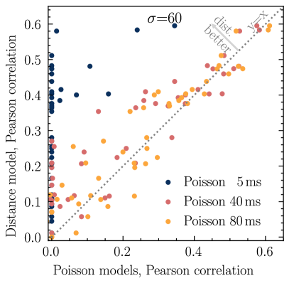
Figure 9: (left) Pearson correlation between the ground truth spike trains and the model outputs, reported as interquartile mean over the 60 chicken cells. Before calculating Pearson correlation, both spike trains are first smoothed with a Gaussian kernel with standard deviation = $\sigma$. 95% confidence intervals are included for the Poisson-{80} and spike distance models. The zero-spike spike train is included for comparison and highlights how the metric loses its ability to distinguish spike trains at low smoothing levels. (right) Zoomed in to a single smoothing value $\sigma=\quantity{60}{ms}$, the spike distance model is compared to 3 of the Poisson models for all 60 cells.

Section 7 results are continued here with Figure 9 reporting Pearson correlation.

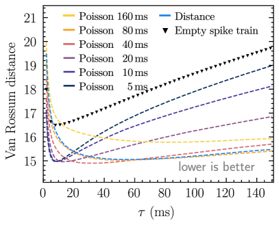
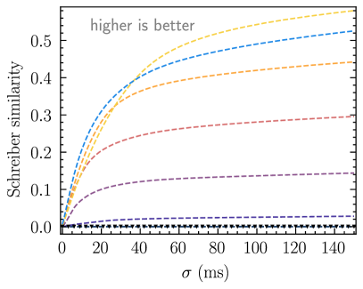
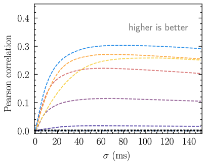
Figure 10: Frog RGCs. (top-left) Van Rossum distance, (top-right) Schreiber similarity and (bottom) Pearson correlation between the ground truth spike trains and the model outputs, reported as interquartile mean over 48 frog cells. All metrics are reported for a range of their smoothing parameters, $\tau$ and $\sigma$. All models are trained for a single run (no confidence intervals). The zero-spike spike train is included for comparison and highlights how the metrics lose their ability to distinguish spike trains at low smoothing levels.

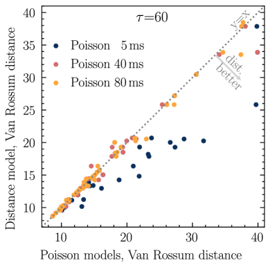
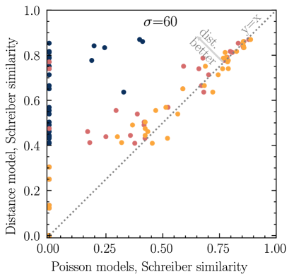
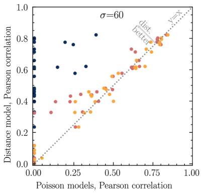
Figure 11: Frog RGCs. Zoomed in to a single smoothing value from Figure 10, the spike distance model is compared to 3 of the Poisson models for all 60 cells. (top-left) Van Rossum distance at $\tau=\quantity{60}{ms}$, (top-right) Schreiber similarity at $\sigma=\quantity{60}{ms}.$, and (bottom) Pearson correlation at $\sigma=\quantity{60}{ms}.$

Xenopus (frog) RGCs were recorded under similar conditions. The same MEAs device was used, and the data preprocessing was mostly the same—a more recently developed (and not yet published, although code is available) quality criterion was used for identifying cells in the recording. Figure 10 shows the Van Rossum distance, Schreiber similarity and Pearson correlation for 48 recorded frog RGCs. Figure 11 gives a model vs. model comparison for these metrics at a fixed smoothing value. All models were trained for a single run only (no confidence intervals). The gap in performance between the spike distance model and the Poisson models is narrower for the frog RGCs in comparison to the chicken RGCs (Figure 8), particularly for Poisson-{80} which is the best-performing model in terms of Van Rossum distance for most $\tau$ smoothing values. Likely contributing to this observation is the putative simplicity of dynamics of frog RGCs in comparison to chicken RGCs [Seifert et al., 2023].

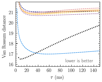
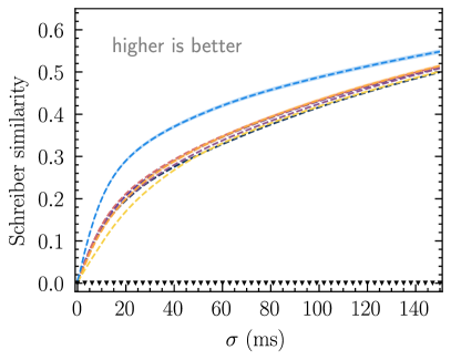
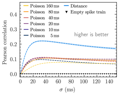
Figure 12: Model comparison when sampling is used for spike prediction with the Poisson models. Van Rossum distance (top-left), Schreiber similarity (top-right) and Pearson correlation (bottom) between the ground truth spike trains and the model outputs, reported as interquartile mean over the 60 chicken cells. All metrics are evaluated for a range of smoothing parameters. 95% confidence intervals are included for the Poisson-{80} and spike distance models. The zero-spike spike train is included for comparison and highlights how the metrics lose their ability to distinguish spike trains at low smoothing levels.

Spike train prediction using a sampling strategy is possible with the Poisson models. The sampling strategy for spike prediction produces quite different results (shown in Figure 12) compared to the maximum likelihood approach. For both Schreiber similarity and Pearson correlation, the performance of the shorter interval Poisson models is rescued, but this comes at the cost of reducing the performance of the better performing models. Poisson-{5} and Poisson-{10} have summation intervals short enough that many outputs are below 0.5, and when using maximum likelihood estimation, these outputs get rounded to 0 to produce a spike count. It is therefore understandable that the performance of these models improve when switching to sampling. In contrast, Poisson-{40}, Poisson-{80} and Poisson-{160} have their more accurate predictions perturbed and see a performance decrease. All models perform far worse according to Van Rossum distance—they perform worse than the empty spike train at all $\tau$ values tested. If one is unable to experiment with various summation intervals, using sampling for prediction can give a higher lower-bound performance across summation intervals compared to the maximum likelihood approach at the cost of incurring a lower peak performance.

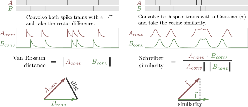
Figure 13: Calculation of Van Rossum distance (left) and Schreiber similarity (right) from two input spike trains. Both metrics employ distinct smoothing kernels to produce an intermediate vector. Van Rossum distance can be thought of as measuring the Euclidean distance between the vectors, while the Schreiber similarity assesses the angle between them.

A.2 Evaluation metrics

In this section, we discuss our choice of evaluation procedure, justifying our choice of metrics, our avoidance of spike binning and our avoidance of stimulus repetitions.

Choosing a spike train metric remains an unsatisfying activity as there is not yet any strong basis on which the characteristics of different metrics can be definitively ranked. We chose Schreiber similarity and Van Rossum distance as they are frequently used, easy to explain, and because each captures a different aspect of spike similarity/difference. Figure 13 describes Van Rossum distance and Schreiber similarity. Pearson correlation is also reported so as to have a common metric with the previous work of McIntosh et al. [2016]. We refer to Paiva et al. [2010] and Sihn and Kim [2019] for a comparison of different spike train measures.

Each of the three spike train metrics used in this work is parameterized by a smoothing parameter. For Van Rossum distance and Schreiber similarity, their parameters are an integral component of their definition. We augment the Pearson correlation by prepending a smoothing step copied from the Schreiber similarity. For Schreiber similarity and Pearson correlation, spike trains are first smoothed with a Gaussian kernel with standard deviation parameter $\sigma$; for Van Rossum distance, the first step is to smooth spike trains with an exponential kernel with decay parameter $\tau$.

Our evaluation departs from previous work by avoiding binning, avoiding fixed smoothing and avoiding multi-trial averaging. In Batty et al. [2016], McIntosh et al. [2016] and Cadena et al. [2019], ground truth spikes are binned then Gaussian smoothed and compared to Gaussian smoothed model outputs. Furthermore, ground truths are averaged over multiple trials in McIntosh et al. [2016] and normalized by the average over multiple trials in Batty et al. [2016] and Cadena et al. [2019]. In each of these studies, the choice of bin size and smoothing filter width were fixed and chosen to match the bin size and smoothing used during training.

As shown in all results, the comparison of spike trains is sensitive to the degree of smoothing, and different models perform best at different smoothing “sweet spots”. There is a scale from instantaneous spikes to temporal averages (rates) over increasing durations. No single point on this scale can capture all that matters about a neuron’s response, so it is important to investigate spiking behaviour over a range of timescales. We evaluate the three metrics at a range of smoothing values: both $\sigma$ and $\tau$ vary from 0 to 150 at integer steps (although below $\tau=2$, Van Rossum distance is large and gets clipped from the figures).

We also eschew averaging or normalizing across repetitions of the same stimulus. As argued by Brette [2015], neuron state is not stable, and differences across stimulus presentations may arise not solely from noise to be disregarded but from the fact that the state of a neuron or network of neurons can change. With this in mind, we present a single stimulus pattern without repetition and delegate the modelling of uncertainty and identification of latent variables to the neural network.

A.3 Retina recording

The main dataset is created from a single 15-minute recording of chicken RGC spike activity carried out by Seifert et al. [2023]. Important aspects of the recording will be summarized here (see Seifert et al. [2023] for full details). A chicken retina was placed on an MEA, and a full-field colour sequence driven by 4-LEDs was projected onto the retina. The colour sequence was a random sequence of 50 ms frames, with each LED having a 50% chance of being on or off in each frame. The electrical activity recorded by the MEA was passed through a spike sorter to produce a sequence of spike events sampled at {17.9}kHz. The stimulus frame changes were also recorded as trigger events at {17.9}kHz. The stimulus was downsampled by a factor of 18 to {992}Hz, and the spike data was rebinned to {992}Hz. Keeping correspondence between the sample period of the stimulus and spike data allows both to be stacked into a single 2D array. Downsampling by 18 was chosen as the sample period of ~{1}ms is short enough that no two spikes are recorded in the same bin, which simplifies the spike distance calculation. Downsampling by 18 is also convenient, as it results in a sample period very close to {1}ms ({1.0008}), enabling number of samples and number of milliseconds to be used interchangeably with little effect on precision. The same proceedure was followed to collect the frog MEA recording.

The spike trains produced by the spike sorter are not a perfect representation of the true spike activity produced by the neurons—false positives, false negatives and the incorrect assignment of spikes to cells are all issues. In this work, we consider the neurons, the multi-electrode array and the spike sorter as a single black box whose behaviour we predict; we do not attempt to make claims about any of the three components individually.

Further processing of the data was carried out in order to create separate training, validation and test sets.

A.4 Dataset

The 15-minute recording was split according to the ratio (7, 2, 1) into training, validation and test sets as shown in Figure 6. As the health of the retina can degrade over the course of the recording altering its behaviour, the (7, 2, 1) split was formed by first splitting the recording by the ratio (7, 2, 2, 2, 7) and then combining segments: the first and last 5.25-minute segments form the training set, the single middle 90-second segment forms the test set, and the two remaining 90-second segments form the validation set. This approach allows the test set to be exposed to both extremes while keeping the test set as a single contiguous chunk.

For the Poisson models, each dataset sample is a tuple (input, target), where the input is a $5\times 992$ array representing 1 second of stimulus and spike history, and the target is a scalar representing the number of spikes in the summation interval. For the spike distance model, each sample is a tuple (input, target) where the input is the same as that for the Poisson models, and the target is a $128$ length array representing ~{128} of ground-truth spike distance data, with $t=0$ positioned at index 32. The choice of these values are hyperparameters discussed in Appendix A.7.

As the dataset’s sequential nature means that adjacent samples will be the same except for a 1 time step shift, we introduce a configurable stride parameter for the training dataset. A larger stride decreases the number of samples that constitute an epoch; this allows model evaluation and checkpoints to be carried out frequently while still being synchronized to epoch completions. The intermediate samples are still used in training, but they appear as augmentations by random indexing between stride indices. For all experiments, the stride was set to 13. A value of 13 resulted in the U-shaped learning curve being observed over 80 epochs.

Layer	Input size	Kernels (length, channels, stride)	Output size
Initial conv	5$\times$992	$\begin{bmatrix}15,&64,&2\end{bmatrix}\times 1$	$64\times 496$
ConvNext blocks (downsampling)	64 $\times$ 496	$\begin{bmatrix}3&64&2\\ 1&128&1\\ 5&128&1\\ 1&64&1\end{bmatrix}$ $\times$ 6	$64\times 8$
ConvNext blocks	$64\times 8$	$\begin{bmatrix}1,&128,&1\\ 3,&128,&1\\ 1,&64,&1\end{bmatrix}\times 4$	$64\times 8$

Table 1: Base architecture shared by both Poisson and spike distance models. ~{302} parameters, ~{8.28} multi-adds.

Layer	Input size	Kernels (length, channels, stride)	Output size
ConvNext	64 $\times$ 8	$\begin{bmatrix}1,&128,&1\\ 5,&128,&1\\ 1,&16,&1\end{bmatrix}\times 1$	16 $\times$ 16
ConvNext	$16\times 16$	$\begin{bmatrix}1,&32,&1\\ 5,&32,&1\\ 1,&16,&1\end{bmatrix}\times 3$	$16\times 128$
Conv	$16\times 128$	$\begin{bmatrix}1,&1,&1\end{bmatrix}\times 1$	$1\times 128$

Table 2: Distance model head. ~{29} parameters, ~{587} multi-adds.

Layer	Input size	Kernels (length, channels, stride)	Output size
Flatten	$64\times 8$	None	512
FC layer	$512\times 1$	$\begin{bmatrix}1,&512,&1\end{bmatrix}$	1

Table 3: Poisson model head. 513 parameters, 513 multi-adds.

A.5 Models

The convolutional kernels used in the shared base architecture are shown in Table A.4. In addition to the convolutional layers, a learnable positional embedding was added to the output of the initial convolutional layer of the shared architecture. The kernels used for the spike distance head and the Poisson head are shown in Table 2 and 3 respectively. The shared base architecture accounts for 88% of parameters and 93% of multi-adds in the spike distance model, and accounts for practically all the parameters and multi-adds for the Poisson models.

ConvNext blocks introduced by Liu et al. [2022] were chosen to form the main component of the architecture as they are commonly used and well-tested. Our implementation includes the Global Response Normalization layer (GRN) from ConvNextv2 blocks introduced by Woo et al. [2023]. We use dropout at the end of each block, at a rate of 0.2.

A.6 Architecture search

The number of mid-layers in the shared base architecture was varied in order to increase confidence that performance differences between the spike distance model and the Poisson models are not due to differences in layer and parameter counts. The number of mid-layers was varied between 0 and 7 (inclusive) and the configuration that best served the Poisson-{80} model was chosen. This selection was based on the interquartile mean of the loss across cells in the validation set. Focus was given to the Poisson-{80} model as it was observed to be the most competitive Poisson model.

For each of these configurations, the Poisson-{80} model was trained once for each of the 60 chicken RGCs. The interquartile mean loss is shown in Figure 15. To gauge the magnitude of the effect on metrics, the interquartile mean Pearson correlation is reported in Figure 15. Other metrics show a similar lack of dependency on layer count. The 5-layer configuration was selected based on the loss; however, it seems like the number of mid-layers has very little effect on the performance of the Poisson-{80} model.

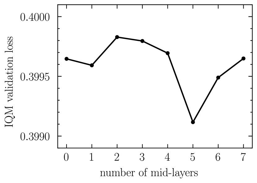
Figure 14: Interquartile mean validation loss for a range of mid-layer counts. The IQM is calculated over the 60 separately trained Poisson-80 models, one for each of the 60 RGCs. The loss is the mean validation set loss.

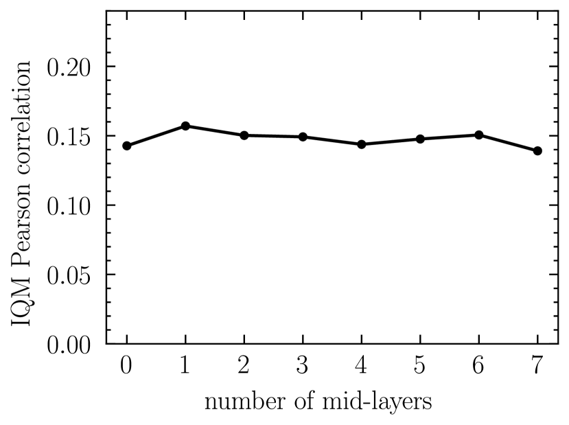
Figure 15: Interquartile mean Pearson correlation for a range of mid-layer counts. The IQM is calculated over the 60 separately trained Poisson-80 models, one for each of the 60 RGCs. Pearson correlation is calculated between the output and validation set ground-truth spike trains, smoothed with a Gaussian kernel with $\sigma=20$.

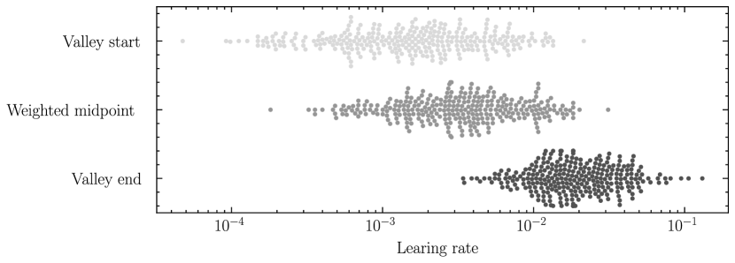
Figure 16: Three learning rates identified by the range test for learning rates described by Smith and Topin [2019]. Valley start and valley end describe the edges of the U-shaped valley containing the suggested learning rate, which is a weighting of the edges.

A.7 Hyperparameters

A list of hyperparameters associated with models, training and inference.

Architecture. The following settings are associated with the model architectures.

• Channel count in the shared base: 64. Early experiments not reported here found 32 to have slightly worse performance for all models, and 64 and 128 were observed to have similar performance.

• Channel count in the distance model head: 16. Increasing this setting was observed to increase performance; however, to keep the model’s parameter count close to that of the Poisson models, the channel count was kept low.

• Channel expansion factor of the ConvNext blocks: 2. Changes to this value were not tested.

• Dropout rate: 0.2. Early experiments not reported here observed benefits of dropout for all models. Once added, the dropout rate was not experimented with further.

Training. Settings associated with training were chosen as described below.

• Maximum learning rate: $5\text{\times}{10}^{-4}$. This was chosen by running the LR range test introduced by Smith and Topin [2019] on an earlier architecture for all chicken RGCs. After finalizing the architecture (see Appendix A.6), the range test was run again to ensure that the learning rate was still appropriate. Figure 16 plots the results of this second range test, which supports $5\times 10^{-4}$ still being an appropriate learning rate.

• Batch size: 256. Smaller batch sizes resulted in a training speed considered onerously slow.

• Dataset stride: 13. The dataset stride is described in Appendix A.4.

• Epochs: 80. Training is carried out for 80 epochs. Each time step will be part of a model input on average $80\times\frac{992}{13}=6105$ times.

• AdamW parameters: $(\beta_{1},\beta_{2},\text{eps},\text{weight decay})=(0.9,0.99,$1\text{\times}{10}^{-5}$,0.3)$. These were chosen in line with heuristics described by Howard et al. [2020].

• Learning rate scheduler: 1-cycle scheduler policy described by Smith and Topin [2019] was used, with three-phase enabled and other options as default values in Pytorch 2.0’s implementation.

• Precision: Nvidia’s automatic mixed precision was used.

Spike distance. A number of settings were used to control the nature of the output spike distance array and the inference process:

• stride: how many time steps to shift forward when carrying out autoregressive inference. This was set to 80 time steps (~{80}ms). Shorter strides offer improved inference at the cost of increased compute. 80 was chosen to match the Poisson-{80} model.

• $L$: the length of the spike distance array the model outputs. 128 is the next power of two greater than 80, allowing the distance model’s head to be a simple sequence of 4 upsample blocks. The additional time steps were split between before $t=0$ and after $t=\quantity{80}{ms}$ according to the next setting, $i_{0}$.

• $i_{o}$: the index into the array that corresponds to $t=0$. This was set to 32. A low value negatively affects inference as described in Appendix A.9.2. 32 was chosen as it is the length of 2 activations before passing through the 4 upsample blocks (leaving 1 activation that extends past t=80). A search for an optimal value has not been carried out.

• $M$: the maximum distance for an element of the spike distance field. This was set to {200}ms. This is not a very sensitive parameter. A few settings were experimented with, as described in Appendix A.9.1.

A.8 Computational resources

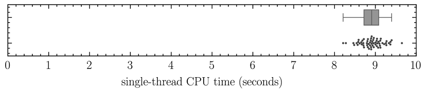
Figure 17: Running time of Algorithm 1 to infer 90-seconds of spike behaviour for 60 cells, in steps of {80}. Running time is calculated with Python’s timeit package. In order to isolate the running time of Algorithm 1, inference is not autoregressive, and instead uses precalculated model outputs as inputs to the algorithm. (Mean, standard deviation) = (8.9, 0.27).

All training and inference was carried out on a single workstation, with CPU, GPU and RAM specifications: AMD Ryzen 9 5900X CPU, Nvidia RTX 3090 GPU and 128 GiB RAM.

Training a single model on all 60 chicken RGCs took ~{12}hours. This was repeated 11 times for the Poisson-{80}ms model and the spike distance model in order to calculate confidence intervals. Only 1 repeat was carried out for the remaining five Poisson models. For architecture variations, the Poisson-{80} model was trained 8 times for all RGCs to investigate the number of mid-layers. Training on the frog RGCs took ~{10}hours, and was done once for each of the 7 models.

The total training time was ~{490}hours:

$$(\quantity{12}{hours\per model}\times\quantity[parse-numbers=false]{(2\times 11+5+8)}{models}+\quantity{10}{hours\per model}\times\quantity{7}{models})=490.$$

Inference was considerably quicker, taking a total of ~7 hours summed over all experiments.

A.9 Spike distance

This section covers some details on working with spike distance: choosing a maximum spike distance, and the benefits to inference of outputting an extended spike distance.

A.9.1 Maximum spike distance

If there are no spikes, then the distance to the nearest spike can be considered infinite. When approximating a distance function, infinite distances can be avoided by fixing a maximum allowed distance. The choice of a maximum is important beyond simply the avoidance of undefined values—it is also useful to limit how far into the past or future we expect a distance function to be reasonably approximated. Consider the spike distance function $f_{S}$ evaluated at some time point $t_{1}$. The single value $f_{S}(t_{1})$ contains information about all time points in the interval $[t_{1}-f_{S}(t_{1}),t_{1}+f_{S}(t_{1})]$. For example, if $f_{S}(t_{1})=10$, then we know that there are no spikes in the open interval $(t_{1}-10,t_{1}+10)$. When training a model for spike prediction, we don’t expect the model to anticipate spiking activity far into the future. For a model that predicts spike distance, one way to limit its exposure to the future is to clamp the target spike distance function. In this paper, we work with a maximum spike distance of {200}ms. Through experimentation not reported here, for the dataset used in this paper, we tested a range of maximum distances and found that there was not a major difference in performance when the maximum spike distance is between {100}ms and {600}ms. Below {100}ms and above {600}ms performance begins to degrade.

A.9.2 An extended spike distance improves inference

Spike prediction performance is improved if the spike distance function outputted by the neural network extends both before and after the interval in which spikes are to be predicted. This means that when predicting $L$ time steps starting from $t_{0}$, the neural network should output a spike distance function that extends both before $t_{0}$ and after $t_{0}+L$.

The reason for this lies in the capacity of spike distance to carry information about a spike train both before and after the time point at which it is evaluated. For example, the spike distance at $t_{0}-1$ (past) can be affected by spikes that come after $t_{0}$ (future). In other words, the spike distance representation for a spike train does not fall neatly into the same time interval. By extending the spike distance function before $t_{0}$ and after $t_{0}+L$, there is more information available for the inference algorithm to judge the placement of spikes. The model presented in this work is trained to output a spike distance array of length $128$, where $32$ elements are assigned to the past. If predicting a spike train for 80 time steps into the future, then there would be $16$ elements of the model’s output remaining that extend beyond the end of the spike train.

A.10 Discrete spike distance

In practice, both spike times and spike distance will be discretized. Instead of the input being exact spike times, we will use spike counts sampled at a certain sample period $T$, and instead of evaluating the spike distance at any real, we will evaluate the distance at discrete times separated by the same period $T$ and collect the values in a spike distance array.

A naive and computationally simple approach of approximating the continuous spike distance is to count the number of samples until a sample with a non-zero spike count. This is a suitable approach when the sample rate is fast in comparison to the spike rate and spikes are rarely coincident in the same sample. Indeed, the main results in this work involve sample frequencies fast enough that no spikes are coincident in the same sample. When using a slower sampling rate, it may be beneficial to use the approach outlined below, which more faithfully discretizes the minimum distance when there is uncertainty over the precise location spikes.

To approximate the continuous spike distance function $f_{S}(t):\mathbb{R}\to\mathbb{R}$ introduced in Section 4, we are seeking a function $\hat{f}_{S}(t):\mathbb{N}\to\mathbb{R}$ that is a faithful approximation when both spike times and the points being evaluated are discretized. Osher and Fedkiw [2003] presents several methods for discretizing implicit representations; there the authors use known properties of the physical systems being modelled in order to discretize implicit functions. Our spike events are far less analytically constrained, and so we will instead take a probabilistic approach.

A.10.1 Motivating the discrete spike distance

In the continuous case, the two points between which a distance is calculated are obvious: the spike time and the time for which the spike distance is being evaluated. In the discrete case, we must consider candidates for both of these time points.

Consider recording spikes at a sample period $T=\quantity{20}{ms}$, where each sample is a sum of the spikes that occurred within a $\quantity{20}{ms}$ interval. If a single spike is recorded in the 5^th sample, and the 5^th sample collected spikes from the interval $(\quantity{80}{ms},\quantity{100}{ms})$, then where in this interval should consider the spike to have occurred? Another question: if we wish to calculate an array of spike distances at some sample rate, what reference point should each sample use from which to measure distance? For spike times there is uncertainty, and for reference points there is a choice to be made.

A few decisions and assumptions are enough to determine a discrete distance. First, we will treat spike times as being random variables distributed uniformly over the sample in which they are recorded. This decision is reasonable when the samples represent a count of spikes within an interval, and there is no further information about the location of spikes within the interval. Indeed, this is the case for this work—the spike events are outputs of a black-box detection mechanism of the MEA and are subsequently rebinned to reduce the sample rate. The second decision is to fix our array of distance calculations to the same frequency as the spike recording, and we measure distances from the midpoint of each interval.

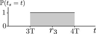
Figure 18: If one spike is detected in sample 3, then the spike distance for sample 3 is given by $\hat{f}(3)=\mathbb{E}[t_{3}-r_{3}]=0.25T$, where $r_{3}=3.5T$ and $t_{3}$ is a random variable uniformly distributed over $[3T,4T]$.

To appreciate the implications of these choices, consider the case where a single spike is recorded in sample $i$ and we wish to evaluate the discrete spike distance for the same index, $i$. The naive solution is to define $\hat{f}_{S}(i)=0$. However, 0 is not a good representation of the spike distance over the whole interval $[iT,(i+1)T]$; 0 is only ever the value of the spike distance at the instantaneous time a spike occurs. A better value for $\hat{f}_{S}(i)$ should incorporate the fact that there is uncertainty about when exactly a spike occurs within this interval of length T. The approach we take goes as follows. Fix the reference point $r_{s}$ from which spike distances are measured to be the interval’s midpoint, $r_{s}=(i+0.5)T$. Consider the spike time to have a uniform distribution over the interval $[iT,(i+1)T]$. The value for $\hat{f}_{S}(i)$ will be defined as the expected distance to the reference point, where the expectation is calculated over the uniformly distributed spike time. Figure 18 shows this case in more detail. The next section formalizes these ideas and arrives at a simple procedure for calculating the discrete spike distance from a sequence of spike counts.

A.10.2 Definition and calculation

What follows is a formalization of the discrete spike distance that can be thought of as applying extreme value theory to spike distances. Coles [2001] is a good introduction to extreme value statistics. What prevents the direct use of a plug-and-play theorem from extreme value theory is that in our situation we are not interested in the asymptotic behaviour of an unknown distribution, but the finite behaviour of a known distribution.

Set the scene with two definitions. Similar to how the continuous spike distance function was parameterized by a set of spike times, the discrete spike distance function is parameterized by a sequence of spike counts.

Definition 1.

Let $T\in\mathbb{R}$ be the sample rate. Let $l\in\mathbb{N}$ be a positive integer representing the number of samples. Then a spike count sequence $S=(s_{i})_{i=0}^{l-1}$ at sample rate $T$ is a sequence of spike counts, where $s_{i}$ is the number of spikes recorded in the interval $[iT,(i+1)T]$.

If $S=(s_{i})_{i=0}^{l-1}$ is a spike count sequence with a total spike count $n=\sum_{i=0}^{l-1}s_{i}$, we can associate with it a sequence of independent random variables, $X_{0},X_{1},\ldots X_{n-1}$, where each $X_{j}$ represents a spike time distributed uniformly over one of the length $T$ intervals. For example, if $s_{0}=3$ and $s_{1}=1$, then $X_{0},X_{1}$ and $X_{2}$ would be distributed uniformly over the interval $[0,T]$ while $X_{3}$ would be uniformly distributed over the interval $[T,2T]$.

Definition 2.

Let $i$ be a sample index. Let $S$ be a spike count sequence and let $X_{0},X_{1},...X_{n-1}$ be independently identically distributed real random variables representing the spike times of the $n$ spikes from $S$. Each $X_{j}$ is distributed uniformly over the sample interval in which it is recorded. Let $r_{i}=i+0.5$ represent the midpoint of the $i^{\text{th}}$ sample interval. For each $X_{j}$ let $D_{j}=|X_{j}-r_{i}|$ be the derived random variable representing the distance of the $j^{\text{th}}$ spike to the midpoint $r_{i}$. The discrete spike distance function $\hat{f}_{S}:\mathbb{N}\to\mathbb{R}$ at $i$ is given by:

$$\hat{f}_{S}(i)=\mathbb{E}_{D_{0},D_{1},\ldots,D_{n-1}}\min_{0\leq j<n}\;D_{j}\;$$ (2)

and has units of the sampling period, $T$.

Calculating this value involves considering only the one or two samples containing spikes that are closest to the sample of interest, $i$. This could be sample $i$ itself, a single sample to the left or right of $i$ or two samples equidistant to $i$, one of either side. Being able to ignore most of the samples allows for the discrete spike distance to be expressed neatly in terms of the spike counts of the closest non-empty sample(s).

Proposition 3.

Let $d\in\mathbb{N}$ be the difference in samples between the sample of interest $i$ and the closest spike-containing sample(s). Let $m\in\mathbb{N}$ the number of spikes contained within the closest spike-containing sample(s).

The value of $\hat{f}_{S}(i)$ from Equation 2 is given by:

$$\hat{f}_{S}(i)=\begin{cases}\hat{f}_{S}(i)=\frac{1}{2(m+1)}&\text{there are one or more spikes in sample }i\vspace{6pt}\\ \hat{f}_{S}(i)=d-\frac{1}{2}+\frac{1}{m+1}&\text{otherwise.}\end{cases}$$ (3)

Proof.

First, the first case: there are $m>0$ spikes in sample $i$. The presence of the $\min$ function in Equation 2 means that we can ignore all spikes that are not in sample $i$, as they will not affect the expectation. Let $D_{0},D_{1},...D_{m-1}$ be the random variables representing the distance of the $m^{th}$ spike recorded within sample $i$. Single out one of these, $D_{1}$, and we will return later to include the others. $D_{1}$ will contribute to the expectation only when it is smaller than all others: if $D_{1}=t$, then all $m-1$ other distances must be greater than $t$. The probability $\mathbb{P}(D_{1}=t)=2$ (uniform over interval of length $\frac{1}{2}$) and the probability of other $D_{j}$ having a value larger than $t$ is $\mathbb{P}(D_{j}>t)=2(\frac{1}{2}-t)$.

The contribution to the expectation for $D_{1}$ then amounts to:

$$\int_{0}^{\frac{1}{2}}t\cdot\mathbb{P}(D_{1}=t)\prod_{j=1}^{m-1}\mathbb{P}(D_{j}>t)\differential{t} =\int_{0}^{\frac{1}{2}}t\cdot(2)\prod_{j=1}^{m-1}(2)(\frac{1}{2}-t)\differential{t}$$

$$=2\int_{0}^{\frac{1}{2}}t(1-2t)^{m-1}\differential{t}$$

$$=2\left[-\frac{t}{m}(1-2t)^{m}\right]_{0}^{\frac{1}{2}}+\int_{0}^{\frac{1}{2}}\frac{1}{m}(1-2t)^{m}\differential{t}$$

$$=0+\left[-\frac{1}{2m(m+1)}(1-2t)^{m+1}\right]_{0}^{\frac{1}{2}}$$

$$=\frac{1}{2m(m+1)}\;.$$

We singled out $D_{1}$; however, any of the $m$ spikes are equally likely to be the closest spike. Summing the contribution over $m$ spikes gives us:

$$\frac{1}{2(m+1)}$$

as required by the first case.

What distinguished the second case is that the reference point $r_{i}$ is not in the same sample as the closest spike(s). Let $m>0$ be the number of spikes that are in the closest one or two samples, situated $d$ samples from the sample of interest $i$. We ignore all other spikes. Let $D_{0},D_{1},...D_{m-1}$ be the random variables representing the distance of the $m^{th}$ spike to the reference point $r_{i}$. Single out one of these, $D_{1}$. $D_{1}$ will contribute to the expectation only when it is smaller than all others: if $D_{1}=t$, then all $m-1$ other distances must be greater than $t$. This time, $D_{1}$ has a uniform distribution over the interval $[d-\frac{1}{2},d+\frac{1}{2}]$ of length $1$ with $\mathbb{P}(D_{1}=t)=1$ in this interval. The probability of other $D_{j}$ having a value larger than $t$ is $\mathbb{P}(D_{j}>t)=d+\frac{1}{2}-t$.

The contribution to the expectation for $D_{1}$ then amounts to:

$$\int_{d-\frac{1}{2}}^{d+\frac{1}{2}}t\cdot\mathbb{P}(D_{1}=t)\prod_{j=1}^{m-1}\mathbb{P}(D_{j}>t)\differential{t}$$

$$=\int_{d-\frac{1}{2}}^{d+\frac{1}{2}}t\cdot(1)\prod_{j=1}^{m-1}(d+\frac{1}{2}-t)\differential{t}$$

$$=\int_{0}^{1}(d-\frac{1}{2}+t)\cdot(1)\prod_{j=1}^{m-1}(1-t)\differential{t} (\text{change of variable})$$

$$=\int_{0}^{1}(d-\frac{1}{2}+t)(1-t)^{m-1}\differential{t}$$

$$=\left[-\frac{d-\frac{1}{2}+t}{m}(1-t)^{m}\right]_{0}^{1}+\int_{0}^{1}\frac{1}{m}(1-t)^{m}\differential{t}$$

$$=\frac{d-\frac{1}{2}}{m}+\left[-\frac{1}{m(m+1)}(1-t)^{m+1}\right]_{0}^{1}$$

$$=\frac{d-\frac{1}{2}}{m}+\frac{1}{m(m+1)}\;.$$

We singled out $D_{1}$; however, any of the $m$ spikes are equally likely to be the closest spike. Summing the contribution over $m$ spikes gives us:

$$d-\frac{1}{2}+\frac{1}{m(m+1)}$$

as required by the second case. $\square$

Table 4 compares the discrete spike distance described above to the approximate spike distance, including the values for $m$ and $d$ from Equation 3.

sample index, $i$	$0$	$1$	$2$	$3$	$4$	$5$	$6$	$7$	$8$
spikes			$|$						$||$
$m$	$1$	$1$	$1$	$1$	$1$	$3$	$2$	$2$	$2$
$d$	2	1	$0$	1	2	3	2	1	$0$
spike distance, $\hat{f}_{S}(i)$, in units of $T$	$2$	$1$	$\frac{1}{4}$	$1$	$2$	$2\frac{3}{4}$	$1\frac{5}{6}$	$\frac{5}{6}$	$\frac{1}{6}$
approx. spike distance, in units of $T$	$2$	$1$	$0$	$1$	$2$	$3$	$2$	$1$	$0$

Table 4: The approximate spike distance compared to the discrete spike distance. Discrete spike distances are evaluated for the samples 0 to 8 when there are three spikes recorded: one in sample $2$ and two in sample $8$.

A.11 Open-source implementation and data

The chicken and frog data, along with the code used for training and evaluation is available at https://github.com/kevindoran/spikedistance.

References

- Agarwal et al. [2021] Rishabh Agarwal, Max Schwarzer, Pablo Samuel Castro, Aaron C Courville, and Marc Bellemare. Deep Reinforcement Learning at the Edge of the Statistical Precipice. In Advances in Neural Information Processing Systems, volume 34, pages 29304–29320. Curran Associates, Inc., 2021.
- Batty et al. [2016] Eleanor Batty, Josh Merel, Nora Brackbill, Alexander Heitman, Alexander Sher, Alan Litke, E. J. Chichilnisky, and Liam Paninski. Multilayer Recurrent Network Models of Primate Retinal Ganglion Cell Responses. In International Conference on Learning Representations, November 2016.
- Berry and Meister [1998] Michael J. Berry and Markus Meister. Refractoriness and Neural Precision. Journal of Neuroscience, 18(6):2200–2211, March 1998. ISSN 0270-6474, 1529-2401. doi: 10.1523/JNEUROSCI.18-06-02200.1998.
- Berry et al. [1997] Michael J. Berry, David K. Warland, and Markus Meister. The structure and precision of retinal spike trains. Proceedings of the National Academy of Sciences, 94(10):5411–5416, May 1997. doi: 10.1073/pnas.94.10.5411.
- Brette [2015] Romain Brette. Philosophy of the Spike: Rate-Based vs. Spike-Based Theories of the Brain. Frontiers in Systems Neuroscience, 9, 2015. ISSN 1662-5137.
- Butts et al. [2011] Daniel A. Butts, Chong Weng, Jianzhong Jin, Jose-Manuel Alonso, and Liam Paninski. Temporal precision in the visual pathway through the interplay of excitation and stimulus-driven suppression. The Journal of Neuroscience: The Official Journal of the Society for Neuroscience, 31(31):11313–11327, August 2011. ISSN 1529-2401. doi: 10.1523/JNEUROSCI.0434-11.2011.
- Cadena et al. [2019] Santiago A. Cadena, George H. Denfield, Edgar Y. Walker, Leon A. Gatys, Andreas S. Tolias, Matthias Bethge, and Alexander S. Ecker. Deep convolutional models improve predictions of macaque V1 responses to natural images. PLOS Computational Biology, 15(4):1–27, April 2019. doi: 10.1371/journal.pcbi.1006897.
- Coles [2001] Stuart Coles. An Introduction to Statistical Modeling of Extreme Values. Springer Series in Statistics. Springer, London, 2001. ISBN 978-1-84996-874-4 978-1-4471-3675-0. doi: 10.1007/978-1-4471-3675-0.
- Dai et al. [2017] Angela Dai, Charles Ruizhongtai Qi, and Matthias Nießner. Shape Completion using 3D-Encoder-Predictor CNNs and Shape Synthesis, April 2017.
- Howard et al. [2020] Jeremy Howard, Sylvain Gugger, and Soumith Chintala. Deep Learning for Coders with Fastai and PyTorch: AI Applications without a PhD. O’Reilly Media, Inc, Sebastopol, California, first edition edition, 2020. ISBN 978-1-4920-4552-6.
- Keat et al. [2001] Justin Keat, Pamela Reinagel, R. Clay Reid, and Markus Meister. Predicting Every Spike: A Model for the Responses of Visual Neurons. Neuron, 30(3):803–817, May 2001. ISSN 0896-6273. doi: 10.1016/S0896-6273(01)00322-1.
- Liu et al. [2022] Zhuang Liu, Hanzi Mao, Chao-Yuan Wu, Christoph Feichtenhofer, Trevor Darrell, and Saining Xie. A ConvNet for the 2020s. In 2022 IEEE/CVF Conference on Computer Vision and Pattern Recognition (CVPR), pages 11966–11976, June 2022. doi: 10.1109/CVPR52688.2022.01167.
- McIntosh et al. [2016] Lane McIntosh, Niru Maheswaranathan, Aran Nayebi, Surya Ganguli, and Stephen Baccus. Deep Learning Models of the Retinal Response to Natural Scenes. In Advances in Neural Information Processing Systems, volume 29. Curran Associates, Inc., 2016.
- Osher and Fedkiw [2003] Stanley Osher and Ronald Fedkiw. Level Set Methods and Dynamic Implicit Surfaces, volume 153 of Applied Mathematical Sciences. Springer, New York, NY, 2003. ISBN 978-1-4684-9251-4 978-0-387-22746-7. doi: 10.1007/b98879.
- Paiva et al. [2010] Antonio R. C. Paiva, Il Memming Park, and Jose C. Principe. A comparison of binless spike train measures. Neural Computing and Applications, 19(3):405–419, April 2010. doi: 10.1007/s00521-009-0307-6.
- Park et al. [2019] Jeong Joon Park, Peter Florence, Julian Straub, Richard Newcombe, and Steven Lovegrove. DeepSDF: Learning Continuous Signed Distance Functions for Shape Representation. In 2019 IEEE/CVF Conference on Computer Vision and Pattern Recognition (CVPR), pages 165–174, June 2019. doi: 10.1109/CVPR.2019.00025.
- Ren et al. [2020] Christopher X. Ren, Claudia Hulbert, Paul A. Johnson, and Bertrand Rouet-Leduc. Chapter Two - Machine learning and fault rupture: A review. In Ben Moseley and Lion Krischer, editors, Advances in Geophysics, volume 61 of Machine Learning in Geosciences, pages 57–107. Elsevier, January 2020. doi: 10.1016/bs.agph.2020.08.003.
- Rouet-Leduc et al. [2017] Bertrand Rouet-Leduc, Claudia Hulbert, Nicholas Lubbers, Kipton Barros, Colin J. Humphreys, and Paul A. Johnson. Machine Learning Predicts Laboratory Earthquakes. Geophysical Research Letters, 44(18):9276–9282, 2017. ISSN 1944-8007. doi: 10.1002/2017GL074677.
- Schreiber et al. [2003] Susanne Schreiber, Susanne Schreiber, Jean Marc Fellous, Diane Whitmer, Paul H. E. Tiesinga, and Terrence J. Sejnowski. A new correlation-based measure of spike timing reliability. Neurocomputing, 52:925–931, June 2003. doi: 10.1016/s0925-2312(02)00838-x.
- Seifert et al. [2023] Marvin Seifert, Paul A. Roberts, George Kafetzis, Daniel Osorio, and Tom Baden. Birds multiplex spectral and temporal visual information via retinal On- and Off-channels. Nature Communications, 14(1):5308, August 2023. ISSN 2041-1723. doi: 10.1038/s41467-023-41032-z.
- Sihn and Kim [2019] Duho Sihn and Sung-Phil Kim. A Spike Train Distance Robust to Firing Rate Changes Based on the Earth Mover’s Distance. Frontiers in Computational Neuroscience, 13:82–82, January 2019. doi: 10.3389/fncom.2019.00082.
- Sitzmann et al. [2021] Vincent Sitzmann, Semon Rezchikov, Bill Freeman, Josh Tenenbaum, and Fredo Durand. Light Field Networks: Neural Scene Representations with Single-Evaluation Rendering. In Advances in Neural Information Processing Systems, volume 34, pages 19313–19325. Curran Associates, Inc., 2021.
- Smith [2017] Leslie N. Smith. Cyclical Learning Rates for Training Neural Networks. In 2017 IEEE Winter Conference on Applications of Computer Vision (WACV), pages 464–472, March 2017. doi: 10.1109/WACV.2017.58.
- Smith and Topin [2019] Leslie N. Smith and Nicholay Topin. Super-convergence: Very fast training of neural networks using large learning rates. In Tien Pham, editor, Artificial Intelligence and Machine Learning for Multi-Domain Operations Applications, page 36, Baltimore, United States, May 2019. SPIE. ISBN 978-1-5106-2677-5 978-1-5106-2678-2. doi: 10.1117/12.2520589.
- Uzzell and Chichilnisky [2004] V. J. Uzzell and E. J. Chichilnisky. Precision of Spike Trains in Primate Retinal Ganglion Cells. Journal of Neurophysiology, 92(2):780–789, August 2004. ISSN 0022-3077. doi: 10.1152/jn.01171.2003.
- Van Rossum [2001] M. C. W. Van Rossum. A Novel Spike Distance. Neural Computation, 13(4):751–763, April 2001. doi: 10.1162/089976601300014321.
- Wang et al. [2022] Kun Wang, Christopher W. Johnson, Kane C. Bennett, and Paul A. Johnson. Predicting Future Laboratory Fault Friction Through Deep Learning Transformer Models. Geophysical Research Letters, 49(19):e2022GL098233, October 2022. ISSN 0094-8276, 1944-8007. doi: 10.1029/2022GL098233.
- Weber and Pillow [2017] Alison I. Weber and Jonathan W. Pillow. Capturing the Dynamical Repertoire of Single Neurons with Generalized Linear Models. Neural Computation, 29(12):3260–3289, December 2017. ISSN 0899-7667. doi: 10.1162/neco_a_01021.
- Woo et al. [2023] Sanghyun Woo, Shoubhik Debnath, Ronghang Hu, Xinlei Chen, Zhuang Liu, In So Kweon, and Saining Xie. ConvNeXt V2: Co-Designing and Scaling ConvNets With Masked Autoencoders. In Proceedings of the IEEE/CVF Conference on Computer Vision and Pattern Recognition, pages 16133–16142, 2023.
- Zeng et al. [2017] Andy Zeng, Shuran Song, Matthias Nießner, Matthew Fisher, Jianxiong Xiao, and Thomas Funkhouser. 3DMatch: Learning Local Geometric Descriptors from RGB-D Reconstructions. In 2017 IEEE Conference on Computer Vision and Pattern Recognition (CVPR), pages 199–208, July 2017. doi: 10.1109/CVPR.2017.29.