Optimal Phase Estimation in Finite-dimensional Fock Space

Abstract

Phase estimation is a major mission in quantum metrology. In the finite-dimensional Fock space the NOON state ceases to be optimal when the particle number is fixed yet not equal to the space dimension minus one, and what is the true optimal state in this case is still undiscovered. Hereby we present three theorems to answer this question and provide a complete optimal scheme to realize the ultimate precision limit in practice. These optimal states reveal an important fact that the space dimension could be treated as a metrological resource, and the given scheme is particularly useful in scenarios where weak light or limited particle number is demanded.

As a fundamental scenario, phase estimation is undoubtedly a core topic in precision measurement. Many measurement scenarios, such as ranging, can be naturally translated or modeled into the problem of phase estimation. In quantum mechanics, optical quantum phase estimation is the first scenario revealing the power of quantum resources to beat the standard quantum limit, thanks to the pioneer works of Caves [1, 2]. After decades of studies, quantum phase estimation has now become one of the most fertile fields in quantum metrology [3, 4, 5, 6, 7, 8, 9, 10, 11, 12, 13, 14, 15, 16, 17, 18, 19, 20, 21, 22, 23, 24, 25, 26], and many useful schemes have already been experimentally realized [28, 29, 27, 30, 31, 32, 33, 34, 35, 36].

In quantum phase estimation, especially optical phase estimation, both linear and nonlinear phase shifts can be used to encode the phase. In theory, the linear phase accumulation on a bosonic mode $a$ can be described by the operator $\exp(i\phi_{a}a^{{\dagger}}a)$ with $\phi_{a}$ the accumulated phase. For two modes ($a$ and $b$) with such processes, the total phase accumulations can also be written as $\exp(i\phi_{\mathrm{tot}}n/2)\exp(i\phi J_{z})$ with $\phi_{\mathrm{tot}}=\phi_{a}+\phi_{b}$ the total phase and $\phi=\phi_{a}-\phi_{b}$ the phase difference. $n=a^{{\dagger}}a+b^{{\dagger}}b$ is the operator for the average total photon number and $J_{z}=(a^{{\dagger}}a-b^{{\dagger}}b)/2$ is a Schwinger operator. Similarly, the nonlinear phase accumulation on mode $a$ can be described by $\exp(i\phi_{a}(a^{{\dagger}}a)^{2})$ and for two bosonic modes it becomes $\exp(i\phi_{\mathrm{tot}}[(a^{{\dagger}}a)^{2}+(b^{{\dagger}}b)^{2}]/2)\exp(i\phi nJ_{z})$. In this paper both linear and nonlinear phase shifts will be studied and the phase difference $\phi$ is the parameter to be estimated.

Quantum Cramér-Rao bound is a well-used tool to depict the ultimate precision limit of the phase difference, in which the variance of $\phi$, denoted by $\delta^{2}\phi$, satisfies $\delta^{2}\phi\geq 1/(mI)\geq 1/(mF)$ [37, 38]. Here $m$ is the number of repetitions, $I$ is the classical Fisher information (CFI), and $F$ is the quantum Fisher information (QFI). For a pure state $\ket{\psi}$, the QFI with respect to $\phi$ can be calculated via $F=4(\bra{\partial_{\phi}\psi}\ket{\partial_{\phi}\psi}-|\bra{\psi}\ket{\partial_{\phi}\psi}|^{2})$ [37, 38]. Furthermore, for a set of positive operator valued measure $\{\Pi_{i}\}$ the CFI reads $\sum_{i}(\partial_{\phi}P_{i})^{2}/P_{i}$ with $P_{i}=\bra{\psi}\Pi_{i}\ket{\psi}$ the conditional probability with respect to the $i$th result.

For the sake of designing an optimal scheme for quantum phase estimation, the optimal probe state is the first step that needs to be explored [40, 41, 39, 42]. In the $(N+1)$-dimensional Fock space, a general pure state can be written as $\sum^{N}_{i,j=0}c_{ij}\ket{ij}$ with $\ket{ij}$ a Fock state on two modes and $c_{ij}$ the corresponding coefficient. When the average photon number is unlimited, the optimal probe state for both linear and nonlinear phase shifts is just the NOON state $(\ket{0N}+e^{i\theta}\ket{N0})/\sqrt{2}$ with $\theta\in[0,2\pi)$ the relative phase. However, for a fixed average photon number $\bar{n}$, the NOON state $(\ket{0\bar{n}}+e^{i\theta}\ket{\bar{n}0})/\sqrt{2}$ may not remain optimal anymore, and what is the true optimal state in this case is still an open question. This question is particularly valuable today since the photon number of a realizable NOON state is very limited in current progress of experiments [43]. Hence, locating the optimal probe states in the finite-dimensional Fock space for a fixed average photon number and providing a complete estimation scheme accordingly are the major motivations of this paper.

For the sake of answering this question, three theorems are first given to present the optimal probe states in the finite-dimensional Fock space for both linear and nonlinear phase shifts.

Theorem 1. Consider the $(N\!+\!1)$-dimensional Fock space and a fixed photon number $\bar{n}$. For linear phase shifts, the optimal probe state with respect to the highest precision limit is

$$\sqrt{1-\frac{\bar{n}}{N}}\ket{00}+\sqrt{\frac{\bar{n}}{2N}}\left(e^{i\theta_{1}}\ket{0N}+e^{i\theta_{2}}\ket{N0}\right)$$ (1)

when $\bar{n}\in(0,N]$, and

$$\sqrt{1-\frac{\bar{n}}{2N}}\left(e^{i\theta_{1}}\ket{0N}+e^{i\theta_{2}}\ket{N0}\right)+\sqrt{\frac{\bar{n}}{N}-1}\ket{NN}$$ (2)

when $\bar{n}\in[N,2N)$. Here $\theta_{1},\theta_{2}\in[0,2\pi)$ are the relative phases.

A special case of Eq. (1) has also been discussed in Ref. [44] in the optimization of the path-symmetric entangled states [45]. For the case of nonlinear phase shifts, we have the following theorem.

Theorem 2. Consider the $(N\!+\!1)$-dimensional Fock space and a fixed photon number $\bar{n}$. For nonlinear phase shifts, the optimal probe state with respect to the highest precision limit is also in the form of Eq. (1) when $\bar{n}\in(0,N]$, and

$$\frac{1}{\sqrt{2}}\left(\ket{\bar{n}-N,N}+e^{i\theta}\ket{N,\bar{n}-N}\right)$$ (3)

when $\bar{n}\in[N,4N/3]$, and

$$\sqrt{\frac{3(2N\!-\!\bar{n})}{4N}}\!\!\left(\!\!e^{i\theta_{1}}\!\!\ket{\frac{N}{3},N\!\!}\!+\!e^{i\theta_{2}}\!\!\ket{N,\frac{N}{3}\!}\!\!\right)\!+\!\sqrt{\frac{3\bar{n}\!-\!4N}{2N}}\!\!\ket{N\!N}$$ (4)

when $\bar{n}\in[4N/3,2N)$. Here $\theta,\theta_{1},\theta_{2}\in[0,2\pi)$ are the relative phases.

The thorough proofs of these two theorems are given in Ref. [46]. In the linear case, the QFIs for the states in Eqs. (1) and (2) are $\bar{n}N$ and $N(2N-\bar{n})$, respectively. In the nonlinear case, the QFIs for the states in Eqs. (1), (3), and (4) are $\bar{n}N^{3}$, $\bar{n}^{2}(2N-\bar{n})^{2}$, and $32N^{3}(2N-\bar{n})/27$, respectively. In both linear and nonlinear cases, the optimal state is just the NOON state when $\bar{n}=N$.

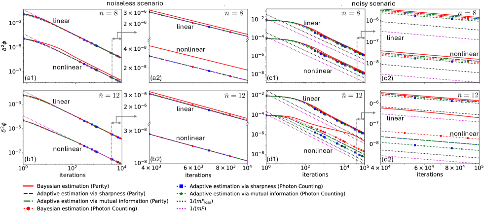
Figure 1: Performance comparison between the adaptive schemes realized by the sharpness (dashed-blue line) and mutual information (dash-dotted-green line), and Bayesian estimations (solid-red line) in [(a1)-(a2), (b1)-(b2)] noiseless and [(c1)-(c2), (d1)-(d2)] noisy scenarios. 2000 rounds of experiments are numerically simulated and all results in the plots are the average performance of them. The performance of all simulations are given in Ref. [46]. The space dimension is $11$ ($N=10$) and the true value of $\phi$ is taken as 0.2. In the noisy case the transmission rates $T_{1}=T_{2}=0.9$.

In the nonlinear case with $\bar{n}\geq N$, Eqs. (3) and (4) are only legitimate in physics when $\bar{n}$ is an integer and $N$ is the multiple of $3$. In general, the legitimate optimal states are given in the theorem below.

Theorem 3. Consider the $(N\!+\!1)$-dimensional Fock space and a fixed photon number $\bar{n}$ satisfying $\bar{n}\geq N$. The physically legitimate optimal state that provides the highest precision limit for nonlinear phase shifts reads

$$\sqrt{\frac{\bar{n}-\lfloor\bar{n}\rfloor}{2}}\!\!\left(\ket{\lfloor\bar{n}\rfloor\!+\!1\!-\!N,N}\!+\!e^{i\theta_{1}}\ket{N,\lfloor\bar{n}\rfloor\!+\!1\!-\!N}\right)$$

$$\!+\!\sqrt{\frac{1\!-\!(\bar{n}\!-\!\lfloor\bar{n}\rfloor)}{2}}\!\!\left(e^{i\theta_{2}}\ket{\lfloor\bar{n}\rfloor\!\!-\!\!N,N}\!+\!e^{i\theta_{3}}\ket{N,\lfloor\bar{n}\rfloor\!\!-\!\!N}\right)$$ (5)

when $\bar{n}\in\left[N,\left\lfloor\frac{4N}{3}\right\rfloor\!+\!\delta_{N\bmod 3,2}\right]$, and

$$\sqrt{\frac{2N\!-\!\bar{n}}{2\!\left(N\!-\!\zeta\right)}}\!\left(e^{i\theta_{1}}\!\ket{\zeta N}\!+\!e^{i\theta_{2}}\!\ket{N\zeta}\right)\!+\!\sqrt{\frac{\bar{n}\!-\!N\!-\!\zeta}{N\!-\!\zeta}}\!\ket{NN}$$ (6)

when $\bar{n}\in\left[\left\lfloor\frac{4N}{3}\right\rfloor\!+\!\delta_{N\bmod 3,2},2N\right)$. Here $\zeta:=\left\lfloor\frac{4N}{3}\right\rfloor\!-\!N\!+\!\delta_{N\bmod 3,2}$. $\lfloor\cdot\rfloor$ is the floor function, $\delta_{ij}$ is the Kronecker delta function, and $N\bmod 3$ represents the remainder of $N$ divided by $3$.

The proof of this theorem is given in Ref. [46]. In a standard Mach-Zehnder interferometer, a 50:50 beam splitter [usually characterized by $\exp(-i\pi J_{x}/2)$] exists in front of the phase shifts, and the aforementioned optimal states need to be rotated by $\exp(i\pi J_{x}/2)$ to cancel the influence of the first beam splitter. The expressions of the optimal states in the Fock space after this rotation can be found in Ref. [46].

These optimal states reveal an intriguing fact that in the finite-dimensional Fock space, the space dimension could be a metrological resource, similar to the time, particle number, and quantum correlations like entanglement. The NOON state with an unfixed average photon number $\left[(\ket{N0}+e^{i\theta}\ket{0N})/\sqrt{2}\,\right]$ cannot reveal this fact since the average photon number simultaneously increases with the increase of $N$, and thus the contribution of space dimension and photon number cannot be distinguished. The average photon numbers of the optimal states given in the theorems are fixed and the metrological gain obtained via the increase of $N$ can thus be fully attributed to the growth of the space dimension. In the meantime, the quantification of entanglement requires dimension independence due to a general belief that the same state with different dimensions should have the same amount of entanglement [47, 48], which means the obtained metrological gain can also not be attributed to the entanglement, at least in the current definition.

A more inspiring fact is that when the space dimension is large enough the given optimal states can provide better performance than the continuous-variable states with the same photon number, such as the entangled coherent state, which can never be realized by the NOON state with an unfixed average photon number [49, 50, 51]. More details of the comparison are given in Ref. [46].

A complete estimation scheme not only needs the optimal state, but also the optimal measurement to realize the predicted precision limit. Hence, the optimal measurement is always critical in quantum parameter estimation. In quantum optics, the parameterized state usually goes through a beam splitter first before the measurement is performed, such as in the Mach-Zehnder interferometer. Hence, here we follow this convention and use the one characterized by $\exp(i\pi J_{x}/2)$.

As a matter of fact, both parity and photon-counting measurements can be the optimal measurements at the asymptotic limit, yet the optimality is only valid for some specific true values of $\phi$. For the linear phase shifts the parity and photon-counting measurements are only optimal when the true value of $\phi$ is $(\theta_{1}-\theta_{2}+2k\pi)/N-\pi/2$ with $k$ any integer, and for the nonlinear phase shifts they are optimal when the true value is $\left(\theta_{1}-\theta_{2}+2k\pi\right)/N^{2}-\pi/(2N)$ in the case that $\bar{n}\leq N$. The only case presenting the true-value independence of the optimality is that $\bar{n}$ is an integer in the regime $[N,4N/3]$. Detailed calculations for both parity and photon-counting measurements are given in Ref. [46].

In practice, the true value of $\phi$ is not tunable in most cases, which strongly limits the performance of parity and photon-counting measurements as the optimal measurements. To make sure these two measurements are always optimal for any true value, the adaptive measurement has to be involved [55, 56, 57, 54, 58, 59, 60, 61, 62, 53, 63, 52, 64]. In the adaptive scheme, a tunable phase is introduced in one arm, such as mode $a$. In the linear case, the operator for it is $\exp(i\phi_{\mathrm{u}}a^{\dagger}a)$, and the operator for the total phase difference becomes $\exp(i(\phi+\phi_{\mathrm{u}})J_{z})$. In the nonlinear case, the tunable phase can be introduced via the operator $\exp(i\phi_{\mathrm{u}}(a^{\dagger}a)^{2})$ and the total phase difference then becomes $\exp(i(\phi+\phi_{\mathrm{u}})nJ_{z})$. In this paper, both average sharpness function [55, 56, 57, 54, 58, 59, 60, 61] and average mutual information [59, 60, 61, 62, 65] are used as the objective functions for the update of $\phi_{\mathrm{u}}$.

The average performance of adaptive measurement for 2000 simulations of the experiment in the case of $N=10$, together with the Bayesian estimation, are illustrated in Figs. 1(a1) and 1(b1) for the optimal states in both regimes $\bar{n}<N$ ($\bar{n}=8$) and $\bar{n}>N$ ($\bar{n}=12$). It is not surprising that the performance with nonlinear phase shifts is better than that with linear phase shifts. The true value of $\phi$ is taken as 0.2, and both parity and photon-counting measurements at this point are not optimal. From the results of the last 6000 rounds of iteration shown in Figs. 1(a2) and 1(b2), it can be seen that the Bayesian estimation cannot reach the ultimate precision quantified by the QFI (dotted purple line), which is reasonable since the Bayesian estimation for both parity and photon-counting measurements can only reach the precision quantified by CFI, and in this case, the CFI differs from the QFI as these two measurements are not optimal for this specific true value. In the adaptive scheme, the sharpness and mutual information show consistent performance. More importantly, both parity and photon-counting measurements reach the precision quantified by the QFI in both linear and nonlinear cases, indicating that adaptive measurement can overcome the dependency of the measurement optimality on the true value. Hence, utilizing the adaptive scheme, the parity and photon-counting measurements are optimal to realize the ultimate precision quantified by the QFI, regardless of the true value. More details of the adaptive measurement can be found in Ref. [46].

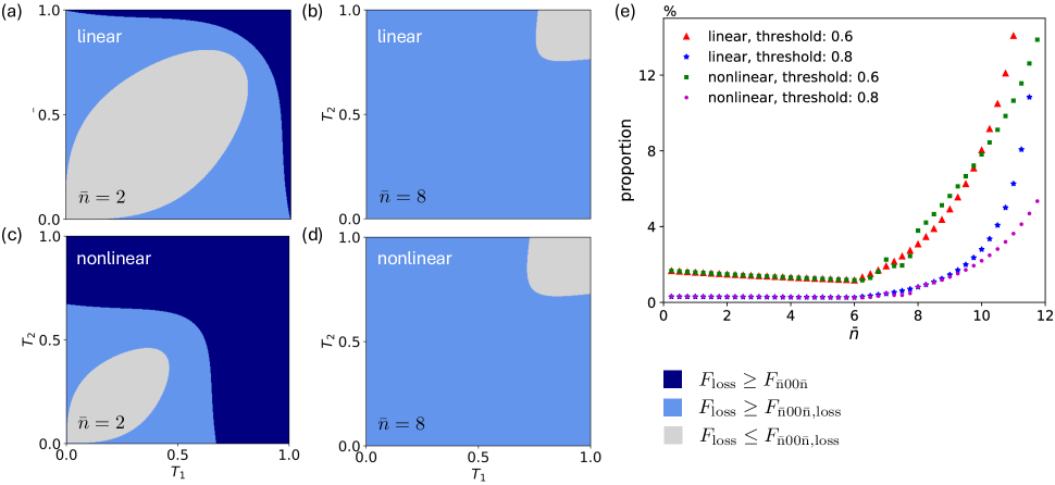
Figure 2: [(a)-(d)] Performance comparison between the optimal probe states and NOON state in (a) linear case with $\bar{n}<N$ ($\bar{n}=2$), (b) linear case with $\bar{n}>N$ ($\bar{n}=8$), (c) nonlinear case with $\bar{n}<N$ ($\bar{n}=2$), and (d) nonlinear cases with $\bar{n}>N$ ($\bar{n}=8$). (e) The variety of the proportion of the ratio $F_{\mathrm{loss}}/F$ that is larger than $0.6$ (red triangles for linear phase shifts and green squares for nonlinear phase shifts) and $0.8$ (blue stars for linear phase shifts and purple dots for nonlinear phase shifts) with the change of average input photon numbers $\bar{n}$ for both linear and nonlinear phase shifts. The Fock space dimension is $7$ ($N=6$).

The noise effect is essential to be considered in practice, and in optical phase estimation the photon loss is the major noise in general. In theory, the effect of photon loss can be modeled via a fictitious beam splitter on each arm [66, 67, 67, 68, 69, 40, 41, 70, 42, 71]. The transmission rates $T_{1}$ and $T_{2}$ of these two fictitious beam splitters represent the remains of the input photons. When $T_{1}=1$ ($T_{2}=1$), no photon leaks from the arm of mode $a$ ($b$), and all photons leak out when $T_{1}=0$ ($T_{2}=0$). The average performance of adaptive measurement under the noise of photon loss are shown in Figs. 1(c1) and 1(d1) for $\bar{n}<N$ ($\bar{n}=8$) and $\bar{n}>N$ ($\bar{n}=12$), respectively. Here $\bar{n}$ is the average photon number of the input state. When the photon loss exists, the convergence of $\delta^{2}\phi$ becomes slow, and we have to extend the iteration number in one experiment to $10^{5}$. Bayesian estimation requires more iterations to converge in the nonlinear case for parity measurement with $\bar{n}=12$, and its performance up to $10^{6}$ iterations is given in Ref. [46]. From the last $6\times 10^{4}$ iterations given in Figs. 1(c2) and 1(d2), it can be seen that both parity and photon-counting measurements cannot reach the precision quantified by the QFI, however, they can still overcome the precision given by their own CFI attained by the Bayesian estimation, and reach the maximum CFI with respect to all true values. This phenomenon immediately leads to the fact that the performance of photon-counting measurement is better than that of parity measurement under the photon loss since the maximum CFI is larger for the photon-counting measurement. The specific expressions of the maximum CFIs can be found in Ref. [46].

Compared to the NOON state with the same average photon number, i.e., $(\ket{\bar{n}0}+e^{i\theta}\ket{0\bar{n}})/\sqrt{2}$, the optimal probe states not only present a better performance in the lossless case, but also show the advantage under the photon loss for a large regime of $T_{1}$ and $T_{2}$, as illustrated in Figs. 2(a)-2(d) in the case of $N=6$. The blue regions (including both lightblue and darkblue regions) represent the regimes where the QFI of the optimal states ($F_{\mathrm{loss}}$) is larger than that of the NOON state ($F_{\mathrm{\bar{n}00\bar{n},loss}}$) under photon loss. It can be seen that the optimal states present a significant advantage for small leakage or large yet unbalanced leakage when $\bar{n}<N$. More importantly, in both linear and nonlinear cases the lossy performance of the optimal states can even overcome the lossless performance of the NOON state ($F_{\mathrm{\bar{n}00\bar{n}}}$ represents the corresponding QFI) for not very large leakage when $\bar{n}<N$ [darkblue regimes in Figs. 2(a) and 2(c)]. This advantage is remarkably significant in the nonlinear case. Hence, this result indicates that the optimal states given in this paper are better choices than the NOON state when the average photon number is limited. In the case that $\bar{n}>N$, the NOON state outperforms the optimal states when $T_{1}$ and $T_{2}$ are large, as shown in 2(b) and 2(d). However, in this case the Fock space dimension for the NOON state, which is $\bar{n}$, is larger than that of the optimal states, namely, $N$. This means more metrological resources are actually involved in the NOON state. Even though the used resources are less, the optimal states still present a better performance with the increase of the leakage. This phenomenon indicates that the given optimal states are better choices for a large photon leakage when the average photon number is large or unlimited.

The robustness of performance is another important indicator in quantum metrology. Here we use the proportion of the ratio $F_{\mathrm{loss}}/F$ ($F$ is the lossless QFI) that is higher than a given threshold with respect to all values of $T_{1}$ and $T_{2}$ as the indicator of the robustness. The variety of robustness is illustrated in the case of $N=6$ with two values of threshold ($0.6$ and $0.8$) for both linear and nonlinear phase shifts, as shown in Fig. 2(e). It can be seen that for a fixed Fock space dimension the lowest robustness occurs around the point $\bar{n}=N$, which indicates that the NOON state presents a low robustness among all the optimal states. When $\bar{n}\leq N$ the robustness does not show a significant change for both linear and nonlinear cases, however, when $\bar{n}\geq N$ it presents a remarkable improvement with the increase of $\bar{n}$, especially when $\bar{n}$ is close to $2N$. Hence, if robustness is a priority to be considered, the optimal states with a large average photon number should be chosen.

In conclusion, the optimal estimation schemes, including the optimal probe states and optimal measurements, have been provided in the finite-dimensional Fock space for both linear and nonlinear phase estimations. The given optimal probe states reveal an important phenomenon that the space dimension could be a metrological resource. Utilizing this feature, our schemes would be particularly useful in scenarios where weak light is required or the power of light is restricted, such as in the space station, due to the fact that when the photon number is fixed the measurement precision in our schemes can still be improved by only increasing the Fock space dimension. In the meantime, our schemes are not only applicable to optical systems, but also to condensed systems like cold atoms due to the extensive physical realizations of the operators of phase shifts and beam splitters. Our work provides a brand-new perspective for the improvement of phase estimation, and the given schemes could be widely applied in many mainstream quantum platforms in the near future.

Appendix A Proof of Theorem 1

In this section we provide thorough proof of Theorem 1. In the $(N+1)$-dimensional Fock space, the probe state can be expressed by

$$\ket{\psi_{\mathrm{in}}}=\sum^{N}_{i,j=0}c_{ij}\ket{ij},$$ (7)

where the coefficient $c_{ij}$ satisfies the normalization condition $\sum^{N}_{i,j=0}|c_{ij}|^{2}=1$. It is easy to see that the average photon number is

$$\bar{n}=\bra{\psi_{\mathrm{in}}}a^{\dagger}a+b^{\dagger}b\ket{\psi_{\mathrm{in}}}=\sum^{N}_{i,j=0}|c_{ij}|^{2}(i+j).$$ (8)

In the following we denote $n:=a^{\dagger}a+b^{\dagger}b$ as the the operator for total photon number.

We first consider the case of the linear phase shift. In this case, the operator for the phase shift is

$$e^{i(\phi_{a}a^{\dagger}a+\phi_{b}b^{\dagger}b)}=e^{i\frac{1}{2}\phi_{\mathrm{tot}}n}e^{i\phi J_{z}},$$ (9)

where $\phi_{\mathrm{tot}}$ is the total phase and $\phi=\phi_{a}-\phi_{b}$ is the phase difference between two arms. Here

$$J_{z}=\frac{1}{2}\left(a^{{\dagger}}a-b^{{\dagger}}b\right)$$ (10)

is a Schwinger operator. The other two Schwinger operators are

$$J_{x} = \frac{1}{2}\left(a^{{\dagger}}b+ab^{{\dagger}}\right),$$ (11)

$$J_{y} = \frac{1}{2i}\left(a^{{\dagger}}b-ab^{{\dagger}}\right).$$ (12)

Notice that $n$ commutes with all $J_{x}$, $J_{y}$, and $J_{z}$. Hence $e^{i\frac{1}{2}\phi_{\mathrm{tot}}n}$ only provides a global phase and does not affect the result. In the following the phase shift will only be expressed by $e^{i\phi J_{z}}$ for simplicity.

The QFI with respect to the phase difference for a pure parameterized state $\ket{\psi}$ can be written as

$$F=4(\bra{\partial_{\phi}\psi}\ket{\partial_{\phi}\psi}-|\bra{\partial_{\phi}\psi}\ket{\psi}|^{2}).$$ (13)

In this case, since $\ket{\psi}=e^{i\phi J_{z}}\ket{\psi_{\mathrm{in}}}$, the QFI reads

$$F= 4\left(\bra{\psi_{\mathrm{in}}}J^{2}_{z}\ket{\psi_{\mathrm{in}}}-\bra{\psi_{\mathrm{in}}}J_{z}\ket{\psi_{\mathrm{in}}}^{2}\right)$$

$$= \sum^{N}_{i,j=0}P_{ij}\left(i\!-\!j\right)^{2}\!-\!\sum^{N}_{i,j,k,l=0}P_{ij}P_{kl}\left(i\!-\!j\right)\left(k\!-\!l\right)\!,$$ (14)

where $P_{ij}:=|c_{ij}|^{2}$.

Utilizing the expression above, the problem of state optimization can be expressed by

$$\underset{P_{ij}}{\mathrm{max}} \sum^{N}_{i,j=0}P_{ij}(i-j)^{2}-\left[\sum^{N}_{i,j=0}P_{ij}(i-j)\right]^{2},$$

s.t. $$\begin{cases}P_{ij}\in[0,1],\forall i,j,\\ \sum^{N}_{i,j=0}P_{ij}=1,\\ \sum^{N}_{i,j=0}P_{ij}(i+j)=\bar{n},\end{cases}$$ (15)

where "s.t." is short for "subject to". To better solve this problem, we rewrite the subscripts of $P$ with $s=i+j$ and $d=(i-j)/2$. Here $s\in[0,2N]$ and

$$\begin{cases}d\in\left[-\frac{1}{2}s,\frac{1}{2}s\right],&s\in[0,N],\\ d\in\left[\frac{1}{2}s-N,N-\frac{1}{2}s\right],&s\in[N,2N].\end{cases}$$ (16)

In the following we denote $x_{s}:=s/2$ when $s\in[0,N]$ and $x_{s}:=N-s/2$ when $s\in[N,2N]$, which gives a uniform expression of the regime for $d$, i.e., $d\in[-x_{s},x_{s}]$. Then the optimization problem above can be rewritten into

$$\underset{P_{s,2d}}{\mathrm{max}} \leavevmode\nobreak\ 4\left[\sum^{2N}_{s=0}\sum^{x_{s}}_{d=-x_{s}}d^{2}P_{s,2d}-\left(\sum^{2N}_{s=0}\sum^{x_{s}}_{d=-x_{s}}dP_{s,2d}\right)^{2}\right],$$

s.t. $$\begin{cases}\sum^{x_{s}}_{d=-x_{s}}P_{s,2d}\in[0,1],\forall s,\\ \sum^{2N}_{s=0}\sum^{x_{s}}_{d=-x_{s}}P_{s,2d}=1,\\ \sum^{2N}_{s=0}\sum^{x_{s}}_{d=-x_{s}}sP_{s,2d}=\bar{n}.\end{cases}$$ (17)

Notice that

$$\sum^{2N}_{s=0}\sum^{x_{s}}_{d=-x_{s}}d^{2}P_{s,2d}-\left(\sum^{2N}_{s=0}\sum^{x_{s}}_{d=-x_{s}}dP_{s,2d}\right)^{2}$$

$$\leq \sum^{2N}_{s=0}\sum^{x_{s}}_{d=-x_{s}}d^{2}P_{s,2d},$$ (18)

and the equality can be attained when $\sum^{x_{s}}_{d=-x_{s}}dP_{s,2d}$ is zero. In the meantime, utilizing the condition $\sum^{x_{s}}_{d=-x_{s}}dP_{s,2d}=0$,

$$\sum^{x_{s}}_{d=-x_{s}}d^{2}P_{s,2d}=\sum^{x_{s}}_{d=-x_{s}}d^{2}P_{s,2d}-\left(\sum^{x_{s}}_{d=-x_{s}}dP_{s,2d}\right)^{2},$$ (19)

which is nothing but the variance of $d$ with respect to the probability distribution $\{P_{s,2d}\}^{x_{s}}_{d=-x_{s}}$. According to the Popoviciu’s inequality on variances [73], the maximum value of Eq. (19) can only be attained when the distribution $\{P_{s,2d}\}^{x_{s}}_{d=-x_{s}}$ is a uniform bimodal one with peaks distributed at the boundaries, namely,

$$P_{s,2d} =0,\leavevmode\nobreak\ \mathrm{for}\leavevmode\nobreak\ d\neq-x_{s},x_{s},$$ (20)

$$P_{s,-2x_{s}} =P_{s,2x_{s}}.$$ (21)

The second condition is equivalent to

$$\begin{cases}|c_{0s}|^{2}=|c_{s0}|^{2},&s\in[0,N],\\ |c_{s-N,N}|^{2}=|c_{N,s-N}|^{2},&s\in[N,2N].\end{cases}$$ (22)

Combining these two conditions, the optimization problem can be further rewritten into

$$\underset{P_{ss},P_{s,2N-s}}{\mathrm{max}}2\left[\sum^{N}_{s=0}s^{2}P_{ss}+\sum^{2N}_{s=N+1}(2N-s)^{2}P_{s,2N-s}\right]$$

$$\text{s.t.}\begin{cases}P_{ss},P_{s,2N-s}\in\left[0,\frac{1}{2}\right],\forall s\neq 0,2N,\\ P_{00},P_{2N,0}\in[0,1],\\ \sum^{N}_{s=0}P_{ss}\!+\!\sum^{2N}_{s=N+1}P_{s,2N-s}=\frac{1}{2}(1\!+\!P_{00}\!+\!P_{2N,0}),\\ \sum^{N}_{s=0}sP_{ss}\!+\!\sum^{2N}_{s=N+1}sP_{s,2N-s}=\frac{\bar{n}}{2}+NP_{2N,0}.\end{cases}$$ (23)

An equivalent writing way of the problem above is

$$\underset{P_{ss},P_{s,2N-s}}{\mathrm{min}}-2\left[\sum^{N}_{s=0}s^{2}P_{ss}+\sum^{2N}_{s=N+1}(2N-s)^{2}P_{s,2N-s}\right]$$

$$\text{s.t.}\begin{cases}P_{ss},P_{s,2N-s}\in\left[0,\frac{1}{2}\right],\forall s\neq 0,2N,\\ P_{00},P_{2N,0}\in[0,1],\\ \sum^{N}_{s=0}P_{ss}\!+\!\sum^{2N}_{s=N+1}P_{s,2N-s}=\frac{1}{2}(1\!+\!P_{00}\!+\!P_{2N,0}),\\ \sum^{N}_{s=0}sP_{ss}\!+\!\sum^{2N}_{s=N+1}sP_{s,2N-s}=\frac{\bar{n}}{2}+NP_{2N,0}.\end{cases}$$ (24)

In the following we will use the Karush-Kuhn-Tucker (KKT) conditions [74] to solve this optimization problem. For the sake of a better reading experience, we first introduce the KKT condition first. Consider the optimization problem

$$\underset{\mathbb{x}}{\mathrm{min}} f(\mathbb{x}),$$ (25)

s.t. $$g_{i}(\mathbb{x})=0,i=0,\cdots,p,$$ (27)

$$h_{i}(\mathbb{x})\leq 0,i=0,\cdots,q,$$

where $f(\mathbb{x})$ is the objective function with the real variables $\mathbb{x}$ and $h_{i}(\mathbb{x}),i=0,\cdots,p$ [$g_{i}(\mathbb{x}),i=0,\cdots,q$] is the $i$th equality (inequality) constraint. The Lagrangian function $\mathcal{L}$ for this problem is

$$\mathcal{L}=f(\mathbb{x})+\sum^{p}_{i=0}\lambda_{i}g_{i}(\mathbb{x})+\sum^{q}_{i=0}\nu_{i}h_{i}(\mathbb{x}),$$ (28)

with $\lambda_{i}\,(\nu_{i})$ the Lagrange multiplier of $i$th equality (inequality) constraint. In this case, the optimal values (denoted by $\mathbb{x}^{*}$, $\lambda_{i}^{*}$, $\nu_{i}^{*}$) must satisfy the following conditions

$$\begin{cases}\nabla f(\mathbb{x}^{*})+\sum^{p}_{i=0}\lambda^{*}_{i}\nabla g_{i}(\mathbb{x}^{*})+\sum^{q}_{i=0}\nu^{*}_{i}\nabla h_{i}(\mathbb{x}^{*})=0,\\ g_{i}(\mathbb{x}^{*})=0,\,i=0,\cdots,p,\\ h_{i}(\mathbb{x}^{*})\leq 0,\,i=0,\cdots,q,\\ \nu^{*}_{i}\geq 0,\,i=0,\cdots,q,\\ \nu^{*}_{i}h_{i}(\mathbb{x}^{*})=0,\,i=0,\cdots,q.\end{cases}$$ (29)

In the first equation $\nabla$ represents the gradient. The last two equations are the dual feasibility condition and the complementary slackness condition. These conditions are usually called the KKT conditions. More details on the KKT conditions can be found in Ref. [74].

Next, we will use the KKT conditions to find the optimal values of $P_{ss}$ and $P_{s,2N-s}$ (denoted by $P^{*}_{ss}$ and $P^{*}_{s,2N-s}$). In our problem, the Lagrangian function reads

$$\mathcal{L}= -2\sum^{N}_{s=0}s^{2}P_{ss}-2\sum^{2N}_{s=N+1}(2N-s)^{2}P_{s,2N-s}$$

$$\!-\!2\sum^{N}_{s=1}{\nu}_{s}P_{ss}\!-\!2\sum^{2N-1}_{s=N+1}{\nu}_{s}P_{s,2N-s}\!-\!\nu_{0}P_{00}\!-\!\nu_{2N}P_{2N,0}$$

$$+\lambda_{0}\left(\!P_{00}+2\sum^{N}_{s=1}\!P_{ss}+2\!\!\!\!\sum^{2N-1}_{s=N+1}P_{s,2N-s}+P_{2N,0}-1\!\!\right)$$

$$+\lambda_{1}\left(2\sum^{N}_{s=0}sP_{ss}\!+\!2\!\sum^{2N-1}_{s=N+1}sP_{s,2N-s}\!+\!2NP_{2N,0}\!-\!\bar{n}\right),$$ (30)

which indicates that the corresponding KKT conditions with respect to $P^{*}_{ss}$, $P^{*}_{s,2N-s}$, $\lambda^{*}_{0,1}$, and $\nu^{*}_{s}$ are of the form

$$\begin{cases}s^{2}-\lambda^{*}_{1}s-\lambda^{*}_{0}+\nu^{*}_{s}=0,s\in\mathbb{Z}_{[0,N]},\\ (2N\!-\!s)^{2}-\lambda^{*}_{1}s-\lambda^{*}_{0}+\nu^{*}_{s}=0,s\in\mathbb{Z}_{[N,2N]},\\ \sum^{N}_{s=0}\!P^{*}_{ss}+\sum^{2N}_{s=N+1}\!P^{*}_{s,2N-s}=\frac{1}{2}\left(1\!+\!P_{00}\!+\!P_{2N,0}\right),\\ \sum^{N}_{s=0}sP^{*}_{ss}+\sum^{2N}_{s=N+1}sP^{*}_{s,2N-s}-\frac{\bar{n}}{2}\!-\!NP_{2N,0}=0,\\ -P^{*}_{ss}\leq 0,s\in\mathbb{Z}_{[0,N]},\\ -P^{*}_{s,2N-s}\leq 0,s\in\mathbb{Z}_{[N,2N]},\\ \nu^{*}_{s}\geq 0,\forall s,\\ \nu^{*}_{s}P^{*}_{ss}=0,s\in\mathbb{Z}_{[0,N]},\\ \nu^{*}_{s}P^{*}_{s,2N-s}=s\in\mathbb{Z}_{[N,2N]}.\end{cases}$$

Here $\mathbb{Z}_{[0,N]}$ ($\mathbb{Z}_{[N,2N]}$) is the set of integers from 0 ($N$) to $N$ ($2N$). As a matter of fact, the first two conditions are equivalent when $s=N$, so does $P^{*}_{ss}$ and $P^{*}_{s,2N-s}$.

Now we apply these conditions to find the optimal values of $P^{*}_{ss}$ and $P^{*}_{s,2N-s}$. The conditions

$$\begin{cases}s^{2}-\lambda^{*}_{1}s-\lambda^{*}_{0}+\nu^{*}_{s}=0,\\ \nu^{*}_{s}\geq 0\end{cases}$$

for $s\in\mathbb{Z}_{[0,N]}$ imply that in this case

$$f_{0}(s):=s^{2}-\lambda^{*}_{1}s-\lambda^{*}_{0}\leq 0$$ (31)

Similarly, in the case that $s\in\mathbb{Z}_{[N,2N]}$, we can also obtain

$$f_{1}(s):=s^{2}-\left(4N+\lambda^{*}_{1}\right)s-\lambda^{*}_{0}+4N^{2}\leq 0$$ (32)

via the conditions

$$\begin{cases}(2N-s)^{2}-\lambda^{*}_{1}s-\lambda^{*}_{0}+\nu^{*}_{s}=0,\\ \nu^{*}_{s}\geq 0.\end{cases}$$

To simplify the discussion, in the following we take $f_{0}(s)$ and $f_{1}(s)$ as two continuous functions in the regime $s\in[0,N]$ and $s\in[N,2N]$. Notice that when $f_{0}(s)$ or $f_{1}(s)$ is less than zero, the corresponding $\nu^{*}_{s}$ has to be larger than zero since $f_{0,1}(s)+\nu^{*}_{s}=0$. In the meantime, in the KKT conditions $\nu^{*}_{s}P^{*}_{ss}=0$ ($s\in\mathbb{Z}_{[0,N]}$) and $\nu^{*}_{s}P^{*}_{s,2N-s}=0$ ($s\in\mathbb{Z}_{[N,2N]}$), and when $\nu^{*}_{s}>0$, the only possible values of $P^{*}_{ss}$ and $P^{*}_{s,2N-s}$ are zero. Hence, the nonzero $P^{*}_{ss}$ and $P^{*}_{s,2N-s}$ must correspond to a vanishing $f_{0,1}(s)$. Notice that if no zero value exists for both $f_{0}(s)$ in the regime $s\in[0,N]$ and $f_{1}(s)$ in the regime $s\in[N,2N]$, then the optimal solution $P^{*}_{ss}$ and $P^{*}_{s,2N-s}$ are always zero, which is a trivial solution and is not considered in the following discussion.

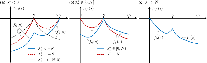
Figure 3: Behaviors of $f_{0}(s)$ and $f_{1}(s)$ for (a) $\lambda^{*}_{1}<0$, (b) $\lambda^{*}_{1}\in[0,N]$, and (c) $\lambda^{*}_{1}>N$.

Since both $f_{0}(s)$ and $f_{1}(s)$ are quadratic functions, the value of $f_{0,1}(s)$ can only be zero at the boundaries, of which the positions rely on the positions of the symmetric axes. It is easy to see that the symmetric axes for $f_{0}(s)$ and $f_{1}(s)$ are $s=\lambda^{*}_{1}/2$ and $s=2N+\lambda^{*}_{1}/2$, which means their positions are fully determined by the value of $\lambda^{*}_{1}$. Hence, the discussion below is divided into three parts according to the value of $\lambda^{*}_{1}$, i.e., $\lambda^{*}_{1}<0$, $\lambda^{*}_{1}\in\left[0,N\right]$ and $\lambda^{*}_{1}>N$, as illustrated in Fig. 3.

In case that $\lambda^{*}_{1}<0$, the axis $s=\lambda^{*}_{1}/2$ is at the left side of $y$ axis, indicating that $f_{0}(s)$ can only be zero at the right boundary $s=N$. And when it happens [dotted black and dashed red lines in Fig. 3(a)], noticing that $f_{0}(N)$ is always equivalent to $f_{1}(N)$, one can see that the symmetric axis $s=2N+\lambda^{*}_{1}/2$ cannot be at the left side of $s=3N/2$ since $f_{1}(s)$ has to be nonpositive in the regime $s\in[N,2N]$. When the symmetric axis is $s=3N/2$, i.e., $\lambda^{*}_{1}=-N$, $f_{1}(s)$ also reaches the value of zero at the right boundary $s=2N$. In this case, both $P^{*}_{NN}$ and $P^{*}_{2N,0}$ are nonzero, which means $c_{N0}$ and $c_{NN}$ is not zero. Together with the condition in Eq. (22), one can immediately obtain the form of the optimal probe state in this case

$$|c_{N0}|(e^{i\theta_{1}}\ket{0N}+e^{i\theta_{2}}\ket{N0})+|c_{NN}|\ket{NN}$$ (33)

with $\theta_{1},\theta_{2}\in[0,2\pi)$ two relative phases. Further utilizing the condition of normalization and the average photon number, $|c_{N0}|$ and $|c_{NN}|$ satisfy the equations

$$2|c_{N0}|^{2}+|c_{NN}|^{2} =1,$$ (34)

$$2N\left(|c_{N0}|^{2}+|c_{NN}|^{2}\right) =\bar{n}.$$ (35)

The corresponding solutions are

$$|c_{N0}|=\sqrt{\frac{2N-\bar{n}}{2N}},\leavevmode\nobreak\ \leavevmode\nobreak\ |c_{NN}|=\sqrt{\frac{\bar{n}-N}{N}}.$$ (36)

These solutions indicate that they are only physical when $\bar{n}\geq N$. Hence, when $\bar{n}\geq N$, one optimal probe state is of the form

$$\sqrt{\frac{2N-\bar{n}}{2N}}\left(e^{i\theta_{1}}\ket{0N}+e^{i\theta_{2}}\ket{N0}\right)+\sqrt{\frac{\bar{n}-N}{N}}\ket{NN}.$$ (37)

When the axis $s=2N+\lambda^{*}_{1}/2$ is at the right side of $s=3N/2$, $f_{1}(s)$ cannot be zero at the right boundary, indicating that the only nonzero $P^{*}_{ss}$ is just $P^{*}_{NN}$, i.e., $c_{N0}$. Therefore, the optimal probe state in this case is of the form

$$|c_{N0}|\left(\ket{0N}+e^{i\theta}\ket{N0}\right)$$ (38)

with $\theta\in[0,2\pi)$ a relative phase. Utilizing the normalization condition, it can be expressed by

$$\frac{1}{\sqrt{2}}\left(\ket{0N}+e^{i\theta}\ket{N0}\right).$$ (39)

One should notice that in this case the average photon number is $N$. Hence, this solution is only legitimate when $\bar{n}=N$. As a matter of fact, the solution in Eq. (37) reduces to Eq. (39) when $\bar{n}=N$. Therefore, these two solutions can be unified in Eq. (37).

If $f_{0}(N)$ is not zero [solid blue line in Fig. 3(a)], the only possible zero value for $f_{1}(s)$ is $f_{1}(2N)$. Hence, only $P^{*}_{2N,0}$ can be nonzero in this case, which means $c_{NN}$ is nonzero. However, one can see that the corresponding form of probe state is $c_{NN}\ket{NN}$, and the information of $\phi$ cannot be encoded into it due to the fact that $e^{i\phi J_{z}}\ket{NN}=\ket{NN}$. Hence, the optimal solution given in this case is unphysical.

In the case that $\lambda^{*}_{1}\in[0,N]$, the symmetric axis $s=2N+\lambda^{*}_{1}/2\geq 2N$, indicating that the only possible zero value for $f_{1}(s)$ is its left boundary $s=N$, as illustrated in Fig. 3(b). In this case, the left boundary of $f_{0}(s)$ can either be zero [dashed red line in Fig. 3(b)] or not [solid blue line in Fig. 3(b)], corresponding to $\lambda^{*}_{1}=N$ and $\lambda^{*}_{1}\in[0,N)$, respectively. Hence, when $\lambda^{*}_{1}=N$, $P^{*}_{00}$ and $P^{*}_{NN}$ are nonzero, i.e., $c_{00}$ and $c_{N0}$ are nonzero. Together with the condition in Eq. (22), the corresponding optimal probe state reads

$$|c_{00}|\ket{00}+|c_{N0}|(e^{i\theta_{1}}\ket{0N}+e^{i\theta_{2}}\ket{N0}).$$ (40)

Utilizing the normalization and average photon number conditions, the state above can be expressed by

$$\sqrt{\frac{N-\bar{n}}{N}}\ket{00}+\sqrt{\frac{\bar{n}}{2N}}\left(e^{i\theta_{1}}\ket{0N}+e^{i\theta_{2}}\ket{N0}\right),$$ (41)

which is only legitimate when $\bar{n}\leq N$. In the case that $\lambda^{*}_{1}\in[0,N)$, the only zero point for both $f_{0}(s)$ and $f_{1}(s)$ is at $s=N$, indicating that only $P^{*}_{NN}$ can be nonzero. In this case the optimal state is also in the form of Eq. (39), and can also be covered by Eq. (41) by taking $\bar{n}=N$.

In the case that $\lambda^{*}_{1}>N$, the symmetric axis $s=\lambda^{*}/2$ is at the right side of $s=N/2$, as illustrated in Fig. 3(c), indicating that only the left boundary is possible to be zero for $f_{0}(s)$. In the meantime, the symmetric axis for $f_{1}(s)$ is still larger than $2N$, and hence $f_{1}(s)$ cannot be zero in the regime $s\in[N,2N]$. Thus, in this case only $P^{*}_{00}$ can be zero, which corresponds to the state $c_{00}\ket{00}$. It is easy to see that as in $\ket{NN}$, the phase difference $\phi$ cannot be encoded in the state $\ket{00}$, and this solution is unphysical.

With the aforementioned discussions, the optimal probe states are solved without fully solving the KKT conditions. In summary, when $\bar{n}\in(0,N]$, the optimal probe state reads

$$\sqrt{\frac{N-\bar{n}}{N}}\ket{00}+\sqrt{\frac{\bar{n}}{2N}}\left(e^{i\theta_{1}}\ket{0N}+e^{i\theta_{2}}\ket{N0}\right)$$ (42)

and when $\bar{n}\in[N,2N)$, the optimal probe state is

$$\sqrt{\frac{2N-\bar{n}}{2N}}\left(e^{i\theta_{1}}\ket{0N}+e^{i\theta_{2}}\ket{N0}\right)+\sqrt{\frac{\bar{n}-N}{N}}\ket{NN}.$$ (43)

The theorem is then proved. $\blacksquare$

Utilizing Eq. (14), the QFI for the state (42) is in the form

$$F=\bar{n}N,$$ (44)

and for the state (43) it is

$$F=N(2N-\bar{n}).$$ (45)

Appendix B Proof of Theorem 2

B.1 General results

In this section we provide the thorough proof of Theorem 2. For two nonlinear phase shifts, the operator for the phase shift reads

$$e^{i[\phi_{a}(a^{\dagger}a)^{2}+\phi_{b}(b^{\dagger}b)^{2}]}$$

$$= e^{i\frac{1}{2}\phi_{\mathrm{tot}}[(a^{\dagger}a)^{2}+(b^{\dagger}b)^{2}]}e^{i\frac{1}{2}\phi[(a^{\dagger}a)^{2}-(b^{\dagger}b)^{2}]}$$

$$= e^{i\frac{1}{2}\phi_{\mathrm{tot}}[(a^{\dagger}a)^{2}+(b^{\dagger}b)^{2}]}e^{i\phi nJ_{z}},$$ (46)

where $\phi_{\mathrm{tot}}=\phi_{a}+\phi_{b}$ and $\phi=\phi_{a}-\phi_{b}$. Hence, the parameterized state is

$$\ket{\psi}=e^{i\frac{1}{2}\phi_{\mathrm{tot}}[(a^{\dagger}a)^{2}+(b^{\dagger}b)^{2}]}e^{i\phi nJ_{z}}\ket{\psi_{\mathrm{in}}}.$$ (47)

The corresponding QFI then reads

$$F= 4\left(\bra{\psi_{\mathrm{in}}}n^{2}J^{2}_{z}\ket{\psi_{\mathrm{in}}}-|\bra{\psi_{\mathrm{in}}}nJ_{z}\ket{\psi_{\mathrm{in}}}|^{2}\right)$$

$$= \sum^{N}_{i,j=0}P_{ij}(i^{2}\!-\!j^{2})^{2}\!-\!\sum^{N}_{i,j,k,l=0}\!\!P_{ij}P_{kl}(i^{2}\!-\!j^{2})(k^{2}\!-\!l^{2}),$$ (48)

where $P_{ij}:=|c_{ij}|^{2}$.

As in the linear case, here we rewrite $P_{ij}$ to $P_{s,2d}$ with $s=i+j$ and $d=(i-j)/2$, and the optimization problem can then be expressed by

$$\underset{P_{s,2d}}{\mathrm{max}} \leavevmode\nobreak\ 4\left[\sum^{2N}_{s=0}\sum^{x_{s}}_{d=-x_{s}}s^{2}d^{2}P_{s,2d}-\left(\sum^{2N}_{s=0}s\sum^{x_{s}}_{d=-x_{s}}dP_{s,2d}\right)^{2}\right],$$

s.t. $$\begin{cases}\sum^{x_{s}}_{d=-x_{s}}P_{s,2d}\in[0,1],\forall s,\\ \sum^{2N}_{s=0}\sum^{x_{s}}_{d=-x_{s}}P_{s,2d}=1,\\ \sum^{2N}_{s=0}\sum^{x_{s}}_{d=-x_{s}}sP_{s,2d}=\bar{n},\end{cases}$$ (49)

where $x_{s}$ is defined the same as that in the previous section, i.e., $x_{s}:=s/2$ for $s\in\mathbb{Z}_{[0,N]}$ and $x_{s}:=N-s/2$ for $s\in\mathbb{Z}_{[N,2N]}$. Notice that

$$\sum^{2N}_{s=0}\sum^{x_{s}}_{d=-x_{s}}s^{2}d^{2}P_{s,2d}-\left(\sum^{2N}_{s=0}s\sum^{x_{s}}_{d=-x_{s}}dP_{s,2d}\right)^{2}$$

$$\leq \sum^{2N}_{s=0}\sum^{x_{s}}_{d=-x_{s}}s^{2}d^{2}P_{s,2d},$$ (50)

and the equality is attained when $\sum^{x_{s}}_{d=-x_{s}}dP_{s,2d}=0$. With the condition $\sum^{x_{s}}_{d=-x_{s}}dP_{s,2d}=0$, one can further have

$$\sum^{x_{s}}_{d=-x_{s}}d^{2}P_{s,2d}=\sum^{x_{s}}_{d=-x_{s}}d^{2}P_{s,2d}-\left(\sum^{x_{s}}_{d=-x_{s}}dP_{s,2d}\right)^{2}$$ (51)

which is just the variance of $d$ with respect to the probability distribution $\{P_{s,2d}\}^{x_{s}}_{d=-x_{s}}$, similarly to the linear case. Hence, according to the Popoviciu’s inequality on variances [73], the maximum value of Eq. (51) can only be attained when

$$P_{s,2d} =0,\leavevmode\nobreak\ \mathrm{for}\leavevmode\nobreak\ d\neq-x_{s},x_{s},$$ (52)

$$P_{s,-2x_{s}} =P_{s,2x_{s}}.$$ (53)

Same as in the linear case, the second condition is equivalent to

$$\begin{cases}|c_{0s}|^{2}=|c_{s0}|^{2},&s\in\mathbb{Z}_{[0,N]},\\ |c_{s-N,N}|^{2}=|c_{N,s-N}|^{2},&s\in\mathbb{Z}_{[N,2N]}.\end{cases}$$ (54)

Combining these two conditions, the optimization problem can be further rewritten into

$$\underset{P_{ss},P_{s,2N-s}}{\mathrm{max}}2\left[\sum^{N}_{s=0}s^{4}P_{ss}+\sum^{2N}_{s=N+1}s^{2}(2N-s)^{2}P_{s,2N-s}\right]$$

$$\text{s.t.}\begin{cases}P_{ss},P_{s,2N-s}\in\left[0,\frac{1}{2}\right],\forall s\neq 0,2N,\\ P_{00},P_{2N,0}\in[0,1],\\ \sum^{N}_{s=0}P_{ss}\!+\!\sum^{2N}_{s=N+1}P_{s,2N-s}=\frac{1}{2}\left(1\!+\!P_{00}\!+\!P_{2N,0}\right)\!,\\ \sum^{N}_{s=0}sP_{ss}\!+\!\sum^{2N}_{s=N+1}sP_{s,2N-s}=\frac{\bar{n}}{2}+NP_{2N,0},\end{cases}$$

where the maximization problem is equivalent to the minimization problem as follows:

$$\underset{P_{ss},P_{s,2N-s}}{\mathrm{min}}\leavevmode\nobreak\ -2\left[\sum^{N}_{s=0}s^{4}P_{ss}+\sum^{2N}_{s=N+1}s^{2}(2N-s)^{2}P_{s,2N-s}\right]\!.$$

The Lagrangian function for the expression above reads

$$\mathcal{L}= -2\sum^{N}_{s=0}s^{4}P_{ss}-2\sum^{2N}_{s=N+1}s^{2}(2N-s)^{2}P_{s,2N-s}$$

$$-\!2\!\sum^{N}_{s=1}{\nu}_{s}P_{ss}\!-\!2\!\!\sum^{2N-1}_{s=N+1}{\nu}_{s}P_{s,2N-s}\!-\!\nu_{0}P_{00}\!-\!\nu_{2N}P_{2N,0}$$

$$\!+\!\lambda_{0}\!\left(\!\!P_{00}+2\sum^{N}_{s=1}P_{ss}+2\!\!\!\sum^{2N-1}_{s=N+1}\!\!\!\!P_{s,2N-s}+P_{2N,0}-1\!\!\right)$$

$$\!+\!\lambda_{1}\!\left(2\sum^{N}_{s=0}sP_{ss}+2\!\sum^{2N-1}_{s=N+1}sP_{s,2N-s}\!+\!2NP_{2N,0}\!-\!\bar{n}\right)\!,$$ (55)

and the corresponding KKT conditions are

$$\begin{cases}s^{4}-\lambda^{*}_{1}s-\lambda^{*}_{0}+\nu^{*}_{s}=0,s\in\mathbb{Z}_{[0,N]},\\ s^{2}(2N-s)^{2}-\lambda^{*}_{1}s-\lambda^{*}_{0}+\nu^{*}_{s}=0,s\in\mathbb{Z}_{[N,2N]},\\ \sum^{N}_{s=0}P^{*}_{ss}+\!\sum^{2N}_{s=N+1}\!P^{*}_{s,2N-s}=\!\frac{1}{2}\left(1\!+\!P_{00}\!+\!P_{2N,0}\right),\\ \sum^{N}_{s=0}sP^{*}_{ss}+\sum^{2N}_{s=N+1}sP^{*}_{s,2N-s}-\frac{\bar{n}}{2}\!-\!NP_{2N,0}=0,\\ -P^{*}_{ss}\leq 0,s\in\mathbb{Z}_{[0,N]},\\ -P^{*}_{s,2N-s}\leq 0,s\in\mathbb{Z}_{[N,2N]},\\ \nu^{*}_{s}\geq 0,\forall s,\\ \nu^{*}_{s}P^{*}_{ss}=0,s\in\mathbb{Z}_{[0,N]},\\ \nu^{*}_{s}P^{*}_{s,2N-s}=0,s\in\mathbb{Z}_{[N,2N]}.\end{cases}$$ (56)

Now define two continuous functions

$$g_{0}(s):=s^{4}-\lambda^{*}_{1}s-\lambda^{*}_{0}$$ (57)

for $s\in[0,N]$ and

$$g_{1}(s):=s^{2}(2N-s)^{2}-\lambda^{*}_{1}s-\lambda^{*}_{0}$$ (58)

for $s\in[N,2N]$. $g_{0}(s)=g_{1}(s)$ when $s=N$. As in the linear case, $P^{*}_{ss}$ is only possible to be nonzero when $g_{0}(s)=0$ due to the fact that $g_{0}(s)+\nu^{*}_{s}=0$, $\nu^{*}_{s}\geq 0$, and $\nu^{*}_{s}P^{*}_{ss}=0$ for $s\in\mathbb{Z}_{[0,N]}$. Same relation exists between $P^{*}_{s,2N-s}$ and $g_{1}(s)$ for $s\in\mathbb{Z}_{[N,2N]}$.

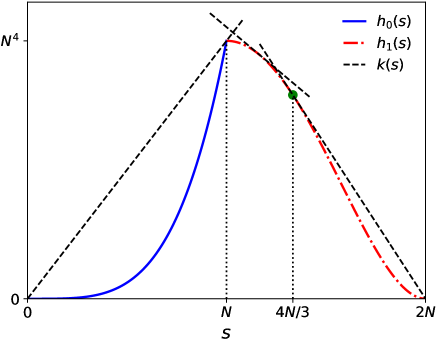
Figure 4: Schematic of locating the zero points for $g_{0}(s)$ and $g_{1}(s)$. The solid blue line, dash-dotted red line, and dashed black represent the functions $h_{0}(s)$, $h_{1}(s)$ and, $k(s)$, respectively.

Different from the linear case, here both $g_{0}(s)$ and $g_{1}(s)$ are proportional to $s^{4}$, indicating that it is not easy to solve their zero points analytically. To find the zero points, we further denote continuous functions $h_{0}(s):=s^{4}$ for $s\in[0,N]$, $h_{1}(s):=s^{2}(2N-s)^{2}$ for $s\in[N,2N]$, and $k(s):=\lambda^{*}_{1}s+\lambda^{*}_{0}$ for all values $s$, i.e., $s\in[0,2N]$. Utilizing these functions, the zero points of $g_{0}(s)$ and $g_{1}(s)$ can be found from the geometric perspective given in Fig. 4. The zero points of $g_{0}(s)$ [$g_{1}(s)$] is nothing but the intersection between $h_{0}(s)$ [$h_{1}(s)$] and $k(s)$. Due to the fact that both $h_{0}(s)$ and $h_{1}(s)$ are no larger than $k(s)$, i.e., the line of $k(s)$ (dashed black line) has to be always on top of the lines of $h_{0}(s)$ (solid blue line) and $h_{1}(s)$ (dash-dotted red line), the only possible intersections between $k(s)$ and $h_{0}(s)$ are the original point and the point of $h_{0}(N)$, as shown in the figure. Therefore, the corresponding nonzero $P^{*}_{ss}$ in this case are $P^{*}_{00}$ and $P^{*}_{NN}$, i.e., $|c_{00}|$ and $|c_{N0}|$, which means the optimal probe state can be expressed by

$$|c_{00}|\ket{00}+|c_{N0}|(e^{i\theta_{1}}\ket{0N}+e^{i\theta_{2}}\ket{N0})$$ (59)

with $\theta_{1},\theta_{2}\in[0,2\pi)$ two relative phases. Utilizing the normalization and average photon number conditions, $|c_{00}|$ and $|c_{N0}|$ are fully determined, the specific form of the optimal probe state reads

$$\sqrt{\frac{N-\bar{n}}{N}}\ket{00}+\sqrt{\frac{\bar{n}}{2N}}\left(e^{i\theta_{1}}\ket{0N}+e^{i\theta_{2}}\ket{N0}\right),$$ (60)

where $\bar{n}\leq N$. Notice that it is possible that only one intersection, either $h_{0}(0)$ or $h_{0}(N)$, exists in this case. However, the state corresponding to the nonzero $P^{*}_{00}$ is $\ket{00}$, which cannot encode the phases. In the meantime, the state corresponding to the nonzero $P^{*}_{NN}$ is contained by the expression above by taking $\bar{n}=N$.

As to $h_{1}(s)$ and $k(s)$, the situation is similar. As a matter of fact, $h_{1}(s)$ is first concave and then convex from $N$ to $2N$. On the concave part, the legitimate intersection between $h_{1}(s)$ and $k(s)$ only exists when $k(s)$ is the tangent line of $h_{1}(s)$ due to the fact that $h_{1}(s)\leq k(s)$. However, this legality stops when the intersection between the tangent line and $s$ axis reaches $2N$, as shown in Fig. 4. When it happens, the value of $s$ for the intersection between $h_{1}(s)$ and $k(s)$ (green dot in the figure) is $4N/3$. In the meantime, similarly to $h_{0}(s)$, in the regime $s\in[4N/3,2N]$, the intersections between $h_{1}(s)$ and $k(s)$ can only the point of $h_{1}(4N/3)$ and $h_{1}(2N)$. Hence, the nonzero $P^{*}_{s,2N-s}$ could be those $P^{*}_{s,2N-s}$ for $s\in[N,4N/3]$, and $P^{*}_{4N/3,2N/3}$ and $P^{*}_{2N,0}$ for $s\in[4N/3,2N]$. In the case that $s\in[N,4N/3]$, $P^{*}_{s,2N-s}$ corresponds to the coefficient $|c_{N,s-N}|$, which means the form of optimal probe state in this case reads

$$|c_{N,s-N}|\left(\ket{s-N,N}+e^{i\theta}\ket{N,s-N}\right).$$ (61)

Here $\theta\in[0,2\pi)$ is a relative phase. In the case that $s\in[4N/3,2N]$, $P^{*}_{4N/3,2N/3}$ and $P^{*}_{2N,0}$ correspond to $|c_{N,s-N}|$ and $|c_{NN}|$, and the optimal probe state can be expressed by

$$\left|c_{N,\frac{1}{3}N}\!\right|\left(\!e^{i\theta_{1}}\ket{\frac{1}{3}N,N}+e^{i\theta_{2}}\ket{N,\frac{1}{3}N}\!\right)\!+\!|c_{NN}|\ket{NN}$$ (62)

with $\theta_{1},\theta_{2}$ two relative phases. Utilizing the normalization and average photon number conditions, these two states can be specifically written as

$$\frac{1}{\sqrt{2}}\left(\ket{\bar{n}-N,N}+e^{i\theta}\ket{N,\bar{n}-N}\right)$$ (63)

for $\bar{n}\in[N,4N/3]$ and

$$\sqrt{\frac{3(2N-\bar{n})}{4N}}\left(e^{i\theta_{1}}\ket{\frac{1}{3}N,N}+e^{i\theta_{2}}\ket{N,\frac{1}{3}N}\right)$$

$$+\sqrt{\frac{3\bar{n}-4N}{2N}}\ket{NN}$$ (64)

for $\bar{n}\in[4N/3,2N]$. Similarly to the discussion of $h_{0}(s)$, it is possible that only one point between $P^{*}_{4N/3,2N/3}$ and $P^{*}_{2N,0}$ is nonzero for $s\in[4N/3,2N]$, however, $P^{*}_{2N,0}$ corresponds to $\ket{NN}$, which cannot encode the phases, and the state corresponding to $P^{*}_{4N/3,2N/3}$ is already contained in the expression above.

In summary, the optimal probe state for nonlinear phase shifts reads

$$\begin{cases}\sqrt{\frac{N-\bar{n}}{N}}\ket{00}+\sqrt{\frac{\bar{n}}{2N}}\left(e^{i\theta_{1}}\ket{0N}+e^{i\theta_{2}}\ket{N0}\right),&\bar{n}\in(0,N],\\ \frac{1}{\sqrt{2}}\left(\ket{\bar{n}-N,N}+e^{i\theta}\ket{N,\bar{n}-N}\right),&\bar{n}\in\left[N,\frac{4N}{3}\right],\\ \sqrt{\frac{3(2N-\bar{n})}{4N}}\left(e^{i\theta_{1}}\ket{\frac{1}{3}N,N}+e^{i\theta_{2}}\ket{N,\frac{1}{3}N}\right)+\sqrt{\frac{3\bar{n}-4N}{2N}}\ket{NN},&\bar{n}\in\left[\frac{4N}{3},2N\right).\end{cases}$$ (65)

The theorem is then proved. $\blacksquare$

Utilizing Eq. (48), the QFIs for the optimal states are

$$F=\begin{cases}\bar{n}N^{3},&\bar{n}\in(0,N],\\ \bar{n}^{2}(2N-\bar{n})^{2},&\bar{n}\in[N,\frac{4N}{3}],\\ \frac{32}{27}(2N-\bar{n})N^{3},&\bar{n}\in[\frac{4N}{3},2N).\end{cases}$$ (66)

B.2 Physics discussion

The optimal states for $\bar{n}\geq N$ given in Eq. (65) are only legitimate in physics when $\bar{n}-N$ and $N/3$ are nonnegative integers. However, in most cases both of them, especially the average photon number $\bar{n}$, are actually not integers. Hence, the true and legitimate optimal states in these cases have to be further discussed. In the following we provide thorough discussions on the legitimate states when $\bar{n}$ is not an integer.

Due to the discussions in the previous subsection, the types of intersections between $h_{1}(s)$ and $k(s)$ are different in the regimes $s\in[N,4N/3]$ and $s\in[4N/3,2N]$, as shown in Fig. 4. When the condition that $s\in\mathbb{Z}$ ($\mathbb{Z}$ is the set of integers) is involved, the tangent line of $h_{1}(s)$ for a continuous $s$ may not be accessible. Since $4N/3$ may not be an integer, we rewrite these two regimes into $[N,\lfloor 4N/3\rfloor]$ and $[\lfloor 4N/3\rfloor+1,2N]$. Here $\lfloor\cdot\rfloor$ is the floor function.

We first discuss the regime $s\in[N,\lfloor 4N/3\rfloor]$. In this regime, all points could be the intersection when the integer condition is not involved. Now let us denote $s_{0}$ as the intersection between $h_{1}(s)$ and its tangent line, then when the integer condition is considered, the possible intersections are actually $(\lfloor s_{0}\rfloor,h_{1}(\lfloor s_{0}\rfloor))$ and $(\lfloor s_{0}\rfloor+1,h_{1}(\lfloor s_{0}\rfloor+1))$, as shown in Fig. 5(a). Three cases exist here: either of these two points is the intersection or both of them are. Now let us first check whether both of them can be the intersections simultaneously. If this case is a legitimate one, the intersection between the line through these two points (dashed black line) and the $s$ axis has to be on the right side of the point $(2N,0)$. As a matter of fact, this line can be expressed by

$$\left[h_{1}(\lfloor s_{0}\rfloor+1)-h_{1}(\lfloor s_{0}\rfloor)\right]s-\lfloor s_{0}\rfloor h_{1}(\lfloor s_{0}\rfloor+1)$$

$$+(\lfloor s_{0}\rfloor+1)h_{1}(\lfloor s_{0}\rfloor),$$ (67)

where $h_{1}(\lfloor s_{0}\rfloor)=\lfloor s_{0}\rfloor^{2}(2N-\lfloor s_{0}\rfloor)^{2}$ and $h_{1}(\lfloor s_{0}\rfloor+1)=(\lfloor s_{0}\rfloor+1)^{2}(2N-\lfloor s_{0}\rfloor-1)^{2}$. It is easy to see that the value of $s$ for the intersection between the line above and the $s$ axis is

$$\lfloor s_{0}\rfloor+\frac{h_{1}(\lfloor s_{0}\rfloor)}{h_{1}(\lfloor s_{0}\rfloor)-h_{1}(\lfloor s_{0}\rfloor+1)}.$$ (68)

If the value of Eq. (68) is no less than $2N$, the inequality

$$\frac{h_{1}(\lfloor s_{0}\rfloor)}{h_{1}(\lfloor s_{0}\rfloor)-h_{1}(\lfloor s_{0}\rfloor+1)}\geq 2N-\lfloor s_{0}\rfloor$$ (69)

must hold. Due to the fact that $h_{1}(s)$ is a monotonic decreasing function, $h_{1}(\lfloor s_{0}\rfloor)\geq h_{1}(\lfloor s_{0}\rfloor+1)$, which means the inequality above can be further rewritten into

$$\frac{h_{1}(\lfloor s_{0}\rfloor+1)}{h_{1}(\lfloor s_{0}\rfloor)}\geq\frac{2N-\lfloor s_{0}\rfloor-1}{2N-\lfloor s_{0}\rfloor}.$$ (70)

It can be seen that $2N-\lfloor s_{0}\rfloor-1\geq 2N/3-1$ since $\lfloor s_{0}\rfloor\leq\lfloor 4N/3\rfloor\leq 4N/3$, which means $2N-\lfloor s_{0}\rfloor-1\geq 0$ for $N\geq 2$. When $N=1$, $\lfloor s_{0}\rfloor=1$ and $2N-\lfloor s_{0}\rfloor-1=0$, the inequality above naturally holds since $h_{1}(s)$ is always nonnegative. Once it holds, the inequality above can further reduce to

$$\frac{\left(\lfloor s_{0}\rfloor+1\right)^{2}(2N-\lfloor s_{0}\rfloor-1)}{\lfloor s_{0}\rfloor^{2}(2N-\lfloor s_{0}\rfloor)}\geq 1.$$ (71)

The lefthand term can be written as

$$\left(1+\frac{1}{\lfloor s_{0}\rfloor}\right)^{2}\left(1-\frac{1}{2N-\lfloor s_{0}\rfloor}\right),$$ (72)

which is obviously a monotonic decreasing function with respect to $\lfloor s_{0}\rfloor$.

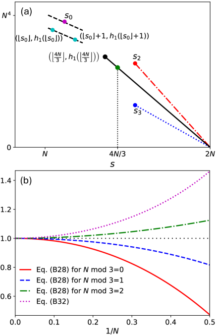
Figure 5: (a) Schematic of locating the legitimate intersections between $h_{1}(s)$ and $k(s)$. (b) Monotonicity performance of Eq. (73) for $N\bmod 3=0,1,2$, and that of Eq. (77) for $\lfloor s_{0}\rfloor=4N/3-1$.

Recall that $s_{0}\in[N,\lfloor 4N/3\rfloor]$, the minimum value of the expression above must be attained at $\lfloor 4N/3\rfloor$. However, the fact is that for different values of $N$, the expression

$$\left(1+\frac{1}{\lfloor 4N/3\rfloor}\right)^{2}\left(1-\frac{1}{2N-\lfloor 4N/3\rfloor}\right)$$ (73)

is not always no less than 1, which means the inequality (71) does not always hold. When $N\bmod 3=2$, i.e., the remainder of $N$ divided by $3$ is 2, $\lfloor 4N/3\rfloor=(4N-2)/3$ and the expression above reduces to

$$\left(1+\frac{3/N}{4-2/N}\right)^{2}\left(1-\frac{3/N}{2+2/N}\right).$$ (74)

This expression is a monotonic increasing with respect to $1/N$ [dash-dotted green line in Fig. 5(b)], and thus its minimum value is $1$, which can be attained when $1/N\rightarrow 0$. Hence, in this case the inequality (71) always holds for any value of $\lfloor s_{0}\rfloor$ satisfying $\lfloor s_{0}\rfloor\leq\lfloor 4N/3\rfloor$, indicating that both points $(\lfloor s_{0}\rfloor,h_{1}(\lfloor s_{0}\rfloor))$ and $(\lfloor s_{0}\rfloor+1,h_{1}(\lfloor s_{0}\rfloor+1))$ can be the intersections simultaneously. When $N\bmod 3=0$, the expression (73) reduces to

$$\left(1+\frac{3/N}{4}\right)^{2}\left(1-\frac{3/N}{2}\right),$$ (75)

and when $N\bmod 3=1$, it reduces to

$$\left(1+\frac{3/N}{4-1/N}\right)^{2}\left(1-\frac{3/N}{2+1/N}\right).$$ (76)

These two expressions are monotonic decreasing functions with respect to $1/N$ [solid red and dashed blue lines in Fig. 5(b)], and the minimum values are less than 1, indicating that the inequality (71) does not always hold. However, in these two cases, the inequality (71) always holds for $\lfloor s_{0}\rfloor\leq\lfloor 4N/3\rfloor-1$. This is due to the fact in this case $\lfloor s_{0}\rfloor\leq 4N/3-1$ for any value of $N$, then the lower bound of the expression (72) is

$$\left(1+\frac{3/N}{4-3/N}\right)^{2}\left(1-\frac{3/N}{2+3/N}\right).$$ (77)

This expression is a monotonic increasing function with respect to $1/N$ [dotted purple line in Fig. 5(b)]. Since its minimum value with respect to $1/N$ is $1$, this lower bound is no less than $1$, indicating that Eq. (72) is always no less than 1 for $\lfloor s_{0}\rfloor\leq\lfloor 4N/3\rfloor-1$. Hence, the inequality (71) always holds for $\lfloor s_{0}\rfloor\leq\lfloor 4N/3\rfloor-1$ regardless the value of $N$.

Based on the analysis above, one can see that the inequality (71) always holds when $\lfloor s_{0}\rfloor\leq\lfloor 4N/3\rfloor-1$, and when $\lfloor s_{0}\rfloor=\lfloor 4N/3\rfloor$, it holds for $N\bmod 3=2$ and does not hold for $N\bmod 3=0,1$. The fact that the inequality (71) always holds for $\lfloor s_{0}\rfloor\leq\lfloor 4N/3\rfloor-1$ means that in this regime $P^{*}_{\lfloor s_{0}\rfloor,2N-\lfloor s_{0}\rfloor}$ and $P^{*}_{\lfloor s_{0}\rfloor+1,2N-\lfloor s_{0}\rfloor-1}$ are nonzero, and the corresponding optimal state is of the form

$$|c_{N,\lfloor s_{0}\rfloor+1-N}|\left(\ket{\lfloor s_{0}\rfloor\!+\!1\!-\!N,N}\!+\!e^{i\theta_{1}}\ket{N,\lfloor s_{0}\rfloor\!+\!1\!-\!N}\right)$$

$$+|c_{N,\lfloor s_{0}\rfloor-N}|\left(e^{i\theta_{2}}\ket{\lfloor s_{0}\rfloor-N,N}+e^{i\theta_{3}}\ket{N,\lfloor s_{0}\rfloor-N}\right)$$

with $\theta_{1,2,3}\in[0,2\pi)$. Further utilizing the normalization condition and the average photon number condition, one can obtain that

$$|c_{N,\lfloor s_{0}\rfloor+1-N}|^{2} = \frac{\bar{n}-\lfloor s_{0}\rfloor}{2},$$ (78)

$$|c_{N,\lfloor s_{0}\rfloor-N}|^{2} = \frac{\lfloor s_{0}\rfloor+1-\bar{n}}{2}.$$ (79)

Due to the fact that both $|c_{N,\lfloor s_{0}\rfloor+1-N}|^{2}$, $|c_{N,\lfloor s_{0}\rfloor-N}|^{2}$ are nonnegative, it is easy to see that

$$\lfloor s_{0}\rfloor\leq\bar{n}\leq\lfloor s_{0}\rfloor+1,$$ (80)

which indicates that $\lfloor s_{0}\rfloor=\lfloor\bar{n}\rfloor$ due to the fact that $\bar{n}$ is not an integer. Then the optimal probe state can be written as

$$\sqrt{\frac{\bar{n}-\lfloor\bar{n}\rfloor}{2}}\left(\ket{\lfloor\bar{n}\rfloor\!+\!1\!-\!N,N}\!+\!e^{i\theta_{1}}\ket{N,\lfloor\bar{n}\rfloor\!+\!1\!-\!N}\right)$$

$$+\sqrt{\frac{1-(\bar{n}-\lfloor\bar{n}\rfloor)}{2}}\left(e^{i\theta_{2}}\ket{\lfloor\bar{n}\rfloor\!-\!N,N}\!+\!e^{i\theta_{3}}\ket{N,\lfloor\bar{n}\rfloor\!-\!N}\right),$$ (81)

where $\bar{n}$ satisfies $\lfloor\bar{n}\rfloor\leq\lfloor 4N/3\rfloor-1$. It coincides with the form in Eq. (65) for an integer $\bar{n}$.

Notice that it is possible only one point between $(\lfloor s_{0}\rfloor,h_{1}(\lfloor s_{0}\rfloor))$ and $(\lfloor s_{0}\rfloor+1,h_{1}(\lfloor s_{0}\rfloor+1))$ is the intersection. If so, only $P^{*}_{\lfloor s_{0}\rfloor,2N-\lfloor s_{0}\rfloor}$ or $P^{*}_{\lfloor s_{0}\rfloor+1,2N-\lfloor s_{0}\rfloor-1}$ is nonzero. When $P^{*}_{\lfloor s_{0}\rfloor,2N-\lfloor s_{0}\rfloor}$ is nonzero, the formula of the optimal probe state is

$$|c_{N,\lfloor s_{0}\rfloor-N}|\left(\ket{\lfloor s_{0}\rfloor-N,N}+e^{i\theta}\ket{N,\lfloor s_{0}\rfloor-N}\right).$$ (82)

The normalization and average photon number conditions give

$$|c_{N,\lfloor s_{0}\rfloor-N}|=\frac{1}{\sqrt{2}},\bar{n}=\lfloor s_{0}\rfloor.$$ (83)

This means it is only possible when $\bar{n}$ is an integer. The optimal probe state then reads

$$\frac{1}{\sqrt{2}}\left(\ket{\bar{n}-N,N}+e^{i\theta}\ket{N,\bar{n}-N}\right),$$ (84)

which is nothing but the optimal state given in Eq. (65) for $\bar{n}\in[N,4N/3]$. This result is quite reasonable since the optimal state is legitimate in physics as long as $\bar{n}$ is an integer. In the meantime it indicates that $P^{*}_{\lfloor s_{0}\rfloor,2N-\lfloor s_{0}\rfloor}$ cannot be zero when $\bar{n}$ is not an integer. In the case that $P^{*}_{\lfloor s_{0}\rfloor+1,2N-\lfloor s_{0}\rfloor-1}$ is nonzero, the same result can be obtained via a similar analysis. Hence, in the regime $\lfloor\bar{n}\rfloor\leq\lfloor 4N/3\rfloor-1$, the physical legitimate optimal probe state is the one given in Eq. (81).

In the case that $\lfloor s_{0}\rfloor=\lfloor 4N/3\rfloor$, the inequality (71) holds for $N\bmod 3=2$, which means Eq. (81) is still the optimal probe state. For $N\bmod 3=0,1$, the inequality (71) does not hold, indicating that $(\lfloor s_{0}\rfloor,h_{1}(\lfloor s_{0}\rfloor))$ and $(\lfloor s_{0}\rfloor+1,h_{1}(\lfloor s_{0}\rfloor+1))$ cannot be the intersections simultaneously. As a matter of fact, only $(\lfloor s_{0}\rfloor,h_{1}(\lfloor s_{0}\rfloor))$ can be the intersection in this case and the corresponding formula for the optimal probe state is also in the form of Eq. (84), yet an extra requirement is that $\bar{n}$ has to be an integer, which means it cannot be the intersection when $\bar{n}$ is not an integer. Combing this result with the one for $\lfloor s_{0}\rfloor\leq\lfloor 4N/3\rfloor-1$, it can be seen that the optimal probe state for $\lfloor s_{0}\rfloor\leq\lfloor 4N/3\rfloor$ is just in the form of Eq. (81), but $\bar{n}$ satisfies $\lfloor\bar{n}\rfloor\leq\lfloor 4N/3\rfloor$ for $N\bmod 3=2$ and $\bar{n}\leq\lfloor 4N/3\rfloor$ for $N\bmod 3=0,1$.

Next we discuss the regime of $s\in[\lfloor 4N/3\rfloor+1,2N)$. For $s\in[4N/3,2N)$ the intersections between $h_{1}(s)$ and $k(s)$ are $(4N/3,h_{1}(4N/3))$ and $(2N,0)$ when $s$ is continuous. In the case that $s$ is discrete, i.e., $s\in\mathbb{Z}$, $(4N/3,h_{1}(4N/3))$ may not be a legitimate point anymore. Then the position of $(\lfloor 4N/3\rfloor+1,h_{1}(\lfloor 4N/3\rfloor+1))$ becomes crucial. As shown in Fig. 5(a), if this point is above the line through the points $(\lfloor 4N/3\rfloor,h_{1}(\lfloor 4N/3\rfloor))$ and $(2N,0)$ (solid black line), demonstrated by the point $s_{2}$ in the plot, then $(\lfloor 4N/3\rfloor+1,h_{1}(\lfloor 4N/3\rfloor+1))$ and $(2N,0)$ can be the intersections simultaneously since all points on $h_{1}(s)$ are under the line through these two points (dash-dotted red line). If $(\lfloor 4N/3\rfloor+1,h_{1}(\lfloor 4N/3\rfloor+1))$ is under the solid black line, demonstrated by the point $s_{3}$ in the plot, then this point and $(2N,0)$ cannot be the intersections simultaneously since the point $(\lfloor 4N/3\rfloor,h_{1}(\lfloor 4N/3\rfloor))$ is above the line through them (dotted blue line). Hence, in this case the legitimate intersections are $(\lfloor 4N/3\rfloor,h_{1}(\lfloor 4N/3\rfloor))$ and $(2N,0)$. Based on the discussions in the case of $\lfloor s_{0}\rfloor=\lfloor 4N/3\rfloor$, we already know that $(\lfloor 4N/3\rfloor+1,h_{1}(\lfloor 4N/3\rfloor+1))$ is $s_{2}$ when $N\bmod 3=2$ and it is $s_{3}$ when $N\bmod 3=0,1$. Now we discuss them one by one.

When $N\bmod 3=2$, $(\lfloor 4N/3\rfloor+1,h_{1}(\lfloor 4N/3\rfloor+1))$ and $(2N,0)$ can be the intersections simultaneously, indicating that $P^{*}_{\lfloor 4N/3\rfloor+1,2N-\lfloor 4N/3\rfloor-1}$ and $P^{*}_{2N,0}$ are nonzero. The corresponding form of the optimal probe state then reads

$$\left|c_{N,\lfloor\frac{4N}{3}\rfloor+1-N}\right|\left(e^{i\theta_{1}}\ket{\left\lfloor\frac{4N}{3}\right\rfloor\!+\!1\!-\!N,N}\right.$$

$$+\left.e^{i\theta_{2}}\ket{N,\left\lfloor\frac{4N}{3}\right\rfloor\!+\!1\!-\!N}\right)+|c_{NN}|\ket{NN}.$$ (85)

Utilizing the normalization and average photon number conditions, it becomes

$$\sqrt{\frac{2N-\bar{n}}{2(2N-\left\lfloor\frac{4N}{3}\right\rfloor-1)}}\left(e^{i\theta_{1}}\ket{\left\lfloor\frac{4N}{3}\right\rfloor\!+\!1\!-\!N,N}\right.$$

$$+\left.e^{i\theta_{2}}\ket{N,\left\lfloor\frac{4N}{3}\right\rfloor\!+\!1\!-\!N}\right)+\sqrt{\frac{\bar{n}-\left\lfloor\frac{4N}{3}\right\rfloor-1}{2N-\left\lfloor\frac{4N}{3}\right\rfloor-1}}\ket{NN},$$ (86)

where $\bar{n}$ satisfies $\bar{n}\geq\lfloor 4N/3\rfloor+1$. In the meantime, $P^{*}_{2N,0}$ cannot be the only nonzero point due to the previous discussion. When $P^{*}_{\lfloor 4N/3\rfloor+1,2N-\lfloor 4N/3\rfloor-1}$ is the only nonzero point, the formula of the optimal state is

$$\left|c_{N,\lfloor\frac{4N}{3}\rfloor\!+\!1\!-\!N}\right|\!\left(\ket{\left\lfloor\frac{4N}{3}\right\rfloor\!\!+\!\!1\!\!-\!\!N,\!N}\!+\!e^{i\theta}\ket{N,\!\left\lfloor\frac{4N}{3}\right\rfloor\!\!+\!\!1\!\!-\!\!N}\!\right)\!\!.$$

According to the normalization and average photon number conditions, it becomes

$$\frac{1}{\sqrt{2}}\left(\ket{\left\lfloor\frac{4N}{3}\right\rfloor\!+\!1\!-\!N,N}+e^{i\theta}\ket{N,\left\lfloor\frac{4N}{3}\right\rfloor\!+\!1\!-\!N}\right),$$ (87)

where $\bar{n}=\lfloor 4N/3\rfloor+1$. It can be seen that this state is already contained in Eq. (86). And when $\bar{n}$ is not an integer, $P^{*}_{\lfloor 4N/3\rfloor+1,2N-\lfloor 4N/3\rfloor-1}$ cannot the only nonzero point.

When $N\bmod 3=0,1$, the legitimate intersections are $(\lfloor 4N/3\rfloor,h_{1}(\lfloor 4N/3\rfloor))$ and $(2N,0)$, which means that $P^{*}_{\lfloor 4N/3\rfloor,2N-\lfloor 4N/3\rfloor}$ and $P^{*}_{2N,0}$ are nonzero. The optimal state can then be written as

$$\left|c_{N,\lfloor\frac{4N}{3}\rfloor-N}\right|\left(e^{i\theta_{1}}\ket{\left\lfloor\frac{4N}{3}\right\rfloor-N,N}\right.$$

$$+\left.e^{i\theta_{2}}\ket{N,\left\lfloor\frac{4N}{3}\right\rfloor-N}\right)+|c_{NN}|\ket{NN}.$$ (88)

Utilizing the normalization and average photon number conditions, the state above can be specifically written as

$$\sqrt{\frac{2N-\bar{n}}{2(2N-\left\lfloor\frac{4N}{3}\right\rfloor)}}\left(e^{i\theta_{1}}\ket{\left\lfloor\frac{4N}{3}\right\rfloor-N,N}\right.$$

$$+\left.e^{i\theta_{2}}\ket{N,\left\lfloor\frac{4N}{3}\right\rfloor\!-\!N}\right)+\sqrt{\frac{\bar{n}-\left\lfloor\frac{4N}{3}\right\rfloor}{2N-\left\lfloor\frac{4N}{3}\right\rfloor}}\ket{NN},$$ (89)

where $\bar{n}$ satisfies $\bar{n}\geq\lfloor 4N/3\rfloor$. The state corresponding to the case that $P^{*}_{\lfloor 4N/3\rfloor,2N-\lfloor 4N/3\rfloor}$ is the only nonzero point is of the form

$$\frac{1}{\sqrt{2}}\left(\ket{\left\lfloor\frac{4N}{3}\right\rfloor-N,N}+e^{i\theta}\ket{N,\left\lfloor\frac{4N}{3}\right\rfloor-N}\right)$$ (90)

with $\bar{n}=\lfloor 4N/3\rfloor$, which is already contained in Eq. (89). And when $\bar{n}$ is not an integer, $P^{*}_{\lfloor 4N/3\rfloor,2N-\lfloor 4N/3\rfloor}$ cannot the only nonzero point.

In summary, for $N\bmod 3=2$, the optimal state is Eq. (81) for $\lfloor\bar{n}\rfloor\leq\lfloor 4N/3\rfloor$, which is equivalent to $\bar{n}<\lfloor 4N/3\rfloor+1$, and Eq. (86) for $\bar{n}\geq\lfloor 4N/3\rfloor+1$. As a matter of fact, taking $\bar{n}=\lfloor 4N/3\rfloor+1$ in Eq. (81), it just reduces to the state in Eq. (87). Hence, one can also state that the optimal state is Eq. (81) for $\bar{n}\leq\lfloor 4N/3\rfloor+1$. For $N\bmod 3=0,1$, the optimal state is Eq. (81) for $\bar{n}\leq\lfloor 4N/3\rfloor$ and Eq. (89) for $\bar{n}\geq\lfloor 4N/3\rfloor$. Utilizing the Kronecker delta function $\delta_{N\bmod 3,2}$, i.e., $\delta_{N\bmod 3,2}=1$ for $N\bmod 3=2$ and 0 for others, the optimal states can be unified into the following expressions:

$$\begin{cases}\sqrt{\frac{\bar{n}-\lfloor\bar{n}\rfloor}{2}}\left(\ket{\lfloor\bar{n}\rfloor\!+\!1\!-\!N,N}\!+\!e^{i\theta_{1}}\ket{N,\lfloor\bar{n}\rfloor\!+\!1\!-\!N}\right)&\\ +\sqrt{\frac{1-(\bar{n}-\lfloor\bar{n}\rfloor)}{2}}\left(e^{i\theta_{2}}\ket{\lfloor\bar{n}\rfloor\!-\!N,N}\!+\!e^{i\theta_{3}}\ket{N,\lfloor\bar{n}\rfloor\!-\!N}\right),&\bar{n}\in\left[N,\left\lfloor\frac{4N}{3}\right\rfloor\!+\!\delta_{N\bmod 3,2}\right],\\ \\ \sqrt{\frac{2N-\bar{n}}{2\left(2N-\left\lfloor\frac{4N}{3}\right\rfloor-\delta_{N\bmod 3,2}\right)}}\left(e^{i\theta_{1}}\ket{\left\lfloor\frac{4N}{3}\right\rfloor\!-\!N\!+\!\delta_{N\bmod 3,2},N}\right.\\ +\left.e^{i\theta_{2}}\ket{N,\left\lfloor\frac{4N}{3}\right\rfloor\!-\!N\!+\!\delta_{N\bmod 3,2}}\right)+\sqrt{\frac{\bar{n}-\left\lfloor\frac{4N}{3}\right\rfloor-\delta_{N\bmod 3,2}}{2N-\left\lfloor\frac{4N}{3}\right\rfloor-\delta_{N\bmod 3,2}}}\ket{NN},&\bar{n}\in\left[\left\lfloor\frac{4N}{3}\right\rfloor\!+\!\delta_{N\bmod 3,2},2N\right).\end{cases}$$ (91)

The theorem is then proved. $\blacksquare$

Utilizing Eq. (48), the expressions of QFI for the optimal states above are

$$F= (\bar{n}-\lfloor\bar{n}\rfloor)(\lfloor\bar{n}\rfloor+1)^{2}(2N-\lfloor\bar{n}\rfloor-1)^{2}$$

$$+(1+\lfloor\bar{n}\rfloor-\bar{n})\lfloor\bar{n}\rfloor^{2}(2N-\lfloor\bar{n}\rfloor)^{2}$$ (92)

for $\bar{n}\in\left[N,\left\lfloor\frac{4N}{3}\right\rfloor\!+\!\delta_{N\bmod 3,2}\right]$, and

$$F= \frac{2N-\bar{n}}{2N-\left\lfloor\frac{4N}{3}\right\rfloor\!-\!\delta_{N\bmod 3,2}}\left(\left\lfloor\frac{4N}{3}\right\rfloor\!+\!\delta_{N\bmod 3,2}\right)^{2}$$

$$\times\left(2N-\left\lfloor\frac{4N}{3}\right\rfloor\!-\!\delta_{N\bmod 3,2}\right)^{2}$$ (93)

for $\bar{n}\in\left[\left\lfloor\frac{4N}{3}\right\rfloor\!+\!\delta_{N\bmod 3,2},2N\right)$.

Appendix C Optimal probe states in the Mach-Zehnder interferometer

In the previous sections we provide the optimal probe states for linear and nonlinear phase shifts. In practice, the phase estimation is usually performed in the Mach-Zehnder interferometer (MZI), in which a beam splitter exists in front of the phase shifts. Here we use a 50:50 beam splitter represented by the operator $\exp(-i\frac{\pi}{2}J_{x})$. Hence, the optimal probe state must take the form $\exp(i\frac{\pi}{2}J_{x})\ket{\psi_{\mathrm{opt}}}$ with $\ket{\psi_{\mathrm{opt}}}$ the optimal states we previously gave.

C.1 Linear case

For a two-mode Fock state $\ket{n_{1}n_{2}}$, $\exp(i\frac{\pi}{2}J_{x})\ket{n_{1}n_{2}}$ can be calculated as

$$e^{i\frac{\pi}{2}J_{x}}\ket{n_{1}n_{2}}$$

$$= \left(\frac{1}{\sqrt{2}}\right)^{n_{1}+n_{2}}\sum^{n_{1}}_{k=0}\sum^{n_{2}}_{l=0}\binom{n_{1}}{k}\binom{n_{2}}{l}i^{k+l}\frac{\sqrt{(n_{1}-k+l)!}}{\sqrt{n_{1}!}}$$

$$\times\frac{\sqrt{(n_{2}+k-l)!}}{\sqrt{n_{2}!}}\ket{n_{1}-k+l,n_{2}+k-l},$$ (94)

where $\ket{n_{1}}=\frac{1}{\sqrt{n_{1}!}}(a^{{\dagger}})^{n_{1}}\ket{0}$, $\ket{n_{2}}=\frac{1}{\sqrt{n_{2}!}}(b^{{\dagger}})^{n_{2}}\ket{0}$, and

$$e^{i\frac{\pi}{2}J_{x}}a^{\dagger}e^{-i\frac{\pi}{2}J_{x}} = \frac{1}{\sqrt{2}}\left(a^{\dagger}+ib^{\dagger}\right),$$ (95)

$$e^{i\frac{\pi}{2}J_{x}}b^{\dagger}e^{-i\frac{\pi}{2}J_{x}} = \frac{1}{\sqrt{2}}\left(b^{\dagger}+ia^{\dagger}\right)$$ (96)

have been applied.

In the case of $\bar{n}\leq N$, the optimal state without the beam splitter is given in Eq. (42). Therefore, with Eq. (94) it can be seen that the optimal state in the MZI reads

$$\sqrt{1-\frac{\bar{n}}{N}}\ket{00}+2^{-\frac{1}{2}(N+1)}\sqrt{\frac{\bar{n}}{N}}\sum^{N}_{k=0}i^{k}\binom{N}{k}^{\frac{1}{2}}$$

$$\times\left(e^{i\theta_{1}}\ket{k,N-k}+e^{i\theta_{2}}\ket{N-k,k}\right).$$ (97)

In the case of $\bar{n}\geq N$, the optimal state without the beam splitter is given in Eq. (43). Hence, the optimal state in the MZI is of the form

$$2^{-\frac{1}{2}(N+1)}\!\!\!\sqrt{2-\frac{\bar{n}}{N}}\sum_{k=0}^{N}i^{k}\binom{N}{k}^{\frac{1}{2}}\left(e^{i\theta_{1}}\ket{k,N-k}\right.$$

$$\left.+e^{i\theta_{2}}\ket{N\!-\!k,k}\right)\!+\!2^{-N}\sqrt{\frac{\bar{n}}{N}-1}\sum^{N}_{k,l=0}\binom{N}{k}\binom{N}{l}i^{k+l}$$

$$\times\frac{\sqrt{(N-k+l)!(N+k-l)!}}{N!}\ket{N\!-\!k+\!l,N\!+\!k\!-\!l}.$$ (98)

C.2 Nonlinear case

Now we provide the optimal probe states in the MZI with nonlinear phase shifts. In the case that $\bar{n}\leq N$, the optimal probe state without the beam splitter is the same as that in the linear case. Hence, the optimal probe state in the MZI also takes the form of Eq. (97).

When $\bar{n}\geq N$, the legitimate optimal probe states without the beam splitter are given in Eq. (91). Utilizing Eq. (94), the optimal state in the MZI in the regime $\bar{n}\in\left[N,\left\lfloor\frac{4N}{3}\right\rfloor+\delta_{N\bmod 3,2}\right]$ can be expressed by

$$2^{-(\frac{1}{2}\lfloor\bar{n}\rfloor+1)}\sqrt{\bar{n}-\lfloor\bar{n}\rfloor}\sum^{\lfloor\bar{n}\rfloor\!+\!1\!-\!N}_{k=0}\sum^{N}_{l=0}\binom{\lfloor\bar{n}\rfloor\!+\!1\!-\!N}{k}\binom{N}{l}i^{k+l}\sqrt{\frac{(\lfloor\bar{n}\rfloor+1-N-k+l)!(N+k-l)!}{N!(\lfloor\bar{n}\rfloor+1-N)!}}$$

$$\times\left(\ket{\lfloor\bar{n}\rfloor+1-N-k+l,N+k-l}+e^{i\theta_{1}}\ket{N+k-l,\lfloor\bar{n}\rfloor+1-N-k+l}\right)$$

$$+2^{-\frac{1}{2}(\lfloor\bar{n}\rfloor+1)}\sqrt{1-(\bar{n}-\lfloor\bar{n}\rfloor)}\sum^{\lfloor\bar{n}\rfloor-N}_{s=0}\sum^{N}_{t=0}\binom{\lfloor\bar{n}\rfloor-N}{s}\binom{N}{t}i^{s+t}\sqrt{\frac{(\lfloor\bar{n}\rfloor-N-s+t)!(N+s-t)!}{(\lfloor\bar{n}\rfloor-N)!N!}}$$

$$\times\left(e^{i\theta_{2}}\ket{\lfloor\bar{n}\rfloor-N-s+t,N+s-t}+e^{i\theta_{3}}\ket{N+s-t,\lfloor\bar{n}\rfloor-N-s+t}\right).$$ (99)

In the regime $\bar{n}\in\left[\left\lfloor\frac{4N}{3}\right\rfloor+\delta_{N\bmod 3,2},2N\right)$, the optimal probe state in the MZI reads

$$2^{-N}\sqrt{\frac{\bar{n}-\zeta-N}{N-c}}\sum^{N}_{k,l=0}\binom{N}{k}\binom{N}{l}i^{k+l}\frac{\sqrt{(N-k+l)!(N+k-l)!}}{N!}\ket{N-k+l,N+k-l}$$

$$+2^{-\frac{1}{2}(N+\zeta+1)}\sqrt{\frac{2N-\bar{n}}{N-\zeta}}\sum^{\zeta}_{s=0}\sum^{N}_{t=0}\binom{\zeta}{s}\binom{N}{t}i^{s+t}\sqrt{\frac{(\zeta-s+t)!(N+s-t)!}{\zeta!N!}}$$

$$\times\left(e^{i\theta_{1}}\ket{\zeta-s+t,N+s-t}+e^{i\theta_{2}}\ket{N+s-t,\zeta-s+t}\right),$$ (100)

where $\zeta:=\left\lfloor\frac{4N}{3}\right\rfloor-N+\delta_{N\bmod 3,2}$.

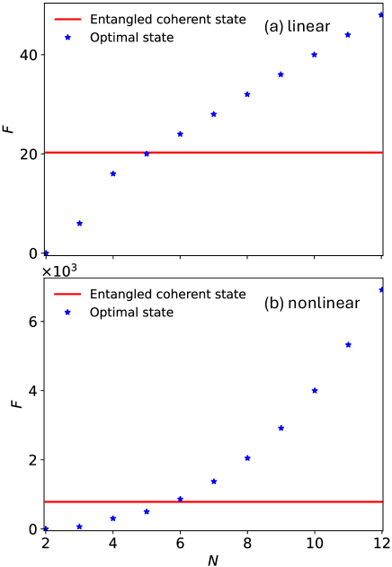
Figure 6: Comparison of the QFI between the entangled coherent state (red line) and the optimal states given in this paper (blue stars) for (a) linear phase shifts and (b) nonlinear phase shifts. The average photon number $\bar{n}=4$.

Appendix D Comparison with entangled coherent state

The entangled coherent state is a very useful state in quantum metrology, which is of the form [49, 50, 51]

$$C_{\alpha}\left(\ket{\alpha 0}+\ket{0\alpha}\right),$$ (101)

where $C_{\alpha}=1/\sqrt{2(1+e^{-|\alpha|^{2}})}$ is the normalization coefficient, and $\ket{\alpha}$ is coherent state.

For the linear phase shifts, the QFI in Eq. (14) can be expressed by

$$F_{\mathrm{lin}}=2|C_{\alpha}|^{2}|\alpha|^{2}\left(1+|\alpha|^{2}\right)$$ (102)

due to the fact that $\expectationvalue{J^{2}_{z}}=|C_{\alpha}|^{2}|\alpha|^{2}\left(1+|\alpha|^{2}\right)/2$ and $\expectationvalue{J_{z}}=0$. Here the average photon number $\bar{n}=2|C_{\alpha}|^{2}|\alpha|^{2}$. And for nonlinear phase shifts, the QFI can be calculated via Eq. (48). In this case

$$\expectationvalue{n^{2}J^{2}_{z}}=\frac{1}{2}|C_{\alpha}|^{2}|\alpha|^{2}\left(|\alpha|^{6}+6|\alpha|^{4}+7|\alpha|^{2}+1\right),$$ (103)

and $\expectationvalue{nJ_{z}}=0$, then the QFI reads

$$F_{\mathrm{non}}=2|C_{\alpha}|^{2}|\alpha|^{2}\left(|\alpha|^{6}+6|\alpha|^{4}+7|\alpha|^{2}+1\right).$$ (104)

Both $F_{\mathrm{lin}}$ and $F_{\mathrm{non}}$ can be rewritten into a function of $\bar{n}$ via the equation $\bar{n}=|\alpha|^{2}/(1+e^{-|\alpha|^{2}})$. The QFI for the entangled coherent state and the optimal states given in this paper are shown in Figs. 6(a) for linear phase shifts and 6(b) for nonlinear phase shifts in the case of $\bar{n}=4$. It can be seen that with the increase of $N$, the QFI of the optimal states given in this paper would overcome that of the entangled coherent state, which could never be realized by the NOON state $(\ket{\bar{n}0}+e^{i\theta}\ket{0\bar{n}})/\sqrt{2}$ [49, 50, 51].

Appendix E Parity measurement

E.1 Linear case

The parity operator for the $a$th mode is

$$\Pi_{a}=e^{i\pi a^{\dagger}a}=e^{i\frac{\pi}{2}n}e^{i\pi J_{z}},$$ (105)

where $n=a^{\dagger}a+b^{\dagger}b$ is the operator for the total photon number and commutes with all $J_{x}$, $J_{y}$, and $J_{z}$. Recall that the state before the measurement is $e^{i\frac{\pi}{2}J_{x}}e^{i\phi J_{z}}\ket{\psi_{\mathrm{in}}}$. Then the expected value of the parity operator reads

$$\expectationvalue{\Pi_{a}} =\bra{\psi_{\mathrm{in}}}e^{-i\phi J_{z}}e^{-i\frac{\pi}{2}J_{x}}e^{i\frac{\pi}{2}n}e^{i\pi J_{z}}e^{i\frac{\pi}{2}J_{x}}e^{i\phi J_{z}}\ket{\psi_{\mathrm{in}}}$$

$$=\bra{\psi_{\mathrm{in}}}e^{i\frac{\pi}{2}n}e^{-i\phi J_{z}}e^{-i\pi J_{y}}e^{i\phi J_{z}}\ket{\psi_{\mathrm{in}}},$$ (106)

where the equality $e^{-i\frac{\pi}{2}J_{x}}e^{i\pi J_{z}}e^{i\frac{\pi}{2}J_{x}}=e^{-i\pi J_{y}}$ has been applied.

In the case that $\bar{n}\leq N$, the optimal probe state reads

$$\sqrt{\frac{N-\bar{n}}{N}}\ket{00}+\sqrt{\frac{\bar{n}}{2N}}\left(e^{i\theta_{1}}\ket{0N}+e^{i\theta_{2}}\ket{N0}\right).$$ (107)

Substituting it into Eq. (106), and further utilizing

$$e^{i\phi J_{z}}\ket{n_{1}n_{2}}=e^{i\frac{\phi}{2}(n_{1}-n_{2})}\ket{n_{1}n_{2}},$$ (108)

where $\ket{n_{1(2)}}$ is a Fock state with respect to mode $a$ ($b$), and

$$e^{-i\pi J_{y}}\ket{n_{1}n_{2}}$$

$$=\frac{\left(e^{-i\pi J_{y}}a^{\dagger}e^{i\pi J_{y}}\right)^{n_{1}}}{\sqrt{n_{1}!}}\frac{\left(e^{-i\pi J_{y}}b^{\dagger}e^{i\pi J_{y}}\right)^{n_{2}}}{\sqrt{n_{2}!}}\ket{00}$$

$$=\frac{\left(-a^{\dagger}\right)^{n_{2}}}{\sqrt{n_{2}!}}\frac{\left(b^{\dagger}\right)^{n_{1}}}{\sqrt{n_{1}!}}\ket{00}$$

$$=e^{i\pi n_{2}}\ket{n_{2}n_{1}},$$ (109)

where $e^{-i\pi J_{y}}a^{\dagger}e^{i\pi J_{y}}=b^{\dagger}$ and $e^{-i\pi J_{y}}b^{\dagger}e^{i\pi J_{y}}=-a^{\dagger}$ have been applied, one can obtain the expression

$$\expectationvalue{\Pi_{a}}=1-\frac{\bar{n}}{N}\left(1-\cos\beta_{1}\right),$$ (110)

where

$$\beta_{1}:=\theta_{2}-\theta_{1}+\frac{\pi}{2}N+\phi N.$$ (111)

The variance $\delta^{2}\phi$ of measuring $\phi$ via $\expectationvalue{\Pi_{a}}$ can be evaluated through the error propagation relation

$$\delta^{2}\phi=\frac{\expectationvalue{\Pi^{2}_{a}}-\expectationvalue{\Pi_{a}}^{2}}{\left|\partial_{\phi}\expectationvalue{\Pi_{a}}\right|^{2}}.$$ (112)

As a matter of fact, here $\expectationvalue{\Pi^{2}_{a}}=1$ due to the fact that $\Pi^{2}_{a}=\openone$ with $\openone$ the identity operator. Applying the expression of $\expectationvalue{\Pi_{a}}$, $\delta^{2}\phi$ can be expressed by

$$\delta^{2}\phi=\frac{1}{\bar{n}N}\frac{2(1-\cos\beta_{1})}{\sin^{2}\beta_{1}}-\frac{1}{N^{2}}\frac{(1-\cos\beta_{1})^{2}}{\sin^{2}\beta_{1}}.$$ (113)

One may notice that $\delta^{2}\phi$ depends on $\phi$, indicating that the true value of $\phi$ could affect the performance of parity measurement. When the value of $\beta_{1}$ is very close to $2k\pi$ ($k$ is any integer), i.e., $\beta_{1}=2k\pi+\delta\beta_{1}$ with $\delta\beta_{1}$ a small quantity, $\delta^{2}\phi$ reduces to

$$\delta^{2}\phi=\frac{1}{\bar{n}N}-\frac{1}{4N^{2}}\delta^{2}\beta_{1},$$ (114)

which means that

$$\lim_{\delta\beta_{1}\rightarrow 0}\delta^{2}\phi=\frac{1}{\bar{n}N}.$$ (115)

Noticing that the QFI in this case is $\bar{n}N$, the parity measurement is optimal when the value of $\beta_{1}$ equals to $2k\pi$, which means the true value of $\phi$ ($\phi_{\mathrm{true}}$) has to be in the form

$$\phi_{\mathrm{true}}=\frac{1}{N}\left(\theta_{1}-\theta_{2}+2k\pi\right)-\frac{\pi}{2},\leavevmode\nobreak\ k\in\mathbb{Z},$$ (116)

where $\mathbb{Z}$ is the set of integers.

Now we discuss the performance of parity measurement from the perspective of the classical Fisher information (CFI), which is

$$I=\frac{\left(\partial_{\phi}P_{+}\right)^{2}}{P_{+}}+\frac{\left(\partial_{\phi}P_{-}\right)^{2}}{P_{-}},$$ (117)

where $P_{\pm}$ is the probability of obtaining the result $\pm 1$ by measuring $\expectationvalue{\Pi_{a}}$. It can be seen that

$$P_{+} =1-\frac{\bar{n}}{2N}\left(1-\cos\beta_{1}\right),$$ (118)

$$P_{-} =\frac{\bar{n}}{2N}\left(1-\cos\beta_{1}\right),$$ (119)

which can be obtained via the equations $\expectationvalue{\Pi_{a}}=P_{+}-P_{-}$ and $P_{+}+P_{-}=1$. With these expressions, the CFI can be calculated as

$$I=\frac{\bar{n}N^{2}\sin^{2}\beta_{1}}{(1-\cos\beta_{1})\left[2N-\bar{n}(1-\cos\beta_{1})\right]},$$ (120)

which directly gives

$$\lim_{\beta_{1}\rightarrow 2k\pi}I=\bar{n}N.$$ (121)

Therefore, this equation means that the CFI can reach the QFI when the true value of $\phi$ satisfies Eq. (116).

In the case that $\bar{n}\geq N$, the optimal probe state reads

$$\sqrt{\frac{2N-\bar{n}}{2N}}\left(e^{i\theta_{1}}\ket{0N}+e^{i\theta_{2}}\ket{N0}\right)+\sqrt{\frac{\bar{n}-N}{N}}\ket{NN}.$$

The value of $\expectationvalue{\Pi_{a}}$ can then be calculated as

$$\expectationvalue{\Pi_{a}}=\frac{\bar{n}-N}{N}+\frac{2N-\bar{n}}{N}\cos\beta_{1}.$$ (122)

Utilizing the error propagation relation, $\delta^{2}\phi$ can be expressed by

$$\delta^{2}\phi=\frac{2(1-\cos\beta_{1})}{N(2N-\bar{n})\sin^{2}\beta_{1}}-\frac{\left(1-\cos\beta_{1}\right)^{2}}{N^{2}\sin^{2}\beta_{1}},$$ (123)

and its limit is

$$\lim_{\beta_{1}\rightarrow 2k\pi}\delta^{2}\phi=\frac{1}{N(2N-\bar{n})}.$$ (124)

In this case, the QFI is just $N(2N-\bar{n})$, indicating that the parity measurement is optimal when

$$\phi_{\mathrm{true}}=\frac{1}{N}\left(\theta_{1}-\theta_{2}+2k\pi\right)-\frac{\pi}{2}.$$ (125)

From the perspective of CFI, the conditional probability $P_{\pm}$ in this case reads

$$P_{+} =1-\frac{2N-\bar{n}}{2N}\left(1-\cos\beta_{1}\right),$$ (126)

$$P_{-} =\frac{2N-\bar{n}}{2N}\left(1-\cos\beta_{1}\right).$$ (127)

The CFI is

$$I=\frac{(2N-\bar{n})N^{2}\sin^{2}\beta_{1}}{(1-\cos\beta_{1})\left[2N-(2N-\bar{n})(1-\cos\beta_{1})\right]},$$ (128)

and $\lim_{\beta_{1}\rightarrow 2k\pi}I=(2N-\bar{n})N$.

E.2 Nonlinear case

In the nonlinear case, the state before the measurement is $e^{i\frac{\pi}{2}J_{x}}e^{i\frac{1}{2}\phi_{\mathrm{tot}}[(a^{\dagger}a)^{2}+(b^{\dagger}b)^{2}]}e^{i\phi nJ_{z}}\ket{\psi_{\mathrm{in}}}$. Then the expectation of the parity operator is

$$\expectationvalue{\Pi_{a}}= \bra{\psi_{\mathrm{in}}}e^{-i\phi nJ_{z}}e^{-i\frac{1}{2}\phi_{\mathrm{tot}}[(a^{\dagger}a)^{2}+(b^{\dagger}b)^{2}]}e^{-i\frac{\pi}{2}J_{x}}$$

$$\times e^{i\frac{\pi}{2}n}e^{i\pi J_{z}}e^{i\frac{\pi}{2}J_{x}}e^{i\frac{1}{2}\phi_{\mathrm{tot}}[(a^{\dagger}a)^{2}+(b^{\dagger}b)^{2}]}e^{i\phi nJ_{z}}\ket{\psi_{\mathrm{in}}}$$

$$= \bra{\psi_{\mathrm{in}}}e^{i\frac{\pi}{2}n}e^{-i\phi nJ_{z}}e^{-i\frac{1}{2}\phi_{\mathrm{tot}}[(a^{\dagger}a)^{2}+(b^{\dagger}b)^{2}]}e^{-i\pi J_{y}}$$

$$\times e^{i\frac{1}{2}\phi_{\mathrm{tot}}[(a^{\dagger}a)^{2}+(b^{\dagger}b)^{2}]}e^{i\phi nJ_{z}}\ket{\psi_{\mathrm{in}}},$$ (129)

where the equality $e^{-i\frac{\pi}{2}J_{x}}e^{i\pi J_{z}}e^{i\frac{\pi}{2}J_{x}}=e^{-i\pi J_{y}}$ has been applied.

In the case of $\bar{n}\leq N$, the optimal probe state reads

$$\sqrt{\frac{N-\bar{n}}{N}}\ket{00}+\sqrt{\frac{\bar{n}}{2N}}\left(e^{i\theta_{1}}\ket{0N}+e^{i\theta_{2}}\ket{N0}\right).$$ (130)

Utilizing Eq. (109) and the equality $e^{i\phi nJ_{z}}\ket{n_{1}n_{2}}=e^{i\frac{1}{2}\left(n_{1}^{2}-n_{2}^{2}\right)\phi}\ket{n_{1}n_{2}}$, $\expectationvalue{\Pi_{a}}$ can be expressed by

$$\expectationvalue{\Pi_{a}}=1-\frac{\bar{n}}{N}\left(1-\cos\beta_{2}\right),$$ (131)

where

$$\beta_{2}:=\theta_{2}-\theta_{1}+\frac{\pi}{2}N+\phi N^{2}.$$ (132)

The variance $\delta^{2}\phi$ obtained from the error propagation relation can be written as

$$\delta^{2}\phi=\frac{1}{\bar{n}N^{3}}\frac{2(1-\cos\beta_{2})}{\sin^{2}\beta_{2}}-\frac{1}{N^{4}}\frac{(1-\cos\beta_{2})^{2}}{\sin^{2}\beta_{2}}.$$ (133)

Its limit for $\beta_{2}\rightarrow 2k\pi$ is

$$\lim_{\beta_{2}\rightarrow 2k\pi}\delta^{2}\phi=\frac{1}{\bar{n}N^{3}}.$$ (134)

In this case, the QFI reads $\bar{n}N^{3}$, therefore, same with the linear case, the parity measurement is optimal when the value of $\beta_{2}$ approaches to $2k\pi$, which means the true value of $\phi$ ($\phi_{\mathrm{true}}$) needs to be

$$\phi_{\mathrm{true}}=\frac{1}{N^{2}}\left(\theta_{1}-\theta_{2}+2k\pi\right)-\frac{\pi}{2N},\leavevmode\nobreak\ k\in\mathbb{Z}.$$ (135)

From the perspective of CFI, the probabilities $P_{+}$ and $P_{-}$ read

$$P_{+} =1-\frac{\bar{n}}{2N}\left(1-\cos\beta_{2}\right),$$ (136)

$$P_{-} =\frac{\bar{n}}{2N}\left(1-\cos\beta_{2}\right),$$ (137)

and the CFI can then be expressed by

$$I=\frac{\bar{n}N^{4}\sin^{2}\beta_{2}}{(1-\cos\beta_{2})\left[2N-\bar{n}(1-\cos\beta_{2})\right]}.$$ (138)

It can be further found that

$$\lim_{\beta_{2}\rightarrow 2k\pi}I=\bar{n}N^{3}.$$ (139)

In the case of $\bar{n}\geq N$, we demonstrate a simple case that $\bar{n}\in[N,4N/3]$ is an integer. In this case, the optimal state is

$$\frac{1}{\sqrt{2}}\left(\ket{\bar{n}-N,N}+e^{i\theta}\ket{N,\bar{n}-N}\right).$$ (140)

The value of $\expectationvalue{\Pi_{a}}$ is given by

$$\expectationvalue{\Pi_{a}}=\cos\gamma$$ (141)

with

$$\gamma:=\theta+\frac{\pi}{2}(2N-\bar{n})+\phi\bar{n}(2N-\bar{n}).$$ (142)

Then $\delta^{2}\phi$ can be calculated as

$$\delta^{2}\phi=\frac{1}{\bar{n}^{2}(2N-\bar{n})^{2}},$$ (143)

which is independent of the true value of $\phi$. Notice that here the QFI is $\bar{n}^{2}(2N-\bar{n})^{2}$, and thus the parity measurement is optimal for all possible true values of $\phi$. From the perspective of CFI, $P_{\pm}$ is in the form

$$P_{+}=\frac{1}{2}\left(1+\cos\gamma\right),\,\,\,P_{-}=\frac{1}{2}\left(1-\cos\gamma\right).$$ (144)

The CFI can then be expressed by

$$I=\bar{n}^{2}(2N-\bar{n})^{2}.$$ (145)

Appendix F Photon-counting measurement

F.1 Linear case

For the photon-counting measurement, the probability of detecting $m$ photons in mode $a$ is

$$P_{m}=\sum_{j=0}^{2N}|\bra{mj}\ket{\psi}|^{2}$$ (146)

with $\ket{\psi}$ a quantum state. Recall that the state before the measurement in the linear case is

$$e^{i\frac{\pi}{2}J_{x}}e^{i\frac{1}{2}\phi_{\mathrm{tot}}n}e^{i\phi J_{z}}\ket{\psi_{\mathrm{in}}}.$$ (147)

The probability $P_{m}$ for this state is

$$P_{m} =\sum_{j=0}^{2N}\left|\bra{mj}e^{i\frac{\pi}{2}J_{x}}e^{i\frac{1}{2}\phi_{\mathrm{tot}}n}e^{i\phi J_{z}}\ket{\psi_{\mathrm{in}}}\right|^{2}$$

$$=\sum_{j=0}^{2N}\left|\bra{mj}e^{i\frac{\pi}{2}J_{x}}e^{i\phi J_{z}}\ket{\psi_{\mathrm{in}}}\right|^{2}.$$ (148)

In the case that $\bar{n}\leq N$, the optimal probe state is given in Eq. (42), and $P_{m}$ can be calculated as

$$P_{m}= \frac{N-\bar{n}}{N}\delta_{0m}+h(m-N)2^{-N}\frac{\bar{n}}{N}$$

$$\times\binom{N}{m}\left[1+(-1)^{m}\cos\beta_{1}\right],$$ (149)

where $\beta_{1}$ is defined in Eq. (111) and $h(m-N)$ is the step function defined by

$$h(m-N):=\begin{cases}1,&m-N\leq 0,\\ 0,&m-N>0.\end{cases}$$ (150)

Its derivative with respect to $\phi$ is

$$\partial_{\phi}P_{m}=h(m-N)(-1)^{m+1}2^{-N}\bar{n}\binom{N}{m}\sin\beta_{1}.$$ (151)

The fact that the probability $P_{m}$ has no contribution to the CFI when $m>N$ means that the CFI reads $I=\sum^{N}_{m=0}(\partial_{\phi}P_{m})^{2}/P_{m}$.

The general expression of the CFI is tedious. However, when $\beta_{1}=2k\pi$, i.e., $\phi_{\mathrm{true}}=\frac{1}{N}\left(\theta_{1}-\theta_{2}+2k\pi\right)-\frac{\pi}{2}$, $\partial_{\phi}P_{m}$ is zero, and only the terms $(\partial_{\phi}P_{m})^{2}/P_{m}$ with a vanishing $P_{m}$ would contribute to the CFI. From Eq. (149), it can be seen that this only happens when $m$ is odd. Hence, utilizing Bernoulli’s rule, the CFI becomes $\sum^{\tau_{N}}_{j=0}2\partial^{2}_{\phi}P_{2j+1}$, where $\tau_{N}=(N-1)/2$ for an odd $N$ and $\tau_{N}=(N-2)/2$ for an even $N$. Substituting the expression of $\partial_{\phi}P_{m}$ into this expression, it can be further calculated as

$$I=\bar{n}N2^{-N+1}\sum^{\tau_{N}}_{j=0}\binom{N}{2j+1}=\bar{n}N,$$ (152)

where the equality $\sum^{\tau_{N}}_{j=0}\binom{N}{2j+1}=2^{N-1}$ has been applied. This result indicates that when $\phi_{\mathrm{true}}=\frac{1}{N}\left(\theta_{1}-\theta_{2}+2k\pi\right)-\frac{\pi}{2}$, the CFI in this case reaches the QFI, and the photon-counting measurement is optimal. As a matter of fact, this calculation process also shows the reason why the parity and photon-counting measurements are optimal simultaneously when $\phi_{\mathrm{true}}=\frac{1}{N}\left(\theta_{1}-\theta_{2}+2k\pi\right)-\frac{\pi}{2}$. At this point, $P_{m}$ vanishes when $m$ is odd, which means $P_{+}$ is one and $P_{-}$ is zero. This is just the case that parity measurement is optimal.

In the case that $\bar{n}\geq N$, utilizing the optimal probe state given in Eq. (43), $P_{m}$ reads

$$P_{m}= h(m\!-\!N)2^{-N}\left(2-\frac{\bar{n}}{N}\right)\binom{N}{m}\left[1+(-1)^{m}\cos\beta_{1}\right]$$

$$+2^{-2N}\left(\frac{\bar{n}}{N}-1\right)\frac{m!(2N-m)!}{\left(N!\right)^{2}}\chi^{2}_{1},$$ (153)

where $\chi_{1}$ is defined by

$$\chi_{1}:=\sum^{\min\{N,m\}}_{k=\max\{0,m-N\}}(-1)^{k}\binom{N}{k}\binom{N}{m-k}.$$ (154)

And $\partial_{\phi}P_{m}$ reads

$$\partial_{\phi}P_{m}=h(m\!-\!N)(-1)^{m+1}2^{-N}(2N-\bar{n})\binom{N}{m}\sin\beta_{1}.$$ (155)

As in the case that $\bar{n}\leq N$, the general expression of CFI here is tedious. However, when $\phi_{\mathrm{true}}=\frac{1}{N}\left(\theta_{1}-\theta_{2}+2k\pi\right)-\frac{\pi}{2}$, only the terms $(\partial_{\phi}P_{m})^{2}/P_{m}$ with an odd $m$ satisfying $m\leq N$ would contribute to the CFI due to the fact that

$$\sum^{m}_{k=0}(-1)^{k}\binom{N}{k}\binom{N}{m-k}$$

$$= \sum^{\frac{1}{2}(m-1)}_{l=0}\left[(-1)^{l}+(-1)^{m-l}\right]\binom{N}{l}\binom{N}{m-l}=0.$$ (156)

Hence, the CFI can be calculated as

$$I=N(2N-\bar{n})2^{-N+1}\!\sum^{\tau_{N}}_{j=0}\binom{N}{2j+1}=N(2N-\bar{n}),$$ (157)

which means that the CFI reaches the QFI at this point and the photon-counting measurement is thus optimal.

F.2 Nonlinear case

For nonlinear phase shifts, when $\bar{n}\leq N$, the optimal state is the same as the linear case, as given in Eq. (65). Then $P_{m}$ can be expressed by

$$P_{m}= \frac{N-\bar{n}}{N}\delta_{0m}+h(m-N)2^{-N}\frac{\bar{n}}{N}$$

$$\times\binom{N}{m}\left[1+(-1)^{m}\cos\beta_{2}\right],$$ (158)

and its derivative with respect to $\phi$ is

$$\partial_{\phi}P_{m}=h(m-N)(-1)^{m+1}2^{-N}\bar{n}N\binom{N}{m}\sin\beta_{2}.$$ (159)

respectively. In the case that $\beta_{2}=2k\pi$, i.e., $\phi_{\mathrm{true}}=\frac{1}{N^{2}}\left(\theta_{1}-\theta_{2}+2k\pi\right)-\frac{\pi}{2N}$, utilizing the same calculation procedure in the linear case, the CFI can be calculated as $\bar{n}N^{3}$, which indicates that the CFI at this point reaches the QFI and the photon-counting measurement is optimal.

When $\bar{n}\geq N$, we only consider the case that $\bar{n}\in[N,4N/3]$ is an integer, which means the optimal probe state is

$$\frac{1}{\sqrt{2}}\left(\ket{\bar{n}-N,N}+e^{i\theta}\ket{N,\bar{n}-N}\right).$$ (160)

With this state, $P_{m}$ reads

$$P_{m}=2^{-\bar{n}}\frac{m!(\bar{n}-m)!}{(\bar{n}-N)!N!}\left[1+(-1)^{m}\cos\gamma\right]\chi^{2}_{2}$$ (161)

for $m\leq\bar{n}$, and $P_{m}=0$ for $m>\bar{n}$. Here $\gamma$ is defined in Eq. (142), and $\chi_{2}$ is defined by

$$\chi_{2}:=\sum^{\min\{N,m\}}_{k=\max\{0,N+m-\bar{n}\}}(-1)^{k}\binom{N}{k}\binom{\bar{n}-N}{m-k}.$$ (162)

In the meantime, $\partial_{\phi}P_{m}$ is

$$\partial_{\phi}P_{m}=2^{-\bar{n}}\bar{n}(2N-\bar{n})\sin\gamma\frac{m!(\bar{n}-m)!}{(\bar{n}-N)!N!}(-1)^{m+1}\chi^{2}_{2}$$ (163)

for $m\leq\bar{n}$ and zero for $m>\bar{n}$. Utilizing the expressions of $P_{m}$ and $\partial_{\phi}P_{m}$, the CFI can be written as

$$I=\bar{n}^{2}(2N-\bar{n})^{2}\sum^{\bar{n}}_{m=0}\frac{2^{-\bar{n}}m!(\bar{n}-m)!}{(\bar{n}-N)!N!}\frac{\sin^{2}\gamma}{1+(-1)^{m}\cos\gamma}\chi^{2}_{2}.$$

Noticing that

$$\frac{\sin^{2}\gamma}{1+(-1)^{m}\cos\gamma}=2-[1+(-1)^{m}\cos\gamma],$$ (164)

the CFI reduces to

$$I= \bar{n}^{2}(2N-\bar{n})^{2}\sum^{\bar{n}}_{m=0}\left(\frac{2^{-\bar{n}}m!(\bar{n}-m)!}{(\bar{n}-N)!N!}2\chi^{2}_{2}-P_{m}\right)$$

$$= \bar{n}^{2}(2N-\bar{n})^{2}\left(-1+2\sum^{\bar{n}}_{m=0}\frac{2^{-\bar{n}}m!(\bar{n}-m)!}{(\bar{n}-N)!N!}\chi^{2}_{2}\right),$$

where the normalization relation $\sum^{\bar{n}}_{m=0}P_{m}=1$ is applied. Further notice that the normalization relation is independent of the value of $\gamma$, and when $\cos\gamma=0$, the normalization relation reduces to

$$\sum^{\bar{n}}_{m=0}\frac{2^{-\bar{n}}m!(\bar{n}-m)!}{(\bar{n}-N)!N!}\chi^{2}_{2}=1.$$ (165)

With this equation, the CFI further reduces to

$$I=\bar{n}^{2}(2N-\bar{n})^{2},$$ (166)

which is nothing but the QFI in this case. Hence, the photon-counting measurement is optimal in this case, regardless of the true values.

Appendix G Adaptive measurement

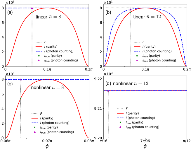
Figure 7: CFI and QFI for parity and photon-counting measurements in the case of both linear and nonlinear cases with different values of average photon number. (a) and (b) show the results of the linear case with $\bar{n}=8$ and $\bar{n}=12$, respectively. (c) and (d) show the results of the nonlinear case with $\bar{n}=8$ and $\bar{n}=12$, respectively. The dotted black line, solid red line, and dashed blue line represent the QFI, the CFI for parity measurement, and the CFI for photon-counting measurement, respectively. The Fock space dimension is $11$ $(N=10)$.

The optimality of the parity and photon-counting measurement usually relies on the true value of $\phi$. As shown in Fig. 7, in the linear case with $\bar{n}=8,12$, the CFI with respect to the parity (solid red line) and photon-counting measurement (dashed blue line) can only reach the QFI (dotted black line) at some specific value of $\phi$. A similar phenomenon occurs in the nonlinear case with $\bar{n}=8$. In the nonlinear case with $\bar{n}=12$, both parity and photon-counting measurements are optimal for all values of $\phi$.

To overcome the dependence of optimality on the true value, adaptive measurement has to be involved. In the adaptive measurement, a tunable phase $\phi_{\mathrm{u}}$ is included in mode $a$, and the total phase difference now becomes $\phi+\phi_{\mathrm{u}}$. In each round of the measurement, parity or photon-counting measurements are performed and a new value of $\phi_{u}$ is calculated and used in the next round. The specific process of adaptive measurement and corresponding thorough calculations can be found in a recent review [63].

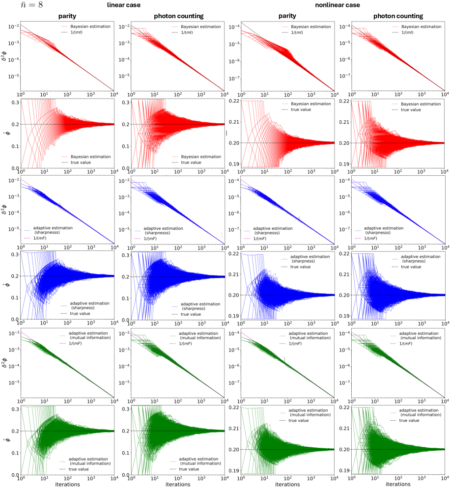
Figure 8: Performance of $\hat{\phi}$ and $\delta^{2}\phi$ of 2000 rounds simulations for the adaptive measurement in the case of $\bar{n}=8$. The true value of $\phi$ is taken as 0.2. The Fock space dimension is $11$ $(N=10)$.

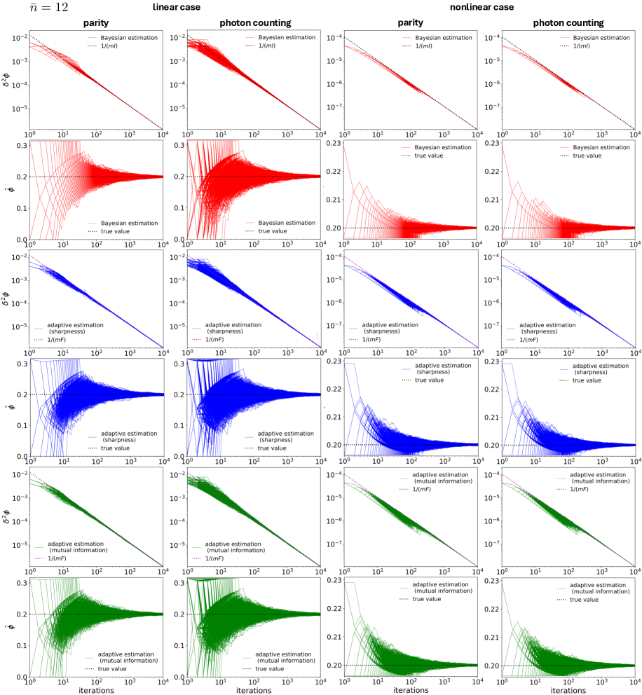
Figure 9: Performance of $\hat{\phi}$ and $\delta^{2}\phi$ of 2000 rounds simulations for the adaptive measurement in the case of $\bar{n}=12$. The true value of $\phi$ is taken as 0.2. The Fock space dimension is $11$ $(N=10)$.

In this paper, we use the average sharpness functions [55, 56, 57, 54, 58, 59, 60, 61] and mutual information [59, 60, 61, 62, 65] as the objective function to update $\phi_{\mathrm{u}}$. The sharpness function in the $(k+1)$th round of iteration can be expressed by [55, 56]

$$S_{k+1}(\phi_{\mathrm{u}})=\frac{\left|\int^{2\pi}_{0}P(y|\phi,\phi_{\mathrm{u}})P_{k+1}(\phi)e^{i\phi}d\phi\right|}{\int^{2\pi}_{0}P(y|\phi,\phi_{\mathrm{u}})P_{k+1}(\phi)d\phi},$$ (167)

where $P_{k+1}(\phi)$ is the prior probability in $(k+1)$th round. It is updated via the Bayes’ rule, namely, it is taken as the posterior distribution $P_{k}(\phi|y,\phi_{{\mathrm{u}},k-1})$ obtained in $k$th round. According to the Bayes’ theorem, the posterior distribution can be expressed by

$$P_{k}(\phi|y,\phi_{{\mathrm{u}},k-1})=\frac{P(y|\phi,\phi_{{\mathrm{u}},k-1})P_{k}(\phi)}{\int^{2\pi}_{0}P(y|\phi,\phi_{{\mathrm{u}},k-1})P_{k}(\phi)d\phi},$$ (168)

where $\phi_{{\mathrm{u}},k-1}$ is the value of $\phi_{\mathrm{u}}$ obtained in the $(k-1)$th round and used in the $k$th round. $P_{k}(\phi)$ is the prior distribution in the $k$th round. $P(y|\phi,\phi_{{\mathrm{u}},k-1})$ is the conditional probability for the result $y$. For parity measurement, in the linear case $P(y|\phi,\phi_{{\mathrm{u}},k-1})$ is in the forms of Eqs. (118) and (119) when $\bar{n}\leq N$, and in the forms of Eqs. (126) and (127) when $\bar{n}\geq N$. In the nonlinear case, it takes the form of Eqs. (136) and (137) when $\bar{n}\leq N$, and Eq. (144) when $\bar{n}\geq N$. For the measurement of photon counting, it takes the form of Eqs. (149) and (153) in the linear case, and Eqs. (158) and (161) in the nonlinear case. For the formulas of conditional probability mentioned above, $\phi$ in the formulas should be replaced with $\phi+\phi_{\mathrm{u}}$.

An alternative choice of sharpness is replacing $\exp(i\phi)$ in Eq. (167) with $\exp(i2\pi\phi/T)$, as done in Refs. [56, 57, 58]. Here $T$ is the period of the conditional probability. However, the performance of the adaptive measurement has no significant difference for these two formulas according to our test. Hence, in this paper we use Eq. (167) as the objective function.

In the $(k+1)$th round, the value of $\phi_{\mathrm{u}}$ (denoted by $\phi_{{\mathrm{u}},k+1}$) is taken as the argument that can maximize the average sharpness,

$$\phi_{{\mathrm{u}},k+1}\!=\!\mathrm{argmax}\,\sum_{y}\left|\int^{2\pi}_{0}e^{i\phi}P(y|\phi,\phi_{{\mathrm{u}}})P_{k+1}(\phi)d\phi\right|.$$ (169)

Apart from the sharpness function, the mutual information can also be used as the objective function for the update of $\phi_{\mathrm{u}}$. In our case, the average mutual information in the $(k+1)$th round of iteration can be expressed by [59, 72]

$$\mathcal{I}_{k+1}(\phi_{\mathrm{u}})= \sum_{y}\int^{2\pi}_{0}d\phi\,P(y|\phi,\phi_{{\mathrm{u}}})P_{k+1}(\phi)$$

$$\times\log_{2}\left[\frac{P(y|\phi,\phi_{{\mathrm{u}}})}{\int^{2\pi}_{0}P(y|\phi,\phi_{{\mathrm{u}}})P_{k+1}(\phi)d\phi}\right].$$ (170)

The value of $\phi_{\mathrm{u}}$ in the $(k+1)$th round is taken as

$$\phi_{{\mathrm{u}},k+1}=\mathrm{argmax}\leavevmode\nobreak\ \mathcal{I}_{k+1}(\phi_{\mathrm{u}}).$$ (171)

In this paper, the experimental results are simulated via a random number $s\in[0,1]$. The regime $[0,1]$ is separated into $m$ parts according to the distribution of the conditional probability. Here $m$ is the number of measurement results. The width of the $k$th ($k=1,2,\dots,m$) regime is equivalent to the value of the conditional probability for the $k$th result. In one round of the simulation, a random value of $s$ is generated, and if this value is located in the $k$th regime, then the $k$th result is then taken as the simulated experimental result.

The classical estimation in this paper is finished by the maximum a posterior method, namely, the estimated value $\hat{\phi}$ in the $k$th round is obtained via the following equation

$$\hat{\phi}_{k}=\mathrm{argmax}\leavevmode\nobreak\ P_{k}(\phi|y,\phi_{{\mathrm{u}},k-1}).$$ (172)

The variance $\delta^{2}\phi$ in the $k$th round can be calculated by

$$\delta^{2}\phi= \int\phi^{2}P_{k}(\phi|y,\phi_{{\mathrm{u}},k-1})d\phi$$

$$-\left(\int\phi P_{k}(\phi|y,\phi_{{\mathrm{u}},k-1})d\phi\right)^{2}.$$ (173)

For both parity and photon-counting measurements, the conditional probabilities are periodic according to Eqs. (126), (127), (136), (137), and (144). In one period, two peaks exist and the Bayesian estimation cannot pick the right one, which will cause a wrong estimation. To avoid this problem, the prior distribution is taken as half of the period in this paper. For the sake of a fair performance comparison, the prior distribution in the adaptive measurement is taken as the same one as the Bayesian estimation. Specifically to say, the prior distribution in the demonstration is taken as a uniform distribution in the regime $[0,\pi/10]$ for all examples in the linear case. In the nonlinear case, the prior distribution is taken as a uniform distribution in the regime $\left[3\pi/50,7\pi/100\right]$ for $\bar{n}=8$, and $\left[\pi/16,7\pi/96\right]$ for $\bar{n}=12$.

In the adaptive measurement, the true value of $\phi$ in all examples is taken as $0.2$. The corresponding values of CFI are illustrated in Fig. 7. $2000$ rounds of experiments are simulated and the corresponding performance of $\hat{\phi}$ and $\delta^{2}\phi$ are shown in Fig. 8 for $\bar{n}=8$ and Fig. 9 for $\bar{n}=12$. The average performance of $2000$ rounds is given in the main text. The true values of $\phi$ in these figures are taken as $0.2$.

Appendix H Calculations under the noise of photon loss

H.1 Expressions of the reduced density matrices

The photon loss in the MZI can be modeled by the fictitious beam splitters [66, 67, 67, 68, 69, 40, 41, 70, 42, 71], which can be expressed by

$$B_{ac} = e^{i\frac{\eta_{1}}{2}\left(a^{{\dagger}}c+ac^{{\dagger}}\right)},$$ (174)

$$B_{bd} = e^{i\frac{\eta_{2}}{2}\left(b^{{\dagger}}d+bd^{{\dagger}}\right)},$$ (175)

where $c$ and $d$ are two fictitious modes representing the photon loss. The transmission coefficients for these two beam splitters are $T_{1}=\cos^{2}(\eta_{1}/2)$ and $T_{2}=\cos^{2}(\eta_{2}/2)$. When $T_{1}=1$ ($T_{2}=1$), no photon leaks from $c$ ($d$) mode, and when $T_{1}=0$ ($T_{2}$=0), all photons leak from $c$ ($d$) mode. As a matter of fact, these two fictitious beam splitters can be placed either in front of or behind the phase shifts, which would not cause different results [69, 40].

Taking into account the fictitious modes $c$ and $d$, the total probe state can be written as

$$\ket{\psi_{\mathrm{tot}}}=\ket{\psi_{\mathrm{opt}}}\ket{0}_{c}\ket{0}_{d}.$$ (176)

After going through the fictitious beam splitters, the state becomes mixed and the corresponding density matrix can be expressed by

$$\rho=\mathrm{Tr}_{cd}\left(B_{bd}B_{ac}\ket{\psi_{\mathrm{tot}}}\bra{\psi_{\mathrm{tot}}}{B^{{\dagger}}_{ac}}{B^{{\dagger}}_{bd}}\right),$$ (177)

where $\mathrm{Tr}_{cd}(\cdot)$ is the partial trace on the modes $c$ and $d$. Notice that $\ket{\psi_{\mathrm{opt}}}$ already includes the influence of the first beam splitter, if there is one. The state above is actually the state before going through the phase shifts.

Now let us first consider the optimal state for $\bar{n}\leq N$ in the linear case, which is

$$\sqrt{\frac{N-\bar{n}}{N}}\ket{00}+\sqrt{\frac{\bar{n}}{2N}}\left(e^{i\theta_{1}}\ket{0N}+e^{i\theta_{2}}\ket{N0}\right).$$ (178)

Utilizing the equations

$$e^{i\frac{\eta_{1}}{2}(a^{{\dagger}}c+ac^{{\dagger}})}\ket{N0}\ket{0}_{c}\ket{0}_{d}$$

$$= \sum_{k=0}^{N}\binom{N}{k}^{\frac{1}{2}}i^{k}T_{1}^{\frac{1}{2}(N-k)}R_{1}^{\frac{k}{2}}\ket{N-k,0}\ket{k}_{c}\ket{0}_{d},$$ (179)

and

$$e^{i\frac{\eta_{2}}{2}(b^{{\dagger}}d+bd^{{\dagger}})}\ket{0N}\ket{0}_{c}\ket{0}_{d}$$

$$= \sum_{k=0}^{N}\binom{N}{k}^{\frac{1}{2}}\!\!i^{k}T_{2}^{\frac{1}{2}(N-k)}R_{2}^{\frac{k}{2}}\ket{0,N-k}\ket{0}_{c}\ket{k}_{d},$$ (180)

where $R_{1(2)}=1-T_{1(2)}$, the reduced density matrix can be expressed by

$$\rho= \frac{N-\bar{n}}{N}\ket{00}\bra{00}+\sqrt{\frac{\bar{n}(N-\bar{n})}{2N^{2}}}\rho_{1}$$

$$+\frac{\bar{n}}{2N}\sum_{k=0}^{N}\binom{N}{k}\rho_{2,k}+\frac{\bar{n}}{2N}\rho_{3},$$ (181)

where

$$\rho_{1} = T_{1}^{\frac{N}{2}}\left(e^{-i\theta_{2}}\ket{00}\bra{N0}+e^{i\theta_{2}}\ket{N0}\bra{00}\right)$$ (182)

$$+T_{2}^{\frac{N}{2}}\left(e^{-i\theta_{1}}\ket{00}\bra{0N}+e^{i\theta_{1}}\ket{0N}\bra{00}\right),$$

and

$$\rho_{2,k} = T_{1}^{N-k}R_{1}^{k}\ket{N-k,0}\bra{N-k,0}$$ (183)

$$+T_{2}^{N-k}R_{2}^{k}\ket{0,N-k}\bra{0,N-k},$$

and

$$\rho_{3}=\left(T_{1}T_{2}\right)^{\frac{N}{2}}\left[e^{i(\theta_{1}-\theta_{2})}\ket{0N}\bra{N0}+e^{i(\theta_{2}-\theta_{1})}\ket{N0}\bra{0N}\right].$$ (184)

In the linear case with $\bar{n}\geq N$, the optimal state reads

$$\sqrt{\frac{2N-\bar{n}}{2N}}\left(e^{i\theta_{1}}\ket{0N}+e^{i\theta_{2}}\ket{N0}\right)+\sqrt{\frac{\bar{n}-N}{N}}\ket{NN}.$$ (185)

Then the reduced density matrix can be written as

$$\rho= \frac{2N-\bar{n}}{2N}\left[\sum_{k=0}^{N}\binom{N}{k}\rho_{2,k}+\rho_{3}\right]$$

$$+\sqrt{\frac{(2N-\bar{n})(\bar{n}-N)}{2N^{2}}}\sum_{k=0}^{N}\binom{N}{k}\left(\rho_{4,k}+\rho_{5,k}\right)$$

$$+\frac{\bar{n}-N}{N}\!\!\sum_{k,l=0}^{N}\!\!\binom{N}{k}\!\binom{N}{l}\rho_{6,kl},$$ (186)

where

$$\rho_{4,k} = T_{2}^{N-k}R_{2}^{k}T_{1}^{\frac{N}{2}}\left(e^{i\theta_{1}}\ket{0,N-k}\bra{N,N-k}\right.$$ (187)

$$\left.+e^{-i\theta_{1}}\ket{N,N-k}\bra{0,N-k}\right),$$

and

$$\rho_{5,k} = T_{1}^{N-k}R_{1}^{k}T_{2}^{\frac{N}{2}}\left(e^{i\theta_{2}}\ket{N-k,0}\bra{N-k,N}\right.$$ (188)

$$\left.+e^{-i\theta_{2}}\ket{N-k,N}\bra{N-k,0}\right),$$

and

$$\rho_{6,kl}=T_{1}^{N-k}R_{1}^{k}T_{2}^{N-l}R_{2}^{l}\ket{N-k,N-l}\bra{N-k,N-l}.$$ (189)

In the nonlinear case, the optimal state is the same as the counterpart in the linear case when $\bar{n}\leq N$, thus, the corresponding reduced density matrix is also in the form of Eq. (181). When $\bar{n}\geq N$, we consider a simple case of the optimal state

$$\frac{1}{\sqrt{2}}\left(\ket{\bar{n}-N,N}+e^{i\theta}\ket{N,\bar{n}-N}\right)$$ (190)

with $\bar{n}$ an integer in the regime $[N,4N/3]$. In this case, the reduced density matrix reads

$$\rho= \frac{1}{2}\sum_{k=0}^{\bar{n}-N}\sum_{l=0}^{N}\binom{\bar{n}-N}{k}\binom{N}{l}\rho_{7,kl}$$

$$+\frac{1}{2}\sum_{k,l=0}^{\bar{n}-N}\binom{\bar{n}-N}{k}^{\frac{1}{2}}\binom{N}{k}^{\frac{1}{2}}\binom{\bar{n}-N}{l}^{\frac{1}{2}}\binom{N}{l}^{\frac{1}{2}}\rho_{8,kl},$$ (191)

where

$$\rho_{7,kl}$$ (192)

$$= T_{1}^{\bar{n}-N-k}R_{1}^{k}T_{2}^{N-l}R_{2}^{l}$$

$$\times\ket{\bar{n}-N-k,N-l}\bra{\bar{n}-N-k,N-l}$$

$$+T_{1}^{N-l}R_{1}^{l}T_{2}^{\bar{n}-N-k}R_{2}^{k}$$

$$\times\ket{N-l,\bar{n}-N-k}\!\bra{N-l,\bar{n}-N-k},$$

and

$$\rho_{8,kl}$$ (193)

$$= T_{1}^{\frac{\bar{n}}{2}-k}R_{1}^{k}T_{2}^{\frac{\bar{n}}{2}-l}R_{2}^{l}$$

$$\times\left(e^{-i\theta}\!\ket{\bar{n}\!-\!N\!-\!k,N\!-\!l}\!\bra{N\!-\!k,\bar{n}\!-\!N\!-\!l}\right.$$

$$\left.+e^{i\theta}\ket{N\!-\!k,\bar{n}\!-\!N\!-\!l}\bra{\bar{n}\!-\!N\!-\!k,N\!-\!l}\right)\!.$$

The QFIs for these reduced density matrices are calculated numerically via QuanEstimation [61].

H.2 Conditional probabilities for parity and photon-counting measurements

In this section, we provide the expression of the conditional probability for parity and photon-counting measurements in both linear and nonlinear cases.

H.2.1 Parity measurement

We first discuss the linear case. When the photon loss exists, the state before going through the phase shifts is in the form of Eq. (181), thus, the expectation of the parity operator reads

$$\expectationvalue{\Pi_{a}} =\mathrm{Tr}\left(\Pi_{a}e^{i\frac{\pi}{2}J_{x}}e^{i\phi J_{z}}\rho e^{-i\phi J_{z}}e^{-i\frac{\pi}{2}J_{x}}\right)$$

$$=\mathrm{Tr}\left(e^{i\frac{\pi}{2}n}e^{-i\pi J_{y}}e^{i\phi J_{z}}\rho e^{-i\phi J_{z}}\right)$$

$$=1-\frac{\bar{n}}{N}\left[1-\left(T_{1}T_{2}\right)^{\frac{N}{2}}\cos\beta_{1}\right],$$ (194)

where $\beta_{1}$ is given by Eq. (111). According to the conditions $\expectationvalue{\Pi_{a}}=P_{+}-P_{-}$ and $P_{+}+P_{-}=1$, the probability can be calculated as

$$P_{+} =1-\frac{\bar{n}}{2N}\left[1-\left(T_{1}T_{2}\right)^{\frac{N}{2}}\cos\beta_{1}\right],$$ (195)

$$P_{-} =\frac{\bar{n}}{2N}\left[1-\left(T_{1}T_{2}\right)^{\frac{N}{2}}\cos\beta_{1}\right],$$ (196)

and the CFI can be written as

$$\frac{\bar{n}N^{2}\left(T_{1}T_{2}\right)^{N}\sin^{2}\beta_{1}}{\left[\!1\!-\!\left(T_{1}T_{2}\right)^{\frac{N}{2}}\!\cos\beta_{1}\!\right]\!\!\left\{2N\!-\!\bar{n}\!\left[\!1-\left(T_{1}T_{2}\right)^{\frac{N}{2}}\!\cos\beta_{1}\!\right]\!\right\}}.$$ (197)

Based on the expression above, the maximum CFI with respect to $\beta_{1}$ reads

$$I_{\max}=\bar{n}N\!-\!\frac{1}{2}\bar{n}\left\{\Omega\bar{n}\!+\!\sqrt{\Omega\left[4N(N\!-\!\bar{n})+\bar{n}^{2}\Omega\right]}\right\},$$ (198)

where

$$\Omega:=1-(T_{1}T_{2})^{N}.$$ (199)

$I_{\max}$ can be attained when $\cos\beta_{1}=0$ for $\bar{n}=N$, and

$$\cos\beta_{1}=\frac{2(N-\bar{n})+\Omega\bar{n}-\sqrt{\Omega\left[\Omega\bar{n}^{2}+4N(N-\bar{n})\right]}}{2(N-\bar{n})\sqrt{1-\Omega}}$$ (200)

for $\bar{n}<N$. Then the optimal points of the true values of $\phi$ can be located accordingly.

In the case that $\bar{n}\geq N$, the reduced density matrix is in the form of Eq. (186), and the expectation of $\Pi_{a}$ is

$$\expectationvalue{\Pi_{a}}=\frac{\bar{n}}{N}-1+\left(2-\frac{\bar{n}}{N}\right)\left(T_{1}T_{2}\right)^{\frac{N}{2}}\!\cos\beta_{1},$$ (201)

which further gives the expressions of $P_{+}$ and $P_{-}$ as follows:

$$P_{+} =1-\left(1-\frac{\bar{n}}{2N}\right)\left[1-\left(T_{1}T_{2}\right)^{\frac{N}{2}}\cos\beta_{1}\right],$$

$$P_{-} =\left(1-\frac{\bar{n}}{2N}\right)\left[1-\left(T_{1}T_{2}\right)^{\frac{N}{2}}\cos\beta_{1}\right].$$ (202)

The CFI then reads

$$\frac{(2N-\bar{n})N^{2}\left(T_{1}T_{2}\right)^{N}\sin^{2}\beta_{1}}{\left[\!1\!-\!(T_{1}T_{2})^{\frac{N}{2}}\cos\beta_{1}\!\right]\!\!\left\{\!2N\!-\!(2N\!-\!\bar{n})\!\left[\!1\!-\!(T_{1}T_{2})^{\frac{N}{2}}\cos\beta_{1}\right]\!\right\}}.$$ (203)

The maximum CFI with respect to $\beta_{1}$ reads

$$I_{\max}= (2N-\bar{n})N-\frac{1}{2}(2N-\bar{n})$$

$$\times\left[(2N\!-\!\bar{n})\Omega\!+\!\sqrt{\Omega\left[\Omega(2N\!-\!\bar{n})^{2}\!+\!4N(\bar{n}\!-\!N)\right]}\right].$$ (204)

Here $\Omega$ is defined in Eq. (199). $I_{\max}$ can be attained when $\cos\beta_{1}=0$ for $\bar{n}=N$, and

$$\cos\beta_{1}=\sqrt{1-\Omega}-\frac{\Omega\bar{n}\!-\!\sqrt{\Omega\left[\Omega(2N\!-\!\bar{n})^{2}\!+\!4N(\bar{n}\!-\!N)\right]}}{2(N-\bar{n})\sqrt{1-\Omega}}$$ (205)

for $\bar{n}>N$. Then the optimal points of the true values of $\phi$ can be located accordingly.

In the nonlinear case, the reduced density matrix is given by Eq. (186) when $\bar{n}\leq N$. For this state, the expectation of the parity operator is

$$\expectationvalue{\Pi_{a}}=1-\frac{\bar{n}}{N}\left[1-(T_{1}T_{2})^{\frac{N}{2}}\cos\beta_{2}\right],$$ (206)

where $\beta_{2}$ is given by Eq. (132). The corresponding probabilities $P_{\pm}$ are

$$P_{+} =1-\frac{\bar{n}}{2N}\left[1-(T_{1}T_{2})^{\frac{N}{2}}\cos\beta_{2}\right],$$ (207)

$$P_{-} =\frac{\bar{n}}{2N}\left[1-(T_{1}T_{2})^{\frac{N}{2}}\cos\beta_{2}\right].$$ (208)

The CFI is

$$\frac{\bar{n}N^{4}(T_{1}T_{2})^{N}\sin^{2}\beta_{2}}{\left[1-\!(T_{1}T_{2})^{\frac{N}{2}}\!\cos\beta_{2}\right]\!\!\left\{2N\!-\!\bar{n}\!\left[1\!-\!(T_{1}T_{2})^{\frac{N}{2}}\!\cos\beta_{2}\right]\!\right\}}.$$ (209)

In this case, the maximum CFI with respect to $\beta_{2}$ is

$$I_{\max}=\bar{n}N^{3}\!-\!\frac{1}{2}\bar{n}N^{2}\left(\bar{n}\Omega\!+\!\sqrt{\Omega\left[4N(N\!-\!\bar{n})+\bar{n}^{2}\Omega\right]}\right),$$ (210)

where $\Omega$ is defined in Eq. (199). $I_{\max}$ can be attained when $\cos\beta_{2}=0$ for $\bar{n}=N$, and

$$\cos\beta_{2}=\frac{2(N\!-\!\bar{n})\!+\!\Omega\bar{n}\!-\!\sqrt{\Omega\left[\Omega\bar{n}^{2}+4N(N-\bar{n})\right]}}{2(N-\bar{n})\sqrt{1-\Omega}}$$ (211)

for $\bar{n}<N$. Then the optimal points of the true values of $\phi$ can be located accordingly.

In the case that $\bar{n}\geq N$, we also consider the simple case that $\bar{n}$ is an integer in the regime $[N,4N/3]$. The corresponding reduced density matrix is given in Eq. (191). For this state, the value of $\expectationvalue{\Pi_{a}}$ reads

$$\expectationvalue{\Pi_{a}}= \sum^{\bar{n}-N}_{k=0}\binom{\bar{n}-N}{k}\binom{N}{k}(T_{1}T_{2})^{\frac{\bar{n}}{2}-k}(R_{1}R_{2})^{k}\cos\gamma_{k}$$

$$+\frac{1}{2}\sum^{\bar{n}-N}_{k=0}\binom{\bar{n}-N}{k}\binom{N}{\bar{n}-N-k}(T_{1}T_{2})^{\bar{n}-N-k}$$

$$\times(R_{1}R_{2})^{k}\left(R^{2N-\bar{n}}_{1}+R^{2N-\bar{n}}_{2}\right),$$ (212)

where $\gamma_{k}:=\gamma-2k(2N-\bar{n})\phi$ with $\gamma$ given by Eq. (142). $P_{\pm}=(1\pm\expectationvalue{\Pi_{a}})/2$ can be calculated via the equation above correspondingly.

With all the expressions of the conditional probabilities, the adaptive measurement can be performed and simulated.

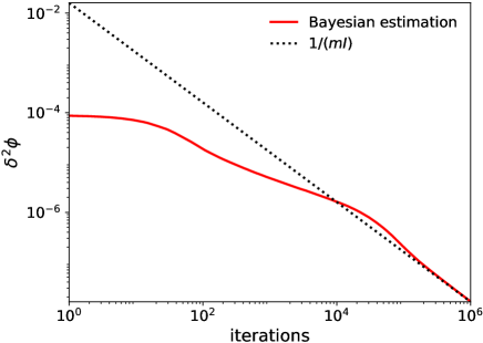
Figure 10: Noisy performance of Bayesian estimation for parity measurement in the nonlinear case. The average photon number $\bar{n}=12$, the Fock space dimension is taken as $11$ ($N=10$). The transmission rates $T_{1}=T_{2}=0.9$.

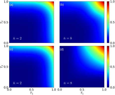
Figure 11: Noisy behaviors of the QFI as a function of $T_{1}$ and $T_{2}$ in the case of (a) linear phase shift with $\bar{n}<N$ ($\bar{n}=2$), (b) linear phase shift with $\bar{n}>N$ ($\bar{n}=8$), (c) nonlinear phase shift with $\bar{n}<N$ ($\bar{n}=2$), and (d) nonlinear phase shift with $\bar{n}>N$ ($\bar{n}=8$). The Fock space dimension is taken as $7$ ($N=6$).

H.2.2 Photon-counting measurement

Here we provide the expressions of the conditional probabilities for the photon-counting measurement in the case that photon loss exists. Recall that the reduced density matrix before going through the phase shifts is given in Eq. (181) for $\bar{n}\leq N$. Then the probability $P_{m}$ is

$$P_{m}= \mathrm{Tr}\left(e^{i\phi J_{z}}\rho e^{-i\phi J_{z}}e^{-i\frac{\pi}{2}J_{x}}\sum^{2N}_{j=0}\ket{mj}\bra{mj}e^{i\frac{\pi}{2}J_{x}}\right).$$

$$= \left(1-\frac{\bar{n}}{N}\right)\delta_{0m}+\frac{\bar{n}}{N}\Lambda+h(m-N)2^{-N}\frac{\bar{n}}{N}$$

$$\times\binom{N}{m}\left(T_{1}T_{2}\right)^{\frac{N}{2}}(-1)^{m}\cos\beta_{1},$$ (213)

where $h(m-N)$ is the step function defined in Eq. (150), and $\Lambda$ is defined by

$$\Lambda:=\sum^{N-m}_{k=0}2^{k\!-\!N\!-\!1}\binom{N}{k}\!\binom{N\!-\!k}{m}\left(T^{N-k}_{1}R^{k}_{1}\!+\!T^{N-k}_{2}R^{k}_{2}\right).$$ (214)

In the case that $\bar{n}\geq N$, the reduced density matrix is in the form of Eq. (186), and $P_{m}$ then reads

$$P_{m}$$

$$= \left(2-\frac{\bar{n}}{N}\right)\Lambda+h(m-N)\left(2-\frac{\bar{n}}{N}\right)2^{-N}(-1)^{m}$$

$$\times\binom{N}{m}(T_{1}T_{2})^{\frac{N}{2}}\cos\beta_{1}+2^{-2N}\left(\frac{\bar{n}}{N}-1\right)$$

$$\times\!\sum^{N}_{k,l=0}\!2^{k+l}\frac{m!(2N-m-k-l)!}{(N-k)!(N-l)!}\binom{N}{k}\binom{N}{l}T^{N-k}_{1}R^{k}_{1}$$

$$\times\!T^{N-l}_{2}R^{l}_{2}\!\!\left[\!\sum^{\min\{N-k,m\}}_{s=\max\{0,m-N+l\}}\!\!\!\!(-1)^{s}\binom{N\!-\!k}{s}\!\binom{N\!-\!l}{m\!-\!s}\!\!\right]^{2}\!\!\!.$$ (215)

In the nonlinear case, the reduced density matrix is the same as that in the linear case for $\bar{n}\leq N$, namely, Eq. (181). The probability $P_{m}$ is then calculated as

$$P_{m}= \left(1-\frac{\bar{n}}{N}\right)\delta_{0m}+\frac{\bar{n}}{N}\Lambda+h(m-N)2^{-N}\frac{\bar{n}}{N}$$

$$\times\binom{N}{m}(T_{1}T_{2})^{\frac{N}{2}}(-1)^{m}\cos\beta_{2}.$$ (216)

When $\bar{n}\geq N$, the reduced density matrix is in the form of Eq. (191) for the simple case that $\bar{n}$ is an integer in the regime $[N,4N/3]$. Hence, the probability can be expressed by

$$P_{m}= \sum^{\bar{n}-N}_{k=0}\sum^{N}_{l=0}2^{k+l-\bar{n}-1}\frac{m!(\bar{n}\!-\!m\!-\!k\!-\!l)!}{(\bar{n}\!-\!N\!-\!k)!(N\!-\!l)!}\binom{\bar{n}\!-\!N}{k}\!\binom{N}{l}$$

$$\!\times\!\!\left[\sum^{\min\{N-l,m\}}_{s=\max\{0,N+m-\bar{n}+k\}}\!\!\!(-1)^{s}\binom{N-l}{s}\binom{\bar{n}\!-\!N\!-\!k}{m\!-\!s}\!\right]^{2}$$

$$\times\!\!\left(T^{\bar{n}-N-k}_{1}R^{k}_{1}T^{N-l}_{2}R^{l}_{2}+T^{N-l}_{1}R^{l}_{1}\!T^{\bar{n}-N-k}_{2}R^{k}_{2}\right)$$

$$+\sum^{\bar{n}-N}_{k,l=0}\!\!2^{k+l-\bar{n}}\frac{m!(\bar{n}-m-k-l)!k!l!}{(\bar{n}-N)!N!}\binom{\bar{n}-N}{k}$$

$$\times\!\binom{N}{k}\!\binom{\bar{n}-N}{l}\!\binom{N}{l}T^{\frac{\bar{n}}{2}-k}_{1}R^{k}_{1}T^{\frac{\bar{n}}{2}-l}_{2}R^{l}_{2}$$

$$\times\cos\left(\gamma-(k+l)(2N-\bar{n})\phi\right)$$

$$\times\sum^{\min\{\bar{n}-N-l,m\}}_{s=\max\{0,m-N+k\}}\sum^{\min\{N-l,m\}}_{t=\max\{0,N+m-\bar{n}+k\}}\!\!\!(-1)^{s+t}$$

$$\times\!\binom{\bar{n}-N-l}{s}\!\binom{N-k}{m-s}\!\binom{\bar{n}-N-k}{m-t}\!\binom{N-l}{t}$$ (217)

for $m\leq\bar{n}$ and zero for $m>\bar{n}$.

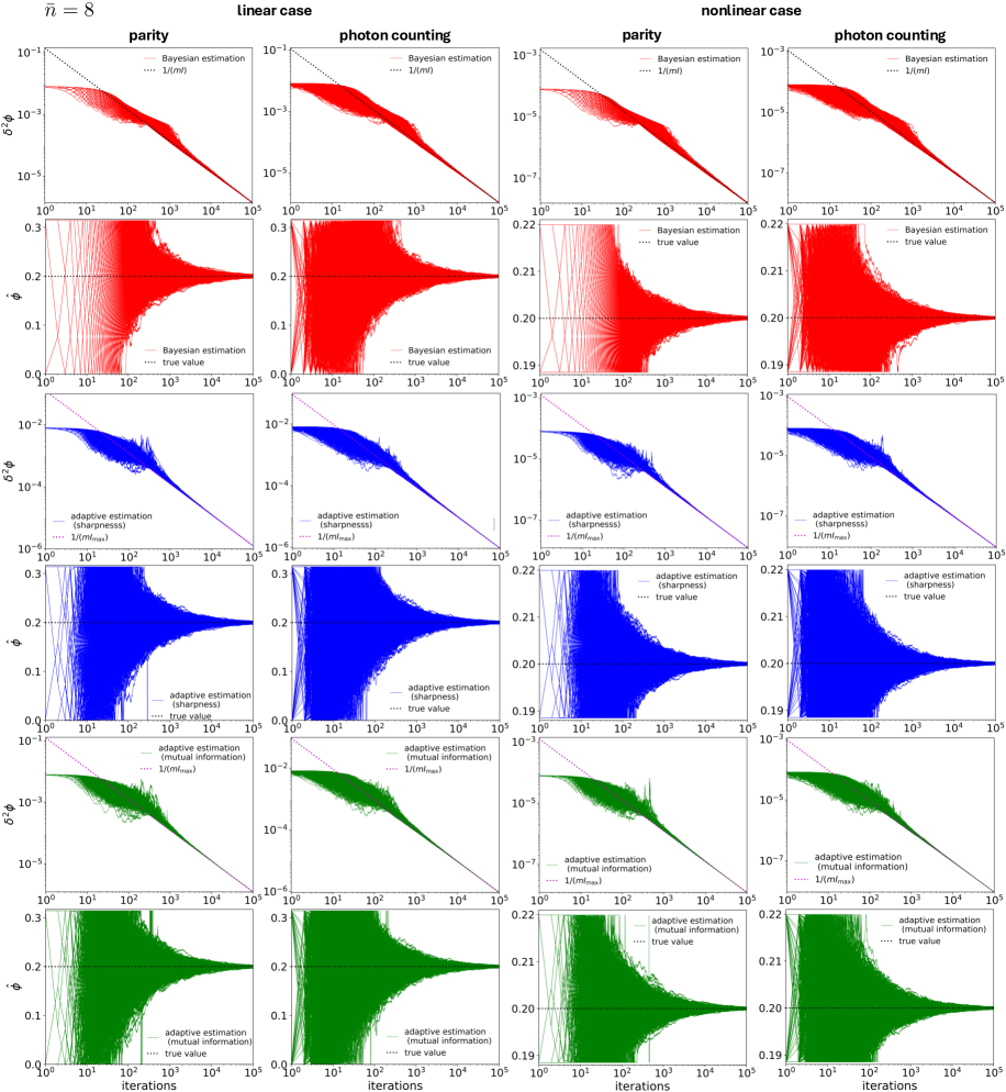
Figure 12: Noisy performance of $\hat{\phi}$ and $\delta^{2}\phi$ of 2000 rounds simulations for the adaptive measurement in the case of $\bar{n}=8$. The true value of $\phi$ is taken as $0.2$. The transmission rates are taken as $T_{1}=T_{2}=0.9$. The Fock space dimension is $11$ $(N=10)$.

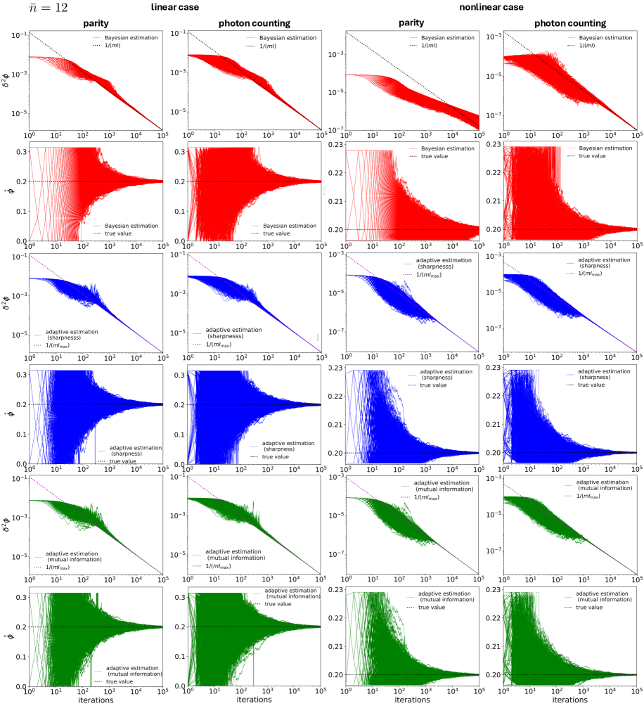
Figure 13: Noisy performance of $\hat{\phi}$ and $\delta^{2}\phi$ of 2000 rounds simulations for the adaptive measurement in the case of $\bar{n}=12$. The true value of $\phi$ is taken as $0.2$. The transmission rates are taken as $T_{1}=T_{2}=0.9$. The Fock space dimension is $11$ $(N=10)$.

The CFIs for these conditional probabilities are calculated numerically via QuanEstimation [61]. The average performance of Bayesian estimation for parity measurement in the nonlinear case under noise is given in Fig. 10. The convergence speed is significantly lower than that in the noiseless case, which is reasonable since the actually used photons in the estimation are less than the noiseless case in the same time duration.

Moreover, the noisy behaviors of the QFI as a function of $T_{1}$ and $T_{2}$ have been illustrated in Fig. 11 for both linear and nonlinear phase shifts. In each plot, the area proportion of the ratio $F_{\mathrm{loss}}/F$ that is larger than a given threshold is used to reflect the robustness. Here $F_{\mathrm{loss}}$ and $F$ are the QFI for the optimal states with and without loss, respectively. In this paper, two values of the threshold, 0.6 and 0.8, are used to make sure that the result does not rely on the choice of this value.

With all the aforementioned expressions of the conditional probabilities, the adaptive measurement can be performed and simulated. 2000 rounds of experiments are simulated and the corresponding performance of $\hat{\phi}$ and $\delta^{2}\phi$ are shown in Fig. 12 for $\bar{n}=8$ and Fig. 13 for $\bar{n}=12$. The average performance of 2000 rounds is given in the main text. The true values of $\phi$ in these figures are taken as $0.2$, and the transmission rates are taken as $T_{1}=T_{2}=0.9$.

References

• [1] C. M. Caves, Quantum-mechanical noise in an interferometer, Phys. Rev. D 23, 1693 (1981).
• [2] C. M. Caves, Quantum limits on noise in linear amplifiers, Phys. Rev. D 26, 1817 (1982).
• [3] M. J. Holland and K. Burnett, Interferometric Detection of Optical Phase Shifts at the Heisenberg Limit, Phys. Rev. Lett. 71, 1355 (1993).
• [4] V. Giovannetti, S. Lloyd, and L. Maccone, Quantum-Enhanced Measurements: Beating the Standard Quantum Limit, Science 306, 1330 (2004).
• [5] V. Giovannetti, S. Lloyd, and L. Maccone, Quantum Metrology, Phys. Rev. Lett. 96, 010401 (2006).
• [6] A. Monras and M. G. A. Paris, Optimal Quantum Estimation of Loss in Bosonic Channels, Phys. Rev. Lett. 98, 160401 (2007).
• [7] L. Pezzé, A. Smerzi, G. Khoury, J. F. Hodelin, and D. Bouwmeester, Phase Detection at the Quantum Limit with Multiphoton Mach-Zehnder Interferometry, Phys. Rev. Lett. 99, 223602 (2007).
• [8] L. Pezzé and A. Smerzi, Mach-Zehnder Interferometry at the Heisenberg Limit with Coherent and Squeezed-Vacuum Light, Phys. Rev. Lett. 100, 073601 (2008).
• [9] S. Boixo, A. Datta, M. J. Davis, S. T. Flammia, A. Shaji, and C. M. Caves, Quantum Metrology: Dynamics versus Entanglement, Phys. Rev. Lett. 101, 040403 (2008).
• [10] L. Pezzé and A. Smerzi, Entanglement, Nonlinear Dynamics, and the Heisenberg Limit, Phys. Rev. Lett. 102, 100401 (2009).
• [11] M. G. A. Paris, Quantum estimation for quantum technology, Int. J. Quantum Inf. 7, 125 (2009).
• [12] M. G. Genoni, S. Olivares, and M. G. A. Paris, Optical Phase Estimation in the Presence of Phase Diffusion, Phys. Rev. Lett. 106, 153603 (2011).
• [13] N. Thomas-Peter, B. J. Smith, A. Datta, L. Zhang, U. Dorner, and I. A. Walmsley, Real-World Quantum Sensors: Evaluating Resources for Precision Measurement, Phys. Rev. Lett. 107, 113603 (2011).
• [14] N. Spagnolo, C. Vitelli, V. G. Lucivero, V. Giovannetti, L. Maccone, and F. Sciarrino, Phase Estimation via Quantum Interferometry for Noisy Detectors, Phys. Rev. Lett. 108, 233602 (2012).
• [15] M. G. Genoni, M. G. A. Paris, G. Adesso, H. Nha, P. L. Knight, and M. S. Kim, Optimal estimation of joint parameters in phase space, Phys. Rev. A 87, 012107 (2013).
• [16] P. C. Humphreys, M. Barbieri, A. Datta, and I. A. Walmsley, Quantum Enhanced Multiple Phase Estimation, Phys. Rev. Lett. 111, 070403 (2013).
• [17] M. D. Lang and C. M. Caves, Optimal Quantum-Enhanced Interferometry Using a Laser Power Source, Phys. Rev. Lett. 111, 173601 (2013).
• [18] G. Tóth and I. Apellaniz, Quantum metrology from a quantum information science perspective, J. Phys. A: Math. Theor. 47, 424006 (2014).
• [19] L. Zhang, A. Datta, and I. A. Walmsley, Precision Metrology Using Weak Measurements, Phys. Rev. Lett. 114, 210801 (2015)
• [20] L. Pezzé, M. A. Ciampini, N. Spagnolo, P. C. Humphreys, A. Datta, I. A. Walmsley, M. Barbieri, F. Sciarrino, and A. Smerzi, Optimal Measurements for Simultaneous Quantum Estimation of Multiple Phases, Phys. Rev. Lett. 119, 130504 (2017).
• [21] C. L. Degen, F. Reinhard, and P. Cappellaro, Quantum sensing, Rev. Mod. Phys. 89, 035002 (2017).
• [22] C. N. Gagatsos, B. A. Bash, S. Guha, and A. Datta, Bounding the quantum limits of precision for phase estimation with loss and thermal noise, Phys. Rev. A 96, 062306 (2017).
• [23] J. Liu, H. Yuan, X.-M. Lu, and X. Wang, Quantum Fisher information matrix and multiparameter estimation, J. Phys. A: Math. Theor. 53, 023001 (2020).
• [24] R. Demkowicz-Dobrzański, W Górecki, and M Guţă, Multi-parameter estimation beyond quantum Fisher information, J. Phys. A: Math. Theor. 53, 363001 (2020).
• [25] L. Pezzé and A. Smerzi, Quantum Phase Estimation Algorithm with Gaussian Spin States, PRX Quantum 2, 040301 (2021).
• [26] Y. Qiu, M. Zhuang, J. Huang, and C. Lee, Efficient Bayesian phase estimation via entropy-based sampling, Quantum Sci. Technol. 7, 035022 (2022).
• [27] M. W. Mitchell, J. S. Lundeen, and A. M. Steinberg, Super-resolving phase measurements with a multiphoton entangled state, Nature 429, 161 (2004).
• [28] M. Xiao, L.-A. Wu, and H. J. Kimble, Precision measurement beyond the shot-noise limit, Phys. Rev. Lett. 59, 278 (1987).
• [29] P. Grangier, R. E. Slusher, B. Yurke, and A. LaPorta, Squeezed-light-enhanced polarization interferometer, Phys. Rev. Lett. 59, 2153 (1987).
• [30] B. L. Higgins, D. W. Berry, S. D. Bartlett, H. M. Wiseman, and G. J. Pryde, Entanglement-free Heisenberg-limited phase estimation, Nature 450, 393 (2007).
• [31] T. Nagata, R. Okamoto, J. L. O’Brien, K. Sasaki, and S. Takeuchi, Beating the Standard Quantum Limit with Four-Entangled Photons, Science 316, 726 (2007).
• [32] M. Kacprowicz, R. Demkowicz-Dobrzański, W. Wasilewski, K. Banaszek, and I. A. Walmsley, Experimental quantum-enhanced estimation of a lossy phase shift, Nat. Photonics 4, 357 (2010).
• [33] A. A. Berni, T. Gehring, B. M. Nielsen, V. Händchen, M. G. A. Paris, and U. L. Andersen, Ab initio quantum-enhanced optical phase estimation using real-time feedback control, Nat. Photonics 9, 577 (2015).
• [34] L. Xu, Z. Liu, A. Datta, G. C. Knee, J. S. Lundeen, Y.-q. Lu, and L. Zhang, Approaching Quantum-Limited Metrology with Imperfect Detectors by Using Weak-Value Amplification, Phys. Rev. Lett. 125, 080501 (2020).
• [35] L.-Z. Liu, Y.-Z. Zhang, Z.-D. Li, R. Zhang, X.-F. Yin, Y.-Y. Fei, L. Li, N.-L. Liu, F. Xu, Y.-A. Chen, and J.-W. Pan, Distributed Quantum Phase Estimation with Entangled Photons, Nat. Photonics 15, 137 (2021).
• [36] L.-Z. Liu, Y.-Y. Fei, Y. Mao, Y. Hu, R. Zhang, X.-F. Yin, X. Jiang, L. Li, N.-L. Liu, F. Xu, Y.-A. Chen, and J.-W. Pan, Full-Period Quantum Phase Estimation, Phys. Rev. Lett. 130, 120802 (2023).
• [37] C. W. Helstrom, Quantum Detection and Estimation Theory (Academic, New York, 1976).
• [38] A. S. Holevo, Probabilistic and Statistical Aspects of Quantum Theory (North-Holland, Amsterdam, 1982).
• [39] M. Jarzyna and R. Demkowicz-Dobrzański, True precision limits in quantum metrology, New. J. Phys. 17, 013010 (2015).
• [40] U. Dorner, R. Demkowicz-Dobrzański, B. J. Smith, J. S. Lundeen, W. Wasilewski, K. Banaszek, and I. A. Walmsley, Optimal Quantum Phase Estimation, Phys. Rev. Lett. 102, 040403 (2009).
• [41] R. Demkowicz-Dobrzański, U. Dorner, B. J. Smith, J. S. Lundeen, W. Wasilewski, K. Banaszek, and I. A. Walmsley, Quantum phase estimation with lossy interferometers, Phys. Rev. A 80, 013825 (2009).
• [42] J. Liu, X. Jing, and X. Wang, Phase-matching condition for enhancement of phase sensitivity in quantum metrology, Phys. Rev. A 88, 042316 (2013).
• [43] I. Afek, O. Ambar, and Y. Silberberg, High-NOON States by Mixing Quantum and Classical Light, Science 328, 879 (2010).
• [44] W. Lu, L. Shao, X. Zhang, Z. Zhang, J. Chen, H. Tao, and X. Wang, Extreme expected values and their applications in quantum metrology, Phys. Rev. A 105, 023718 (2022).
• [45] S.-Y. Lee, C.-W. Lee, J. Lee, and H. Nha, Quantum phase estimation using path-symmetric entangled states, Sci. Rep. 6, 30306 (2016).
• [46] See the appendix for further information.
• [47] R. Horodecki, P. Horodecki, M. Horodecki, and K. Horodecki, Quantum entanglement, Rev. Mod. Phys. 81, 865 (2009).
• [48] C. Eltschka and J. Siewert, Quantifying entanglement resources, J. Phys. A: Math. Theor. 47, 424005 (2014).
• [49] C. C. Gerry and R. A. Campos, Generation of maximally entangled photonic states with a quantum-optical Fredkin gate, Phys. Rev. A 64, 063814 (2001).
• [50] C. C. Gerry and A. Benmoussa, Heisenberg-limited interferometry and photolithography with nonlinear four-wave mixing, Phys. Rev. A 65, 033822 (2002).
• [51] J. Joo, W. J. Munro, and T. P. Spiller, Quantum Metrology with Entangled Coherent States, Phys. Rev. Lett. 107, 083601 (2011).
• [52] S. Kurdziałek, W. Górecki, F. Albarelli, and R. Demkowicz-Dobrzański, Using Adaptiveness and Causal Superpositions Against Noise in Quantum Metrology, Phys. Rev. Lett. 131, 090801 (2023).
• [53] R. Demkowicz-Dobrzański, J. Czajkowski, and P. Sekatski, Adaptive Quantum Metrology under General Markovian Noise, Phys. Rev. X 7, 041009 (2017).
• [54] A. Hentschel and B. C. Sanders, Machine Learning for Precise Quantum Measurement, Phys. Rev. Lett. 104, 063603 (2010).
• [55] A. S. Holevo, Quantum Probability and Applications to the Quantum Theory of Irreversible Processes, Springer Lecture Notes Math. 1055, 153 (1984).
• [56] D. W. Berry and H. M. Wiseman, Optimal States and Almost Optimal Adaptive Measurements for Quantum Interferometry, Phys. Rev. Lett. 85, 5098 (2000).
• [57] D. W. Berry, H. M. Wiseman, and J. K. Breslin, Optimal input states and feedback for interferometric phase estimation, Phys. Rev. A 63, 053804 (2001).
• [58] Z. Huang, K. R. Motes, P. M. Anisimov, J. P. Dowling, and D. W. Berry, Adaptive phase estimation with two-mode squeezed vacuum and parity measurement, Phys. Rev. A 95, 053837 (2017).
• [59] M. T. DiMario and F. E. Becerra, Single-Shot Non-Gaussian Measurements for Optical Phase Estimation, Phys. Rev. Lett. 125, 120505 (2020).
• [60] M. A. Rodríguez-García, M. T. DiMario, P. Barberis-Blostein, and F. E. Becerra, Determination of the asymptotic limits of adaptive photon counting measurements for coherent-state optical phase estimation, npj Quantum Inf. 8, 94 (2022).
• [61] M. Zhang, H.-M. Yu, H. Yuan, X. Wang, R. Demkowicz-Dobrzański, and J. Liu, QuanEstimation: An open-source toolkit for quantum parameter estimation, Phys. Rev. Res. 4, 043057 (2022).
• [62] I. Bargatin, Mutual information-based approach to adaptive homodyne detection of quantum optical states, Phys. Rev. A 72, 022316 (2005).
• [63] J. Liu, M. Zhang, H. Chen, L. Wang, and H. Yuan, Optimal Scheme for Quantum Metrology, Adv. Quantum Technol. 5, 2100080 (2022).
• [64] M. Liu, L. Zhang, and H. Miao, Adaptive protocols for SU(1,1) interferometers to achieve ab initio phase estimation at the Heisenberg limit, New J. Phys. 25, 103051 (2023).
• [65] W. Rządkowski and R. Demkowicz-Dobrzański, Discrete-to-continuous transition in quantum phase estimation, Phys. Rev. A 96, 032319 (2017).
• [66] S. M. Barnett, J. Jeffers, A. Gatti, and R. Loudon, Quantum optics of lossy beam splitters, Phys. Rev. A 57, 2134 (1998).
• [67] C. W. Gardiner and P. Zoller, Quantum Noise, 3rd ed. (Springer, Berlin, 2004).
• [68] M. A. Rubin and S. Kaushik, Loss-induced limits to phase measurement precision with maximally entangled states, Phys. Rev. A 75, 053805 (2007).
• [69] S. D. Huver, C. F. Wildfeuer, and J. P. Dowling, Entangled Fock states for robust quantum optical metrology, imaging, and sensing, Phys. Rev. A 78, 063828 (2008).
• [70] X.-X. Zhang, Y.-X. Yang, and X.-B. Wang, Lossy quantum-optical metrology with squeezed states, Phys. Rev. A 88, 013838 (2013).
• [71] P. A. Knott, T. J. Proctor, K. Nemoto, J. A. Dunningham, and W. J. Munro, Effect of multimode entanglement on lossy optical quantum metrology, Phys. Rev. A 90, 033846 (2014).
• [72] T. M. Cover and J. A. Thomas, Elements of information theory (John Wiley & Sons, New York, 1991).
• [73] T. Popviciu, Sur les équations algébriques ayant toutes leurs racines réelles, Mathematica 9, 129 (1935).
• [74] S. Boyd and L. Vandenberghe, Convex Optimization (Cambridge University Press, Cambridge, England, 2004).