Time-dependent electron transfer and energy dissipation in condensed media

Abstract

We study a moving adsorbate interacting with a metal electrode immersed in a solvent using the time-dependent Newns-Anderson-Schmickler model Hamiltonian. We have adopted a semiclassical trajectory treatment of the adsorbate to discuss the electron and energy transfers that occur between the adsorbate and the electrode. Using the Keldysh Green’s function scheme, we found a non-adiabatically suppressed electron transfer caused by the motion of the adsorbate and coupling with bath phonons that model the solvent. The energy is thus dissipated into electron-hole pair excitations, which are hindered by interacting with the solvent modes and facilitated by the applied electrode potential. The average energy transfer rate is discussed in terms of the electron friction coefficient and given an analytical expression in the slow-motion limit.

I Introduction

Understanding the fundamental concept of electron transfer has been the subject of intense theoretical research over the past decades due to its importance in a wide-range of fields including physics, chemistry and biology. One of the most widely studied systems is that of atoms or molecules (adsorbates) adsorbed on a metal electrode immersed in a solution. Electron transfer between the adsorbate and the electrode forms the basis of many technologically important electrochemical reactions. It is intrinsically coupled to the vibrational degrees of freedom of the solvent environment, often represented by a phonon bath.

Since the pioneering semiclassicalMarcus (1965); Hush (1958) and quantum mechanicalLevich (1970); Schmickler (1986) studies, the theory of electrochemical electron transfer has progressed over the years. Research on this topic can generally be divided into two categories, depending on the strength of the electronic coupling or the size of the electronic transfer integral. In the strong limit, the characteristic time scales of the adsorbate and the electrode are shorter than those of the solvent, allowing electron transfer to proceed adiabaticallySchmickler (1986); Marcus (1965); Hush (1958). In the weak limit, on the other hand, electron transfer occurs non-adiabatically Levich (1970). Here, ”strong” means that the interactions are large enough to establish equilibrium between the adsorbate and the electrode, but are generally weaker relative to the electron-phonon (e-ph) interaction. This is reminiscent of the polaronic systemHewson and Newns (1974); Citrin and Hamann (1977) wherein it was argued that the energy shift in proportion to the e-ph couplings must be greater than the electronic couplings to be detected by photoemission experiments.

In recent non-adiabatic formulationsSong and Marcus (1993); Sebastian (1989); Smith and Hynes (1993); Mohr and Schmickler (2000); Tanaka and Hsu (1999), the restrictions on the strength electronic interactions have been substantially relaxed, allowing for all ranges to be considered. Most theories using time-independent Hamiltonians instead ignore non-adiabatic effects induced by moving adsorbates. In this context, electron transfer rates are calculated at a certain fixed nuclear position of the adsorbate, where electrons have relaxed to their ground state, or in short, within the Born-Oppenheimmer picture. This approximation is known to break down even for slow reactant velocities corresponding to the thermal energy, and more so when dealing with metal electrodes where any dynamical processes would lead to electron-hole (e-h) pairs excitationsWodtke et al. (2004).

It is perhaps important at this stage to differentiate the concepts of non-adiabaticity between the time-independent and the moving adsorbate approaches. In the former, non-adiabaticity results from the weak electronic interactions in chemical reactions described by two diabatic potential energy surfacesPiechota and Meyer (2019). In the latter, the motion of the adsorbate inhibits the relaxation of electrons to the adiabatic ground state, i.e., the electron states are time-dependent and non-adiabatic. From here onwards, we shall address non-adiabaticity in relation to the adsorbate motion.

The charge transfer dynamics on metal substrates is a well studied topic in surface physics mostly on the basis of the time-dependent Newns-Anderson model HamiltonianBrako and Newns (1981a); Blandin et al. (1976); Yoshimori et al. (1984); Kasai and Okiji (1987); Yoshimori and Makoshi (1986); Mizielinski et al. (2005). Within this model, the time-dependence of adsorbate energy level and the electronic coupling due to the motion of the adsorbate are explicitly considered, yielding many rich and interesting results. For one, the non-adiabatic adsorbate orbital occupancy deviates significantly from the adiabatic value during its encounter with the metal substrate. Further, the energy dissipation through e-h pairsBrako and Newns (1980, 1981a); Plihal and Langreth (2018); Mizielinski et al. (2005) and vibrationalNewns (1986); Kasai and Okiji (1991); Gross and Brenig (1993) excitations can naturally be included in the model. While the vibrational non-adiabaticity have been previously considered in electrochemical systems Lam et al. (2019), the time-dependent electron transfer as well as the effects of continuum of electronic states of the metal electrodes have so far received very little attention.

In the present work, we explore these non-adiabatic effects by employing a time-dependent version of the model Hamiltonian originally introduced by SchmicklerSchmickler (1986). Using the Keldysh formalism, we derive the time-dependent adsorbate orbital occupancy from which the electron and non-adiabatic energy transfer rates can be obtained. The effects of adsorbate velocity and the strength of electron-bath phonon coupling on the electron and energy transfer rates are investigated by numerical calculations. By considering the limit of static adsorbate and high temperature, our formulations are reduced to the Marcus theory (Appendix C). Furthermore, in the limit of slow adsorbate motion, we derive the analytical expressions of the electronic friction coefficient and average energy transfer rate. We discuss the effects of adsorbate electron-solvent modes coupling and electrode potential to the energy exchange and electronic friction. These expressions are then rederived from the e-h excitation probability of the metal electrons, from which, we discuss the adsorbate sticking probability. This work is organized as follows. In II, we present the theoretical model that describes the essential physics of electron transfer in electrochemical systems. This is followed by the derivation and numerical evaluation of the adsorbate orbital occupancy and electron transfer rates in III. Subsequently, we discuss the energy dissipation in IV. Using the results obtained in the previous section, we numerically evaluate the average energy transfer rate. Further, in the limit of vanishingly small adsorbate speed (nearly adiabatic), we derive the analytic expressions for the average energy transfer rate and coefficient of electronic friction. Thereupon, we discuss the e-h excitation probability and estimate the sticking probability in the high temperature limit. Finally, we summarize our results and present our conclusions in V.

II Model

The electrochemical system we wish to investigate consists of a moving adsorbate and a metal electrode solvated in a solution. The electron transfer and energy exchange mechanisms of this system are schematically represented in Figure 1.

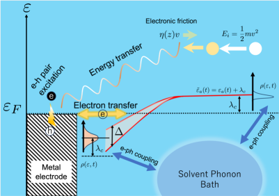
Figure 1: Schematic diagram of the time-dependent electron transfer and energy exchange in an electrochemical system.

We assume that the system is in equilibrium initially and the adsorbate is located sufficiently far away from the metal electrode so that any electron tunneling is impossible. The ions and atoms comprising the solvent are assumed to move infinitesimally in such a way that they can be represented by harmonic vibrations with infinite modes that form a phonon bath. At distances far from the surface of the electrode, the adsorbate orbital is characterized by a sharp resonance near the Fermi level ($\varepsilon_{F}$). As the adsorbate approaches the electrode, this state broadens as the energy level crosses $\varepsilon_{F}$ and becomes filled. The broadening is proportional to the square of the electronic overlap integrals between the metal and the adsorbate, represented by the resonance width $\Delta$. In addition, we assume that the adsorbate electron couples with the harmonic solvent modes linearly and shifts the energy level by an amount equivalent to the reorganization energy $\lambda$, a quantity proportional to the e-ph interaction. Furthermore, we assume that the adsorbate possesses a kinetic energy initially which is dissipated towards the excitation of e-h pairs in the metal electrode. These excitations consequently induce an electronic frictional force that slows down the adsorbate. There are of course other possible energy dissipation channels. However, in the present work, we are interested in non-adiabatic effects that are unique to a system involving a metal electrode.

In electrochemical systems, the electronic interaction between the metal and adsorbate is generally weak and only one spin state is typically occupied. Therefore, the electron repulsion interaction is neglected in the following. Further, to simplify our calculations, we invoke the so-called $trajectory~{}approximation$ which assumes that the motion of the adsorbate and the dynamics of the system are separated out. Simply put, the classical trajectory $R(t)$ of the adsorbate is known from the beginning. In most cases, this approximation works well for adsorbates with large masses or moving slowly. Therefore, our work treats the electrons and phonons quantum mechanically, while the adsorbate nuclear dynamics classically. This is justified when the thermal energy is larger than the frequency corresponding to the adsorbate nuclear motion (i.e., $k_{B}T>\hbar\omega_{a}$)Dou and Subotnik (2020), which we assume to be the case here.

The total Hamiltonian of the system described above may be represented by a time-dependent version of the Newns-Anderson-Schmickler modelSchmickler (1986) ($\hbar=1$),

$$H(t)= \varepsilon_{a}(t)n_{a}+\sum_{k}\varepsilon_{k}c_{k}^{\dagger}c_{k}+\sum_{k}\left[V_{ak}(t)a^{\dagger}c_{k}+H.c.\right]$$ (1)

$$+ \sum_{q}\omega_{q}b_{q}^{\dagger}b_{q}+(Z-n_{a})\sum_{q}\lambda_{q}\omega_{q}(b_{q}^{\dagger}+b_{q}),$$

where $n_{a}=a^{\dagger}a$. Here, $\varepsilon_{a}(t)=\varepsilon_{a}\left[R(t)\right]$ is the time-dependent energy level of the adsorbate whose Fock space is spanned by its electron annihilation and creation operators, $a$ and $a^{\dagger}$, respectively. $\varepsilon_{k}$ is the band energy of the non-interacting electrons with wavevector $k$ of the metal electrode filled up to the Fermi level, and $c_{k}(c_{k}^{\dagger})$ are their corresponding annihilation(creation) operators. $V_{ak}(t)=V_{ak}\left[R(t)\right]$ is the overlap integral between the metal $|k\rangle$ and moving adsorbate $|a\rangle$ electron states, whose time-dependence is assumed to be separable through $V_{ak}(t)=V_{ak}u(t)$Yoshimori and Makoshi (1986) where, $u(t)$ is some time-dependent function that will be specified later. $\omega_{q}$ is the frequency of the harmonic oscillators describing the solvent and $b_{q}(b_{q}^{\dagger})$ is the annihilation(creation) operator of the phonon of mode $q$. The harmonic displacements $b_{q}^{\dagger}+b_{q}$ couple linearly to the adsorbate electrons, $n_{a}$ with coupling strength, $\lambda_{q}$ and $Z$ is the charge of the oxidized adsorbate state.

We eliminate the e-ph coupling term in (1) by performing a nonperturbative canonical (Lang-Firsov) transformation $\tilde{H}=e^{S}He^{-S}$ where $S=\sum_{q}\lambda_{q}n_{a}(b_{q}^{\dagger}-b_{q})$. This results in the dressing of the adsorbate electron states as $\tilde{a}=ae^{-\lambda_{a}(b_{q}^{\dagger}-b_{q})}\equiv aX$, $\tilde{a}^{\dagger}=a^{\dagger}e^{\lambda_{q}(b_{q}^{\dagger}-b_{q})}\equiv a^{\dagger}X^{\dagger}$, and the shifting of the phonon operators $\tilde{b}_{q}=b_{q}-\lambda_{q}n_{a}$, $\tilde{b}^{\dagger}_{q}=b_{q}^{\dagger}-\lambda_{q}n_{a}$ due to the charging effect. The transformation leaves the metal electron states unchanged. The transformed Hamiltonian therefore reads

$$\tilde{H}(t)= \tilde{\varepsilon}_{a}(t)n_{a}+\sum_{k}\varepsilon_{k}c_{k}^{\dagger}c_{k}+\sum_{k}\left[\tilde{V}_{ak}(t)a^{\dagger}c_{k}+H.c.\right]$$ (2)

$$+ \sum_{q}\omega_{q}\left[b_{q}^{\dagger}b_{q}+Z\lambda_{q}(b_{q}^{\dagger}+b_{q})\right],$$

where $\tilde{\varepsilon}_{a}(t)=\varepsilon_{a}(t)+(2Z-1)\lambda$ is the adsorbate orbital energy level renormalized by e-ph coupling through the reorganization energy defined as $\lambda\equiv\sum_{q}\lambda_{q}^{2}\omega_{q}$; $\tilde{V}_{ak}(t)=V_{ak}(t)X^{\dagger}$ is the dressed electronic overlap integral. As in the local polaron problemHewson and Newns (1980), $V_{ak}$ is usually smaller than $\lambda_{q}$ and as a consequence, $\lambda$. It is therefore sufficient to replace $X^{\dagger}$ with its expectation valueChen et al. (2005) so that $\tilde{V}_{ak}(t)\approx V_{ak}(t)\langle X^{\dagger}\rangle=V_{ak}(t)\exp\left[\lambda_{q}^{2}(N_{q}+1/2)\right]$, where $N_{q}=\frac{1}{e^{\beta\omega_{q}}-1}$ corresponds to the phonon population and $\beta=1/k_{B}T$.

III Time-dependent electron transfer

III.1 Non-adiabatic adsorbate orbital occupancy

We are interested in the time-dependent adsorbate orbital occupancy which can be obtained from Keldysh Green’s functions through $\langle n_{a}(t)\rangle=\mathrm{Im}[G^{<}(t,t)]$. Our starting point is the nonequilibrium Dyson equation of the Keldysh lesser Green’s function

$$G^{<}(t,t^{\prime})=G_{0}^{<}(t,t^{\prime})+\int_{C}dt_{1}\int_{C}dt_{2}G_{0}^{<}(t,t_{1})\Sigma^{<}(t_{1},t_{2})G^{<}(t_{2},t^{\prime})$$ (3)

where $C$ is the time contour, $G^{<}_{0}$ is the unperturbed lesser Green’s function, and $\Sigma^{<}$ is the self-energy functional. To this end, the contour ordered Green’s function of the nonequilibrium system is expressed in a form that allows for a diagrammatic perturbation expansion by virtue of the Wick’s theorem. This is achieved by performing a series of transformations to arrive at an expression governed by the solvable, quadratic unperturbed Hamiltonian and a corresponding equilibrium density matrix. By setting the reference time $t_{0}\rightarrow-\infty$, and assuming that the initial interactions can be ignored, the contour $C$ can be identified as the Keldysh contourJauho et al. (1994) that begins and ends at $-\infty$. The contour integration in (3) is then converted to the real time integration by performing an analytical continuation using Langreth rulesLangreth (1976) resulting in

$$G^{<}=(1+G^{r}\Sigma^{r})G_{0}^{<}(1+G^{a}\Sigma^{a})+G^{r}\Sigma^{<}G^{a},$$ (4)

where $G^{r(a)}$ is the retarded(advanced) Green’s function, $\Sigma^{r(a)}$ is the retarded(advanced) self-energy, $\Sigma^{<}$ is the lesser self-energy and $G_{0}^{<}$ is the unperturbed lesser Green’s function. The first term is identically zeroOdashima and Lewenkopf (2017) within the wide-band approximation, which we shall heavily exploit in the following. In integral representation, $G^{<}$ may be written asJauho et al. (1994)

$$G^{<}(t,t^{\prime})=\int_{t_{0}}^{t}dt_{1}\int_{t_{0}}^{t}dt_{2}G^{r}(t,t_{1})\Sigma^{<}(t_{1},t_{2})G^{a}(t_{2},t^{\prime}).$$ (5)

The lesser self-energy appearing in (5) can be expressed in terms of the the renormalized electronic overlap integrals, $\Sigma^{<}(t_{1},t_{2})=\sum_{k}\tilde{V}_{ak}(t_{1})g^{<}_{k}(t_{1},t_{2})\tilde{V}^{*}_{ak}(t_{2})$ with $g^{<}_{k}(t_{1},t_{2})=if(\varepsilon_{k})\exp\left[-i\varepsilon_{k}(t_{1}-t_{2})\right]$ as the unperturbed Green’s function of the metal electrode electrons and $f(\varepsilon_{k})$ is their corresponding Fermi-Dirac distribution function. In the wide-band limit, the time-independent part of the electronic overlap integrals can be expressed in terms of the adsorbate level resonance width which we assume to be energy-independent through $\Delta=\pi|V_{ak}|^{2}\rho(\varepsilon_{k})$, with $\rho(\varepsilon_{k})$ is the density of states of the metal electrons. Changing the summation over $k$ to an integral over $\varepsilon$, the lesser self-energy takes the form

$$\Sigma^{<}(t_{1},t_{2})=i\int d\varepsilon f(\varepsilon)\sqrt{\frac{\Delta(t_{1})}{\pi}}\sqrt{\frac{\Delta(t_{2})}{\pi}}\ \exp\left[-i\varepsilon(t_{1}-t_{2})\right]$$ (6)

where, $\Delta(t)=\Delta u(t)^{2}$. Substituting (6) into (5) yields

$$G^{<}(t,t^{\prime})=i\int d\varepsilon f(\varepsilon)\int_{t_{0}}^{t}dt_{1}\sqrt{\frac{\Delta(t_{1})}{\pi}}\ \int_{t_{0}}^{t}dt_{2}\sqrt{\frac{\Delta(t_{2})}{\pi}}G^{r}(t,t_{1})\exp\left[-i\varepsilon(t_{1}-t_{2})\right]G^{a}(t_{2},t^{\prime}).$$ (7)

As in the polaron systems, we assume that the retarded Green’s function can be decoupled asZhu and Balatsky (2003)

$$G^{r(a)}(t,t^{\prime})= \mp i\theta(\pm t\mp t^{\prime})\langle\left\{\tilde{a}(t),\tilde{a}^{\dagger}(t^{\prime})\right\}\rangle_{el}\ \langle X(t)X^{\dagger}(t^{\prime})\rangle_{ph}$$ (8)

$$= ~{}\tilde{G}^{r(a)}(t,t^{\prime})\langle X(t)X^{\dagger}(t^{\prime})\rangle_{ph}.$$

Here, $X(t)=\exp\left[-\sum_{q}\lambda_{q}\left(b_{q}^{\dagger}e^{i\omega t}-b_{q}e^{-i\omega_{q}t}\right)\right]$, and $\langle\ldots\rangle_{e(ph)}$ is the expectation value with respect to electrons(phonons). The solvent correlation function $\langle X(t)X^{\dagger}(t^{\prime})\rangle_{ph}=\mathrm{Tr}\left[\rho_{ph}X(t)X^{\dagger}(t^{\prime})\right]\equiv B(t-t^{\prime})$ is given by

$$B(t)=\exp\left\{-\sum_{q}\lambda_{q}^{2}\ \left[(N_{q}+1)(1-e^{-i\omega_{q}t})+N_{q}(1-e^{i\omega t})\right]\right\}.$$ (9)

We assume that the solvent bath phonons are characterized by a spectral density $J(\omega)=\sum_{q=1}^{N}\lambda_{q}^{2}\omega_{q}^{2}\delta(\omega-\omega_{q})$. Replacing the $q$-mode summation with an integration over $\omega$ and noting the antisymmetric property of the spectral density, we rewrite (9) as

$$B(t)=\exp\left[\int_{-\infty}^{\infty}d\omega J(\omega)\ \frac{e^{i\omega t}}{e^{\beta\omega}-1}\right].$$ (10)

We choose the Drude-Lorentz form of the spectral density

$$J(\omega)=\frac{2\lambda}{\omega_{0}^{2}}\frac{\gamma\omega}{\gamma^{2}+\omega^{2}},$$ (11)

where $\omega_{0}$ is characteristic frequency of the solvent, and $\gamma$ is the cutoff frequency. $\lambda$ is typically in the range of $0.5-1.0$ eVSchmickler (1986). The $\omega$ integration can be performed analytically by contour integration giving

$$B(t)=\exp\left[\sum_{k=0}^{\infty}C_{k}e^{-\nu_{k}t}\right],$$ (12)

where $C_{k=0}=\frac{\lambda\gamma}{\omega_{0}^{2}}\left[\cot\left(\frac{\beta\gamma}{2}\right)-i\right]$, $C_{k\geq 1}=4\frac{\lambda\gamma}{\omega_{0}^{2}}\frac{\nu_{k}}{\beta\left(\nu_{k}^{2}-\gamma^{2}\right)}$, $\nu_{0}\equiv\gamma$, and $\nu_{k}=2\pi k/\beta$ is the $k$th Matsubara frequency. In the long time (adiabatic) limit, $B(t)\rightarrow 1$. The Matsubara-decomposed bath correlation function of the form (12) valid for a wide-range of temperature is frequently used in open quantum systemsTanimura and Kubo (1989); Tanimura (1990, 2020); Lambert et al. (2023). We next write the Dyson equation for $\tilde{G}^{r}$ as

$$\tilde{G}^{r}(t,t_{1})=G_{0}^{r}(t,t_{1})+\int d\tau\int d\tau^{\prime}G_{0}^{r}(t,\tau)\Sigma^{r}(\tau,\tau^{\prime})\tilde{G}^{r}(\tau^{\prime},t_{1})$$ (13)

where the retarded self-energy is defined as

$$\Sigma^{r}(\tau,\tau^{\prime})= \sum_{k}\bar{V}_{ak}(\tau)g_{k}^{r}(\tau,\tau^{\prime})\bar{V}^{*}_{ak}(\tau^{\prime})$$ (14)

$$= -i\int\frac{d\varepsilon}{\pi}\Delta u(\tau)u(\tau^{\prime})\exp\left[-i\varepsilon(\tau-\tau^{\prime})\right]\theta(\tau-\tau^{\prime})$$

$$= -i\Delta(\tau)\delta(\tau-\tau^{\prime}).$$

In the above expression, we used the wide band approximation and the definition of the unperturbed retarded Green’s function of the metal electrode $g_{k}^{r}(\tau,\tau^{\prime})=-i\theta(\tau-\tau^{\prime})\ \exp\left[-i\varepsilon_{k}(\tau-\tau^{\prime})\right]$ and $\bar{V}_{ak}$. With (14) the integral equation (13) can now be solvedLangreth and Nordlander (1991); Wingreen et al. (1989) yielding

$$\tilde{G}^{r}(t,t_{1})=-i\theta(t-t_{1})\exp\left\{-i\int_{t_{1}}^{t}d\tau\left[\tilde{\varepsilon}_{a}(\tau)-i\Delta(\tau)\right]\right\}.$$ (15)

The advanced Green’s function can also be obtained by following a similar procedure. Inserting (15) and (8) into (7), the time-dependent occupation number $\langle n_{a}(t)\rangle=\mathrm{Im}[G^{<}(t,t)]$ may be written as

$$\langle n_{a}(t)\rangle=\int d\varepsilon f(\varepsilon)\left|p(\varepsilon,t)\right|^{2},$$ (16)

where

$$p(\varepsilon,t)=\int_{t_{0}}^{t}dt^{\prime}\sqrt{\frac{\Delta(t^{\prime})}{\pi}}\ B(t^{\prime})\exp\left\{-i\int_{t^{\prime}}^{t}d\tau\left[\tilde{\varepsilon}_{a}(\tau)-i\Delta(\tau)-\varepsilon\right]\right\}.$$ (17)

The above expression can also be derived from the Heisenberg’s equations of motion approach as presented in Appendix A. We notice that $|p(\varepsilon,t)|^{2}$ may be interpreted as the time-dependent projected density of states (PDOS) of the adsorbate in electrochemical systems. The adiabatic expression of the occupation can be derived by ignoring the time dependence of $\Delta$ and $\tilde{\varepsilon}_{a}$. The exponential function may be replaced by $\exp\left\{-i\left[\tilde{\varepsilon}_{a}-i\Delta-\varepsilon\right](t-t^{\prime})\right\}$ and the analytical integration of (17) gives the adiabatic PDOS

$$|p(\varepsilon,t)|^{2}\rightarrow\rho^{ad}(\varepsilon)\equiv\frac{1}{\pi}\frac{\Delta}{\Delta^{2}+\left[\tilde{\varepsilon}_{a}-\varepsilon\right]^{2}},$$ (18)

which consequently yields the adiabatic orbital occupancy as

$$\langle n^{ad}_{a}\rangle=\int d\varepsilon f(\varepsilon)\rho^{ad}_{a}(\varepsilon).$$ (19)

In the following, we consider a classical scattering trajectory comprised of an incoming ($t<0$) and outgoing ($t>0$) regions. It is more physically meaningful to work in terms of the adsorbate position $R(t)$ rather than time. For simplicity, we neglect any motion parallel to the metal surface and assume that the adsorbate moves at a constant velocity $v$, such that the one-dimensional trajectory is given by $R(t)\approx z(t)=vt$. The details of numerical evaluation are presented in Appendix B wherein the PDOS is given in the $z$-representation as

$$\frac{1}{v^{2}}|p(\varepsilon,z)|^{2}=\int_{z_{0}}^{z}dz^{\prime}\sqrt{\frac{\Delta(z^{\prime})}{\pi}}\ B(z^{\prime})\exp\left\{-i\int_{z^{\prime}}^{z}dz^{\prime\prime}\left[\tilde{\varepsilon}_{a}(z^{\prime\prime})-i\Delta(z^{\prime\prime})-\varepsilon\right]\right\}.$$ (20)

We do not consider adsorption and assume that the adsorbate only scatters upon interacting with the metal surface. For convenience, we define the turning point (closest to the electrode) of the trajectory as $z\equiv 0.0$ Bohr. We note that this does not mean that the adsorbate is in contact with the surface of the electrode. In the present study, we consider a case in which the adsorbate is a proton ($Z=1$) with an initially empty orbital occupancy $\langle n_{a}(t_{0})\rangle=0$, and an energy level shifted above the Fermi energy ($\varepsilon_{F}$) by $\lambda$. We then parametrize $\Delta(z)$ and $\tilde{\varepsilon}_{a}(z)$ as Gaussian functions (see Figure 7)

$$\Delta(z) =\Delta\exp\left(-\alpha z^{2}\right)$$ (21)

$$\tilde{\varepsilon}_{a}(z) =(\varepsilon_{0}-\varepsilon_{\infty})\exp\left(-\kappa z^{2}\right)+\varepsilon_{\infty}+\lambda$$

where $\alpha=\kappa=0.015~{}\alpha_{0}^{-2}$ ($\alpha_{0}$ is the Bohr radius) is a parameter describing the decay of the electrode’s wavefunction into the solvent. $\Delta=0.01~{}$eV and $\varepsilon_{0}=-1.5~{}$eV are the values of the resonance width and adsorbate energy level at $z=0.0~{}$Bohr, and $\varepsilon_{\infty}=\varepsilon_{F}=0.0~{}$eV is the value of energy level when $z=\infty$. The parametrization of $\varepsilon(z)$ corresponds to a case in which an initially empty adsorbate orbital level crosses $\varepsilon_{F}$ and becomes occupied via the electron transfer from the metal surface. The opposite direction of electron transfer (from $\langle n_{a}(t_{0})\rangle=1$ to the metal surface) may also be investigated by changing the parameters in $\varepsilon(z)$, e.g., $\varepsilon_{0}=0.0~{}$ eV and $\varepsilon_{\infty}=-1.5~{}$ eV.

     

(a)

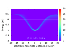
(b)

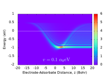
(c)

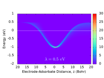
(d)

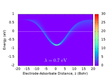
(e)

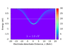
(f)

Figure 2: Time-dependent adsorbate projected density of states (PDOS) for different velocities (a)-(c) at $\lambda=0.5~{}$eV and reorganization energies (d)-(e) at $v=0.01~{}\alpha_{0}$eV as functions of energy and adsorbate-electrode distance. Other parameters are $\Delta=0.01$ eV, $\varepsilon_{0}=-1.5$ eV, $\varepsilon_{\infty}=\varepsilon_{F}=0.0$ eV, $\alpha=\kappa=0.015~{}\alpha_{0}^{-2}$, and $T=300$ K. The left- and right-hand sides of $z=0.0$ Bohr correspond to the incoming and outgoing parts of the trajectory, respectively.

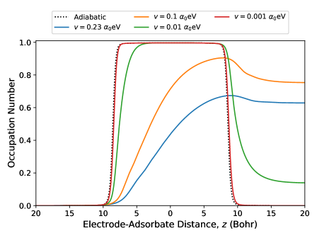
(a)

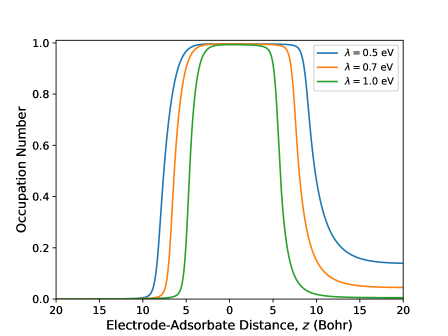
(b)

Figure 3: Adsorbate orbital occupancy at different (a) velocities when $\lambda=0.5$ eV and (b) reorganization energies when $v=0.01~{}\alpha_{0}$eV, using the parameters in Figure 2. The black dotted curves (a) correspond to the adiabatic orbital occupancy.

Figure 2 shows the plots of (20) obtained at $T=300$ K. The left- and right-hand sides of $z=0.0$ Bohr represent the incoming and outgoing portions of the trajectory, respectively. The upper panel shows the effects of velocity; (a) $v=0.001~{}\alpha_{0}$eV, (b) $v=0.01~{}\alpha_{0}$eV, and (c) $v=0.1~{}\alpha_{0}$eV when $\lambda=0.5$ eV. We note that the intensities are higher for smaller $v$, as suggested in (20). The intensity corresponds to the matching of the energy $\varepsilon$ with $\tilde{\varepsilon}_{a}(z)$ (see (20) or equivalently (63)), while the matching condition is relaxed because of $i\Delta$. The matching occurs once in the incoming and once in the outgoing portions in addition to the case when $z=0.0$ Bohr. For slowed adsorbate ($v=0.001~{}\alpha_{0}$eV), the PDOS intensities are mostly localized on a line given by $\varepsilon=\tilde{\varepsilon}_{a}(z)$. These become asymmetrically broadened as the adsorbate moves faster (Figure 2c). The asymmetry comes from the retardation of the function $p(\varepsilon,z)$ when $v$ is large. The lower panel shows the effects of the reorganization energy; (d) $\lambda=0.5$ eV, (e) $\lambda=0.7$ eV,and (f) $\lambda=1.0$ eV when $v=0.01~{}\alpha_{0}$eV. The shape of the peak intensities is generally similar to Figure 2b while the intensity is shifted upward by $\lambda$ as expected from the expression of $\tilde{\varepsilon}_{a}(z)$, which is the main effect of e-ph coupling. These findings corroborate the behavior of the adsorbate level occupations obtained by integrating the PDOS and the Fermi distribution functions over $\varepsilon$ and are shown in Figure 3.

Figure 3a shows the numerically calculated adsorbate orbital occupancy for different velocities when $\lambda=0.5$ eV. In the figure, $v=0.23~{}\alpha_{0}$eV correspond to the thermal velocity. The adiabatic occupation $\langle n_{a}^{ad}(z)\rangle$ (dotted lines) is highly symmetric in both incoming and outgoing portions of the trajectory with charge transfer occuring around $z\approx\pm 8.0$ Bohr. Near $z=0.0$ Bohr, $\langle n_{a}^{ad}(z)\rangle=1$ as expected since $\Delta$ is small. For non-zero $v$, the non-adiabatic effects manifest as significant deviations from $\langle n_{a}^{ad}(z)\rangle$ in both incoming and outgoing portions of the trajectory. This is especially prominent for adsorbate altitudes where $\tilde{\varepsilon}_{a}$ crosses $\varepsilon_{F}$. For faster speeds, the non-adiabatic occupations $\langle n_{a}(z)\rangle$ are strongly reduced and are extremely asymmetric, with orbital fillings starting to occur closer to $z=0.0$ Bohr in the incoming trajectory. When $v\geq 0.1~{}\alpha_{0}$eV, the orbital occupancies never reach 1 and are peaked at the outgoing portion. Furthermore, noticeable partial charge fillings persist long after the adsorbate has left the scattering region ($\tilde{\varepsilon}_{a}(z)\leq\varepsilon_{F}$). The reduction and asymmetry of $\langle n_{a}(z)\rangle$ can be easily deduced from the time-dependent PDOS with retardation effects as shown in Figure 2. Physically, these results highlight the inability of the electron system to return to its adiabatic ground state when the adsorbate is in motion; the breakdown of the Born-Oppenheimer approximation. The electronic system relaxation time $\tau\propto 1/\Delta$ becomes large when $\Delta$ is small. In electrochemical systems, $\Delta$ is typically small, on the order of a few meV implying a much longer $\tau$, and enhanced non-adiabaticity. Performing calculations with increased $\Delta$ when $v=0.1~{}\alpha_{0}$eV results in the reduction of asymmetric electron transfer. In vacuum where $\Delta$ is usually large, a slight asymmetry in $\langle n_{a}(z)\rangle$ is also evident and enhanced by increasing kinetic energy and metal work functionNakanishi et al. (1988). Further, additional non-adiabatic effects such as orbital overfillingsYoshimori and Makoshi (1986) are present. For much slower speeds, $\langle n_{a}(z)\rangle$ approaches the value of $\langle n_{a}^{ad}(z)\rangle$. When $v=0.001~{}\alpha_{0}$eV for example, the non-adiabatic effects are suppressed and the orbital occupancy very nearly coincides with the adiabatic value. This can also be seen in Figure 2a where PDOS retardations are vanishing and the peaks are highly localized. This confirms that our calculations reduce to the adiabatic value in the limit of vanishing velocity.

The effects of coupling with the solvent environment are shown in Figure 3b for adsorbate speed of $v=0.01~{}\alpha_{0}$eV. Within our chosen parameters, $\langle n_{a}(z)\rangle$ is visibly smaller and narrower when $\lambda=1.0$ eV, which can be traced back to the behavior of the renormalized adsorbate energy level depicted in Figure 7b in Appendix B and the time-dependent PDOS with retardation in Figure 2. At this adsorbate speed, several delocalized intensities are visible above $\varepsilon_{F}$ (Figure 2b). When $\lambda$ is increased, these are shifted upwards and do not contribute during $\varepsilon$ integration due to the energy range of $f(\varepsilon)$, resulting in narrower orbital occupancy. In contrast, for weaker $\lambda$, $\langle n_{a}(z)\rangle$ are broader due to the Fermi level crossings occuring farther away from $z=0.0$ Bohr. The persistent partial charge occupations in the outgoing portion are due to the minimal shifting (compared to strong $\lambda$) of the PDOS intensities which enables the retardation effects to contribute during $\varepsilon$ integrations. When $v=0.1~{}\alpha_{0}$eV, the non-adiabatic effects are amplified and the main effects of $\lambda$ is to reduce the occupation.

III.2 Non-adiabatic electron transfer rate

We obtain the distance-dependent electron transfer (reduction) rate by dividing the occupation with the electron system’s relaxation time $1/2\Delta$, giving $k(z)=2\Delta(z)\langle n_{a}(z)\rangle$. The total rate $k$ is the sum of $k(z)$ over the whole path of the adsorbate. Employing similar procedure derives the adiabatic rate $k_{ad}$ from (19). In Appendix C, we show that in the $k_{B}T\gg\Delta$ limit, $k_{ad}$ reduces to the electron transfer rate in the Marcus theory.

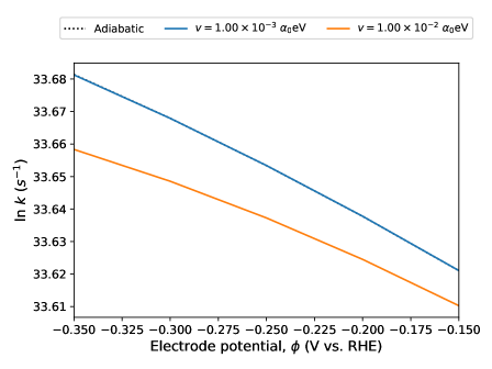
(a)

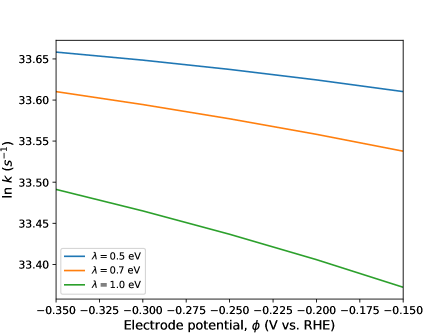
(b)

Figure 4: Electron transfer rate for different (a) velocities when $\lambda=0.5$ eV and (b) reorganization energy when $v=0.01~{}\alpha_{0}$eV as a function of electrode potential $\phi$ vs reversible hydrogen electrode (RHE) using the same parameters as in Figure 2. The black dotted line in (a) corresponds to the adiabatic rate.

Figure 4 shows the electron transfer rates for different $v$ and $\lambda$ as functions of the electrode potential $\phi$ vs. reversible hydrogen electrode (RHE). The range of $\phi$ is chosen to conform with the potential window of experimentally observed reduction rate of protonHamelin and Weaver (1987). The cathodic transfer coefficient $\alpha$ which is proportional to the Tafel slope is observed to decrease (increase) at increasingly (decreasingly) negative $\phi$. While we do not aim a quantitative comparison, to within our choice of parameters, we notice that the slopes of our computed $k$ and hence $\alpha$ in both most and least negative regions of $\phi$ are generally shown to exhibit the same tendencies as the experimental observation. Figure 4a shows that when the velocity is decreased, the electron transfer rate $k$ approaches the adiabatic result for relatively weak coupling with solvent modes ($\lambda=0.5$ eV). Similar conclusions can be drawn for other values of $\lambda$. We find that $v=0.001~{}\alpha_{0}$eV is slow enough to closely coincide with $k_{ad}$. At this adsorbate speed, the system can be considered as nearly adiabatic. In contrast, fast moving adsorbates significantly hinder the electron exchange resulting in the decrease of $k$. This is especially prominent when $v=0.23~{}\alpha_{0}$eV (not shown) where $k$ is about four times lesser compared to $k_{ad}$. The effects of coupling with the solvent modes shown in Figure 4b follow closely the results for $\langle n_{a}(z)\rangle$ at different strengths of $\lambda$, i.e., weak (strong) $\lambda$ results in higher (lower) electron transfer rates. The solvent effectively screens the tunneling electron and renormalizes the adsorbate energy level, resulting in the decrease of orbital occupancy and hence $k$.

IV Energy dissipation

A moving adsorbate needs to dissipate the kinetic energy to be adsorbed on the surface. Possible dissipation channels under an electrochemical condition are the excitation of vibration in solution and the creation of e-h pairs in metal electrode. Under our chosen parameters of the adsorbate velocity and temperature, the phonon correlation function $B(t)$ plays a minor role and thus we will concentrate on the latter channel. With the polaron transformed Hamiltonian (2), let us investigate the total amount of the energy dissipation by integrating the rate of change as derived in Appendix D

$$\dot{\mathcal{E}}=\langle\dot{\tilde{H}}\rangle=\dot{\tilde{\varepsilon}}_{a}(t)\langle n_{a}(t)\rangle\ +\frac{\dot{\Delta}(t)}{\sqrt{\pi\Delta(t)}}\int d\varepsilon f(\varepsilon)\Im[p(\varepsilon,t)],$$ (22)

where $p(\varepsilon,t)$ is given by (17). Note that (22) is the same as that derived for vacuum conditionMizielinski et al. (2005) with the exception of the renormalized adsorbate energy level and the presence of solvent correlation function in $p(\varepsilon,t)$. On the other hand, the amount of average energy transfered non-adiabatically $\bar{E}$ can be obtained by integrating the rate below which is derived following the substitution of $\langle n_{a}(t)\rangle$ with $\langle\delta n_{a}(t)\rangle=\langle n_{a}(t)\rangle-\langle n_{a}^{ad}(t)\rangle$ and $p(\varepsilon,t)$ with $\delta p(\varepsilon,t)=p(\varepsilon,t)-p^{ad}(\varepsilon,t)$

$$\dot{\bar{E}}=\dot{\tilde{\varepsilon}}_{a}(t)\langle\delta n_{a}(t)\rangle+\ \frac{\dot{\Delta}(t)}{\sqrt{\pi\Delta(t)}}\int d\varepsilon f(\varepsilon)\Im[\delta p(\varepsilon,t)].$$ (23)

Figure 5 shows the non-adiabatic average energy transfer rate computed for $v=0.01~{}\alpha_{0}$eV and different values of $\lambda$. For all strengths of $\lambda$ and in both incoming and outgoing parts of the trajectory, the rate is peaked at the positions where $\tilde{\varepsilon}_{a}(z)\simeq\varepsilon_{F}$. The peak position is closer to the turning point ($z=0.0$ Bohr) for stronger $\lambda$, in accordance with the position dependent parameters discussed in Appendix B. It was shownSchönhammer and Gunnarsson (1980) previously that the largest contribution to the average energy transfer $\bar{E}$ is proportional to $\sim 1/\Delta$.

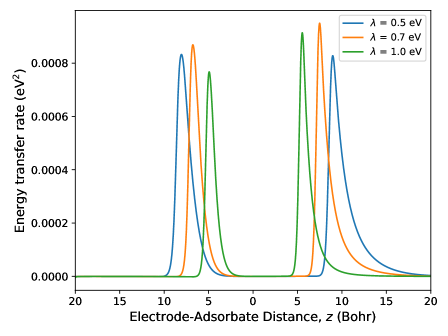
Figure 5: Average energy transfer rate of an adsorbate scattering on a metal electrode at speed of $v=0.01~{}\alpha_{0}$eV for different strengths of coupling with solvent modes $\lambda$. Other parameters are $\Delta=0.01$ eV, $\varepsilon_{0}=-1.5$ eV, $\varepsilon_{\infty}=\varepsilon_{F}=0.0$ eV, and $\alpha=\kappa=0.015~{}\alpha_{0}^{-2}$.

This implies that $\bar{E}$ is large when the Fermi level crossings occur at distances far from the metal surface, where $\Delta$ is small. In our case, $\bar{E}$ can be obtained by integrating (23) over the whole path which yields the following tendency: $\bar{E}(\lambda=0.5~{}\mathrm{eV})>\bar{E}(\lambda=0.7~{}\mathrm{eV})>\bar{E}(\lambda=1.0~{}\mathrm{eV})$. Clearly, from Figure 5, Fermi level crossing occurs farthest from the metal electrode when $\lambda=0.5~{}$eV, supporting the above average energy loss tendency. Within the trajectory approximation, the effects of velocity to the average energy exchange rate can be indirectly inferred from Figure 3 and the fact that $\dot{\bar{E}}$ is proportional to $\langle\delta n_{a}\rangle=\langle n_{a}\rangle-\langle n_{a}^{ad}\rangle$. When the adsorbate velocity is small, $\dot{\bar{E}}$ features nearly symmetric peaks centered at distances where Fermi level crossings occur. On the other hand, when the adsorbate moves faster, we notice peculiar energy gains ($\dot{\bar{E}}<0$) on the way out of the scattering region. This is mainly due to $\langle\delta n_{a}\rangle$ being negative within this range as can be deduced from the difference $\langle n_{a}\rangle-\langle n_{a}^{ad}\rangle$ in Figure 3.

IV.1 Electronic friction coefficient

The e-h excitations near the Fermi level of the electrode induced by the approaching adsorbate give rise to a frictional force that slows it down. The nuclear dynamics is essentially described by the Langevin equation ($m=1$)

$$\ddot{z}(t)=-\frac{dU(z)}{dz}-\int_{t_{0}}^{t}d\tau K(t-\tau)v(\tau)+\zeta(t),$$ (24)

where $U(z)$ is the adsorbate-electrode adiabatic potential energy surface, $K(t-\tau)$ is the dissipative nonlocal kernel that depends on the memory of the system and $\zeta(t)$ is the random force. The second term in (24) is the frictional force and is related to $\zeta(t)$ through the fluctuation-dissipation theorem. Since we are interested in the force induced by low energy excitations, we assume that the frictional force is purely electronic. In the limit of slowly moving adsorbate (small $v(t)$), the friction kernel becomes local (Markovian) i.e., $K(t-\tau)=\delta(t-\tau)\eta(t)$, where $\eta(z(t))$ is the electronic friction coefficient. We do not wish to evaluate the full dynamics of adsorbate using (24). Instead, our goal is to derive an expression for the local electronic friction coefficient in the slow motion or equivalently, in the nearly adiabatic limit. Evaluating the frictional force integral in Markovian limit gives

$$\int_{t_{0}}^{t}d\tau K(t-\tau)v(\tau)=\eta[z(t)]v(t)\equiv\frac{\dot{\bar{E}}^{SM}}{v(t)},$$ (25)

where,

$$\dot{\bar{E}}^{SM}=\dot{\tilde{\varepsilon}}_{a}(t)\langle\delta n_{a}^{SM}(t)\rangle+\ \frac{\dot{\Delta}(t)}{\sqrt{\pi\Delta(t)}}\int d\varepsilon f(\varepsilon)\Im[\delta p^{SM}(\varepsilon,t)].$$ (26)

is the average energy transfer rate in the slow motion (SM) limit. For a vanishingly small values of $v$, $t$ becomes sufficiently large such that $B(t)\sim 1$. Following Mizielinski et al. (2005), we proceed by performing Taylor expansions of the time-dependent quantities near their adiabatic values

$$\tilde{\varepsilon}_{a}(t^{\prime})\approx\tilde{\varepsilon}_{a}(t)+(t-t^{\prime})\dot{\tilde{\varepsilon}}_{a}(t)$$ (27)

$$\Delta(t^{\prime})\approx\Delta(t)+(t-t^{\prime})\dot{\Delta}(t),$$

and inserting them into (17) resulting in

$$p(\varepsilon,t)= \sqrt{\frac{\Delta(t)}{\pi}}\int_{-\infty}^{0}d\tau\ \left[1+i\frac{\dot{E}_{a}(t)}{2}\tau^{2}-\tau\frac{\dot{\Delta}(t)}{2\Delta(t)}\right]$$ (28)

$$\times \exp\left\{-i\left[E_{a}(t)-\varepsilon\right]\tau\right\}.$$

where $E_{a}(t)\equiv\tilde{\varepsilon}_{a}(t)-i\Delta(t)$. To arrive at (28), we expanded the term proportional to the exponential of the small quantity $\dot{E}_{a}(t)$ and changed the integration to $\tau=t-t^{\prime}$ with $t_{0}\rightarrow-\infty$. Performing the Gaussian integration of the first term is straightforward and yields the adiabatic expression for $p$ and hence recover $\langle n_{ad}\rangle$ in (19). The succeeding terms in (28) correspond to the non-adiabatic corrections due to the adsorbate motion in SM limit. The nearly adiabatic orbital occupancy then takes the form

$$\langle n_{a}(t)\rangle =\int d\varepsilon f(\varepsilon)|p^{ad}(\varepsilon,t)+\delta p^{SM}(\varepsilon,t)|^{2}$$ (29)

$$=\langle n_{a}^{ad}(t)\rangle+\langle\delta n_{a}^{SM}(t)\rangle,$$

where $\delta p^{SM}(\varepsilon,t)$ is given by the 2nd and 3rd terms of (28), and the non-adiabatic component of the occupancy $\langle\delta n_{a}^{SM}(t)\rangle$ in the SM limit may be expressed as

$$\langle\delta n_{a}^{SM}(t)\rangle=-\pi\int d\varepsilon\frac{df(\varepsilon)}{d\varepsilon}\ \left\{\frac{\dot{\Delta}(t)}{\Delta(t)}\left[\varepsilon-\tilde{\varepsilon}_{a}(t)\right]+\dot{\tilde{\varepsilon}}_{a}(t)\right\}\ \rho^{2}_{a}(\varepsilon,t),$$ (30)

from which we obtain the first term of (26). To this end, we discarded the negligible terms proportional to the products $\delta p^{*SM}(\varepsilon,t)\delta p^{SM}(\varepsilon,t)$. We then performed integration by parts, and ignored the neglible first term. Here, $\rho_{a}(\varepsilon,t)$ is the adsorbate PDOS. Following similar procedure described above, second term of (26) is given by

$$\frac{\dot{\Delta}(t)}{\sqrt{\pi\Delta(t)}}\int d\varepsilon f(\varepsilon)\Im[\delta p^{SM}(\varepsilon,t)] =\ -\pi\int d\varepsilon\frac{df(\varepsilon)}{d\varepsilon}\frac{\dot{\Delta}(t)}{\Delta(t)}\left[\varepsilon-\tilde{\varepsilon}_{a}(t)\right]$$ (31)

$$\times\left\{\frac{\dot{\Delta}(t)}{\Delta(t)}\left[\varepsilon-\tilde{\varepsilon}_{a}(t)\right]+\dot{\tilde{\varepsilon}}_{a}(t)\right\}\ \rho^{2}_{a}(\varepsilon,t).$$

Substituting (30) and (31) into (26) yields

$$\dot{\bar{E}}^{SM}=-\pi\int d\varepsilon\frac{df(\varepsilon)}{d\varepsilon}\ \left\{\frac{\dot{\Delta}(t)}{\Delta(t)}\left[\varepsilon-\tilde{\varepsilon}_{a}(t)\right]+\dot{\tilde{\varepsilon}}_{a}(t)\right\}^{2}\ \rho^{2}_{a}(\varepsilon,t).$$ (32)

This can be rewritten in terms of $z$ as

$$\dot{\bar{E}}^{SM}(z(t))=\eta(z)v^{2}.$$ (33)

where the coefficient of electronic friction is given by

$$\eta(z)=-\pi\int d\varepsilon\frac{df(\varepsilon)}{d\varepsilon}\ \left\{\frac{d\Delta(z)}{dz}\frac{\left[\varepsilon-\tilde{\varepsilon}_{a}(z)\right]}{\Delta(z)}+\frac{d\tilde{\varepsilon}_{a}(z)}{dz}\right\}^{2}\ \rho^{2}_{a}(\varepsilon,z).$$ (34)

Apart from the presence of the renormalized adsorbate energy level, our above result is equivalent to that of Mizielinski et al. (2005). Further, by setting $\Delta$ independent of $z$, (34) reduces to the expression of the electronic friction coefficient in vacuumDou and Subotnik (2018) where the adsorbate nuclear motion has been considered. At $T=0$, the derivative of the Fermi-Dirac distribution becomes a delta function, and the energy integration is trivial giving

$$\eta(z)=\pi\ \left\{\frac{d\Delta(z)}{dz}\frac{\left[\varepsilon_{F}-\tilde{\varepsilon}_{a}(z)\right]}{\Delta(z)}+\frac{d\tilde{\varepsilon}_{a}(z)}{dz}\right\}^{2}\ \rho^{2}_{a}(\varepsilon_{F},z).$$ (35)

Figure 6a shows $\eta(z)$ at $T=300$ K for different values of the reorganization energy. Since $v$ is assumed to be a constant, $\eta(z)$ essentially dictates the behavior of the average energy transfer in SM limit. The curves are highly symmetric in both portions of the trajectory and exhibit similar tendencies with the average energy transfer rate for non-negligible $v$ as seen in Figure 5. The peaks are centered at an adsorbate altitude where the adsorbate energy level crosses the Fermi level. This level crossing occurs closer to the electrode’s surface when $\lambda$ is strong, implying that $\dot{\bar{E}}^{SLM}(z(t))$ and hence the electronic frictional force is maximum when the coupling with solvent modes is minimum.

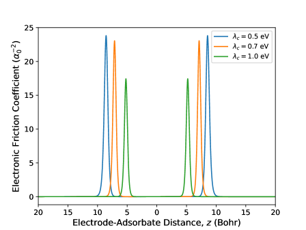
(a)

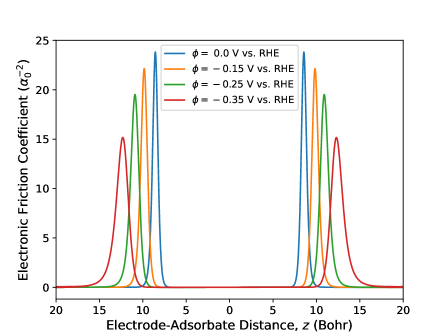
(b)

Figure 6: Electronic friction coefficient for different (a) $\lambda$ when electrode potential $\phi=0.0$ V and (b) $\phi$ when $\lambda=0.5$ eV as a function of $z$. Other parameters are the same as in Figure 5.

The effects of the electrode potential on the electronic friction coefficient when $\lambda=0.5$ eV is depicted in Figure 6b. Negative values of the electrode potential $\phi$ means shifting $\tilde{\varepsilon}_{a}(z)$ downward relative to $\varepsilon_{F}$, and then shifting the Fermi level crossings away from the metal electrode. When $\phi=-0.35$ V vs. RHE, for example, $\eta(z)$ is significantly broadened and lowered. This indicates that an increasing $\phi$ would make the frictional force act on a much wider range of $z$, thus increasing the average energy transfer. This leads to the important consequence that increasing $\phi$ promotes the energy loss of an adsorbate and increase the likelihood of trapping on the metal surface.

IV.2 Electron-hole excitation

It is suggestive to investigate how exactly the electron-hole excitations arise from the perspective of the electrons of the metal electrode using the Hamiltonian (1). Working again in the slow-motion limit, the approaching adsorbate is seen by the metal electrons as a slowly varying perturbationBrako and Newns (1981b, 1980), which results in instantaneous phase shifts at the Fermi level. This phase shift is related to the electronic friction and hence it is possible to derive (35), provided that the low energy excitations are in the neighborhood of $\varepsilon_{F}$. Borrowing the methods from surface science, the probability $P(\varepsilon)$ of a system being excited with an energy $\varepsilon$ after the perturbation is switched off at $t=\infty$ isSchönhammer and Gunnarsson (1980); Schönhammer (1981); Brako and Newns (1980, 1981b)

$$P(\varepsilon)=\frac{1}{2\pi}\int_{-\infty}^{\infty}dte^{i\varepsilon t}P(t)$$ (36)

where

$$P(t)=\langle\psi(\infty)|\exp\left\{-i\left[H(\infty)-E_{0}\right]t\right\}|\psi(\infty)\rangle.$$ (37)

The electrons are assumed to be in their ground state $|\psi(0)\rangle$ at $t=0$ with an energy $E_{0}=\langle\psi(0)|H_{0}|\psi(0)\rangle$ before the perturbation was switched on. The excited state $|\psi(\infty)\rangle$ is obtained by applying the time evolution operator $U(\infty,0)$ to $|\psi(0)\rangle$. Doing so in (37) and switching from Schrödinger to Heisenberg picture, with $H_{H}(\infty)=U(\infty,0)H(\infty)U(\infty,0)$, yields

$$P(t)=\langle\psi(0)|\exp\left[-iH_{H}(\infty)t\right]|\psi(0)\rangle e^{iE_{0}t}.$$ (38)

To obtain $H_{H}(\infty)$, we need the expressions for the electron operators $c_{k}^{\dagger}$ and $c_{k}$ in the Heisenberg picture. The procedure is rather lengthy, and we only summarize the important steps and results here. For more details, we refer the readers to the original paper of Brako and Newns in Reference Brako and Newns (1981a). To proceed, one begins by inserting expression (57) for annihilation operator $a$ that was derived using equations of motion into (50) to get $c_{k}$. The resulting expressions for $c_{k}$ is then simplified in the slow limit of the motion. Doing similarly for $c_{k}^{\dagger}$, the electronic Hamiltonian of the metal electrode may be written as

$$H_{H}(\infty)=\sum_{k}\varepsilon_{k}c_{k}^{\dagger}(\infty)c_{k}(\infty)=\frac{i}{2\pi\rho(\varepsilon_{k})}\ \sum_{k^{\prime},k^{\prime\prime}}\int dt\int ds\delta(t-s)\dot{F}_{k^{\prime},k^{\prime\prime}}(t,s)c^{\dagger}_{k^{\prime\prime}}c_{k^{\prime}},$$ (39)

where $\dot{F}_{k^{\prime},k^{\prime\prime}}(t,s)=\frac{\partial}{\partial t}\left\{e^{i\varepsilon_{k^{\prime\prime}}s}e^{-i\varepsilon_{k^{\prime}}t}e^{-2i\left[\delta(\varepsilon_{k^{\prime}},t)-\delta(\varepsilon_{k^{\prime\prime}},s)\right]}\right\}$, and $\delta(\varepsilon_{k},t)=\arctan\left[\frac{\Delta(t)}{\varepsilon_{k}-\tilde{\varepsilon}_{a}(t)}\right]$ is the phase shift. Integrating over $s$, (39) takes the form

$$H_{H}(\infty)=H_{0}+\sum_{k,k^{\prime}}U_{k,k^{\prime}}c_{k}^{\dagger}c_{k^{\prime}},$$ (40)

where $H_{0}=\sum_{k}\varepsilon_{k}c_{k}^{\dagger}c_{k}$ is the unperturbed Hamiltonian of the metal electrons and $U_{k,k^{\prime}}=\frac{1}{\pi\rho(\varepsilon_{k})}\int dt\dot{\delta}(\varepsilon_{k},t)\exp\left[i(\varepsilon_{k}-\varepsilon_{k^{\prime}})t\right]$ may be considered as an off-shell scattering matrix from state $k$ to $k^{\prime}$. The energy difference between the two states $\Omega=\varepsilon_{k^{\prime}}-\varepsilon_{k}$ is the e-h excitation energy. $\Omega$ is typically small on the order of the inverse of the time scale by which $\dot{\delta}$ varies. (40) provides two main ways to calculate $P(t)$: The first is through the linked cluster expansion as done by Brako and Newns in Brako and Newns (1981a), and the second is through Tomononaga bosonization as proposed by Schrönhammer and Gunnarsson Schönhammer and Gunnarsson (1980). Either method yields the same expression for $P(t)$ at finite temperature as

$$P(t)=\exp\left\{\frac{1}{\pi^{2}}\int_{0}^{\infty}d\Omega\Omega\ |\delta(\Omega)|^{2}\left[\coth\left(\frac{\beta\Omega}{2}\right)(\cos\Omega t-1)-i\sin\Omega t\right]\right\},$$ (41)

where $\delta(\Omega)=\int e^{i\Omega t}\dot{\delta}(\varepsilon_{F},t)$. This allows us to calculate $P(\varepsilon)$ through (36). The strength of the delta function of $P(\varepsilon)$ corresponds to the Debye-Waller factor that describes the probability of the system to remain in its ground state. Computing for the second moment of $P(\varepsilon)$ gives the average energy transfer

$$\bar{E}(t)=\frac{1}{\pi^{2}}\int d\Omega\Omega^{2}\ |\delta(\Omega)|^{2}=\frac{1}{\pi}\int_{-\infty}^{\infty}dt\dot{\delta}(\varepsilon_{F},t)^{2}.$$ (42)

This allows us to write the average energy transfer rate as

$$\dot{\bar{E}}(t)=\frac{1}{\pi}\dot{\delta}(\varepsilon_{F},t)^{2}=\pi\ \left\{\frac{\dot{\Delta}(t)}{\Delta(t)}\left[\varepsilon_{F}-\tilde{\varepsilon}_{a}(t)\right]+\dot{\tilde{\varepsilon}}_{a}(t)\right\}^{2}\ \rho^{2}_{a}(\varepsilon_{F},t),$$ (43)

which is nothing but energy transfer rate in SM limit (26) at $T=0$. From (43), the coefficient of electronic friction in (35) is straightforwardly obtained.

Without resorting to the full numerical evaluation of $P(\varepsilon)$, it is possible to make some remarks on the e-h excitations in the context of electrochemical system at least in the high temperature limit. To the leading order, we may introduce approximations as $\coth(\beta\Omega/2)\approx 2/\beta\Omega$, $\cos\Omega t-1\approx\Omega^{2}t^{2}/2$ and $\sin\Omega t\approx\Omega t$ when $\Omega$ is substantially small. Using these, (41) can be expressed as

$$P(t)\approx\exp\left(-\bar{E}k_{B}Tt-i\bar{E}t\right),$$ (44)

which after evaluating the time integrals in (36) yields a Gaussian form of $P(\varepsilon)$ as

$$P(\varepsilon)=\frac{1}{\sqrt{2\pi\bar{E}k_{B}T}}\exp\left[-\frac{(\varepsilon-\bar{E})^{2}}{4\bar{E}k_{B}T}\right],$$ (45)

which is peaked at the values of the average energy transfer rate $\bar{E}$. Based on our results for $\bar{E}$ in the previous section, $P(\varepsilon)$ will be most shifted towards the loss portion for small $\lambda$. Another interesting property that could also be derived from $P(\varepsilon)$ is the adsorbate sticking probability defined as

$$S(\varepsilon_{i})=\int_{\varepsilon_{i}}^{\infty}P(\varepsilon)d\varepsilon,$$ (46)

which describes the probability of an adsorbate with an initial energy $\varepsilon_{i}$ being captured during its interaction with the metal electrode. Roughly speaking, when the average energy loss is larger than $\varepsilon_{i}$, $S\rightarrow 1$, or the adsorbate is likely to be adsorbed. Evaluating (46), using (45) and (43) for $v=0.01\alpha_{0}$eV gives $S(\lambda=0.5~{}\mathrm{eV})>S(\lambda=0.7~{}\mathrm{eV})>S(\lambda=1.0~{}\mathrm{eV})$. This implies that strong $\lambda$ results in small energy loss and the adsorbate is less likely to be trapped. Conversely, weak $\lambda$ promotes energy loss and the probability of the adsorbate to stick on the metal surface. We may also infer the effects of electrode potential on the e-h excitation probability and the adsorbate sticking probability. For some values of $\lambda$, an increasingly negative $\phi$ would shift the peaks of $P(\varepsilon)$ towards the loss portion of the spectra. This indicates that the sticking probability of the adsorbate is promoted when $\phi$ is increased.

V Summary and Conclusions

We have studied the non-adiabatic effects due to the dynamic adsorbate interacting with the metal electrode in the presence of solvent using the time-dependent Newns-Anderson-Schmickler model Hamiltonian. The electron transfer rate is studied in terms of the time-dependent adsorbate occupation derived using the nonequilibrium Green’s function formalism and the trajectory approximation. Our numerical calculations show that the electron transfer rate is significantly reduced for nonzero adsorbate velocities and large electron-bath phonons couplings. It is also shown that the rate is strikingly peaked at distances where the adsorbate energy crosses the Fermi level of metal electrode. These crossings occur away from (close to) the metal surface for the small (large) solvent reorganization energy $\lambda$. This results in significant energy loss for weak $\lambda$. For small adsorbate velocities, we derived the analytic expression of the electronic friction coefficient $\eta(z)$. $\eta(z)$ is strongly peaked at a distance where Fermi level crossings occur. When the electrode potential is made more negative, the crossing occurs away from the metal surface leading to higher energy transfer rate and hence larger energy loss. We also discussed the probability $P(\varepsilon)$ of the electron system being excited, from which we derived the average energy transfer rate and the coefficient of electronic friction. In the high temperature limit, we discussed the sticking probability obtained from $P(\varepsilon)$. Since $P(\varepsilon)$ is peaked at the average energy loss value, we conclude that the sticking probability is high when $\lambda$ is small and the electrode potential is high.

VI Acknowlegments

This research is supported by the New Energy and Industrial Technology Development Organization (NEDO) project, MEXT as “Program for Promoting Researches on the Supercomputer Fugaku” (Fugaku battery & Fuel Cell Project) (Grant No. JPMXP1020200301, Project No.: hp220177, hp210173, hp200131), Digital Transformation Initiative for Green Energy Materials (DX-GEM) and JSPS Grants-in-Aid for Scientific Research (Young Scientists) No. 19K15397. Some calculations were done using the supercomputing facilities of the Institute for Solid State Physics, The University of Tokyo.

Appendix A Occupation Number from Equations of Motion Approach

We can recover the results of nonequilibrium Green’s function formalism using equations of motion approach (EOM). The Heisenberg EOM for an operator $\hat{O}$ is given by

$$\frac{d\hat{O}}{dt}=i[\tilde{H},\hat{O}]$$ (47)

where $\tilde{H}$ is the canonically transformed Hamiltonian. For brevity, we drop the hats on the operators. The EOM of the adsorbate electron annihilation operator is

$$i\frac{d\tilde{a}(t)}{dt}=\tilde{\varepsilon}_{a}(t)\tilde{a}(t)+\sum_{k}V_{ak}(t)c_{k}(t),$$ (48)

with $\tilde{V}_{ak}(t)a^{\dagger}(t)=V_{ak}(t)\tilde{a}^{\dagger}(t)$. We also require the EOM of metal electron’s annihilation operator,

$$i\frac{dc_{k}(t)}{dt}=\varepsilon_{k}c_{k}(t)+V_{ak}^{*}(t)\tilde{a}(t)$$ (49)

Integrating (49) to solve for $c_{k}$ gives

$$c_{k}(t)=\exp\left[-i\varepsilon_{k}(t-t_{0})\right]c_{k}(t_{0})-i\int_{t_{0}}^{t}dt^{\prime}\exp\left[-i\varepsilon_{k}(t-t^{\prime})\right]V_{ak}^{*}(t^{\prime})\tilde{a}(t^{\prime}),$$ (50)

where $t_{0}$ is an initial reference time. We substitute this into (48) to arrive at

$$i\frac{d\tilde{a}(t)}{dt}= \tilde{\varepsilon}_{a}(t)\tilde{a}(t)+\sum_{k}V_{ak}(t)\exp\left[-i\varepsilon_{k}(t-t_{0})\right]c_{k}(t_{0})$$ (51)

$$- i\sum_{k}\int_{t_{0}}^{t}dt^{\prime}\exp\left[-i\varepsilon_{k}(t-t^{\prime})\right]V_{ak}(t)V_{ak}^{*}(t^{\prime})\tilde{a}(t^{\prime}).$$

The last term in (51) can be evaluated with the aid of the wide band limit resulting to

$$-i\sum_{k}\int_{t_{0}}^{t}dt^{\prime}\exp\left[-i\varepsilon_{k}(t-t^{\prime})\right]V_{ak}(t)V_{ak}^{*}(t^{\prime})\tilde{a}(t^{\prime})=-i\Delta(t)\tilde{a}(t),$$ (52)

which then yields

$$i\frac{d\tilde{a}(t)}{dt}=\left[\tilde{\varepsilon}_{a}(t)-i\Delta(t)\right]\tilde{a}(t)+\sum_{k}V_{ak}(t)\exp\left[-i\varepsilon_{k}(t-t_{0})\right]c_{k}(t_{0})$$ (53)

This can be integrated to give

$$\tilde{a}(t)= \exp\left\{-i\int_{t_{0}}^{t}dt^{\prime}\left[\tilde{\varepsilon}_{a}(t^{\prime})-i\Delta(t^{\prime})\right]\right\}\tilde{a}(t_{0})\ +\int_{t_{0}}^{t}dt^{\prime}\exp\left\{-i\int_{t^{\prime}}^{t}d\tau\left[\tilde{\varepsilon}_{a}(\tau)-i\Delta(\tau)\right]\right\}$$ (54)

$$\times \sum_{k}V_{ak}(t^{\prime})\exp\left[-i\varepsilon_{k}(t^{\prime}-t_{0})\right]c_{k}(t_{0}).$$

Inserting $1=e^{-\lambda_{q}(b{\dagger}_{q}-b_{q})}e^{\lambda_{q}(b^{\dagger}_{q}-b_{q})}\ \equiv X(t)X^{\dagger}(t)$ into the second term of (54) yields

$$\tilde{a}(t)= \exp\left\{-i\int_{t_{0}}^{t}dt^{\prime}\left[\tilde{\varepsilon}_{a}(t^{\prime})-i\Delta(t^{\prime})\right]\right\}\tilde{a}(t_{0})\ +\int_{t_{0}}^{t}dt^{\prime}\exp\left\{-i\int_{t^{\prime}}^{t}d\tau\left[\tilde{\varepsilon}_{a}(\tau)-i\Delta(\tau)\right]\right\}$$ (55)

$$\times \sum_{k}\tilde{V}_{ak}(t^{\prime})X(t^{\prime})\exp\left[-i\varepsilon_{k}(t^{\prime}-t_{0})\right]c_{k}(t_{0}).$$

As in the Keldysh formalism, we take $\tilde{V}_{ak}(t^{\prime})\approx V_{ak}(t^{\prime})\langle X^{\dagger}(t^{\prime})\rangle\equiv\bar{V}_{ak}(t^{\prime})$ for $V_{ak}\ll\lambda$. At this point, we emphasize the difference between $\tilde{V}$ and $\bar{V}$. With this, $\tilde{a}(t)$ takes the form

$$\tilde{a}(t)= \exp\left\{-i\int_{t_{0}}^{t}dt^{\prime}\left[\tilde{\varepsilon}_{a}(t^{\prime})-i\Delta(t^{\prime})\right]\right\}\tilde{a}(t_{0})\ +\int_{t_{0}}^{t}dt^{\prime}\exp\left\{-i\int_{t^{\prime}}^{t}d\tau\left[\tilde{\varepsilon}_{a}(\tau)-i\Delta(\tau)\right]\right\}$$ (56)

$$\times \sum_{k}\bar{V}_{ak}(t^{\prime})X(t^{\prime})\exp\left[-i\varepsilon_{k}(t^{\prime}-t_{0})\right]c_{k}(t_{0}).$$

Multiplying both sides of (56) with $X^{\dagger}(t)$ and using the decoupling approximation in (8), the expectation values with respect to the bath phonons gives

$$a(t)= \exp\left\{-i\int_{t_{0}}^{t}dt^{\prime}\left[\tilde{\varepsilon}_{a}(t^{\prime})-i\Delta(t^{\prime})\right]\right\}a(t_{0})\ \langle X(t_{0})X^{\dagger}(t)\rangle$$ (57)

$$+ \int_{t_{0}}^{t}dt^{\prime}\exp\left\{-i\int_{t^{\prime}}^{t}d\tau\left[\tilde{\varepsilon}_{a}(\tau)-i\Delta(\tau)\right]\right\}$$

$$\times \sum_{k}\bar{V}_{ak}(t^{\prime})B(t^{\prime}-t)\exp\left[-i\varepsilon_{k}(t^{\prime}-t_{0})\right]c_{k}(t_{0}).$$

Consequently, the adsorbate electron’s creation operator is obtained as

$$a^{\dagger}(t)= \exp\left\{i\int_{t_{0}}^{t}dt^{\prime}\left[\tilde{\varepsilon}_{a}(t^{\prime})+i\Delta(t^{\prime})\right]\right\}a^{\dagger}(t_{0})\ \langle X^{\dagger}(t_{0})X(t)\rangle$$ (58)

$$+ \int_{t_{0}}^{t}dt^{\prime}\exp\left\{i\int_{t^{\prime}}^{t}d\tau\left[\tilde{\varepsilon}_{a}(\tau)+i\Delta(\tau)\right]\right\}$$

$$\times \sum_{k}\bar{V}_{ak}^{*}(t^{\prime})B(t-t^{\prime})\exp\left[i\varepsilon_{k}(t^{\prime}-t_{0})\right]c_{k}^{\dagger}(t_{0}).$$

Using (57) and (58), the occupation number of the adsorbate is obtained from the expectation values of the adsorbate electron operators

$$\langle n_{a}(t)\rangle=\langle a^{\dagger}(t)a(t)\rangle.$$ (59)

In evaluating (59), the terms proportional to $\langle a^{\dagger}(t_{0})c_{k}(t_{0})\rangle$ and $\langle c_{k}^{\dagger}(t_{0})a(t_{0})\rangle$ are equal to zero since the adsorbate and metal electrodes electrons are assumed to be decoupled at a distant past ($t_{0}\rightarrow-\infty$). After some algebraic manipulations and changing the summation over $k$ into an integration over $\varepsilon$, we recover (16) as,

$$\langle n_{a}(t)\rangle=\int d\varepsilon f(\varepsilon)\left|\int_{t_{0}}^{t}dt^{\prime}\sqrt{\frac{\Delta(t^{\prime})}{\pi}}\ B(t^{\prime})\exp\left\{-i\int_{t^{\prime}}^{t}d\tau\left[E_{a}(\tau)-\varepsilon\right]\right\}\right|^{2}.$$ (60)

where $f(\varepsilon_{k})=\langle c_{k}^{\dagger}(t_{0})c_{k}(t_{0})\rangle$ is Fermi-Dirac distribution of the metal electrons, and $E_{a}(t)\equiv\tilde{\varepsilon}_{a}(t)-i\Delta(t)$ . To this end, we neglected the product of the first terms of (58) and (57) which is a rapidly decaying transient.

Appendix B Numerical Evaluation

In the position representation, the occupation number can be written as

$$\langle n_{a}(z)\rangle=\frac{1}{v^{2}}\int d\varepsilon f(\varepsilon)\left|p(\varepsilon,z)\right|^{2}.$$ (61)

$p(\varepsilon,z)$ is defined as

$$p(\varepsilon,z)=\int_{z_{0}}^{z}dz^{\prime}\sqrt{\frac{\Delta(z^{\prime})}{\pi}}\ B(z^{\prime})\exp\left\{-\frac{i}{v}\int_{z^{\prime}}^{z}dz^{\prime\prime}\left[\tilde{\varepsilon}_{a}(z^{\prime\prime})-i\Delta(z^{\prime\prime})-\varepsilon\right]\right\},$$ (62)

where we replaced the time dependence in the bath correlation function with $z$. Since $B(t)$ is maximum when $t=0$ and approaches $1$ when $t\rightarrow\infty$, we shift $B(z)$ by $z+|z_{min}|$ with $z_{min}=-20$ Bohr being the starting point in the incoming portion of the trajectory to account for this behavior. We do not consider adsorption and assume that the parameters $\Delta(z)$ and $\tilde{\varepsilon}_{a}(z)$ can be expressed as Gaussian functions (see (21)).

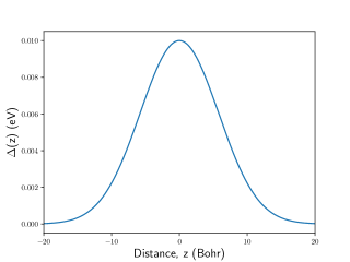
(a)

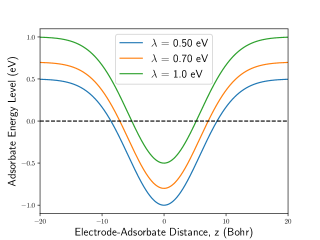
(b)

Figure 7: (a) The adorbate level resonance width $\Delta(z)$ for $\Delta=0.01~{}$eV and $\alpha=0.015~{}\alpha_{0}^{-2}$. (b) The adsorbate energy level $\tilde{\varepsilon}_{a}(z)$ for different strengths of reorganization energy $\lambda$. Other parameters are $\varepsilon_{F}=0.0~{}$eV, $\kappa=\alpha$, $\varepsilon_{0}=-1.5~{}$eV and $\varepsilon_{\infty}=\varepsilon_{F}$. The dashed black line corresponds to the electrode’s Fermi level.

Figure 7 shows the resonance width and the energy level of adsorbate as functions of $z$. Our chosen parameters correspond to a system consisting of an initially empty adsorbate orbital with an energy $\varepsilon_{\infty}$ that is shifted upwards by the reorganization energy due to e-ph coupling. As the adsorbate approaches near the electrode, the energy level starts to be filled when $\tilde{\varepsilon}_{a}(z)=\varepsilon_{F}$ and broadened by a magnitude $\Delta$ until $z=0.0$ Bohr where it is at maximum. As the adsorbate moves away from the electrode, this level gradually becomes unnocuppied again and returns to its value $\varepsilon_{\infty}$ as $z\rightarrow\infty$.

We numerically evaluate (61) by taking the derivative of (62) and integrating the resulting first-order complex differential equation,

$$\frac{dp(\varepsilon,z)}{dz}=\sqrt{\frac{\Delta(z)}{\pi}}B(z)-\frac{i}{v}\left[\tilde{\varepsilon}_{a}(z)-i\Delta(z)-\varepsilon\right]p(\varepsilon,z).$$ (63)

We assume that the electron transfer occurs at $T=300$ K and integrate (63) over the trajectory that starts at $z=-20~{}$Bohr and ends at $z=20~{}$Bohr with the interval $\Delta z=0.01~{}$Bohr using the complex ODE module of PYTHON. The initial condition corresponds to an empty adsorbate orbital at $z=-20$ Bohr. The energy integration is performed from $-10$ eV to $10$ eV with a grid size of $0.001$ eV. We consider different adsorbate velocities which includes $v=0.23~{}\alpha_{0}$eV, $v=0.1~{}\alpha_{0}$eV, $v=0.01~{}\alpha_{0}$eV, and $v=0.001~{}\alpha_{0}$eV. $v=0.23~{}\alpha_{0}$eV is the thermal velocity of an adsorbate with mass $m=1$ a kinetic energy equal to the thermal energy. In the absence of acceleration induced internally by the potential energy landscape of the adsorbate path and other external forces, this velocity may represent an upper limit in our study. The corresponding round trip simulation times $t=\frac{\hbar|z|}{v}$ for our chosen velocities are $114.5$ fs, $263.3$ fs, $2.633\times 10^{3}$ fs, and $2.633\times 10^{4}$ fs, respectively. As one may expect, the correlation function $B(t)$ requires a significant number of Matsubara frequencies $N_{k}\approx 10^{3}$ at low temperatures and can significantly slow down the calculations. However, when the electron transfer occurs at room temperature as is the case here, we found that it is sufficient to use $N_{k}=2$.

Appendix C Marcus Theory Limit

The electron transfer rate in the Marcus theory limit can be derived by first performing Fourier transform of the Lorentzian PDOS in (19) and writing the rate as

$$k=\frac{2\Delta}{\pi}\int d\varepsilon f(\varepsilon)\int_{-\infty}^{\infty}dte^{-\Delta|t|}e^{-i\left(\tilde{\varepsilon}_{a}-\varepsilon\right)t}.$$ (64)

Performing the thermal average as discussed inMohr and Schmickler (2000); Schmickler (1993) of (64) with respect to bath phonons results in

$$k=\frac{2\Delta}{\pi}\int d\varepsilon f(\varepsilon)\int_{-\infty}^{\infty}dte^{-\Delta|t|}e^{-i\left(\varepsilon_{a}+\lambda-\varepsilon\right)t}e^{-\frac{\lambda}{\beta}t^{2}}.$$ (65)

Marcus theory assumes that $k_{B}T\gg\Delta$ which is equivalent to neglecting $\Delta$ in the exponential in (65). Evaluating the time integral leads to the familiar Gaussian form of $k$ as

$$k=\frac{2\Delta}{\pi}\int d\varepsilon f(\varepsilon)\sqrt{\frac{\pi}{4\lambda k_{B}T}}\exp\left\{-\frac{\left[\varepsilon_{a}+\lambda-\varepsilon\right]^{2}}{4\lambda k_{B}T}\right\}.$$ (66)

Appendix D Derivation of Energy Exchange Rate

In order to arrive at (22), we first take the time derivative of (2) giving

$$\dot{\tilde{H}}=\dot{\tilde{\varepsilon}}_{a}(t)a^{\dagger}(t)a(t)+\sum_{k}\ \left[\dot{V}_{ak}(t)X^{\dagger}(t)a^{\dagger}(t)c_{k}(t)+h.c.\right].$$ (67)

To this end, the corresponding equations of motion for each operators have been used. After some algebraic manipulations, (67) may be expressed as

$$\dot{\tilde{H}}=\dot{\tilde{\varepsilon}}_{a}(t)a^{\dagger}(t)a(t)+\frac{\dot{\Delta}(t)}{2\Delta(t)}\sum_{k}\ \left[V_{ak}(t)X^{\dagger}(t)a^{\dagger}(t)c_{k}(t)+h.c.\right].$$ (68)

From the equations of motion of $a^{\dagger}$ and $c_{k}$,

$$a^{\dagger}(t)c_{k}(t)=\frac{1}{V_{ak}(t)X^{\dagger}(t)}\left[ia^{\dagger}(t)\dot{a}(t)-\tilde{\varepsilon}_{a}(t)a^{\dagger}(t)a(t)\right],$$ (69)

which yields

$$\dot{\tilde{H}}=\dot{\tilde{\varepsilon}}_{a}(t)a^{\dagger}(t)a(t)-\frac{\dot{\Delta}(t)}{\Delta(t)}\tilde{\varepsilon}_{a}(t)a^{\dagger}(t)a(t)\ +\frac{\dot{\Delta}(t)}{\Delta(t)}\Re\left[ia^{\dagger}(t)\dot{a}(t)\right].$$ (70)

Using (58) and the derivative of (57),

$$ia^{\dagger}(t)\dot{a}(t) =E_{a}(t)a^{\dagger}(t)a(t)+i\sum_{k}c_{k}^{\dagger}(t_{0})c_{k}(t_{0})|V_{ak}|^{2}\int_{t_{0}}^{t}dt^{\prime}u(t)u(t^{\prime})X(t)X^{\dagger}(t)$$ (71)

$$\times\exp\left\{i\left[\int_{t^{\prime}}^{t}E_{a}^{*}(t^{\prime\prime})dt^{\prime\prime}+\varepsilon_{k}(t^{\prime}-t)\right]\right\}+\ \exp\left[i\int_{t_{0}}^{t}E_{a}^{*}(t^{\prime})dt^{\prime}\right]a^{\dagger}(t_{0})c_{k}(t_{0}),$$

Substituting (71) into (70) and taking the expectation value, we obtain an expression for the energy transfer rate as

$$\dot{\mathcal{E}} \equiv\langle\dot{\tilde{H}}\rangle=\dot{\tilde{\varepsilon}}_{a}(t)\langle n_{a}(t)\rangle\ +\frac{\dot{\Delta}(t)}{\Delta(t)}\Re\left[i\int d\varepsilon f(\varepsilon)\sqrt{\frac{\Delta(t)}{\pi}}p^{*}(\varepsilon,t)\right],$$ (72)

$$=\dot{\tilde{\varepsilon}}_{a}(t)\langle n_{a}(t)\rangle\ +\frac{\dot{\Delta}(t)}{\sqrt{\pi\Delta(t)}}\int d\varepsilon f(\varepsilon)\Im\left[p(\varepsilon,t)\right]$$

with

$$p(\varepsilon,t)\equiv\int_{t_{0}}^{t}dt^{\prime}\sqrt{\frac{\Delta(t^{\prime})}{\pi}}B(t^{\prime})\exp\left\{i\int_{t^{\prime}}^{t}dt^{\prime\prime}\left[E_{a}(t^{\prime\prime})-\varepsilon\right]\right\}.$$ (73)

To this end, we note that the expectation value of the last term of (71) is zero for $t_{0}=-\infty$.

References

- Marcus (1965) R. A. Marcus, The Journal of Chemical Physics 43, 679 (1965).
- Hush (1958) N. S. Hush, The Journal of Chemical Physics 28, 962 (1958).
- Levich (1970) V. Levich, Physical Chemistry. An Advanced Treatise, edited by H. Eyring, D. Henderson, and W. Jost, Vol. Xb (Academic Press, 1970).
- Schmickler (1986) W. Schmickler, J. Electroanal. Chem 204, 31 (1986).
- Hewson and Newns (1974) A. C. Hewson and D. M. Newns, Japanese Journal of Applied Physics 13, 121 (1974).
- Citrin and Hamann (1977) P. H. Citrin and D. R. Hamann, Physical Review B 15, 2923 (1977).
- Song and Marcus (1993) X. Song and R. A. Marcus, The Journal of Chemical Physics 99, 7768 (1993).
- Sebastian (1989) K. L. Sebastian, The Journal of Chemical Physics 90, 5056 (1989).
- Smith and Hynes (1993) B. B. Smith and J. T. Hynes, The Journal of Chemical Physics 99, 6517 (1993).
- Mohr and Schmickler (2000) J.-H. Mohr and W. Schmickler, Physical Review Letters 84, 1051 (2000).
- Tanaka and Hsu (1999) S. Tanaka and C. P. Hsu, Journal of Chemical Physics 111, 11117 (1999).
- Wodtke et al. (2004) A. M. Wodtke, J. C. Tully, and D. J. Auerbach, International Reviews in Physical Chemistry 23, 513 (2004).
- Piechota and Meyer (2019) E. J. Piechota and G. J. Meyer, Journal of Chemical Education 96, 2450 (2019).
- Brako and Newns (1981a) R. Brako and D. M. Newns, Surface Science 108, 253 (1981a).
- Blandin et al. (1976) A. Blandin, A. Nourtier, and D. Hone, Journal de Physique 37, 369 (1976).
- Yoshimori et al. (1984) A. Yoshimori, H. Kawai, and K. Makoshi, Progress of Theoretical Physics Supplement 80, 203 (1984).
- Kasai and Okiji (1987) H. Kasai and A. Okiji, Surface Science 183, 147 (1987).
- Yoshimori and Makoshi (1986) A. Yoshimori and K. Makoshi, Progress in Surface Science 21, 251 (1986).
- Mizielinski et al. (2005) M. S. Mizielinski, D. M. Bird, M. Persson, and S. Holloway, Journal of Chemical Physics 122 (2005).
- Brako and Newns (1980) R. Brako and D. M. Newns, Solid State Communications 33, 713 (1980).
- Plihal and Langreth (2018) M. Plihal and D. C. Langreth, Journal of Chemical Physics 149 (2018).
- Newns (1986) D. M. Newns, Surface Science 171, 600 (1986).
- Kasai and Okiji (1991) H. Kasai and A. Okiji, Surface Science 242, 394 (1991).
- Gross and Brenig (1993) A. Gross and W. Brenig, Chemical Physics 177, 497 (1993).
- Lam et al. (2019) Y. C. Lam, A. V. Soudackov, and S. Hammes-Schiffer, Journal of Physical Chemistry Letters 10, 5312 (2019).
- Dou and Subotnik (2020) W. Dou and J. Subotnik, Journal of Physical Chemistry A 124, 757 (2020).
- Hewson and Newns (1980) A. C. Hewson and D. M. Newns, Journal of Physics C: Solid State Physics 13, 4477 (1980).
- Chen et al. (2005) Z. Z. Chen, R. Lü, and B. F. Zhu, Physical Review B - Condensed Matter and Materials Physics 71 (2005).
- Jauho et al. (1994) A.-P. Jauho, N. S. Wingreen, and Y. Meir, Physical Review B 50, 5528 (1994).
- Langreth (1976) D. Langreth, Linear and Non Linear Electron Transport in Solids, nato asi series b ed., edited by J. T. Devreese and E. van Doren, Vol. 17 (Plenum, 1976) p. 3.
- Odashima and Lewenkopf (2017) M. M. Odashima and C. H. Lewenkopf, Physical Review B 95 (2017).
- Zhu and Balatsky (2003) J. X. Zhu and A. V. Balatsky, Physical Review B 67 (2003).
- Tanimura and Kubo (1989) Y. Tanimura and R. Kubo, Journal of the Physical Society of Japan 58, 101 (1989).
- Tanimura (1990) Y. Tanimura, Physical Review A 41, 15 (1990).
- Tanimura (2020) Y. Tanimura, Journal of Chemical Physics 153 (2020).
- Lambert et al. (2023) N. Lambert, T. Raheja, S. Cross, P. Menczel, S. Ahmed, A. Pitchford, D. Burgarth, and F. Nori, Physical Review Research 5, 013181 (2023).
- Langreth and Nordlander (1991) D. C. Langreth and P. Nordlander, PHYSICAL REVIEW B 43, 2541 (1991).
- Wingreen et al. (1989) N. S. Wingreen, K. W. Jacobsen, and J. W. Wilkins, Physical Review B 40, 11834 (1989).
- Nakanishi et al. (1988) H. Nakanishi, H. Kasai, and A. Okiji, Surface Science 197, 515 (1988).
- Hamelin and Weaver (1987) A. Hamelin and M. J. Weaver, J. Electroanal. Chem. 223, 171 (1987).
- Schönhammer and Gunnarsson (1980) K. Schönhammer and O. Gunnarsson, Physical Review B 22, 1629 (1980).
- Dou and Subotnik (2018) W. Dou and J. E. Subotnik, Journal of Chemical Physics 148 (2018).
- Brako and Newns (1981b) R. Brako and D. M. Newns, J. Phys. C: Solid State Phys 14, 3065 (1981b).
- Schönhammer (1981) K. Schönhammer, Z. Phys. B-Condensed Matter 45, 23 (1981).
- Schmickler (1993) W. Schmickler, Surface Science 295, 43 (1993).