Group Sequential Design Under Non-proportional Hazards

Non-proportional hazards (NPH) are often observed in clinical trials with time-to-event endpoints. A common example is a long-term clinical trial with a delayed treatment effect in immunotherapy for cancer. When designing clinical trials with time-to-event endpoints, it is crucial to consider NPH scenarios to gain a complete understanding of design operating characteristics. In this paper, we focus on group sequential design for three NPH methods: the average hazard ratio, the weighted logrank test, and the MaxCombo combination test. For each of these approaches, we provide analytic forms of design characteristics that facilitate sample size calculation and bound derivation for group sequential designs. Examples are provided to illustrate the proposed methods. To facilitate statisticians in designing and comparing group sequential designs under NPH, we have implemented the group sequential design methodology in the gsDesign2 R package at https://cran.r-project.org/web/packages/gsDesign2/.
Keywords: group sequential design, non-proportional hazards, clinical trials, average hazard ratio, weighted logrank test, MaxCombo test.

1 Introduction

Non-proportional hazards (NPH) often arise in clinical trials involving time-to-event endpoints, such as oncology clinical trials with delayed treatment effects (Fig. 1 (a)) for immune-directed anticancer therapies; see, e.g., Reck et al., (2016) and Mok et al., (2019). In contrast to chemotherapy, immunotherapy activates the immune system to elicit an anti-tumor response, which can lead to delayed treatment effects (Mick and Chen,, 2015). Other examples of NPH include the cross-over pattern in survival curves (see Fig. 1 (b)) and the strong null scenario (see Fig. 1 (c)) (Wassie et al.,, 2023; Ramey et al.,, 2018).

(a) Delayed effect	(b) Cross-over	(c) Strong null

Figure 1: Three common cases of NPH.

When NPH are present, the commonly employed logrank test may exhibit reduced power compared to proportional hazards (PH). As a result, there is growing interest in exploring alternative approaches for quantifying treatment differences (León et al.,, 2020; Mukhopadhyay et al.,, 2020). In clinical trial development, the use of group sequential designs has become more prevalent, where the interim analyses (IA) enable multiple looks at the data before the study concludes. This facilitates early termination of the study when sufficient evidence is obtained. In this paper, we investigate three NPH methods within the framework of group sequential designs. Our focus is on deriving the analytical forms for design characteristics, including sample size, number of events, boundary calculation, and other operating characteristics.

To facilitate the development of the remainder of the paper, we begin with a brief introduction of group sequential designs containing $K\geq 2$ analyses with the test statistics of interest at the $k$-th analysis as $Z_{k}$. One of the key challenges in group sequential design is the selection of the upper bound $\{b_{k}\}_{k=1,\ldots,K}$ that can strongly control the overall Type I error, say $\alpha=0.05$. Using the alpha spending function approach (Demets and Lan,, 1994) to specify how much Type I error $\alpha_{k}$ spent on the $k$ -th analysis with $\sum_{k=1}^{K}\alpha_{k}=\alpha=0.05$, we can derive the upper boundaries $\{b_{k}\}_{k=1,\ldots,K}$ by sequentially solving

$$\alpha_{1}=Pr(\{Z_{k}\geq b_{k}|H_{0}),\;\;\;\alpha_{k}=Pr(\{Z_{k}\geq b_{k}\}\cap_{j=1}^{k-1}\{Z_{k}\leq b_{j}\}|H_{0})\forall\;2\geq k\geq K.$$

Given the upper bound $\{b_{k}\}_{k=1,\ldots,K}$, the overall type I error is the sum of probabilities of crossing any upper bound under the null hypothesis defined by

$$\text{type I error}=\sum_{k=1}^{K}Pr(\{Z_{k}\geq b_{k}\}\cap_{j=1}^{k-1}\{Z_{k}\leq b_{j}\}|H_{0}).$$

To calculate the above probability, we need to know the joint distribution of these test statistics $\{Z_{k}\}_{k=1,\ldots,K}$ under the null hypothesis. Similarly, we need to know the joint distribution of $\{Z_{k}\}_{k=1,\ldots,K}$ under the alternative hypothesis to calculate power by

$$\text{power}=\sum_{k=1}^{K}Pr(\{Z_{k}\geq b_{k}\}\cap_{j=1}^{k-1}\{Z_{k}\leq b_{j}\}|H_{1}).$$

Asymptotically, the sequence of test statistics $\{Z_{k}\}_{k=1,\ldots,K}$ is a normal process of independent increments (Scharfstein et al.,, 1997) in many commonly used test statistics for continuous, binary, and survival outcomes. The joint distribution of $\{Z_{k}\}_{k=1,\ldots,K}$ is multivariate normal with $E(Z_{k})=\theta\sqrt{\mathcal{I}_{k}}$ and $\text{Cov}(Z_{i},Z_{j})=\sqrt{\mathcal{I}_{i}/\mathcal{I}_{j}}$, $1\leq i\leq j\leq K$ with information level $\{\mathcal{I}_{k}\}_{k=1,\ldots,K}$ for the parameter $\theta$. This specific multivariate normal distribution is called the canonical joint distribution in Chapter 3 of Jennison and Turnbull, (2000). With the canonical joint distribution, the design characteristics can be derived in a unified approach analytically.

In this paper, we focus on group sequential design under three NPH methods, (M.1) the average hazard ratio test, (M.2) the weighted logrank test, and (M.3) the MaxCombo test. For the average hazard ratio test and weighted logrank test, the canonical joint distribution can be derived. However, the joint distribution is not multivariate normal for the MaxCombo test (Wang et al.,, 2021).

(M.1) Average hazard ratio (AHR) test. The hazard ratio (HR) is a widely used metric for assessing treatment effects in survival analysis. Under NPH, the natural extension to AHR has been recommended (Schemper et al.,, 2009; Kalbfleisch and Prentice,, 1981). Although various AHR methods have been suggested by Schemper et al., (2009), our focus is on the approach proposed by Mukhopadhyay et al., (2020) as it aligns with the widely used logrank test and Cox model estimation. We expand upon this approach by using a piecewise enrollment and proportional hazards model, and we also refine the asymptotic theory for group sequential design.

(M.2) Weighted logrank (WLR) test. In the context of NPH, researchers have investigated both the analysis and study design problems associated with the weighted log-rank test, which has the potential to improve power or reduce sample size (Fine,, 2007; Luo et al.,, 2019). To address the challenge of selecting time-dependent weights, different options have been proposed, including weight functions based on survival functions (Harrington and Fleming,, 1982) or at-risk proportions (Gehan,, 1965; Tarone and Ware,, 1977). In recent years, Magirr and Burman, (2019) and Magirr, (2021) have proposed a modestly weighted logrank test that avoids the issue of near-zero weighting for early observations, which can inflate Type I error.

(M.3) MaxCombo Test. Recent work in reviewing the WLR test has revealed that weight selection can be sensitive in different scenarios (Roychoudhury et al.,, 2021). To address this challenge, researchers have proposed a versatile MaxCombo test originally proposed by Lee, (1996). Lee, (2007) and Karrison, (2016) evaluated the performance of the MaxCombo test in various scenarios with small to moderate sample sizes and heavily censored data. The MaxCombo test mathematically selects the maximum value of a set of different WLR tests, each of which is designed to be powerful in detecting a specific NPH or PH pattern. As a result, the MaxCombo test can yield competitive and robust power, which is quite close to optimal across many scenarios, irrespective of whether it is PH or NPH.

In the existing NPH literature, researchers have investigated the aforementioned tests in trial designs, based on either simulation-based or analytical methodologies. However, there are certain limitations to existing work. For example, Yung and Liu, (2020) investigate the WLR test in fixed design. Their methodologies have not extended to group sequential designs. Wang et al., (2021) provide an analytical form for ground sequential design for the MaxCombo test, but do not cover the AHR test. Luo et al., (2019) discuss the logrank statistics and its variance-covariance structure under NPH, yet, many design operating characteristics (such as the boundaries and crossing probability) are not discussed. Roychoudhury et al., (2021) discuss the MaxCombo test to provide robust power based on simulations without an analytic form of design characteristic. Bautista and Anderson, (2021) analyze the sample size and power under multiple case studies, but the analytic forms are not presented.

The objective of this paper is to build on the existing literature to further enhance the aforementioned three tests. First, we thoroughly examine and present an analytical formulation for group sequential design utilizing the AHR test. Second, we derive analytical forms of group sequential design with a flexible choice of spending functions. Additionally, we establish both the efficacy and futility bounds in a canonical form for AHR and WLR tests, as well as the noncanonical form for the MaxCombo test. To facilitate statisticians in designing and comparing group sequential designs under NPH, we implement the group sequential design methodology in the gsDesign2 R package with multiple examples at https://merck.github.io/gsDesign2/. Finally, we establish the asymptotic equivalence between the AHR and WLR test statistics under a piecewise exponential model.

The remainder of this paper is organized as follows. In Section 2, we introduce the models of the three NPH methods. In Section 3, we present related design characteristics, including AHR, boundaries, crossing probabilities, sample size, and number of events. In Section 4, we present a simulation to verify the asymptotic theory proposed in Section 2. In Section 5, we apply the three approaches in a case study.

2 Test statistics

Without loss of generality, we focus on study designs involving two treatment groups with planned $n$ subjects and $K$ analyzes at times $t_{1},t_{2},\ldots,t_{K}$. Subjects are enrolled for a duration of $\tau_{a}$ and followed for an additional period of $\tau_{f}$, resulting in a total study duration of $\tau=\tau_{a}+\tau_{f}$. For the $i$-th subject ($i=1,\ldots,n$) at the $k$-th analysis, we use the following notation.

• $X_{i}$ denotes the treatment assignment for subject $i$: $X_{i}=0$ indicates the control arm and $X_{i}=1$ the treatment arm.

• $R_{i}$ denotes the time of study entry for subject $i$.

• $T_{i}$ denotes the time from study entry until an event occurs.

• $L_{i}$ denotes the time from study entry until a subject is lost to follow-up.

• $n_{k}=\sum_{i=1}^{n}I(R_{i}<\tau_{k})$ denotes the number of subjects included in analysis $k$.

• $U_{i,k}=\min(T_{i},L_{i},\tau_{k}-R_{i})$ denotes the observed survival time of subject $i$ at analysis $k$.

• $C_{i,k}=\min(L_{i},\tau_{k}-R_{i})$ denotes the observed censoring time of subject $i$ at analysis $k$.

• $\delta_{i,k}=I(U_{i}=T_{i,k})$ is the indicator that observation $i$ is censored for analysis $k$. If the $i$-th subject has an event at or prior to analysis time $\tau_{k}$, then $\delta_{i,k}=1$, otherwise $\delta_{i,k}=0$.

Based on the aforementioned notation, we suppose that Assumption 1 holds, which is common in survival analysis.

Assumption 1

Suppose within each treatment group, the following two conditions hold.

1. Survival times are independent and identically distributed with cumulative distribution function (cdf) $P(T_{i}\leq t)=F_{j}(t)$, probability density function (pdf) $f_{j}(t)=dF_{j}(t)/dt$, and hazard rate $\lambda_{j}(t)=f_{j}(t)/(1-F_{j}(t)).$

2. Loss-to-follow-up times $L_{i}$ are independent and identically distributed within each treatment group and are independent of $T_{i}$.

2.1 AHR

When the hazard ratio is not constant over time, AHR is a useful model with associated tools: AHR represents the average benefit over the period of observation (León et al.,, 2020). To calculate the AHR over time, a piecewise model will be used, as outlined in the assumption below.

Assumption 2

The AHR method assumes a piecewise model:

1. The enrollment rate is piecewise constant. Generally, it assumes that subjects enroll according to a Poisson process with an entry rate $g(u)>0$ for $u\geq 0$. Thus, the expected number of subjects enrolled by study time $t$ is simply $G(t)=\int_{0}^{t}g(u)du$. And in the AHR method, we assume that enrollment rates change at times $0=\tau_{e,0}<\tau_{e,1}<\ldots<\tau_{e,M_{e}}=\infty$ and $g(u)=\gamma_{m}\geq 0$ when $u\in(\tau_{e,m-1},\tau_{e,m}]$ for any $m=1,\ldots,M_{e}$.

2. The dropout rate is piecewise constant. We assume that the dropout rates change at times $0=\tau_{d,0}<\tau_{d,1}<\ldots<\tau_{d,M_{d}}=\infty$. And the dropout rate is equal to $\eta_{m}\geq 0$ in the interval of $(\tau_{d,m-1},\tau_{d,m}]$ for any $m=1,\ldots,M_{d}$.

3. The time-to-event rates are piecewise constants. We assume that the event rates can change at times $0=\tau_{f,0}<\tau_{f,1}<\ldots<\tau_{f,M_{f}}=\infty$ and the time-to-event rate equals $\lambda_{m}>0$ in the interval of $(\tau_{f,m-1},\tau_{f,m}]$ for any $m=1,\ldots,M_{f}$.

Based on the assumptions of the piecewise model described above, it is evident that there exist three sets of points at which changes occur, i.e., $\{\tau_{e,i}\}_{i=0,\ldots,M_{e}}$ for the enrollment rate, $\{\tau_{d,i}\}_{i=0,\ldots,M_{d}}$ for the dropout rates and $\{\tau_{f,i}\}_{i=0,\ldots,M_{f}}$ for the failure rates. These three sets of change points jointly divide the timeline with change points $\tau_{1},\ldots,\tau_{M}$:

$$\{\tau_{1},\ldots,\tau_{M}\}\triangleq\text{unique(}\{\{\tau_{e,i}\}_{i=0,\ldots,M_{e}}\cup\{\tau_{d,i}\}_{i=0,\ldots,M_{d}}\cup\{\tau_{f,i}\}_{i=0,\ldots,M_{f}}\}).$$

A visualization example of change points is shown in Figure 2. In this example, the enrollment rate has change points at the 2nd, 8th, 14th, and 20th months, and the failure rate has change points at the 4th month. Thus, they break the timeline into several intervals: $[0,2),[2,4),[4,8),[8,14),[14,20)$ and $[20,+\infty)$. Note that although the number of piecewise intervals is expected to be limited for simplicity and interpretability, it need not be if the hazard ratio and distributional properties over time are formed by more complex assumptions.

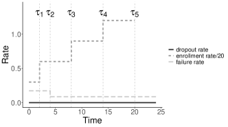
Figure 2: Piecewise enrollment/failure/dropout rate with vertical dash lines representing the change points cutoffs.

The three piecewise assumptions mentioned above provide a flexible approximation method for survival distributions that are commonly used. Furthermore, these assumptions are easy to explain to collaborators. The first assumption tailors the case where the enrollment rate is different in different periods. For example, the enrollment rate often accelerates early in the study until it reaches a steady state. The last two assumptions offer flexibility when dropout or failure rates change over time. This is motivated by time-varying outcome incidence. Different sets of change points for dropout rates and time-to-event rates have been found to be useful.

Note that the above piecewise assumption is an extension of Lachin and Foulkes, (1986): we extend their distribution of losses/survival from exponential to piecewise exponential. This extension offers more flexibility to fit cases in NPH, such as a delay in treatment effect in Section 1. Additionally, this extension is not trivial since the computation of design characteristics under piecewise exponential is more complicated than that exponential distribution.

When applying the AHR test in the time-to-event endpoint at the $k$-th analysis, we build the standardized treatment effect as the test statistics (Proschan et al.,, 2006):

$$Z_{k}^{(\text{ahr})}=\frac{\sum_{i=1}^{d_{k}}\Delta_{i}}{\sqrt{\text{Var}(\sum_{i=1}^{d_{k}}\Delta_{i}|H_{0})}},$$ (1)

where $d_{k}$ is the total number of events at analysis $k$. Here $\Delta_{i}=O_{i}-E_{i}$ with $O_{i}$ is the indicator that the $i$-th event occurred in the experimental arm, and $E_{i}=m_{i,1}/(m_{i,0}+m_{i,1})$ as the null expectation of $O_{i}$ given $m_{i,0}$ and $m_{i,1}$. The numbers $m_{i,0}$ and $m_{i,1}$ refer to the number of at-risk subjects prior to the $i$-th death in the control and experimental group, respectively. When conditioning on $m_{i,0}$ and $m_{i,1}$, $O_{i}$ has a Bernoulli distribution with parameter $E_{i}$. Thus, the null conditional mean and variance of $\Delta_{i}$ are 0 and $V_{i}=E_{i}(1-E_{i})$, respectively. Unconditionally, $\Delta_{i}$ are mean 0 random variables with variance $E(V_{i})$ under the null hypothesis. So, conditioned on $d_{k}$, we have $\text{Var}(\sum_{i=1}^{d_{k}}\Delta_{i}|H_{0}))=E(\sum_{i=1}^{d_{k}}V_{i}$).

As depicted in Section 2.1.3 of Proschan et al., (2006), the formulation of the stochastic process presented in Harrington et al., (1984) and Tsiatis, (1982) provides insight that the sequence of B values, denoted as ${B_{1},\ldots,B_{K}}$ with $B_{k}=\sqrt{t_{k}}Z_{k}^{\text{(ahr)}}$, follows a multivariate normal distribution that behaves asymptotically like a Brownian motion. Here $t_{k}$ is the information fraction at the $k$th analysis, that is,

$$t_{k}=\frac{\text{Var}(\sum_{i=1}^{d_{k}}\Delta_{i}|H_{0})}{\text{Var}(\sum_{i=1}^{d_{K}}\Delta_{i}|H_{0})}\approx\frac{d_{k}/4}{d_{K}/4}=d_{k}/d_{K},$$

by approximating $E(V_{i})=E(E_{i}(1-E_{i}))\approx 0.5(1-0.5)=1/4$ under the null hypothesis. Consequently, we show $Z_{k}^{\text{(ahr)}}$ has the canonical joint distribution with the following properties:

• $Z_{1}^{\text{(ahr)}},Z_{2}^{\text{(ahr)}},\ldots,Z_{K}^{\text{(ahr)}}$ have a multivariate normal distribution.

• $E(Z_{k}^{\text{(ahr)}})=0$ under the null hypothesis.

• $\text{Cov}(Z_{i}^{\text{(ahr)}},Z_{j}^{\text{(ahr)}})=\sqrt{t_{i}/t_{j}}$ for any $1\leq i\leq j\leq K$ under the null hypothesis.

Under the alternative hypothesis, if we denote the treatment effect as $\theta_{k}$ and rewrite $\mathcal{I}_{k,H_{0}}=1/\text{Var}(\sum_{i=1}^{d_{k}}\Delta_{i}|H_{0})$ in (1), then we have the asymptotic mean and variance of $Z_{k}^{\text{(ahr)}}$ as $\theta_{k}\sqrt{\mathcal{I}_{k,H_{0}}}$ and $\mathcal{I}_{k,H_{1}}/\mathcal{I}_{k,H_{0}}$, respectively. And the covariance is $\text{Cov}(Z_{i}^{\text{(ahr)}},Z_{j}^{\text{(ahr)}})=\frac{1}{\sqrt{t_{i}t_{j}}}\text{Cov}(B_{i},B_{j})=\frac{1}{\sqrt{t_{i}t_{j}}}\text{Var}(B_{i})=\sqrt{\frac{t_{i}}{t_{j}}}\frac{\mathcal{I}_{i,H_{0}}}{\mathcal{I}_{i,H_{1}}}$ under the alternative hypothesis. When the local alternative assumption is satisfied (see Appendix A.6), we have $\text{Cov}(Z_{i}^{\text{(ahr)}},Z_{j}^{\text{(ahr)}})\approx\sqrt{\frac{t_{i}}{t_{j}}}$, which is in the format of the canonical joint distribution introduced in Section 1.

2.2 WLR

The purpose of the WLR test is to compare the survival curves of two groups. In this scenario, the null hypothesis is stated as $H_{0}:\overline{F}_{0}(\cdot)=\overline{F}_{1}(\cdot)$, where $\overline{F}_{j}(\cdot)$ represents the complement of the cumulative distribution function (cdf) of the survival distribution for group $j\in\{0,1\}$.

Assumption 3

The WLR method is based on certain assumptions, which are outlined below.

1. the time of study entry $\{R_{i}\}_{i=1,\ldots,n}$ has continuous cdf denoted as $H(\cdot)$;

2. the time to loss of follow-up in group $j$, i.e., $\{L_{i}|X_{i}=j\}_{i\in\{X_{i}=j\}}$ has continuous cdf $G_{j}(\cdot)$.

Under the aforementioned assumptions, the WLR method employs the weighted logrank test, which is an extension of the logrank test that incorporates weights to examine the null hypothesis $H_{0}$. The test statistics for the $k$-th analysis are as follows:

$$Z_{k}^{(\text{wlr})}=\frac{U_{k}}{\sqrt{V_{k}}}=\frac{\sum\limits_{\{s:\;s<t_{k}\}}a(s)\left(X_{(s)}-\frac{\overline{Y}_{1}(s)}{\overline{Y}_{0}(s)+\overline{Y}_{1}(s)}\right)}{\sqrt{\sum\limits_{\{s:\;s<t_{k}\}}a(s)^{2}\frac{\overline{Y}_{0}(s)\overline{Y}_{1}(s)}{\left[\overline{Y}_{0}(s)+\overline{Y}_{1}(s)\right]^{2}}}}.$$ (2)

Here ${\{s:\;s<t_{k}\}}$ is the complete set of event times before the $k$-th analysis. The $X_{(s)}$ is the assigned treatment for the subject who fails at time $s$, and the $\overline{Y}_{j}(s)$ is the number of at-risk subjects in group $j$ at time $s$.

The numerator $U_{k}$ in (2) might not correspond to a measure of treatment efficacy. However, with some linear transformation, we can show $U_{k}$ as a weighted summation of the difference in estimated hazards in discrete time:

$$U_{k}=\sum\limits_{\{s:\;s<t_{k}\}}a(s)\frac{\overline{Y}_{0}(s)\overline{Y}_{1}(s)}{\overline{Y}_{0}(s)+\overline{Y}_{1}(s)}\left(\frac{X_{(s)}}{\overline{Y}_{1}(s)}-\frac{1-X_{(s)}}{\overline{Y}_{0}(s)}\right).$$

Following Appendix A.3 in Yung and Liu, (2020), one has

$$\sqrt{n_{k}}\left(U_{k}/n_{k}-\Delta_{k}\right)\overset{d}{\to}N(0,\widetilde{\sigma}^{2}_{b,k}),$$ (3)

where $\widetilde{\sigma}^{2}_{b,k}$ is a constant, $n_{k}$ is the sample size at the $k$-th look, and

$$\Delta_{k}=\int_{0}^{t_{k}}w(s)\frac{p_{0,k}\pi_{0,k}(s)\;p_{1,k}\pi_{1,k}(s)}{\pi_{k}(s)}\left[\lambda_{1}(s)-\lambda_{0}(s)\right]ds.$$ (4)

Here the term $p_{j,k}$ is the randomization probability of group $j$ at $k$-th analysis, i.e., $p_{j,k}=n_{j,k}/(n_{0,k}+n_{1,k})$. In addition, $\pi_{j,k}(t)$ is the expected at-risk probability of group $j$, i.e., $\pi_{j}(t)\triangleq E\left[\mathbbm{1}\{U_{i}\geq t\}|X_{i}=j\right]=\overline{F}_{j}(t)\overline{G}_{j}(t)H(\min\{\tau_{a},\tau-t\}).$ And $\pi_{k}(t)=p_{0,k}\pi_{0,k}(t)+p_{1,k}\pi_{1,k}(t)$ is the overall at-risk probability. The function $w(t)=\lim_{n\to\infty}a(t)$ denotes the limit of $a(t)$, which weights the different hazard ratios over time. In the literature, one of the popular weight functions is the Fleming-Harrington (FH) test

$$w(t)=\left[\bar{F}(t-)\right]^{p}\left[1-\bar{F}(t-)\right]^{q}$$

where $p\geq 0,q\geq 0$ and $\bar{F}(t-)$ is the left-continuous version of the Kaplan-Meier estimator for the pooled sample (see Section 2.1.6 in Karadeniz et al., (2017) and Section 2 in León et al., (2020)). In Figure 3, we visualize FH weights under 4 sets of $(p,q)$, that is, $(0,0),(0,0.5),(0.5,0)$ and $(0.5,0.5)$. From this figure, we find that when $p=q=0$, the WLR is reduced to the regular logrank test. Consequently, $Z_{k}^{(\text{wlr})}$ in (2) is reduced to the ordinary, unweighted logrank statistics. When $p=0$ and $q=0.5$, more weight is assigned to the later phase of the study. When $p=0.5$ and $q=0$, more weight is assigned to the early phase of the study.

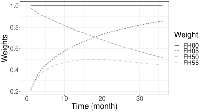
Figure 3: Visualization of different Fleming-Harrington weights (FH$xy$ represent $p=x/10,q=y/10$)

From Yung and Liu, (2020) the denominator in (2), $V_{k}$ has

$$V_{k}/n_{k}\overset{p}{\to}\sigma_{k}^{2}.$$ (5)

Here, the values of $\sigma_{k}$ vary depending on whether it is under the null hypothesis or the alternative hypothesis:

$$\left\{\begin{array}[]{ccl}\sigma_{k}^{2}|H_{1}&=&\int_{0}^{t_{k}}w(s)^{2}\frac{p_{0,k}\pi_{0,k}(s)\;p_{1,k}\pi_{1,k}(s)}{\left[p_{0,k}\pi_{0,k}(s)+p_{1,k}\pi_{1,k}(s)\right]^{2}}dv(s)\\ \sigma_{k}^{2}|H_{0}&=&\int_{0}^{t_{k}}w(s)^{2}\frac{p_{0,k}\pi_{0,k}(s)\;p_{0,k}\pi_{0,k}(s)}{\left[p_{0,k}\pi_{0,k}(s)+p_{0,k}\pi_{0,k}(s)\right]^{2}}dv(s)=\int_{0}^{t_{k}}w(s)^{2}\;\frac{p_{0,k}\pi_{0,k}(s)}{2}dv(s)\end{array}\right.,$$

where $v(t)=p_{0}v_{0}(t)+p_{1}v_{1}(t)$ is the failure probability with $v_{j}(t)$ representing the probability that a subject in group $j$ will experience an event within time $t$, i.e., $v_{j}(t)\triangleq E\left[\mathbbm{1}\{U_{i}\leq t,\delta_{i}=1\}|X_{i}=j\right]=\int_{0}^{t}f_{j}(s)\overline{G}_{j}(s)H(\min\{\tau_{a},\tau-s\})ds.$

Combining the results from (3) and (5), we show $Z_{k}^{\text{(wlr)}}$ has the canonical joint distribution (Wang et al.,, 2021):

• $Z_{1}^{\text{(wlr)}},Z_{2}^{\text{(wlr)}},\ldots,Z_{K}^{\text{(wlr)}}$ have a multivariate normal distribution.

• $E(Z_{k}^{\text{(wlr)}})=0$ under the null hypothesis.

• $\text{Cov}(Z_{i}^{\text{(wlr)}},Z_{j}^{\text{(wlr)}})=\sqrt{\sigma_{i}/\sigma_{j}}$ for any $1\leq i\leq j\leq K$ under the null hypothesis.

Under the alternative hypothesis, we have $E(Z_{k}^{\text{(wlr)}})=\sqrt{n_{k}}\Delta_{k}/\sigma_{k}$. When the local alternative assumption holds (see Appendix A.6 for detailed discussion), one can get the asymptotic variance of $Z_{k}^{(\text{wlr})}$ as 1 under both the null and alternative hypotheses.

2.3 MaxCombo

The MaxCombo test, proposed by Lee, (1996), considers the maximum value obtained from a combination of different WLR tests, enabling robust test sensitivity under a variety of scenarios:

$$Z_{k}^{(\text{mc})}=\max\left\{Z_{k}^{(\text{wlr}_{1})},Z_{k}^{(\text{wlr}_{2})},\ldots,Z_{k}^{(\text{wlr}_{L})}\right\},$$ (6)

where $Z_{k}^{(\text{wlr}_{i})}$ is a test statistic from a weighted logrank test.

Considering $Z_{k}^{(\text{mc})}$ involves a maximum operator, there is no canonical joint multivariate normal distribution. However, the asymptotic normal distribution of $Z_{k}^{(\text{wlr}_{i})}$ can be used to derive the type I error, power, and other design characteristics. In the following example, we demonstrate the calculation of the crossing probabilities in the MaxCombo test using the WLR test.

Example 1

In a group sequential design with 2 analyses, the upper and lower bound at the interim analysis are $a_{1}$ and $b_{1}$ and the upper bound at the final analysis is $b_{2}$. A MaxCombo test is applied with 2 WLR tests. The probability of crossing an upper bound only at the final analysis is

$$\text{Pr}(a_{1}<Z_{1}^{(\text{mc})}<b_{1},Z_{2}^{(\text{mc})}>b_{2}).$$

The above probability can be written as

$$\underbrace{\text{Pr}(Z_{1}^{(\text{mc})}<b_{1})}_{\mathcal{A}_{1}}-\underbrace{\text{Pr}(Z_{1}^{(\text{mc})}<a_{1})}_{\mathcal{A}_{2}}-\underbrace{\text{Pr}(Z_{1}^{(\text{mc})}<b_{1},Z_{2}^{(\text{mc})}<b_{2})}_{\mathcal{A}_{3}}+\underbrace{\text{Pr}(Z_{1}^{(\text{mc})}<a_{1},Z_{2}^{(\text{mc})}<b_{2})}_{\mathcal{A}_{4}}.$$

The first term $\mathcal{A}_{1}$, can be re-written as

$$\mathcal{A}_{1}=\text{Pr}(Z_{1}^{(\text{wlr}_{1})}<b_{1},Z_{1}^{(\text{wlr}_{2})}<b_{1}),$$

which can be solved by the asymptotic distribution of $\left(Z_{1}^{(\text{wlr}_{1})},Z_{1}^{(\text{wlr}_{2})}\right).$ Similar logic applies in the second term $\mathcal{A}_{2},\mathcal{A}_{3}$, and $\mathcal{A}_{4}$.

Based on the example provided above, we observe that the crucial aspect lies in determining the asymptotic distribution of the set $\{Z_{k}^{(\text{wlr}_{i})}\}_{k=1,\ldots,K;\;i=1,\ldots,L}$. However, this task is challenging due to the covariance matrix encompassing three distinct types of correlations, making it a nontrivial endeavor. Without loss of generality, we take the WLR test with FH weighting as an illustration example to show the correlation structure.

The first type of correlation is the correlation within the analysis between different tests. In the context of a fixed analysis $k$, the correlation between two WLR tests with FH weights of FH$(p_{i},q_{i})$ and FH$(p_{j},q_{j})$ is represented as

$$\text{Corr}\left(Z_{k}^{(\text{wlr}_{i})},Z_{k}^{(\text{wlr}_{j})}\right)=\text{Var}\left(U_{k}^{(\text{wlr}_{ij})}\right)\bigg{/}\sqrt{\text{Var}\left(U_{k}^{(\text{wlr}_{i})}\right)\text{Var}\left(U_{k}^{(\text{wlr}_{j})}\right)},$$

where $U_{k}^{(\text{wlr}_{i})},U_{k}^{(\text{wlr}_{i})},U_{k}^{(\text{wlr}_{ij})}$ are the numerator of the WLR test statistics with the weights of FH$(p_{i},q_{j})$, FH$(p_{j},q_{j})$ and FH$((p_{i}+p_{j})/2,\;(q_{i}+q_{j})/2)$.

The second type of correlation is the within-test correlation between different analyses. Under the fixed WLR test with the weight of FH$(p_{i},q_{i})$, the correlation between the $k_{1},k_{2}$-th analysis ($1\leq k_{1}\leq k_{2}\leq K$) is

$$\text{Corr}\left(Z_{k_{1}}^{(\text{wlr}_{i})},Z_{k_{2}}^{(\text{wlr}_{i})}\right)=\sqrt{\text{Var}\left(U_{k_{1}}^{(\text{wlr}_{i})}\right)\bigg{/}\text{Var}\left(U_{k_{2}}^{(\text{wlr}_{i})}\right)}.$$

Note that the above equation is asymptotically true only under the null hypothesis when the independent increment property $\text{Cov}\left(U_{k_{1}}^{(\text{wlr}_{i})},U_{k_{2}}^{(\text{wlr}_{i})}\right)=\text{Var}\left(U_{k_{1}}^{(\text{wlr}_{i})}\right)$ is asymptotically true (Tsiatis,, 1981). Under the alternative hypothesis, although the independent increment property is not strictly satisfied, we find that the above equation almost numerically holds under the local alternative condition (see Appendix A.6) or when the events are not too frequent (Wang et al.,, 2021).

The third type of correlation is correlation between different analyses and different tests. For two analyses $1\leq k_{1}\leq k_{2}\leq K$ and two WLR test with the weight of FH$(p_{i},q_{i})$ and FH$(p_{j},q_{j})$, as shown in Theorem 1 from Wang et al., (2021), the correlation between $Z_{k_{1}}^{\left(\text{wlr}_{i}\right)}$ and $Z_{k_{2}}^{\left(\text{wlr}_{j}\right)}$ is

$$\text{Corr}\left(Z_{k_{1}}^{\left(\text{wlr}_{i}\right)},Z_{k_{2}}^{\left(\text{wlr}_{j}\right)}\right)=\text{Corr}\left(Z_{k_{1}}^{\left(\text{wlr}_{i}\right)},U_{k_{1}}^{\left(\text{wlr}_{j}\right)}\right)\text{Corr}\left(Z_{k_{1}}^{\left(\text{wlr}_{j}\right)},Z_{k_{2}}^{\left(\text{wlr}_{j}\right)}\right).$$

With the above three correlations, one can derive the asymptotic distribution of $\{Z_{k}^{(\text{wlr}_{i}}\}_{k=1,\ldots,K;\;i=1,\ldots,L}.$ by using either distribution-based prediction or data-driven estimation, The obtained outcomes can be utilized to compute the boundaries and probabilities of crossing. Comprehensive illustrations of these calculations will be discussed in Section 3.

2.4 AHR and WLR

We further discuss the connection between AHR and WLR test statistics. To calculate the AHR, the AHR test combines the individual hazard ratios from sub-intervals using weighted average:

$$\varphi^{\text{(ahr)}}=\sum_{m=1}^{M}w_{m}\varphi_{m},$$

where $\varphi_{m}=\log(\lambda_{1,m}/\lambda_{0,m})$ is the log hazard ratio at interval $[\tau_{m-1},\tau_{m})$. In practice, one can estimate $\varphi^{\text{(ahr)}}$ as $\widehat{\varphi}^{\text{(ahr)}}=\sum_{m=1}^{M}\widehat{w}_{m}\widehat{\varphi}_{m}$, where $\widehat{\varphi}_{m}=\log(d_{1,m}/T_{1,m})-\log(d_{0,m}/T_{0,m})$ is estimated from the partial likelihood function (see Appendix A.2 for details), and $d_{i,m}$ is the number of observed events in group $i$ in the interval $[\tau_{m-1},\tau_{m})$. This uses an inverse variance weighting with weight $\widehat{w}_{m}$ defined as $\widehat{w}_{m}=\left(\frac{1}{1/d_{0,m}+1/d_{1,m}}\right)^{-1}\bigg{/}\sum_{i=1}^{M}\left(\frac{1}{1/d_{0,i}+1/d_{1,i}}\right)^{-1}.$ For this estimated $\widehat{\varphi}^{\text{(ahr)}}$, we have

$$\widehat{\varphi}^{\text{(ahr)}}\overset{\cdot}{\sim}\text{Normal}(\varphi^{\text{(ahr)}},\;\mathcal{I}^{-1}),$$

where $\mathcal{I}=\sum_{m=1}^{M}\left(\frac{1}{d_{0,m}}+\frac{1}{d_{1,m}}\right)^{-1}$. Details to derive the above statement are available in Appendix A.2

In the context of the WLR test, the computation of the AHR draws inspiration from $\Delta_{k}$ as presented in (4). It is important to note that the last term in this equation represents the hazard difference $\lambda_{1}(s)-\lambda_{0}(s)$. To facilitate calculations, we can employ a Taylor expansion to approximate this hazard difference as $\log\left[\lambda_{1}(s)/\lambda_{0}(s)\right].$ By utilizing this approximation, we can further approximate $\Delta_{k}$ as

$$\Delta_{k}\approx\int_{0}^{t_{k}}w(s)\frac{p_{0}\pi_{0}(s)p_{1}\pi_{1}(s)}{\pi(s)}\log\left[\lambda_{1}(s)/\lambda_{0}(s)\right]ds.$$

The difference between the regular hazard ratio and the above $\Delta_{k}$ only lies in the coefficients $w(s)\frac{p_{0}\pi_{0}(s)p_{1}\pi_{1}(s)}{\pi(s)}.$ These coefficients weight the individual hazard ratio based on the at-risk probability. Thus, normalizing these coefficients of $\Delta_{k}$ gives an approximated average HR, i.e.,

$$\varphi^{(\text{wlr})}=\Delta_{K}\bigg{/}\int_{0}^{\tau}w(s)\frac{p_{0,K}\pi_{0,K}(s)\;p_{1,K}\pi_{1,K}(s)}{\pi_{K}(s)^{2}}ds,$$

where $\Delta_{k}$ is represented by (4), and $\tau$ corresponds to the total duration of the study, encompassing both the accrual time and the follow-up time. The term $p_{j,K}=n_{j,K}/(n_{0,K}+n_{1,k})$ denotes the randomization probability for group $j$. Furthermore, $\pi_{K}(t)=p_{0,K}\pi_{0,K}(t)+p_{1,K}\pi_{1,K}(t)$ defines the overall at-risk probability, where $\pi_{j,K}(t)$ represents the expected at-risk probability for group $j$. Details to obtain the above statement are summarized in Appendix A.3.

Upon comparing $\varphi^{(\text{ahr})}$ with $\varphi^{(\text{wlr})}$, it becomes evident that the two equations differ from each other. This difference is mainly due to their underlying assumptions. The $\varphi^{(\text{ahr})}$ is derived from the piecewise model, as specified by Assumption 2, whereas this assumption is not taken into account in the derivation of $\varphi^{(\text{wlr})}$. If we introduce Assumption 2 into $\varphi^{(\text{wlr})}$, a mapping can be established to relate these two. Specifically, if we set

$$w(s)=\frac{\left(\frac{1}{1/d_{0,m}+1/d_{1,m}}\right)^{-1}}{p_{0,m}p_{1,m}d_{m}\sum_{i=1}^{M}\left(\frac{1}{1/d_{0,i}+1/d_{1,i}}\right)^{-1}}$$

for any $s\in[\tau_{m-1},\tau_{m})$ for a generally $m=2,\ldots,M$ in $\varphi^{(\text{ahr})}$, then $\varphi^{(\text{wlr})}$ shares the same formula as $\varphi^{(\text{ahr})}$ under the piecewise model (see Assumption 2). Details to obtain this statement are available in Appendix A.4.

3 Group sequential design

In this section, we discuss the derivation of design characteristics with the three tests introduced in Section 2. Design characteristics include spending function and boundaries calculation, type I error, power, sample size, and the number of events.

3.1 Boundaries

In group sequential designs, there are two sets of boundaries: upper boundaries and lower boundaries. The upper boundaries are referred to as efficacy boundaries and the lower boundaries are called futility boundaries. To select these boundaries, there are commonly two options.

• Option 1: pre-fixed boundaries.

• Option 2: boundaries derived from the spending functions.

If there is a need to modify boundaries based on evolving information during analyses, it is advisable to avoid using the first option and opt for the second option instead. Within this section, we will examine the calculation of boundaries using three tests that were previously introduced in Section 2. Specifically, our attention will be directed toward situations in which boundaries are determined through the utilization of spending functions.

The upper boundary $\mathbf{b}=(b_{1},b_{2},\ldots,b_{K})^{\top}$ is decided by the type I error. To spend the type I error $\alpha$ with the $K$ analyses, the monotone increasing error spending function $\alpha(t)$ with $t\in[0,1]$ is used, where $\alpha(0)=0$ and $\alpha(1)=\alpha$. Here $t$ is the information fraction. Without loss of generality, we derive the upper boundary with non-binding futility bound that is commonly used in practice. In other words, the lower bound is negative infinity under the null hypothesis. Specifically, the boundary at the $k$-th look (denoted as $b_{k}$) can be calculated by solving the following equation

$$b_{k}=\{b_{k}:\text{Pr}\left(\mathcal{Z}_{k}>b_{k},\;\cap_{i=1}^{k-1}\mathcal{Z}_{i}\leq b_{i}\;|\;H_{0}\right)=\alpha(t_{k})-\alpha(t_{k-1})\},$$

where $t_{k}$ is the information fraction at the $k$-th look and $\mathcal{Z}_{k}\in\{Z_{k}^{(ahr)},Z_{k}^{(wlr)},Z_{k}^{(mc)}\}$ is the test statistics depending on the selected test.

The lower boundary $\mathbf{a}=(a_{1},a_{2},\ldots,a_{K})^{\top}$ is decided by the type II error $\beta$. To spend the type II error $\beta$ with the $K$ analyses, a monotone increasing error spending function $\beta(t)$ with $t\in[0,1]$ is used, where $\beta(0)=0$ and $\beta(1)=\beta$. The boundary at the $k$-th look (denoted $a_{k}$) can be calculated as

$$a_{k}=\{a_{k}:\text{Pr}\left(\{\mathcal{Z}_{k}\leq a_{k}\},\;\cap_{i=1}^{k-1}\{a_{i}<\mathcal{Z}_{i}<b_{i}\}\;|\;H_{1}\right)=\beta(t_{k})-\beta(t_{k-1})\}$$

For both the lower and upper boundary, with the asymptotic distribution of $\{\mathcal{Z}_{k}\}_{k=1,\ldots,K}$ in Section 2, it is feasible to resolve $\mathbf{b}$ and $\mathbf{a}$. The following three examples show the explicate implementation to calculate $\mathbf{a},\mathbf{b}$.

Example 2

In the context of a group sequential design involving $K$ analyses and utilizing error spending functions $\alpha(t)$ and $\beta(t)$ for controlling type I and type II errors, respectively, the AHR test provides upper bound $b_{1}$ and lower bound $a_{1}$ estimates at the initial analysis as

$$\begin{array}[]{ccl}b_{1}=\left\{b:\alpha(t_{1})=\text{Pr}\left(Z_{1}^{(\text{ahr})}\geq b\;|\;H_{0}\right)\right\}\\ a_{1}=\left\{a:\beta(t_{1})=\text{Pr}\left(Z_{1}^{(\text{ahr})}\leq a\;|\;H_{1}\right)\right\}\end{array}$$

Since $Z_{1}^{(\text{ahr})}$ follows a normal distribution as shown in Section 2.1, the above equation can be directly solved by integration. Generally, for the $k$-th analysis ($k=2,\ldots,K$), the upper and lower bounds can be solved as

$$\begin{array}[]{lllll}b_{k}=\left\{b:\alpha(t_{k})-\alpha(t_{k-1})=\text{Pr}\left(\underset{1\leq k^{\prime}<k}{\cap}Z_{k^{\prime}}^{(\text{ahr})}<b_{k^{\prime}},\;Z_{k}^{(\text{ahr})}\geq b\;|\;H_{0}\right)\right\}\\ a_{k}=\left\{a:\beta(t_{k})-\beta(t_{k-1})=\text{Pr}\left(\underset{1\leq k^{\prime}<k}{\cap}Z_{k^{\prime}}^{(\text{ahr})}>a_{k^{\prime}},\;Z_{k}^{(\text{ahr})}\leq a\;|\;H_{0}\right)\right\}.\end{array}$$

The same reasoning can be extended to the WLR test by substituting $Z_{k}^{(\text{ahr})}$ with $Z_{k}^{(\text{wlr})}$ and employing the asymptotic distribution described in Section 2.2.

Example 3

In the context of a group sequential design involving $K$ analyses and utilizing error spending functions $\alpha(t)$ and $\beta(t)$ for controlling type I and type II errors, respectively, the MaxCombo test (consisting of $L$ WLR tests with FH weights) provides the upper bound $b_{1}$ at the first analysis as

$$b_{1}=\left\{b:\;\alpha(t_{1})=\text{Pr}\left(Z_{1}^{(\text{mc})}\geq b_{1}\;|\;H_{0}\right)\right\}$$

Since $Z_{1}^{(\text{mc})}=\max\left\{Z_{1}^{(\text{wlr}_{1})},\ldots,Z_{1}^{(\text{wlr}_{L})}\right\}$, we can further simplify the above equation as

$$b_{1}=\left\{b:\alpha(t)=1-\text{Pr}\left(\cap_{\ell=1}^{L}Z_{1}^{(\text{wlr}_{\ell})}<b\;|\;H_{0}\right)\right\}$$

Given the known distribution of $\{Z_{1}^{(\text{wlr}_{\ell})}\}_{\ell=1,\ldots,L}$ (as described in Section 2.3), the above equation can be solved using multiple integration techniques. Likewise, the value of the lower bound $a_{1}$ can be obtained by solving for $a_{1}$ solving

$$a_{1}=\left\{a:\beta(t_{1})=\text{Pr}\left(Z_{1}^{(\text{mc})}\leq a\;|\;H_{1}\right)\right\}=\left\{\text{Pr}\left(\cap_{\ell=1}^{L}Z_{1}^{(\text{wlr}_{\ell})}\leq a\;|\;H_{1}\right)\right\}.$$

Example 4

In accordance with Example 3, assuming known values for $a_{1}$ and $b_{1}$, when $k=2$, the upper boundary $b_{2}$ can be determined by solving for $b_{2}$ by

$$\begin{array}[]{lllll}b_{2}&=&\left\{b:\;\alpha(t_{2})-\alpha(t_{1})=\text{Pr}\left(Z_{1}^{(\text{mc})}<b_{1},Z_{2}^{(\text{mc})}\geq b_{2}\;|\;H_{0}\right)\right\}\\ &=&\left\{b:\;\alpha(t_{2})-\alpha(t_{1})=\text{Pr}\left(Z_{1}^{(\text{mc})}<b_{1}\;|\;H_{0}\right)-\text{Pr}\left(\cap_{\ell=1}^{L}Z_{1}^{(\text{wlr}_{\ell})}<b_{1},\;\cap_{\ell=1}^{L}Z_{2}^{(\text{wlr}_{\ell})}<b_{2}\;|\;H_{0}\right).\right\}\\ \end{array}$$

The first term $\left(Z_{1}^{(\text{mc})}<b_{1}\;|\;H_{0}\right)$ can be solved following Example 3. The second term can be computed using the distribution of $\{Z_{k}^{(\text{wlr}_{\ell})}\}_{k=1,2,\ell=1,\ldots,L}$ in Section 2.3. Similarly, the lower bound $a_{2}$ can be derived by solving $a_{2}$ by

$$a_{2} = \left\{a:\;\beta(t_{2})-\beta(t_{1})=\text{Pr}\left(a_{1}<Z_{1}^{(\text{mc})}<b_{1},Z_{2}^{(\text{mc})}\leq a_{2}\;|\;H_{1}\right)\right\}$$

$$= \left\{a:\;\beta(t_{2})-\beta(t_{1})=\text{Pr}\left(Z_{1}^{(\text{mc})}<b_{1},Z_{2}^{(\text{mc})}\leq a_{2}\;|\;H_{1}\right)-\text{Pr}\left(Z_{1}^{(\text{mc})}<a_{1},Z_{2}^{(\text{mc})}<a_{2}\;|\;H_{1}\right)\right\}$$

Note that the above two terms can be both solved by integrating the distribution of $\{Z_{k}^{(\text{wlr}_{\ell})}\}_{k=1,2,\;\ell=1,\ldots,L}$ in Section 2.3. Generally, for the $k$-th analysis with $k=2,\ldots,K$, we have the upper bound $b_{k}$ as

$$b_{k} = \left\{b:\;\alpha(t_{k})-\alpha(t_{k-1})=\text{Pr}\left(\cap_{i=1}^{k-1}Z_{i}^{(\text{mc})}<b_{i},Z_{k}^{(\text{mc})}\geq b_{k}\;|\;H_{0}\right)\right\}$$

$$= \left\{b:\;\alpha(t_{k})-\alpha(t_{k-1})=\text{Pr}\left(\cap_{i=1}^{k-1}\cap_{\ell=1}^{L}Z_{i}^{(\text{wlr}_{\ell})}<b_{i}\;|\;H_{0}\right)-\text{Pr}\left(\cap_{i=1}^{k}\cap_{\ell=1}^{L}Z_{i}^{(\text{wlr}_{\ell})}<b_{i}\;|\;H_{0}\right)\right\}$$

and lower bound $a_{k}$ as

$$a_{k} = \left\{a:\;\beta(t_{k})-\beta(t_{k-1})=\text{Pr}\left(\cap_{i=1}^{k-1}a_{i}<Z_{i}^{(\text{mc})}<b_{i},Z_{k}^{(\text{mc})}\leq a_{k}\;|\;H_{1}\right)\right\}$$

$$= \left\{a:\;\beta(t_{k})-\beta(t_{k-1})=\text{Pr}\left(\cap_{i=1}^{k-1}Z_{i}^{(\text{mc})}<b_{i},Z_{k}^{(\text{mc})}<a_{k}\;|\;H_{1}\right)-\text{Pr}\left(\cap_{i=1}^{k}Z_{i}^{(\text{mc})}<a_{i}\;|\;H_{1}\right)\right\}.$$

3.2 Type I error and power

With the known bounds from Section 3.1, we can further derive the probabilities to cross the boundaries. For example, the type I error and power at the final analysis is

type I error $$= \sum_{k=1}^{K}\text{Pr}\left(\{\mathcal{Z}_{k}\geq b_{k}\},\;\cap_{j=1}^{k-1}\{\mathcal{Z}_{j}\leq b_{j}\}\;|\;H_{0}\right);$$

power $$= \sum_{k=1}^{K}\text{Pr}\left(\{\mathcal{Z}_{k}>b_{k}\},\;\cap_{j=1}^{k-1}\{a_{j}\leq\mathcal{Z}_{j}\leq b_{j}\}\;|\;H_{1}\right).$$

where $\mathcal{Z}_{k}\in\{Z_{k}^{\text{(ahr)}},Z_{k}^{\text{(wlr)}},Z_{k}^{\text{(mc)}}\}$ is the test statistics depending on the selected test. To solve the above crossing probability explicitly, we utilize the distribution of $\mathcal{Z}_{k}$ in Section 2. The following are examples to illustrate the implications in practice.

Example 5

Using the given bounds ${a_{k},b_{k}},\;{k=1,\ldots,K}$ in Example 2, the probability of crossing the upper boundary during the first analysis is $\text{Pr}(Z_{1}^{(\text{ahr})}>b_{1}\mid H_{1}).$ Since the distribution of $Z_{1}^{(\text{ahr})}$ follows a normal distribution as described in Section 2.1, we can determine this probability through a single-variable integration. In general, during the $k$-th analysis ($k=2,\ldots,K$), the probability of crossing the upper boundary, denoted as $\text{Pr}\left(\cap_{i=1}^{k-1}a_{i}<Z_{i}^{(\text{ahr})}<b_{i},Z_{k}^{(\text{ahr})}\geq b_{k}\;|\;H_{1}\right),$ can be computed via multiple integration employing the asymptotic distribution of ${Z_{i}^{(\text{ahr})}}{i=1,\ldots,k}$ discussed in Section 2.1.

Example 6

Following Example 3 and 4, with known bounds $\{a_{k},b_{k}\}_{k=1,\ldots,K}$, the probability of crossing the upper boundary at the first analysis is

$$\text{Pr}(Z_{1}^{(\text{mc})}>b_{1}\mid H_{1})=1-\text{Pr}(Z_{1}^{(\text{mc})}<b_{1}\mid H_{1})=1-\text{Pr}(\cap_{\ell=1}^{L}Z_{1}^{(\text{wlr}_{\ell})}<b_{1}\mid H_{1}).$$

The last term can be solved by interrogating the distribution of $\{Z_{1}^{(\text{wlr}_{\ell})}\}_{\ell=1,\ldots,L}$ in Section 2. At the second analysis, the probability to cross the upper bound is

$$\text{Pr}(a_{1}<Z_{1}^{(\text{mc})}<b_{1},Z_{2}^{(\text{mc})}>b_{2}|H_{1})$$

$$= \text{Pr}(Z_{1}^{(\text{mc})}<b_{1}\mid H_{1})-\text{Pr}(Z_{1}^{(\text{mc})}<a_{1}\mid H_{1})-\text{Pr}(Z_{1}^{(\text{mc})}<b_{1},Z_{2}^{(\text{mc})}<b_{2}\mid H_{1})+\text{Pr}(Z_{1}^{(\text{mc})}<a_{1},Z_{2}^{(\text{mc})}<b_{2}\mid H_{1})$$

The above four terms all share the form of $Z_{k}^{\text{(mc)}}<x$, which is equivalent to $\cap_{\ell=1}^{L}Z_{k}^{(\text{wlr}_{\ell})}<x$. With the distribution of $\{Z_{k}^{(\text{wlr}_{\ell})}\}$, we can solve the above four terms by multiple integration. At the third analysis, the probability is more complicated, and we save the derivation in Appendix A.8. Generally, the crossing probability at the $k$-th analysis ($k=2,\ldots,K$) is

$$\text{Pr}\left(\cap_{i=1}^{k-1}a_{i}<Z_{i}^{(\text{mc})}<b_{i},Z_{k}^{(\text{mc})}\geq b_{k}\;|\;H_{1}\right)$$

$$= \sum_{j=k-1}^{k}(-1)^{\mathbbm{1}\{j=k\}}\text{sign}(v_{1},\ldots,v_{j})\text{Pr}\left(Z_{1}^{(\text{mc})}<\nu_{1},Z_{2}^{(\text{mc})}<\nu_{2},\ldots,Z_{j}^{(\text{mc})}<\nu_{j}\mid H_{1}\right),$$

where

$$\text{sign}(v_{1},\ldots,v_{j})=\left\{\begin{array}[]{cc}-1&\text{if }\{\mathcal{C}_{a}=1\text{ and }\mathcal{C}_{b}=0\}\text{ or }\{\mathcal{C}_{a}=1\text{ and }\mathcal{C}_{b}=1\}\\ 1&\text{if }\{\mathcal{C}_{a}=0\text{ and }\mathcal{C}_{b}=1\}\text{ or }\{\mathcal{C}_{a}=0\text{ and }\mathcal{C}_{b}=0\}\end{array}\right.$$

with $\mathcal{C}_{a}$ as the remainder obtained when dividing $\mathcal{N}_{a}=\sum_{i=1}^{k}\mathbbm{1}\{\nu_{i}=a_{i}\}$ by 2, and $\mathcal{C}_{b}$ as the remainder obtained when dividing $\mathcal{N}_{b}=\sum_{i=1}^{k}\mathbbm{1}\{\nu_{i}=b_{i}\}$ by 2.

3.3 Sample Size and number of events

In this section, we discuss the sample size and the number of events within a fixed study duration, denoted as $\tau$. When considering a fixed study duration $\tau$, there are generally two approaches known as the d-n method and the n-d method. The d-n method involves initially estimating the expected number of events and subsequently enrolling subjects until this expected number of events is reached. This particular approach was employed in the method of Lachin and Foulkes Lachin and Foulkes, (1986). However, the n-d method follows a different logic, as it calculates the sample size first and then determines the number of events by multiplying the sample size by the failure probability. Essentially, the failure probability serves as an estimate of the expected number of events. Consequently, these two approaches are similar.

The AHR test uses the d-n method to first calculate the number of events as

$$d=\sum_{m=1}^{M}E\left(\bar{n}(\tau_{m-1},\tau_{m})\right),$$

where $E\left(\bar{n}(\tau_{m-1},\tau_{m})\right)$ is the expected number of events in the interval $[\tau_{m-1},\tau_{m})$, i.e., $E\left(\bar{n}(\tau_{m-1},\tau_{m})\right)=G_{M+1-m}d_{m}+\frac{\lambda_{m}Q_{m-1}\gamma_{M+1-m}}{\lambda_{m}+\eta_{m}}\left(\tau_{m}-\tau_{m-1}-\frac{1-q_{m}}{\lambda_{m}+\eta_{m}}\right).$ Here $q_{m},Q_{m},d_{m}$ are recursively defined as $q_{m}=e^{-(\lambda+\eta_{m})(\tau_{m}-\tau_{m-1})}$, $Q_{m}=\prod_{j=1}^{m}q_{j}$, and $d_{m}=\frac{\lambda_{m}Q_{m-1}}{\lambda_{m}+\eta_{m}}\left(1-e^{-(\lambda_{m}+\eta_{m})(\tau_{m}-\tau_{m-1})}\right).$ The detailed derivation of the above formulation is shown in Appendix A.5. And the sample size is the one that reaches the above-expected number of events.

For both the WLR test and the MaxCombo tests, they use the n-d method (Yung and Liu,, 2020) to first calculate sample size as

$$N=\inf\left\{N:1-\beta=\sum_{k=1}^{K}\text{Pr}\left(\cap_{j=1}^{k-1}a_{j}\leq Z_{j}\leq b_{j},Z_{k}\geq b_{k}\;\right)\right\}.$$

With the sample size available, the number of events is $d=nv(\tau),$ where $\tau=\tau_{a}+\tau_{f}$ is the duration total of the study, that is, subjects are accrued over a period $\tau_{a}$ and followed for an additional period $\tau_{f}$. We note that $v(t)=p_{0}v_{0}(t)+p_{1}v_{1}(t)$ is the failure probability. Here $v_{j}(t)$ represents the probability that a subject in arm $j$ will experience an event by time $t$, i.e., $v_{j}(t)=\int_{0}^{t}f_{j}(s)(1-G_{j}(s))H(\min\{\tau_{a},\tau-s\})ds$.

4 Simulations

The simulation employs a randomization process in which two arms (experimental and control) are assigned equal-sized groups. The enrollment period spans 12 months, with a rate of 1 for the first 2 months, a rate of 2 for the following 2 months, and a rate of 3 for the remaining 8 months. Furthermore, we assume that the control arm has a median survival of 9 months and accounts for a delayed treatment effect. In the first 3 months, the hazard ratio is 1, which subsequently decreases to 0.7. Throughout the study, the dropout rate remains constant at 0.001. Figure 4 illustrates the visualization of the average hazard ratio (HR) and the anticipated accumulation of events under the settings above.

Figure 4: Average HR as a function of study duration (left) and expected event accumulation as a function of study duration (right) in Section 4

In addition, we take the one-sided group sequential design for demonstration, which includes a total of 3 analyses, including the final analysis. Analyses are performed 12, 24, and 36 months after enrollment completion. The boundaries for these 3 analyses are determined using the Lan-DeMets spending function, with a cumulative alpha level of 0.025 (Lan and DeMets,, 1983).

We aim for 80% power and determine the sample sizes required for various tests using the asymptotic theory outlined in Sections 2 and 3.3. In Table 1, we summarize the sample size calculations for achieving 80% power. Specifically, the AHR test requires 451 subjects, while the WLR tests with FH weights $(p=0,q=0.5),(p=0.5,q=0),(p=0.5,q=0.5)$ require 376, 607, and 403 subjects, respectively. Furthermore, the MaxCombo test, comprising a regular logrank test and 3 WLR tests, requires 353 subjects. To confirm the desired 80% power level, we generate simulations using these specified sample sizes and evaluate the results numerically.

Upon examining the last five rows of Table 1, we observe that the simulated power closely approximates the target power. For instance, the AHR test displays a simulated power of 80.72%, and the WLR test exhibits simulated powers of 79.18% to 79.92% to 79.61% under different FH weights. And the MaxCombo test also has a simulated power of 79.89%, which is close enough to the targeted 80%.

Table 1: Comparison between asymptotic and simulated power under different tests in group sequential designs¹

Information Sample Events Crossing probability under $H_{1}$ Method fraction size asymptotic simulated asymptotic simulated 1st analysis at month 24 AHR $0.7235$ $450.1$ $303.49$ $313.61$ $0.0609$ $0.0661$ WLR(0, 0.5) $0.5518$ $375.7$ $253.32$ $253.36$ $0.0735$ $0.0676$ WLR(0.5, 0) $0.9002$ $606.6$ $409.05$ $409.12$ $0.0761$ $0.0753$ WLR(0.5, 0.5) $0.7691$ $402.3$ $271.27$ $271.56$ $0.0757$ $0.0669$ MaxCombo² $0.7284$ $352.5$ $237.68$ $237.87$ $0.0673$ $0.0673$ 2nd analysis at month 36 AHR $0.9121$ $450.1$ $380.89$ $394.02$ $0.5480$ $0.5627$ WLR(0, 0.5) $0.8500$ $375.7$ $317.93$ $318.06$ $0.5569$ $0.5461$ WLR(0.5, 0) $0.9832$ $606.6$ $513.37$ $513.57$ $0.5743$ $0.5691$ WLR(0.5, 0.5) $0.9550$ $402.3$ $340.46$ $341.07$ $0.5678$ $0.5549$ MaxCombo² $0.9142$ $352.5$ $298.30$ $298.81$ $0.5561$ $0.5574$ 3rd analysis at month 48 AHR $1.0000$ $450.1$ $416.66$ $431.22$ $0.8000$ $0.8072$ WLR(0, 0.5) $1.0000$ $375.7$ $347.79$ $348.02$ $0.8000$ $0.7918$ WLR(0.5, 0) $1.0000$ $606.6$ $561.58$ $561.87$ $0.8000$ $0.7992$ WLR(0.5, 0.5) $1.0000$ $402.3$ $372.43$ $373.04$ $0.8000$ $0.7961$ MaxCombo² $1.0000$ $352.5$ $326.31$ $326.81$ $0.8000$ $0.8030$ 1 The simulated power, events, and AHR is based on $10^{4}$ simulations. 2 WLR05, WLR50, WLR55 refer to the WLR method with weight as FH(0, 0.5), FH(0.5), and FH(0.5, 0.5), respectively. 3 The MaxCombo test includes four tests: regular logrank test $p=0,q=0$; the WLR test with weight of FH(0, 0.5); the WLR test with weight FH(0.5, 0) and the WLR test with weight of FH(0.5, 0.5).

5 Examples

The example discussed in this section has a 12-month enrollment period with a monthly enrollment rate of 500/12. Our study aims to achieve a targeted power of 90% while maintaining a controlled type I error rate of 0.025. Additionally, we consider the presence of a delayed treatment effect, characterized by an HR of 1 for the first 4 months and 0.6 thereafter. The control arm has a median survival of 15 months, and the dropout rate remains consistent at 0.001 across all study arms throughout the duration of the study.

With the above setting, we visualize the average HR as a function of the trial duration, with the modified enrollment required to power the trial. From the left-hand side of Figure 5, we find its average HR is 1 for the first few months, considering there is an assumed delayed treatment effect in the first 4 months. We also plot the expected event accrual over time. A key design consideration is selecting trial duration based on things like the degree of AHR improvement over time versus the urgency of completing the trial as quickly as possible, noting that the required sample size will decrease with longer follow-up.

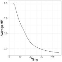
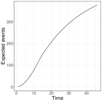
Figure 5: Average HR as a function of study duration (left) and expected event accumulation as a function of study duration (right)

To illustrate our approach, we adopt a group sequential design comprising 4 analyses conducted at the 12th, 20th, 28th, and 36th months. Additionally, we discuss three different designs: one-sided design (see Table 2), two-sided symmetric design (see Table 3), and two-sided asymmetric design (see Table 4).

From Table 2, 3, and 4, by comparing different WLR methods in different designs, we find that WLR50 commonly has a higher expected sample size and the number of events. This is because setting $\rho=0.5,\gamma=0$ in the Fleming-Harrington weight emphasizes early differences (Wu and Gilbert,, 2002). However, the discussed example has a delayed treatment effect, which leads to a relatively weaker power when applying FH(0.5, 0). In contrast, WLR05 emphasizes late differences, which is tailored to the discussed example. Thus, it gives a relatively small sample size. And the WLR55 has a sample size and the number of events in the middle of WLR05 and WLR50.

Table 2: Comparison between PH and NPH under one-sided design

Method Expected sample size Expected number of events Information fraction Standardized treatment effect Upper Bound Cumulative prob to cross upper bound under $H_{0}$ Cumulative prob to cross upper bound under $H_{1}$ 1st analysis at month 12 AHR $463.93$ $99.65$ $0.3241$ $0.1749$ $3.7670$ $0.0001$ $0.0021$ WLR05 $364.52$ $78.29$ $0.1325$ $0.6258$ $6.1754$ $0.0000$ $0.0000$ WLR50 $552.43$ $118.65$ $0.4247$ $0.1731$ $3.2685$ $0.0005$ $0.0085$ WLR55 $378.26$ $81.25$ $0.1923$ $0.6755$ $5.0459$ $0.0000$ $0.0000$ 2nd analysis at month 20 AHR $463.93$ $192.90$ $0.6226$ $0.3039$ $2.6020$ $0.0047$ $0.3023$ WLR05 $364.52$ $151.56$ $0.4091$ $0.7648$ $3.3697$ $0.0004$ $0.1168$ WLR50 $552.43$ $229.69$ $0.7446$ $0.3186$ $2.3684$ $0.0091$ $0.4087$ WLR55 $378.26$ $157.28$ $0.5212$ $0.8938$ $2.9217$ $0.0017$ $0.2288$ 3rd analysis at month 28 AHR $463.93$ $258.97$ $0.8384$ $0.3567$ $2.2209$ $0.0146$ $0.7328$ WLR05 $364.52$ $203.48$ $0.7188$ $0.7550$ $2.4274$ $0.0077$ $0.6649$ WLR50 $552.43$ $308.37$ $0.9105$ $0.3906$ $2.1470$ $0.0186$ $0.7745$ WLR55 $378.26$ $211.15$ $0.8043$ $0.9470$ $2.2716$ $0.0121$ $0.7260$ 4th analysis at month 36 AHR $463.93$ $307.39$ $1.0000$ $0.3810$ $2.0453$ $0.0250$ $0.9000$ WLR05 $364.52$ $241.52$ $1.0000$ $0.7316$ $2.0024$ $0.0250$ $0.9000$ WLR50 $552.43$ $366.03$ $1.0000$ $0.4306$ $2.0744$ $0.0250$ $0.9000$ WLR55 $378.26$ $250.63$ $1.0000$ $0.9734$ $2.0276$ $0.0250$ $0.9000$ 1 WLR05, WLR50, WLR55 refer to the WLR method with weight as FH(0, 0.5), FH(0.5), and FH(0.5, 0.5), respectively.

Table 3: Comparison between PH and NPH under a two-sided symmetric design

Method Expected sample size Expected number of events Information fraction Standardized treatment effect Upper Bound Cumulative prob to cross upper bound under $H_{0}$ Cumulative prob to cross upper bound under $H_{1}$ Lower Bound Cumulative prob to cross lower bound under $H_{0}$ Cumulative prob to cross lower bound under $H_{1}$ 1st analysis at month 12 AHR $463.93$ $99.65$ $0.3241$ $0.1749$ $3.7670$ $0.0001$ $0.0021$ $-3.7670$ $0.0001$ $0.0000$ WLR05 $364.52$ $78.29$ $0.1325$ $0.6258$ $6.1754$ $0.0000$ $0.0000$ $-6.1754$ $0.0000$ $0.0000$ WLR50 $552.43$ $118.65$ $0.4247$ $0.1731$ $3.2685$ $0.0005$ $0.0085$ $-3.2685$ $0.0005$ $0.0000$ WLR55 $378.26$ $81.25$ $0.1923$ $0.6755$ $5.0459$ $0.0000$ $0.0000$ $-5.0459$ $0.0000$ $0.0000$ 2nd analysis at month 20 AHR $463.93$ $192.90$ $0.6226$ $0.3039$ $2.6020$ $0.0047$ $0.3023$ $-2.6020$ $0.0047$ $0.0000$ WLR05 $364.52$ $151.56$ $0.4091$ $0.7648$ $3.3697$ $0.0004$ $0.1168$ $-3.3697$ $0.0004$ $0.0000$ WLR50 $552.43$ $229.70$ $0.7446$ $0.3186$ $2.3684$ $0.0091$ $0.4087$ $-2.3684$ $0.0091$ $0.0000$ WLR55 $378.26$ $157.28$ $0.5212$ $0.8938$ $2.9217$ $0.0017$ $0.2288$ $-2.9217$ $0.0017$ $0.0000$ 3rd analysis at month 28 AHR $463.93$ $258.97$ $0.8384$ $0.3567$ $2.2209$ $0.0146$ $0.7328$ $-2.2209$ $0.0146$ $0.0000$ WLR05 $364.52$ $203.48$ $0.7188$ $0.7550$ $2.4274$ $0.0077$ $0.6649$ $-2.4274$ $0.0077$ $0.0000$ WLR50 $552.43$ $308.37$ $0.9105$ $0.3906$ $2.1470$ $0.0186$ $0.7745$ $-2.1470$ $0.0186$ $0.0000$ WLR55 $378.26$ $211.15$ $0.8043$ $0.9470$ $2.2716$ $0.0121$ $0.7260$ $-2.2716$ $0.0121$ $0.0000$ 4th analysis at month 36 AHR $463.93$ $307.39$ $1.0000$ $0.3810$ $2.0453$ $0.0250$ $0.9000$ $-2.0453$ $0.0250$ $0.0000$ WLR05 $364.52$ $241.52$ $1.0000$ $0.7316$ $2.0024$ $0.0250$ $0.9000$ $-2.0024$ $0.0250$ $0.0000$ WLR50 $552.43$ $366.03$ $1.0000$ $0.4306$ $2.0744$ $0.0250$ $0.9000$ $-2.0744$ $0.0250$ $0.0000$ WLR55 $378.26$ $250.63$ $1.0000$ $0.9734$ $2.0276$ $0.0250$ $0.9000$ $-2.0276$ $0.0250$ $0.0000$ 1 WLR05, WLR50, WLR55 refer to the WLR method with weight as FH(0, 0.5), FH(0.5), and FH(0.5, 0.5), respectively.

Table 4: Comparison between PH and NPH under a two-sided asymmetric design

Method Expected sample size Expected number of events Information fraction Standardized treatment effect Upper Bound Cumulative prob to cross upper bound under $H_{0}$ Cumulative prob to cross upper bound under $H_{1}$ Lower Bound Cumulative prob to cross lower bound under $H_{0}$ Cumulative prob to cross lower bound under $H_{1}$ 1st analysis at month 12 AHR $501.16$ $107.64$ $0.3241$ $0.1749$ $3.7670$ $0.0001$ $0.0023$ $-1.2905$ $0.0984$ $0.0147$ WLR05 $386.87$ $83.10$ $0.1325$ $0.6258$ $6.1754$ $0.0000$ $0.0000$ $-1.5483$ $0.0608$ $0.0048$ WLR50 $605.29$ $130.01$ $0.4247$ $0.1731$ $3.2685$ $0.0005$ $0.0094$ $-1.1165$ $0.1321$ $0.0210$ WLR55 $405.93$ $87.19$ $0.1923$ $0.6755$ $5.0459$ $0.0000$ $0.0000$ $-1.4040$ $0.0802$ $0.0074$ 2nd analysis at month 20 AHR $501.16$ $208.38$ $0.6226$ $0.3039$ $2.6020$ $0.0047$ $0.3315$ $0.3040$ $0.6211$ $0.0391$ WLR05 $386.87$ $160.86$ $0.4091$ $0.7648$ $3.3697$ $0.0004$ $0.1302$ $0.1103$ $0.5484$ $0.0199$ WLR50 $605.29$ $251.67$ $0.7446$ $0.3186$ $2.3684$ $0.0091$ $0.4479$ $0.5371$ $0.7053$ $0.0538$ WLR55 $405.93$ $168.78$ $0.5212$ $0.8938$ $2.9217$ $0.0017$ $0.2531$ $0.2801$ $0.6139$ $0.0288$ 3rd analysis at month 28 AHR $501.16$ $279.75$ $0.8384$ $0.3567$ $2.2209$ $0.0146$ $0.7656$ $1.3322$ $0.9100$ $0.0685$ WLR05 $386.87$ $215.95$ $0.7188$ $0.7550$ $2.4274$ $0.0077$ $0.6943$ $1.1901$ $0.8901$ $0.0503$ WLR50 $605.29$ $337.87$ $0.9105$ $0.3906$ $2.1470$ $0.0186$ $0.8088$ $1.5020$ $0.9337$ $0.0811$ WLR55 $405.93$ $226.59$ $0.8043$ $0.9470$ $2.2716$ $0.0121$ $0.7568$ $1.3277$ $0.9119$ $0.0626$ 4th analysis at month 36 AHR $501.16$ $332.06$ $1.0000$ $0.3810$ $2.0453$ $0.0243$ $0.9000$ $2.0429$ $0.9756$ $0.1004$ WLR05 $386.87$ $256.33$ $1.0000$ $0.7316$ $2.0024$ $0.0224$ $0.9000$ $2.0024$ $0.9776$ $0.1001$ WLR50 $605.29$ $401.05$ $1.0000$ $0.4306$ $2.0744$ $0.0247$ $0.9000$ $2.0736$ $0.9753$ $0.1000$ WLR55 $405.93$ $268.96$ $1.0000$ $0.9734$ $2.0276$ $0.0234$ $0.9000$ $2.0276$ $0.9766$ $0.1001$ 1 WLR05, WLR50, WLR55 refer to the WLR method with weight as FH(0, 0.5), FH(0.5), and FH(0.5, 0.5), respectively.

6 Discussion

Group sequential design has been widely used in clinical trials, particularly for time-to-event endpoints. Recent results from immunotherapy-based oncology trials have highlighted the presence of non-proportional hazards. Thoroughly assessing NPH scenarios during the trial design stage becomes paramount to evaluate risks and benefits. This paper undertakes a comprehensive exploration of three commonly employed NPH methods for group sequential design. These methodologies have been seamlessly integrated into the gsDesign2 R package, which can be conveniently accessed at https://merck.github.io/gsDesign2/. Furthermore, our ongoing efforts involve expanding the functionality of the R package to design stratified clinical trials under NPH. Additionally, we are actively developing a shiny app that promises to further streamline trial design.

Appendix A

A.1 Deriving of the asymptotic distribution of $Z^{(\text{ahr})}$ in Section 2.1

Define

$$B_{k}=\sqrt{t_{k}}Z_{k},$$

with $t_{k}=\mathcal{I}_{k,H_{0}}/\mathcal{I}_{k,H_{1}}$. Considering

$$\begin{array}[]{ll}E(Z_{k}^{(\text{ahr})}|H_{0})=0,&\text{Var}(Z_{k}^{(\text{ahr})}|H_{0})=1\\ E(Z_{k}^{(\text{ahr})}|H_{1})=\theta_{k}\sqrt{\mathcal{I}_{k,H_{0}}},&\text{Var}(Z_{k}^{(\text{ahr})}|H_{1})=\mathcal{I}_{k,H_{0}}/\mathcal{I}_{k,H_{1}}.\end{array},$$

we have

$$\begin{array}[]{ll}E(B_{k}|H_{0})=0,&\text{Var}(B_{k}|H_{0})=t_{k}\\ E(B_{k}|H_{1})=\theta_{k}t_{k}\sqrt{\mathcal{I}_{k,H_{0}}},&\text{Var}(B_{k}|H_{1})=t_{k}\mathcal{I}_{k,H_{0}}/\mathcal{I}_{k,H_{1}}.\end{array}$$

We assume independent increments in the B-process (Proschan et al.,, 2006), then we immediately have

$$\begin{array}[]{l}\text{Cov}(B_{i},B_{j}|H_{0})=\text{Var}(B_{i}|H_{0})=t_{i},\\ \text{Cov}(B_{i},B_{j}|H_{1})=\text{Var}(B_{i}|H_{1})=t_{i}\mathcal{I}_{i,H_{0}}/\mathcal{I}_{i,H_{1}}.\end{array}$$

Given the closed-form correlation between $B_{k}$ and $Z_{k}$, we have

$$\text{Cov}(Z_{i},Z_{j})=\text{Cov}(B_{i}/\sqrt{t_{i}},B_{j}/\sqrt{t_{j}})=\frac{1}{\sqrt{t_{i}t_{j}}}\text{Cov}(B_{i},B_{j})=\frac{1}{\sqrt{t_{i}t_{j}}}\text{Var}(B_{i})$$

for $1\leq i\leq j\leq K$. So we have

$$\text{Cov}(Z_{i},Z_{j}|H_{0})=\sqrt{\frac{t_{i}}{t_{j}}},\text{Cov}(Z_{i},Z_{j}|H_{1})=\sqrt{\frac{t_{i}}{t_{j}}}\frac{\mathcal{I}_{i,H_{0}}}{\mathcal{I}_{i,H_{1}}}.$$

A.2 Deriving the asymptotic distribution of the log HR under the piecewise model in Section 2.1

The likelihood of $\lambda_{i,m}$ is

$$L(\lambda_{i,m})=\exp(-\lambda_{i,m}T_{i,m})\;\lambda_{i,m}^{d_{i,m}},$$

where $d_{i,m}$ is the number of observed events in $(t_{m-1},t_{m}]$ and $T_{i,m}$ is the follow-up time (total time on test) in $(t_{m-1},t_{m}]$. If we denote the above likelihood function of $\lambda_{i,m}$ can be re-written into the likelihood function of $\gamma_{i,m}$, i.e.,

$$L(\gamma_{i,m})=\exp(-e^{\gamma_{i,m}}T_{i,m})\;e^{\gamma_{i,m}d_{i,m}}.$$

This leads to a log-likelihood:

$$\ell(\gamma_{i,m})\triangleq\log\left(L(\gamma_{i,m})\right)=-e^{\gamma_{i,m}}T_{i,m}+\gamma_{i,m}d_{i,m}.$$

By setting its first derivative with respect to $\gamma_{i,m}$ as zero,

$$\frac{\partial}{\partial\gamma_{i,m}}\ell(\gamma_{i,m})=-e^{\gamma_{i,m}}T_{i,m}+d_{i,m}=0$$

one gets its maximum likelihood estimation as

$$\hat{\gamma}_{i,m}=\log(d_{i,m}/T_{i,m}).$$ (7)

By taking the second derivative of $\ell(\gamma_{i,m})$, one gets the variance of $\hat{\gamma}_{i,m}$ as

$$\widehat{\text{Var}(\hat{\gamma}_{i,m})}=\left(-\frac{\partial^{2}}{\partial\gamma_{i,m}^{2}}\ell(\hat{\gamma}_{i,m})\right)^{-1}=\left(e^{\hat{\gamma}_{i,m}}T_{i,m}\right)^{-1}=\frac{1}{d_{i,m}}.$$

By using the delta method, we get the asymptotic distribution of $\widehat{\lambda}_{i,m}$ as

$$\log(\widehat{\lambda}_{i,m})\overset{\cdot}{\sim}\text{Normal}\left(\log(\lambda_{i,m}),\;1/d_{i,m}\right),\;\;\forall i\in\{0,1\}$$ (8)

Accordingly, one can estimate

$$\beta_{m}=\log\left(\frac{\lambda_{1,m}}{\lambda_{0,m}}\right)=\log(\lambda_{1,m})-\log(\lambda_{0,m}).$$ (9)

as

$$\widehat{\beta}_{m}=\log\left(\frac{\widehat{\lambda}_{1,m}}{\widehat{\lambda}_{0,m}}\right)=\log(\lambda_{1,m})-\log(\lambda_{0,m}).$$

For both $\lambda_{1,m}$ and $\lambda_{0,m}$ above, by equation (7), we know they can be estimated by

$$\widehat{\lambda}_{i,m}=\frac{d_{i,m}}{T_{i,m}},\;\;\forall i\in\{0,1\}$$

where $d_{0,m},d_{1,m}$ are number of events in $(t_{m-1},t_{m}]$ for group $0,1$, respectively.

By plugging the asymptotic distribution of $\{\lambda_{0,m},\lambda_{1,m}\}$ in equation (8) into (9), we can derive the asymptotic distribution of $\beta_{m}$:

$$\widehat{\beta}_{m}\overset{\cdot}{\sim}\text{Normal}\left(\beta_{m},\frac{1}{d_{0,m}}+\frac{1}{d_{1,m}}\right)\;\;\forall m=1,\ldots,M.$$ (10)

A.3 Deriving the average HR by the WLR test in Section 2.4

For the second term in (4), it is essentially a Harmonic mean

$$\frac{p_{0,k}\pi_{0,k}(s)\;p_{1,k}\pi_{1,k}(s)}{\pi(s)}=1\bigg{/}\left[\frac{1}{p_{0,k}\pi_{0,k}(s)}+\frac{1}{p_{1,k}\pi_{1,k}(s)}\right],$$

which is used to weigh the difference between hazards.

From (4), we have

$$\Delta_{k} = \int_{0}^{\tau_{k}}w(s)\frac{p_{0,k}\pi_{0,k}(s)\;p_{1,k}\pi_{1,k}(s)}{\pi_{k}(s)}\left[\lambda_{1}(s)-\lambda_{0}(s)\right]ds$$ (11)

$$= \int_{0}^{\tau_{k}}w(s)\frac{p_{0,k}\pi_{0,k}(s)\;p_{1,k}\pi_{1,k}(s)}{\pi_{k}(s)^{2}}\underbrace{\left[\lambda_{1}(s)-\lambda_{0}(s)\right]\pi_{k}(s)}_{\mathcal{A}}ds.$$

For $\mathcal{A}$, one has

$$\mathcal{A} = \left[\lambda_{1}(s)-\lambda_{0}(s)\right][p_{0}\pi_{0,k}+p_{1}\pi_{1,k}(s)]$$

$$= \left[\lambda_{1}(s)-\lambda_{0}(s)\right]p_{0}\pi_{0,k}(s)+\left[\lambda_{1}(s)-\lambda_{0}(s)\right]p_{1}\pi_{1,k}(s)$$

$$= \left[\frac{\lambda_{1}(s)}{\lambda_{0}(s)}-1\right]\lambda_{0}(s)p_{0}\pi_{0,k}(s)+\left[1-\frac{\lambda_{0}(s)}{\lambda_{1}(s)}\right]\lambda_{1}(s)p_{1}\pi_{1,k}(s)$$

By plugging $x=\log(\lambda_{1}(s)/\lambda_{0}(s))$ and $x=\log(\lambda_{0}(s)/\lambda_{1}(s))$ expansion $e^{x}\approx 1+x$, we get

$$\left\{\begin{array}[]{c}\frac{\lambda_{1}(s)}{\lambda_{0}(s)}=1+\log\left(\frac{\lambda_{1}(s)}{\lambda_{0}(s)}\right)\\ \frac{\lambda_{0}(s)}{\lambda_{1}(s)}\approx 1-\log\left(\frac{\lambda_{1}(s)}{\lambda_{0}(s)}\right)\end{array}\right..$$

If one plugs in the above Taylor expansion into $\mathcal{A}$, one can approximate $\mathcal{A}$ by

$$\mathcal{A} = \log\left(\frac{\lambda_{1}(s)}{\lambda_{0}(s)}\right)p_{0}\pi_{0,k}(s)\lambda_{0}(s)+\log\left(\frac{\lambda_{1}(s)}{\lambda_{0}(s)}\right)p_{1}\pi_{1,k}(s)\lambda_{1}(s)+O(1/n)$$

$$\approx \log\left(\frac{\lambda_{1}(s)}{\lambda_{0}(s)}\right)\left[p_{0}\pi_{0,k}(s)\lambda_{0}(s)+p_{1}\pi_{1,k}(s)\lambda_{1}(s)\right]$$

$$= \log\left(\frac{\lambda_{1}(s)}{\lambda_{0}(s)}\right)v^{\prime}(s)$$

So, we can simplify (11) into

$$\Delta_{k}\approx\int_{0}^{\tau_{k}}w(s)\frac{p_{0,k}\pi_{0,k}(s)\;p_{1,k}\pi_{1,k}(s)}{\pi_{k}(s)^{2}}\log\left(\frac{\lambda_{1}(s)}{\lambda_{0}(s)}\right)v^{\prime}(s)ds.$$

By normalizing the weights of $\log\left(\frac{\lambda_{1}(s)}{\lambda_{0}(s)}\right)$, we have the conclusion in Section 3.

A.4 Deriving the bridge from $\beta^{\text{(ahr)}}$ to $\beta^{\text{(wlr)}}$ in Section 2.4

Notice the above $\Delta_{k}$ in (4) takes the integration from 0 to the $k$-th analysis at time $\tau_{k}$. If it is at the end of the study, we have decomposed $\Delta_{K}$ – via the piecewise model – as

$$\Delta_{K} \approx \sum_{\ell=1}^{M}\int_{\dot{\tau}_{\ell-1}}^{\dot{\tau}_{\ell}}w(s)\frac{p_{0,\ell}\pi_{0,\ell}(s)\;p_{1,\ell}\pi_{1,\ell}(s)}{\pi_{\ell}(s)^{2}}\log\left(\frac{\lambda_{1}(s)}{\lambda_{0}(s)}\right)v^{\prime}(s)ds$$

$$= \sum_{\ell=1}^{M}\int_{\dot{\tau}_{\ell-1}}^{\dot{\tau}_{\ell}}w(s)\frac{p_{0,\ell}\pi_{0,\ell}(s)\;p_{1,\ell}\pi_{1,\ell}(s)}{\pi_{\ell}(s)^{2}}\beta_{\ell}\;v^{\prime}(s)ds$$

$$= \sum_{\ell=1}^{M}\beta_{\ell}\;\int_{\dot{\tau}_{\ell-1}}^{\dot{\tau}_{\ell}}w(s)\frac{p_{0,\ell}\pi_{0,\ell}(s)\;p_{1,\ell}\pi_{1,\ell}(s)}{\pi_{\ell}(s)^{2}}v^{\prime}(s)ds$$

If we further assume the dropout rate in the two arms is the same, then we have $\pi_{0}(s)=\pi_{1}(s)=\pi(s)$ under the local alternatives (Section 2.3 Yung and Liu,, 2020). In this way, $\Delta_{k}$ can be simplified into

$$\Delta_{K} \approx \sum_{\ell=1}^{M}\beta_{\ell}\;p_{0,\ell}\;p_{1,\ell}\int_{\dot{\tau}_{\ell-1}}^{\dot{\tau}_{\ell}}w(s)\;v^{\prime}(s)ds$$

When $w(s)=\frac{\left(\frac{1}{1/d_{0,\ell}+1/d_{1,\ell}}\right)^{-1}}{p_{0,\ell}p_{1,\ell}d_{\ell}\sum_{i=1}^{M}\left(\frac{1}{1/d_{0,i}+1/d_{1,i}}\right)^{-1}}$ when $s\in[\dot{\tau}_{\ell-1},\dot{\tau}_{\ell})$, then we have

$$\Delta_{K} \approx \sum_{\ell=1}^{M}\beta_{\ell}\;p_{0,\ell}\;p_{1,\ell}\int_{\dot{\tau}_{\ell-1}}^{\dot{\tau}_{\ell}}\frac{\left(\frac{1}{1/d_{0,\ell}+1/d_{1,\ell}}\right)^{-1}}{p_{0,\ell}p_{1,\ell}d_{\ell}\sum_{i=1}^{M}\left(\frac{1}{1/d_{0,i}+1/d_{1,i}}\right)^{-1}}\;v^{\prime}(s)ds$$

$$= \sum_{\ell=1}^{M}\beta_{\ell}\;p_{0,\ell}\;p_{1,\ell}\frac{\left(\frac{1}{1/d_{0,\ell}+1/d_{1,\ell}}\right)^{-1}}{p_{0,\ell}p_{1,\ell}d_{\ell}\sum_{i=1}^{M}\left(\frac{1}{1/d_{0,i}+1/d_{1,i}}\right)^{-1}}\int_{\tau_{\ell-1}}^{\tau_{\ell}}v^{\prime}(s)ds$$

$$= \sum_{\ell=1}^{M}\beta_{\ell}\;p_{0,\ell}\;p_{1,\ell}\frac{\left(\frac{1}{1/d_{0,\ell}+1/d_{1,\ell}}\right)^{-1}}{p_{0,\ell}p_{1,\ell}d_{\ell}\sum_{i=1}^{M}\left(\frac{1}{1/d_{0,i}+1/d_{1,i}}\right)^{-1}}[v(\tau_{\ell})-v(\tau_{\ell-1})]$$

$$= \sum_{\ell=1}^{M}\beta_{\ell}\;p_{0,\ell}\;p_{1,\ell}\frac{\left(\frac{1}{1/d_{0,\ell}+1/d_{1,\ell}}\right)^{-1}}{p_{0,\ell}p_{1,\ell}d_{\ell}\sum_{i=1}^{M}\left(\frac{1}{1/d_{0,i}+1/d_{1,i}}\right)^{-1}}d_{\ell}$$

$$= \sum_{\ell=1}^{M}\beta_{\ell}\frac{\left(\frac{1}{1/d_{0,\ell}+1/d_{1,\ell}}\right)^{-1}}{\sum_{i=1}^{M}\left(\frac{1}{1/d_{0,i}+1/d_{1,i}}\right)^{-1}}$$

where $d_{\ell}$ is the expected number of events at time $[\tau_{\ell-1},\tau_{\ell})$. The logarithm of AHR can be calculated after normalizing the weights in $\Delta_{K}$, i.e.,

$$\beta \approx \frac{\sum_{\ell=1}^{M}\beta_{\ell}\frac{\left(\frac{1}{1/d_{0,\ell}+1/d_{1,\ell}}\right)^{-1}}{\sum_{i=1}^{M}\left(\frac{1}{1/d_{0,i}+1/d_{1,i}}\right)^{-1}}}{\sum_{\ell=1}^{M}\frac{\left(\frac{1}{1/d_{0,\ell}+1/d_{1,\ell}}\right)^{-1}}{\sum_{i=1}^{M}\left(\frac{1}{1/d_{0,i}+1/d_{1,i}}\right)^{-1}}}$$

$$= \sum_{\ell=1}^{M}\beta_{\ell}\frac{\left(\frac{1}{1/d_{0,\ell}+1/d_{1,\ell}}\right)^{-1}}{\sum_{i=1}^{M}\left(\frac{1}{1/d_{0,i}+1/d_{1,i}}\right)^{-1}}.$$

This is the formula to derive $\beta^{\text{(ahr)}}$.

A.5 Deriving the expected number of events in the AHR test in Section 3.3

Proof 1

The key count we consider is the expected events in each time interval. Specifically, it is the number of subjects with events in the interval $(\tau_{m-1},\tau_{m}]$, which is denoted as $\bar{n}(\tau_{m-1},\tau_{m})$ for any $m=1,\ldots,M$. We focus on the expected value of $\bar{n}(\tau_{m-1},\tau_{m})$ due to its usefulness in computing an average hazard ratio under the piecewise model, which is calculated as

$$E\left(\bar{n}(\tau_{m-1},\tau_{m})\right)=\int_{0}^{\tau-{\tau_{m-1}}}g(u)P\left(\tau_{m-1}<T\leq\min(\tau_{m},\tau-u),\;T\leq C\right)du$$ (12)

Here the random variable $T>0$ denotes the subject time of an individual until an event. And random variable $C>0$ denotes the subject time of an individual until loss-to-follow-up. Please note that $T,C$ are defined by $\{\widetilde{T}_{m},\widetilde{C}_{m}\}_{m=1,\ldots,M}$, i.e.,

$$T=\sum_{m=1}^{M}\min\{T_{m},\tau_{m},\tau_{m-1}\}\prod_{j=1}^{m-1}\mathbbm{1}\{T_{j}>\tau_{j}-\tau_{j-1}\}$$

$$C=\sum_{m=1}^{M}\min\{C_{m},\tau_{m},\tau_{m-1}\}\prod_{j=1}^{m-1}\mathbbm{1}\{C_{j}>\tau_{j}-\tau_{j-1}\}.$$

The integration in (12) sums subjects enrolled before time $\tau-\tau_{m-1}$. This is because, for a subject to be in the count $\bar{n}(\tau_{m-1},\tau_{m})$, they must be enrolled prior to time $\tau-\tau_{m-1}$. By dividing the integration interval $\int_{0}^{\tau-\tau_{m-1}}$ into two sub-intervals, i.e., $\int_{0}^{\tau-\tau_{m}}$ and $\int_{\tau-\tau_{m}}^{\tau-\tau_{m-1}}$, we can simplify equation (12) as

$$E\left(\bar{n}(\tau_{m-1},\tau_{m})\right)$$

$$= \int_{0}^{\tau-\tau_{m}}g(u)P\left(\tau_{m-1}<T\leq\tau_{m},T\leq C\right)du+$$

$$\int_{\tau-\tau_{m}}^{\tau-\tau_{m-1}}g(u)P\left(\tau_{m-1}<T\leq\tau-u,T\leq C\right)du$$

$$= \underbrace{G(\tau-\tau_{m})}_{\mathcal{A}}\underbrace{P\left(\tau_{m-1}<T\leq\tau_{m},T\leq C\right)}_{\mathcal{B}}+$$

$$\underbrace{\int_{\tau-\tau_{m}}^{\tau-\tau_{m-1}}g(u)P\left(\tau_{m-1}<T\leq\tau-u,T\leq C\right)du}_{\mathcal{C}}$$

• For $\mathcal{A}$ in (1), it can be simplified into

  $$\mathcal{A}=G_{M+1-m}\triangleq G(\tau_{M+1-m}).$$

  This is because $g(u)=\gamma_{j}$ when $u\in(\tau_{j-1},\tau_{j}]$, one has

  $$G_{j}\triangleq G(\tau_{j})=G_{j-1}+\gamma_{j}(\tau_{j}-\tau_{j-1})$$

  with $G_{0}=0$.

• For $\mathcal{B}$ in (1), it can be simplified into

  $$\mathcal{B}\triangleq d_{m}= = \underbrace{P(\min\{T,C\}>\tau_{m-1})}_{Q_{m-1}}P(0<T_{m}\leq\tau_{m}-\tau_{m-1},T_{m}\leq C_{m})$$

  $$= Q_{m-1}\left(1-e^{-(\lambda_{m}+\eta_{m})(\tau_{m}-\tau_{m-1})}\right)\frac{\lambda_{m}}{\lambda_{m}+\eta_{m}}$$

  For $Q_{m-1}$, one has

  $$Q_{m-1}=\prod_{j=1}^{m-1}\underbrace{P(\min\{T_{m},Y_{m}\}>\tau_{m-1})}_{q_{m}}=\prod_{j=1}^{m-1}e^{-(\lambda_{m-1}+\eta_{m-1})(\tau_{m-1}-\tau_{m-2})}.$$

• For $\mathcal{C}$ in (1), by transferring $u$ into $v=u-\tau+\tau_{m}$, it can be simplified as

  $$\mathcal{C} = \int_{0}^{\tau_{m}-\tau_{m-1}}g(v+\tau-\tau_{m})P\left(\tau_{m-1}<T\leq\tau_{m}-v,T\leq C\right)dv$$

  $$= \gamma_{M+1-m}\int_{0}^{\tau_{m}-\tau_{m-1}}P\left(\tau_{m-1}<T\leq\tau_{m}-v,T\leq C\right)dv$$

  $$= \gamma_{M+1-m}P(\min\{T,C\}>\tau_{m-1})\int_{0}^{\tau_{m}-\tau_{m-1}}P\left(T_{m}\leq v,T_{m}\leq C_{m}\right)dv$$

  $$= \gamma_{M+1-m}Q_{m-1}\frac{\lambda_{m}}{\lambda_{m}+\eta_{m}}\int_{0}^{\tau_{m}-\tau_{m-1}}\left(1-e^{-(\lambda_{m}+\eta_{m})v}\right)dv$$

  $$= \gamma_{M+1-m}Q_{m-1}\frac{\lambda_{m}}{\lambda_{m}+\eta_{m}}\left(\tau_{m}-\tau_{m-1}-\frac{1-e^{-(\lambda_{m}+\eta_{m})(\tau_{m}-\tau_{m-1})}}{\lambda_{m}+\eta_{m}}\right)$$

  $$= \gamma_{M+1-m}Q_{m-1}\frac{\lambda_{m}}{\lambda_{m}+\eta_{m}}\left(\tau_{m}-\tau_{m-1}-\frac{1-q_{m}}{\lambda_{m}+\eta_{m}}\right)$$

By combining $\mathcal{A},\mathcal{B},\mathcal{C}$ together, we can simplify (1) as

$$E\left(\bar{n}(\tau_{m-1},\tau_{m})\right)=G_{M+1-m}d_{m}+\frac{\lambda_{m}Q_{m-1}\gamma_{M+1-m}}{\lambda_{m}+\eta_{m}}\left(\tau_{m}-\tau_{m-1}-\frac{1-q_{m}}{\lambda_{m}+\eta_{m}}\right)$$

A.6 Local alternative assumption in Section 2.2

Notice that the asymptotic variance of $Z_{k}^{\text{(wlr)}}$ in Section 2.2 is $\widetilde{\sigma}^{2}_{b,k}/\sigma_{k}^{2}$. And in the existing literature, there are multiple proposals to simplify it.

• A common assumption is called local alternative (Schoenfeld,, 1981; Barthel et al.,, 2006; Hasegawa,, 2014). It assumes $\sup_{t<\tau}|\log\left[\lambda_{1}(t)/\lambda_{0}(t)\right]|=O(n^{-1/2}),$ and this assumption makes the asymptotic variance $\widetilde{\sigma}_{b,k}^{2}/\sigma_{k}^{2}$ in Section 2.2 equal to $1+o(n^{-1/2})$. Thus, an alternative approximation for the large-sample distribution of $Z_{k}^{(\text{wlr})}$ is

  $$Z_{k}^{(\text{wlr})}\overset{d}{\to}N\left(\sqrt{n_{k}}\theta_{k},1\right).$$

• Another assumption is called fixed alternative. An example of a fixed alternative is the PH. Under the fixed alternative, $\widetilde{\sigma}^{2}_{b}/\sigma_{k}^{2}$ and 1 may both serve as approximations for the large-sample variance of $Z_{k}^{\text{(wlr)}}$, but none of them are the limiting variance of $Z_{k}^{\text{(wlr)}}$. Consequently, there is no guarantee that one is always more accurate than the others. Additionally, the convergence in distribution for $Z_{k}^{\text{(wlr)}}$ itself requires the assumption of local alternatives, so we do not recommend using the fixed alternative.

• In the literature, we also find the existence of distant alternative. This assumption lies in the ART module in Stata by Barthel et al., (2006). Basically, it approximates the asymptotic variance of $U_{k}$ by simulations. In this paper, we use local alternatives.

A.7 Calculation details of Example 4

At the second analysis, the upper bound $b_{2}$ is the solved from

$$\alpha(t_{2})-\alpha(t_{1})=\text{Pr}\left(Z_{1}^{(\text{mc})}<b_{1},Z_{2}^{(\text{mc})}\geq b_{2}\;|\;H_{0}\right).$$

And the right-hand side can be further simplified as

$$\begin{array}[]{lllll}&&\alpha(t_{2})-\alpha(t_{1})\\ &=&\text{Pr}\left(Z_{1}^{(\text{mc})}<b_{1},Z_{2}^{(\text{mc})}\geq b_{2}\;|\;H_{0}\right)\\ &=&\text{Pr}\left(Z_{1}^{(\text{mc})}<b_{1}\;|\;H_{0}\right)-\text{Pr}\left(Z_{1}^{(\text{mc})}<b_{1},Z_{2}^{(\text{mc})}<b_{2}\;|\;H_{0}\right)\\ &=&\text{Pr}\left(Z_{1}^{(\text{mc})}<b_{1}\;|\;H_{0}\right)-\\ &&\text{Pr}\left(\max\left\{Z_{1}^{(\text{wlr}_{1})},\ldots,Z_{1}^{(\text{wlr}_{L})}\right\}<b_{1},\max\left\{Z_{2}^{(\text{wlr}_{1})},\ldots,Z_{2}^{(\text{wlr}_{L})}\right\}<b_{2}\;|\;H_{0}\right)\\ &=&\text{Pr}\left(Z_{1}^{(\text{mc})}<b_{1}\;|\;H_{0}\right)-\text{Pr}\left(\cap_{\ell=1}^{L}Z_{1}^{(\text{wlr}_{\ell})}<b_{1},\;\cap_{\ell=1}^{L}Z_{2}^{(\text{wlr}_{\ell})}<b_{2}\;|\;H_{0}\right).\\ \end{array}$$

Generally, at the $k$-th analysis ($2\leq k\leq K$), we have the upper bound $b_{k}$ by solving

$$\alpha(t_{k})-\alpha(t_{k-1})$$

$$= \text{Pr}\left(\cap_{i=1}^{k-1}Z_{i}^{(\text{mc})}<b_{i},Z_{k}^{(\text{mc})}\geq b_{k}\;|\;H_{0}\right)$$

$$= \text{Pr}\left(\cap_{i=1}^{k-1}Z_{i}^{(\text{mc})}<b_{i}\;|\;H_{0}\right)-\text{Pr}\left(\cap_{i=1}^{k}Z_{i}^{(\text{mc})}<b_{i}\;|\;H_{0}\right)$$

$$= \text{Pr}\left(\cap_{i=1}^{k-1}\max\left\{Z_{i}^{(\text{wlr}_{1})},\ldots,Z_{i}^{(\text{wlr}_{L})}\right\}<b_{i}\;|\;H_{0}\right)-$$

$$\text{Pr}\left(\cap_{i=1}^{k}\max\left\{Z_{i}^{(\text{wlr}_{1})},\ldots,Z_{i}^{(\text{wlr}_{L})}\right\}<b_{i}\;|\;H_{0}\right)$$

$$= \text{Pr}\left(\cap_{i=1}^{k-1}\cap_{\ell=1}^{L}Z_{i}^{(\text{wlr}_{\ell})}<b_{i}\;|\;H_{0}\right)-\text{Pr}\left(\cap_{i=1}^{k}\cap_{\ell=1}^{L}Z_{i}^{(\text{wlr}_{\ell})}<b_{i}\;|\;H_{0}\right)$$

A.8 Compute the probability to cross the upper bound at the third analysis by MaxCombo test

Following Example 3 and 4 with known $a_{1},a_{2},a_{3},b_{1},b_{2}$ and $b_{3}$, the crossing probability is

$$\text{Pr}(a_{1}<Z_{1}^{(\text{mc})}<b_{1},a_{2}<Z_{2}^{(\text{mc})}<b_{2},Z_{3}^{(\text{mc})}>b_{3}\mid H_{1})$$

$$= \text{Pr}(a_{1}<Z_{1}^{(\text{mc})}<b_{1},a_{2}<Z_{2}^{(\text{mc})}<b_{2}\mid H_{1})-\text{Pr}(a_{1}<Z_{1}^{(\text{mc})}<b_{1},a_{2}<Z_{2}^{(\text{mc})}<b_{2},Z_{3}^{(\text{mc})}\leq b_{3}\mid H_{1})$$

$$= \left[\text{Pr}(Z_{1}^{(\text{mc})}<b_{1},Z_{2}^{(\text{mc})}<b_{2})-\text{Pr}(Z_{1}^{(\text{mc})}<a_{1},Z_{2}^{(\text{mc})}<b_{2})-\text{Pr}(Z_{1}^{(\text{mc})}<b_{1},Z_{2}^{(\text{mc})}<a_{2})+\right.$$

$$\left.\text{Pr}(Z_{1}^{(\text{mc})}<a_{1},Z_{2}^{(\text{mc})}<a_{2})\right]-\left[\text{Pr}(Z_{1}^{(\text{mc})}<b_{1},Z_{2}^{(\text{mc})}<b_{2},Z_{3}^{(\text{mc})}<b_{3})-\right.$$

$$\left.\text{Pr}(Z_{1}^{(\text{mc})}<b_{1},Z_{2}^{(\text{mc})}<a_{2},Z_{3}^{(\text{mc})}<b_{3})-\text{Pr}(Z_{1}^{(\text{mc})}<a_{1},Z_{2}^{(\text{mc})}<b_{2},Z_{3}^{(\text{mc})}<b_{3})+\right.$$

$$\left.\text{Pr}(Z_{1}^{(\text{mc})}<a_{1},Z_{2}^{(\text{mc})}<a_{2},Z_{3}^{(\text{mc})}<b_{3})\right]$$

$$= \text{Pr}(Z_{1}^{(\text{mc})}<a_{1},Z_{2}^{(\text{mc})}<a_{2})-\text{Pr}(Z_{1}^{(\text{mc})}<a_{1},Z_{2}^{(\text{mc})}<b_{2})-\text{Pr}(Z_{1}^{(\text{mc})}<b_{1},Z_{2}^{(\text{mc})}<a_{2})+$$

$$\text{Pr}(Z_{1}^{(\text{mc})}<b_{1},Z_{2}^{(\text{mc})}<b_{2})+\text{Pr}(Z_{1}^{(\text{mc})}<b_{1},Z_{2}^{(\text{mc})}<a_{2},Z_{3}^{(\text{mc})}<b_{3})+$$

$$\text{Pr}(Z_{1}^{(\text{mc})}<a_{1},Z_{2}^{(\text{mc})}<b_{2},Z_{3}^{(\text{mc})}<b_{3})-\text{Pr}(Z_{1}^{(\text{mc})}<a_{1},Z_{2}^{(\text{mc})}<a_{2},Z_{3}^{(\text{mc})}<b_{3})-$$

$$\text{Pr}(Z_{1}^{(\text{mc})}<b_{1},Z_{2}^{(\text{mc})}<b_{2},Z_{3}^{(\text{mc})}<b_{3})$$

Tables

Appendix A. Placeholder

References

- Barthel et al., (2006) Barthel, F.-S., Babiker, A., Royston, P., and Parmar, M. (2006). Evaluation of sample size and power for multi-arm survival trials allowing for non-uniform accrual, non-proportional hazards, loss to follow-up and cross-over. Statistics in medicine, 25(15):2521–2542.
- Bautista and Anderson, (2021) Bautista, O. and Anderson, K. (2021). Sample size estimation and power analysis: Time to event data. In Handbook of Statistical Methods for Randomized Controlled Trials, pages 275–300. Chapman and Hall/CRC.
- Demets and Lan, (1994) Demets, D. L. and Lan, K. G. (1994). Interim analysis: the alpha spending function approach. Statistics in medicine, 13(13-14):1341–1352.
- Fine, (2007) Fine, G. D. (2007). Consequences of delayed treatment effects on analysis of time-to-event endpoints. Drug information journal: DIJ/Drug Information Association, 41(4):535–539.
- Gehan, (1965) Gehan, E. A. (1965). A generalized wilcoxon test for comparing arbitrarily singly-censored samples. Biometrika, 52(1-2):203–224.
- Harrington et al., (1984) Harrington, D., Fleming, T., and Green, S. (1984). Procedures for serial testing in censored survival data. In Strukturen und Prozesse Neue Ansätze in der Biometrie: 28. Biometrisches Kolloquium der Biometrischen Gesellschaft Aachen, 16.–19. März 1982 Proceedings, pages 124–138. Springer.
- Harrington and Fleming, (1982) Harrington, D. P. and Fleming, T. R. (1982). A class of rank test procedures for censored survival data. Biometrika, 69(3):553–566.
- Hasegawa, (2014) Hasegawa, T. (2014). Sample size determination for the weighted log-rank test with the fleming–harrington class of weights in cancer vaccine studies. Pharmaceutical statistics, 13(2):128–135.
- Jennison and Turnbull, (2000) Jennison, C. and Turnbull, B. W. (2000). Group Sequential Methods with Applications to Clinical Trials. Chapman and Hall/CRC, Boca Raton, FL.
- Kalbfleisch and Prentice, (1981) Kalbfleisch, J. D. and Prentice, R. L. (1981). Estimation of the average hazard ratio. Biometrika, 68(1):105–112.
- Karadeniz et al., (2017) Karadeniz, P. G., Ercan, I., et al. (2017). Examining tests for comparing survival curves with right censored data. Stat Transit, 18(2):311–28.
- Karrison, (2016) Karrison, T. G. (2016). Versatile tests for comparing survival curves based on weighted log-rank statistics. The Stata Journal, 16(3):678–690.
- Lachin and Foulkes, (1986) Lachin, J. M. and Foulkes, M. A. (1986). Evaluation of sample size and power for analyses of survival with allowance for nonuniform patient entry, losses to follow-up, noncompliance, and stratification. Biometrics, 42:507–519.
- Lan and DeMets, (1983) Lan, K. K. G. and DeMets, D. L. (1983). Discrete sequential boundaries for clinical trials. Biometrika, 70:659–663.
- Lee, (1996) Lee, J. W. (1996). Some versatile tests based on the simultaneous use of weighted log-rank statistics. Biometrics, pages 721–725.
- Lee, (2007) Lee, S.-H. (2007). On the versatility of the combination of the weighted log-rank statistics. Computational Statistics & Data Analysis, 51(12):6557–6564.
- León et al., (2020) León, L. F., Lin, R., and Anderson, K. M. (2020). On weighted log-rank combination tests and companion cox model estimators. Statistics in Biosciences, 12:225–245.
- Luo et al., (2019) Luo, X., Mao, X., Chen, X., Qiu, J., Bai, S., and Quan, H. (2019). Design and monitoring of survival trials in complex scenarios. Statistics in medicine, 38(2):192–209.
- Magirr, (2021) Magirr, D. (2021). Non-proportional hazards in immuno-oncology: Is an old perspective needed? Pharmaceutical Statistics, 20(3):512–527.
- Magirr and Burman, (2019) Magirr, D. and Burman, C.-F. (2019). Modestly weighted logrank tests. Statistics in Medicine, 38(20):3782–3790.
- Mick and Chen, (2015) Mick, R. and Chen, T.-T. (2015). Statistical challenges in the design of late-stage cancer immunotherapy studies. Cancer immunology research, 3(12):1292–1298.
- Mok et al., (2019) Mok, T. S., Wu, Y.-L., Kudaba, I., Kowalski, D. M., Cho, B. C., Turna, H. Z., Castro Jr, G., Srimuninnimit, V., Laktionov, K. K., Bondarenko, I., et al. (2019). Pembrolizumab versus chemotherapy for previously untreated, pd-l1-expressing, locally advanced or metastatic non-small-cell lung cancer (keynote-042): a randomised, open-label, controlled, phase 3 trial. The Lancet, 393(10183):1819–1830.
- Mukhopadhyay et al., (2020) Mukhopadhyay, P., Huang, W., Metcalfe, P., Öhrn, F., Jenner, M., and Stone, A. (2020). Statistical and practical considerations in designing of immuno-oncology trials. Journal of Biopharmaceutical Statistics, 30(6):1130–1146.
- Proschan et al., (2006) Proschan, M. A., Lan, K. K. G., and Wittes, J. T. (2006). Statistical Monitoring of Clinical Trials. A Unified Approach. Springer, New York, NY.
- Ramey et al., (2018) Ramey, S. J., Asher, D., Kwon, D., Ahmed, A. A., Wolfson, A. H., Yechieli, R., and Portelance, L. (2018). Delays in definitive cervical cancer treatment: an analysis of disparities and overall survival impact. Gynecologic oncology, 149(1):53–62.
- Reck et al., (2016) Reck, M., Rodríguez-Abreu, D., Robinson, A. G., Hui, R., Csőszi, T., Fülöp, A., Gottfried, M., Peled, N., Tafreshi, A., Cuffe, S., et al. (2016). Pembrolizumab versus chemotherapy for pd-l1–positive non–small-cell lung cancer. N engl J med, 375:1823–1833.
- Roychoudhury et al., (2021) Roychoudhury, S., Anderson, K. M., Ye, J., and Mukhopadhyay, P. (2021). Robust design and analysis of clinical trials with nonproportional hazards: a straw man guidance from a cross-pharma working group. Statistics in Biopharmaceutical Research, pages 1–15.
- Scharfstein et al., (1997) Scharfstein, D. O., Tsiatis, A. A., and Robins, J. M. (1997). Semiparametric efficiency and its implication on the design and analysis of group-sequential studies. Journal of the American Statistical Association, 92(440):1342–1350.
- Schemper et al., (2009) Schemper, M., Wakounig, S., and Heinze, G. (2009). The estimation of average hazard ratios by weighted cox regression. Statistics in Medicine, 28(19):2473–2489.
- Schoenfeld, (1981) Schoenfeld, D. (1981). The asymptotic properties of nonparametric tests for comparing survival distributions. Biometrika, 68(1):316–319.
- Tarone and Ware, (1977) Tarone, R. E. and Ware, J. (1977). On distribution-free tests for equality of survival distributions. Biometrika, 64(1):156–160.
- Tsiatis, (1981) Tsiatis, A. A. (1981). The asymptotic joint distribution of the efficient scores test for the proportional hazards model calculated over time. Biometrika, 68(1):311–315.
- Tsiatis, (1982) Tsiatis, A. A. (1982). Group sequential methods for survival analysis with staggered entry. Lecture Notes-Monograph Series, 2:257–268.
- Wang et al., (2021) Wang, L., Luo, X., and Zheng, C. (2021). A simulation-free group sequential design with max-combo tests in the presence of non-proportional hazards. Pharmaceutical Statistics.
- Wassie et al., (2023) Wassie, L. A., Tsega, S. S., Melaku, M. S., and Aemro, A. (2023). Delayed treatment initiation and its associated factors among cancer patients at northwest amhara referral hospital oncology units: A cross-sectional study delay in cancer treatment initiation. International Journal of Africa Nursing Sciences, page 100568.
- Wu and Gilbert, (2002) Wu, L. and Gilbert, P. B. (2002). Flexible weighted log-rank tests optimal for detecting early and/or late survival differences. Biometrics, 58(4):997–1004.
- Yung and Liu, (2020) Yung, G. and Liu, Y. (2020). Sample size and power for the weighted log-rank test and kaplan-meier based tests with allowance for nonproportional hazards. Biometrics, 76(3):939–950.