The Laplace Beltrami operator on the ellipsoid

Abstract.

The Laplace-Beltrami operator on a triaxial ellipsoid admits a sequence of real eigenvalues diverging to plus infinity. By introducing ellipsoidal coordinates this eigenvalue problem for a partial differential operator is reduced to a two-parameter regular Sturm-Liouville problem involving ordinary differential operators. This two-parameter eigenvalue problem has two families of eigencurves whose intersection points determine the eigenvalues of the Laplace-Beltrami operator. Eigenvalues are approximated numerically through eigenvalues of generalized matrix eigenvalue problems. Ellipsoids close to spheres are studied employing Lamé polynomials.

1. Introduction

In 1839 Lamé [12] showed that the Laplace equation

$$\frac{\partial^{2}u}{\partial x^{2}}+\frac{\partial^{2}u}{\partial y^{2}}+\frac{\partial^{2}u}{\partial z^{2}}=0$$

after transformation to ellipsoidal coordinates $\alpha,\beta,\gamma$ [1, §1.6] can be solved by the method of separation of variables. The orthogonal coordinate surfaces of ellipsoidal coordinates are ellipsoids, hyperboloids of one sheet and hyperboloids of two sheets; all confocal. Lamé obtained solutions of product form

(1.1) $$u(x,y,z)=w_{1}(\alpha)w_{2}(\beta)w_{3}(\gamma),$$

where $w_{1},w_{2},w_{3}$ all satisfy the Lamé differential equation

(1.2) $$\frac{d^{2}w}{dt^{2}}+\left(h-n(n+1)k^{2}\operatorname{sn}^{2}(t,k)\right)w=0.$$

This equation contains the Jacobian elliptic function $\operatorname{sn}(t,k)$ with modulus $k\in(0,1)$ and two separation constants $h$ and $n(n+1)$. If $n=0,1,2,\dots$ then equation (1.2) admits Lamé polynomial solutions [1, Ch. IX]. Lamé polynomials are nontrivial solutions of (1.2) that are polynomials in $\operatorname{sn}(t,k),\operatorname{cn}(t,k)$ and $\operatorname{dn}(t,k)$. For given $n\in\mathbb{N}_{0}$ there are $2n+1$ special values of $h$ such that (1.2) admits a Lamé polynomial solution. If we choose one of these special solutions for $w_{1},w_{2},w_{3}$ then $u$ becomes a harmonic polynomial in the variables $x,y,z$ also known as an ellipsoidal harmonic. For the theory of ellipsoidal harmonics we refer to [5], [8], [9].

The goal of this paper is to demonstrate that following Lamé’s method we can find all eigenvalues and eigenfunctions of the Laplace-Beltrami operator $\Delta_{\mathcal{E}}$ on the ellipsoid $\mathcal{E}$ defined by

(1.3) $$\frac{x^{2}}{a^{2}}+\frac{y^{2}}{b^{2}}+\frac{z^{2}}{c^{2}}=1,\quad a>b>c>0.$$

Here we consider the ellipsoid $\mathcal{E}$ as a two-dimensional analytic Riemannian manifold [11]. We show that the eigenvalue equation

(1.4) $$-\Delta_{\mathcal{E}}u=\lambda u$$

after transformation to ellipsoidal coordinates (now denoted by $s,t$) can be solved by the method of separation of variables. We find eigenfunctions of product form

(1.5) $$u=v(s)w(t).$$

The function $w$ is now a solution of the differential equation

(1.6) $$\frac{d}{dt}\left(\frac{1}{q(t)}\frac{dw}{dt}\right)+q(t)(h-\lambda k^{2}\operatorname{sn}^{2}(t,k))w=0,$$

where $q(t):=(a^{2}\operatorname{cn}^{2}(t,k)+b^{2}\operatorname{sn}^{2}(t,k))^{1/2}$, and $v$ satisfies a similar equation. We notice that equation (1.6) reduces to Lamé’s equation (1.2) when $a=b=1$ and $\lambda=n(n+1)$. We obtain a two-parameter Sturm-Liouville eigenvalue problem involving two ordinary differential equations that is fully coupled. This means that the eigenvalue parameter $\lambda$ and the separation parameter $h$ appear in both differential equations. To such a system we apply the general theory of two-parameter eigenvalue problems as can be found in the books [2] and [15]. Since we have only two parameters, the eigenvalues $\lambda$ of $-\Delta_{\mathcal{E}}$ are then determined by intersection points of corresponding eigencurves.

The eigenfunctions of the form (1.5) when properly normalized will give us an orthonormal basis for the Hilbert space $L^{2}(\mathcal{E})$. To the best knowledge of the author this treatment of equation (1.4) is new. Also the treatment of equation (1.6) appears to be new. We refer to the paper [7] that studies the eigenvalue problem (1.4) when the ellipsoid $\mathcal{E}$ is close to a sphere.

This paper is organized as follows. In Section 2 we consider the algebraic and transcendental form of ellipsoidal coordinates for the ellipsoid $\mathcal{E}$. The transcendental form has the advantage that it leads us to regular Sturm-Liouville problems whereas the algebraic form gives us singular Sturm-Liouville problems. In Section 3 we transform equation (1.4) to ellipsoidal coordinates and show that it “separates”, that is, it allows for solutions of the form (1.5). In Section 4 we obtain and investigate the two-parameter Sturm-Liouville problem that completely determines the eigenvalues and eigenfunctions of $-\Delta_{\mathcal{E}}$. Actually, there are eight two-parameter problems, one for each of the eight possible parities of eigenfunctions. They are considered in Section 5

In Section 6 we collect some known results for the Laplace-Beltrami operator on the sphere in terms of sphero-conal coordinates that will be useful in subsequent sections. In Section 7 we mention that the two-parameter eigenvalue problem can be simplified by the Prüfer transformation. In Section 8 we present an efficient method to compute the eigenvalue of $-\Delta_{\mathcal{E}}$ numerically. The eigencurves are approximated by the eigenvalues of finite matrix problems. Finally, in Section 9 we consider ellipsoids which are close to the unit sphere. This allows us to make a connection to the results in [7].

2. Ellipsoidal coordinates

We consider the ellipsoid $\mathcal{E}$ given by (1.3). On the ellipsoid $\mathcal{E}$ we introduce (algebraic) ellipsoidal coordinates $\mu,\nu$ [6, §15.1.1] by

(2.1) $$x = ak\mu^{1/2}\nu^{1/2},$$

(2.2) $$y = bk(k^{\prime})^{-1}(\mu-1)^{1/2}(1-\nu)^{1/2},$$

(2.3) $$z = c(k^{\prime})^{-1}(1-k^{2}\mu)^{1/2}(1-k^{2}\nu)^{1/2},$$

where $k,k^{\prime}\in(0,1)$ are determined by

(2.4) $$k^{2}=\frac{a^{2}-b^{2}}{a^{2}-c^{2}},\quad k^{\prime 2}=1-k^{2}=\frac{b^{2}-c^{2}}{a^{2}-c^{2}}.$$

There is a one-to-one correspondence between the rectangle $0<\nu<1<\mu<k^{-2}$ and

$$\mathcal{E}_{+}:=\{(x,y,z)\in\mathcal{E}:x,y,z>0\}.$$

There is also a one-to-one correspondence between the closed rectangle ${0\leq\nu\leq 1\leq\mu\leq k^{-2}}$ and the closure $\bar{\mathcal{E}}_{+}$ of $\mathcal{E}_{+}$. Indeed, if we start at $(\mu,\nu)=(1,0)$ and move along the boundary of the rectangle, then $(x,y,z)$ moves along the boundary of $\mathcal{E}_{+}$ starting at $(0,0,c)$. The points $(\mu,\nu)=(1,1)$, $(\mu,\nu)=(k^{-2},1)$, $(\mu,\nu)=(k^{-2},0)$ correspond to $(x,y,z)=(ak,0,ck^{\prime})$, $(x,y,z)=(a,0,0)$, $(x,y,z)=(0,b,0)$, respectively. The functions $\mu$ and $\nu$ can now be extended to continuous functions on $\mathcal{E}$ with parity $(0,0,0)$, that is, functions that satisfy

$$f(x,y,z)=f(-x,y,z)=f(x,-y,z)=f(x,y,-z)\quad\text{for all $(x,y,z)\in\mathcal{E}$}.$$

We note that these functions $\mu$ and $\nu$ also satisfy

(2.5) $$\mu\nu=a^{-2}k^{-2}x^{2},\quad\mu+\nu=1+a^{-2}k^{-2}x^{2}+b^{-2}k^{-2}(k^{\prime})^{2}y^{2}.$$

It follows that $\mu\nu$ and $\mu+\nu$ are analytic functions on $\mathcal{E}$. Therefore, every symmetric polynomial in $\mu,\nu$ is also an analytic function on $\mathcal{E}$. However, $\mu,\nu$ are not analytic on $\mathcal{E}$. In fact, the functions $\mu,\nu$ are analytic at every point of $\mathcal{E}$ except the four points with $x=\pm ak$, $y=0$. This follows from the observation that we can solve (2.5) for $\mu,\nu$ locally at $(x_{0},y_{0})$ by analytic functions of $x,y$ except when $\mu(x_{0},y_{0},z_{0})=\nu(x_{0},y_{0},z_{0})$. But $\mu=\nu$ only happens when $\nu=\mu=1$ and this happens only at the four points $(x_{0},y_{0},z_{0})=(\pm ak,0,\pm ck^{\prime})$.

Lemma 1.

Let $f$ be an analytic function defined on an open region $D$ in the complex plane containing the interval $[0,k^{-2}]$. Then $f(\mu)f(\nu)$ is an analytic function on $\mathcal{E}$.

Proof.

We already saw that $f(\mu)f(\nu)$ is analytic on $\mathcal{E}$ with the possible exception of the four points $(x_{0},y_{0},z_{0})=(\pm ak,0,\pm ck^{\prime})$. In order to show that $f(\mu)f(\nu)$ is also analytic at these four points it will be sufficient to show analyticity at $(x_{0},y_{0},z_{0})=(ak,0,ck^{\prime})$. The function $f$ admits a power series expansion

$$f(\xi)=\sum_{n=0}^{\infty}c_{n}(\xi-1)^{n}$$

for $\xi$ close to $1$. Then

(2.6) $$f(\xi)f(\eta)=\sum_{n=0}^{\infty}f_{n}(\xi,\eta),\quad f_{n}(\xi,\eta):=\sum_{m=0}^{n}c_{m}c_{n-m}(\xi-1)^{m}(\eta-1)^{n-m}$$

for $\xi$ and $\eta$ close to $1$. The functions $f_{n}(\xi,\eta)$ are symmetric polynomials in $\xi,\eta$. Therefore, the functions $f_{n}(\mu,\nu)$ are analytic in $x,y$ for $(x,y)$ close to $(x_{0},y_{0})$, where we allow complex values of $x,y$. Since the expansion in (2.6) converges locally uniformly in a neighborhood of $(x_{0},y_{0})$ we obtain that $f(\mu)f(\nu)$ is analytic at $(x_{0},y_{0},z_{0})$. ∎

The metric tensor of ellipsoidal coordinates $\mu\in(1,k^{-2})$, $\nu\in(0,1)$ on $\mathcal{E}_{+}$ is given by

(2.7) $$g_{1} := g_{11}=(\mu-\nu)F(\mu),$$

(2.8) $$g_{2} := g_{22}=-(\mu-\nu)F(\nu),$$

(2.9) $$g_{12} = 0,$$

where

$$F(\mu):=\frac{(a^{2}-b^{2})\mu-a^{2}}{4\mu(\mu-1)(\mu-k^{-2})}.$$

In particular, this shows that these coordinates are orthogonal.

Let $\operatorname{sn}(\xi,k)$, $\operatorname{cn}(\xi,k)$ and $\operatorname{dn}(\xi,k)$ denote the Jacobian elliptic functions corresponding to the modulus $k\in(0,1)$ given by (2.4). These functions have period $4K$, where $K$ is the complete elliptic integral

$$K=K(k)=\int_{0}^{\pi/2}\frac{d\phi}{(1-k^{2}\sin^{2}\phi)^{1/2}}.$$

We will also use Jacobian elliptic functions corresponding to the modulus $k^{\prime}=\sqrt{1-k^{2}}$ and the complete elliptic integral $K^{\prime}=K(k^{\prime})$. By setting

$$\mu=k^{-2}\operatorname{dn}^{2}(s,k^{\prime}),\quad\nu=\operatorname{sn}^{2}(t,k),\quad s\in(0,K^{\prime}),t\in(0,K),$$

we introduce transcendental ellipsoidal coordinates $s$, $t$ in $\mathcal{E}_{+}$, so

$$x = a\operatorname{dn}(s,k^{\prime})\operatorname{sn}(t,k),$$

$$y = b\operatorname{cn}(s,k^{\prime})\operatorname{cn}(t,k),$$

$$z = c\operatorname{sn}(s,k^{\prime})\operatorname{dn}(t,k).$$

When we allow $s\in(-K^{\prime},K^{\prime})$ and $t\in(-2K,2K]$ then the ellipsoidal coordinates $(s,t)$ are in one-to-one correspondence with the points of the ellipsoid $\mathcal{E}$ with the exception of two cuts passing through the north pole $(0,0,c)$ and south pole $(0,0,-c)$ given by $s=K^{\prime}$ and $s=-K^{\prime}$, respectively, that is,

$$x=ak\operatorname{sn}(t,k),\,y=0,\,z=\pm c\operatorname{dn}(t,k),\quad t\in[-K,K].$$

Figure 1 depicts the ellipsoid with semi-axes $a=3$, $b=2$, $c=1$ in bird’s eye view. Coordinate lines $s=\frac{1}{3}mK^{\prime}$, $m=0,1,2$ and $t=\frac{1}{3}nK$, $n=-5,-4,\dots,5,6$ are shown in red and green, respectively. The branch cut is shown in blue.

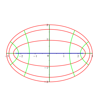
Figure 1. Coordinate lines of ellipsoidal coordinates

From (2.7), (2.8), (2.9) we find the metric tensor in terms of the coordinates $s,t$

(2.10) $$g_{1} = (c^{2}\operatorname{cn}^{2}(s,k^{\prime})+b^{2}\operatorname{sn}^{2}(s,k^{\prime}))(\operatorname{dn}^{2}(s,k^{\prime})-k^{2}\operatorname{sn}^{2}(t,k)),$$

(2.11) $$g_{2} = (a^{2}\operatorname{cn}^{2}(t,k)+b^{2}\operatorname{sn}^{2}(t,k))(\operatorname{dn}^{2}(s,k^{\prime})-k^{2}\operatorname{sn}^{2}(t,k)),$$

(2.12) $$g_{12} = 0.$$

3. The Laplace-Beltrami operator

In terms of the coordinates $\mu,\nu$ the Laplace-Beltrami operator $\Delta_{\mathcal{E}}$ on the ellipsoid $\mathcal{E}$ is given by

$$\Delta_{\mathcal{E}}u=(g_{1}g_{2})^{-1/2}\left(\frac{\partial}{\partial\mu}\left(g_{2}^{1/2}g_{1}^{-1/2}\frac{\partial\mu}{\partial\mu}\right)+\frac{\partial}{\partial\nu}\left(g_{1}^{1/2}g_{2}^{-1/2}\frac{\partial\nu}{\partial\nu}\right)\right)\\ =\frac{1}{\mu-\nu}\left(\frac{1}{F(\mu)^{1/2}}\frac{\partial}{\partial\mu}\left(\frac{1}{F(\mu)^{1/2}}\frac{\partial u}{\partial\mu}\right)+\frac{1}{(-F(\nu))^{1/2}}\frac{\partial}{\partial\nu}\left(\frac{1}{(-F(\nu))^{1/2}}\frac{\partial u}{\partial\nu}\right)\right).$$

In the eigenvalue equation $-\Delta_{\mathcal{E}}u=\lambda u$ we can separate variables as follows. If $v(\mu)$ is a solution of the differential equation

(3.1) $$\frac{d}{d\mu}\left(\frac{1}{F(\mu)^{1/2}}\frac{dv}{d\mu}\right)+F(\mu)^{1/2}(\lambda\mu-hk^{-2})v=0,\quad 1<\mu<k^{-2},$$

and $w(\nu)$ is a solution of the differential equation

(3.2) $$\frac{d}{d\nu}\left(\frac{1}{(-F(\nu))^{1/2}}\frac{dw}{d\nu}\right)-(-F(\nu))^{1/2}(\lambda\nu-hk^{-2})w=0,\quad 0<\nu<1,$$

then $u(\mu,\nu)=v(\mu)w(\nu)$ is a solution of $-\Delta_{\mathcal{E}}u=\lambda u$ on $\mathcal{E}_{+}$. In these equations $h$ denotes the separation parameter.

Equation (3.1) can be written in the form

(3.3) $$\frac{d^{2}v}{d\mu^{2}}+\frac{1}{2}\left(\frac{1}{\mu}+\frac{1}{\mu-1}+\frac{1}{\mu-k^{-2}}-\frac{1}{\mu-d}\right)\frac{dv}{d\mu}+(\lambda\mu-hk^{-2})F(\mu)v=0,$$

where

$$d:=\frac{a^{2}}{a^{2}-b^{2}}>k^{-2}.$$

Equation (3.2) can be written in exactly the same form with $\nu$ replacing $\mu$ and $w$ replacing $v$. Therefore, the differential equations (3.1), (3.2) are actually the same equation but they are considered on different intervals. It is interesting to note that equation (3.3) has five singularities at $0,1,k^{-2},d$ and $\infty$. The first four are regular singularities [13, Ch. 5, §4] with indices $\{0,\frac{1}{2}\}$, $\{0,\frac{1}{2}\}$, $\{0,\frac{1}{2}\}$, $\{0,\frac{3}{2}\}$ respectively but $\infty$ is an irregular singularity unless $\lambda=0$. Equation (3.3) can be considered as an extension of the Lamé equation (1.2) in its algebraic form [14, 29.2.2]. The Lamé equation has only four singularities at $0,1,k^{-2},\infty$ and all of them are regular. The additional singularity $d$ appears in connection with the Laplace-Beltrami operator on the ellipsoid and makes the differential equation more difficult to treat.

Since the singularities $0,1,k^{-2}$ are regular and each has index $0$, equation (3.3) admits nontrivial Fuchs-Frobenius power series solutions in powers of $\mu$, $\mu-1$ and $\mu-k^{-2}$. Usually, these solutions are not connected by analytic continuation. We are interested in the exceptional case that all three solutions are connected.

Lemma 2.

Let the parameters $\lambda$, $h$ be such that differential equation (3.3) admits a nontrivial analytic solution $f(\mu)$ on an open region $D$ containing the interval $[0,k^{-2}]$. Then the function $u$ on $\mathcal{E}$ defined by $f(\mu)f(\nu)$ is an analytic function on $\mathcal{E}$ with parity $(0,0,0)$ and it is an eigenfunction of $-\Delta_{\mathcal{E}}$ corresponding to the eigenvalue $\lambda$.

Proof.

It follows from Lemma 1 that $u$ is analytic on $\mathcal{E}$. By our derivation, we know that $u$ solves $-\Delta_{\mathcal{E}}u=\lambda u$ on $\mathcal{E}_{+}$. Both $u$ and $\Delta_{\mathcal{E}}u$ have the same parity $(0,0,0)$ so $-\Delta_{\mathcal{E}}u=\lambda u$ holds on $\mathcal{E}$. ∎

Note that in the situation of Lemma 2 the region $D$ can be taken as the entire complex plane with the branch cut $[d,\infty)$ removed.

4. A two-parameter Sturm-Liouville problem

Our goal is to prove existence of pairs $\lambda,h$ as indicated in Lemma 2, and to show that the corresponding $\lambda$’s comprise all eigenvalues of $-\Delta_{\mathcal{E}}$ having eigenfunction with parity $(0,0,0)$. To that purpose we prefer to use the transcendental ellipsoidal coordinates $s,t$ because then we arrive at a regular two-parameter Sturm-Liouville system. If we use the coordinates $\mu,\nu$ then our Sturm-Liouville problems have singular endpoints which makes theoretical and numerical work more difficult.

We set $\mu=k^{-2}\operatorname{dn}^{2}(s,k^{\prime})$ and $\nu=\operatorname{sn}^{2}(t,k)$ in (3.3), and, after some computations, we obtain

(4.1) $$\frac{d}{ds}\left(\frac{1}{p(s)}\frac{dv}{ds}\right)+p(s)(-h+\lambda\operatorname{dn}^{2}(s,k^{\prime}))v=0,$$

(4.2) $$\frac{d}{dt}\left(\frac{1}{q(t)}\frac{dw}{dt}\right)+q(t)(h-\lambda k^{2}\operatorname{sn}^{2}(t,k))w=0,$$

where

(4.3) $$p(s) := (c^{2}\operatorname{cn}^{2}(s,k^{\prime})+b^{2}\operatorname{sn}^{2}(s,k^{\prime}))^{1/2},$$

(4.4) $$q(t) := (a^{2}\operatorname{cn}^{2}(t,k)+b^{2}\operatorname{sn}^{2}(t,k))^{1/2}.$$

When we substitute $t=K+iK^{\prime}-is$, $s\in\mathbb{R}$, and use the identities

$$k\operatorname{sn}(t,k)=\operatorname{dn}(s,k^{\prime}),\,k\operatorname{cn}(t,k)=-ik^{\prime}\operatorname{cn}(s,k^{\prime}),\,\operatorname{dn}(t,k)=k^{\prime}\operatorname{sn}(s,k^{\prime}),$$

we find that $p(s)=q(t)$ and equation (4.1) transforms to (4.2). So we may say that (4.1), (4.2) are the same differential equations but considered on different intervals in the complex plane. Note also that equation (4.1) can be obtained from (4.2) by interchanging $a$ with $c$ (which automatically interchanges $k$ with $k^{\prime}$) and replacing $h$ by $\lambda-h$. If we put $q(t)=1$ then (4.2) is the Lamé equation (1.2) in its standard form, so (4.2) can be seen as a generalization of the Lamé equation. We add the Neumann boundary conditions

(4.5) $$v^{\prime}(0) = v^{\prime}(K^{\prime})=0,$$

(4.6) $$w^{\prime}(0) = w^{\prime}(K)=0.$$

They correspond to the conditions that $v$ as a function of $\mu$ is a Fuchs-Frobenius solution of (3.3) at $\mu=1$ and $\mu=k^{-2}$ belonging to the indices $0$, and $w$ as a function of $\nu$ is a Fuchs-Frobenius solution of (3.3) at $\nu=0$ and $\nu=1$ belonging to the indices $0$.

For every fixed real $\lambda$, equation (4.1) subject to boundary conditions (4.5) poses a regular Sturm-Liouville problem [17, §27] with spectral parameter $-h$. Similarly, for every fixed real $\lambda$, (4.2) subject to boundary conditions (4.6) poses a regular Sturm-Liouville problem with spectral parameter $h$. If we combine these problems we obtain a regular two-parameter Sturm-Liouville problem [2]. A pair $\lambda,h$ is called an eigenvalue of this problem if there exist a nontrivial solution $v(s)$, $0\leq s\leq K^{\prime}$, of (4.1), (4.5) and a nontrivial solution $w(t)$, $0\leq t\leq K$, of (4.2), (4.6). If $\lambda,h$ is an eigenvalue of this two-parameter Sturm-Liouville problem, then Lemma 2 shows that $\lambda$ is an eigenvalue of $-\Delta_{\mathcal{E}}$ having an eigenfunction of parity $(0,0,0)$.

If $v(s)$ is a solution of equation (4.1) then $v(s+2K^{\prime})$ and $v(-s)$ are also solutions. Therefore, a solution $v(s)$ of (4.1) satisfies the boundary conditions (4.5) if and only if it is even and has period $2K^{\prime}$. A similar remark applies to equation (4.2). Taking into account the substitution $t=K+iK^{\prime}-is$, we see that $\lambda,h$ is an eigenvalue if and only if equation (4.2) admits a nontrivial analytic solution $w(t)$ defined on the union $S_{1}\cup S_{2}$ of two strips

$$S_{1}:=\{t\in\mathbb{C}:|\Im t|<\delta\},\quad S_{2}=\{t\in\mathbb{C}:|\Re t-K|<\delta\}$$

for some sufficiently small positive $\delta$ such that $w(t)$ has period $2K$ on $S_{1}$, period $2iK^{\prime}$ on $S_{2}$ and, in addition, is even with respect to $K$, that is, $w(t)=w(2K-t)$. So the eigenvalue problem consists in finding doubly-periodic solutions of (4.2).

For every $\lambda\in\mathbb{R}$, the eigenvalues of the regular Sturm-Liouville problem (4.2), (4.6) form an increasing sequence

$$h_{0}(\lambda)<h_{1}(\lambda)<h_{2}(\lambda)<\dots$$

which diverges to $\infty$. The subscript $n$ of $h_{n}(\lambda)$ denotes the number of zeros of a corresponding eigenfunction $w_{n}(t)$ in the interval $(0,K)$. The graph of the eigenvalue functions $h_{n}(\lambda)$ are called eigencurves [2, Chapter 6]. Similarly, equation (4.1) (with $h$ replaced by $H$) subject to conditions (4.5) generates eigenvalue functions

$$H_{0}(\lambda)>H_{1}(\lambda)>H_{2}(\lambda)>\dots$$

where the subscript $m$ of $H_{m}(\lambda)$ denotes the number of zeros of an eigenfunction $v_{m}(s)$ in the interval $(0,K^{\prime})$. The eigenvalues $\lambda,h$ of the two-parameter eigenvalue problem are exactly the intersection points of eigencurves $H_{m}(\lambda)$ and $h_{n}(\lambda)$, $m,n\in\mathbb{N}_{0}$. A few eigencurves are shown in Figure 2 in Section 8.

We mention some properties of eigencurves proved in [4]. We cannot directly apply the results from [4] to (4.1), (4.2) because in [4] it is assumed that the factor of $h$ is identically one. However, we can transform this factor to $1$ by a substitution of the independent variable. For example, in (4.2) we introduce a new variable $\tau$ by setting

$$\frac{d\tau}{dt}=q(t).$$

Then (4.2) becomes

(4.7) $$-\frac{d^{2}w}{d\tau^{2}}=(h+\lambda r(\tau))w,\quad r(\tau)=-k^{2}\operatorname{sn}^{2}(t,k).$$

Equation (4.7) has the form treated in [4]. Actually, equation (4.7) looks simpler than (4.2) but, unfortunately, we do not have an explicit formula for $r(\tau)$ in terms of $\tau$.

By [4, Theorem 2.1], $H_{m}(\lambda)$ and $h_{n}(\lambda)$ are analytic functions of $\lambda$. Their first derivatives [4, (2.5)] are given by

$$H_{m}^{\prime}(\lambda)=\frac{\int_{0}^{K^{\prime}}p(s)\operatorname{dn}^{2}(s,k^{\prime})v_{m}(s)^{2}\,ds}{\int_{0}^{K^{\prime}}p(s)v_{m}(s)^{2}\,ds},$$

$$h_{n}^{\prime}(\lambda)=\frac{\int_{0}^{K}q(t)k^{2}\operatorname{sn}^{2}(t,k)w_{n}(t)^{2}\,dt}{\int_{0}^{K}q(t)w_{n}(t)^{2}\,dt}.$$

It follows from $k^{2}<\operatorname{dn}^{2}(s,k^{\prime})<1$ on $(0,K^{\prime})$ and $0<\operatorname{sn}^{2}(t,k)<1$ on $(0,K)$ that

(4.8) $$0<h_{n}^{\prime}(\lambda)<k^{2}<H_{m}^{\prime}(\lambda)<1\quad\text{for all $\lambda\in\mathbb{R}$}.$$

Regarding the asymptotic behavior of the eigencurves as $\lambda\to\infty$ we have from [4, Theorem 2.2]

(4.9) $$\lim_{\lambda\to\infty}\frac{H_{m}(\lambda)}{\lambda}=1,\quad\lim_{\lambda\to\infty}\frac{h_{n}(\lambda)}{\lambda}=0.$$

If $\lambda=0$ then we can solve (4.1) and (4.2) explicitly. The solution of (4.1) with $\lambda=0$ and initial conditions $v(0)=1$, $v^{\prime}(0)=0$ is

$$v(s)=\cos\left((-h)^{1/2}\int_{0}^{s}p(\sigma)\,d\sigma\right).$$

Using this formula and a similar one for (4.2), we obtain

(4.10) $$H_{m}(0) = -m^{2}\pi^{2}\left(\int_{0}^{K^{\prime}}p(s)\,ds\right)^{-2}\quad\text{for $m\in\mathbb{N}_{0}$,}$$

(4.11) $$h_{n}(0) = n^{2}\pi^{2}\left(\int_{0}^{K}q(t)\,dt\right)^{-2}\quad\text{for $n\in\mathbb{N}_{0}$.}$$

Theorem 3.

For every pair $m,n\in\mathbb{N}_{0}$, there is exactly one intersection point $(\lambda_{m,n},h_{m,n})$ of the eigencurves $H_{m}(\lambda)$ and $h_{n}(\lambda)$. We have $\lambda_{0,0}=h_{0,0}=0$ and $\lambda_{m,n}>0$, $h_{m,n}>0$ for all $(m,n)\neq(0,0)$.

Proof.

Let $m,n\in\mathbb{N}_{0}$. It follows from (4.8) that there is at most one $\lambda$ such that $H_{m}(\lambda)=h_{n}(\lambda)$. By (4.10), (4.11) we know that $H_{m}(0)\leq 0\leq h_{n}(0)$. Therefore, by (4.9), there exists $\lambda$ such that $H_{m}(\lambda)=h_{n}(\lambda)$. If $m=n=0$ then $\lambda=0$ and $H_{0}(0)=h_{0}(0)=0$. Otherwise, $\lambda>0$ and $h_{n}(\lambda)>0$. ∎

Our two-parameter Sturm-Liouville problem is right-definite, that is,

$$D(s,t):=\begin{vmatrix}p(s)\operatorname{dn}^{2}(s,k^{\prime})&-p(s)\\ -q(t)k^{2}\operatorname{sn}^{2}(t,k)&q(t)\end{vmatrix}=p(s)q(t)(\operatorname{dn}^{2}(s,k^{\prime})-k^{2}\operatorname{sn}^{2}(t,k))>0$$

for all $s\in[0,K^{\prime}]$ and $t\in[0,K]$ with the exception of $s=K^{\prime}$, $t=K$, where the determinant vanishes. It is well known [2, Theorem 5.5.1] that right-definiteness implies the existence and uniqueness of the intersection points $(\lambda_{m,n},h_{m,n})$ of eigencurves as stated in Theorem 3.

Let $v_{m,n}(s)$ and $w_{m,n}(t)$ denote real-valued eigenfunctions satisfying (4.1), (4.2), (4.5), (4.6) for $\lambda=\lambda_{m,n}$ and $h=h_{m,n}$. It is easy to prove [2, Section 3.5] that the system of products

$$u_{m,n}(s,t):=v_{m,n}(s)w_{m,n}(t),\quad m,n\in\mathbb{N}_{0},$$

is orthogonal with respect to the inner product

$$\langle f,g\rangle=\int_{0}^{K}\int_{0}^{K^{\prime}}D(s,t)f(s,t)\overline{g(s,t)}\,ds\,dt.$$

We notice that

$$D(s,t)=g_{1}^{1/2}g_{2}^{1/2}$$

if $g_{1}$ and $g_{2}$ are expressed in ellipsoidal coordinates $s,t$ according to (2.10), (2.11). This shows that the eigenfunctions $u_{m,n}$ of $-\Delta_{\mathcal{E}}$ are orthogonal in $L^{2}(\mathcal{E})$ because the surface measure of $\mathcal{E}$ has the form $dS=g_{1}^{1/2}g_{2}^{1/2}\,ds\,dt$. We normalize the functions $u_{m,n}$ so that they have norm $1$ in $L^{2}(\mathcal{E})$.

According to [15, Theorem 6.8.3] we have the following completeness result.

Theorem 4.

The double sequence $u_{m,n}$, $m,n\in\mathbb{N}_{0}$, forms an orthonormal basis for the subspace of $L^{2}(\mathcal{E})$ consisting of functions with parity $(0,0,0)$.

Theorem 5.

Every number $\lambda_{m,n}$, $m,n\in\mathbb{N}_{0}$, is an eigenvalue of the Laplace-Beltrami operator $-\Delta_{\mathcal{E}}$ with corresponding eigenfunction $u_{m,n}$ of parity $(0,0,0)$. Every eigenvalue of $-\Delta_{\mathcal{E}}$ with an eigenfunction of parity $(0,0,0)$ is equal to one of the $\lambda_{m,n}$

Proof.

We already mentioned that each $\lambda_{m,n}$ is an eigenvalue of $-\Delta_{\mathcal{E}}$ with eigenfunction $u_{m,n}$. If $-\Delta_{\mathcal{E}}$ had an eigenvalue $\lambda$ with an eigenfunction $u$ of parity $(0,0,0)$ such that $\lambda$ is different from any $\lambda_{m,n}$ then $u$ would be orthogonal to each $u_{m,n}$, and this is impossible by Theorem 4. ∎

5. Eigenfunctions of other parities

Let $\kappa_{1},\kappa_{2},\kappa_{3}\in\{0,1\}$. We say that a function $f:\mathcal{E}\to\mathbb{C}$ has parity $(\kappa_{1},\kappa_{2},\kappa_{3})$ if

$$f(x,y,z)=(-1)^{\kappa_{1}}f(-x,y,z)=(-1)^{\kappa_{2}}f(x,-y,z)=(-1)^{\kappa_{3}}f(x,y,-z).$$

Since the Laplace-Beltrami operator $\Delta_{\mathcal{E}}$ leaves the parity of a function invariant, it is sufficient to look for eigenvalues of $-\Delta_{\mathcal{E}}$ with eigenfunctions of a given parity. This splits the eigenvalue problem for $-\Delta_{\mathcal{E}}$ into eight subproblems. We already proved some results on the eigenvalues of $-\Delta_{\mathcal{E}}$ with eigenfunctions of parity $(0,0,0)$. We now mention analogous results for the other seven parities.

The differential equations (3.3), (4.1) and (4.2) stay the same in all eight cases only the boundary conditions (4.5), (4.6) change. We need a nontrivial solution of (3.3) of the form

$$\mu^{\kappa_{1}/2}(\mu-1)^{\kappa_{2}/2}(\mu-k^{-2})^{\kappa_{3}/2}g(\mu),$$

where $g$ is an analytic function on an open region containing the interval $[0,k^{-2}]$, that is, a nontrivial solution of (3.3) which is simultaneously a Fuchs-Frobenius solution at the points $0,1,k^{-2}$ belonging to the indices $\kappa_{1}/2,\kappa_{2}/2,\kappa_{3}/2$, respectively. These conditions translate to boundary conditions for (4.1), (4.2) as follows:

(5.1) $$v^{\prime}(0)=0\text{ if $\kappa_{3}=0$}, v(0)=0\text{ if $\kappa_{3}=1$},$$

(5.2) $$v^{\prime}(K^{\prime})=w^{\prime}(K)=0\text{ if $\kappa_{2}=0$}, v(K^{\prime})=w(K)=0\text{ if $\kappa_{2}=1$},$$

(5.3) $$w^{\prime}(0)=0\text{ if $\kappa_{1}=0$}, w(0)=0\text{ if $\kappa_{1}=1$}.$$

For each $\kappa=(\kappa_{1},\kappa_{2},\kappa_{3})\in\{0,1\}^{3}$ we obtain a regular two-parameter Sturm-Liouville problem for the differential equations (4.1), (4.2) subject to boundary conditions (5.1), (5.2), (5.2). We denote the corresponding eigenvalue functions by $H_{m,\kappa}(\lambda;a,b,c)$ and $h_{n,\kappa}(\lambda;a,b,c)$. The solution $\lambda$ of $H_{m,\kappa}(\lambda;a,b,c)=h_{n,\kappa}(\lambda;a,b,c)$ we denote by $\lambda_{m,n,\kappa}(a,b,c)$. This number $\lambda_{m,n,\kappa}(a,b,c)$ is an eigenvalue of the Laplace-Beltrami operator $-\Delta_{\mathcal{E}}$, and every eigenvalue of $-\Delta_{\mathcal{E}}$ is of this form. We recall that $a,b,c$ denote the semi-axes of the ellipsoid $\mathcal{E}$, $\kappa$ is the parity of a corresponding eigenfunction $u_{m}(s)w_{n}(t)$ when considered as a function on $\mathcal{E}$, $m$ is the number of zeros of $v_{m}$ in $(0,K^{\prime})$, and $n$ is the number of zeros of $w_{n}$ in $(0,K)$.

For each parity we get analogues of Theorems 3, 4, 5. In Theorem 5 we have $\lambda_{m,n,\kappa}(a,b,c)>0$ except in the trivial case $\lambda_{0,0,(0,0,0)}(a,b,c)=0$.

6. The Laplace-Beltrami operator on the sphere

It is of interest to compare the two-parameter Sturm-Liouville problem (4.1), (4.2) subject to boundary conditions (5.1), (5.2), (5.3) with a well-known simpler problem that we obtain when treating the Laplace-Beltrami operator $\Delta_{\mathcal{S}}$ on the sphere

$$\mathcal{S}=\{(x,y,z):x^{2}+y^{2}+z^{2}=1\}.$$

We introduce sphero-conal coordinates $\mu,\nu$ on $\mathcal{S}$ by (2.1), (2.2), (2.3) with $a=b=c=1$. It is important to note that in case of the ellipsoid $\mathcal{E}$ the parameter $k$ is defined by (2.4) whereas $k\in(0,1)$ is arbitrary in case of the sphere. We then proceed as we did for the Laplace-Beltrami operator on the ellipsoid. The differential equation (3.3) becomes the Lamé equation [14, 29.2.2] in its algebraic form, and (4.2) becomes the Lamé equation in its Jacobian form. We obtain a two-parameter Sturm-Liouville problem consisting of differential equations (4.1), (4.2) with $p(s)=q(t)=1$ subject to boundary conditions (5.1), (5.2), (5.3). We will denote the corresponding eigenvalue functions by $H_{m,\kappa}(\lambda,k)$, $h_{n,\kappa}(\lambda,k)$ and the solution $\lambda$ of $H_{m,\kappa}(\lambda,k)=h_{n,\kappa}(\lambda,k)$ by $\Lambda_{m,n,\kappa}$ (which is independent of $k$). These numbers $\Lambda_{m,n,\kappa}$ are eigenvalues of $-\Delta_{\mathcal{S}}$ and they are given by

(6.1) $$\Lambda_{m,n,\kappa}=(2m+2n+|\kappa|)(2m+2n+|\kappa|+1),\quad|\kappa|:=\kappa_{1}+\kappa_{2}+\kappa_{3}.$$

An eigenfunction of $-\Delta_{\mathcal{S}}$ corresponding to the eigenvalue $\ell(\ell+1)$ is given by the sphero-conal harmonic

(6.2) $$U_{m,n,\kappa}(s,t)=V_{m,n,\kappa}(s)W_{m,n,\kappa}(t),$$

where $2m+2n+|\kappa|=\ell$, $W_{m,n,\kappa}(t)$ is a Lamé polynomial and

$$V_{m,n,\kappa}(s)=W_{m,n,\kappa}(K+iK^{\prime}-is).$$

The Lamé polynomial $w(t)=W_{m,n,\kappa}(t)$ is a solution of the Lamé equation

$$w^{\prime\prime}+\left(h_{n,\kappa}(\ell(\ell+1),k)-\ell(\ell+1)k^{2}\operatorname{sn}^{2}(t,k)\right)w=0$$

of the form

$$w(t)=\operatorname{sn}^{\kappa_{1}}(t,k)\operatorname{cn}^{\kappa_{2}}(t,k)\operatorname{dn}^{\kappa_{3}}(t,k)P(\operatorname{sn}^{2}(t,k)),$$

where $P$ is a polynomial of degree $m+n$. Moreover, $V_{m,n,\kappa}(s)$ has $m$ zeros in $(0,K^{\prime})$ and $W_{m,n,\kappa}(t)$ has $n$ zeros in $(0,K)$. For more details on Lamé polynomials we refer to Arscott [1, Chapter IX]. Arscott distinguishes eight species of Lamé polynomials which correspond to the eight parities $\kappa\in\{0,1\}^{3}$ in our notation.

7. The Prüfer transformation

We introduce the Prüfer radius $r(t)>0$ and the Prüfer angle $\theta(t)$ [17, §27.IV] for system (4.2), (4.6) by setting

$$w(t)=r(t)\sin\theta(t),\quad\frac{w^{\prime}(t)}{q(t)}=r(t)\cos\theta(t).$$

Then $\theta(t)$ satisfies the first-order differential equation

(7.1) $$\frac{d\theta}{dt}=q(t)\left(\cos^{2}\theta+(h-\lambda k^{2}\operatorname{sn}^{2}(t,k))\sin^{2}\theta\right)$$

with initial condition

(7.2) $$\theta(0)=\tfrac{1}{2}(1-\kappa_{1})\pi.$$

The pair $(\lambda,h)$ lies on the $n$th eigencurve if

(7.3) $$\theta(K)=\tfrac{1}{2}(1+\kappa_{2})\pi+n\pi.$$

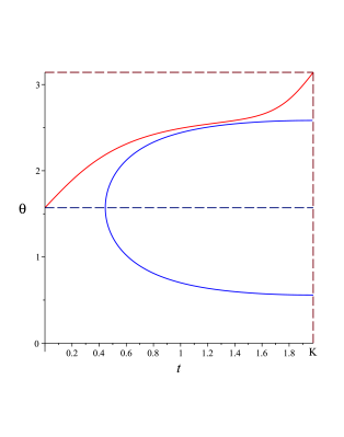
Figure 2. The Prüfer angle $\theta(t)$ (in red) and the curve on which the right-hand side of (7.1) vanishes (in blue).

Consider the example $a=3$, $b=2$, $c=1$, $\kappa_{1}=0$, $\kappa_{2}=1$, $\lambda=5$ and $n=0$. Then $h_{n,\kappa}(\lambda)=0.558216\dots$ and the graph of $\theta(t)$ is shown in Figure 2.

Lemma 6.

If $\kappa_{2}=1$, $\lambda>0$ and $n\in\mathbb{N}_{0}$, then every solution $\theta(t)$ of (7.1), (7.2) and (7.3) satisfies $\theta^{\prime}(t)>0$ for $t\in[0,K]$.

Proof.

We know that $h>0$. If $h-\lambda k^{2}>0$ then $h-\lambda k^{2}\operatorname{sn}^{2}(t,k)>0$ for all $t\in[0,K]$ and the statement of the lemma follows immediately from (7.1). Now suppose that $h-\lambda k^{2}\leq 0$. Then the region

$$R:=\{(t,\theta)\in[0,K]\times\mathbb{R}:\cos^{2}\theta+(h-\lambda k^{2}\operatorname{sn}^{2}(t,k))\sin^{2}\theta<0\}$$

is given by

$$R=\{(t,\theta):G(\theta)<t\leq K\},$$

where

$$G(\theta)={\rm arcsn}\left(\frac{h+\cot^{2}\theta}{\lambda k^{2}}\right)^{1/2}.$$

This function is only defined for $\theta$ with $h+\cot^{2}\theta\leq\lambda k^{2}$. In Figure 2 $R$ is the region to the right of the blue curve. Our goal is to show that the graph of $\theta(t)$ cannot enter the region $R$.

If the point $(t_{1},\theta(t_{1}))$ lies on the boundary of $R$ then $\theta^{\prime}(t_{1})=0$ and so $(t,\theta(t))$ is outside the closure $\bar{R}$ of $R$ for $t<t_{1}$ close to $t_{1}$. Therefore, once the graph of $\theta(t)$ enters $\bar{R}$ it must stay in $\bar{R}$. Since all points $(K,\ell\pi)$, $\ell\in\mathbb{Z}$, lie outside of $\bar{R}$, and $\kappa_{2}=1$, the graph of $\theta(t)$ stays outside of $\bar{R}$ and so $\theta^{\prime}(t)>0$ for all $t\in[0,K]$. ∎

If $\kappa_{2}=0$ then Lemma 6 is not always true. For example, if $\kappa_{1}=\kappa_{2}=0$ and $n=0$, then $\theta(0)=\theta(K)=\tfrac{1}{2}\pi$, so $\theta^{\prime}(t)$ cannot be positive for all $t\in[0,K]$. If $\theta^{\prime}(t)$ is not positive throughout the interval $[0,K]$ then arguing as in the proof of Lemma 6 one can show that there is $t_{0}\in(0,K]$ such that $\theta^{\prime}(t_{0})=0$, $\theta^{\prime}(t)>0$ for $t\in[0,t_{0})$ and $\theta^{\prime}(t)<0$ for $t\in(t_{0},K]$.

Theorem 7.

For all $m,n\in\mathbb{N}_{0}$ and all parities $\kappa=(\kappa_{1},\kappa_{2},\kappa_{3})$ with $\kappa_{2}=1$ we have

(7.4) $$a^{-2}\Lambda_{m,n,\kappa}<\lambda_{m,n,\kappa}(a,b,c)<c^{-2}\Lambda_{m,n,\kappa},$$

where $\Lambda_{m,n,\kappa}$ is given by (6.1). If $\kappa_{2}=0$ then

(7.5) $$\lambda_{m,n,\kappa}(a,b,c)<c^{-2}\Lambda_{m,n,\hat{\kappa}},$$

where $\hat{\kappa}=(\kappa_{1},1,\kappa_{2})$. If $\kappa_{2}=0$ and $m,n\geq 1$, then

(7.6) $$a^{-2}\Lambda_{m-1,n-1,\hat{\kappa}}<\lambda_{m,n,\kappa}(a,b,c).$$

Proof.

Since $\lambda_{m,n,\kappa}(ra,rb,rc)=r^{-2}\lambda_{m,n,\kappa}(a,b,c)$ it is sufficient to assume that $c=1$ in the proof of the second inequality in (7.4). Then the function $q(t)$ defined by (4.4) satisfies $q(t)>1$. Let $\psi(t)$ be the solution of the differential equation

(7.7) $$\frac{d\psi}{dt}=f(t,\psi):=\cos^{2}\psi+(h-\lambda k^{2}\operatorname{sn}^{2}(t,k))\sin^{2}\psi$$

determined by the initial condition $\psi(0)=\frac{1}{2}(1-\kappa_{1})\pi$. Then Lemma 6 gives

$$\theta^{\prime}(t)-f(t,\theta(t))=\theta^{\prime}(t)(1-q(t)^{-1})>0=\psi^{\prime}(t)-f(t,\psi(t)).$$

We also have $\psi(0)=\theta(0)$ and $\psi^{\prime}(0)<\theta^{\prime}(0)$. Now the comparison theorem [18, II.9.III] yields $\psi(t)<\theta(t)$ for $0<t\leq K$. Using this inequality for $t=K$ we obtain from (7.3) that

$$h_{n,\kappa}(\lambda;a,b,c)<h_{n,\kappa}(\lambda,k).$$

Since $p(s)>1$ for $0<s\leq K^{\prime}$, we can show in a similar way that

$$H_{m,\kappa}(\lambda;a,b,c)>H_{m,\kappa}(\lambda,k).$$

Let $\lambda_{0}=\lambda_{m,n,\kappa}(a,b,c)$. Then

$$H_{m,\kappa}(\lambda_{0},k)<H_{m,\kappa}(\lambda_{0};a,b,c)=h_{n,\kappa}(\lambda_{0};a,b,c)<h_{n,\kappa}(\lambda_{0},k).$$

Therefore, if we set $g(\lambda)=H_{m,\kappa}(\lambda,k)-h_{n,k}(\lambda,k)$, then $g(\lambda_{0})<0$. Now $g(\Lambda_{m,n,\kappa})=0$ and $g(\lambda)$ is an increasing function so $\lambda_{0}<\Lambda_{m,n,\kappa}$ completing the proof of the second inequality in (7.4). The first inequality is proved in a very similar way.

To prove (7.5), we assume $\kappa_{2}=0$ and $c=1$. Then we have

$$H_{m,\kappa}(\lambda;a,b,c)>H_{m,\hat{\kappa}}(\lambda;a,b,c),\quad h_{n,\kappa}(\lambda;a,b,c)<h_{n,\hat{\kappa}}(\lambda;a,b,c)$$

so $\lambda_{m,n,\kappa}(a,b,c)<\lambda_{m,n,\hat{\kappa}}(a,b,c)$. Now (7.5) follows from (7.4) applied to $\hat{\kappa}$ in place of $\kappa$.

Inequality (7.6) is proved in a similar way. ∎

8. Approximation by matrix eigenvalue problems

The eigenvalue functions $h_{n}(\lambda)$ for equation (4.2) can be computed using the Prüfer angle by the SLEIGN2 code [3]. However, we present another method which approximates the eigenvalues $h_{n}(\lambda)$ by eigenvalues of finite matrices. We transform the differential equation (4.2) into trigonometric form and then expand eigenfunctions in Fourier series. This method was used by Ince [10] in order to compute eigenvalues of the Lamé equation (1.2).

Following Erdélyi [6, (4), page 56] we substitute

$$\tau=\tfrac{1}{2}\pi-\operatorname{am}(t,k)$$

in (4.2) where $\operatorname{am}$ denotes the Jacobian amplitude function [14, §22.16.(i)]. We multiply (4.2) by $q(t)^{3}$ and use

$$\frac{d\tau}{dt}=-\operatorname{dn}(t,k),\quad\operatorname{cn}(t,k)=\sin\tau,\quad\operatorname{sn}(t,k)=\cos\tau.$$

Then we obtain

(8.1) $$Dw+\lambda Cw=hBw$$

where $D$ is the differential operator

(8.2) $$Dw:=-(a^{2}\sin^{2}\tau+b^{2}\cos^{2}\tau)(1-k^{2}\cos^{2}\tau)\frac{d^{2}w}{d\tau^{2}}-c^{2}k^{2}\cos\tau\sin\tau\frac{dw}{d\tau}$$

and $C,B$ are multiplication operators

$$Cw := k^{2}\cos^{2}\tau(a^{2}\sin^{2}\tau+b^{2}\cos^{2}\tau)^{2}w,$$

$$Bw := (a^{2}\sin^{2}\tau+b^{2}\cos^{2}\tau)^{2}w.$$

The boundary conditions corresponding to (4.6) are

(8.3) $$w^{\prime}(0)=w^{\prime}(\tfrac{1}{2}\pi)=0,\quad^{\prime}=\frac{d}{d\tau}.$$

We compute the matrix representation of $D$ in the trigonometric basis $\cos(2n\tau)$, $n\in\mathbb{N}_{0}$. Using

$$(a^{2}\sin^{2}\tau+b^{2}\cos^{2}\tau)(1-k^{2}\cos^{2}\tau)=\\ \tfrac{1}{2}(a^{2}+b^{2})-\tfrac{1}{8}k^{2}(a^{2}+3b^{2})+\tfrac{1}{2}(b^{2}-a^{2}-b^{2}k^{2})\cos(2\tau)+\tfrac{1}{8}k^{2}(a^{2}-b^{2})\cos(4\tau)$$

we obtain

(8.4) $$D\cos (2n\tau)=n^{2}\left(2(a^{2}+b^{2})-\tfrac{1}{2}k^{2}(a^{2}+3b^{2})\right)\cos(2n\tau)$$

$$+n^{2}(b^{2}-a^{2}-b^{2}k^{2})(\cos((2n-2)\tau)+\cos((2n+2)\tau))$$

$$+\tfrac{1}{4}n^{2}k^{2}(a^{2}-b^{2})(\cos((2n-4)\tau)+\cos((2n+4)\tau))$$

$$+\tfrac{1}{2}nc^{2}k^{2}(\cos((2n-2)\tau)-\cos((2n+2)\tau)).$$

Similarly,

$$(a^{2}\sin^{2}\tau+b^{2}\cos^{2}\tau)^{2}\cos^{2}\tau=\tfrac{1}{16}(a^{4}+2a^{2}b^{2}+5b^{4})\\ +\tfrac{1}{32}(15b^{4}+2a^{2}b^{2}-a^{4})\cos(2\tau)+\tfrac{1}{16}(b^{2}-a^{2})(a^{2}+3b^{2})\cos(4\tau)+\tfrac{1}{32}(a^{2}-b^{2})^{2}\cos(6\tau).$$

gives

(8.5) $$C\cos (2n\tau)=\tfrac{1}{16}k^{2}(a^{4}+2a^{2}b^{2}+5b^{4})\cos(2n\tau)$$

$$+\tfrac{1}{64}k^{2}(15b^{4}+2a^{2}b^{2}-a^{4})(\cos((2n-2)\tau)+\cos((2n+2)\tau))$$

$$+\tfrac{1}{32}k^{2}(b^{2}-a^{2})(a^{2}+3b^{2})(\cos((2n-4)\tau)+\cos((2n+4)\tau))$$

$$+\tfrac{1}{64}k^{2}(a^{2}-b^{2})^{2}(\cos((2n-6)\tau)+\cos((2n+6)\tau)).$$

Finally,

$$(a^{2}\sin^{2}\tau+b^{2}\cos^{2}\tau)^{2}=\\ \tfrac{1}{8}(3a^{4}+2a^{2}b^{2}+3b^{4})+\tfrac{1}{2}(b^{4}-a^{4})\cos(2\tau)+3a^{4})+\tfrac{1}{8}(a^{2}-b^{2})^{2}\cos(4\tau)$$

gives

(8.6) $$B\cos (2n\tau)=\tfrac{1}{8}(3a^{4}+2a^{2}b^{2}+3b^{4})\cos(2n\tau)$$

$$+\tfrac{1}{4}(b^{4}-a^{4})(\cos((2n-2)\tau)+\cos((2n+2)\tau))$$

$$+\tfrac{1}{16}(a^{2}-b^{2})^{2}(\cos((2n-4)\tau)+\cos((2n+4)\tau)).$$

For $N\in\mathbb{N}$ we define $N+1$ by $N+1$ matrices $D_{N}$, $C_{N}$, $B_{N}$. The entry in the $(j+1)$th row and $(n+1)$th column of $D_{N}$, $C_{N}$, $B_{N}$ is the coefficient of $\cos(2j\tau)$ on the right-hand side of (8.4), (8.5), (8.6), respectively, where $j,n=0,\dots,N$. For instance, we have

$$B_{4}=\begin{pmatrix}b_{0}&b_{1}&b_{2}&0&0\\ 2b_{1}&b_{0}+b_{2}&b_{1}&b_{2}&0\\ 2b_{2}&b_{1}&b_{0}&b_{1}&b_{2}\\ 0&b_{2}&b_{1}&b_{0}&b_{1}\\ 0&0&b_{2}&b_{1}&b_{0}\end{pmatrix},$$

where

$$b_{0}:=\tfrac{1}{8}(3a^{4}+2a^{2}b^{2}+3b^{4}),\quad b_{1}:=\tfrac{1}{4}(b^{4}-a^{4}),\quad b_{2}:=\tfrac{1}{16}(a^{2}-b^{2})^{2}.$$

We consider the generalized matrix eigenvalue problem

(8.7) $$D_{N}u+\lambda C_{N}u=hB_{N}u.$$

We denote its eigenvalues $h$ by $\hat{h}_{n,N}(\lambda;a,b,c)$, $n=0,1,\dots,N$, arranged in increasing order of their real parts. We consider $\hat{h}_{n,N}(\lambda;a,b,c)$ as an approximation to $h_{n,\kappa}(\lambda;a,b,c)$ with parity $\kappa=(0,0,0)$. This is confirmed by the following result.

Theorem 8.

For every $a>b>c>0$, $m,n\in\mathbb{N}_{0}$ and $\lambda>0$ we have

$$\lim_{N\to\infty}\hat{h}_{n,N}(\lambda;a,b,c)=h_{n,\kappa}(\lambda;a,b,c),$$

where $\kappa=(0,0,0)$.

Proof.

We assume that $a=1$ without loss of generality. We apply a general theorem [16, Theorem B.1] from operator theory in Hilbert space. Our Hilbert space is $H=L^{2}(0,\tfrac{1}{2}\pi)$. The operator on the left-hand side of (8.1) is decomposed as $D+\lambda C=A+S$, $S=S_{1}+S_{2}+S_{3}$, where

$$Au := -u^{\prime\prime},$$

$$S_{1}u := f_{1}(\tau)u^{\prime\prime},\quad f_{1}(\tau):=1-(\sin^{2}\tau+b^{2}\cos^{2}\tau)(1-k^{2}\cos^{2}\tau),$$

$$S_{2}u := f_{2}(t)u^{\prime},\quad f_{2}(\tau):=-c^{2}k^{2}\cos\tau\sin\tau,$$

$$S_{3}u := f_{3}(\tau)u,\quad f_{3}(\tau):=\lambda k^{2}\cos^{2}\tau(\sin^{2}\tau+b^{2}\cos^{2}\tau)^{2}.$$

The domain of $A$ consists of all continuously differentiable functions $u:[0,\frac{1}{2}\pi]\to\mathbb{C}$ such that $u^{\prime}$ is absolutely continuous, $u^{\prime\prime}\in H$, and $u^{\prime}(0)=u^{\prime}(\frac{1}{2}\pi)=0$. The operator $A$ is self-adjoint, positive semi-definite with compact resolvent. Its eigenfunctions are

$$e_{0}(\tau)=\sqrt{\frac{2}{\pi}},\quad e_{\ell}(\tau)=\frac{2}{\sqrt{\pi}}\cos(2\ell\tau),\quad\ell\in\mathbb{N}.$$

The system $\{e_{\ell}\}_{\ell\in\mathbb{N}_{0}}$ forms an orthonormal basis for $H$. The domains of $S_{1},S_{2}$ are taken to be $D(A)$ and the domain of $S_{3}$ is $H$.

In [16, Theorem B.1] it is assumed that there are nonnegative constants $\alpha,\beta$ with $\beta<1$ such that

(8.8) $$\|Su\|^{2} \leq \alpha^{2}\|u\|^{2}+\beta^{2}\|Au\|^{2}\quad\text{for all $u\in D(A)$},$$

(8.9) $$|\langle P_{n}Su,u\rangle| \leq \alpha\langle u,u\rangle+\beta\langle Au,u\rangle\quad\text{for all $u\in D(A)$},$$

where $P_{n}$ is the orthogonal projection onto the linear span of $\{e_{0},e_{1},\dots,e_{n}\}$, and $\|\cdot\|$, $\langle\cdot,\cdot\rangle$ denote the norm and inner product of $H$. The existence of these constants is shown in the following lemma.

The statement of Theorem 8 now follows from [16, Theorems B.1, B.2]. ∎

Lemma 9.

There are nonnegative constants $\alpha,\beta$ with $\beta<1$ such that (8.8), (8.9) hold.

Proof.

We show (8.8). We have

$$\|S_{1}u\|\leq\|f_{1}\|_{\infty}\|Au\|,\quad\|S_{3}u||\leq\|f_{3}\|_{\infty}\|u\|.$$

Moreover, for every $\epsilon>0$,

$$\|S_{2}u\|^{2} = \int_{0}^{\pi/2}|f_{2}(\tau)|^{2}|u^{\prime}(\tau)|^{2}\,d\tau\leq\|f_{2}\|_{\infty}^{2}\int_{0}^{\pi/2}u^{\prime}(\tau)\overline{u^{\prime}(\tau)}\,d\tau$$

$$= -\|f_{2}\|_{\infty}^{2}\int_{0}^{\pi/2}u^{\prime\prime}(\tau)\overline{u(\tau)}\,d\tau$$

$$\leq \|f_{2}\|_{\infty}^{2}\left(\epsilon^{-2}\|u\|^{2}+\epsilon^{2}\|Au\|^{2}\right).$$

Therefore,

$$\|Su\|\leq\gamma\|u\|+\delta\|Au\|,\quad\|Su\|^{2}\leq(1+\epsilon^{-1})\gamma^{2}\|u\|^{2}+(1+\epsilon)\delta^{2}\|Au\|^{2},$$

where

$$\gamma=\|f_{3}\|_{\infty}+\epsilon^{-1}\|f_{2}\|_{\infty},\quad\delta=\|f_{1}\|_{\infty}+\epsilon\|f_{2}\|_{\infty}.$$

Since $\|f_{1}\|_{\infty}<1$ this implies (8.8) with $\beta<1$ if we choose $\epsilon>0$ sufficiently small.

We show (8.9). Let

$$u=\sum_{\ell=0}^{\infty}c_{\ell}e_{\ell}\in D(A).$$

Then

$$P_{n}u(\tau)=\sum_{\ell=0}^{n}c_{\ell}e_{\ell}(\tau),\quad\frac{d}{d\tau}P_{n}u(\tau)=-\sum_{\ell=1}^{n}2\ell c_{\ell}\frac{2}{\sqrt{\pi}}\sin(2\ell\tau).$$

Therefore,

(8.10) $$\left\|(P_{n}u)^{\prime}\right\|^{2}=\sum_{\ell=1}^{n}4\ell^{2}|c_{\ell}|^{2}\leq\sum_{\ell=1}^{\infty}4\ell^{2}|c_{\ell}|^{2}=\|u^{\prime}\|^{2}.$$

Now

$$\langle P_{n}S_{1}u,u\rangle = \langle S_{1}u,P_{n}u\rangle=\int_{0}^{\pi/2}f_{1}(\tau)u^{\prime\prime}(\tau)\overline{P_{n}u(\tau)}\,d\tau$$

$$= -\int_{0}^{\pi/2}u^{\prime}(\tau)\frac{d}{d\tau}\left(f_{1}(\tau)\overline{P_{n}u(\tau)}\right)\,d\tau$$

$$= -\int_{0}^{\pi/2}u^{\prime}(\tau)f_{1}^{\prime}(\tau)\overline{P_{n}u(\tau)}\,d\tau-\int_{0}^{\pi/2}u^{\prime}(\tau)f_{1}(\tau)\frac{d}{d\tau}\overline{P_{n}u(\tau)}\,d\tau.$$

Therefore, using (8.10), for any $\epsilon>0$,

$$|\langle P_{n}S_{1}u,u\rangle| \leq \|f_{1}^{\prime}\|_{\infty}\int_{0}^{\pi/2}|u^{\prime}(\tau)||P_{n}u(\tau)|\,d\tau+\|f_{1}\|_{\infty}\int_{0}^{\pi/2}|u^{\prime}(\tau)|\left|\frac{d}{d\tau}P_{n}u(\tau)\right|\,d\tau$$

$$\leq \epsilon^{-1}\|f_{1}^{\prime}\|_{\infty}\int_{0}^{\pi/2}|u(\tau)|^{2}\,d\tau+\left(\epsilon\|f_{1}^{\prime}\|_{\infty}+\|f_{1}\|_{\infty}\right)\int_{0}^{\pi/2}|u^{\prime}(\tau)|^{2}\,d\tau$$

$$= \epsilon^{-1}\|f_{1}^{\prime}\|_{\infty}\langle u,u\rangle+(\epsilon\|f_{1}^{\prime}\|_{\infty}+\|f_{1}\|_{\infty})\langle Au,u\rangle.$$

Moreover, we have

$$|\langle P_{n}S_{2}u,u\rangle| \leq \|f_{2}\|_{\infty}\left(\epsilon^{-1}\langle u,u\rangle+\epsilon\langle Au,u\rangle\right),$$

$$|\langle P_{n}S_{3}u,u\rangle| \leq \|f_{3}\|_{\infty}\langle u,u\rangle.$$

By adding these estimates we obtain (8.9) with $\beta<1$ if we choose $\epsilon>0$ sufficiently small. ∎

Numerical example: We take $a=3$, $b=2$, $c=1$. We compute the eigenvalue functions $H_{0}(\lambda)>H_{1}(\lambda)$ for system (4.1), (4.5) and $h_{0}(\lambda)<h_{1}(\lambda)$ for system (4.2), (4.6) by the method from Theorem 8 with $N=7$. Their graphs are shown in Figure 3. The $\lambda$-values of their intersection points give us eigenvalues of the Laplace-Beltrami operator $-\Delta_{\mathcal{E}}$, namely,

$$\lambda_{0,0}=0,\quad\lambda_{0,1}=1.074471\dots,\quad\lambda_{1,0}=2.134154\dots,\quad\lambda_{1,1}=5.029767\dots$$

The intersection points are computed using bisection or regula falsi (or one of its improved variants).

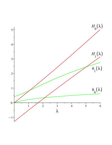
Figure 3. Eigencurves $H_{0}(\lambda),H_{1}(\lambda)$ (red) and $h_{0}(\lambda),h_{1}(\lambda)$ (green) for $a=3$, $b=2$, $c=1$.

When working with the boundary conditions $w(0)=w(\frac{1}{2}\pi)=0$ we use the basis $\sin(2n\tau)$, $n\in\mathbb{N}$. We obtain the corresponding matrix representations for $D,C,B$ from (8.4), (8.5), (8.6) by replacing $\cos$ by $\sin$ everywhere. Note that these matrix representations agree with those with respect to $\cos(2n\tau)$ when we delete the first row and first column of the latter, except for the three entries in the $i$th row and $j$th column with $(i,j)=(1,1),(1,2),(2,1)$. Similarly, when working with the boundary conditions $w^{\prime}(0)=w(\frac{1}{2}\pi)=0$ we use the basis $\cos((2n+1)\tau)$, $n\in\mathbb{N}_{0}$. The corresponding matrix representations are obtained from (8.4), (8.5), (8.6) by replacing $n$ by $n+\frac{1}{2}$. If the boundary conditions are $w(0)=w^{\prime}(\frac{1}{2}\pi)=0$ we use the basis $\sin((2n+1)\tau)$, $n\in\mathbb{N}_{0}$. The corresponding matrix representations are obtained from (8.4), (8.5), (8.6) by replacing $n$ by $n+\frac{1}{2}$ and $\cos$ by $\sin$. The matrix representations in the bases $\cos((2n+1)\tau)$ and $\sin((2n+1)\tau)$ only differ in the six positions $(i,j)=(1,1),(2,1),(1,2),(3,1),(2,2),(3,1)$.

9. Ellipsoids close to the unit sphere

In this section $k\in(0,1)$ is a fixed number and $k^{\prime}:=\sqrt{1-k^{2}}$. We consider the ellipsoid $\mathcal{E}(\epsilon)$ with semi-axes

$$a=(1+k^{2}\epsilon)^{1/2},\,b=1,\,c=(1-k^{\prime 2}\epsilon)^{1/2}\quad\text{for $0<\epsilon<(k^{\prime})^{-2}$}.$$

In the notation $\mathcal{E}(\epsilon)$ we suppressed the dependence of $\mathcal{E}(\epsilon)$ on $k$. The given number $k$ agrees with the number $k$ from (2.4) associated with $\mathcal{E}(\epsilon)$. If $\epsilon\to 0$ then $\mathcal{E}(\epsilon)$ approaches the unit sphere. The functions $p(s)$ and $q(t)$ from (4.3) and (4.4) become

$$p(s)=(1-k^{\prime 2}\epsilon\operatorname{cn}^{2}(s,k^{\prime}))^{1/2},\quad q(t)=(1+k^{2}\epsilon\operatorname{cn}^{2}(t,k))^{1/2}.$$

We denote the eigenvalue $\lambda_{m,n,\kappa}(a,b,c)$ for the ellipsoid $\mathcal{E}(\epsilon)$ by $\lambda_{m,n,\kappa}(\epsilon)$. Similarly, we denote the eigenvalue functions associated with (4.1), (4.2), (5.1), (5.2), (5.3) by $H_{m,\kappa}(\lambda,\epsilon)$ and $h_{n,\kappa}(\lambda,\epsilon)$, respectively. The corresponding two-parameter eigenvalue problems can be considered not only for $0<\epsilon<k^{\prime-2}$ but also for $-k^{-2}<\epsilon<k^{\prime-2}$. If $\epsilon=0$ we obtain the eigenvalue problem determining Lamé polynomials as mentioned in Section 6. In particular, $\lambda_{m,n,\kappa}(0)=\Lambda_{m,n,\kappa}$ with $\Lambda_{m,n,\kappa}$ given by (6.1).

Lemma 10.

Let $m,n\in\mathbb{N}_{0}$ and $\kappa\in\{0,1\}^{3}$. The eigenvalue functions $H_{m,\kappa}(\lambda,\epsilon)$ and $h_{n,\kappa}(\lambda,\epsilon)$ are analytic at $\lambda=\Lambda_{m,n,\kappa}$ and $\epsilon=0$. If $w(t)=W_{m,n,\kappa}(t)$ is a corresponding Lamé polynomial and $v(s)=w(K+iK^{\prime}-is)$ then

(9.1) $$\frac{\partial H_{m,\kappa}}{\partial\lambda}(\Lambda_{m,n,\kappa},0) = \frac{\int_{0}^{K^{\prime}}\operatorname{dn}^{2}(s,k^{\prime})v(s)^{2}\,ds}{\int_{0}^{K^{\prime}}v(s)^{2}\,ds},$$

(9.2) $$\frac{\partial H_{m,\kappa}}{\partial\epsilon}(\Lambda_{m,n,\kappa},0) = \frac{k^{\prime 2}\int_{0}^{K^{\prime}}\operatorname{cn}(s,k^{\prime})v(s)\frac{d}{ds}\left(\operatorname{cn}(s,k^{\prime})\frac{dv}{ds}\right)\,ds}{\int_{0}^{K^{\prime}}v(s)^{2}\,ds},$$

(9.3) $$\frac{\partial h_{n,\kappa}}{\partial\lambda}(\Lambda_{m,n,\kappa},0) = \frac{k^{2}\int_{0}^{K}\operatorname{sn}^{2}(t,k)w(t)^{2}\,dt}{\int_{0}^{K}w(t)^{2}\,dt},$$

(9.4) $$\frac{\partial h_{n,\kappa}}{\partial\epsilon}(\Lambda_{m,n,\kappa},0) = \frac{k^{2}\int_{0}^{K}\operatorname{cn}(t,k)w(t)\frac{d}{dt}\left(\operatorname{cn}(t,k)\frac{dw}{dt}\right)\,dt}{\int_{0}^{K}w(t)^{2}\,dt}.$$

Proof.

Consider a regular Sturm-Liouville problem of the form

(9.5) $$-\frac{d}{dt}\left(P(t,\mu)\frac{dw}{dt}\right)+Q(t,\mu)w=hR(t,\mu)w,\quad\alpha\leq t\leq\beta,$$

with separated boundary conditions at $t=\alpha$ and $t=\beta$ (we use only Neumann or Dirichlet conditions.) The eigenvalue parameter is $h$ and the perturbation parameter is $\mu$. The coefficient functions $P(t,\mu)$, $Q(t,\mu)$ and $R(t,\mu)$ are continuous with continuous partial derivatives $P_{\mu}$, $Q_{\mu}$ and $R_{\mu}$ with respect to $\mu$ for $t\in[\alpha,\beta]$ and $\mu$ is some interval $J$. Let $h(\mu)$ be the eigenvalue of this Sturm-Liouville problem determined by a fixed oscillation number of a corresponding eigenfunction $w(t,\mu)$. The eigenfunction $w(t,\mu)$ satisfies initial conditions at $t=\alpha$ that are independent of $\mu$. We differentiate (9.5) with respect to $\mu$, multiply by $w(t,\mu)$, and integrate from $t=\alpha$ to $t=\beta$. We obtain

(9.6) $$\frac{dh}{d\mu}\int_{\alpha}^{\beta}R(t,\mu)w(t,\mu)^{2}\,dt\\ =\int_{\alpha}^{\beta}\left(P_{\mu}(t,\mu)w^{\prime}(t,\mu)^{2}+(Q_{\mu}(t,\mu)-hR_{\mu}(t,\mu))w(t,\mu)^{2}\right)\,dt.$$

If we apply (9.6) to our eigenvalue problems (4.1), (4.2) with boundary conditions (5.1), (5.2), (5.3) and $\mu=\lambda$ we immediately obtain (9.1) and (9.3). If we apply (9.6) to (4.2), (4.6), (5.1) and $\mu=\epsilon$ then we obtain

$$\frac{\partial h_{n,\kappa}}{\partial\epsilon}(\lambda,0)=\frac{k^{2}\int_{0}^{K}\operatorname{cn}^{2}(t,k)\left(-w^{\prime}(t)^{2}+(\lambda k^{2}\operatorname{sn}^{2}(t,k)-h)w(t)^{2}\right)\,dt}{2\int_{0}^{K}w(t)^{2}\,dt},$$

where $\lambda=\Lambda_{m,n,\kappa}$. This gives (9.4) using Lamé’s differential equation

$$w^{\prime\prime}+(h-\lambda k^{2}\operatorname{sn}^{2}(t,k))w=0$$

and the identity

$$\operatorname{cn}^{2}(t,k)(-w^{\prime 2}+ww^{\prime\prime})=-\left(\operatorname{cn}^{2}(t,k)ww^{\prime}\right)^{\prime}+2\operatorname{cn}(t,k)w\left(\operatorname{cn}(t,k)w^{\prime}\right)^{\prime}.$$

Equation (9.2) is proved similarly. ∎

Theorem 11.

Let $m,n\in\mathbb{N}_{0}$ and $\kappa\in\{0,1\}^{3}$. The function $\lambda_{m,n,\kappa}(\epsilon)$ is analytic at $\epsilon=0$ with derivative

(9.7) $$\lambda_{m,n,\kappa}^{\prime}(0)=-\frac{\frac{\partial H_{m,\kappa}}{\partial\epsilon}(\Lambda_{m,n,\kappa},0)-\frac{\partial h_{n,\kappa}}{\partial\epsilon}(\Lambda_{m,n,\kappa},0)}{\frac{\partial H_{m,\kappa}}{\partial\lambda}(\Lambda_{m,n,\kappa},0)-\frac{\partial h_{n,\kappa}}{\partial\lambda}(\Lambda_{m,n,\kappa},0)},$$

where the four partial derivatives on the right are given in Lemma 10.

Proof.

The function $\lambda=\lambda_{m,n,\kappa}(\epsilon)$ solves

$$H_{m,\kappa}(\lambda,\epsilon)-h_{n,\kappa}(\lambda,\epsilon)=0,\quad\lambda(0)=\Lambda_{m,n,\kappa}.$$

It follows from (9.1), (9.3) that the partial derivative of $H_{m,\kappa}(\lambda,\epsilon)-h_{n,\kappa}(\lambda,\epsilon)$ with respect to $\lambda$ at the point $(\Lambda_{m,n,\kappa},0)$ is positive. Now the implicit function theorem for analytic functions shows that $\lambda(\epsilon)$ is analytic at $\epsilon=0$ and also gives (9.7). ∎

We introduce the differential operator

$$Au=\frac{k^{\prime 2}\operatorname{cn}(s,k^{\prime})\frac{\partial}{\partial s}\left(\operatorname{cn}(s,k^{\prime})\frac{\partial u}{\partial s}\right)-k^{2}\operatorname{cn}(t,k)\frac{\partial}{\partial t}\left(\operatorname{cn}(t,k)\frac{\partial u}{\partial t}\right)}{\operatorname{dn}^{2}(s,k^{\prime})-k^{2}\operatorname{sn}^{2}(t,k)}.$$

Then (9.7) becomes

$$\lambda^{\prime}_{m,n,\kappa}(0)=-\frac{\langle Au,u\rangle_{\mathcal{S}}}{\langle u,u\rangle_{\mathcal{S}}},$$

where $u=U_{m,n,\kappa}$ is the sphero-conal harmonic (6.2), and the inner product is

$$\langle u_{1},u_{2}\rangle_{\mathcal{S}}=\int_{-K^{\prime}}^{K^{\prime}}\int_{-2K}^{2K}(\operatorname{dn}^{2}(s,k^{\prime})-k^{2}\operatorname{sn}^{2}(t,k))u_{1}(s,t)u_{2}(s,t)\,dt\,ds.$$

Fix $\ell\in\mathbb{N}_{0}$ and $\kappa\in\{0,1\}^{3}$ such that $\ell-|\kappa|$ is nonnegative and even. Let $V$ denote the vector space of spherical harmonics homogeneous of degree $\ell$ with parity $\kappa$. The dimension $d$ of $V$ is $d=\frac{1}{2}(\ell-|\kappa|)+1$. Let $u_{1},u_{2},\dots,u_{d}$ be an orthonormal basis of $V$ with respect to the inner product $\langle\cdot,\cdot\rangle_{\mathcal{S}}$ consisting of sphero-conal harmonics. It is easy to see that $\langle Au_{i},u_{j}\rangle_{\mathcal{S}}=0$ if $i\neq j$, so the matrix $M_{1}$ with entries $\langle Au_{i},u_{j}\rangle_{\mathcal{S}}$ is diagonal and its diagonal entries are $-\lambda_{m,n,\kappa}^{\prime}(0)$ with $2m+2n+|\kappa|=\ell$.

The differential operator $A$ can be expressed in spherical coordinates and then agrees with the operator $A_{1}$ in [7] with $\alpha=\frac{1}{2}k^{2}$, $\beta=0$ and $\gamma=-\frac{1}{2}k^{\prime 2}$. It is shown in [7] that the matrix $M_{2}$ with entries $(\langle AU_{i},U_{j}\rangle_{\mathcal{S}})$ with $U_{1},U_{2},\dots,U_{d}$ denoting an orthonormal basis of $V$ derived from separation of variables in spherical coordinates is tridiagonal. This matrix $M_{2}$ is similar to the diagonal matrix $M_{1}$. Therefore, the derivatives $-\lambda_{m,n,\kappa}^{\prime}(0)$ with $2m+2n+|\kappa|=\ell$ are the eigenvalues of the matrix $M_{2}$. This shows that our formula (9.7) is consistent with [7, Theorem 4].

As an example, consider $\ell=2$ and $\kappa=(0,0,0)$. Then the dimension of $V$ is two. If $m=0$, $n=1$ the corresponding Lamé polynomial is [1, page 205]

$$w(t)=\operatorname{sn}^{2}(t,k)-\frac{1}{3k^{2}}\left(1+k^{2}+\sqrt{1-k^{2}k^{\prime 2}}\right).$$

If $m=1$, $n=0$ we obtain the corresponding Lamé polynomial by replacing $+\sqrt{1-k^{2}k^{2}}$ by $-\sqrt{1-k^{2}k^{\prime 2}}$. We find from (9.7)

$$\lambda^{\prime}_{0,1,(0,0,0)}(0) = 2-4k^{2}-\tfrac{8}{7}\sqrt{1-k^{2}k^{\prime 2}},$$

$$\lambda^{\prime}_{1,0,(0,0,0)}(0) = 2-4k^{2}+\tfrac{8}{7}\sqrt{1-k^{2}k^{\prime 2}}.$$

This result matches the result from [7].

References

- [1] F. M. Arscott. Periodic Differential Equations. The MacMillan Company, New York 1964.
- [2] F. V. Atkinson and A. B. Mingarelli. Multiparameter eigenvalue problems. Sturm-Liouville theory. CRC Press, Boca Raton, FL, 2011.
- [3] P. B. Bailey, W. N. Everett and A. Zettl. The SLEIGN2 Sturm-Liouville code. ACM Trans. Math. Software, 27 (2001), 143–192
- [4] P. Binding and H. Volkmer. Eigencurves of two-parameter Sturm-Liouville equations. SIAM Rev. 38 (1996), 27–48.
- [5] G. Dassios. Ellipsoidal Harmonics: Theory and Applications. Cambridge University Press, New York, 2012.
- [6] A. Erdélyi. Higher transcendental functions, Vol. III. McGraw-Hill, New York, 1955.
- [7] S. Eswarathasan and T. Kolokolnikov. Laplace–Beltrami spectrum of ellipsoids that are close to spheres and analytic perturbation theory. IMA J. Appl. Math. 87 (2021), 20–49.
- [8] E. Heine. Handbuch der Kugelfunctionen, Volume 1. G. Reimer Verlag, Berlin, 1878.
- [9] E. W. Hobson. The Theory of Spherical and Ellipsoidal Harmonics. Chelsea Publishing Company, New York, 1965,
- [10] E. L. Ince. Further investigations into the periodic Lamé functions. Proc. Royal Soc. Edinburgh, Sect. A. 60 (1940), 83–99.
- [11] J. Jost. Riemannian Geometry and Geoemtric Analysis. Springer-Verlag, Berlin Heidelberg New York, 2005.
- [12] G. Lamé. Memoire sur l’equilibre des temperatures dans un ellipsoide à trois axes inégaux. Jour. de Math. Pures et Appl. IV, 1839, 126–163.
- [13] F. W. Olver. Asymptotics and Special Functions. A K Peters, Natick, Massachusetts, 1997.
- [14] F. W. J. Olver, D. W. Lozier, F.F. Boisvert, and C. W. Clark, editors. em NIST handbook of mathematical functions. Cambridge University Press, Cambridge, 2010.
- [15] H. Volkmer. Multiparameter eigenvalue problems and expansion theorems, volume 1356 of Lecture Notes in Mathematics. Springer-Verlag, Berlin, 1988.
- [16] H. Volkmer. Eigenvalues of the Laplace-Beltrami operator on a prolate spheroid, J. Differential Equations 373 (2023), 411-445.
- [17] W. Walter. Ordinary Differential Equations. Graduate Texts in Mathematics 182, Springer-Verlag, New York, 1998.
- [18] E. T. Whittaker and G. N. Watson. A course of modern analysis. Cambridge University Press, Cambridge, 1927.