Integral representations and asymptotic expansions for the second type Neumann series of Bessel functions of the first kind

Abstract.

In this paper we study the following Bessel series $\sum_{l=1}^{\infty}{J_{l+m^{\prime}}(r)J_{l+m}(r)}{(l+\beta)^{\alpha}}$ for any $m,m^{\prime}\in\mathbb{Z}$, $\alpha\in\mathbb{R}$ and $\beta>-1$. They are a particular case of the second type Neumann series of Bessel functions of the first kind. More specifically, we derive fully explicit integral representations and study the asymptotic behavior with explicit terms. As a corollary, the asymptotic behavior of series of the derivatives of Bessel functions can be understood.

1. Introduction.

Bessel functions of the first kind and order $\nu$ can be defined as

$$J_{\nu}(x)=\sum_{n=0}^{\infty}\frac{(-1)^{n}}{n!\Gamma(n+\nu+1)}\left(\frac{x}{2}\right)^{2n+\nu}\,.$$

As is well-known, they are a particular solution of the Bessel differential equation,

$$x^{2}y^{\prime\prime}(x)+xy^{\prime}(x)+(x^{2}-\nu^{2})y(x)=0\,.$$

Bessel functions are ubiquitous functions in (applied) mathematics and theoretical physics. In particular, these series of Bessel functions appear frequently and they have been studied in detail, [10, Chapters XVI-XIX].

In this paper we are interested in the second type Neumann series of Bessel functions of the first kind, [2, Section 2.5],

$$\mathfrak{N}^{a,b}_{\mu,\nu}(x)\coloneqq\sum_{n\geq 1}\alpha_{n}J_{\mu+an}(x)J_{\nu+bn}(x)\,,$$ (1.1)

being all parameters real numbers. Classical examples of these series are von Lommel’s series and the Al-Salam series, see [2, Section 2.5] and references therein. Here we want to study the case of $a=b=1$ and

$$\alpha_{n}=(n+\beta)^{\alpha}\,,$$

for $\alpha\in\mathbb{R}$ and $\beta>-1$. That is,

$$S_{\alpha,\beta,m,m^{\prime}}(r)\coloneqq\sum_{l=1}^{\infty}{J_{l+m^{\prime}}(r)J_{l+m}(r)}{(l+\beta)^{\alpha}}.$$ (1.2)

Classical examples of these series are consequences of Neumann’s Addition Theorem, see [8, (10.23.3),(10.23.4)],

$$\sum_{k=0}^{2n}(-1)^{k}J_{k}(r)J_{2n-k}(r)+2\sum_{l=1}^{\infty}J_{l}(r)J_{l+2n}(r) =0,$$

$${J_{0}}^{2}\left(z\right)+2\sum_{k=1}^{\infty}{J_{k}}^{2}\left(z\right) =1,$$

for $n\geq 1$. Furthermore, from this theorem one can easily derive exact formulas for derivatives of Bessel functions, see [4, Appendix B]. For instance,

$$\sum_{l=0}^{\infty}{\epsilon_{l}}J_{l}^{\prime}(r)^{2} =\frac{1}{2}\,,\quad\sum_{l=0}^{\infty}{\epsilon_{l}}l^{2}J_{l}(r)J_{l}^{\prime}(r)=\frac{r}{4}\,,\quad\sum_{l=0}^{\infty}{\epsilon_{l}}l^{4}J_{l}(r)^{2}=\frac{r^{2}(4+3r^{2})}{8}\,,$$

where $\epsilon_{l}:=2-\delta_{l,0}$ is Neumann’s factor. Another classical example is the following Turán type inequality for all $x\in\mathbb{R}$ and $\nu>-1$, [9, p. 384],

$$\Delta_{\nu}(x)=J_{\nu}^{2}(x)-J_{\nu-1}(x)J_{\nu+1}(x)\geqslant 0\,,$$ (1.3)

where

$$\Delta_{\nu}(x)\coloneqq\frac{1}{\nu+1}J_{\nu}^{2}(x)+\frac{2}{\nu+2}J_{\nu+1}^{2}(x)+2\nu\sum_{n\geqslant 2}\frac{J_{\nu+n}^{2}(x)}{(\nu+n-1)(\nu+n+1)}.$$ (1.4)

Recently, these series have appeared in the study of critical points of random fields satisfying the Helmholtz equation on the plane, [4]. This is expected as, by definition, the random field $u$ is

$$u:=\sum_{l}a_{l}\,\sigma_{l}\,e^{il\theta}\,J_{l}(r)\,,\qquad\sigma_{l}:=\begin{cases}|l|^{-s}&\text{if }l\neq 0\,,\\ 0&\text{if }l=0\,,\end{cases}$$ (1.5)

where the real and imaginary parts of $a_{l}$ are independent standard Gaussian random variables subject to the constraint $a_{l}=(-1)^{l}\overline{a_{-l}}$ (which makes $u$ real valued), $(r,\theta)\in\mathbb{R}^{+}\times\mathbb{T}$ are the polar coordinates. Therefore, the (co)variance kernel of the random function (1.5) is

$$K(r,\theta):=\mathbb{E}[u(r,\theta)\,u(r,\theta)]=4\sum_{l=1}^{\infty}l^{-2s}J_{l}(r)J_{l}(r)\,,$$

see [4, Remark 4.2]. The covariance kernel is one of the main inputs in the Kac-Rice formula, e.g. [1], which can be used to compute the expected value of the number of critical points in a given region. There, a method to compute the asymptotics of $\mathcal{J}_{s,m,m^{\prime}}(r)\coloneqq S_{-2\alpha,\beta=0,m,m^{\prime}}(r)$ is given. The basic idea of the strategy is to decompose the series as follows

$$\mathcal{J}_{s,m,m^{\prime}}(r)=\mathcal{J}^{\textnormal{I}}_{s,m,m^{\prime}}(r)+\mathcal{J}^{\textnormal{II}}_{s,m,m^{\prime}}(r)+\mathcal{J}^{\textnormal{III}}_{s,m,m^{\prime}}(r)\,,$$

where (for some $\delta>0$ small):

• I only involves “frequencies” $\lambda\coloneqq l/r$ smaller than $(1-\delta)$,

• II involves $\lambda$ close to 1 (more precisely, $|\lambda-1|<2\delta$), and

• III involves $\lambda$ larger than $(1+\delta)$.

Then, different oscillatory techniques are used in each region to extract the leading term and control the errors. This is done for every $\alpha$, using different techniques for different regions of this parameter.

A completely different approach is followed here. First, we divide the series between $\alpha\geq 0$ and $\alpha<0$ and derive integral representations in the latter case. Once we have those integral representations, we use different asymptotic techniques from harmonic analysis (such as the stationary phase method and the Hankel transform) to compute their asymptotic expansions. Finally, the case of $\alpha\geq 0$ is treated using a “trick” (Lemma 5.1) to reduce it to the previous case. This method allow us to obtain both integral representations and asymptotic expansions.

Beyond the fact that the methods used are different, we believe there are also some worth noting improvements. First, the series considered are more general as the parameter $\beta$ can take any value in $(-1,+\infty)$, not just $0$. Second, we also provide integral representations, which is an important result by itself and can be useful for other purposes apart from asymptotic expansions when $r\to\infty$. See [2, Section 2.5] and references therein for some literature on other integral representations for these types of series. Third, our method allows us to compute the whole asymptotic expansion, not just the leading term. For the sake of simplicity, we have basically limited our attention to the first terms, but using Remark 4.2 and 4.7 obtaining higher order terms is straightforward. In fact, in Proposition 4.6 second order terms are easily computed for convenience (they are needed for the case of $\alpha=0$). This also results in a better understanding of the asymptotics for some series of derivatives of Bessel functions. Comparing [4, Corollary 3.7] with Corollary 6.3 here, we can see, e.g., the following improvement,

$$\sum_{l=1}^{\infty}\frac{J_{l}(r)J^{\prime}_{l}(r)}{l}=O\left(r^{-1}\right)\Rightarrow\sum_{l=1}^{\infty}\frac{J_{l}(r)J^{\prime}_{l}(r)}{l+\beta}=-\frac{\Phi(-1,1,\beta+1)\cos(2r)}{\pi r}+o(r^{-1})\,,$$

where $\Phi$ is the Lerch transcendent function. The organization and main results of this paper are as follows. Relevant notation is introduced in Section 2. In Section 3 we derive the integral representations for $\alpha<0$. In particular, for $\mu\in\mathbb{Z}_{\geq 0}$, we define

$$F_{\alpha,\beta,\mu}(\varphi)\coloneqq-\frac{1}{2}e^{-i\varphi(\mu+2)}\left(e^{2i\varphi(\mu+2)}\Phi\left(-e^{2i\varphi},\alpha,\beta+1\right)+\Phi\left(-e^{-2i\varphi},\alpha,\beta+1\right)\right)\,,$$

where, as above, $\Phi$ is the Lerch transcendent function defined in Section 2.

Theorem 1.1.

Let $\alpha,\beta+1>0$ and $m,m^{\prime}=0,1,\ldots$, then the series (3.1) can be expressed in the following integral forms:

$$\sum_{l=1}^{\infty}\frac{J_{l+m^{\prime}}(r)J_{l+m}(r)}{(l+\beta)^{\alpha}}=\frac{2i^{-\mu}}{\pi^{2}}\int_{0}^{\pi/2}\int_{0}^{\pi}e^{i2r\cos\varphi\cos\theta}F_{\alpha,\beta,\mu}(\varphi)\cos(\nu\theta)d\varphi d\theta\,,$$ (1.6)

as a two-dimensional exponential oscillatory integral and

$$\sum_{l=1}^{\infty}\frac{J_{l+m^{\prime}}(r)J_{l+m}(r)}{(l+\beta)^{\alpha}}=\frac{(-1)^{m^{\prime}}}{\pi}\int_{0}^{\pi}\,J_{\nu}(2r\cos\varphi)F_{\alpha,\beta,\mu}(\varphi)d\varphi\,,$$ (1.7)

as a one-dimensional Hankel transform, for $r\in\mathbb{R}$ where $\mu\coloneqq m+m^{\prime}$ and $\nu\coloneqq m-m^{\prime}$.

Using both integral representations, in Section 4 we are able to compute its asymptotic expansion. In particular,

Theorem 1.2.

Let $\mu\coloneqq m+m^{\prime}$ and $\nu\coloneqq m-m^{\prime}$. If $\alpha>0$ and $\alpha\notin\mathbb{N}$, then there are constants $c$ such that

$$\sum_{l=1}^{\infty}\frac{J_{l+m^{\prime}}(z)J_{l+m}(z)}{(l+\beta)^{\alpha}}=\frac{c^{1}_{\alpha,\nu}}{r^{\alpha}}+\frac{c^{2}_{\alpha,\beta,\nu}+c^{3}_{\alpha,\beta}\sin\left(2r-{\pi\mu}/{2}\right)}{r}+O\left(\frac{1}{r^{\gamma}}\right)\,,$$

with $\gamma\coloneqq\min\{\alpha+1,2\}$, see Corollary 4.4 for explicit constants. Now let $\alpha\in\mathbb{N}$. Similarly for $\alpha=1$,

$$\sum_{l=1}^{\infty}\frac{J_{l+m^{\prime}}(z)J_{l+m}(z)}{(l+\beta)}=\frac{c^{4}_{\nu}\log r}{r}+\frac{c^{5}_{\beta,\nu}+c^{3}_{1,\beta}\sin\left(2r-{\pi\mu}/{2}\right)}{r}+o\left(r^{-1}\right)\,,$$

and for $\alpha>1$,

$$\sum_{l=1}^{\infty}\frac{J_{l+m^{\prime}}(z)J_{l+m}(z)}{(l+\beta)^{\alpha}}= \frac{c^{2}_{\alpha,\beta,\nu}+c^{3}_{\alpha,\beta}\sin\left(2r-{\pi\mu}/{2}\right)}{r}+O\left(\frac{1}{r^{2-\gamma}}\right)\,,$$

with $\gamma>0$ arbitrarily small, see Corollary 4.8 for explicit constants.

In Section 5, first we derive the asymptotics for $S_{\alpha,\beta,\mu,\nu}(r)$ when $\alpha\geq 0$. In particular,

Theorem 1.3.

For $\alpha\geq 0$ and $\beta,\mu,\nu$ as above,

$$\sum_{l=1}^{\infty}{J_{l+m^{\prime}}(z)J_{l+m}(z)}{(l+\beta)^{\alpha}}={c^{1}_{-\alpha,\nu}}r^{\alpha}+o(r^{\alpha})=\frac{2^{-\alpha-1}\Gamma(\alpha+1)r^{\alpha}}{\Gamma\left(\frac{1}{2}(-\nu+\alpha+2)\right)\Gamma\left(\frac{1}{2}(\nu+\alpha+2)\right)}+o(r^{\alpha})\,,$$

where the coefficient must be understood as the continuous extension for the values of $\alpha$ where it is undefined.

In Proposition 5.3 integral representations for this case are given. Finally, in Section 6, we derive asymptotic formulas for series of derivatives of Bessel functions.

2. Notation.

With $\Phi$ we denote the Lerch transcendent function, i.e.,

$$\Phi(z,\alpha,\beta)=\sum_{n=0}^{\infty}\frac{z^{n}}{(\beta+n)^{\alpha}}\,,$$

for $|z|<1$ (or $|z|\leq 1$ if $\alpha>1$), see [8, 25.14.1], and for other values it is extended by analytic continuation. As a particular case we have $\text{Li}_{\alpha}$, the polylogarithm of order $\alpha$. The function $\text{Li}_{\alpha}(z)$ is defined as a series

$$\mathrm{Li}_{\alpha}\left(z\right)=\sum_{n=1}^{\infty}\frac{z^{n}}{n^{\alpha}}\,,$$ (2.1)

for $|z|<1$ (or $|z|\leq 1$ if $\alpha>1$), see [8, 25.12.10], and for other values it is extended by analytic continuation. We have that

$$\mathrm{Li}_{\alpha}\left(z\right)=z\Phi\left(z,\alpha,1\right)\,.$$

Also, the family of Struve functions is denoted by $\textnormal{\boldsymbol{H}}_{\nu}(z)$. Recall that Struve functions are particular solutions of the non-homogeneous Bessel’s differential equation

$$\frac{{d}^{2}y}{{dz}^{2}}+\frac{1}{z}\frac{dy}{dz}+\left(1-\frac{\nu^{2}}{z^{2}}\right)y=\frac{(\tfrac{1}{2}z)^{\nu-1}}{\sqrt{\pi}\Gamma\left(\nu+\tfrac{1}{2}\right)}$$

defined by the power-series expansion

$$\textnormal{\boldsymbol{H}}_{\nu}(z)\coloneqq(\tfrac{1}{2}z)^{\nu+1}\sum_{n=0}^{\infty}\frac{(-1)^{n}(\tfrac{1}{2}z)^{2n}}{\Gamma\left(n+\tfrac{3}{2}\right)\Gamma\left(n+\nu+\tfrac{3}{2}\right)}.$$

The $(p,q)$-regularized hypergeometric function will be denoted by ${}_{p}\tilde{F}_{q}$.

3. Integral representations for Bessel series

The purpose of this section is give an integral representation of

$$S_{-\alpha,\beta,m,m^{\prime}}(r)\coloneqq\sum_{l=1}^{\infty}\frac{J_{l+m^{\prime}}(r)J_{l+m}(r)}{(l+\beta)^{\alpha}}\,,$$ (3.1)

where $m,m^{\prime}=0,1,\dots$, $\alpha>0$ and $\beta>-1$ so that $l+\beta>0$. For this we need some definitions. We define, for $\mu\in\mathbb{Z}_{\geq 0}$,

$$F_{\alpha,\beta,\mu}(\varphi)\coloneqq-\frac{1}{2}e^{-i\varphi(\mu+2)}\left(e^{2i\varphi(\mu+2)}\Phi\left(-e^{2i\varphi},\alpha,\beta+1\right)+\Phi\left(-e^{-2i\varphi},\alpha,\beta+1\right)\right)\,,$$

where $\Phi$ is the Lerch transcendent function defined in Section 2. A particular interesting situation is

$$F_{\alpha,m}(\varphi)\coloneqq F_{\alpha,0,m}(\varphi)=\frac{1}{2}\left(e^{i\varphi m}\text{Li}_{\alpha}\left(-e^{2i\varphi}\right)+e^{-i\varphi m}\text{Li}_{\alpha}\left(-e^{-2i\varphi}\right)\right)\,,$$

where $\text{Li}_{\alpha}$ is the polylogarithm of order $\alpha$ defined in Section 2. Before the main proposition of this section, let us study the function $F_{\alpha,m}$, in particular, its series expansion.

Lemma 3.1.

For $0\leq\varphi<\pi/2$, $\alpha>0$ and $\mu\in\mathbb{Z}_{\geq 0}$, we have

$$F_{\alpha,\beta,\mu}(\varphi)=\sum_{l=1}^{\infty}\frac{(-1)^{l}\cos(\varphi(\mu+2l))}{(l+\beta)^{\alpha}}=(-1)^{\mu}F_{\alpha,\beta,\mu}(\pi-\varphi)\,,$$ (3.2)

where the equality is true for $\varphi=\pi/2$ if $\alpha>1$. $F_{\alpha,\beta,\mu}$ is a smooth function for $0\leq\varphi<\pi/2$ and, possibly, with singularities at $\varphi=\pi/2$ if $\alpha\leq 1$. The same singularities can appear for the derivatives if $\alpha>1$.

Proof.

By (2.1) and the comments below, the only non-trivial case to consider is $0<\alpha\leq 1$ as the values of our interest ($z=-e^{i2\varphi}$) are on the boundary of the disk of convergence of the series, i.e., $z\in\partial D\backslash D$ where $D$ is the disk of convergence. First note that the following geometric sum gives

$$A_{N}(\rho,\varphi)\coloneqq\sum_{n=1}^{N}(-1)^{n}\rho^{n}e^{i\varphi 2n}=\frac{\rho e^{2i\varphi}\left(-1+(-\rho)^{N}e^{2iN\varphi}\right)}{1+\rho e^{2i\varphi}}\,,$$ (3.3)

where $\rho\in[0,1]$. Thus

$$|A_{N}(\rho,\varphi)|\leq\frac{2}{|1+\rho e^{2i\varphi}|}\leq M_{\delta}$$

for $\varphi\in[-\frac{\pi}{2}+\delta,\frac{\pi}{2}-\delta],\leavevmode\nobreak\ \forall\hskip 2.84526pt\delta>0$. Obviously this constant blows up as $\delta\to 0$. Hence, if

$$S_{N}(\rho,\varphi)\coloneqq\sum_{n=1}^{N}\frac{i^{-2n}\rho^{n}e^{i\varphi 2n}}{(n+\beta)^{\alpha}}\,,$$

by summation by parts for $n>m$,

$$|S_{n}-S_{m}|(\rho,\varphi) =\left|\frac{A_{n}(\rho,\varphi)}{(n+\beta)^{\alpha}}-\frac{A_{m}(\rho,\varphi)}{(m+\beta)^{\alpha}}+\sum_{k=m}^{n-1}A_{k}(\rho,\varphi)\left(\frac{1}{(k+\beta)^{\alpha}}-\frac{1}{(k+1+\beta)^{\alpha}}\right)\right|\leq$$

$$\leq M_{\delta}\left(\frac{1}{(n+\beta)^{\alpha}}+\frac{1}{(m+\beta)^{\alpha}}+\frac{1}{(m+\beta)^{\alpha}}-\frac{1}{(n+\beta)^{\alpha}}\right)=\frac{2M_{\delta}}{(m+\beta)^{\alpha}},$$

where the last inequality follows from a telescopic cancellation. As the RHS goes to zero as $m\to\infty$, the sequence is Cauchy and

$$|S(\rho,\varphi)-S_{m}((\rho,\varphi))|<\varepsilon$$

for $m>\left(2M_{\delta}/\varepsilon\right)^{\frac{1}{\alpha}}-\beta$, independent of $\rho,\varphi$. Thus, the convergence is uniform so $S(\rho,\varphi)$ is continuous if $\varphi\neq\frac{\pi}{2}$. For $\rho<1$, $S(\rho,\varphi)=\rho\left(-e^{2i\varphi}\right)\Phi\left(-e^{2i\varphi}\rho,\alpha,\beta+1\right)$ (by the definition of $\Phi$ as a series). Also, for $\varphi\in[-\frac{\pi}{2}+\delta,\frac{\pi}{2}-\delta]$ we have $S(1,\varphi)=-e^{2i\varphi}\Phi\left(-e^{2i\varphi},\alpha,\beta+1\right)$ (understood as the analytic continuation of $\Phi$ for $\rho<1$). As $\delta>0$ is arbitrary, the proof of the series expansion follows straightforwardly taking the real part, i.e.,

$$\sum_{l=1}^{\infty}\frac{(-1)^{l}\cos(\varphi(\mu+2l))}{(l+\beta)^{\alpha}} =\sum_{l=1}^{\infty}\frac{\operatorname{Re}\left(e^{i\varphi\mu}(-e^{i2\varphi})^{l}\right)}{(l+\beta)^{\alpha}}=$$

$$=\operatorname{Re}\left(-e^{i\varphi(\mu+2)}\Phi\left(-e^{2i\varphi},\alpha,\beta+1\right)\right)=F_{\alpha,\beta,m}(\varphi)\,.$$

The parity property follows straightforwardly from the series expansion.

We have the following integral representation [8, 25.14.5]

$$\Phi\left(-e^{2i\varphi},\alpha,\beta+1\right)=\frac{1}{\Gamma(\alpha)}\int_{0}^{\infty}\frac{t^{\alpha-1}e^{-t(\beta+1)}}{1+e^{-t+2i\varphi}}\,dt\,,$$ (3.4)

so we might have singularities at $\varphi=\frac{\pi}{2}$ if $\alpha\leq 1$ and the function is $C^{\infty}$ except at $\varphi=\frac{\pi}{2}$. This is even true if $\alpha>1$ as

$$\frac{\partial\text{Li}_{\alpha}\left(-e^{\pm 2i\varphi}\right)}{\partial\varphi}=\pm 2i\text{Li}_{\alpha-1}\left(-e^{\pm 2i\varphi}\right),$$

$$\frac{\partial\Phi\left(-e^{2i\varphi},\alpha,\beta+1\right)}{\partial\varphi}=2i\left(\Phi\left(-e^{2i\varphi},\alpha-1,\beta+1\right)-(\beta+1)\Phi\left(-e^{2i\varphi},\alpha,\beta+1\right)\right)\,.$$

∎

See Figure 1 for some representations.

Remark 3.2.

Obviously the analytic continuation and the sum can differ on the boundary (the region of interest), that is why we need to check that they coincide. For instance, taking $\beta=0$ for simplicity, this is clear for $\alpha=0$ where the partial sums are given by (3.3) and they are not convergent for $\rho=1$. Nevertheless, the analytic continuation is well-defined and equals

$$\mathrm{Li}_{0}(-e^{2i\varphi})=\frac{-e^{i(\varphi(m+2))}}{1+e^{2i\varphi}}.$$

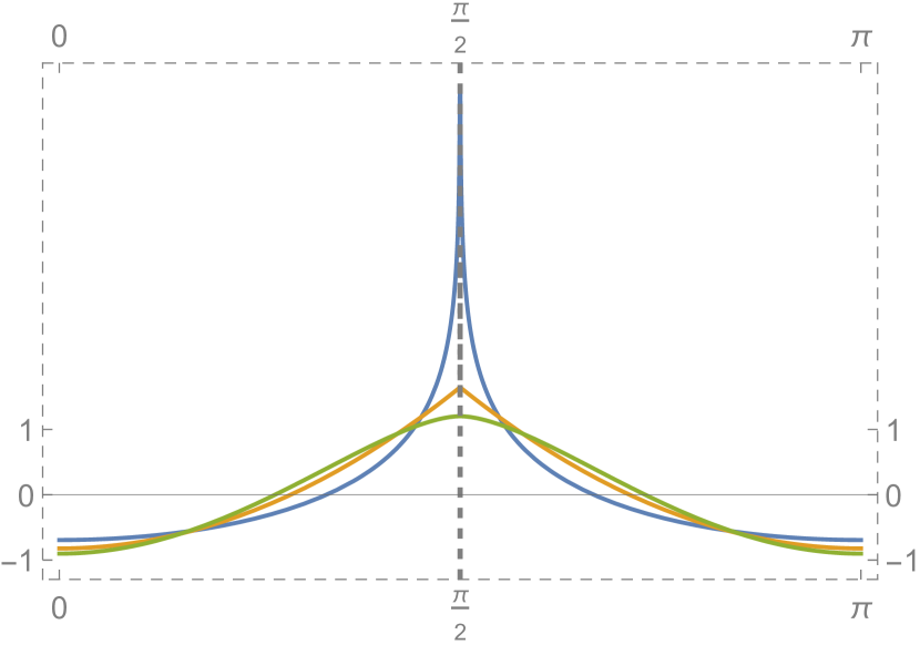
(a) Representation of $F_{\alpha,0}$ for several values of $\alpha$.

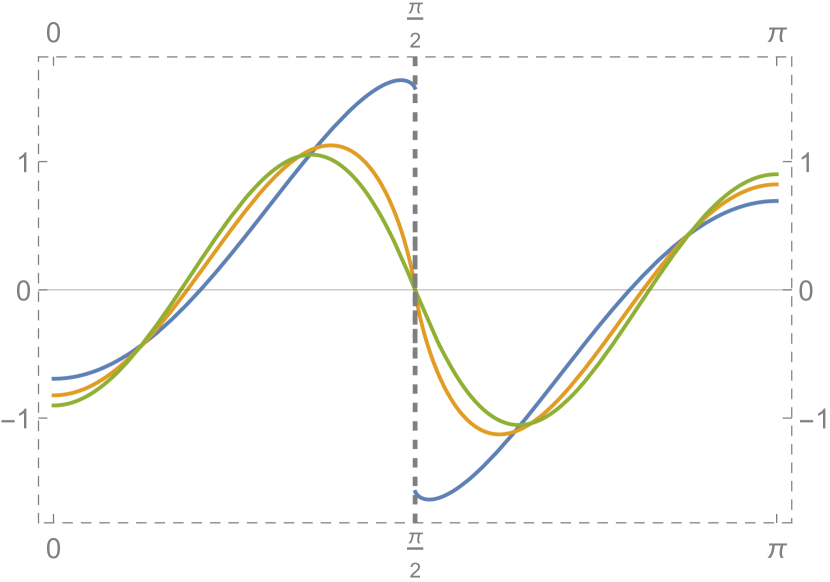
(b) Representation of $F_{\alpha,1}$ for several values of $\alpha$.

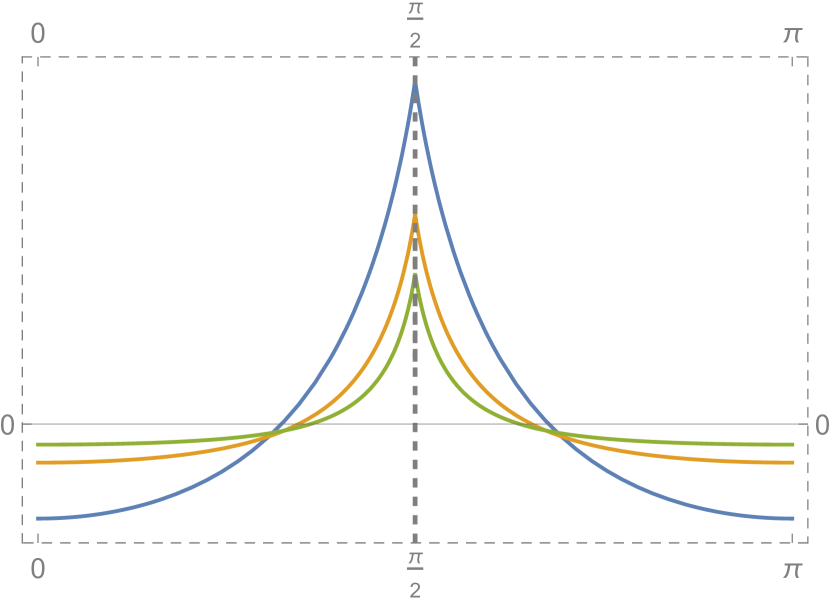
(c) Representation of $F_{2,\beta,0}$ for several values of $\beta$.

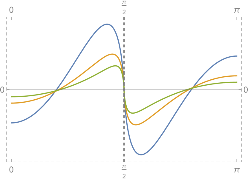
(d) Representation of $F_{2,\beta,0}$ for several values of $\beta$.

Figure 1. Representations of $F_{\alpha,\beta,\mu}$ for different parameters. The dashed line represents $\varphi=\pi/2$.

We are ready to prove the main theorem of this section.

Proof of Theorem 1.1.

First, we know that for $z\in\mathbb{C}$ [8, 10.9.26]

$$J_{\mu}\left(z\right)J_{\nu}\left(z\right)=\frac{2}{\pi}\int_{0}^{\pi/2}J_{\mu+\nu}\left(2z\cos\theta\right)\cos\left((\mu-\nu)\theta\right)d\theta\,,$$

if $\operatorname{Re}(\mu+\nu)>-1.$ Second, we also know that [8, 10.9.2]

$$J_{n}\left(z\right)=\frac{1}{\pi}\int_{0}^{\pi}\cos\left(z\sin\varphi-n\varphi\right)d\varphi=\frac{i^{-n}}{\pi}\int_{0}^{\pi}e^{iz\cos\varphi}\cos\left(n\varphi\right)d\varphi\,,$$ (3.5)

for $n\in\mathbb{Z}$. From these two expressions we obtain

$$J_{l+m^{\prime}}\left(z\right)J_{l+m}\left(z\right)=\frac{2i^{-\mu}}{\pi^{2}}\int_{0}^{\pi/2}\int_{0}^{\pi}e^{i2z\cos\varphi\cos\theta}(-1)^{l}\cos\left((2l+\mu)\varphi\right)\cos\left(\nu\theta\right)d\varphi d\theta\,.$$

Thus, if we can interchange the integral and the series we will have:

$$\sum_{l=1}^{\infty}\frac{J_{l+m^{\prime}}(z)J_{l+m}(z)}{(l+\beta)^{\alpha}}=\frac{2i^{-\mu}}{\pi^{2}}\int_{0}^{\pi/2}\int_{0}^{\pi}e^{i2z\cos\varphi\cos\theta}F_{\alpha,\beta,\mu}(\varphi)\cos(\nu\theta)d\varphi d\theta,$$

where we have used Lemma 3.1. To justify the swap, note that $F_{\alpha,\beta,\mu}$ can be written as

$$F_{\alpha,\beta,\mu}(\varphi)=\frac{1}{2}e^{-i\varphi\mu}\sum_{l=1}^{\infty}(-1)^{l}(l+\beta)^{-\alpha}e^{-i2l\varphi}+\frac{1}{2}e^{+i\varphi\mu}\sum_{l=1}^{\infty}(-1)^{l}(l+\beta)^{-\alpha}e^{i2l\varphi},$$

i.e., as a Fourier series. Hence, the swap will be justified if we can ensure this series converges in $L^{p}$ for some $p\geq 1$. Indeed, if $S_{N}$ denotes the $N$-partial sum of the Fourier series,

$$\left|\int_{0}^{\pi/2}\int_{0}^{\pi}e^{i2r\cos\varphi\cos\theta}\left(\sum_{l=N+1}^{\infty}\frac{(-1)^{l}\cos\left((2l+\mu)\varphi\right)}{(l+\beta)^{\alpha}}\right)\cos(\nu\theta)d\varphi d\theta\right|\lesssim$$ (3.6)

$$\hskip 199.16928pt\lesssim\left\lVert F_{\alpha,\beta,\mu}-S_{N}\right\rVert_{L^{1}([0,\pi])}\lesssim\left\lVert F_{\alpha,\beta,\mu}-S_{N}\right\rVert_{L^{p}([0,\pi])}\,,$$

for $p>1$. This is clear for $p=2$ and $\alpha>1/2$ as then

$$\sum_{l=1}^{\infty}\frac{1}{(l+\beta)^{2\alpha}}<\infty\,,$$

but a more detailed analysis of the function, not only the coefficients, is needed for $\alpha\in(0,1/2)$ (the function might have singularities at $\varphi=\pi/2$ by Lemma 3.1). From the series representation, [3, p. 29],

$$\Phi(z,s,a)=z^{-a}\Gamma(1-s)\log^{s-1}\left(\frac{1}{z}\right)+z^{-a}\left(\sum_{k=0}^{\infty}\frac{\log^{k}(z)\zeta(s-k,a)}{k!}\right)\text{ if }\neg(s\in\mathbb{Z}\land s>0)$$ (3.7)

for $|\log z|<2\pi$ where $\zeta$ is the (analytic continuation) of the Hurwitz zeta function, we can conclude (after a lengthy but straightforward computation)

$$|F_{\alpha,\beta,\mu}(\varphi)|\sim_{\alpha,\mu}|\pi/2-\varphi|^{\alpha-1}\,.$$

More precisely,

$$F_{\alpha,\beta,\mu}(\varphi)\sim\begin{cases}\frac{1}{2}\Gamma(1-\alpha)\left(-(\pi-2\varphi)^{\alpha-1}\right)\left(-2\sin\left(\frac{1}{2}\pi(\mu+\alpha)\right)\right)&\text{ if }\varphi\in(0,\frac{\pi}{2})\,,\\ \frac{1}{2}\Gamma(1-\alpha)(2\varphi-\pi)^{\alpha-1}\left(-2\sin\left(\frac{1}{2}\pi(\mu-\alpha)\right)\right)&\text{ if }\varphi\in(\frac{\pi}{2},\pi)\,.\\ \end{cases}$$

So $F_{\alpha,\beta,\mu}\in L^{p}([0,\pi])$ if $1<p<\frac{1}{1-\alpha}$. Then, by standard harmonic analysis [6, page 59], the convergence of the Fourier series is in $L^{p}([0,\pi])$. This proves (1.6).

In order to prove (1.7), by Fubini’s Theorem,

$$J_{l+m^{\prime}}\left(z\right)J_{l+m}\left(z\right)=\frac{2i^{-\mu}}{\pi^{2}}\int_{0}^{\pi}\int_{0}^{\pi/2}e^{i2z\cos\varphi\cos\theta}(-1)^{l}\cos\left((2l+\mu)\varphi\right)\cos\left(\nu\theta\right)d\theta d\varphi.$$

Thus, arguing as in (3.6) we conclude that:

$$\sum_{l=1}^{\infty}\frac{J_{l+m^{\prime}}(z)J_{l+m}(z)}{(l+\beta)^{\alpha}}=\frac{2i^{-\mu}}{\pi^{2}}\int_{0}^{\pi}\int_{0}^{\pi/2}e^{i2z\cos\varphi\cos\theta}\cos(\nu\theta)F_{\alpha,\beta,\mu}(\varphi)d\theta d\varphi.$$ (3.8)

By (3.5) splitting the integral from $0$ to $\pi/2$ and $\pi/2$ to $\pi$ with the change of variables $\varphi^{\prime}=\pi-\varphi$ in the latter case, we obtain for $z^{\prime}\in\mathbb{C}$ and even $\nu$

$$\int_{0}^{\frac{\pi}{2}}\cos(\theta\nu)\cos(z^{\prime}\cos\theta)\,d\theta=\frac{i^{\nu}\pi}{2}J_{\nu}(z^{\prime})\,,$$

and for odd $\nu$

$$\int_{0}^{\frac{\pi}{2}}\cos(\theta\nu)\sin(z^{\prime}\cos\theta)\,d\theta=\frac{i^{\nu-1}\pi}{2}J_{\nu}(z^{\prime})\,.$$

If we take $z=r$ real, then the RHS of 3.8 must be real. By definition, $\mu=\nu$ mod 2, so using

$$\int_{0}^{\pi/2}e^{iz^{\prime}\cos\theta}\cos(\nu\theta)d\theta=\int_{0}^{\pi/2}\cos(z^{\prime}\cos\theta)\cos(\nu\theta)d\theta+i\int_{0}^{\pi/2}\sin(z^{\prime}\cos\theta)\cos(\nu\theta)d\theta$$

for $z^{\prime}=2z\cos\varphi$, if $\mu$ is even (and so is $\nu$), $i^{-\mu}\in\mathbb{R}$, so the real part will be given by the cosine integral. The same, mutatis mutandis, for $\mu$ odd. ∎

Remark 3.3.

In our situation, interchanging the series and the integral sign can fail, so checking that a sufficient condition holds is necessary. For instance, as we saw in Remark 3.2, $F_{0,\mu}$ is well-defined, in fact, after a bit of trigonometry it equals:

$$F_{0,\mu}(\varphi)=-\frac{\cos((\mu+1)\varphi)}{2\cos\varphi}.$$

But it is well-know, as we will see below, that (taking $\mu=0$)

$$\sum_{l=1}^{\infty}J_{l}(r)^{2}=\frac{1}{2}-\frac{J_{0}(r){}^{2}}{2}.$$

But $F_{0,0}(\varphi)=-\frac{1}{2}$, and the integral representation that the proposition above would give (if the interchange of sum and integral were allowed) is false. For instance, as we will see in the next section, the integral representation would go to zero as $r\to\infty$ but the series goes to $\frac{1}{2}$. Also note that for that value of $\alpha$ our argument for a sufficient condition fails as there is no $p$ such that $1<p<\frac{1}{1-0}$.

Remark 3.4.

Let us briefly discuss the case $z\in\mathbb{C}$. For the sake of simplicity consider $m^{\prime}=\beta=0$. If $z\in\mathbb{C}$ we will have:

$$\sum_{l=1}^{\infty}\frac{J_{l}(z)J_{l+m}(z)}{l^{\alpha}} =\frac{i^{-m}}{\pi}\int_{0}^{\pi}\,{}_{1}\tilde{F}_{2}\left(1;1-\frac{m}{2},\frac{m}{2}+1;-\frac{(2z\cos\varphi)^{2}}{4}\right)F_{\alpha,m}(\varphi)d\varphi+$$

$$+\frac{i^{-m+1}}{\pi}\frac{z}{2}\int_{0}^{\pi}\cos\varphi\cdot\,_{1}\tilde{F}_{2}\left(1;\frac{3-m}{2},\frac{m+3}{2};-\frac{(2z\cos\varphi)^{2}}{4}\right)F_{\alpha,m}(\varphi)d\varphi.$$

Indeed, we can use

$$\int_{0}^{\pi/2}e^{iz^{\prime}\cos\theta}\cos(m\theta)d\theta =\frac{1}{2}\pi\cdot\,_{1}\tilde{F}_{2}\left(1;1-\frac{m}{2},\frac{m}{2}+1;-\frac{z^{\prime 2}}{4}\right)+$$

$$+\frac{i\pi}{4}z^{\prime}\cdot\,_{1}\tilde{F}_{2}\left(1;\frac{3-m}{2},\frac{m+3}{2};-\frac{z^{\prime 2}}{4}\right)\,,$$

where ${}_{1}\tilde{F}_{2}$ is the regularized hypergeometric function. We can check that if $z=r$ (so our series is real), we recover (1.7). Indeed, then for even $m$ and $r^{\prime}=2r\cos\varphi$

$$\sum_{l=1}^{\infty}\frac{J_{l}(r)J_{l+m}(r)}{l^{\alpha}}=\frac{i^{-m}}{\pi}\int_{0}^{\pi}\,{}_{1}\tilde{F}_{2}\left(1;1-\frac{m}{2},\frac{m}{2}+1;-\frac{r^{\prime 2}}{4}\right)F_{\alpha,m}(\varphi)d\varphi$$

and for odd $m$

$$\sum_{l=1}^{\infty}\frac{J_{l}(r)J_{l+m}(r)}{l^{\alpha}}=\frac{i^{-m+1}}{\pi}\int_{0}^{\pi}\frac{r^{\prime}}{2}\,_{1}\tilde{F}_{2}\left(1;\frac{3-m}{2},\frac{m+3}{2};-\frac{r^{\prime 2}}{4}\right)F_{\alpha,m}(\varphi)d\varphi.$$

Now, as the hypergeometric functions (from the definition as a series) satisfy

$$\,{}_{1}\tilde{F}_{2}(a;b,a;x)=\,_{1}\tilde{F}_{2}(a;a,b;x)=\frac{\,{}_{0}\tilde{F}_{1}(;b;x)}{\Gamma(a)}$$

and we have the following identity

$$J_{\nu}(z)=\left(\frac{z}{2}\right)^{\nu}\,_{0}\tilde{F}_{1}\left(;\nu+1;-\frac{z^{2}}{4}\right),$$

then, for instance,

$$\,{}_{1}\tilde{F}_{2}\left(1;1,1;-\frac{z^{2}}{4}\right)=\,_{0}\tilde{F}_{1}\left(;1;-\frac{z^{2}}{4}\right) =J_{0}(z)\,,$$

$$\left(\frac{z}{2}\right)\,_{1}\tilde{F}_{2}\left(1;2,1;-\frac{z^{2}}{4}\right)=\left(\frac{z}{2}\right)\,_{0}\tilde{F}_{1}\left(;2;-\frac{z^{2}}{4}\right) =J_{1}(z)\,.$$

For $z\in\mathbb{C}$, Struve functions will appear. For instance, let us consider the case $m=1$. Struve functions satisfy

$$\textnormal{\boldsymbol{H}}_{\nu}(z)=\left(\frac{z}{2}\right)^{\nu+1}\,_{1}\tilde{F}_{2}\left(1;\frac{3}{2},\nu+\frac{3}{2};-\frac{z^{2}}{4}\right)$$

and by definition

$$\,{}_{1}\tilde{F}_{2}(1;a,b;z)=\,_{1}\tilde{F}_{2}(1;b,a;z),$$

then

$${}_{1}\tilde{F}_{2}\left(1;\frac{1}{2},\frac{3}{2};-\frac{z^{2}}{4}\right)=\,_{1}\tilde{F}_{2}\left(1;\frac{3}{2},\frac{1}{2};-\frac{z^{2}}{4}\right) =\textnormal{\boldsymbol{H}}_{-1}(z).$$

Thus,

$$\sum_{l=1}^{\infty}\frac{J_{l}(z)J_{l+1}(z)}{l^{\alpha}}=\frac{1}{\pi}\int_{0}^{\pi}\,J_{1}(2z\cos\varphi)F_{\alpha,m}(\varphi)d\varphi+\frac{1}{i\pi}\int_{0}^{\pi}\,\textnormal{\boldsymbol{H}}_{-1}(2z\cos\varphi)F_{\alpha,m}(\varphi)d\varphi.$$

4. Asymptotic expansions of the Bessel series

Now that we have two integral representations, let us use them to calculate the asymptotic behavior of our Bessel series. Let us define:

$$\mathfrak{I}_{\alpha,\beta,\mu,\nu}(r)\coloneqq\int_{0}^{\pi}J_{\nu}(r\cos(\varphi))F_{\alpha,\beta,\mu}(\varphi)d\varphi.$$

Recall that by (1.7),

$$\mathfrak{I}_{\alpha,\beta,\mu,\nu}(2r)=\pi(-1)^{m^{\prime}}\sum_{l=1}^{\infty}\frac{J_{l+m^{\prime}}(r)J_{l+m}(r)}{(l+\beta)^{\alpha}}.$$

4.1. Case $\alpha\notin\mathbb{N}$

Proposition 4.1.

Let $\alpha>0$ not being an integer, then:

$$\mathfrak{I}_{\alpha,\beta,\mu,\nu}(r)=\frac{C^{1}_{\alpha,\mu,\nu}}{r^{\alpha}}+\frac{C^{2}_{\alpha,\beta,\mu,\nu}(r)}{r}+O_{\alpha,\beta,\mu,\nu}\left(\frac{1}{r^{\gamma}}\right)\,,$$ (4.1)

where

$$C^{1}_{\alpha,\mu,\nu} \coloneqq 2\frac{4^{\alpha-1}\Gamma(1-\alpha)\sin\left(\frac{1}{2}\pi(\alpha+\mu)\right)\Gamma\left(\frac{\nu+\alpha}{2}\right)}{\Gamma\left(\frac{1}{2}(\nu-\alpha+2)\right)},$$

$$C^{2}_{\alpha,\beta,\mu,\nu}(r) \coloneqq 2\left(\cos\left(\frac{\pi\mu}{2}\right)\zeta(\alpha,\beta+1)+2^{-\alpha}\left(\zeta\left(\alpha,\frac{\beta+2}{2}\right)-\zeta\left(\alpha,\frac{\beta+1}{2}\right)\right)\sin\left(r-\frac{\pi\nu}{2}\right)\right),$$

where $\zeta$ is the Riemann zeta function and $\gamma\coloneqq\min\{\alpha+1,2\}$.

Proof.

First, by Lemma 3.1 we have that $F_{\alpha,\beta,,\mu}(\pi-\varphi)=(-1)^{\mu}F_{\alpha,\beta,\mu}(\varphi)$ so using $J_{\nu}(-x)=(-1)^{\nu}J_{\nu}(x)$ we arrive at:

$$\int_{0}^{\pi}J_{\nu}(r\cos(\varphi))F_{\alpha,\beta,\mu}(\varphi)d\varphi=2\int_{0}^{\pi/2}J_{\nu}(r\cos(\varphi))F_{\alpha,\beta,\mu}(\varphi)d\varphi\,,$$

as $(-1)^{\nu+\mu}=1$, i.e., it is enough to consider the integral from 0 to $\pi/2$. The two main contributions will come from the end points of the integral so let us define $\chi$ a non-decreasing smooth function such that $\chi$ is one in a neighborhood of $\pi/2$ and vanishes near $0$. Then,

$$\int_{0}^{\frac{\pi}{2}}J_{\nu}(r\cos(\varphi))F_{\alpha,\beta,\mu}(\varphi) =\int_{0}^{c^{\prime}}(1-\chi(\varphi))J_{\nu}(r\cos(\varphi))F_{\alpha,\beta,\mu}(\varphi)\,d\varphi$$ (4.2)

$$+\int_{c}^{\frac{\pi}{2}}\chi(\varphi)J_{\nu}(r\cos(\varphi))F_{\alpha,\beta,\mu}(\varphi)\,d\varphi$$ (4.3)

such that $\chi(c)=0$ and $\chi(c^{\prime})=1$ with $c<c^{\prime}$. Let us focus first in the second integral of the RHS. First, if $y\coloneqq\cos\varphi$, then

$$\int_{c}^{\frac{\pi}{2}}\chi(\varphi)J_{\nu}(r\cos(\varphi))F_{\alpha,\beta,\mu}(\varphi)\,d\varphi=\int_{0}^{a}\chi(\varphi(y))J_{\nu}(ry)F_{\alpha,\beta,\mu}(\varphi(y))\frac{1}{\sqrt{1-y^{2}}}\,dy\,,$$

with $\varphi(y)\coloneqq\arccos y$ and $c=\arccos(a)$. As $\chi(\varphi(a))=0$ and $a<1$,

$$\int_{0}^{a}\chi(\varphi(y))J_{\nu}(ry)F_{\alpha,\beta,\mu}(\varphi(y))\frac{1}{\sqrt{1-y^{2}}}\,dy=\int_{0}^{\infty}\chi(\varphi(y))J_{\nu}(ry)F_{\alpha,\beta,\mu}(\varphi(y))\frac{1}{\sqrt{1-y^{2}}}\,dy.$$

Now we are in position to analyze the integral using the asymptotic expansion of the Hankel transform [12, Chapter IV]. We will need the asymptotic expansion of $F_{\alpha,\beta,\mu}(\varphi(y))$ as $y\to 0^{+}$. First, from the Taylor series of the exponential and the $\arccos$ function:

$$-e^{\pm 2i\arccos(y)}=-e^{\pm i\pi}\pm 2ie^{\pm i\pi}y+2e^{\pm i\pi}y^{2}+O\left(y^{3}\right).$$

On the other hand, for $\alpha\neq 0,1,2,\ldots$ we can use (3.7) with $z(y)=e^{2i(\arccos y-\pi/2)}$. As

$$\arccos y-\pi/2=\sum_{n=1}^{\infty}a_{n}y^{n},$$

the Taylor series of $\arccos$ where $a_{1}=-1$. Thus,

$$\left(2i(\arccos y-\pi/2)\right)^{\alpha-1}=(-2iy)^{\alpha-1}\left(1+\sum_{n=2}^{\infty}(-a_{n})y^{n-1}\right)^{\alpha-1}=(-2iy)^{\alpha-1}\sum_{n=0}^{\infty}b_{n}y^{n}\,,$$

using the Taylor series of $(1+x)^{\alpha-1}$. By introducing this in (3.7) we arrive at:

$$F_{\alpha,\beta,\mu}(\varphi(y))=y^{\alpha-1}F_{\alpha,\beta,\mu}^{1}(y)+F_{\alpha,\beta,\mu}^{2}(y).$$ (4.4)

with $F^{i}_{\alpha,\beta,\mu}$ for $i=1,2$ are Taylor series given by (first term):

$$F_{\alpha,\beta,\mu}^{1}(y)=2^{\alpha-1}\Gamma(1-\alpha)\sin\left(\frac{1}{2}\pi(\alpha+\mu)\right)+O(y)$$

and

$$F_{\alpha,\beta,\mu}^{2}(y)=\cos\left(\frac{\pi\mu}{2}\right)\zeta(\alpha,\beta+1)+O(y).$$

Obviously,

$$\frac{1}{\sqrt{1-y^{2}}}=1+\frac{y^{2}}{2}+O\left(y^{3}\right),$$

so if we define

$$f(\cdot)\equiv f(\cdot,\alpha,\beta,\mu)\coloneqq\chi(\varphi(\cdot))F_{\alpha,\beta,\mu}(\varphi(\cdot))\frac{1}{\sqrt{1-(\cdot)^{2}}},$$

then we have an asymptotic expansion if $y\to 0^{+}$ (in the sense of [12, p.203]) as $\chi(\varphi(y))=1$ in a neighborhood of $y=0^{+}$. Furthermore, we can see that $f$ satisfies the following:

1. $f$ is smooth in $(0,\infty)$.

2. The asymptotic expansion of $f$ is differentiable term by term.

3. The following integrals for the $j$-th derivative are zero

   $$\int_{1}^{\infty}f(y)^{(j)}t^{-\frac{1}{2}}e^{iry}dy=0.$$

Indeed, the first follows from Lemma 3.1. The second from the fact that this holds for Taylor series and so it will hold for our fractional power series, i.e.,

$$\left(\sum_{i=0}^{\infty}a^{1}_{i}y^{i+\alpha-1}\right)^{\prime}=(\alpha-1)y^{\alpha-2}\sum_{i=0}^{\infty}a^{1}_{i}y^{i}+y^{\alpha-1}\sum_{i=0}^{\infty}a^{1}_{i}iy^{i-1}=\sum_{i=0}^{\infty}a^{1}_{i}(\alpha-1+i)y^{i+\alpha-2}\,,$$

where $F_{\alpha,\beta,\mu}^{1}(y)=\sum_{i=0}^{\infty}a^{1}_{i}y^{i}$. The third property follows from the fact that $\chi$ vanishes for $y>1.$ Thus, we are in position to apply [12, Theorem 2 on p. 204, p. 207] to conclude that:

$$\int_{c}^{\frac{\pi}{2}}\chi(\varphi)J_{\nu}(r\cos(\varphi))F_{\alpha,\beta,\mu}(\varphi)\,d\varphi= \frac{4^{\alpha-1}\Gamma(1-\alpha)\sin\left(\frac{1}{2}\pi(\alpha+\mu)\right)\Gamma\left(\frac{\alpha+\nu}{2}\right)}{\Gamma\left(\frac{1}{2}(-\alpha+\nu+2)\right)}\frac{1}{r^{\alpha}}+O\left(\frac{1}{r^{\alpha+1}}\right)$$

$$+\cos\left(\frac{\pi\mu}{2}\right)\zeta(\alpha,\beta+1)\frac{1}{r}+O\left(\frac{1}{r^{2}}\right).$$ (4.5)

On the other hand, for the first integral of (4.2) it will be better to recover the exponential integral representation (1.6), i.e.,

$$\int_{0}^{c^{\prime}}(1-\chi(\varphi))J_{\nu}(r\cos (\varphi))F_{\alpha,\beta,\mu}(\varphi)\,d\varphi=$$

$$=\frac{i^{-\nu}}{\pi}\int_{0}^{c^{\prime}}\int_{0}^{\pi}e^{ir\cos\varphi\cos\theta}(1-\chi(\varphi))\cos\left(\nu\theta\right)F_{\alpha,\beta,\mu}(\varphi)d\theta d\varphi.$$ (4.6)

where we have used (3.5). In this way, following our first integral representation (1.6), this is written as

$$\int_{D}g(x,y)e^{irf(x,y)}dxdy$$

where $D\subset\mathbb{R}^{2}$ is a compact set, which is the “typical” expression for the stationary and non-stationary phase method, see [12, (1.1) of Chapter VIII]. As is well-known the contribution of the asymptotic expansion will come from:

1. stationary points of the phase ($\nabla f=0$),

2. points on the boundary at which a level curve of the phase is tangential to $\partial D$ and,

3. points where $\partial D$ has some discontinuities.

It might seem that our case is quite particular, as it satisfies I) and III) at the same time. Indeed,

$$\nabla f=\left(-\sin(x)\cos(y),-\cos(x)\sin(y)\right)=0\Leftrightarrow x=0\text{ and }\left(y=0\text{ or }y=\pi\right)\,,$$

where $x=\varphi$ and $y=\theta$ as $c^{\prime}<\pi/2$, that is, the stationary points are at the corners, where the amplitude has a local (in fact, global) extremum. This situation was studied in [7]. Nevertheless, in our case $g(x,y)=g(x,-y)$, $g(x,\pi-y)=g(x,\pi+y)$, $g(-x,y)=g(x,y)$ and analogously for $f$. From these properties, we can use the standard theory (e.g., [5, Chapter 7] or [12, Chapter VIII]) of an isolated critical point in the interior of $D$. Taking this into account, we can conclude that

$$\int_{0}^{c^{\prime}}(1-\chi(\varphi))J_{\nu}(r\cos(\varphi))F_{\alpha,\beta,\mu}(\varphi)\,d\varphi=e^{-ir}\frac{c_{1}}{r}+e^{ir}\frac{c_{2}}{r}+O\left(\frac{1}{r^{2}}\right)\,,$$ (4.7)

where $c_{1},c_{2}$ depend on the values of our $g$ and $f$ (and derivatives) at the stationary points. In particular,

$$c_{1}\pi i^{\nu} =\frac{i\pi\cos(\pi\nu)F_{\alpha,\beta,\mu}(0)}{2}=\frac{i\pi(-1)^{\nu}F_{\alpha,\beta,\mu}(0)}{2},$$

$$c_{2}\pi i^{\nu} =\frac{-i\pi F_{\alpha,\beta,\mu}(0)}{2}.$$

So, the leading term in (4.7) is

$$\frac{-F_{\alpha,\beta,\mu}(0)}{r}\left(\frac{e^{ir}+(-1)^{\nu-1}e^{-ir}}{2i^{\nu-1}}\right)=\frac{\sin\left(r-\frac{\pi\nu}{2}\right)}{r}2^{-\alpha}\left(\zeta\left(\alpha,\frac{\beta+2}{2}\right)-\zeta\left(\alpha,\frac{\beta+1}{2}\right)\right)\,,$$

because

$$\Phi(-1,s,a)=\frac{\zeta\left(s,\frac{a}{2}\right)-\zeta\left(s,\frac{a+1}{2}\right)}{2^{s}}\,.$$

Thus,

$$\int_{0}^{c^{\prime}}(1-\chi(\varphi))J_{\nu}(r\cos(\varphi))F_{\alpha,\beta,\mu}(\varphi)\,d\varphi= \frac{\sin\left(r-\frac{\pi\nu}{2}\right)}{r}2^{-\alpha}\left(\zeta\left(\alpha,\frac{\beta+2}{2}\right)-\zeta\left(\alpha,\frac{\beta+1}{2}\right)\right)$$

$$+O\left(\frac{1}{r^{2}}\right)\,.$$ (4.8)

The result follows from putting together (4.1) and (4.1). ∎

Remark 4.2.

We can straightforwardly compute higher order terms in the asymptotic expansion. For the Hankel transform, we can use [12, Theorem 2 on p. 204, p. 207] obtaining more terms in (4.4) using (3.7). For the stationary phase method we can use, for instance, [12, Theorem 1, p. 480].

Remark 4.3.

Both Hankel transform and stationary phase methods are similar as the key point is the integration by parts (for instance, compare Section 2 and Section 3 of Chapter IV in [12]). For the stationary phase method we use the derivative of the exponential, but for the Hankel transform we use the well-known formula

$$\frac{\partial\left(z^{\nu}J_{\nu}(z)\right)}{\partial z}=z^{\nu}J_{\nu-1}(z)\,,$$ (4.9)

for $z\in\mathbb{C}$. Note that this formula also holds for Struve functions.

We are in position to calculate the asymptotic expansion of our series:

Corollary 4.4.

If $\mu\coloneqq m+m^{\prime}$ and $\nu\coloneqq m-m^{\prime}$, for $\alpha>0$ non-integer and $\beta+1>0$, we have:

$$\sum_{l=1}^{\infty} \frac{J_{l+m^{\prime}}(z)J_{l+m}(z)}{(l+\beta)^{\alpha}}=\frac{2^{\alpha-1}\Gamma(1-\alpha)}{\Gamma\left(\frac{1}{2}(\nu-\alpha+2)\right)\Gamma\left(\frac{1}{2}(-\nu-\alpha+2)\right)}\frac{1}{r^{\alpha}}+O\left(\frac{1}{r^{\gamma}}\right)+$$

$$+\frac{1}{\pi r}\left(\cos\left(\frac{\pi\nu}{2}\right)\zeta(\alpha,\beta+1)+2^{-\alpha}\left(\zeta\left(\alpha,\frac{\beta+2}{2}\right)-\zeta\left(\alpha,\frac{\beta+1}{2}\right)\right)\sin\left(2r-\frac{\pi\mu}{2}\right)\right)$$

with $\gamma\coloneqq\min\{\alpha+1,2\}$ and where $\zeta$ is the Riemann zeta function.

Remark 4.5.

For $\beta=0$,

$$2^{-\alpha}\left(\zeta\left(\alpha,\frac{\beta+2}{2}\right)-\zeta\left(\alpha,\frac{\beta+1}{2}\right)\right)=\left(2^{1-\alpha}-1\right)\zeta(\alpha).$$

Proof.

The proof follows from the integral representation (1.7), i.e.,

$$\sum_{l=1}^{\infty}\frac{J_{l+m^{\prime}}(r)J_{l+m}(r)}{(l+\beta)^{\alpha}}=\frac{(-1)^{m^{\prime}}}{\pi}\mathfrak{I}_{\alpha,\beta,\mu,\nu}(2r)$$

and its asymptotic expansion (4.1), taking into account that

$$\sin\left(\frac{1}{2}\pi(\alpha+\mu)\right)=\sin\left(\frac{1}{2}\pi(\alpha+\nu)\right)(-1)^{m^{\prime}}\text{ , }(-1)^{{m^{\prime}}}\cos\left(\frac{1}{2}\pi\mu\right)=\cos\left(\frac{1}{2}\pi\nu\right)$$

and by Euler’s reflection formula we have:

$$\frac{\sin\left(\pi\frac{1}{2}(\alpha+\nu)\right)\Gamma\left(\frac{1}{2}(\alpha+\nu)\right)}{\pi}=\frac{1}{\Gamma\left(\frac{1}{2}(-\nu-\alpha+2)\right)}.$$

∎

4.2. Case $\alpha\in\mathbb{N}$

We have to analyze this case separately because (3.7) fails. Nevertheless, from this expression we can show that:

$$\Phi(z,\alpha,v)=z^{-v}\left(\sum_{k=0,k\neq\alpha-1}^{\infty}\frac{\log^{k}(z)\zeta(\alpha-k,v)}{k!}-\frac{\log^{\alpha-1}(z)\left(\psi(v)-\psi(\alpha)+\log\left(\log\left(\frac{1}{z}\right)\right)\right)}{(\alpha-1)!}\right)$$ (4.10)

where $\psi$ is the polygamma function (of order 0), see [3, p. 30]. The term $\log\log(z^{-1})$ makes impossible to use the previous argument as there can be logarithmic singularities.

Proposition 4.6.

Let $\alpha\in\mathbb{N}$, then:

$$\mathfrak{I}_{1,\beta,\mu,\nu}(r)= \frac{2}{r}\left(\cos\left(\frac{\pi\mu}{2}\right)\log(r)-\cos\left(\frac{\pi\mu}{2}\right)\left(H_{\beta}+\psi\left(\frac{\nu+1}{2}\right)+\log(4)\right)\right)+$$

$$\frac{2}{r}\left(\frac{1}{2}\pi\sin\left(\frac{\pi\mu}{2}\right)-{\Phi(-1,1,\beta+1)\sin\left(r-\frac{\pi\nu}{2}\right)}\right)+o\left(r^{-1}\right)\,,$$

where $H_{\beta}=\psi(\beta+1)+\gamma$, the (extended) harmonic numbers. For $\alpha>1$,

$$\mathfrak{I}_{\alpha,\beta,\mu,\nu}(r)=\frac{C^{2}_{\alpha,\beta,\mu,\nu}(r)}{r}+O\left(\frac{1}{r^{2-\gamma}}\right)\,,$$

where $C^{2}_{\alpha,\beta,\mu,\nu}(r)$ was defined in Proposition 4.1 and $\gamma>0$ as small as we want.

Remark 4.7.

For $\alpha=1$ we have computed second order terms of the asymptotic expansion, this will be needed in order to obtain the asymptotic expansion for $\alpha\leq 0$. As in Remark 4.2, we could do the same for higher order terms.

Proof.

We proceed as in the proof of Proposition 4.1 but now we use (4.10) instead of (3.7) and we arrive at

$$F_{\alpha,\beta,\mu}(\varphi(y))=\log yF_{\alpha,\beta,\mu}^{1}(y)+F_{\alpha,\beta,\mu}^{2}(y)\,,$$

with $F^{i}_{\alpha,\beta,\mu}$ for $i=1,2$ are Taylor series. If $z=e^{\zeta}$, then the second term of (4.10) is

$$\frac{\zeta^{\alpha-1}\left(\psi(v)-\psi(\alpha)+\log\left(-\zeta\right)\right)}{(\alpha-1)!},$$

then for $\zeta$ near 0, we have that this term goes to zero if $\alpha>1$, but there is a logarithmic singularity if $\alpha=1$. Considering the latter case, proceeding as in the proof of Proposition 4.1,

$$F_{\alpha=1,\beta,\mu}(\varphi(y))\sim\frac{1}{2}\pi\sin\left(\frac{\pi\mu}{2}\right)-\cos\left(\frac{\pi\mu}{2}\right)\left(H_{\beta}+\log(2y)\right)\,,$$

where $H_{\beta}=\psi(\beta+1)+\gamma$, the (extended) harmonic numbers. As we see, the dominant term is $-\cos\left(\frac{\pi\mu}{2}\right)\log y$.
On the other hand, for $\alpha>1$, we have:

$$F_{\alpha,\beta,\mu}\left(\varphi(y)\right)\sim-\frac{2^{\alpha-1}y^{\alpha-1}\sin\left(\frac{1}{2}\pi(\alpha-\mu)\right)\log y}{\Gamma(\alpha)}+\cos\left(\frac{\pi\mu}{2}\right)\zeta(\alpha,\beta+1)$$

so the dominant term now is $\cos\left(\frac{\pi\mu}{2}\right)\zeta(\alpha,\beta+1)$, as in Proposition 4.1 for $\alpha>1$.

Now, we can compute the asymptotic expansion of the integrals. For that, we need to understand the behavior of the Hankel transform when logarithmic singularities are present. This is done in [11]. For $\alpha=1$, $F_{1,\beta,\mu}^{2}(y)$ can be analyzed as in the proof of Proposition 4.1 giving rise to

$$\int_{c}^{\frac{\pi}{2}}\chi(\varphi)J_{\nu}(r\cos(\varphi))F_{1,\beta,\mu}^{2}(y(\varphi))\,d\varphi=\frac{\frac{1}{2}\pi\sin\left(\frac{\pi\mu}{2}\right)-\cos\left(\frac{\pi\mu}{2}\right)\left(H_{\beta}+\log(2)\right)}{r}+O\left(r^{-2}\right).$$

For $F_{1,\beta,\mu}^{1}(y)$ we use [11, Theorem 1, (3.12)] to obtain

$$\int_{c}^{\frac{\pi}{2}}\chi(\varphi)J_{\nu}(r\cos(\varphi))\log(y(\varphi))F_{1,\beta,\mu}^{1}(y(\varphi))\,d\varphi =\frac{\cos\left(\frac{\pi\mu}{2}\right)\log(r)}{r}$$

$$-\frac{\cos\left(\frac{\pi\mu}{2}\right)\left(\psi\left(\frac{\nu+1}{2}\right)+\log(2)\right)}{r}+o\left(r^{-1}\right).$$

Using the stationary phase method, as in the proof of Proposition 4.1, we obtain

$$\int_{0}^{c^{\prime}}(1-\chi(\varphi))J_{\nu}(r\cos(\varphi))F_{1,\beta,\mu}(\varphi)\,d\varphi=-\frac{\Phi(-1,1,\beta+1)\sin\left(r-\frac{\pi\nu}{2}\right)}{r}+O(r^{-2}).$$

For $\alpha>1$, the first term due to the logarithmic singularity would be $\sim\log(r)/r^{\alpha}=O\left(\frac{1}{r^{2-\gamma}}\right)$ $\forall\gamma>0$. Thus, as in Proposition 4.1,

$$\int_{c}^{\frac{\pi}{2}}\chi(\varphi)J_{\nu}(r\cos(\varphi))F_{\alpha,\beta,\mu}(\varphi)\,d\varphi=\cos\left(\frac{\pi\mu}{2}\right)\zeta(\alpha,\beta+1)\frac{1}{r}+O\left(\frac{1}{r^{2-\gamma}}\right).$$

where $\gamma>0$. The stationary phase method will give us the integral near $\varphi=0$ as above. ∎

Corollary 4.8.

If $\mu\coloneqq m+m^{\prime}$ and without loss of generality $\nu\coloneqq m-m^{\prime}\geq 0$, for $\alpha>0$ integer and $\beta+1>0$, we have for $\alpha=1$,

$$\sum_{l=1}^{\infty}\frac{J_{l+m^{\prime}}(z)J_{l+m}(z)}{(l+\beta)}= \frac{1}{\pi r}\left(\cos\left(\frac{\pi\nu}{2}\right)\log(r)-\cos\left(\frac{\pi\nu}{2}\right)\left(H_{\beta}+\psi\left(\frac{\nu+1}{2}\right)+\log(2)\right)\right)+$$

$$\frac{1}{\pi r}\left(\frac{1}{2}\pi\sin\left(\frac{\pi\nu}{2}\right)-{\Phi(-1,1,\beta+1)\sin\left(2r-\frac{\pi\mu}{2}\right)}\right)+o\left(r^{-1}\right)$$

and for $\alpha>1$

$$\sum_{l=1}^{\infty}\frac{J_{l+m^{\prime}}(z)J_{l+m}(z)}{(l+\beta)^{\alpha}}= \frac{1}{\pi r}\left(\cos\frac{\pi\nu}{2}\zeta(\alpha,\beta+1)\right)+O\left(\frac{1}{r^{2-\gamma}}\right)+$$

$$\frac{1}{\pi r}2^{-\alpha}\left(\zeta\left(\alpha,\frac{\beta+2}{2}\right)-\zeta\left(\alpha,\frac{\beta+1}{2}\right)\right)\sin\left(2r-\frac{\pi\nu}{2}\right)\,,$$

where $\zeta$ is the Riemann zeta function and $\gamma>0$ arbitrary.

Remark 4.9.

As before, for $\beta=0$,

$$\left.2^{-\alpha}\left(\zeta\left(\alpha,\frac{\beta+2}{2}\right)-\zeta\left(\alpha,\frac{\beta+1}{2}\right)\right)\right|_{\beta=0}=\left(2^{1-\alpha}-1\right)\zeta(\alpha).$$

Also,

$$\left.\Phi(-1,1,\beta+1)\right|_{\beta=0}=\log 2.$$

Proof.

The proof follows the first part of the proof of Corollary 4.4. ∎

5. Asymptotic expansions and integral representations for $\alpha$ non-negative

The following lemma will be the main tool to get the integral representations and the asymptotic expansions, as it allows us to reduce the case of $\alpha\geq 0$ to the one of $\alpha<0$.

Lemma 5.1.

For $\alpha\in\mathbb{R}$ and $n\in\mathbb{Z}_{\geq 0}$,

$$S_{\alpha,\beta,m,m^{\prime}}(r)= \frac{r}{2}\sum_{i=0}^{n}(\beta-m)^{i}\left(S_{\alpha-1-i,\beta,m-1,m^{\prime}}(r)+S_{\alpha-1-i,\beta,m+1,m^{\prime}}(r)\right)+$$

$$+(\beta-m)^{n+1}S_{\alpha-1-n,\beta,m,m^{\prime}}(r)\,,$$ (5.1)

where $S_{\alpha,\beta,m,m^{\prime}}$ was defined in (3.1).

Proof.

By the recurrence relations of Bessel functions,

$$J_{l+m}(r)=\frac{r(J_{l+m-1}(r)+J_{l+m+1}(r))}{2(l+m)},$$

we get

$$J_{l+m}(r)J_{l+m^{\prime}}(r)(l+\beta)^{\alpha}=\left(J_{l+m+1}(r)+J_{l+m-1}(r)\right)J_{l+m^{\prime}}(r)\frac{r(l+\beta)^{\alpha}}{2(l+m)}.$$

Now,

$$\frac{(l+\beta)^{\alpha}}{l+m}=\frac{(l+\beta)^{\alpha}}{l+\beta}\frac{l+\beta}{l+m}=(l+\beta)^{\alpha-1}\frac{l+\beta}{l+m}\,.$$

Finally, using the geometric sum,

$$\frac{l+\beta}{l+m}=\sum_{i=0}^{n}\left(\frac{\beta-m}{l+\beta}\right)^{i}+\frac{(\beta-m)^{n+1}}{(l+m)(\beta+l)^{n}}.$$

Thus, this gives

$$S_{\alpha,\beta,m,m^{\prime}}(r)=\frac{r}{2}\sum_{i=0}^{n}(\beta-m)^{i}\left(S_{\alpha-i-1,\beta,m-1,m^{\prime}}(r)+S_{\alpha-i-1,\beta,m+1,m^{\prime}}(r)\right)+R_{\alpha,\beta,m,m^{\prime},n}(r)\,,$$

where $R$ is the remainder, i.e.,

$$R_{\alpha,\beta,m,m^{\prime},n}(r)=(\beta-m)^{n+1}\sum_{l=1}^{\infty}\frac{r}{2(l+m)}\left(J_{l+m+1}(r)+J_{l+m-1}(r)\right)J_{l+m^{\prime}}(r){(\beta+l)^{\alpha-1-n}},$$

thus

$$R_{\alpha,\beta,m,m^{\prime},n}(r)=(\beta-m)^{n+1}S_{\alpha-1-n,\beta,m,m^{\prime}}(r).$$

∎

We are ready to prove the main theorem of this section.

Proof of Theorem 1.3.

Let us start with the case of $\alpha=0$. First, consider that $\mu$ is odd. Then, $\nu$ is odd too and $\nu\pm 1$ is even. Hence, we only have to consider the first line and the oscillatory term of the expression in Corollary 4.8 and (5.1) for $n=0$. The only term that survives after adding $S_{\alpha-1,\beta,m-1,m^{\prime}}(r)+S_{\alpha-1,\beta,m+1,m^{\prime}}(r)$ is

$$-\frac{1}{\pi r}\left(\cos\left(\frac{\pi(\nu+1)}{2}\right)\psi\left(\frac{\nu+2}{2}\right)+\cos\left(\frac{\pi(\nu-1)}{2}\right)\psi\left(\frac{\nu}{2}\right)\right)=\frac{1}{\pi r}\sin\left(\frac{\nu\pi}{2}\right)\frac{2}{\nu}\,,$$

because $\psi(z+1)-\psi(z)={1}/{z}$. Thus, if $\mu$ is odd

$$S_{0,\beta,\mu,\nu}(r)=\frac{1}{\pi\nu}\sin\left(\frac{\nu\pi}{2}\right)+o(1)\,.$$

For $\mu$ even, we have to consider the second line of the expression in Corollary 4.8 and (5.1) for $n=0$. We have taken into account that $\nu\geq 0$. Thus,

$$\sin\left(\frac{\pi(\nu+1)}{2}\right)+\sin\left(\frac{\pi|\nu-1|}{2}\right)$$

will be non-zero only if $\nu=0$, giving $2$ as a result. Hence,

$$S_{0,\beta,\mu,\nu}(r)=\begin{cases*}\frac{1}{2}\text{ for }\nu=0\\ 0\text{ otherwise }\end{cases*}+o(1)\,.$$

For both cases we obtain the desired result by Euler’s reflection formula, i.e.,

$$S_{0,\beta,\mu,\nu}(r)=\frac{1}{2\Gamma\left(\frac{2-\nu}{2}\right)\Gamma\left(\frac{\nu+2}{2}\right)}+o(1)\,,$$

understood as the continuous extension. Thus, we have established, using Corollary 4.4, that for any $-\alpha\in(-1,0]$,

$$S_{-\alpha,\beta,\mu,\nu}(r)=\frac{2^{\alpha-1}\Gamma(1-\alpha)}{\Gamma\left(\frac{1}{2}(\nu-\alpha+2)\right)\Gamma\left(\frac{1}{2}(-\nu-\alpha+2)\right)}\frac{1}{r^{\alpha}}+o\left(\frac{1}{r^{\alpha}}\right).$$

Therefore, for $\alpha\in(0,1]$, using Lemma 5.1 for $S_{\alpha,\beta,m,m^{\prime}}(r)=\frac{r}{2}\left(S_{\alpha-1,\beta,m-1,m^{\prime}}(r)+S_{\alpha-1,\beta,m+1,m^{\prime}}(r)\right)+(\beta-m)S_{\alpha-1,\beta,m,m^{\prime}}(r)$,

$$S_{\alpha,\beta,\mu,\nu}(r)=\frac{2^{-\alpha-1}\Gamma(\alpha+1)r^{\alpha}}{\Gamma\left(\frac{1}{2}(\nu+\alpha+2)\right)\Gamma\left(\frac{1}{2}(-\nu+\alpha+2)\right)}+o(r^{\alpha})\,,$$

because, using that $\Gamma(z+1)=z\Gamma(z)$,

$$\frac{1}{2}r\left(\frac{2^{-\alpha}\Gamma(\alpha)r^{\alpha-1}}{\Gamma\left(\frac{\alpha+\nu+2}{2}\right)\Gamma\left(\frac{\alpha-\nu}{2}\right)}+\frac{2^{-\alpha}\Gamma(\alpha)r^{\alpha-1}}{\Gamma\left(\frac{\alpha+\nu}{2}\right)\Gamma\left(\frac{\alpha-\nu+2}{2}\right)}\right)=\frac{2^{-\alpha-1}\Gamma(\alpha+1)r^{\alpha}}{\Gamma\left(\frac{\alpha-\nu+2}{2}\right)\Gamma\left(\frac{\alpha+\nu+2}{2}\right)}.$$

Similarly and by induction, the above equation holds for any $\alpha\geq 0$. ∎

Remark 5.2.

For $n\geq 1$, by Neumann’s Addition Theorem, see [8, (10.23.3),(10.23.4)],

$$\sum_{k=0}^{2n}(-1)^{k}J_{k}(r)J_{2n-k}(r)+2\sum_{l=1}^{\infty}J_{l}(r)J_{l+2n}(r)=0,\quad{J_{0}}^{2}\left(z\right)+2\sum_{k=1}^{\infty}{J_{k}}^{2}\left(z\right)=1,$$

which agrees with the results obtained above.

If we define, for $\alpha<0$,

$$E_{\alpha,\beta,m,m^{\prime}}(\varphi,\theta)\coloneqq i^{-\mu}F_{\alpha,\beta,\mu}(\varphi)\cos(\nu\theta),\leavevmode\nobreak\ \leavevmode\nobreak\ H_{\alpha,\beta,m,m^{\prime}}(r,\varphi)\coloneqq(-1)^{m^{\prime}}J_{\nu}(2r\cos\varphi)F_{\alpha,\beta,\mu}(\varphi)\,,$$

and for $\alpha\geq 0$ by induction

$$E_{\alpha,\beta,m,m^{\prime}}(r,\varphi,\theta)\coloneqq \frac{r}{2}\left(E_{\alpha-1-i,\beta,m-1,m^{\prime}}(r)+E_{\alpha-1-i,\beta,m+1,m^{\prime}}(r)\right)+$$

$$+(\beta-m)E_{\alpha-1,\beta,m,m^{\prime}}(r)\,,$$

and

$$H_{{\alpha,\beta,m,m^{\prime}}}(r,\varphi)\coloneqq \frac{r}{2}\left(H_{\alpha-1-i,\beta,m-1,m^{\prime}}(r)+H_{\alpha-1-i,\beta,m+1,m^{\prime}}(r)\right)+$$

$$+(\beta-m)H_{\alpha-1,\beta,m,m^{\prime}}(r),$$

then it is a straightforward consequence of Proposition 1.1 and (5.1) the following integral representations.

Proposition 5.3.

Let $\alpha\geq 0$, $\beta+1>0$ and $m,m^{\prime}=0,1,\ldots$, then the series (3.1) can be expressed in the following integral forms:

$$\sum_{l=1}^{\infty}{J_{l+m^{\prime}}(r)J_{l+m}(r)}(l+\beta)^{\alpha}=\frac{2}{\pi^{2}}\int_{0}^{\pi/2}\int_{0}^{\pi}e^{i2r\cos\varphi\cos\theta}E_{\alpha,\beta,m,m^{\prime}}(r,\varphi,\theta)d\varphi d\theta\,,$$ (5.2)

as a two-dimensional exponential oscillatory integral and

$$\sum_{l=1}^{\infty}{J_{l+m^{\prime}}(r)J_{l+m}(r)}(l+\beta)^{\alpha}=\frac{1}{\pi}\int_{0}^{\pi}\,H_{{\alpha,\beta,m,m^{\prime}}}(r,\varphi)d\varphi\,,$$ (5.3)

as a linear combination of one-dimensional Hankel transforms, for $r\in\mathbb{R}$ where, as above, $\mu\coloneqq m+m^{\prime}$ and $\nu\coloneqq m-m^{\prime}$.

6. Derivative Series

In this section, building on previous results, we present a series of corollaries that significantly enhance our understanding of the summation series involving Bessel functions and their derivatives. Specifically, for different $\alpha$, the corollaries explore various series comprising Bessel functions $J_{l}(r)$, their first and second derivatives $J^{\prime}_{l}(r)$ and $J^{\prime\prime}_{l}(r)$, and, as before, their weighted sums with the term $(l+\beta)^{\alpha}$, where $l$ is a positive integer and $\beta>-1$.

Corollary 6.1.

For $\alpha>-1$ we have:

$$\sum_{l=1}^{\infty}(l+\beta)^{\alpha}J_{l}(r)^{2}=\frac{2^{-\alpha-1}\Gamma(\alpha+1)r^{\alpha}}{\Gamma\left(\frac{\alpha}{2}+1\right)^{2}}+o(r^{\alpha}),$$

$$\sum_{l=1}^{\infty}(l+\beta)^{\alpha}J_{l}(r)J^{\prime}_{l}(r)=o(r^{\alpha}),$$

$$\sum_{l=1}^{\infty}(l+\beta)^{\alpha}J^{\prime}_{l}(r)^{2}=\frac{\Gamma\left(\frac{\alpha+1}{2}\right)r^{\alpha}}{4\sqrt{\pi}\Gamma\left(\frac{\alpha}{2}+2\right)}+o(r^{\alpha}),$$

$$\sum_{l=1}^{\infty}(l+\beta)^{\alpha}J_{l}(r)J^{\prime\prime}_{l}(r)=-\frac{\Gamma\left(\frac{\alpha+1}{2}\right)r^{\alpha}}{4\sqrt{\pi}\Gamma\left(\frac{\alpha}{2}+2\right)}+o(r^{\alpha}),$$

$$\sum_{l=1}^{\infty}(l+\beta)^{\alpha}J^{\prime}_{l}(r)J^{\prime\prime}_{l}(r)=o(r^{\alpha}),$$

$$\sum_{l=1}^{\infty}(l+\beta)^{\alpha}J^{\prime\prime}_{l}(r)^{2}=\frac{3\ 2^{-\alpha-5}(\alpha+2)(\alpha+4)\Gamma(\alpha+1)r^{\alpha}}{\Gamma\left(\frac{\alpha}{2}+3\right)^{2}}+o(r^{\alpha}).$$

Proof.

By the recurrence relations for Bessel functions we know

$$\begin{split}J^{\prime}_{l}(r)&=\frac{1}{2}(J_{l-1}(r)-J_{l+1}(r))=J_{l-1}(r)-\frac{lJ_{l}(r)}{r}\,,\\ J^{\prime\prime}_{l}(r)&=\frac{1}{4}(J_{l+2}(r)+J_{l-2}(r)-2J_{l}(r))=\frac{l(l+1)J_{l}(r)-r(J_{l-1}(r)+rJ_{l}(r))}{r^{2}}.\end{split}$$ (6.1)

Thus, using (6.1) it is a straightforward consequence of Corollary 4.4 and Proposition 1.3. ∎

Remark 6.2.

For $\alpha\notin\mathbb{N}$ we can improve the error term as $O(r^{\alpha-\delta})$ for some $\delta>0$. Furthermore, for the second and second-last cases, the leading term vanishes. This is somehow expected as they are, respectively, the derivatives of $\frac{1}{2}\sum_{l=1}^{\infty}(l+\beta)^{\alpha}J_{l}(r)^{2}$ and $\frac{1}{2}\sum_{l=1}^{\infty}(l+\beta)^{\alpha}J^{\prime}_{l}(r)^{2}$. Indeed, as (see [8, 10.14.4])

$$|J_{{l}}(r)|\leq\frac{r^{l}}{2^{l}{l}!},$$

the convergence of these series (including the ones for derivatives) is (locally) uniform, so, as standard, we can differentiate term by term. In this case, computing higher terms of the asymptotic expansion of (4.1) would give the expression of the leading term.

In the same way,

Corollary 6.3.

For $\alpha=-1$ we have

$$\sum_{l=1}^{\infty}(l+\beta)^{-1}J_{l}(r)^{2}=\frac{-H_{\beta}+\log(2r)+\gamma}{\pi r}+o(r^{-1}),$$

$$\sum_{l=1}^{\infty}(l+\beta)^{-1}J_{l}(r)J^{\prime}_{l}(r)=-\frac{\Phi(-1,1,\beta+1)\cos(2r)}{\pi r}+o(r^{-1}),$$

$$\sum_{l=1}^{\infty}(l+\beta)^{-1}J^{\prime}_{l}(r)^{2}=\frac{-H_{\beta}+\log(r)+\gamma-1+\log(2)}{\pi r}+o(r^{-1}),$$

$$\sum_{l=1}^{\infty}(l+\beta)^{-1}J_{l}(r)J^{\prime\prime}_{l}(r)=\frac{\psi(\beta+1)-\log(2r)+1}{\pi r}+o(r^{-1}),$$

$$\sum_{l=1}^{\infty}(l+\beta)^{-1}J^{\prime}_{l}(r)J^{\prime\prime}_{l}(r)=\frac{\Phi(-1,1,\beta+1)\cos(2r)}{\pi r}+o(r^{-1}),$$

$$\sum_{l=1}^{\infty}(l+\beta)^{-1}J^{\prime\prime}_{l}(r)^{2}=\frac{-3\psi(\beta+1)+3\log(r)-4+\log(8)}{3\pi r}+o(r^{-1}),$$

where $\gamma$ is the Euler–Mascheroni constant and $H_{\beta}$ the harmonic numbers, as above.

Proof.

This follows from (6.1) and Corollary 4.8. ∎

Corollary 6.4.

For $\alpha<-1$ we have:

$$\sum_{l=1}^{\infty}(l+\beta)^{\alpha}J_{l}(r)^{2}=\frac{\zeta(-\alpha,\beta+1)-2^{\alpha}\sin(2r)\left(\zeta\left(-\alpha,\frac{\beta+1}{2}\right)-\zeta\left(-\alpha,\frac{\beta+2}{2}\right)\right)}{\pi r}+O(r^{-2+\gamma}),$$

$$\sum_{l=1}^{\infty}(l+\beta)^{\alpha}J_{l}(r)J^{\prime}_{l}(r)=-\frac{2^{\alpha}\cos(2r)\left(\zeta\left(-\alpha,\frac{\beta+1}{2}\right)-\zeta\left(-\alpha,\frac{\beta+2}{2}\right)\right)}{\pi r}+O(r^{-2+\gamma}),$$

$$\sum_{l=1}^{\infty}(l+\beta)^{\alpha}J^{\prime}_{l}(r)^{2}=\frac{\zeta(-\alpha,\beta+1)+2^{\alpha}\sin(2r)\left(\zeta\left(-\alpha,\frac{\beta+1}{2}\right)-\zeta\left(-\alpha,\frac{\beta+2}{2}\right)\right)}{\pi r}+O(r^{-2+\gamma}),$$

$$\sum_{l=1}^{\infty}(l+\beta)^{\alpha}J_{l}(r)J^{\prime\prime}_{l}(r)=-\frac{2^{\alpha}\sin(2r)\left(\zeta\left(-\alpha,\frac{\beta+1}{2}\right)-\zeta\left(-\alpha,\frac{\beta+2}{2}\right)\right)-\zeta(-\alpha,\beta+1)}{\pi r}+O(r^{-2+\gamma}),$$

$$\sum_{l=1}^{\infty}(l+\beta)^{\alpha}J^{\prime}_{l}(r)J^{\prime\prime}_{l}(r)=\frac{2^{\alpha}\cos(2r)\left(\zeta\left(-\alpha,\frac{\beta+1}{2}\right)-\zeta\left(-\alpha,\frac{\beta+2}{2}\right)\right)}{\pi r}+O(r^{-2+\gamma}),$$

$$\sum_{l=1}^{\infty}(l+\beta)^{\alpha}J^{\prime\prime}_{l}(r)^{2}=\frac{\zeta(-\alpha,\beta+1)-2^{\alpha}\sin(2r)\left(\zeta\left(-\alpha,\frac{\beta+1}{2}\right)-\zeta\left(-\alpha,\frac{\beta+2}{2}\right)\right)}{\pi r}+O(r^{-2+\gamma}),$$

where $\gamma>0$ can be arbitrarily small.

Proof.

Again, this follows from (6.1) and Corollary 4.4, 4.8. ∎

References

- [1] J. Azais and M. Wschebor, Level Sets and Extrema of Random Processes and Fields, Wiley, New York, 2009.
- [2] Á. Baricz, D. J. Maširević, and T. K. Pogány, Series of Bessel and Kummer-type functions, vol. 2207, Springer, 2017.
- [3] H. Bateman, Higher transcendental functions, vol. 1, McGraw-Hill Book Company, 1953.
- [4] A. Enciso, D. Peralta-Salas, and Á. Romaniega, Critical point asymptotics for Gaussian random waves with densities of any Sobolev regularity, Advances in Mathematics, (2023). To appear.
- [5] L. Hörmander, The analysis of linear partial differential operators I, Springer, New York, 2015.
- [6] Y. Katznelson, An introduction to harmonic analysis, Cambridge University Press, 2004.
- [7] J. McClure and R. Wong, Two-dimensional stationary phase approximation: Stationary point at a corner, SIAM Journal on Mathematical Analysis, 22 (1991), pp. 500–523.
- [8] F. W. Olver, D. W. Lozier, R. F. Boisvert, and C. W. Clark, NIST handbook of mathematical functions, Cambridge University Press, 2010.
- [9] V. Thiruvenkatachar and T. Nanjundiah, Inequalities concerning Bessel functions and orthogonal polynomials, in Proceedings of the Indian Academy of Sciences-Section A, vol. 33, Springer India, 1951, pp. 373–384.
- [10] G. N. Watson, A treatise on the theory of Bessel functions, Cambridge University Press, 1995.
- [11] R. Wong, Asymptotic expansions of Hankel transforms of functions with logarithmic singularities, Computers & Mathematics with Applications, 3 (1977), pp. 271–286.
- [12] R. Wong, Asymptotic approximations of integrals, SIAM, 2001.