On the Bessel solution of Kepler’s equation

Abstract

Since its introduction in 1650, Kepler’s equation has never ceased to fascinate mathematicians, scientists, and engineers. Over the course of five centuries, a large number of different solution strategies have been devised and implemented. Among them, the one originally proposed by J. L. Lagrange and later by F. W. Bessel still continue to be a source of mathematical treasures. Here, the Bessel solution of the elliptic Kepler equation is explored from a new perspective offered by the theory of the Stieltjes series. In particular, it has been proven that a complex Kapteyn series obtained directly by the Bessel expansion is a Stieltjes series. This mathematical result, to the best of our knowledge, is a new integral representation of the KE solution. Some considerations on possible extensions of our results to more general classes of the Kapteyn series are also presented.

I Introduction

There is no other equation in the history of science that boasts more solution strategies than the famous Kepler equation (hereafter KE). Since 1650, a huge number of different strategies and algorithms have been devised and implemented to deal with KE. The classic textbook by Colwell Colwell (1993) lists and briefly describes most of these methods. However, since 1993 (the year of publication of Colwell’s book), this list has has grown so rapidly that it is difficult to account for all of the strategies that have been developed. Just to gain an idea, quoting some of the papers that have been published on the subject in the last five years would be sufficient Ibrahim and Saleh (2019); Calvo et al. (2019); Tommasini and Olivieri (2020); Abubekerov and Gostev (2020); Sacchetti (2020); Tommasini and Olivieri (2020); Zechmeister (2021); González-Gaxiola and Hernández-Linares (2021); Tommasini (2021); Philcox et al. (2021); Tommasini (2022); Zhang et al. (2022); Wu et al. (2023); Vavrukh et al. (2023); Calvo et al. (2023); Brown (2023).

In this paper, we focus on a semi-analytic approach to the solution of KE, originally conceived by J. L. Lagrange and later finalised by F. W. Bessel via a Fourier series expansion, in which his famous functions appeared. The whole third chapter of Colwell (1993) is devoted to an account of the history of the infinite series solutions of KE, starting with an important theorem proven by Lagrange in 1770, to the series expansion proposed by T. Levi-Civita in 1904. Today, the Bessel solution of KE has been abandoned for practical, computational purposes, although it continues to arouse some interest, especially regarding its mathematical properties. The Bessel solution is the first example of a class of expansions called the Kapteyn series (hereafter KS) Kapteyn (1893), which has gained considerable importance in mathematics and theoretical physics, even in recent times Dominici (2007); Lerche and Tautz (2007); Pogány (2007); Lerche and Tautz (2008); Lerche et al. (2009); Eisinberg et al. (2010); Tautz et al. (2011); Baricz et al. (2011); Nikishov (2014); Baricz et al. (2017); Xue et al. (2019); Bornemann (2023).

In the present paper, the Bessel solution of KE is studied from the perspective of the theory of so-called Stieltjes functions Bender and Orszag (1978); Baker and Graves-Morris (1996); Widder (1938). In particular, two main results are established: (i) a Kapteyn series obtained by a simple “complexification” of the Bessel series is proven to be Stieltjes and (ii) thanks to such a (constructive) proof, to our knowledge, a new integral representation of the KE solution will be obtained. We also hope that, under this perspective, the availability of a well-established convergence theory for Stieltjes series based on the Padé approximant Baker and Graves-Morris (1996); Brezinski (1996), could provide new life to the Bessel solution, even as a computational tool.

II Bessel’ Solution of Elliptic Kepler’s Equation

Consider the motion of a planet around the star $S$ along an elliptic orbit with eccentricity $\epsilon$, as sketched in Figure 1 Orlando et al. (2018).

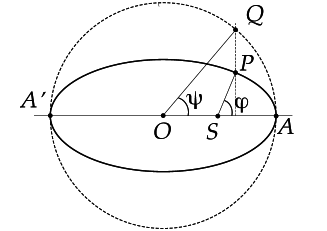
Figure 1: The geometry of Kepler’s Equation.

Suppose $P$ is the position of the planet at time $t$, which is measured by assuming the pericenter $A$ as the initial (i.e., at $t=0$) position (motion is counter-clockwise). Upon introducing the mean angular speed $\omega=2\pi/T$, with $T$ being the orbital period, the so-called mean anomaly, say $M$, is defined by $M=\omega t$. To retrieve the position of the planet along the orbit at time $t>0$, the angle $\psi$ is first evaluated by solving the following trascendental equation:

$$M\,=\,\psi\,-\,\epsilon\,\sin\,\psi\,,$$ (1)

which provides the position of point $Q$ along the circumscribed circle (dotted in the figure). The planet’s position $P$ is then immediately obtained through the geometrical construction sketched in Figure 1. Equation (1) is called the elliptic KE.

The Bessel solution of Equation (1) is provided by Colwell (1993) (Ch. 3)

$$\begin{array}[]{l}\displaystyle\psi\,=\,M\,+\,S(\epsilon;M)\,,\end{array}$$ (2)

where function $S(\epsilon;M)$ represents the Fourier series

$$\begin{array}[]{l}\displaystyle S(\epsilon;M)\,=\,\sum_{n=1}^{\infty}\,\frac{2\,J_{n}(n\,\epsilon)}{n}\,\sin\,nM\,.\end{array}$$ (3)

Although the series converges for any $\epsilon\in[0,1)$, its convergence turns out to be extremely slow, especially when $\epsilon\to 1$. This fact, together with the considerable number of Bessel function evaluations to be implemented, unavoidably resulted in Equations (2) and (3) being abandoned as far as the practical use of KE was concerned.

Nevertheless, the Bessel series expansion (3) remained a subject of considerable interest in both mathematics and theoretical physics. The scope of the present paper is to explore why this occurred. To this end, we introduce the complex function $\mathbb{S}(\epsilon;M)$, defined through the Kapteyn series

$$\begin{array}[]{l}\displaystyle\mathbb{S}(\epsilon;M)\,=\,\sum_{n=1}^{\infty}\,\frac{2\,J_{n}(n\,\epsilon)}{n}\,\exp(\mathrm{i}nM)\,,\end{array}$$ (4)

in such a way that $S=\mathrm{Im}\{\mathbb{S}\}$. The convergence of the series (4) can be proven, for example, by invoking the following Bessel function asymptotics, valid for $\epsilon<1$ Watson (1944) (Sec. 8.4):

$$\begin{array}[]{l}\displaystyle J_{n}(n\,\epsilon)\,\sim\,\frac{1}{\sqrt{2\pi\chi}}\,\frac{\exp(n\lambda)}{\sqrt{n}}\,,\qquad\quad n\to\infty\,,\end{array}$$ (5)

where $\chi=\sqrt{1-\epsilon^{2}}$ denotes the ellipse’s aspect ratio and $\lambda$ is a negative parameter, provided by

$$\begin{array}[]{l}\displaystyle\lambda=\chi\,+\,\dfrac{1}{2}\,\log\dfrac{1-\chi}{1+\chi}\,.\end{array}$$ (6)

The parameter $\lambda$ will play a key role in the rest of the paper.

After substituting Equation (5) into Equation (4) and upon introducing the complex parameter $z=\exp(\lambda+\mathrm{i}M)$, it can immediately be seen that the single terms of the series (4) asymptotically approach those of the paradigmatic model series

$$\begin{array}[]{l}\displaystyle\sum_{n=1}^{\infty}\,\frac{z^{n}}{n^{3/2}}\,,\end{array}$$ (7)

which, for $|z|<1$, is nothing but the Dirichlet series representation of the so-called polylogarithm function $\mathcal{L}_{3/2}(z)$, where

$$\begin{array}[]{l}\displaystyle\mathcal{L}_{\nu}(z)\,=\,\sum_{n=1}^{\infty}\,\frac{z^{n}}{n^{\nu}}\,,\qquad|z|<1\,.\end{array}$$ (8)

For $|z|\geq 1$, the series in Equation (8) can be analytically continuated to the whole complex plane, besides the half-axis $\mathrm{Re}\{z\}>1$.

More importantly (for the scopes of the present paper), functions $\mathcal{L}_{\nu}(z)$ are examples of Stieltjes function. For the reader’s convenience, the main definitions of Stieltjes functions and of Stieltjes series will now be briefly summarized. Interested readers can found some more useful references for instance in Ref. Caliceti et al. (2007). Moreover, the  formalism of Allen et al. Allen et al. (1975) will be adopted. Consider then an increasing real-valued function $\mu(t)$ defined for $t\in[0,\infty]$, with infinitely many points of increase. The measure $\mathrm{d}\mu$ is then positive on $[0,\infty]$. Assume all moments

$$\mu_{m}=\int_{0}^{\infty}\,t^{m}\,\mathrm{d}\mu\,,\qquad m\geq 0\,,$$ (9)

to be finite. Then, the formal power series

$$\sum_{m=0}^{\infty}\,\mu_{m}\,z^{m}\,,$$ (10)

is called a Stieltjes series. Such series turns out to be asymptotic, for  $z\to 0$, to the function $F(z)$ defined by

$$F(z)\,=\,\int_{0}^{\infty}\,\frac{\mathrm{d}\mu}{1-zt}\,,$$ (11)

which is called Stieltjes integral. To give a significative example, the Stieltjes nature of functions $\mathcal{L}_{\nu}$ will now be proved. To this end, it is sufficient to start from the following integral representation DLMF (25.12.11):

$$\begin{array}[]{l}\displaystyle\mathcal{L}_{\nu}(z)\,=\,-\dfrac{1}{\Gamma(\nu)}\,\int_{0}^{\infty}\,\dfrac{x^{\nu-1}\exp(-x)}{\exp(-x)-1/z\,}\,\mathrm{d}x,\end{array}$$ (12)

which, on setting $t=\exp(-x)$, gives

$$\begin{array}[]{l}\displaystyle\mathcal{L}_{\nu}(z)\,=\,z\,\int_{0}^{1}\,\dfrac{\left(-\log t\right)^{\nu-1}/{\Gamma(\nu)}}{1-zt}\,\mathrm{d}t\,,\end{array}$$ (13)

thus proving that the function $\mathcal{L}_{\nu}(z)/z$ is a Stieltjes integral exactly of the form (11), with the measure

$$\mu(t)\,=\,\left\{\begin{array}[]{lr}\displaystyle\dfrac{\Gamma(\nu,-\log t)}{\Gamma(\nu)}\,,&\qquad\qquad 0\leq t\leq 1,\\ &\\ 1&\qquad\qquad t>1\,,\end{array}\right.$$ (14)

where symbols $\Gamma(\cdot)$ and $\Gamma(\cdot,\cdot)$ denote the gamma and the incomplete gamma functions, respectively DLMF .

The above described “asymptotic connection” between series (4) and (7) via Equation (5) would at first sight suggest the function $\mathbb{S}(\epsilon;M)$ could be Stieltjes too. In the next section such a conjecture will definitely be proved.

III A Constructive Proof That $\mathbb{S}(\epsilon;M)$ Is a Stieltjes Series

We are now going to prove the following theorem: Function $\mathbb{S}(\epsilon;M)$ defined through the series (4) is a Stieltjes function.

First of all, the definition of $\mathbb{S}(\epsilon;M)$ given in Equation (4) must be recast as follows:

$$\begin{array}[]{l}\displaystyle\mathbb{S}(\epsilon;M)\,=\,\sum_{n=1}^{\infty}\,\frac{2\,J_{n}(n\,\epsilon)}{n}\exp(-\lambda n)\,z^{n}\,,\end{array}$$ (15)

with $z=\exp(\lambda+\mathrm{i}M)$. What we are going to show is that, similarly as for Equation (13), $\mathbb{S}$ can be written as

$$\begin{array}[]{l}\displaystyle\mathbb{S}(\epsilon;M)\,=\,z\int_{0}^{1}\,\dfrac{\rho(t)\,\mathrm{d}t}{1-zt}\,,\end{array}$$ (16)

where the measure $\mathrm{d}\mu=\rho(t)\mathrm{d}t$ represents the proof goal. Accordingly, the following infinite system must necessarily hold:

$$\begin{array}[]{l}\displaystyle\frac{2\,J_{n}(n\,\epsilon)}{n}\exp(-\lambda n)\,=\ \int_{0}^{1}\,t^{n-1}\,\rho(t)\,\mathrm{d}t\,,\qquad\qquad n\geq 1\,.\end{array}$$ (17)

The key tool of our proof is Watson’s integral representation of $J_{n}(n\epsilon)$, namely Watson (1917)

$$\begin{array}[]{l}\displaystyle J_{n}(n\,\epsilon)\,=\,\dfrac{1}{\pi}\,\int_{0}^{\pi}\,\exp[-n\,F(\theta;\epsilon)]\,\mathrm{d}\theta\,,\qquad\qquad 0\leq\epsilon\leq 1\,,\end{array}$$ (18)

where

$$\begin{array}[]{l}\displaystyle F(\theta;\epsilon)\,=\,\log\dfrac{\theta+\sqrt{\theta^{2}-\epsilon^{2}\sin^{2}\theta}}{\epsilon\,\sin\theta}\,-\,\dfrac{\sqrt{\theta^{2}-\epsilon^{2}\sin^{2}\theta}}{\tan\theta}\,,\qquad\theta\in[0,\pi]\,.\end{array}$$ (19)

Function $F(\theta;\epsilon)$ has features which reveal very important for our scopes. One of them is

$$\begin{array}[]{l}\displaystyle F\left(0;\sqrt{1-\chi^{2}}\right)\,+\,\lambda\,=\,0\,,\qquad\qquad 0\leq\chi\leq 1\,,\end{array}$$ (20)

which suggests Equation (18) to be recast as

$$\begin{array}[]{l}\displaystyle J_{n}(n\,\epsilon)\,\exp(-\lambda\,n)\,=\,\dfrac{1}{\pi}\,\int_{0}^{\pi}\,\exp[-n\,G_{\chi}(\theta)]\,\mathrm{d}\theta\,,\end{array}$$ (21)

where function $G_{\chi}(\theta)$ is defined as $G_{\chi}(\theta)=F\left(\theta;\sqrt{1-\chi^{2}}\right)+\lambda$.

Another property of $F(\theta;\epsilon)$ is that $\partial F(\theta;\epsilon)/\partial\theta>0$ for $\theta\in(0,\pi]$ Watson (1917). Then, in order for Equation (21) to be “tuned” with Equation (17), the new integration variable $t=\exp[-\,G_{\chi}(\theta)]$ is introduced, in such a way that

$$\begin{array}[]{l}\displaystyle\dfrac{\mathrm{d}t}{\mathrm{d}\theta}\,=\,-\exp[-\,G_{\chi}(\theta)]\dfrac{\mathrm{d}G_{\chi}(\theta)}{\mathrm{d}\theta}\,<\,0\,,\end{array}$$ (22)

for all values of $\theta$ except for $\theta=0$ and $\theta=\pi$, where $t^{\prime}(\theta)=0$. Accordingly, function $t=t(\theta)$ can be uniquely inverted into the function $\theta=\theta(t)$, formally defined by

$$\begin{array}[]{l}\displaystyle\theta(t)=F^{-1}[-\log t\,-\,\lambda]\,,\qquad\qquad t\in[0,1]\,,\end{array}$$ (23)

where the symbol $F^{-1}$ denotes the inverse of $F(\theta;\sqrt{1-\chi^{2}})$ with respect to $\theta$. Although its explicit analytical expression cannot be found, $\theta(t)$ can be easily numerically computed for any values of $t$ and $\chi$, for instance on using Mathematica’s native command InverseFunction. In Figure 2, the behaviour of $\theta(t)$, evaluated according to Equation (23), is plotted for different values of the aspect ratio $\chi$.

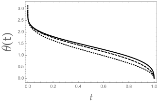
Figure 2: Behaviour of the function $\theta(t)$, according to Equation (23), for $\chi=1/10$ (solid curve), $\chi=1/2$ (dashed curve), and $\chi=1$ (dotted curve).

Now, we are going to prove that the function $\theta(t)$ actually coincides (apart some constant proportional factors), with the density $\rho(t)$ into Equation (16). To this end, it is sufficient to change the integration variable in Equation (21) from $\theta$ to $t$, which yields

$$\begin{array}[]{l}\displaystyle J_{n}(n\,\epsilon)\,\exp(-\lambda\,n)\,=\,-\dfrac{1}{\pi}\,\int_{0}^{1}t^{n}\,\theta^{\prime}(t)\,\mathrm{d}t\,.\end{array}$$ (24)

On performing the $t$-integration by parts we have

$$\begin{array}[]{l}\displaystyle J_{n}(n\,\epsilon)\,\exp(-\lambda\,n)\,=\,-\dfrac{1}{\pi}\,\left[t^{n}\,\theta(t)\right]_{0}^{1}\,+\,\dfrac{n}{\pi}\,\int_{0}^{1}t^{n-1}\,\theta(t)\mathrm{d}t\,=\,\dfrac{n}{\pi}\,\int_{0}^{1}t^{n-1}\,\theta(t)\mathrm{d}t\,,\end{array}$$ (25)

or, equivalently,

$$\begin{array}[]{l}\displaystyle\dfrac{2J_{n}(n\,\epsilon)\,\exp(-\lambda\,n)}{n}\,=\,\int_{0}^{1}\,t^{n-1}\,\dfrac{2\theta(t)}{\pi}\mathrm{d}t\,,\qquad\qquad n\geq 1\,,\end{array}$$ (26)

which, once compared to Equation (17), leads to $\rho(t)=2\theta(t)/\pi$.

The uniqueness of the function $\rho(t)$ can further be proved by invoking Calerman’s theorem for the Hausdorff problem, i.e., by showing that

$$\begin{array}[]{l}\displaystyle\sum_{m=0}^{\infty}\,\mu_{m}^{-1/{2m}}\,=\,+\infty\,.\end{array}$$ (27)

In order to prove the divergence of the above series, it is worth starting from the following inequality, proved by Siegel Siegel (1953):

$$\begin{array}[]{l}\displaystyle J_{n}(n\epsilon)\,\exp(-\lambda n)\,\leq 1\,,\qquad\qquad n\geq 1\,,\end{array}$$ (28)

according to which we have

$$\begin{array}[]{l}\displaystyle\dfrac{n}{J_{n}(n\epsilon)\,\exp(-\lambda n)}\,\geq n\,,\qquad\qquad n\geq 1\,,\end{array}$$ (29)

and then

$$\begin{array}[]{l}\displaystyle\lim_{n\to\infty}\left(\dfrac{n}{J_{n}(n\epsilon)\,\exp(-\lambda n)}\right)^{1/2n}\,\geq\lim_{n\to\infty}n^{1/2n}\,=\,1\,,\end{array}$$ (30)

which leads to Equation (27). Our proof is now complete. $\mathbb{S}(\epsilon;M)$ is a Stieltjes function.

IV A New Integral Representation of KE’s Solution

The proof given in Section III is the main result of the present paper. Here, an interesting byproduct of such proof is now illustrated. In particular, the “Stieltjesness” of $\mathbb{S}(\epsilon;M)$ will be employed to conceive a new, up to our knowledge, integral representation of the KE solution. To this end, Equation (16) is first recast as follows:

$$\begin{array}[]{l}\displaystyle\mathbb{S}(\epsilon;M)\,=\,-\dfrac{2}{\pi}\,\int_{0}^{1}\,\dfrac{\theta(t)}{t-1/z}\,\mathrm{d}t\,,\end{array}$$ (31)

so that formal partial integration gives

$$\begin{array}[]{l}\displaystyle\mathbb{S}(\epsilon;M)\,=\,-\dfrac{2}{\pi}\,\left[\theta(t)\,\log\left(t-\dfrac{1}{z}\right)\right]_{0}^{1}\,+\,\dfrac{2}{\pi}\,\int_{0}^{1}\,\log\left(t-\dfrac{1}{z}\right)\,\theta^{\prime}(t)\,\mathrm{d}t\,.\end{array}$$ (32)

The change of variable $t=\exp[-G_{\chi}(\theta)]$ then yields

$$\begin{array}[]{l}\displaystyle\mathbb{S}(\epsilon;M)\,=\,2\,\log\left(-\dfrac{1}{z}\right)\,\,-\,\dfrac{2}{\pi}\,\int_{0}^{\pi}\,\log\left(\exp[-G_{\chi}(\theta)]-\dfrac{1}{z}\right)\,\mathrm{d}\theta\,,\end{array}$$ (33)

which can be rearranged into a simpler form with a few work. First of all, we have

$$\begin{array}[]{l}\displaystyle\mathbb{S}(\epsilon;M)\,=\,2\,\log\left(-\dfrac{1}{z}\right)\,\,-\,\dfrac{2}{\pi}\,\int_{0}^{\pi}\,\log\left(\dfrac{z\,\exp[-G_{\chi}(\theta)]-1}{z}\right)\,\mathrm{d}\theta\,,\end{array}$$ (34)

or, equivalently,

$$\begin{array}[]{l}\displaystyle\mathbb{S}(\epsilon;M)\,=\,2\,\log\left(-\dfrac{1}{z}\right)\,\,-\,\dfrac{2}{\pi}\,\int_{0}^{\pi}\,\log\left(z\,\exp[-G_{\chi}(\theta)]-1\right)\,\mathrm{d}\theta\,-\,2\,\log\dfrac{1}{z}\,{=}\\ \\ \displaystyle\,{=}\,2\mathrm{i}\pi\,-\,\dfrac{2}{\pi}\,\int_{0}^{\pi}\,\log\left(\exp[-F(\theta;\epsilon)+\mathrm{i}M]-1\right)\,\mathrm{d}\theta\,.\end{array}$$ (35)

To retrieve the KE solution, it is sufficient to recall that $S(\epsilon;M)=\mathrm{Im}\{\mathbb{S}(\epsilon;M)\}$, which gives at once

$$\begin{array}[]{l}\displaystyle{S}(\epsilon;M)\,=\,2\pi\,+\,\dfrac{\mathrm{i}}{\pi}\,\int_{0}^{\pi}\,\mathrm{d}\theta\,\left\{\log\left(\exp[-F(\theta;\epsilon)+\mathrm{i}M]-1\right)\,\,-\,\log\left(\exp[-F(\theta;\epsilon)-\mathrm{i}M]-1\right)\right\}\,,\end{array}$$ (36)

that can also be recast as

$$\begin{array}[]{l}\displaystyle{S}(\epsilon;M)\,=\,\dfrac{\mathrm{i}}{\pi}\,\int_{0}^{\pi}\,\log\dfrac{1\,-\,\exp[-\,F(\theta;\epsilon)\,+\,\mathrm{i}M]}{1\,-\,\exp[-\,F(\theta;\epsilon)\,-\,\mathrm{i}M]}\,\mathrm{d}\theta\,,\end{array}$$ (37)

where the term $2\pi$ in Equation (36) must be removed, due to the phase wrapping of the principal branch of the natural logarithm, $-\pi<\arg\{\log z\}\leq\pi$.

Equation (37) is the other main result of the present paper. Compared with other, formally similar integral representations of the KE solution, for instance that in Eisinberg et al. (2010), Equation (37) is expected to provide computational advantages due to the monotonic decreasing behaviour of the function $\exp[-F(\theta;\epsilon)]$ within the integration interval $\theta\in[0,\pi]$.

Just to provide an idea, a single but significant numerical experiment will now be carried out by using only native commands of Mathematica. A case of particular interest is that of nearly parabolic orbits around the periapsis, which correspond to $\epsilon\to 1$. Accurate numerical solutions for such a critical regime can be found, for instance, in Tommasini (2022); Farnocchia (2013). In particular, in Farnocchia (2013), it was emphasized how solving the elliptic KE for a given couple $(\epsilon,M)$ resulted in a bad conditioned problem in the neighbourhood of $(1,0)$. To provide an example of the computational use of the new integral representation in Equation (37), we considered the sole case of a parabolic orbit, i.e.,  $\epsilon=1$.

In Figure 3, the relative error, evaluated with respect to the “exact KE solution”, is plotted against $M\in(0,\pi)$. In the above experiments, such an “exact value” was evaluated by solving Equation (1) via Mathematica’s native command FindRoot with the parameter WorkingPrecision set to 50 and an initial guess of $\psi=\pi$. Function $S(\epsilon;M)$ was evaluated by implementing Equation (36) using the native Mathematica command NIntegrate with different degrees of accuracy, measured by the parameter WorkingPrecision, which was set to 10 (a), 15 (b), 20 (c), and  25 (d).

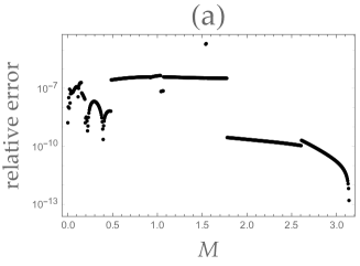
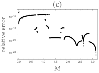
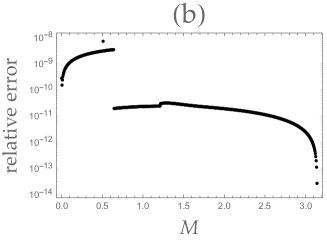
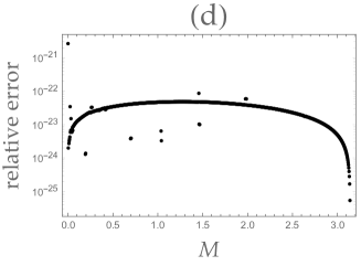
Figure 3: Behaviour of the relative error against $M\in(0,\pi)$. In the above experiments, the “exact value” of the KE solution was evaluated by solving Equation (1) via Mathematica’s native command FindRoot with the parameter WorkingPrecision set to 50 and the initial guess of $\psi=\pi$. Function $S(\epsilon;M)$ was evaluated by implementing Equation (36) through the native Mathematica command NIntegrate with different degrees of accuracy, measured by the parameter WorkingPrecision, which was set to 10 (a), 15 (b), 20 (c), and  25 (d).

V Discussions

Here, the classical Bessel solution of Kepler’s equation was revisited from a new perspective, offered by the beautiful theory of the Stieltjes series. In particular, after introducing a “complexified” version of the original Kapteyn series (3), its Stieltjes nature was mathematically proven. Our principal tool was Watson’s integral representation of Bessel functions. As a potentially interesting by-product of our analysis, to our knowledge, a new integral representation of the KE solution was achieved.

Exploring the Stieltjes nature of Equation (4) could also reveal new interesting aspects concerning the more general framework of the Kapteyn series. The need to develop new methods to achieve the summability of the Kapteyn series of both the first and second kind have already been invoked in the recent past Tautz et al. (2011). In this respect, we believe the results presented here could be of some help.

Just to gain an idea, consider again the Kapteyn series $\displaystyle\sum_{m\geq 1}\,\dfrac{z^{m}}{m}\,J_{m}(m\epsilon)$, but suppose that $|z|>\exp(-\lambda)$. In that case, the series diverges. However, the analysis carried out in Section III is also still valid for $z$ belonging to the whole complex plane, provided that $|\mathrm{arg}(z)|<\pi$. In other words, our Kapteyn series can be continued to a Stieltjes function according to

$$\begin{array}[]{l}\displaystyle\displaystyle\sum_{m\geq 1}\,\dfrac{z^{m}}{m}\,J_{m}(m\epsilon)\,\sim\,\mathrm{i}\pi\,-\,\dfrac{1}{\pi}\,\int_{0}^{\pi}\,\log\left(z\,\exp[-F(\theta;\epsilon)]-1\right)\,\mathrm{d}\theta\,,\quad|\mathrm{arg}(z)|<\pi\,.\end{array}$$ (38)

which lives, for $\epsilon\in[0,1)$, on the whole complex plane, besides the infinite interval $(1,\infty)$.

Proving that a divergent power series is a Stieltjes series also implies that such a series would be Padé summable. To quote an important example, in Bender and Weniger (2001), numerical evidence for the factorially divergent perturbation expansion for energy eigenvalues of the PT-symmetric Hamiltonian $H(\lambda)=p^{2}+1/4x^{2}+\mathrm{i}\lambda x^{3}$ being a Stieltjes series and thus Padé summable, were provided. Such conjecture was later rigorously proven in Grecchi et al. (2009). The Padé summability of our Kapteyn series also implies that suitable resummation algorithms, the most well-known being Wynn’s $\epsilon$ algorithm, can successfully be employed to retrieve the correct value provided in Equation (38). Padé approximants remain the most favourite mathematical tool to resume divergent and slowly convergent series in theoretical physics. This is because a solid convergence theory has been established for them, especially in the case of Stieltjes asymptotic series Bender and Orszag (1978); Baker and Graves-Morris (1996); Widder (1938). In particular, if the input data are the partial sums of a Stieltjes series, it can be rigorously proven that certain subsequences of the Padé table converge to the value of the corresponding Stieltjes function Baker and Graves-Morris (1996); Brezinski (1996) (Chapter 5). A typical feature of Wynn’s $\epsilon$ algorithm is that only the input of the numerical values of a finite substring of the partial sequence of the series is required to achieve a meaningful resummation.

In the case of the Stieltjes series, however, important additional structural information about the behaviour of the series terms is available. For example, it is known that the magnitudes of the truncation errors are bounded by the first term neglected in the partial sum, and they also have the same sign patterns. In the seminal 1973 paper by Levin Levin (1973), a new class of sequence transformations was introduced that used such valuable a priori structural information to improve the efficiency and convergence speed of the transformed sequences. For a general discussion on the construction principles of Levin-type sequence transformations, readers are encouraged to go through the paper by Weniger Weniger (1989), as well as through Ref. Borghi and Weniger (2015), which contains a slightly upgraded and formally improved version of the former. To provide a simple example, Table 1 shows the performance of a particular Levin-type transformation, the so-called Weniger $\delta$-transformation Weniger (1989), in the resummation of the Kapteyn series on the left side of Equation (38) for $\epsilon=9/10$ and $z=10\,\exp(\mathrm{i}\pi/3)$.

The convergence to the value obtained by numerically computing the integral on the right side of Equation (38) is evident.

order Partial sum sequence Weniger $\delta$-transformation 1 2.02+3.51 i 0.112240 + 1.211289 i 10 (4.4 - 10. i) $\times 10^{8}$ -1.003096 +1.238166 i 20 (-3.1 + 32. i) $\times 10^{18}$ -1.001839 + 1.238763 i 30 (7.7 +10. i) $\times 10^{27}$ -1.001838 + 1.238765 i … … …

Table 1: Resummation, via Weniger $\delta$-transformation Weniger (1989), of the (divergent) Kapteyn series $\displaystyle\sum_{m\geq 1}\,\dfrac{z^{m}}{m}\,J_{m}(m\epsilon)$, evaluated for $z=10\,\exp(\mathrm{i}\pi/3)$. The value obtained by numerically computing the integral into the right side of Equation (38) is: $-$1.001838…+ 1.238765…i.

Finally, before concluding, it is worth illustrating at least one experiment of the use of the Weniger transformation to solve Kepler’s equation. Once again, the parabolic case will be analysed, but now only “small values” of $M$, namely less than $1/10$, will be considered. In Figure 4, the relative error is still plotted versus $M\in\left[\dfrac{1}{1000},\dfrac{1}{10}\right]$. Again, the “exact solution” was evaluated by solving Equation (1) via Mathematica’s command FindRoot with the parameter WorkingPrecision set to 50 and an initial guess of $\psi=\pi$, but now the function $S(\epsilon;M)$ is thought of as the imaginary part of $\mathbb{S}(\epsilon;M)$. The latter is computed, as done in Table 1, via the Weniger $\delta$-transformation with different orders.

Figure 4: The same as in Figure 3, but for $M\in\left[\dfrac{1}{1000},\dfrac{1}{10}\right]$. Note that now the function $S(\epsilon;M)$ is thought of as the imaginary part of $\mathbb{S}(\epsilon;M)$, which is computed, similarly to that in Table 1, via the Weniger $\delta$-transformation with an order of 20 (black circles), 30 (open circles), 40 (open squares), and 50 (black squares).

VI Conclusions

In common with almost any scientific problem which achieves a certain longevity and whose literature exceeds a certain critical mass, the Kepler problem has acquired luster and allure for the modern practitioner. Any new technique for the treatment of trascendental equations should be applied to this illustrious case; any new insight, however slight, lets its conceiver join an eminent list of contributors.

Nothing can illustrate the fascination that Kepler’s equation has held for nearly 400 years better than the above paragraph, which appears in the introduction to Colwell’s book. Kepler’s problem continues to inspire mathematicians, scientists, and engineers to search for further contributions to the subject. In the present paper, the Bessel solution of KE has been studied from the perspective of Stieltjes function theory. In particular, it has been proven that the Kapteyn series (3) obtained by the “complexification” of the Bessel series solution (2) is a Stieltjes series. Moreover, thanks to our constructive proof, to our knowledge, a new integral representation of the KE solution has been obtained. More importantly, the limit of validity of such a representation extends far beyond that fixed by the convergence circle of the Kapteyn series itself.

Stieltjes series are strictly connected with Padé summability via a well established convergence theory. Divergent Stieltjes series can be resummed to the corresponding Stieltjes integral values using Padé approximants. In the last 40 years, Levin-type transformations have been shown to possess retrieving capabilities considerably superior to those of Padé, as far as the resummation of the Stieltjes series is concerned. At present, the main theoretical drawback of Levin-type transformations is the lack of a rigorous convergence theory, like that available for Padé. Thus, we also hope that what is contained in the present paper could provide a further contribution to the construction of such a convergence theory, also in order to provide Levin-type transformations the scientific recognition they certainly deserve, but that, unfortunately, in our opinion, still seems too far away.

References

- Colwell (1993) Colwell, P. Solving Kepler’s Equation Over Three Centuries; Willmann-Bell: Richmond, VA, USA, 1993.
- Ibrahim and Saleh (2019) Ibrahim, R.; Saleh, A.R. Re-evaluation solution methods for Kepler’s equation of an elliptical orbit. Iraqi J. Sci. 2019, 60, 2269–2279.
- Calvo et al. (2019) Calvo, M.; Elipe, A.; Montijano, J.; Rández, L. A monotonic starter for solving the hyperbolic Kepler equation by Newton method. Celest. Mech. Dyn. Astron. 2019, 131, 18.
- Tommasini and Olivieri (2020) Tommasini, D.; Olivieri, D. Fast switch and spline scheme for accurate inversion of nonlinear functions: The new first choice solution to Kepler’s equation. Appl. Math. Comput. 2020, 364, 124677.
- Abubekerov and Gostev (2020) Abubekerov, M.K.; Gostev, N.Y. Solution of Kepler’s Equation with Machine Precision. Astron. Rep. 2020, 64, 1060–1066.
- Sacchetti (2020) Sacchetti, A. Francesco Carlini: Kepler’s equation and the asymptotic solution to singular differential equations. Hist. Math. 2020, 53, 1–32.
- Tommasini and Olivieri (2020) Tommasini, D.; Olivieri, D. Fast Switch and Spline Function Inversion Algorithm with Multistep Optimization and k-Vector Search for Solving Kepler’s Equation in Celestial Mechanics. Mathematics 2020, 8, 2017.
- Zechmeister (2021) Zechmeister, M. Solving Kepler’ss equation with CORDIC double iterations. Mon. Not. R. Astron. Soc. 2021, 500, 109–117.
- González-Gaxiola and Hernández-Linares (2021) González-Gaxiola, O.; Hernández-Linares, S. An Efficient Iterative Method for Solving the Elliptical Kepler’s Equation. Int. J. Appl. Comput. Math. 2021, 7, 42.
- Tommasini (2021) Tommasini, D. Bivariate Infinite Series Solution of Kepler’s Equation. Mathematics 2021, 9, 785.
- Philcox et al. (2021) Philcox, O.H.E.; Goodman, J.; Slepian, Z. Kepler’s Goat Herd: An exact solution to Kepler’s equation for elliptical orbits. Mon. Not. R. Astron. Soc. 2021, 506, 6111–6116.
- Tommasini (2022) Tommasini, D.; Olivieri, D. Two fast and accurate routines for solving the elliptic Kepler equation for all values of the eccentricity and mean anomaly. Astron. Astrophys. 2022, 658, A196.
- Zhang et al. (2022) Zhang, R.; Bian, S.; Li, H. Symbolic iteration method based on computer algebra analysis for Kepler’s equation. Sci. Rep. 2022, 12, 2957.
- Wu et al. (2023) Wu, B.; Zhou, Y.; Lim, C.W.; Zhong, H. A new solution approach via analytical approximation of the elliptic Kepler equation. Acta Astronaut. 2023, 202, 303–310.
- Vavrukh et al. (2023) Vavrukh, M.; Dzikovskyi, D.; Stelmakh, O. Analytical images of Kepler’s equation solutions and their applications. Math. Model. Comput. 2023, 10, 351–358.
- Calvo et al. (2023) Calvo, M.; Elipe, A.; Rández, L. On the integral solution of elliptic Kepler’s equation. Celest. Mech. Dyn. Astron. 2023, 135, 26.
- Brown (2023) Brown, M.T. An improved cubic approximation for K epler’s equation. Mon. Not. R. Astron. Soc. 2023, 525, 57–66.
- Kapteyn (1893) Kapteyn, W. Researches sur les functions de Fourier-Bessel. Ann. Sci. L’Ecole Norm. Sup. Ser. 1893, 3, 91–122.
- Dominici (2007) Dominici, D. A new Kapteyn series. Integral Transform. Spec. Funct. 2007, 18, 409–418.
- Lerche and Tautz (2007) Lerche, I.; Tautz, R. A note on summation of kapteyn series in astrophysical problems. Astrophys. J. 2007, 665, 1288–1291.
- Pogány (2007) Pogány, T.K. Convergence of generalized Kapteyn expansion. Appl. Math. Comput. 2007, 190, 1844–1847.
- Lerche and Tautz (2008) Lerche, I.; Tautz, R. Kapteyn series arising in radiation problems. J. Phys. A Math. Theor. 2008, 41, 035202.
- Lerche et al. (2009) Lerche, I.; Tautz, R.; Citrin, D. Terahertz-sideband spectra involving Kapteyn series. J. Phys. A Math. Theor. 2009, 42, 365206.
- Eisinberg et al. (2010) Eisinberg, A.; Fedele, G.; Ferrise, A.; Frascino, D. On an integral representation of a class of Kapteyn (Fourier-Bessel) series: Kepler’s equation, radiation problems and Meissel’s expansion. Appl. Math. Lett. 2010, 23, 1331–1335.
- Tautz et al. (2011) Tautz, R.C.; Lerche, I.; Dominici, D. Methods for summing general Kapteyn series. J. Phys. A Math. Theor. 2011, 44, 385202.
- Baricz et al. (2011) Baricz, A.; Jankov, D.; Pogány, T.K. Integral representation of first kind Kapteyn series. J. Math. Phys. 2011, 52, 043518.
- Nikishov (2014) Nikishov, A.I. Kapteyn series and photon emission. Bull. Lebedev Phys. Inst. 2014, 41, 332–338.
- Baricz et al. (2017) Baricz, A.; Masirevic, D.J.; Pogány, T.K. Kapteyn Series. Lect. Notes Math. 2017, 2207, 87–111.
- Xue et al. (2019) Xue, X.; Li, Z.; Man, Y.; Xing, S.; Liu, Y.; Li, B.; Wu, Q. Improved Massive MIMO RZF Precoding Algorithm Based on Truncated Kapteyn Series Expansion. Information 2019, 10, 136.
- Bornemann (2023) Bornemann, F. A Jentzsch-Theorem for Kapteyn, Neumann and General Dirichlet Series. Comput. Methods Funct. Theory 2023, 23, 723–739.
- Bender and Orszag (1978) Bender, C.M.; Orszag, S.A. Advanced Mathematical Methods for Scientists and Engineers; McGraw-Hill: New York, NY, USA, 1978.
- Baker and Graves-Morris (1996) Baker, Jr., G.A.; Graves-Morris, P. Padé Approximants, 2nd ed.; Cambridge U. P.: Cambridge, UK, 1996.
- Widder (1938) Widder, D.V. The Stieltjes transform. Trans. Am. Math. Soc. 1938, 43, 7–60.
- Brezinski (1996) Brezinski, C. Extrapolation algorithms and Padé approximations: A historical survey. Appl. Numer. Math. 1996, 20, 299–318.
- Orlando et al. (2018) Orlando, F.; Farina, C.; Zarro, C.; Terra, P. Kepler’s equation and some of its pearls. Am. J. Phys. 2018, 86, 11.
- Watson (1944) Watson, G.N. A Treatise on the Theory of Bessel Functions; Cambridge University Press: Cambridge, UK, 1944.
- Caliceti et al. (2007) Caliceti, E.; Meyer-Hermann, M.; Ribeca, P.; Surzhykov, A.; Jentschura, U.D. From useful algorithms for slowly convergent series to physical predictions based on divergent perturbative expansions. Phys. Rep. 2007, 446, 1–96.
- Allen et al. (1975) Allen, G.D.; Chui, C.K.; Madych, W.R.; Narcowich, F.J.; Smith, P.W. Padé approximation of Stieltjes series. J. Approx. Theory 1975, 14, 302–316.
- (39) Olver, F.W.J.; Olde Daalhuis, A.B.; Lozier, D.W.; Schneider, B.I.; Boisvert, R.F.; Clark, C.W.; Miller, B.R.; Saunders, B.V.; Cohl, H.S.; McClain, M.A. (eds.) NIST Digital Library of Mathematical Functions. Release 1.1.3 of 2021-09-15. 2022. Available online: http://dlmf.nist.gov/
- Watson (1917) Watson, G.N. Bessel functions and Kapteyn series. Proc. Lond. Math. Soc. 1917, 16, 150–174.
- Siegel (1953) Siegel, K.M. An inequality involving Bessel functions of argument nearly equal to their order. Proc. Am. Math. Soc. 1953, 4, 858–859.
- Farnocchia (2013) Farnocchia, D.; Cioci, D.B.; Milani, A. Robust resolution of Kepler’s equation in all eccentricity regimes. Celest. Mech. Dyn. Astron. 2013, 116, 21–34.
- Bender and Weniger (2001) Bender, C.M.; Weniger, E.J. Numerical evidence that the perturbation expansion for a non-Hermitian -symmetric Hamiltonian is Stieltjes. J. Math. Phys. 2001, 42, 2167–2183.
- Grecchi et al. (2009) Grecchi, V.; Maioli, M.; Martinez, A. Padé summability of the cubic oscillator. J. Phys. A 2009, 42, 425208.
- Levin (1973) Levin, D. Development of non-linear transformations for improving convergence of sequences. Int. J. Comput. Math. B 1973, 3, 371–388.
- Weniger (1989) Weniger, E.J. Nonlinear sequence transformations for the acceleration of convergence and the summation of divergent series. Comput. Phys. Rep. 1989, 10, 189–371.
- Borghi and Weniger (2015) Borghi, R.; Weniger, E.J. Convergence analysis of the summation of the factorially divergent Euler series by Padé approximants and the delta transformation. Appl. Numer. Math. 2015, 94, 149–178.