Productions of $D^{*}_{s0}(2317)$ and $D_{s1}(2460)$ in $B_{(s)}$ and $\Lambda_{b}(\Xi_{b})$ decays

Abstract

Recent studies show that $D_{s0}^{\ast}(2317)$ and $D_{s1}(2460)$ contain large molecular components. In this work, we employ the naive factorization approach to calculate the production rates of $D_{s0}^{\ast}(2317)$ and $D_{s1}(2460)$ as hadronic molecules in $B_{(s)}$ and $\Lambda_{b}(\Xi_{b})$ decays, where their decay constants are estimated in the effective Lagrangian approach. With the so-obtained decay constants $f_{D_{s0}^{\ast}(2317)}$ and $f_{D_{s1}(2460)}$, we calculate the branching fractions of the $b$-meson decays $B_{(s)}\to\bar{D}_{(s)}^{(*)}D_{s0}^{*}$ and $B_{(s)}\to\bar{D}_{(s)}^{(*)}D_{s1}$ and the $b$-baryon decays $\Lambda_{b}(\Xi_{b})\to\Lambda_{c}(\Xi_{c})D_{s0}^{*}$ and $\Lambda_{b}(\Xi_{b})\to\Lambda_{c}(\Xi_{c})D_{s1}$. Our results show that the production rates of $D_{s0}^{\ast}(2317)$ and $D_{s1}(2460)$ in the $B_{s}$, $\Lambda_{b}$ and $\Xi_{b}$ decays are rather large that future experiments could observe them. In particular, we demonstrate that one can extract the decay constants of hadronic molecules via the triangle mechanism because of the equivalence of the triangle mechanism to the tree diagram established in calculating the decays $B\to\bar{D}^{(*)}D_{s0}^{\ast}(2317)$ and $B\to\bar{D}^{(*)}D_{s1}(2460)$.

I Introduction

In 2003, the BarBar Collaboration discovered $D_{s0}^{*}(2317)$ in the $D_{s}^{+}\pi^{0}$ mass distribution in the $e^{+}e^{-}$ annihilation process Aubert et al. (2003), which was later confirmed by the CLEO Collaboration Besson et al. (2003) and Belle Collaboration Mikami et al. (2004) in the same process. Moreover, the BESIII Collaboration observed the $D_{s0}^{*}(2317)$ in the process of $e^{+}e^{-}\to D_{s}^{*+}D_{s0}^{*-}(2317)$ Ablikim et al. (2018). In addition to the above inclusive processes, $D_{s0}^{*}(2317)$ was also observed in the exclusive process of the $B$ decay by the Belle Collaboration Krokovny et al. (2003) and BarBar Collaboration Aubert et al. (2004a). $D_{s1}(2460)$ as the heavy quark spin symmetry (HQSS) partner of $D_{s0}^{*}(2317)$ was first discovered in the $D_{s}^{\ast+}\pi^{0}$ mass distribution by the CLEO Collaboration Besson et al. (2003), and then confirmed by several other experiments Mikami et al. (2004); Krokovny et al. (2003); Aubert et al. (2004b). Treating $D_{s0}^{*}(2317)$ and $D_{s1}(2460)$ as conventional $P$-wave $c\bar{s}$ mesons, the masses obtained in the Goldfrey-Isgur (GI) model are larger than the experimental ones by 140 MeV and 100 MeV Godfrey and Isgur (1985), which have motivated extensive discussions on their nature.

By analyzing their masses, several interpretations were proposed for the internal structure of $D_{s0}^{*}(2317)$ and $D_{s1}(2460)$. In Ref. Song et al. (2015), the authors found that the masses of $D_{s0}^{*}(2317)$ and $D_{s1}(2460)$ still deviate from the experimental data, even adding the screen potential to the conventional quark model. However, as the $DK$ and $D^{*}K$ components were embodied into the conventional quark model, the mass puzzle of $D_{s0}^{*}(2317)$ and $D_{s1}(2460)$ is resolved Albaladejo et al. (2018); Yang et al. (2022); Luo et al. (2021), which indicates that the $D^{(*)}K$ components play an important role in forming $D_{s0}^{*}(2317)$ and $D_{s1}(2460)$. Therefore, $D_{s0}^{*}(2317)$ and $D_{s1}(2460)$ are proposed to be hadronic molecules of $DK$ and $D^{*}K$ to explain their masses, especially their mass splitting Barnes et al. (2003); Gamermann et al. (2007); Guo et al. (2006); Xie et al. (2010); Cleven et al. (2011); Guo et al. (2015); Wu et al. (2019). It should be noted that in the lattice QCD simulation of the $DK$ interaction, a bound state below the $DK$ mass threshold was identified Liu et al. (2013); Mohler et al. (2013); Lang et al. (2014); Bali et al. (2017); Alexandrou et al. (2020). Furthermore, with the $D^{(*)}K$ potentials supplemented by the $c\bar{s}$ core couplings to the $D^{(*)}K$ components, $D_{s0}^{*}(2317)$ and $D_{s1}(2460)$ can be dynamically generated Weinberg (1965); Martínez Torres et al. (2015); Albaladejo et al. (2016); Song et al. (2022), indicating that the $D^{(*)}K$ molecular components account for a large proportion of their wave functions in terms of the Weinberg compositeness rule $1-Z$ Weinberg (1965). Studying the masses of $D_{s0}^{*}(2317)$ and $D_{s1}(2460)$, one can conclude that they contain both $D^{(*)}K$ molecular components and a $c\bar{s}$ core. The natural next step forward is to study their decays.

According to the review of particle physics (RPP) Workman et al. (2022), the $D_{s0}^{*}(2317)^{+}$ dominantly decays to $D_{s}^{+}\pi^{0}$, which means that $D_{s0}^{*}(2317)^{+}$ must be narrow since the decay of $D_{s0}^{*}(2317)^{+}\to D_{s}^{+}\pi^{0}$ breaks isospin. The dominant decay of $D_{s1}(2460)$ into $D_{s}^{*+}\pi^{0}$ and $D_{s}^{+}\gamma$ is responsible for its narrow width. The narrow widths of $D_{s0}^{*}(2317)$ and $D_{s1}(2460)$ are quite different from the widths of their SU(3)-flavor partners $D^{*}_{0}(2300)$ and $D_{1}(2430)$, which reflects the exotic properties of these excited charmed mesons. In Refs. Fayyazuddin and Riazuddin (2004); Ishida et al. (2004); Wei et al. (2006); Nielsen (2006); Song et al. (2015), the authors proposed that the decays of $D_{s0}^{*}(2317)$ and $D_{s1}(2460)$ as the $c\bar{s}$ excited states into $D_{s}\pi$ and $D_{s}^{*}\pi$ proceed via the $\pi-\eta$ mixing, resulting in widths of tens of keV. Treating $D_{s0}^{*}(2317)$ and $D_{s1}(2460)$ as hadronic molecules, their widths are of the order of $100$ keV Faessler et al. (2007a, b); Fu et al. (2022). Up to now, there are no precise experimental measurements of the widths of $D_{s0}^{*}(2317)$ and $D_{s1}(2460)$, but only their upper limits of $3.8$ MeV. From the perspective of their widths, one can obtain the same conclusion as from the studies of their masses regarding the nature of $D_{s0}^{*}(2317)$ and $D_{s1}(2460)$. It is worth noting that a model-independent method has been proposed to verify the molecular nature of $D_{s0}^{*}(2317)$ by experimental searches for its three-body counterparts $DDK$ and $D\bar{D}K$ Wu et al. (2019); Huang et al. (2020); Wu et al. (2022); Wu and Geng (2023).

The discoveries of $D_{s0}^{*}(2317)$ and $D_{s1}(2460)$ in the inclusive and exclusive processes in $e^{+}e^{-}$ collisions triggered a series of theoretical works to investigate their production mechanism. Assuming $D_{s0}^{*}(2317)$ and $D_{s1}(2460)$ as $D^{(*)}K$ hadronic molecules and $c\bar{s}$ excited states, Wu et al. estimated that their production rates in $e^{+}e^{-}$ collisions are of the order of $10^{-3}$ Wu and Geng (2023), consistent with the experimental data Aubert et al. (2006). As for the exclusive process, Faessler et al. calculated the decays $B\to D_{s0}^{*}(2317)\bar{D}^{(*)}$ and $B\to D_{s1}(2460)\bar{D}^{(*)}$ assuming $D_{s0}^{*}(2317)$ and $D_{s1}(2460)$ as $D^{(*)}K$ molecules Faessler et al. (2007c). The results are a bit smaller than the experimental data. Assuming $D_{s0}^{*}(2317)$ and $D_{s1}(2460)$ as $c\bar{s}$ excited states, the decays $B\to D_{s0}^{*}(2317)\bar{D}^{(*)}$ and $B\to D_{s1}(2460)\bar{D}^{(*)}$ were investigated as well, but the results suffer from large uncertainties Colangelo et al. (1991); Veseli and Dunietz (1996); Cheng et al. (2004); Colangelo et al. (2005); Cheng and Chua (2006); Segovia et al. (2012). Moreover, the productions of $D_{s0}^{*}(2317)$ and $D_{s1}(2460)$ in the $\Lambda_{b}$ decays have been explored Datta et al. (2004), finding that their production rates in the $\Lambda_{b}$ decays are larger than those in the corresponding $B$ decays. Recently, the $DK$ femtoscopic correlation function was investigated to elucidate the nature of $D_{s0}^{*}(2317)$ Liu et al. (2023); Ikeno et al. (2023), which can be accessed in high energy nucleon-nucleon collisions in the future Adamczyk et al. (2015); Collaboration et al. (2020).

Until now, the $D_{s0}^{*}(2317)$ and $D_{s1}(2460)$ have only been observed in the exclusive process via $B$ decays. In this work, we systematically explore the productions of $D_{s0}^{*}(2317)$ and $D_{s1}(2460)$ in $B_{(s)}$ and $\Lambda_{b}(\Xi_{b})$ decays with the factorization ansatz Chau (1983); Chau and Cheng (1987). Following Ref. Faessler et al. (2007c), we employ the effective Lagrangian approach to estimate the decay constants of ${D_{s0}^{*}(2317)}$ and ${D_{s1}(2460)}$, which are dynamically generated via the $DK-D_{s}\eta$ and $D^{*}K-D_{s}^{*}\eta$ coupled-channel potentials described by the contact-range effective field theory (EFT), and then calculate the production rates of $D_{s0}^{*}(2317)$ and $D_{s1}(2460)$ in $B_{(s)}$ and $\Lambda_{b}(\Xi_{b})$ decays. Another motivation of this work is to test the universality of the approach that we proposed to calculate the decay constant of a hadronic molecule via the triangle mechanism Wu et al. (2023). Based on our previous study of the decays $B\to D_{s0}^{*}(2317)\bar{D}^{(*)}$ and $B\to D_{s1}(2460)\bar{D}^{(*)}$ via the triangle mechanism, the decay constants of $D_{s0}^{*}(2317)$ and $D_{s1}(2460)$ can be extracted Liu et al. (2022). The effective Lagrangian approach in this work can further check the validity of our approachWu et al. (2023).

This paper is organized as follows. In Sec. II, we introduce the effective Lagrangian approach to calculate the productions of $D_{s0}^{*}(2317)$ and $D_{s1}(2460)$ in $B_{(s)}$ and $\Lambda_{b}(\Xi_{b})$ decays and the decay constants of $f_{D_{s0}^{*}}$ and $f_{D_{s1}}$. Results and discussions are given in Sec. III, followed by a summary in Sec. IV.

II Theoretical formalism

II.1 Effective Lagrangians for nonleptonic Weak decays

In this work, we focus on the productions of $D_{s0}^{*}(2317)$ and $D_{s1}(2460)$ in $B_{(s)}$ and $\Lambda_{b}(\Xi_{b})$ decays. At quark level, the Cabibbo-favored decays $B^{+}\to\bar{D}^{(\ast)0}D_{s}^{(\ast)+}$ and $\Lambda_{b}\to\Lambda_{c}D_{s}^{(\ast)+}$ mainly proceed via the external $W$-emission mechanism shown in Fig. 1 according to the topological classification of weak decays Chau and Cheng (1987); Ali et al. (1998, 2007); Li et al. (2012), which the naive factorization approach can well describe. With the factorization ansatz Bauer et al. (1987), the amplitudes of the weak decays $B^{+}\to\bar{D}^{(\ast)0}D_{s}^{(\ast)+}$ and $\Lambda_{b}\to\Lambda_{c}D_{s}^{(\ast)+}$ can be expressed as products of two current matrix elements

$$\mathcal{A}\left(B^{+}\to D_{s}^{(\ast)+}\bar{D}^{(\ast)0}\right) = \frac{G_{F}}{\sqrt{2}}V_{cb}V_{cs}a_{1}\left\langle D_{s}^{(\ast)+}|(s\bar{c})|0\right\rangle\left\langle\bar{D}^{(\ast)0}|(c\bar{b})|B^{+}\right\rangle,$$ (1)

$$\mathcal{A}\left(\Lambda_{b}\to D_{s}^{(\ast)+}\Lambda_{c}\right) = \frac{G_{F}}{\sqrt{2}}V_{cb}V_{cs}a_{1}\left\langle D_{s}^{(\ast)+}|(s\bar{c})|0\right\rangle\left\langle\Lambda_{c}|(c\bar{b})|\Lambda_{b}\right\rangle,$$ (2)

where $G_{F}$ is the Fermi constant, $V_{cb}$ and $V_{cs}$ are the Cabibbo-Kobayashi-Maskawa (CKM) matrix elements, and $a_{1}$ is the effective Wilson coefficient. In principle, $a_{1}$ is expressed by the Wilson Coefficients of the QCD-corrected effective weak Hamiltonian, which depends on the renormalization scale Chau and Cheng (1987); Cheng and Tseng (1993); Cheng and Chiang (2010). In this work, we parameterize the non-factorization contributions with the effective Wilson coefficient $a_{1}$, which can be determined by reproducing relevant experimental data.

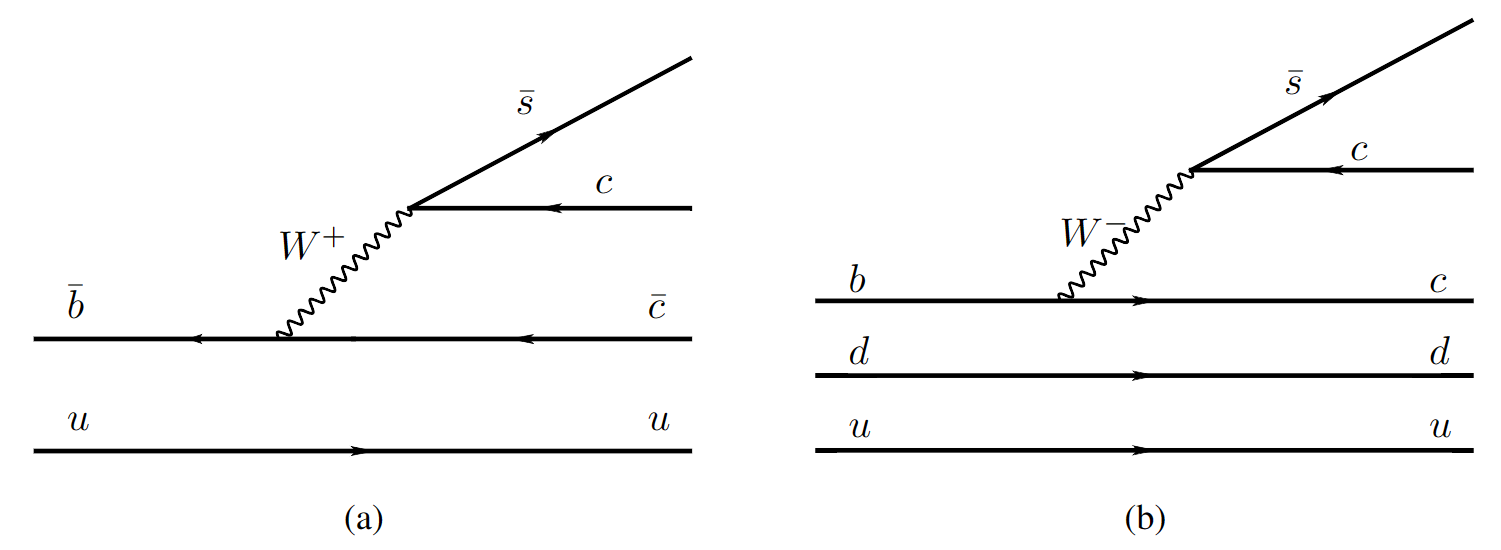
Figure 1: External $W$-emission mechanism for $B^{+}\to\bar{D}^{(\ast)0}D_{s}^{(\ast)+}$ (a) and $\Lambda_{b}\to\Lambda_{c}D_{s}^{(\ast)+}$ (b).

The current matrix elements of $\left\langle\bar{D}^{0}|(c\bar{b})|B^{+}\right\rangle$ and $\left\langle\bar{D}^{\ast 0}|(c\bar{b})|B^{+}\right\rangle$ describing the hadronic transitions are parameterized by six form factors Cheng and Chua (2006)

$$\left\langle\bar{D}^{\ast 0}|(c\bar{b})|B^{+}\right\rangle=\epsilon_{\alpha}^{*}\left\{-g^{\mu\alpha}(m_{\bar{D}^{\ast 0}}+m_{B^{+}})A_{1}\left(q^{2}\right)+P^{\mu}P^{\alpha}\frac{A_{2}\left(q^{2}\right)}{m_{\bar{D}^{\ast 0}}+m_{B^{+}}}\right.+i\varepsilon^{\mu\alpha\beta\gamma}P_{\beta}q_{\gamma}$$ (3)

$$\left.\frac{V\left(q^{2}\right)}{m_{\bar{D}^{\ast 0}}+m_{B^{+}}}+q^{\mu}P^{\alpha}\left[\frac{m_{\bar{D}^{\ast 0}}+m_{B^{+}}}{q^{2}}A_{1}\left(q^{2}\right)-\frac{m_{B^{+}}-m_{\bar{D}^{\ast 0}}}{q^{2}}A_{2}\left(q^{2}\right)-\frac{2m_{\bar{D}^{\ast 0}}}{q^{2}}A_{0}\left(q^{2}\right)\right]\right\},$$

$$\left\langle\bar{D}^{0}|(c\bar{b})|B^{+}\right\rangle=\left[P^{\mu}-\frac{m_{B^{+}}^{2}-m_{\bar{D}^{0}}^{2}}{q^{2}}q_{\mu}\right]F_{1}(q^{2})+\frac{m_{B^{+}}^{2}-m_{\bar{D}^{0}}^{2}}{q^{2}}q_{\mu}F_{0}(q^{2}),$$ (4)

where the momenta $q=p_{B^{+}}-p_{\bar{D}^{(*)0}}$ and $P=p_{B^{+}}-p_{\bar{D}^{(*)0}}$, and $F_{1}(q^{2})$, $F_{2}(q^{2})$, $A_{0}(q^{2})$, $A_{1}(q^{2})$, $A_{2}(q^{2})$, and $V(q^{2})$ are form factors. The current matrix element $\langle\Lambda_{c}(p^{\prime})|c\bar{b}|\Lambda_{b}(p)\rangle$ is given by Gutsche et al. (2018)

$$\langle\Lambda_{c}(p^{\prime})|c\bar{b}|\Lambda_{b}(p)\rangle = \bar{u}(p^{\prime})[f_{1}^{V}(q^{2})\gamma_{\mu}-f_{2}^{V}(q^{2})\frac{i\sigma_{\mu\nu}q^{\nu}}{m}+f_{3}^{V}(q^{2})\frac{q^{\mu}}{m}$$

$$-(f_{1}^{A}(q^{2})\gamma_{\mu}-f_{2}^{A}(q^{2})\frac{i\sigma_{\mu\nu}q^{\nu}}{m}+f_{3}^{A}(q^{2})\frac{q^{\mu}}{m})\gamma^{5}]u(p),$$

where $\sigma^{\mu\nu}=\frac{i}{2}(\gamma^{\mu}\gamma^{\nu}-\gamma^{\nu}\gamma^{\mu})$ and $q=p-p^{\prime}$, and $f_{i}^{V/A}(q^{2})$ are form factors. In general, the form factors are parameterized in the following form:

$$\frac{F_{i}(0)}{1-a\,\frac{q^{2}}{m^{2}}+b\,(\frac{q^{2}}{m^{2}})^{2}},$$ (6)

where $F_{i}(0)$, $a$, and $b$ are parameters determined in phenomenological models. In this work, we take these parameters determined in the quark model Verma (2012); Gutsche et al. (2015); Faustov and Galkin (2018).

The current matrix element $\left\langle D_{s}^{+}|(s\bar{c})|0\right\rangle$ describes the process of creating a $D_{s}^{+}$ meson from the vacuum via the axial current, which is parameterized by the decay constant $f_{D_{s}^{+}}$ and the momentum of the $D_{s}^{+}$ meson. Following Ref. Cheng et al. (2004), the current matrix elements for the $D_{s}$, $D_{s}^{*}$, $D_{s0}^{*}(2317)$, and $D_{s1}(2460)$ mesons created from the vacuum are

$$\left\langle D_{s}^{+}|(s\bar{c})|0\right\rangle = if_{D_{s}^{+}}p^{\mu}_{D_{s}^{+}},~{}~{}~{}~{}~{}~{}\left\langle D_{s}^{\ast+}|(s\bar{c})|0\right\rangle=m_{D_{s}^{\ast+}}f_{D_{s}^{\ast+}}\epsilon_{\mu}^{*},$$ (7)

$$~{}~{}\left\langle D_{s0}^{*+}|(s\bar{c})|0\right\rangle = f_{D_{s0}^{*+}}p^{\mu}_{D_{s0}^{*+}},~{}~{}~{}~{}~{}\left\langle D_{s1}^{+}|(s\bar{c})|0\right\rangle=m_{D_{s1}^{+}}f_{D_{s1}^{+}}\epsilon_{\mu}^{*}.$$

The decay constants of $D_{s}$ and $D_{s}^{*}$ as $c\bar{s}$ ground states are determined to be $f_{D_{s}}=250$ MeV and $f_{D_{s}^{*}}=272$ MeV Verma (2012). Due to the exotic properties of $D_{s0}^{*}(2317)$ and $D_{s1}(2460)$, the estimations of the decay constants $f_{D_{s0}^{*}}$ and $f_{D_{s1}}$ are quite uncertain. In this work, we estimate the values of $f_{D_{s0}^{*}}$ and $f_{D_{s1}}$ in the molecular picture. In addition, assuming SU(3)-flavor symmetry, the $B\to\bar{D}^{(*)}$ and $\Lambda_{b}\to\Lambda_{c}$ transitions can be related with the $B_{s}\to\bar{D}_{s}^{(*)}$ and $\Xi_{b}\to\Xi_{c}$ transitions, and the production mechanism of $D_{s0}^{*}(2317)$ and $D_{s1}(2460)$ in the $B_{s}$ and $\Xi_{b}$ decays are similar to those in the $B$ and $\Lambda_{b}$ decays as illustrated in Fig. 1. In the following, we only present the amplitudes for the decays $B\to\bar{D}^{(\ast)}D_{s}^{(\ast)}$ and $\Lambda_{b}\rightarrow\Lambda_{c}\bar{D}_{s}^{(*)}$, and the amplitudes for the other decays have similar expressions.

With the above effective Lagrangian, we obtain the amplitudes for the decays $B\to\bar{D}^{(\ast)}D_{s}^{(\ast)}$:

$$\mathcal{A}(B\to D_{s}\bar{D}^{\ast}) =\frac{G_{F}}{\sqrt{2}}V_{cb}V_{cs}a_{1}f_{D_{s}}\{-q_{1}\cdot\varepsilon(q_{2})(m_{\bar{D}^{\ast}}+m_{B})A_{1}\left(q_{1}^{2}\right)$$ (8)

$$+(k_{0}+q_{2})\cdot\varepsilon(q_{2})q_{1}\cdot(k_{0}+q_{2})\frac{A_{2}\left(q_{1}^{2}\right)}{m_{\bar{D}^{\ast}}+m_{B}}+(k_{0}+q_{2})\cdot\varepsilon(q_{2})$$

$$[(m_{\bar{D}^{\ast}}+m_{B})A_{1}(q_{1}^{2})-(m_{B}-m_{\bar{D}^{\ast}})A_{2}(q_{1}^{2})-2m_{\bar{D}^{\ast}}A_{0}(q_{1}^{2})]\},$$

$$\mathcal{A}(B\to D_{s}\bar{D}) =\frac{G_{F}}{\sqrt{2}}V_{cb}V_{cs}a_{1}^{\prime}f_{D_{s}}(m_{B}^{2}-m_{D}^{2})F_{0}(q_{1}^{2}),$$

$$\mathcal{A}(B\to D_{s}^{\ast}\bar{D}) =\frac{G_{F}}{\sqrt{2}}V_{cb}V_{cs}a_{1}^{*}m_{D_{s}^{\ast}}f_{D_{s}^{\ast}}(k_{0}+q_{2})\cdot\varepsilon(q_{1})F_{1}(q_{1}^{2}),$$

$$\mathcal{A}(B\to D_{s}^{\ast}\bar{D}^{\ast}) =\frac{G_{F}}{\sqrt{2}}V_{cb}V_{cs}a_{1}^{*\prime}m_{D_{s}^{\ast}}f_{D_{s}^{\ast}}\varepsilon_{\mu}(q_{1})\left[(-g^{\mu\alpha}(m_{\bar{D}^{\ast}}+m_{B})A_{1}\left(q_{1}^{2}\right)\right.$$

$$+\left.(k_{0}+q_{2})^{\mu}(k_{0}+q_{2})^{\alpha}\frac{A_{2}\left(q_{1}^{2}\right)}{m_{\bar{D}^{\ast}}+m_{B}}+i\varepsilon^{\mu\alpha\beta\gamma}(k_{0}+q_{2})_{\beta}q_{1\gamma}\frac{V\left(q_{1}^{2}\right)}{m_{\bar{D}^{\ast}}+m_{B}}\right]\varepsilon_{\alpha}(q_{2}).$$

The weak decays $\Lambda_{b}\rightarrow\Lambda_{c}\bar{D}_{s}^{(*)}$ can be characterised by the following Lagrangian Cheng (1997):

$$\begin{split}\mathcal{L}_{\Lambda_{b}\Lambda_{c}D_{s}}&=i\bar{\Lambda}_{c}(A+B\gamma_{5})\Lambda_{b}D_{s},\\ \mathcal{L}_{\Lambda_{b}\Lambda_{c}D_{s}}&=\bar{\Lambda}_{c}(A_{1}\gamma_{\mu}\gamma_{5}+A_{2}\frac{p_{2\mu}}{m}\gamma_{5}+B_{1}\gamma_{\mu}+B_{2}\frac{p_{2\mu}}{m})\Lambda_{b}D_{s}^{*\mu},\end{split}$$ (9)

where $A_{1}$, $A_{2}$, $B_{1}$, $B_{2}$, $A$, and $B$ represent the transition form factors of $\Lambda_{b}$ to $\Lambda_{c}$:

$$\begin{split}A&=\lambda f_{D_{s}}[(m-m_{2})f_{1}^{V}+\frac{m_{1}^{2}}{m}f_{3}^{V}],\quad B=\lambda f_{D_{s}}[(m+m_{2})f_{1}^{A}-\frac{m_{1}^{2}}{m}f_{3}^{A}],\\ A_{1}&=-\lambda f_{D_{s}^{*}}m_{1}[f_{1}^{A}-f_{2}^{A}\frac{m-m_{2}}{m}],\quad\quad B_{1}=\lambda f_{D_{s}^{*}}m_{1}[f_{1}^{V}+f_{2}^{V}\frac{m+m_{2}}{m}],\\ A_{2}&=2\lambda f_{D_{s}^{*}}m_{1}f_{2}^{A},\quad\quad\quad\quad\quad\quad\quad\quad B_{2}=-2\lambda f_{D_{s}^{*}}m_{1}f_{2}^{V},\end{split}$$ (10)

with $\lambda=\frac{G_{F}}{\sqrt{2}}V_{cb}V_{cs}a_{1}$ and $m,m_{1},m_{2}$ referring to the masses of $\Lambda_{b}$, $\bar{D}_{s}^{(*)}$, and $\Lambda_{c}$.

With the amplitudes for the weak decays given above, one can compute the corresponding partial decay widths

$$\Gamma=\frac{1}{2J+1}\frac{1}{8\pi}\frac{|\vec{p}|}{m^{2}}{|\overline{M}|}^{2},$$ (11)

where $J$ is the total angular momentum of the initial state and $|\vec{p}|$ is the momentum of either final state in the rest frame of the initial state.

II.2 Decay Constants

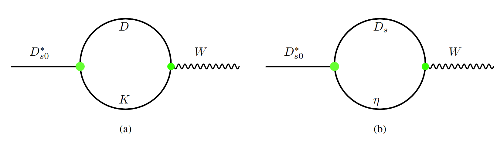
Figure 2: Feynman diagrams for the $W$ boson transiting to $D_{s0}^{*}(2317)$ in the $DK$ and $D_{s}\eta$ molecular picture.

The decay constants $f_{D_{s0}^{*}}$ and $f_{D_{s1}}$ are defined in Eq.(7). To obtain the values of $f_{D_{s0}^{*}}$ and $f_{D_{s1}}$, one usually constructs the amplitudes for the $D_{s0}^{*}$ and $D_{s1}$ created from the vacuum and then extracts the coefficients of $p^{\mu}_{D_{s0}^{*+}}$ and $m_{D_{s1}^{+}}\epsilon_{\mu}^{*}$ Colangelo et al. (1991); Cheng et al. (2004); Thomas (2006); Colangelo et al. (2005). Following the same principle, we calculate the $f_{D_{s0}^{*}}$ and $f_{D_{s1}}$ decay constants in the molecular picture. Assuming that $D_{s0}^{*}$ is dynamically generated by the $DK$ and $D_{s}\eta$ coupled-channel interactions, the current matrix element $\left\langle D_{s0}^{*+}|(s\bar{c})|0\right\rangle$ is illustrated in Fig. 2. Considering HQSS, we replace the above $D$ and $D_{s}$ mesons with the $D^{*}$ and $D_{s}^{*}$ mesons, dynamically generating the $D_{s1}$. In the following, we introduce the effective Lagrangian approach to calculate the decay constants of molecules.

The effective Lagrangians for the $D^{(\ast)}(D_{s}^{(\ast)})$ mesons transiting to the $K(\eta)$ mesons and $W$ boson are given by

$$\mathcal{L}_{VDK} = f_{1}^{DK}(0)V^{\mu}(D\partial_{\mu}K-\partial_{\mu}DK),~{}~{}~{}\mathcal{L}_{VD_{s}\eta}=f_{1}^{D_{s}\eta}(0)V^{\mu}(D_{s}\partial_{\mu}\eta-\partial_{\mu}D_{s}\eta)$$ (12)

$$\mathcal{L}_{AD^{*}K} = (m_{D}+m_{K^{*}})A_{1}^{DK^{*}}(0)A^{\mu}D^{*}_{\mu}K,~{}~{}~{}\mathcal{L}_{AD_{s}^{*}\eta}=(m_{D_{s}}+m_{\phi})A_{1}^{D_{s}\phi}(0)A^{\mu}D^{*}_{s\mu}\eta$$

where $f_{1}^{DK}(0)[f_{1}^{D_{s}\eta}(0)]$ and $A_{1}^{DK^{*}}(0)[A_{1}^{D_{s}\phi}]$ are the form factors at $q^{2}=0$. Such parameters can be determined by fitting the corresponding semileptonic branching fractions. In this work, we take the following values: $f_{0}^{DK}=0.74$ Cheng and Chiang (2010); Cheng et al. (2016); Zhang et al. (2018), $A_{1}^{DK^{*}}=0.78$, $A_{1}^{D_{s}\phi}=0.77$ Chang et al. (2019), $F_{+}^{DK}=0.77$, $F_{+}^{D_{s}\eta}=0.49$, $A_{0}^{DK^{*}}=2.08$, $A_{0}^{D_{s}\phi}=2.13$  Ivanov et al. (2019)

The effective Lagrangians describing the couplings of the hadronic molecules to their constituents are written as

$$\mathcal{L}_{D_{s0}^{*}DK} = g_{D_{s0}^{*}DK}D_{s0}^{*}DK,~{}~{}~{}~{}\mathcal{L}_{D_{s0}^{*}D_{s}\eta}=g_{D_{s0}^{*}D_{s}\eta}D_{s0}^{*}D_{s}\eta$$ (13)

$$\mathcal{L}_{D_{s1}D^{*}K} = g_{D_{s1}D^{*}K}D_{s1}^{\mu}D^{*}_{\mu}K,~{}~{}\mathcal{L}_{D_{s1}D_{s}^{*}\eta}=g_{D_{s1}D_{s}^{*}\eta}D_{s1}^{\mu}D_{s\mu}^{*}K,$$

where $g_{D_{s0}^{*}DK}$, $g_{D_{s0}^{*}D_{s}\eta}$, $g_{D_{s1}D^{*}K}$, and $g_{D_{s1}D_{s}^{*}\eta}$ are the coupling constants between $D_{s0}^{*}(D_{s1})$ and their constituents. In this work, we employ the contact-range EFT to dynamically generate the $D_{s0}^{*}$ and $D_{s1}$ and further determine the couplings between the molecular states and their constituents from the residues of the corresponding poles, which are widely applied to study hadronic molecules Xiao et al. (2019); Du et al. (2020); Pan et al. (2023).

With the above preparations, we can write the amplitude of Fig. 2 as

$$\mathcal{A}_{a} = g_{D_{s0}^{*}DK}f_{1}^{DK}(0)\int\frac{d^{4}q}{(2\pi)^{4}}\frac{1}{k_{1}^{2}-m_{1}^{2}}\frac{1}{k_{2}^{2}-m_{2}^{2}}(k_{1}^{\mu}-k_{2}^{\mu})\varepsilon_{\mu}(V),$$ (14)

$$\mathcal{A}_{b} = g_{D_{s0}^{*}D_{s}\eta}f_{1}^{D_{s}\eta}(0)\int\frac{d^{4}q}{(2\pi)^{4}}\frac{1}{k_{1}^{2}-m_{1}^{2}}\frac{1}{k_{2}^{2}-m_{2}^{2}}(k_{1}^{\mu}-k_{2}^{\mu})\varepsilon_{\mu}(V),$$

where the subscripts 1 and 2 denote the $D$ and $K$ mesons in amplitude $\mathcal{A}_{a}$, and the $D_{s}$ and $\eta$ mesons in amplitude $\mathcal{A}_{b}$. Similarly, we obtain the amplitudes describing the $D_{s1}$ created from the vacuum as

$$\mathcal{A}_{a} = g_{D_{s1}D^{*}K}(m_{D}+m_{K^{*}})A_{1}^{DK^{*}}(0)\int\frac{d^{4}q}{(2\pi)^{4}}\varepsilon_{\mu}(k_{0})\frac{-g^{\mu\nu}+\frac{k_{1}^{\mu}k_{1}^{\nu}}{m_{1}^{2}}}{k_{1}^{2}-m_{1}^{2}}\frac{1}{k_{2}^{2}-m_{2}^{2}}\varepsilon_{\nu}(A),$$ (15)

$$\mathcal{A}_{b} = g_{D_{s1}D_{s}^{*}\eta}(m_{D_{s}}+m_{\phi})A_{1}^{D_{s}\phi}(0)\int\frac{d^{4}q}{(2\pi)^{4}}\varepsilon_{\mu}(k_{0})\frac{-g^{\mu\nu}+\frac{k_{1}^{\mu}k_{1}^{\nu}}{m_{1}^{2}}}{k_{1}^{2}-m_{1}^{2}}\frac{1}{k_{2}^{2}-m_{2}^{2}}\varepsilon_{\nu}(A).$$

Once the amplitudes of Fig. 2 are obtained, the decay constants $f_{D_{s0}^{*}}$ and $f_{D_{s1}}$ can be easily extracted considering their definitions. In the following, we show how to calculate the relevant loop functions in the dimensional regularisation scheme.

With the Feynman parameter approach, we obtain the following integrals

$$\int\frac{d^{4}k_{1}}{(2\pi)^{4}}\frac{1}{(k_{1}^{2}-m_{1}^{2})} = \frac{m_{1}^{2}}{16\pi^{2}}(ln\frac{m_{1}^{2}}{\mu^{2}}-1),$$ (16)

$$\int\frac{d^{4}k_{1}}{(2\pi)^{4}}\frac{1}{(k_{1}^{2}-m_{1}^{2})[(p-k_{1})^{2}-m_{2}^{2}]} = \frac{1}{16\pi^{2}}\int_{0}^{1}dxln\frac{\Delta^{2}}{\mu^{2}},$$

$$\int\frac{d^{4}k}{(2\pi)^{4}}\frac{k^{2}}{(k_{1}^{2}-m_{1}^{2})[(p-k_{1})^{2}-m_{2}^{2}]} = \frac{1}{16\pi^{2}}\int_{0}^{1}dx[\Delta^{2}(2(ln\frac{\Delta^{2}}{\mu^{2}}-1)+1)+p^{2}x^{2}ln\frac{\Delta^{2}}{\mu^{2}}],$$

$$\int\frac{d^{4}k}{(2\pi)^{4}}\frac{k_{1}^{\mu}k_{1}^{\nu}}{(k_{1}^{2}-m_{1}^{2})[(p-k_{1})^{2}-m_{2}^{2}]} = \frac{1}{16\pi^{2}}\int_{0}^{1}dx[g^{\mu\nu}\frac{\Delta^{2}}{2}\,(ln\frac{\Delta^{2}}{\mu^{2}}-1)+p^{\mu}p^{\nu}x^{2}\,ln\frac{\Delta^{2}}{\mu^{2}}],$$

where $\Delta^{2}=p^{2}x^{2}-m_{1}^{2}(x-1)-x(p^{2}-m_{2}^{2})$, $p=k_{1}+k_{2}$, and the renormalization scale $\mu$ depends on the specific physical process under consideration. To extract the decay constants of $D_{s0}^{*}(2317)$ and $D_{s1}(2460)$, the loop functions of Eq. (14) and Eq. (15) are converted into the following form

$$\int\frac{d^{4}k_{1}}{(2\pi)^{4}}\frac{k_{1}^{\mu}-k_{2}^{\mu}}{(k_{1}^{2}-m_{1}^{2})[(p-k_{1})^{2}-m_{2}^{2}]}=\frac{p^{\mu}}{16\pi^{2}}\int_{0}^{1}dx(2x-1)ln\frac{\Delta^{2}}{\mu^{2}},$$ (17)

$$\int\frac{d^{4}k_{1}}{(2\pi)^{4}}\frac{-g^{\mu\nu}+\frac{k_{1}^{\mu}k_{1}^{\nu}}{m_{1}^{2}}}{(k_{1}^{2}-m_{1}^{2})[(p-k_{1})^{2}-m_{2}^{2}]}=-\frac{1}{16\pi^{2}}\int_{0}^{1}dx\{g^{\mu\nu}\left[ln\frac{\Delta^{2}}{\mu^{2}}-\frac{1}{2m_{1}^{2}}\Delta^{2}(ln\frac{\Delta^{2}}{\mu^{2}}-1)\right]$$

$$~{}~{}~{}~{}~{}~{}~{}~{}~{}~{}~{}~{}~{}~{}~{}~{}~{}~{}~{}~{}~{}~{}~{}~{}~{}~{}~{}~{}~{}~{}~{}~{}~{}~{}~{}~{}~{}~{}~{}~{}~{}~{}~{}~{}~{}~{}~{}~{}~{}~{}~{}~{}~{}~{}~{}~{}~{}~{}~{}~{}~{}~{}~{}~{}~{}-\frac{1}{m_{1}^{2}}p^{\mu}p^{\nu}x^{2}ln\frac{\Delta^{2}}{\mu^{2}}\}.$$

Finally, we obtain the analytic form of the decay constants of $D_{s0}^{*}(2317)$ and $D_{s1}(2460)$

$$f_{D_{s0}^{*}}^{m_{1}m_{2}} = g_{D_{s0}^{*}m_{1}m_{2}}f_{1}^{m_{1}m_{2}}(0)\frac{1}{16\pi^{2}}\int_{0}^{1}dx(2x-1)ln\frac{\Delta^{2}}{\mu^{2}},$$ (18)

$$f_{D_{s1}}^{m_{1}m_{2}} = \frac{g_{D_{s1}m_{1}m_{2}}(m_{1}+m_{2})A_{1}^{m_{1}m_{2}}(0)}{m_{D_{s1}}}\frac{1}{16\pi^{2}}\int_{0}^{1}dx~{}\left[\frac{1}{2m_{1}^{2}}\Delta^{2}(ln\frac{\Delta^{2}}{\mu^{2}}-1)-ln\frac{\Delta^{2}}{\mu^{2}}\right],$$ (19)

where $m_{1}$ and $m_{2}$ refer to $D(D_{s})$ and $K(\eta)$ for $D_{s0}^{*}(2317)$ and $D^{*}(D_{s}^{*})$ and $K(\eta)$ for $D_{s1}(2460)$. The decay constants of $D_{s0}^{*}(2317)$ and $D_{s1}(2460)$ are calculated as the sum of $f_{D_{s0}^{*}}^{DK}$ and $f_{D_{s0}^{*}}^{D_{s}\eta}$ and the sum of $f_{D_{s1}}^{D^{*}K}$ and $f_{D_{s1}}^{D_{s}^{*}\eta}$.

II.3 Contact-range effective field theory approach

In the following, we briefly introduce the contact-range effective field theory (EFT) approach. The scattering amplitude $T$ is responsible for the dynamical generations of molecules, which is obtained by solving the following Lippmann-Schwinger equation

$$T(\sqrt{s})=(1-VG(\sqrt{s}))^{-1}V,$$ (20)

where $V$ is the coupled-channel potential determined by the contact-range EFT approach, and $G(\sqrt{s})$ is the loop function of the two-body propagator.

The coupled-channel potential $V$ in matrix form reads

$$V_{DK-D_{s}\eta}^{J^{P}=0^{+}}=\begin{pmatrix}-2C_{a}&\sqrt{3}C_{a}\\ \sqrt{3}C_{a}&0\end{pmatrix},\quad V_{D^{*}K-D_{s}^{*}\eta}^{J^{P}=1^{+}}=\varepsilon(k_{1})\cdot\varepsilon(k_{1}^{\prime})\begin{pmatrix}-2C_{a}&\sqrt{3}C_{a}\\ \sqrt{3}C_{a}&0\end{pmatrix},$$ (21)

where the coefficient $C_{a}$ needs to be determined by fitting the $D_{s0}^{*}$ and $D_{s1}$ masses. The loop functions of $D_{s0}^{*}$ and $D_{s1}$ are

$$G(\sqrt{s})^{D_{s0}^{*}} = \frac{1}{16\pi^{2}}\int_{0}^{1}dxln\frac{\Delta^{2}}{\mu^{2}},$$ (22)

$$G(\sqrt{s})^{D_{s1}} = \frac{1}{16\pi^{2}}\int_{0}^{1}dx~{}\left[ln\frac{\Delta^{2}}{\mu^{2}}-\frac{1}{2m_{1}^{2}}\Delta^{2}(ln\frac{\Delta^{2}}{\mu^{2}}-1)\right]$$

with $\Delta^{2}=sx^{2}-m_{1}^{2}(x-1)-x(s-m_{2}^{2})$. We note that the loop function of $D_{s1}$ contains an additional term, which is induced by the $\frac{k_{1}^{\mu}k_{1}^{\nu}}{m_{1}^{2}}$ term in the loop integral. One can see that the loop integrals depend on the renormalization scale $\mu$.

With the potentials obtained above, we can search for poles generated by the coupled-channel interactions and determine the couplings between the molecular states and their constituents from the residues of the corresponding poles,

$$g_{i}g_{j}=\lim_{\sqrt{s}\to\sqrt{s_{0}}}\left(\sqrt{s}-\sqrt{s_{0}}\right)T_{ij}(\sqrt{s}),$$ (23)

where $g_{i}$ denotes the coupling of channel $i$ to the dynamically generated state and $\sqrt{s_{0}}$ is the pole position.

III Results and Discussions

Table 1: Masses and quantum numbers of relevant hadrons needed in this work Workman et al. (2022).

Hadron	$I(J^{P})$	M (MeV)	Hadron	$I(J^{P})$	M (MeV)	Hadron	$I(J^{P})$	M (MeV)
$K^{\pm}$	$1/2(0^{-})$	$493.677$	$K^{0}$	$1/2(0^{-})$	$497.611$	$\Lambda_{b}$	$0(1/2^{+})$	$5619.60$
$\bar{D}^{0}$	$1/2(0^{-})$	$1864.84$	$D^{-}$	$1/2(0^{-})$	$1869.66$	$\Lambda_{c}^{+}$	$0(1/2^{+})$	$2286.46$
$\bar{D}^{\ast 0}$	$1/2(1^{-})$	$2006.85$	$D^{\ast-}$	$1/2(1^{-})$	$2010.26$	$B^{+}$	$1/2(0^{-})$	$5279.34$
$J/\psi$	$0(1^{-})$	$3096.90$	$\eta_{c}$	$0(0^{-})$	$2983.90$	$B^{0}$	$1/2(0^{-})$	$5279.65$
$D_{s}^{\pm}$	$0(0^{-})$	$1968.35$	$D_{s}^{\ast\pm}$	$0(1^{-})$	$2112.2$	$B_{s}^{0}$	$0(0^{-})$	$5366.91$

In Table 1, we tabulate the masses and quantum numbers of relevant particles. One can see that there exists an unknown parameter $\mu$ (renormalization scale) in both Eq. (17) and Eq. (22), for which a consistent value is adopted in this work. First, we employ the contact-range EFT approach to dynamically generate the poles corresponding to $D_{s0}^{*}(2317)$ and $D_{s1}(2460)$ by varying $\mu$ and then obtain the $D_{s0}^{*}(2317)$ and $D_{s1}(2460)$ couplings to their constituents as well as their decay constants. With the so-obtained decay constants $f_{D_{s0^{*}}(2317)}$ and $f_{D_{s1}(2460)}$ we further study the productions of $D_{s0}^{*}(2317)$ and $D_{s1}(2460)$ in the $B_{(s)}$ and $\Lambda_{b}(\Xi_{b})$ decays, where the naive factorization approach works well as mentioned above. In this work, assuming that the decay mechanisms of $H_{b}\to H_{c}D_{s}^{(\ast)}$($H_{b}$ and $H_{c}$ denote bottom and charm hadrons of interest) and $H_{b}\to H_{c}D_{s0}^{*}(D_{s1})$ are the same, we parameterize the unknown non-factorization contributions with the effective Wilson coefficients. In other words, we determine $a_{1}$ by reproducing the experimental branching fractions of $H_{b}\to H_{c}D_{s}^{(\ast)}$ decays, and then calculate the branching fractions of the corresponding decays $H_{b}\to H_{c}D_{s0}^{*}(D_{s1})$ using the so-obtained $a_{1}$.

Table 2: $D_{s0}^{*}(2317)$ and $D_{s1}(2460)$ couplings to their constituents (in units of MeV).

Couplings	$\mu=1000$	$\mu=1500$	$\mu=2000$	Fu et al. Fu et al. (2022)
$g_{D_{s0}^{*}DK}$	11.75	11.92	11.95	9.4
$g_{D_{s0}^{*}D_{s}\eta}$	8.13	7.47	7.32	7.4
$g_{D_{s1}D^{*}K}$	12.06	12.16	12.15	10.1
$g_{D_{s1}D_{s}^{*}\eta}$	8.78	7.76	7.53	7.9

In Refs. Gamermann et al. (2007); Molina et al. (2010); Chen et al. (2023), the loop function is regularised in the dimensional regularization scheme, which shows that $\mu$ is around $1.5$ GeV in the charm sector. To quantify the uncertainty of the renormalization scale, we vary $\mu$ from $1$ GeV to $2$ GeV in this work. For $\mu$ of $1.0$ GeV, $1.5$ GeV, and $2.0$ GeV, the values of $C_{a}$ for $DK-D_{s}\eta$ ($D^{*}K-D_{s}^{*}\eta$) contact-range potentials are determined as $74.78$, $34.53$, and $25.04$ ($98.60$, $42.45$, and $30.34$). With the so-obtained scattering amplitude $T$, we obtain the $D_{s0}^{*}(2317)$ and $D_{s1}(2460)$ couplings to their constituents shown in Table 2, a bit different from the estimations of Ref. Fu et al. (2022). Finally, the decays constants of $D_{s0}^{*}(2317)$ and $D_{s1}(2460)$ are determined as shown in Table 3. One can see that $f_{D_{s0}^{*}(2317)}$ is almost independent of the renormalization scale, as can also seen from Eq. (18). The slight variation of $f_{D_{s0}^{*}(2317)}$ stems from the weak dependence of the couplings $g_{D_{s0}^{*}DK}$ and $g_{D_{s0}^{*}D_{s}\eta}$ on the renormalization scale $\mu$. However, the decay constant $f_{D_{s1}(2460)}$ is dependent on $\mu$ as shown in Table 3. In the following calculations, we adopt the values of $f_{D_{s0^{*}}(2317)}$ and $f_{D_{s1}(2460)}$ at $\mu=1.5$ GeV, e.g., $f_{D_{s0}^{*}}=58.74$ GeV and $f_{D_{s1}}=133.76$ GeV, which are consistent with the results of Ref. Faessler et al. (2007c), but smaller than the results of lattice QCD Bali et al. (2017).

Table 3: Decay constants of $D_{s0}^{*}(2317)$ and $D_{s1}(2460)$ as hadronic molecules (in units of MeV).

Decay Constants	$\mu=1000$	$\mu=1500$	$\mu=2000$	Faessler et al. Faessler et al. (2007c)
$f_{D_{s0}^{*}(2317)}$	59.36	58.74	58.59	67.1
$f_{D_{s1}(2460)}$	56.10	133.76	187.48	144.5

Table 4: Values of $F(0)^{B\to D^{(*)}}$, $a^{B\to D^{(*)}}$, $b^{B\to D^{(*)}}$ in the $B\rightarrow D^{(*)}$ transition form factors and $F(0)^{B_{s}\to D_{s}^{(*)}}$, $a^{B_{s}\to D_{s}^{(*)}}$, $b^{B_{s}\to D_{s}^{(*)}}$ in the ${B_{s}\to D_{s}^{(*)}}$ transition form factors Verma (2012).

	$F_{0}$	$F_{1}$	$V$	$A_{0}$	$A_{1}$	$A_{2}$		$F_{0}$	$F_{1}$	$V$	$A_{0}$	$A_{1}$	$A_{2}$
$F(0)^{B\to D^{(*)}}$	0.67	0.67	0.77	0.68	0.65	0.61	$F(0)^{B_{s}\to D_{s}^{(*)}}$	0.67	0.67	0.75	0.66	0.62	0.57
$a^{B\to D^{(*)}}$	0.63	1.22	1.25	1.21	0.60	1.12	$a^{B_{s}\to D_{s}^{(*)}}$	0.69	1.28	1.37	1.33	0.76	1.25
$b^{B\to D^{(*)}}$	-0.01	0.36	0.38	0.36	0.00	0.31	$b^{B_{s}\to D_{s}^{(*)}}$	0.07	0.52	0.67	0.63	0.13	0.56

Up to now, $D_{s0}^{*}(2317)$ and $D_{s1}(2460)$ have only been observed in $B$ decays. Therefore, we first focus on the decays of $B\to\bar{D}^{(\ast)}D_{s}^{(\ast)}$ and $B\to\bar{D}^{(\ast)}D_{s0}^{*}(D_{s1})$. In Table 4, we present the parameters of the form factors in the $B\to D$ and $B\to D^{*}$ transitions, which are taken from Ref. Verma (2012). By reproducing the experimental branching fractions of the decays $B\to\bar{D}^{(\ast)}D_{s}^{(\ast)}$, we determine the effective Wilson coefficient $a_{1}$. Using $a_{1}$ and $f_{D_{s0}^{*}}(f_{D_{s}})$ obtained above, we calculate the branching fractions of the decays $B\to\bar{D}^{(\ast)}D_{s0}(D_{s1})$ , which are shown in Table 5. Our results are a bit smaller than those of Ref. Faessler et al. (2007c) because of the smaller values for the decay constants and the effective Wilson coefficient. Interestingly, our results are consistent with our previous calculations using the triangle mechanism for the decay $B^{+}\to\bar{D}^{\ast 0}D_{s0}^{*+}$ Liu et al. (2022) , which indicates that the triangle diagram and tree diagram accounting for the decays $B\to\bar{D}^{(\ast)}D_{s0}(D_{s1})$ are equivalent. In principle, one can replace the triangle diagram with one vertex, resulting in an effective description for the weak decay $B^{+}\to\bar{D}^{0}D_{s0}^{*+}(2317)$ at tree level as shown in Fig. 3, which indicates that it is reasonable to extract the decay constants of hadronic molecules using the triangle mechanism. In Ref. Wu et al. (2023), with this approach, we extract the decay constants of $X(3872)$ as a $\bar{D}D^{*}$ molecule. Here, we note that the relative phase among various amplitudes may lead to uncertainties in extracting the decay constants. As a result, it is better to select relevant amplitudes with no or small relative phases.

Table 5: Branching fractions of ($10^{-3}$) of $B\to\bar{D}^{(\ast)}D_{s0}(D_{s1})$.

Decay modes	Exp Workman et al. (2022)	$a_{1}$	Decay modes	$\mathrm{Ours}$	Triangle Liu et al. (2022)	Exp Workman et al. (2022)
$B^{+}\to\bar{D}^{0}D_{s}^{+}$	$9.0\pm 0.9$	0.80	$B^{+}\to\bar{D}^{0}D_{s0}^{*+}(2317)$	$0.48$	$0.68$	$0.80^{+0.16}_{-0.13}$
$B^{+}\to\bar{D}^{\ast 0}D_{s}^{+}$	$8.2\pm 1.7$	0.93	$B^{+}\to\bar{D}^{\ast 0}D_{s0}(2317)$	$0.39$	$1.21$	$0.90^{+0.70}_{-0.70}$
$B^{+}\to\bar{D}^{0}D_{s}^{\ast+}$	$7.6\pm 1.6$	0.81	$B^{+}\to\bar{D}^{0}D_{s1}(2460)$	$1.39$	$1.26$	$3.1^{+1.0}_{-0.9}$
$B^{+}\to\bar{D}^{\ast 0}D_{s}^{\ast+}$	$17.1\pm 2.4$	0.83	$B^{+}\to\bar{D}^{\ast 0}D_{s1}(2460)$	$4.36$	$3.07$	$12.0\pm 3.0$

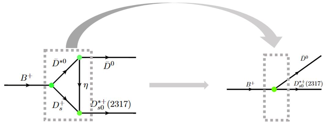
Figure 3: Equivalence of the triangle diagram and the tree diagram depict the decay of $B^{+}\to\bar{D}^{0}D_{s0}^{*+}(2317)$.

Along this line, we investigate the decays of $B_{s}\to\bar{D}_{s}^{(*)}D_{s}^{(*)}$ and $B_{s}\to\bar{D}_{s0}^{*}(\bar{D}_{s1})D_{s}^{(*)}$, which are related to the decays of $B\to\bar{D}^{(\ast)}D_{s}^{(\ast)}$ and $B\to\bar{D}^{(\ast)}D_{s0}^{*}(D_{s1})$ via SU(3)-flavor symmetry as shown in Fig. 1. The amplitudes for the decays of $B_{s}\to\bar{D}_{s}^{(*)}D_{s}^{(*)}$ and $B_{s}\to\bar{D}_{s0}^{*}(\bar{D}_{s1})D_{s}^{(*)}$ are the same as those of their SU(3) symmetric partners. The unknown parameters in the form factors of the $B_{s}\to D_{s}^{(*)}$ transitions are taken from Ref. Verma (2012), tabulated in Table 4. Following the same strategy, we calculate the branching fractions of the decays $B_{s}\to\bar{D}_{s}^{(\ast)}D_{s0}^{*}$ and $B_{s}\to\bar{D}_{s}^{(\ast)}D_{s1}$. The results are shown in Table 6. One can see that the branching fractions of $D_{s0}^{*}(2317)$ and $D_{s1}(2460)$ in the $B_{s}$ decays are similar to those in the $B$ decays, following the SU(3)-flavor symmetry. Such large production rates means that the $D_{s0}^{*}(2317)$ and $D_{s1}(2460)$ are likely to be detected in future experiments.

Table 6: Branching ratios ($10^{-3}$) of $B\to\bar{D}_{s}^{(\ast)}D_{s0}(D_{s1})$.

decay modes	Exp Workman et al. (2022)	$a_{1}$	decay modes	$\mathrm{Ours}$
$B_{s}^{0}\to D_{s}^{+}D_{s}^{-}$	$4.4\pm 0.5$	0.87	$B_{s}^{0}\to D_{s}D_{s0}^{\ast}(2317)$	$0.47$
$B_{s}^{0}\to D_{s}^{\ast+}D_{s}^{-}+D_{s}^{+}D_{s}^{\ast-}$	$13.9\pm 1.7$	0.83	$B_{s}^{0}\to D_{s}^{*}D_{s0}(2317)$	$0.27$
$B_{s}^{0}\to D_{s}^{\ast+}D_{s}^{-}+D_{s}^{+}D_{s}^{\ast-}$	$13.9\pm 1.7$	0.77	$B_{s}^{0}\to{D}_{s}D_{s1}(2460)$	$1.18$
$B_{s}^{0}\to D_{s}^{\ast+}D_{s}^{\ast-}$	$14.4\pm 2.1$	0.84	$B_{s}^{0}\to D_{s}^{\ast}D_{s1}(2460)$	$4.11$

In addition to the productions of $D_{s0}^{*}(2317)$ and $D_{s1}(2460)$ in the $B_{(s)}$ decays, it is interesting to investigate their productions in the $\Lambda_{b}$($\Xi_{b}$) decays. As indicated in Fig. 1, the decays of $\Lambda_{b}\to D_{s}^{(\ast)}\Lambda_{c}$ and $\Lambda_{b}\to D_{s0}^{*}(D_{s1})\Lambda_{c}$ share the same mechanism as those of $B\to D_{s}^{(\ast)}\bar{D}^{(*)}$ and $B\to D_{s0}^{*}(D_{s1})\bar{D}^{(*)}$ at quark level, which proceeds via the decays $b\to c\bar{c}s$. In terms of SU(3)-flavor symmetry, we also investigate the decays of $\Xi_{b}\to D_{s}^{(\ast)}\Xi_{c}$ and $\Xi_{b}\to D_{s0}^{*}(D_{s1})\Xi_{c}$. With the naive factorization approach, the amplitudes for these decays are given by the effective Lagrangian shown in Eq. (9), where the parameters in the form factors of the $\Lambda_{b}\to\Lambda_{c}$ and $\Xi_{b}\to\Xi_{c}$ transitions are obtained in the quark model Gutsche et al. (2015); Faustov and Galkin (2018); Lu et al. (2021), tabulated in Table 7. The decay constants of the charmed-strange mesons $D_{s}^{(*)}$ and $D_{s0}^{*}(D_{s1})$ are calculated in the same way as explained above.

Table 7: Values of $F(0)$, $a$, $b$ in the $\Lambda_{b}\rightarrow\Lambda_{c}$ and $\Xi_{b}\rightarrow\Xi_{c}$ transition form factors Gutsche et al. (2015); Faustov and Galkin (2018).

	$F_{1}^{V}$	$F_{2}^{V}$	$F_{3}^{V}$	$F_{1}^{A}$	$F_{2}^{A}$	$F_{3}^{A}$
$F(0)^{\Lambda_{b}\to\Lambda_{c}}$	0.549	0.110	$-0.023$	0.542	0.018	$-0.123$
$a^{\Lambda_{b}\to\Lambda_{c}}$	1.459	1.680	1.181	1.443	0.921	1.714
$b^{\Lambda_{b}\to\Lambda_{c}}$	0.571	0.794	0.276	0.559	0.255	0.828
$F(0)^{\Xi_{b}\to\Xi_{c}}$	0.467	0.145	$0.086$	0.447	$-0.035$	$-0.278$
$a^{\Xi_{b}\to\Xi_{c}}$	1.702	2.530	1.742	1.759	2.675	2.270
$b^{\Xi_{b}\to\Xi_{c}}$	0.531	1.581	0.758	0.356	1.789	1.072

Table 8: Branching fractions ($10^{-3}$) of $\Lambda_{b}\to\Lambda_{c}D_{s0}^{*}(D_{s1})$ and $\Xi_{b}\to\Xi_{c}D_{s0}^{*}(D_{s1})$.

decay modes	Exp Workman et al. (2022); Aaij et al. (2023)	$a_{1}$	decay modes	Ours
$\Lambda_{b}\to\Lambda_{c}D_{s}^{-}$	$11\pm 1.0$	$0.88$	$\Lambda_{b}\to\Lambda_{c}D_{s0}^{*}(2317)$	$0.70$
$\Lambda_{b}\to\Lambda_{c}D_{s}^{\ast-}$	$18.568\pm 1.102$	$0.76$	$\Lambda_{b}\to\Lambda_{c}D_{s1}(2460)$	$4.34$
decay modes	Ours	$a_{1}$	decay modes	Ours
$\Xi_{b}\to\Xi_{c}D_{s}^{-}$	$8.52$	$0.88$	$\Xi_{b}\to\Xi_{c}D_{s0}^{*}(2317)$	$0.58$
$\Xi_{b}\to\Xi_{c}D_{s}^{\ast-}$	$16.30$	$0.76$	$\Xi_{b}\to\Xi_{c}D_{s1}(2460)$	$4.29$

One should note that only the branching fraction of the decay $\Lambda_{b}\to D_{s}\Lambda_{c}$ is available in the RPP. Very recently the ratio of $\mathcal{B}(\Lambda_{b}\to D_{s}^{*}\Lambda_{c})/\mathcal{B}(\Lambda_{b}\to D_{s}\Lambda_{c})=1.688\pm 0.022^{+0.061}_{-0.055}$ is reported by the LHCb Collaboration Aaij et al. (2023), and one can obtain the branching fraction of the decay $\Lambda_{b}\to D_{s}^{*}\Lambda_{c}$. With the branching fractions of $\mathcal{B}(\Lambda_{b}\to D_{s}\Lambda_{c})$ and $\mathcal{B}(\Lambda_{b}\to D_{s}^{*}\Lambda_{c})$ as inputs, we determine $a_{1}$, and then predict the branching fractions of the decays of $\Lambda_{b}\to D_{s0}^{*}\Lambda_{c}$ and $\Lambda_{b}\to D_{s1}\Lambda_{c}$, which are shown in Table 8. We can see that the production rates of $D_{s0}^{*}(2317)$ and $D_{s1}(2460)$ in the $\Lambda_{b}$ decay are of the order of $10^{-3}$, which are large enough to be detected in future experiments. Since the effective Wilson coefficients in the $B$ decays and $B_{s}$ decays are similar, as shown in Table 5 and Table 6, we can take the same values for $a_{1}$ in the $\Lambda_{b}$ decays and the $\Xi_{b}$ decays. Similarly, we predict the branching fractions of the decays $\Xi_{b}\to D_{s}^{(\ast)}\Xi_{c}$ and $\Xi_{b}\to D_{s0}^{*}(D_{s1})\Xi_{c}$ in Table 8. The production rates of ground-state mesons $D_{s}^{(*)}$ and excited mesons $D_{s0}^{*}(D_{s1})$ in the $\Xi_{b}$ decays are of the order of $10^{-2}$ and $10^{-3}$,, which are likely to be detected in future experiments. In Ref. Datta et al. (2004), the authors estimated the ratios $\mathcal{B}(\Lambda_{b}\to\Lambda_{c}M)/\mathcal{B}(B\to DM)$, where $M$ represents the ground-state $D_{s}^{(*)}$ and excited $D_{s0}^{*}(D_{s1})$ mesons. In Table 9, we show the ratios $R_{u}^{M}=\mathcal{B}(\Lambda_{b}\to\Lambda_{c}M)/\mathcal{B}(B\to DM)$ and $R_{s}^{M}=\mathcal{B}(\Xi_{b}\to\Xi_{c}M)/\mathcal{B}(B_{s}\to D_{s}M)$ obtained in this work, which are consistent with Ref. Datta et al. (2004). We can see that the production rates of ground-state mesons $D_{s}^{(*)}$ and excited mesons $D_{s0}^{*}(D_{s1})$ in the $\Lambda_{b}(\Xi_{b})$ decays are larger than those in the $B_{(s)}$ decays because the $\Lambda_{b}\to\Lambda_{c}$($\Xi_{b}\to\Xi_{c}$) form factors are larger than the corresponding $B_{(s)}\to D_{(s)}$ form factor as shown in Ref. Datta et al. (2004).

Table 9: Ratios of $R_{u}^{M}=\mathcal{B}(\Lambda_{b}\to\Lambda_{c}M)/\mathcal{B}(B\to DM)$ and $R_{s}^{M}=\mathcal{B}(\Xi_{b}\to\Xi_{c}M)/\mathcal{B}(B_{s}\to D_{s}M)$.

$R_{u}^{M}$	Ours	Ref. Datta et al. (2004)	$R_{s}^{M}$	Ours
$R_{u}^{D_{s}}$	$1.22$	$1.75$	$R_{s}^{D_{s}}$	1.94
$R_{u}^{D_{s}^{\ast}}$	$2.44$	$3.47$	$R_{s}^{D_{s}^{\ast}}$	$2.35$
$R_{u}^{D_{s0}^{\ast}}$	$1.46$	$1.58$	$R_{s}^{D_{s0}^{\ast}}$	$1.23$
$R_{u}^{D_{s1}}$	$3.12$	$4.76$	$R_{s}^{D_{s1}}$	$3.64$

IV Summary and outlook

In this work, we utilized the effective Lagrangian approach to compute the decay constants of $D_{s0}^{\ast}(2317)$ and $D_{s1}(2460)$ as hadronic molecules dynamically generated by the $DK-D_{s}\eta$ and $D^{*}K-D_{s}^{*}\eta$ contact-range potentials, and then with the naive factorization approach systematically investigated the productions of $D_{s0}^{\ast}(2317)$ and $D_{s1}(2460)$ in the $B_{(s)}$ and $\Lambda_{b}(\Xi_{b})$ decays, which proceed via the decay $b\to c\bar{c}s$ at quark level. The decay constants of $D_{s0}^{\ast}(2317)$ and $D_{s1}(2460)$ are estimated to be $58.74$ MeV and $133.76$ MeV. In particular, the decay constant of $D_{s0}^{\ast}(2317)$ is almost independent of the renormalization scale $\mu$ in the loop functions.

As for the branching fractions of the decays $B\to\bar{D}^{(*)}D_{s0}^{\ast}(2317)$ and $B\to\bar{D}^{(*)}D_{s1}(2460)$, our results are smaller than the experimental data, but are consistent with our previous results obtained in the triangle mechanism, which indicates that $D_{s0}^{\ast}(2317)$ and $D_{s1}(2460)$ may contain components other than hadronic molecules, such as a $c\bar{s}$ core. The values of $\mathcal{B}[B_{s}\to{D}_{s}^{(*)}D_{s0}^{\ast}(2317)]$ and $\mathcal{B}[B_{s}\to{D}_{s}^{(*)}D_{s1}(2460)]$ are similar to those of $\mathcal{B}[B\to\bar{D}^{(*)}D_{s0}^{\ast}(2317)]$ and $\mathcal{B}[B\to\bar{D}^{(*)}D_{s1}(2460)]$, which reflects the underlying SU(3)-flavor symmetry. In addition, we predicted the branching fractions of the decays $\Lambda_{b}\to\Lambda_{c}D_{s0}^{\ast}(2317)$ and $\Lambda_{b}\to\Lambda_{c}D_{s1}(2460)$ as well as $\Xi_{b}\to\Xi_{c}D_{s0}^{\ast}(2317)$ and $\Xi_{b}\to\Xi_{c}D_{s1}(2460)$, which are much larger than the corresponding ones in the $B$ and $B_{s}$ decays and indicates that the productions of $D_{s0}^{\ast}(2317)$ and $D_{s1}(2460)$ in the decays of bottom baryons are likely to be detected in future experiments.

Our study shows that, because of the equivalence of the triangle mechanism to the tree diagram established in calculating the branching fractions of the decays $B\to\bar{D}^{(*)}D_{s0}^{\ast}(2317)$ and $B\to\bar{D}^{(*)}D_{s1}(2460)$, one can extract the decay constants of $D_{s0}^{\ast}(2317)$ and $D_{s1}(2460)$ as hadronic molecules via the triangle mechanism. This provides an effective approach to calculating the decay constants of hadronic molecules, which can then be used in studies of these hadronic molecules in other related processes. We hope that our present work can stimulate more studies along this line.

V Acknowledgments

We are grateful to Prof. Fu-Sheng Yu for stimulating discussions. This work is supported in part by the National Natural Science Foundation of China under Grants No.11975041 and No.11961141004. M.Z.L acknowledges support from the National Natural Science Foundation of China under Grant No.12105007. X.Z.L acknowledges support from the National Natural Science Foundation of China under Grant No. 12247159 and China Postdoctoral Science Foundation under Grant No. 2022M723149.

References

- Aubert et al. (2003) B. Aubert et al. (BaBar), Phys. Rev. Lett. 90, 242001 (2003), arXiv:hep-ex/0304021 .
- Besson et al. (2003) D. Besson et al. (CLEO), Phys. Rev. D 68, 032002 (2003), [Erratum: Phys.Rev.D 75, 119908 (2007)], arXiv:hep-ex/0305100 .
- Mikami et al. (2004) Y. Mikami et al. (Belle), Phys. Rev. Lett. 92, 012002 (2004), arXiv:hep-ex/0307052 .
- Ablikim et al. (2018) M. Ablikim et al. (BESIII), Phys. Rev. D 97, 051103 (2018), arXiv:1711.08293 [hep-ex] .
- Krokovny et al. (2003) P. Krokovny et al. (Belle), Phys. Rev. Lett. 91, 262002 (2003), arXiv:hep-ex/0308019 .
- Aubert et al. (2004a) B. Aubert et al. (BaBar), Phys. Rev. Lett. 93, 181801 (2004a), arXiv:hep-ex/0408041 .
- Aubert et al. (2004b) B. Aubert et al. (BaBar), Phys. Rev. D 69, 031101 (2004b), arXiv:hep-ex/0310050 .
- Godfrey and Isgur (1985) S. Godfrey and N. Isgur, Phys. Rev. D 32, 189 (1985).
- Song et al. (2015) Q.-T. Song, D.-Y. Chen, X. Liu, and T. Matsuki, Phys. Rev. D 91, 054031 (2015), arXiv:1501.03575 [hep-ph] .
- Albaladejo et al. (2018) M. Albaladejo, P. Fernandez-Soler, J. Nieves, and P. G. Ortega, Eur. Phys. J. C 78, 722 (2018), arXiv:1805.07104 [hep-ph] .
- Yang et al. (2022) Z. Yang, G.-J. Wang, J.-J. Wu, M. Oka, and S.-L. Zhu, Phys. Rev. Lett. 128, 112001 (2022), arXiv:2107.04860 [hep-ph] .
- Luo et al. (2021) S.-Q. Luo, B. Chen, X. Liu, and T. Matsuki, Phys. Rev. D 103, 074027 (2021), arXiv:2102.00679 [hep-ph] .
- Barnes et al. (2003) T. Barnes, F. E. Close, and H. J. Lipkin, Phys. Rev. D 68, 054006 (2003), arXiv:hep-ph/0305025 .
- Gamermann et al. (2007) D. Gamermann, E. Oset, D. Strottman, and M. J. Vicente Vacas, Phys. Rev. D76, 074016 (2007), arXiv:hep-ph/0612179 [hep-ph] .
- Guo et al. (2006) F.-K. Guo, P.-N. Shen, H.-C. Chiang, R.-G. Ping, and B.-S. Zou, Phys. Lett. B641, 278 (2006), arXiv:hep-ph/0603072 [hep-ph] .
- Xie et al. (2010) Z.-X. Xie, G.-Q. Feng, and X.-H. Guo, Phys. Rev. D 81, 036014 (2010).
- Cleven et al. (2011) M. Cleven, F.-K. Guo, C. Hanhart, and U.-G. Meissner, Eur. Phys. J. A 47, 19 (2011), arXiv:1009.3804 [hep-ph] .
- Guo et al. (2015) Z.-H. Guo, U.-G. Meißner, and D.-L. Yao, Phys. Rev. D 92, 094008 (2015), arXiv:1507.03123 [hep-ph] .
- Wu et al. (2019) T.-W. Wu, M.-Z. Liu, L.-S. Geng, E. Hiyama, and M. P. Valderrama, Phys. Rev. D100, 034029 (2019), arXiv:1906.11995 [hep-ph] .
- Liu et al. (2013) L. Liu, K. Orginos, F.-K. Guo, C. Hanhart, and U.-G. Meissner, Phys. Rev. D87, 014508 (2013), arXiv:1208.4535 [hep-lat] .
- Mohler et al. (2013) D. Mohler, C. B. Lang, L. Leskovec, S. Prelovsek, and R. M. Woloshyn, Phys. Rev. Lett. 111, 222001 (2013), arXiv:1308.3175 [hep-lat] .
- Lang et al. (2014) C. B. Lang, L. Leskovec, D. Mohler, S. Prelovsek, and R. M. Woloshyn, Phys. Rev. D 90, 034510 (2014), arXiv:1403.8103 [hep-lat] .
- Bali et al. (2017) G. S. Bali, S. Collins, A. Cox, and A. Schäfer, Phys. Rev. D 96, 074501 (2017), arXiv:1706.01247 [hep-lat] .
- Alexandrou et al. (2020) C. Alexandrou, J. Berlin, J. Finkenrath, T. Leontiou, and M. Wagner, Phys. Rev. D 101, 034502 (2020), arXiv:1911.08435 [hep-lat] .
- Weinberg (1965) S. Weinberg, Phys. Rev. 137, B672 (1965).
- Martínez Torres et al. (2015) A. Martínez Torres, E. Oset, S. Prelovsek, and A. Ramos, JHEP 05, 153 (2015), arXiv:1412.1706 [hep-lat] .
- Albaladejo et al. (2016) M. Albaladejo, D. Jido, J. Nieves, and E. Oset, Eur. Phys. J. C 76, 300 (2016), arXiv:1604.01193 [hep-ph] .
- Song et al. (2022) J. Song, L. R. Dai, and E. Oset, Eur. Phys. J. A 58, 133 (2022), arXiv:2201.04414 [hep-ph] .
- Workman et al. (2022) R. L. Workman et al. (Particle Data Group), PTEP 2022, 083C01 (2022).
- Fayyazuddin and Riazuddin (2004) Fayyazuddin and Riazuddin, Phys. Rev. D 69, 114008 (2004), arXiv:hep-ph/0309283 .
- Ishida et al. (2004) S. Ishida, M. Ishida, T. Komada, T. Maeda, M. Oda, K. Yamada, and I. Yamauchi, AIP Conf. Proc. 717, 716 (2004), arXiv:hep-ph/0310061 .
- Wei et al. (2006) W. Wei, P.-Z. Huang, and S.-L. Zhu, Phys. Rev. D 73, 034004 (2006), arXiv:hep-ph/0510039 .
- Nielsen (2006) M. Nielsen, Phys. Lett. B 634, 35 (2006), arXiv:hep-ph/0510277 .
- Faessler et al. (2007a) A. Faessler, T. Gutsche, V. E. Lyubovitskij, and Y.-L. Ma, Phys. Rev. D 76, 014005 (2007a), arXiv:0705.0254 [hep-ph] .
- Faessler et al. (2007b) A. Faessler, T. Gutsche, V. E. Lyubovitskij, and Y.-L. Ma, Phys. Rev. D76, 114008 (2007b), arXiv:0709.3946 [hep-ph] .
- Fu et al. (2022) H.-L. Fu, H. W. Grießhammer, F.-K. Guo, C. Hanhart, and U.-G. Meißner, Eur. Phys. J. A 58, 70 (2022), arXiv:2111.09481 [hep-ph] .
- Huang et al. (2020) Y. Huang, M.-Z. Liu, Y.-W. Pan, L.-S. Geng, A. Martínez Torres, and K. P. Khemchandani, Phys. Rev. D101, 014022 (2020), arXiv:1909.09021 [hep-ph] .
- Wu et al. (2022) T.-W. Wu, Y.-W. Pan, M.-Z. Liu, and L.-S. Geng, Sci. Bull. 67, 1735 (2022), arXiv:2208.00882 [hep-ph] .
- Wu and Geng (2023) T.-C. Wu and L.-S. Geng, Phys. Rev. D 108, 014015 (2023), arXiv:2211.01846 [hep-ph] .
- Aubert et al. (2006) B. Aubert et al. (BaBar), Phys. Rev. D 74, 032007 (2006), arXiv:hep-ex/0604030 .
- Faessler et al. (2007c) A. Faessler, T. Gutsche, S. Kovalenko, and V. E. Lyubovitskij, Phys. Rev. D 76, 014003 (2007c), arXiv:0705.0892 [hep-ph] .
- Colangelo et al. (1991) P. Colangelo, G. Nardulli, A. A. Ovchinnikov, and N. Paver, Phys. Lett. B 269, 201 (1991).
- Veseli and Dunietz (1996) S. Veseli and I. Dunietz, Phys. Rev. D 54, 6803 (1996), arXiv:hep-ph/9607293 .
- Cheng et al. (2004) H.-Y. Cheng, C.-K. Chua, and C.-W. Hwang, Phys. Rev. D 69, 074025 (2004), arXiv:hep-ph/0310359 .
- Colangelo et al. (2005) P. Colangelo, F. De Fazio, and A. Ozpineci, Phys. Rev. D 72, 074004 (2005), arXiv:hep-ph/0505195 .
- Cheng and Chua (2006) H.-Y. Cheng and C.-K. Chua, Phys. Rev. D 74, 034020 (2006), arXiv:hep-ph/0605073 .
- Segovia et al. (2012) J. Segovia, C. Albertus, E. Hernandez, F. Fernandez, and D. R. Entem, Phys. Rev. D 86, 014010 (2012), arXiv:1203.4362 [hep-ph] .
- Datta et al. (2004) A. Datta, H. J. Lipkin, and P. J. O’Donnell, Phys. Rev. D 69, 094002 (2004), arXiv:hep-ph/0312160 .
- Liu et al. (2023) Z.-W. Liu, J.-X. Lu, and L.-S. Geng, Phys. Rev. D 107, 074019 (2023), arXiv:2302.01046 [hep-ph] .
- Ikeno et al. (2023) N. Ikeno, G. Toledo, and E. Oset, Phys. Lett. B 847, 138281 (2023), arXiv:2305.16431 [hep-ph] .
- Adamczyk et al. (2015) L. Adamczyk et al. (STAR), Nature 527, 345 (2015), arXiv:1507.07158 [nucl-ex] .
- Collaboration et al. (2020) A. Collaboration et al. (ALICE), Nature 588, 232 (2020), [Erratum: Nature 590, E13 (2021)], arXiv:2005.11495 [nucl-ex] .
- Chau (1983) L.-L. Chau, Phys. Rept. 95, 1 (1983).
- Chau and Cheng (1987) L.-L. Chau and H.-Y. Cheng, Phys. Rev. D 36, 137 (1987), [Addendum: Phys.Rev.D 39, 2788–2791 (1989)].
- Wu et al. (2023) Q. Wu, M.-Z. Liu, and L.-S. Geng, (2023), arXiv:2304.05269 [hep-ph] .
- Liu et al. (2022) M.-Z. Liu, X.-Z. Ling, L.-S. Geng, En-Wang, and J.-J. Xie, Phys. Rev. D 106, 114011 (2022), arXiv:2209.01103 [hep-ph] .
- Ali et al. (1998) A. Ali, G. Kramer, and C.-D. Lu, Phys. Rev. D 58, 094009 (1998), arXiv:hep-ph/9804363 .
- Ali et al. (2007) A. Ali, G. Kramer, Y. Li, C.-D. Lu, Y.-L. Shen, W. Wang, and Y.-M. Wang, Phys. Rev. D 76, 074018 (2007), arXiv:hep-ph/0703162 .
- Li et al. (2012) H.-n. Li, C.-D. Lu, and F.-S. Yu, Phys. Rev. D 86, 036012 (2012), arXiv:1203.3120 [hep-ph] .
- Bauer et al. (1987) M. Bauer, B. Stech, and M. Wirbel, Z. Phys. C 34, 103 (1987).
- Cheng and Tseng (1993) H.-Y. Cheng and B. Tseng, Phys. Rev. D 48, 4188 (1993), arXiv:hep-ph/9304286 .
- Cheng and Chiang (2010) H.-Y. Cheng and C.-W. Chiang, Phys. Rev. D 81, 074021 (2010), arXiv:1001.0987 [hep-ph] .
- Gutsche et al. (2018) T. Gutsche, M. A. Ivanov, J. G. Körner, and V. E. Lyubovitskij, Phys. Rev. D 98, 074011 (2018), arXiv:1806.11549 [hep-ph] .
- Verma (2012) R. C. Verma, J. Phys. G 39, 025005 (2012), arXiv:1103.2973 [hep-ph] .
- Gutsche et al. (2015) T. Gutsche, M. A. Ivanov, J. G. Körner, V. E. Lyubovitskij, P. Santorelli, and N. Habyl, Phys. Rev. D 91, 074001 (2015), [Erratum: Phys.Rev.D 91, 119907 (2015)], arXiv:1502.04864 [hep-ph] .
- Faustov and Galkin (2018) R. N. Faustov and V. O. Galkin, Phys. Rev. D 98, 093006 (2018), arXiv:1810.03388 [hep-ph] .
- Cheng (1997) H.-Y. Cheng, Phys. Rev. D 56, 2799 (1997), [Erratum: Phys.Rev.D 99, 079901 (2019)], arXiv:hep-ph/9612223 .
- Thomas (2006) C. E. Thomas, Phys. Rev. D 73, 054016 (2006), arXiv:hep-ph/0511169 .
- Cheng et al. (2016) H.-Y. Cheng, C.-W. Chiang, and A.-L. Kuo, Phys. Rev. D 93, 114010 (2016), arXiv:1604.03761 [hep-ph] .
- Zhang et al. (2018) J. Zhang, C.-X. Yue, and C.-H. Li, Eur. Phys. J. C 78, 695 (2018), arXiv:1805.00700 [hep-ph] .
- Chang et al. (2019) Q. Chang, X.-N. Li, and L.-T. Wang, Eur. Phys. J. C 79, 422 (2019), arXiv:1905.05098 [hep-ph] .
- Ivanov et al. (2019) M. A. Ivanov, J. G. Körner, J. N. Pandya, P. Santorelli, N. R. Soni, and C.-T. Tran, Front. Phys. (Beijing) 14, 64401 (2019), arXiv:1904.07740 [hep-ph] .
- Xiao et al. (2019) C. W. Xiao, J. Nieves, and E. Oset, Phys. Rev. D100, 014021 (2019), arXiv:1904.01296 [hep-ph] .
- Du et al. (2020) M.-L. Du, V. Baru, F.-K. Guo, C. Hanhart, U.-G. Meißner, J. A. Oller, and Q. Wang, Phys. Rev. Lett. 124, 072001 (2020), arXiv:1910.11846 [hep-ph] .
- Pan et al. (2023) Y.-W. Pan, M.-Z. Liu, and L.-S. Geng, (2023), arXiv:2309.12050 [hep-ph] .
- Molina et al. (2010) R. Molina, T. Branz, and E. Oset, Phys. Rev. D 82, 014010 (2010), arXiv:1005.0335 [hep-ph] .
- Chen et al. (2023) C. Chen, C. Meng, Z.-G. Xiao, and H.-Q. Zheng, (2023), arXiv:2307.12069 [hep-ph] .
- Lu et al. (2021) J.-X. Lu, M.-Z. Liu, R.-X. Shi, and L.-S. Geng, Phys. Rev. D 104, 034022 (2021), arXiv:2104.10303 [hep-ph] .
- Aaij et al. (2023) R. Aaij et al. (LHCb), (2023), arXiv:2311.14088 [hep-ex] .