Fast Dual Subgradient Optimization of the Integrated Transportation Distance Between Stochastic Kernels

Abstract

A generalization of the Wasserstein metric, the integrated transportation distance, establishes a novel distance between probability kernels of Markov systems. This metric serves as the foundation for an efficient approximation technique, enabling the replacement of the original system’s kernel with a kernel with a discrete support of limited cardinality. To facilitate practical implementation, we present a specialized dual algorithm capable of constructing these approximate kernels quickly and efficiently, without requiring computationally expensive matrix operations. Finally, we demonstrate the efficacy of our method through several illustrative examples, showcasing its utility in practical scenarios. This advancement offers new possibilities for the streamlined analysis and manipulation of stochastic systems represented by kernels.

1 Introduction

An extension of the Wasserstein metric, named the integrated transportation distance, was introduced in [23] to establish a novel distance between stochastic (Markov) kernels. The paper considers a discrete-time Markov system described by the relations:

$$X_{t+1}\sim Q_{t}(X_{t}),\quad t=0,1,\dots,T-1,$$ (1)

where $X_{t}\in\mathcal{X}$ is the state at time $t$, and $Q_{t}:\mathcal{X}\to\mathcal{P}(\mathcal{X})$, $t=0,1,\dots,T-1$, are stochastic kernels. The symbol $\mathcal{X}$ represents a separable metric space (the state space), and $\mathcal{P}(\mathcal{X})$ is the space of probability measures on $\mathcal{X}$. Formula (1) means that the conditional distribution of $X_{t+1}$, given $X_{t}=x$, is $Q_{t}(x)$. The distribution of the initial state $\delta_{x_{0}}$ (the Dirac delta at $x_{0}$) and the sequence of kernels $Q_{t}$, $t=0,\dots,T-1$, define a probability measure $P$ on the space of paths $\mathcal{X}^{T+1}$.

One of the challenges of dealing with models of the form (1) is the need to evaluate a backward system (with a sequence of functions $c_{t}:\mathcal{X}\to\mathbbm{R}$):

$$v_{t}(x)=c_{t}(x)+\sigma_{t}\big{(}x,Q_{t}(x),v_{t+1}(\cdot)\big{)}, x\in\mathcal{X},\quad t=0,\dots,T-1;$$ (2)

$$v_{T}(x)=c_{T}(x), x\in\mathcal{X}.$$

In equation (2), the operator $\sigma_{t}:\mathcal{X}\times\mathcal{P}(\mathcal{X})\times\mathcal{V}\to\mathbbm{R}$, where $\mathcal{V}$ is a space of Borel measurable real functions on $\mathcal{X}$, is a transition risk mapping. Its first argument is the present state $x$. The second argument is the probability distribution $Q_{t}(x)$ of the state following $x$ in the system (1). The last argument, the function $v_{t+1}(\cdot)$, is the next state’s value: the risk of running the system from the next state in the time interval from $t+1$ to $T$.

A simple case of the transition risk mapping is the bilinear form,

$$\sigma_{t}\big{(}x,\mu,v_{t+1}(\cdot)\big{)}=\mathbbm{E}_{\mu}\big{[}v_{t+1}(\cdot)\big{]}.$$ (3)

In this case, the scheme (2) evaluates the conditional expectation of the total cost from stage $t$ to the end of the horizon $T$:

$$v_{t}(x)=\mathbbm{E}\big{[}c_{t}(X_{t})+\dots+c_{T}(X_{T})\,\big{|}\,X_{t}=x\big{]},\quad x\in\mathcal{X},\quad t=0,\dots,T.$$

Problems of this type arise in manifold applications, such as financial option pricing, risk evaluation, and other dynamic programming problems. One of the challenges associated with the backward system (2) is the numerical solution in the case when the transition risk mappings $\sigma_{t}(\cdot,\cdot,\cdot)$ are nonlinear with respect to the probability measures involved. Therefore, [23] illustrates how the integrated transportation distance can serve as the foundation for an efficient approximation technique, allowing the replacement of the original system’s kernel with a discrete support of limited cardinality.

Our objective is to present a computational method based on approximating the kernels $Q_{t}(\cdot)$ by simpler, easier-to-handle kernels $\widetilde{Q}_{t}(\cdot)$, and using them in the backward system (2). In [23], a mixed-integer programming formulation is employed to approximate the kernels. However, for large-scale problems with numerous variables and constraints, integer or even linear programming can become computationally intractable. To address this challenge, our paper introduces a specialized dual algorithm designed for practical implementation. This algorithm efficiently constructs approximate kernels without relying on computationally expensive matrix operations. We demonstrate the effectiveness of our method by showcasing its utility in diverse practical scenarios and comparing its performance with an integer programming solver. This advancement opens up new possibilities for the streamlined analysis and manipulation of Markov systems represented by kernels.

The approximation of stochastic processes in discrete time has attracted the attention of researchers for many decades. Fundamental in this respect is the concept of a scenario tree. Ref. [17] uses statistical parameters, such as moments and correlations, to construct such a tree. Ref. [18] involves copulas to capture the shape of the distributions. Ref. [15] was probably the first to use probability metrics for reducing large scenario trees. Ref. [26] introduced the concept of nested distance, using an extension of the Wasserstein metric for processes; see also [27]. All these approaches differ from our construction in the Markovian case.

The Wasserstein distance has shown promising results in various applications such as Generative Adversarial Networks (GAN) [2], clustering [16], semi-supervised learning [30], and image retrievals [29, 25], among others. Some recent contributions measure the distance of mixture distributions rather than kernels. [3] propose the sketched Wasserstein distance, a type of distance metric dedicated to finite mixture models. Research on Wasserstein-based distances tailored to Gaussian mixture models is reported in [4, 8, 19].

In parallel, we see continuous efforts to develop fast algorithms for computing the relevant transportation distances. One notable contribution is the Sinkhorn algorithm, introduced by [5], which incorporates an entropic regularization term to the mass transportation problem. Since then, both the Sinkhorn algorithm and its variant Greenkhorn [1] have become the baseline approaches for computing transportation distance and have triggered significant progress [14, 22]. Other relevant approaches include accelerated primal-dual gradient descent (APDAGD) [11, 10, 20] and semi-dual gradient descent [7, 6].

Organization.

In section 2, we provide a brief overview of the distance metrics, including the Wasserstein and the integrated transportation distances. We also introduce the problem of selecting representative particles using a mixed-integer formulation based on distance metrics. In section 3, we present our subgradient method, its relation to the dual problem, and the algorithm used for selecting particles. In section 4, we provide a numerical example featuring a 2-dimensional and 1-time-stage Gaussian distribution. We chose this straightforward case to enhance the visualization of outcomes, facilitating effective method comparisons, and bringing attention to the limitations of Mixed-Integer Programming (MIP) solvers in more scenarios. Section 5 concludes the paper.

2 The problem

2.1 Wasserstein distance

Let $d(\cdot,\cdot)$ be the metric on $\mathcal{X}$. For two probability measures $\mu,\nu$ on $\mathcal{X}$ having finite moments up to order $p\in[1,\infty)$, their Wasserstein distance of order $p$ is defined by the following formula (see [28, 31] for a detailed exposition and historical account):

$$W_{p}(\mu,\nu)=\left(\inf_{\pi\in\Pi(\mu,\nu)}\int_{\mathcal{X}\times\mathcal{X}}d(x,y)^{p}\;\pi({\mathop{\text{\rm d}\!}x},{\mathop{\text{\rm d}\!}y})\right)^{1/p},$$ (4)

where $\Pi(\mu,\nu)$ is the set of all probability measures in $\mathcal{P}(\mathcal{X}\times\mathcal{X})$ with the marginals $\mu$ and $\nu$.

We restrict the space of probability measures to measures with finite moments up to order $p$. Formally, we define the Wasserstein space:

$$\mathcal{P}_{p}(\mathcal{X}):=\left\{\mu\in\mathcal{P}(\mathcal{X}):\ \int_{\mathcal{X}}d\left(x_{0},x\right)^{p}\;\mu(dx)<+\infty\right\}.$$

For each $p\in[1,\infty)$, the function $W_{p}(\cdot,\cdot)$ defines a metric on $\mathcal{P}_{p}(\mathcal{X})$. Furthermore, for all $\mu,\nu\in\mathcal{P}_{p}(\mathcal{X})$ the optimal coupling realizing the infimum in (4) exists. From now on, $\mathcal{P}_{p}(\mathcal{X})$ will be always equipped with the distance $W_{p}(\cdot,\cdot)$.

For discrete measures, problem (4) has a linear programming representation. Let $\mu$ and $\nu$ be supported at positions $\{x^{(i)}\}_{i=1}^{N}$ and $\{z^{(k)}\}_{k=1}^{M}$, respectively, with normalized (totaling 1) positive weight vectors $w_{x}$ and $w_{z}$: $\mu=\sum_{i=1}^{N}w_{x}^{(i)}\delta_{x^{(i)}}$, $\nu=\sum_{k=1}^{M}w_{z}^{(k)}\delta_{z^{(k)}}$. For $p\geq 1$, let $D\in{R}_{+}^{N\times M}$ be the distance matrix with elements $d_{ik}=d\big{(}x^{(i)},z^{(k)}\big{)}^{p}$. Then the $p$th power of the $p$-Wasserstein distance between the measures $\mu$ and $\nu$ is the optimal value of the following transportation problem:

$$\min_{\pi\in{R}_{+}^{N\times M}}\textstyle{\sum_{i=1}^{N}\sum_{k=1}^{M}}d_{ik}\pi_{ik}\quad\text{ s.t.}\quad\pi^{\top}\mathbbm{1}_{N}=w_{x},\quad\pi\mathbbm{1}_{M}=w_{z}.$$ (5)

The calculation of the distance is easy when the linear programming problem (5) can be solved. For large instances, specialized algorithms such as [5, 14, 1, 22, 11, 10, 20, 7, 6] have been proposed. Our problem, in this special case, is more complex: find $\nu$ supported on a set of the cardinality $M$ such that $W_{p}(\mu,\nu)$ is the smallest possible. We elaborate on it in the next section.

2.2 The Integrated Transportation Distance Between Kernels

Suppose $\mathcal{X}$ and $\mathcal{Y}$ are Polish spaces. By the measure disintegration formula, every probability measure $\mu\in\mathcal{P}(\mathcal{X}\times\mathcal{Y})$ admits a disintegration $\mu={\lambda}\circledast Q$, where ${\lambda}\in\mathcal{P}(\mathcal{X})$ is the marginal distribution on $\mathcal{X}$, and $Q:\mathcal{X}\to\mathcal{P}(\mathcal{Y})$ is a kernel (a function such that for each $B\in\mathcal{B}(\mathcal{Y})$ the mapping $x\mapsto Q(B|x)$ is Borel measurable):

$$\mu(A\times B)=\int_{A}Q(B|x)\;{\lambda}({\mathop{\text{\rm d}\!}x}),\quad\forall\big{(}A\in\mathcal{B}(\mathcal{X})\big{)},\;\forall\big{(}B\in\mathcal{B}(\mathcal{Y})\big{)}.$$

Conversely, given a marginal ${\lambda}\in\mathcal{P}(\mathcal{X})$ and a kernel $Q:\mathcal{X}\to\mathcal{P}(\mathcal{Y})$, the above formula defines a probability measure ${\lambda}\circledast Q$ on $\mathcal{X}\times\mathcal{Y}$. Its marginal on $\mathcal{Y}$ is the mixture distribution $\lambda\circ Q$ given by

$$(\lambda\circ Q)(B)=\int_{\mathcal{X}}Q(B|x)\;{\lambda}({\mathop{\text{\rm d}\!}x}),\quad\forall\,B\in\mathcal{B}(\mathcal{Y}).$$

To define a metric between kernels, we restrict the class of kernels under consideration to the set $\mathcal{Q}_{p}(\mathcal{X})$ of kernels $Q:\mathcal{X}\to\mathcal{P}_{p}(\mathcal{X})$ such that for each a constant $C$ exists, with which

$$\int_{\mathcal{X}}d(y,y_{0})^{p}\;Q({\mathop{\text{\rm d}\!}y}|x)\leq C\big{(}1+d(x,x_{0})^{p}\big{)},\quad\forall\,x\in\mathcal{X}.$$

The choice of the points $x_{0}\in\mathcal{X}$ and $y_{0}\in\mathcal{Y}$ is irrelevant, because $C$ may be adjusted.

Definition 2.1

The integrated transportation distance of order $p$ between two kernels $Q$ and $\widetilde{Q}$ in $\mathcal{Q}_{p}(\mathcal{X})$ with a fixed marginal ${\lambda}\in\mathcal{P}_{p}(\mathcal{X})$ is defined as

$$\mathcal{W}_{p}^{\lambda}(Q,\widetilde{Q})=\left(\int_{\mathcal{X}}\big{[}{W}_{p}(Q(\cdot|x),\widetilde{Q}(\cdot|x))\big{]}^{p}\;{\lambda}(\mathop{\text{\rm d}\!}x)\right)^{1/p}.$$

For a fixed marginal $\lambda\in\mathcal{P}_{p}(\mathcal{X})$, we identify the kernels $Q$ and $\widetilde{Q}$ if ${W}_{p}(Q(\cdot|x),\widetilde{Q}(\cdot|x))=0$ for $\lambda$-almost all $x\in\mathcal{X}$. In this way, we define the space $\mathcal{Q}_{p}^{\lambda}(\mathcal{X},\mathcal{Y})$ of equivalence classes of $\mathcal{Q}_{p}(\mathcal{X},\mathcal{Y})$.

Theorem 2.1

For any $p\in[1,\infty)$ and any $\lambda\in\mathcal{P}_{p}(\mathcal{X})$, the function $\mathcal{W}_{p}^{\lambda}(\cdot,\cdot)$, defines a metric on the space $\mathcal{Q}_{p}^{\lambda}(\mathcal{X},\mathcal{Y})$.

For a kernel $Q\in\mathcal{Q}_{p}(\mathcal{X},\mathcal{Y})$, and every $\lambda\in\mathcal{P}_{p}(\mathcal{X})$ the measure $\lambda\circ Q$ is an element of $\mathcal{P}_{p}(\mathcal{Y})$, because

$$\int_{\mathcal{Y}}d(y,y_{0})^{p}\;(\lambda\circ Q)({\mathop{\text{\rm d}\!}y})=\int_{\mathcal{X}}\int_{\mathcal{Y}}d(y,y_{0})^{p}\;\;Q({\mathop{\text{\rm d}\!}y}|x)\;\lambda({\mathop{\text{\rm d}\!}x})\leq C(Q)\int_{\mathcal{X}}\big{(}1+d(x,x_{0})^{p}\big{)}\;\lambda({\mathop{\text{\rm d}\!}x})<\infty.$$

In a similar way, the measure ${\lambda}\circledast Q\in\mathcal{P}_{p}(\mathcal{X}\times\mathcal{Y})$, because

$$\int_{\mathcal{X}}\int_{\mathcal{Y}}\big{[}d(x,x_{0})^{p}+d(y,y_{0})^{p}\big{]}\;Q({\mathop{\text{\rm d}\!}y}|x)\;\lambda({\mathop{\text{\rm d}\!}x})=\int_{\mathcal{X}}\bigg{[}d(x,x_{0})^{p}+\int_{\mathcal{Y}}d(y,y_{0})^{p}\;\;Q({\mathop{\text{\rm d}\!}y}|x)\bigg{]}\;\lambda({\mathop{\text{\rm d}\!}x})\\ \leq(C(Q)+1)\int_{\mathcal{X}}\big{(}1+d(x,x_{0})^{p}\big{)}\;\lambda({\mathop{\text{\rm d}\!}x})<\infty.$$

The integrated transportation distance provides an upper bound on the distances between two mixture distributions and between two composition distributions.

Theorem 2.2

For all $\lambda\in\mathcal{P}_{p}(\mathcal{X})$ and all $Q,\widetilde{Q}\in\mathcal{Q}_{p}^{\lambda}(\mathcal{X},\mathcal{Y})$,

$$\mathcal{W}_{p}^{\lambda}(Q,\widetilde{Q})\geq{W}_{p}({\lambda}\circledast Q,{\lambda}\circledast\widetilde{Q})\geq{W}_{p}({\lambda}\circ Q,{\lambda}\circ\widetilde{Q}).$$

The integrated transportation distance can be used to approximate the system (1) by a system with finitely supported kernels. Suppose at stage $t$ we already have for all $\tau=0,\dots,t-1$ approximate kernels $\widetilde{Q}_{\tau}:\mathcal{X}\to\mathcal{P}(\mathcal{X})$. These kernels define the approximate marginal distribution

$$\widetilde{\lambda}_{t}=\delta_{x_{0}}\circ\widetilde{Q}_{0}\circ\widetilde{Q}_{1}\circ\dots\circ\widetilde{Q}_{t-1}=\widetilde{\lambda}_{t-1}\circ\widetilde{Q}_{t-1}.$$

We also have the finite subsets $\mathcal{X}_{\tau}=\text{supp}(\widetilde{\lambda}_{\tau})$, $\tau=0,1,\dots,t$. For $t=0$, $\widetilde{\lambda}_{0}=\delta_{x_{0}}$, and $\mathcal{X}_{0}=\{x_{0}\}$.

At the stage $t$, we construct a kernel $\widetilde{Q}_{t}:\mathcal{X}_{t}\to\mathcal{P}_{p}(\mathcal{X})$ such that

$$\mathcal{W}_{p}^{\widetilde{\lambda}_{t}}(Q_{t},\widetilde{Q}_{t})\leq\varDelta_{t}.$$ (6)

If $t<T-1$, we increase $t$ by one, and continue; otherwise, we stop. Observe that the approximate marginal distribution $\widetilde{\lambda}_{t}$ is well-defined at each step of this abstract scheme.

We then solve the approximate version of the risk evaluation algorithm (2), with the true kernels $Q_{t}$ replaced by the approximate kernels $\widetilde{Q}_{t}$, $t=0,\dots,T-1$:

$$\widetilde{v}_{t}(x)=c_{t}(x)+\sigma_{t}\big{(}x,\widetilde{Q}_{t}(x),\widetilde{v}_{t+1}(\cdot)\big{)},\quad x\in\mathcal{X}_{t},\quad t=0,1,\dots,T-1;$$ (7)

we assume that $\widetilde{v}_{T}(\cdot)\equiv v_{T}(\cdot)\equiv c_{T}(\cdot)$.

To estimate the error of this evaluation in terms of the kernel errors $\varDelta_{t}$, we make the following general assumptions.

• For every $t=0,1,\dots,T-1$ and for every $x\in\mathcal{X}_{t}$, the operator $\sigma_{t}(x,\,\cdot\,,v_{t+1})$ is Lipschitz continuous with respect to the metric $W_{p}(\cdot,\cdot)$ with the constant $L_{t}$:

  $$\big{|}\sigma_{t}\big{(}x,\mu,{v}_{t+1}(\cdot)\big{)}-\sigma_{t}\big{(}x,\nu,{v}_{t+1}(\cdot)\big{)}\big{|}\\ \leq L_{t}\,W_{p}(\mu,\nu),\quad\forall\,\mu,\nu\in\mathcal{P}_{p}(\mathcal{X});$$

• For every $x\in\mathcal{X}_{t}$ and for every $t=0,1,\dots,T-1$, the operator $\sigma_{t}(x,\widetilde{Q}_{t}(x),\,\cdot\,)$ is Lipschitz continuous with respect to the norm in the space $\mathcal{L}_{p}(\mathcal{X},\mathcal{B}(\mathcal{X}),\widetilde{Q}_{t}(x))$ with the constant $K_{t}$:

  $$\big{|}\sigma_{t}\big{(}x,\widetilde{Q}_{t}(x),{v}(\cdot)\big{)}-\sigma_{t}\big{(}x,\widetilde{Q}_{t}(x),{w}(\cdot)\big{)}\big{|}\leq K_{t}\,\|v-w\|_{p},\quad\forall\,v,w\in\mathcal{L}_{p}(\mathcal{X},\mathcal{B}(\mathcal{X}),\widetilde{Q}_{t}(x)).$$

Theorem 2.3

If the assumptions (A) and (B) are satisfied, then for all $t=0,\dots,T-1$ we have

$$\bigg{(}\int_{\mathcal{X}}\big{|}\widetilde{v}_{t}(x)-v_{t}(x)\big{|}^{p}\;\widetilde{\lambda}_{t}({\mathop{\text{\rm d}\!}x})\bigg{)}^{1/p}\leq\sum_{\tau=t}^{T-1}L_{\tau}\bigg{(}\prod_{j=t}^{\tau-1}K_{j}\bigg{)}\varDelta_{\tau}.$$ (8)

In order to accomplish (6), at stage $t$, we construct a finite set $\mathcal{X}_{t+1}\subset\mathcal{X}$ of cardinality $M_{t+1}$ and a kernel $\widetilde{Q}_{t}:\mathcal{X}_{t}\to\mathcal{P}(\mathcal{X}_{t+1})$ by solving the following problem:

$$\min_{\mathcal{X}_{t+1},\widetilde{Q}_{t}} \ \mathcal{W}_{p}^{\widetilde{\lambda}_{t}}(Q_{t},\widetilde{Q}_{t})$$ (9)

s.t. $$\ \mathop{\rm supp}(\widetilde{\lambda}_{t}\circ\widetilde{Q}_{t})=\mathcal{X}_{t+1},$$

$$\ \big{|}\mathcal{X}_{t+1}\big{|}\leq M_{t+1}.$$

The cardinality $M_{t+1}$ has to be chosen experimentally, to achieve the desired accuracy in (6). After (approximately) solving this problem, we increase $t$ by one and continue.

Let us focus on effective ways for constructing an approximate solution to problem (9). We represent the (unknown) support of $\widetilde{\lambda}_{t}\circ\widetilde{Q}_{t}$ by $\mathcal{X}_{t+1}=\big{\{}z_{t+1}^{\ell}\big{\}}_{\ell=1,\dots,M_{t+1}}$ and the (unknown) transition probabilities by $\widetilde{Q}_{t}(z_{t+1}^{\ell}|z_{t}^{s})$, $s=1,\dots,M_{n}$, $\ell=1,\dots,M_{n+1}$. With the use of the kernel distance, problem (9) can be equivalently rewritten as:

$$\min_{\mathcal{X}_{t+1},\widetilde{Q}_{t}} \;\sum_{s=1}^{M_{n}}\widetilde{\lambda}_{t}^{s}W_{p}\big{(}Q_{t}(\cdot|z_{t}^{s}),\widetilde{Q}_{t}(\cdot|z_{t}^{s})\big{)}^{p}$$ (10)

s.t. $$\;\mathop{\rm supp}\big{(}\widetilde{Q}_{t}(\cdot|z_{t}^{s})\big{)}\subset\mathcal{X}_{t+1},\quad s=1,\dots,M_{n},$$

$$\ \big{|}\mathcal{X}_{t+1}\big{|}\leq M_{t+1}.$$

In our approach, we represent each distribution $Q_{t}(\cdot|z_{t}^{s})$ by a finite number of particles $\big{\{}x_{t+1}^{s,i}\big{\}}_{i\in\mathcal{I}_{t+1}^{s}}$ drawn independently from $Q_{t}(\cdot|z_{t}^{s})$. The expected error of this approximation is well-investigated by [9] and [12] in terms of the sample size $\big{|}\mathcal{I}_{t+1}^{s}\big{|}$, the state space dimension, and the distribution’s moments. Assuming the error of this large-size discrete approximation as fixed, we aim to construct a smaller support with as little error as possible to the particle distribution. For this purpose, we introduce the sets $\mathcal{Z}_{t+1}=\big{\{}\zeta^{k}_{t+1}\big{\}}_{k=1,\dots,K_{t+1}}$. Each consists of pre-selected potential locations for the next-stage representative states $z_{t+1}^{j}$, where $j=1,\dots,M_{t+1}$. It may be the union of the sets of particles, $\big{\{}x_{t+1}^{s,i},\ i\in\mathcal{I}_{t+1}^{s},\ s=1,\dots,M_{t}\big{\}}$; often, computational expediency requires that $K_{t+1}<\sum_{s=1}^{M_{t}}\big{|}\mathcal{I}_{t+1}^{s}\big{|}$, we still have $M_{t+1}\ll K_{t+1}$, which makes the task of finding the best representative points challenging.

If the next-stage representative points $\big{\{}z_{t+1}^{j}\big{\}}_{j=1,\dots,M_{t+1}}$ were known, the problem would have a straightforward solution. For each particle $x_{t+1}^{s,i}$ we would choose the closest representative point,

$$j^{*}(i)=\mathop{\rm argmin}_{j=1,\dots,M_{t+1}}d\big{(}x_{t+1}^{s,i},z_{t+1}^{j}\big{)},$$

and set the transportation probabilities $\pi_{t}^{s,i,j^{*}(k)}=\frac{1}{|\mathcal{I}_{t+1}^{s}|}$; for other $j$, we set them to 0. The implied approximate kernel is $\widetilde{Q}_{t}(z_{t+1}^{j}|z_{t}^{s})=\sum_{i\in\mathcal{I}_{t+1}^{s}}\pi_{t}^{s,i,j}$, $s=1,\dots,M_{t}$, $j=1,\dots,M_{t+1}$; it is the proportion of the particles from $\mathcal{I}_{t+1}^{s}$ assigned to $z_{t+1}^{j}$.

To find the best representative points, we introduce the binary variables

$$\gamma_{k}=\begin{cases}1&\text{ if the point $\zeta_{t+1}^{k}$ has been selected to $\mathcal{X}_{t+1}$},\\ 0&\text{ otherwise},\end{cases}\quad k=1,\dots,K_{t+1},$$

and we re-scale the transportation plans:

$$\beta_{sik}=|\mathcal{I}_{t+1}^{s}|\pi_{t}^{s,i,k},\quad s=1,\dots,M_{t},\ i\in\mathcal{I}_{t+1}^{s},\ k=1,\dots,K_{t+1}.$$

We obtain from (10) the following linear mixed-integer optimization problem (we omit the ranges of the sums when they are evident):

$$\min_{\gamma,\beta} \;{\sum_{s}w_{s}\sum_{i}\sum_{k}d_{sik}\beta_{sik}}$$ (11a)

s.t. $$\;\beta_{sik}\in[0,1],\ \gamma_{k}\in\{0,1\},\quad s=1,\dots,M_{t},\quad i\in\mathcal{I}_{t+1}^{s},\quad k=1,\dots,K_{t+1},$$ (11b)

$$\;\beta_{sik}\leq\gamma_{k},\quad s=1,\dots,M_{t},\quad i\in\mathcal{I}_{t+1}^{s},\quad k=1,\dots,K_{t+1},$$ (11c)

$$\;{\sum_{k}\beta_{sik}=1,\quad s=1,\dots,M_{t},\quad i\in\mathcal{I}_{t+1}^{s}},$$ (11d)

$$\;{\sum_{k}\gamma_{k}\leq M_{t+1}},$$ (11e)

with $w_{s}=\frac{\widetilde{\lambda}_{t}^{s}}{|\mathcal{I}_{t+1}^{s}|}$ and $d_{sik}=d\big{(}x_{t+1}^{s,i},\zeta_{t+1}^{k}\big{)}^{p}$. The implied approximate kernel is:

$${\widetilde{Q}_{t}(z_{t+1}^{k}|z_{t}^{s})=\frac{1}{|\mathcal{I}_{t+1}^{s}|}\sum_{i}\beta_{sik}},\quad s=1,\dots,M_{t},\quad k=1,\dots,M_{t+1}.$$ (12)

Finally, $\widetilde{\lambda}_{t+1}=\widetilde{\lambda}_{t}\circ\widetilde{Q}_{t}$, and the iteration continues until $t=T-1$.

Since problem (11) involves binary variables, it is reasonable to employ an integer programming solver, such as Gurobi, CPLEX, or SCIP. However, integer or even linear programming can become computationally intractable for large-scale problems with many variables and constraints. Therefore, in section 3, we propose a subgradient-based method to solve problem (11).

The particle selection problem using the Wasserstein distance is a simplified form of problem (11). In the case of $M_{t}=1$, we obtain the problem of finding the best $\nu$ in (5). Notably, the facility location and clustering problems share similarities with our particle selection method as well.

3 Dual subgradient method

In this section, we propose a subgradient algorithm to address the computational intractability of large-scale instances of problem (11). While the subgradient method does not ensure convergence to the strictly optimal solution, it is faster than the mixed-integer linear programming approach and it scales better. We use the fact that our primary objective is to determine the $\gamma$’s, which the subgradient method can effectively accomplish. We present the dual problem in Section 3.1, and the exact algorithm used for selecting particles in Section 3.2.

3.1 The dual problem

Assigning Lagrange multipliers $\theta_{si}$ and $\theta_{0}\geq 0$ to the constrains (11d) and (11e), respectively, we obtain the Lagrangian function of problem (11):

$$L(\gamma,\beta;\theta)=\sum_{s}\sum_{i}\sum_{k}w_{s}d_{sik}\beta_{sik}+\sum_{s}\sum_{i}\theta_{si}\big{(}1-\sum_{k}\beta_{sik}\big{)}+\theta_{0}\big{(}\sum_{k}\gamma_{k}-M_{t+1}\big{)}.$$

The dual variable $\theta_{0}$ has the interpretation of the marginal contribution of an additional point to reducing the kernel distance. The variables $\theta_{si}$ serve as thresholds in the assignment of the particles $x_{t+1}^{s,i}$ to the candidate points. They are needed for the algorithm but are not used in the final assignment, which can be done easily once the $\gamma$’s are known. The corresponding dual function is

$$L_{D}(\theta) =\min_{\gamma,\beta\in\Gamma}L(\gamma,\beta;\theta)$$ (13)

$$=\sum_{k=1}^{K_{t+1}}\,\bigg{\{}\min_{\gamma_{k},\beta_{\cdot\cdot k}\in\Gamma_{k}}\,\sum_{s=1}^{M_{t}}\sum_{i\in\mathcal{I}_{t+1}^{s}}(w_{s}d_{sik}-\theta_{si})\beta_{sik}+\theta_{0}\gamma_{k}\,\bigg{\}}+\sum_{s=1}^{M_{t}}\sum_{i\in\mathcal{I}_{t+1}^{s}}\theta_{si}-M_{t+1}\theta_{0},$$

where $\Gamma$ is the feasible set of the primal variables given by the conditions (11b)–(11c), and $\Gamma_{k}$ is its projection on the subspace associated with the $k$th candidate point $\zeta_{t+1}^{k}$. The minimization in (13) decomposes into $K_{t+1}$ subproblems, each having a closed-form solution. We can perform these calculations in parallel, which provides a significant computational advantage and reduces the optimization time. We see that $\beta_{sik}=1$, if $\gamma_{k}=1$ and $\theta_{si}>w_{s}d_{sik}$; it may be arbitrary in $[0,1]$, if $\gamma_{k}=1$ and exact equality is satisfied; and is 0, otherwise. Therefore, for all $k=1,\dots,K_{t+1}$,

$$\gamma_{k}=1,\quad\text{ if }\quad\theta_{0}<\displaystyle{\sum_{s=1}^{M_{t}}\sum_{i\in\mathcal{I}_{t+1}^{s}}}\max(0,\theta_{si}-w_{s}d_{sik});$$

$\gamma_{k}\in\{0,1\}$, if exact equality holds; and $\gamma_{k}=0$, otherwise. We denote by $\hat{\Gamma}(\theta)$ the set of solutions of problem (13). It is worth stressing that in the algorithm below, we need only one solution for each $\theta$.

The dual problem has the form

$$\max_{\theta}L_{D}(\theta),\quad\text{s.t.}\quad\theta_{0}\geq 0.$$ (14)

The optimal value of (14) may be strictly below the optimal value of (11); it is equal to the optimal value of the linear programming relaxation, where the conditions $\gamma_{k}\in\{0,1\}$ are replaced by $\gamma_{k}\in[0,1]$. However, if we replace $M_{t+1}$ by the number of $\gamma_{k}$’s equal to 1, the gap is zero. If we keep $M_{t+1}$ unchanged, we can construct a feasible solution by setting to 0 the $\gamma_{k}$’s for which the change in the expression in the braces in (13) is the smallest. This allows for the estimation of the gap.

The subdifferential of the dual function has the form

$$\partial L_{D}(\theta)=\operatorname{conv}\left\{\begin{bmatrix}\left\{1-\sum_{k=1}^{K}\hat{\beta}_{sik}\right\}_{s=1,\dots,M_{t},\ i\in\mathcal{I}_{t+1}^{s}}\\ \sum_{k=1}^{K}\hat{\gamma}_{k}-M_{t+1}\end{bmatrix}:(\hat{\gamma},\hat{\beta})\in\hat{\Gamma}(\theta)\right\}.$$ (15)

At the optimal solution $\hat{\theta}$ we have $0\in\partial L_{D}(\hat{\theta})$, because $\hat{\theta_{0}}>0$ (the constraint (11e) must be active).

3.2 The algorithm

In Algorithm 1, we use $j$ to denote the iteration number, starting from 0. The variable $\theta$ represents the initial values of the dual variables, while $M$ represents the number of desired grid points. The parameter $\epsilon$ specifies the tolerance level. The value $\alpha^{(0)}$ denotes the initial learning rate. The variables $\varkappa_{1}$ and $\varkappa_{2}$ are exponential decay factors between 0 and 1, which determine the relative contribution of the current gradient and earlier gradients to the direction. It is important to note that the total number of $\gamma$’s selected by the subgradient method may not necessarily equal $M$, when the stopping criteria are met. However, for the particle selection method, the constraint $\sum_{k=1}^{K}\gamma_{k}\leq M_{t+1}$ is not strictly enforced (it is a modeling issue). We end the iteration when $\sum_{k=1}^{K}\gamma_{k}$ is close to $M_{t+1}$.

For the (approximate) primal recovery, we choose $J$ last values $\theta^{(j)}$ at which $L_{D}(\theta^{(j)})$ is near optimal, and consider the convex hull of the observed subgradients of the dual function at these points as an approximation of the subdifferential (15). The minimum norm element in this convex hull corresponds to a convex combination of the corresponding dual points: $(\bar{\gamma},\bar{\beta})=\sum_{j\in J}\omega_{j}(\gamma^{(j)},\beta^{(j)})$, with $\sum_{j\in J}\omega_{j}=1$, $\omega_{j}\geq 0$.

By the duality theory in convex optimization, if the subgradients were collected at the optimal point, $(\bar{\gamma},\bar{\beta})$ would be the solution of the convex relaxation of (11). So, if the norm of the convex combination of the subgradients is small, then $\sum_{k=1}^{K}\bar{\gamma}_{k}\approx M_{t+1}$, and we may regard $\bar{\gamma}$ as an approximate solution. We interpret it as the best “mixed strategy” and select each point $k$ with probability $\bar{\gamma}_{k}$. In our experiments, we simply use $\omega_{j}=\big{(}\sum_{i\in J}\alpha^{(i)}\big{)}^{-1}\alpha^{(j)}\approx 1/|J|$. This approach is well supported theoretically by [21]. The $\mathcal{O}(1/\sqrt{j+1})$ rate of convergence of the subgradient method is well understood since [33] (see also the review by [13]).

Input :  $\theta^{(0)}$, $M$, $\epsilon$, $\alpha^{(0)}$,$\varkappa_{1}$,$\varkappa_{2}$ and $j=0$.

Output :  $\theta$,$\gamma$, and $\beta$.

1 while $\sum_{k=1}^{K}\gamma_{k}<(1-a)*M$ or $\sum_{k=1}^{K}\gamma_{k}>(1+a)*M$ or $\|L_{D}{(\theta^{(j)})}-L_{D}{(\theta^{(j-1)})}\|>\epsilon$ do

2       for $k=1,\dots,K$ do

3             if $\sum_{s=1}^{N}\sum_{i\in\mathcal{I}^{s}}\max(0,\theta_{si}-w_{s}d_{sik})>\theta_{0}$  then

4                   $\gamma_{k}\leftarrow 1$;

5                   $\beta_{sik}\leftarrow\mathbf{1}_{\{w_{s}d_{sik}<\theta_{si}^{(j)}\}}$, $s=1,\dots,N$,  $i\in\mathcal{I}^{s}$;

6                  

7            else

8                   $\gamma_{k}\leftarrow 0$;

9                  

10                  $\beta_{sik}\leftarrow 0$,  $s=1,\dots,N$, $i\in\mathcal{I}^{s}$;

11                  

12             end if

13            

14       end for

15      $\alpha^{(j+1)}\leftarrow\frac{\alpha^{(0)}}{\sqrt{j+1}}$;

16      $m^{(j+1)}_{0}\leftarrow(1-\varkappa_{1})(\sum_{k=1}^{K}\gamma_{k}-M)+\varkappa_{1}m^{(j)}_{0}$;

17      

18      $\theta^{(j+1)}_{0}\leftarrow\theta^{(j)}_{0}+\alpha^{(j+1)}m^{(j+1)}_{0}$;

19      

20      $m^{(j+1)}_{si}\leftarrow(1-\varkappa_{2})(1-\sum_{k=1}^{K}\beta_{sik})+\varkappa_{2}m^{(j)}_{si}$;

21      

22      $\theta^{(j+1)}_{si}\leftarrow\theta^{(j)}_{si}+\alpha^{(j+1)}m^{(j+1)}_{si}$ $\quad s=1,\dots,N$, $i\in\mathcal{I}^{s}$;

23      

24      $j\leftarrow j+1\;$

25 end while

Algorithm 1 Dual subgradient method with momentum

In the stochastic version of the method, the loop over $k$ in lines 2–10 is executed in a randomly selected batch $\mathcal{B}^{(j)}\subset\{1,\dots,K\}$ of size $B\ll K$. Then, in line 12, the subgradient component $g_{0}^{(j)}=\sum_{k=1}^{K}\gamma_{k}-M$ is replaced by its stochastic estimate $\tilde{g}_{0}^{(j)}=(K/B)\sum_{k\in\mathcal{B}^{(j)}}\gamma_{k}-M$. In line 14, the subgradient components $g_{si}^{(j)}=1-\sum_{k=1}^{K}\beta_{sik}$ are replaced by their estimates $\tilde{g}_{si}^{(j)}=1-(K/B)\sum_{k\in\mathcal{B}^{(j)}}\beta_{sik}$. If the batches are independently drawn at each iteration, the algorithm is a version of the stochastic subgradient method with momentum (see [32, 24] and the references therein).

4 Numerical illustration

We provide results of experiments with the mixture Gaussian distribution, which imitates one step of the method (9). This simple example, working with a 2-dimensional and 1-time-stage Gaussian distribution, demonstrates the advantage of the subgradient method over traditional state-of-the-art mixed-integer solvers such as Gurobi. The marginal distribution $\tilde{\lambda}_{t}$ is supported on five points $z^{s}$, and the conditional distributions $Q_{t}(\cdot|z^{s})$, $s=1,\dots,5$, are normal with the parameters:

$$\mu_{1}=\begin{bmatrix}0\\ 0\end{bmatrix},\quad\mu_{2}=\begin{bmatrix}4\\ -1\end{bmatrix},\quad\mu_{3}=\begin{bmatrix}-3\\ 3\end{bmatrix},\quad\mu_{4}=\begin{bmatrix}2.5\\ 2.5\end{bmatrix},\quad\mu_{5}=\begin{bmatrix}-1\\ -2\end{bmatrix}.$$

$$\sigma_{1}=\begin{bmatrix}0.5&-0.2\\ -0.2&0.5\end{bmatrix},\sigma_{2}=\begin{bmatrix}2&0\\ 0&2\end{bmatrix},\sigma_{3}=\begin{bmatrix}1&-0.1\\ -0.1&1\end{bmatrix},\sigma_{4}=\begin{bmatrix}2&0.5\\ 0.5&2\end{bmatrix},\sigma_{5}=\begin{bmatrix}1.6&-1.2\\ -1.2&1.6\end{bmatrix}.$$

We set $\alpha^{(0)}=0.01$, $\epsilon=10^{-7}$, $\varkappa_{1}=0.35$, and $\varkappa_{2}=0.35$. The potential representative points $\{\zeta^{k}\}_{k=1,\dots,K}$ were Sobol lattice points. For illustration, we use the lattice points that cover the entire graph, even if some are obviously not necessary. To find the optimal values of $\beta$ and $\gamma$ in problem (11), we used the mixed integer programming (MIP) solver Gurobi and Algorithm 1. In Figures 1–3, the subfigures (a) show the sample points $\{x^{si}\}$ in five colors corresponding to the five Gaussian distributions and the potential locations of the representative particles. The subfigures (b) and (c) display the sample points and the grid points $\{z^{k}\}$ (black dots) selected by the MIP solver and the subgradient method, respectively. Table 1 provides the total numbers of the variables $\beta$ and $\gamma$, the solution times of both methods (in seconds), and the values of the Wasserstein distance $W_{1}$ of the solutions obtained to the colored cloud of particles. As the number of variables increases, the MIP solver takes an increasingly long time and becomes inapplicable. We further evaluated the effectiveness of the subgradient method on the multivariate Gaussian distribution and reported the results in Table 2, including the distribution’s dimension. We also provide duality gap estimates, obtained as sketched below (14).

All numerical results were obtained using Python (Version 3.7) on a Macintosh HD laptop with a 2.9 GHz CPU and 16GB memory. In none of the experiments, the stochastic subgradient method (sketched on p. 6) was competitive.

Table 1: Comparison of the MIP solver and the subgradient method

dim($\beta$)	dim($\gamma$)	MIP (s)	subgradient (s)	MIP $W_{1}$	subgradient $W_{1}$
128000	256	5.17	0.96	0.654	0.644
512000	512	60.31	18.09	0.470	0.485
5120000	2048	556.26	346.57	0.246	0.272
20480000	4096	-	5130.23	-	0.222

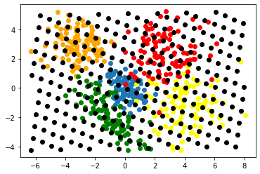
(a) 500 sample points and 256 potential representative points

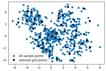
(b) Mixed-Integer Solver (Gurobi with a Python extension)

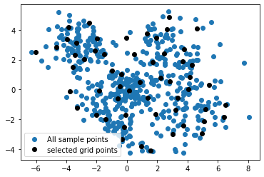
(c) Subgradient method with momentum

Figure 1: $\text{dim}(\beta)=128000$, $\text{dim}(\gamma)=256$, and 51 selected particles.

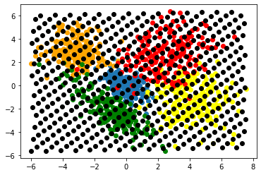
(a) 1000 sample points and 512 potential representative points

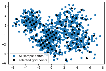
(b) Mixed-Integer Solver (Gurobi with a Python extension)

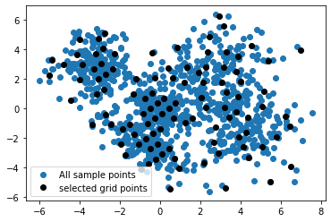
(c) Subgradient method with momentum

Figure 2: $\text{dim}(\beta)=512000$, $\text{dim}(\gamma)=512$, and 102 selected particles

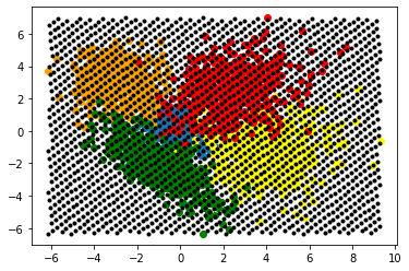
(a) 2500 sample points and 2048 potential representative points

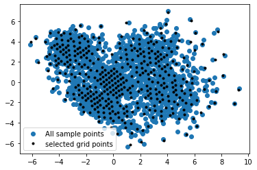
(b) Mixed-Integer Solver (Gurobi with a Python extension)

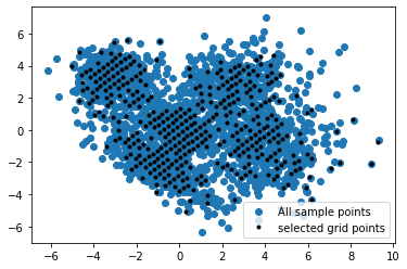
(c) Subgradient method with momentum

Figure 3: $\text{dim}(\beta)=5120000$, $\text{dim}(\gamma)=2048$, and 409 selected particles

Table 2: Grid point selection with the subgradient method on multivariate Gaussian distribution

dim	dim($\beta$)	dim($\gamma$)	subgradient (s)	subgradient $W_{1}$	duality gap
3	20000000	4000	2661	0.361	0.01208
4	31500000	4500	19493	0.564	0.00109
5	40000000	5000	11922	0.830	0.00388

5 Conclusion

The integrated transportation distance provides possibilities to approximate a large-scale Markov system with a simpler system and a finite state space. Based on this distance metric, we proposed a novel particle selection method that iteratively approximates the forward system stage-by-stage by utilizing our kernel distance. The heart of the method is a decomposable and parallelizable subgradient algorithm for particle selection, designed to circumvent the complexities of dealing with constraints and matrix computations.

To empirically validate our approach, we provide a straightforward example involving a 2-dimensional and 1-time-stage Gaussian distribution. We selected this simple case to aid in visualizing outcomes, enabling effective method comparisons and highlighting the limitations of Mixed Integer Programming (MIP) solvers in more complicated scenarios.

Additionally, it’s worth noting that the integrated transportation distance and the particle selection method hold significant potential for various applications, especially with the aid of the dual subbgradient method. One such application pertains to look-ahead risk assessment in reinforcement learning, specifically in the context of Markov risk measures. Evaluating Markov risk measures in dynamic systems can be achieved through the equation (2), offering superior performance over one-step look-ahead methods. This approach streamlines risk or reward evaluation across a range of scenarios by substituting the approximate kernel in place of the original equation (2). We intend to explore the full spectrum of potential applications for this work in future research endeavors.

References

- [1] J. Altschuler, J. Niles-Weed, and P. Rigollet. Near-linear time approximation algorithms for optimal transport via Sinkhorn iteration. In I. Guyon, U. V. Luxburg, S. Bengio, H. Wallach, R. Fergus, S. Vishwanathan, and R. Garnett, editors, Advances in Neural Information Processing Systems, volume 30. Curran Associates, Inc., 2017.
- [2] M. Arjovsky, S. Chintala, and L. Bottou. Wasserstein GAN, 2017. arXiv:1701.07875.
- [3] X. Bing, F. Bunea, and J. Niles-Weed. The sketched Wasserstein distance for mixture distributions, 2022. arXiv:2206.12768.
- [4] Y. Chen, J. Ye, and J. Li. Aggregated Wasserstein distance and state registration for hidden Markov models. IEEE Transactions on Pattern Analysis and Machine Intelligence, 42(9):2133–2147, 2020.
- [5] M. Cuturi. Sinkhorn distances: Lightspeed computation of optimal transport. In C. Burges, L. Bottou, M. Welling, Z. Ghahramani, and K. Weinberger, editors, Advances in Neural Information Processing Systems, volume 26. Curran Associates, Inc., 2013.
- [6] M. Cuturi and G. Peyré. A smoothed dual approach for variational Wasserstein problems. SIAM Journal on Imaging Sciences, 9(1):320–343, 2016.
- [7] M. Cuturi and G. Peyré. Semidual regularized optimal transport. SIAM Review, 60(4):941–965, 2018.
- [8] J. Delon and A. Desolneux. A Wasserstein-type distance in the space of Gaussian mixture models. SIAM Journal on Imaging Sciences, 13(2):936–970, 2020.
- [9] S. Dereich, M. Scheutzow, and R. Schottstedt. Constructive quantization: Approximation by empirical measures. Annales de l’IHP Probabilités et Statistiques, 49(4):1183–1203, 2013.
- [10] P. Dvurechenskii, D. Dvinskikh, A. Gasnikov, C. Uribe, and A. Nedich. Decentralize and randomize: Faster algorithm for Wasserstein barycenters. In S. Bengio, H. Wallach, H. Larochelle, K. Grauman, N. Cesa-Bianchi, and R. Garnett, editors, Advances in Neural Information Processing Systems, volume 31. Curran Associates, Inc., 2018.
- [11] P. Dvurechensky, A. Gasnikov, and A. Kroshnin. Computational optimal transport: Complexity by accelerated gradient descent is better than by Sinkhorn’s algorithm. In J. Dy and A. Krause, editors, Proceedings of the 35th International Conference on Machine Learning, volume 80 of Proceedings of Machine Learning Research, pages 1367–1376. PMLR, 10–15 Jul 2018.
- [12] N. Fournier and A. Guillin. On the rate of convergence in Wasserstein distance of the empirical measure. Probability Theory and Related Fields, 162(3):707–738, 2015.
- [13] G. Garrigos and R. M. Gower. Handbook of convergence theorems for (stochastic) gradient methods, 2023. arXiv:2301.11235.
- [14] A. Genevay, M. Cuturi, G. Peyré, and F. Bach. Stochastic optimization for large-scale optimal transport. In Proceedings of the 30th International Conference on Neural Information Processing Systems, NIPS’16, page 3440–3448, Red Hook, NY, USA, 2016. Curran Associates Inc.
- [15] H. Heitsch and W. Römisch. Scenario tree modeling for multistage stochastic programs. Mathematical Programming, 118(2):371–406, 2009.
- [16] N. Ho, X. Nguyen, M. Yurochkin, H. H. Bui, V. Huynh, and D. Phung. Multilevel clustering via Wasserstein means, 2017. arXiv:1706.03883.
- [17] K. Høyland and S. W. Wallace. Generating scenario trees for multistage decision problems. Management Science, 47(2):295–307, 2001.
- [18] M. Kaut and S. W. Wallace. Shape-based scenario generation using copulas. Computational Management Science, 8(1):181–199, 2011.
- [19] S. Kolouri, G. K. Rohde, and H. Hoffmann. Sliced Wasserstein distance for learning Gaussian mixture models. In Proceedings of the IEEE Conference on Computer Vision and Pattern Recognition (CVPR), June 2018.
- [20] A. Kroshnin, N. Tupitsa, D. Dvinskikh, P. Dvurechensky, A. Gasnikov, and C. Uribe. On the complexity of approximating Wasserstein barycenters. In K. Chaudhuri and R. Salakhutdinov, editors, Proceedings of the 36th International Conference on Machine Learning, volume 97 of Proceedings of Machine Learning Research, pages 3530–3540. PMLR, 09–15 Jun 2019.
- [21] T. Larsson, M. Patriksson, and A.-B. Strömberg. Ergodic, primal convergence in dual subgradient schemes for convex programming. Mathematical Programming, 86:283–312, 1999.
- [22] T. Lin, N. Ho, and M. Jordan. On efficient optimal transport: An analysis of greedy and accelerated mirror descent algorithms. In K. Chaudhuri and R. Salakhutdinov, editors, Proceedings of the 36th International Conference on Machine Learning, volume 97 of Proceedings of Machine Learning Research, pages 3982–3991. PMLR, 09–15 Jun 2019.
- [23] Z. Lin and A. Ruszczyński. An integrated transportation distance between kernels and approximate dynamic risk evaluation in Markov systems, 2023. arXiv:2311.06645.
- [24] Y. Liu, Y. Gao, and W. Yin. An improved analysis of stochastic gradient descent with momentum. Advances in Neural Information Processing Systems, 33:18261–18271, 2020.
- [25] O. Pele and M. Werman. Fast and robust earth mover’s distances. In 2009 IEEE 12th International Conference on Computer Vision, pages 460–467, 2009.
- [26] G. C. Pflug. Version-independence and nested distributions in multistage stochastic optimization. SIAM Journal on Optimization, 20(3):1406–1420, 2010.
- [27] G. C. Pflug and A. Pichler. Dynamic generation of scenario trees. Computational Optimization and Applications, 62(3):641–668, 2015.
- [28] S. T. Rachev and L. Rüschendorf. Mass Transportation Problems: Volume I: Theory. Springer Science & Business Media, 1998.
- [29] Y. Rubner, C. Tomasi, and L. J. Guibas. The earth mover’s distance as a metric for image retrieval. International Journal of Computer Vision, 40:99–121, 2000.
- [30] J. Solomon, R. Rustamov, L. Guibas, and A. Butscher. Wasserstein propagation for semi-supervised learning. In E. P. Xing and T. Jebara, editors, Proceedings of the 31st International Conference on Machine Learning, volume 32 of Proceedings of Machine Learning Research, pages 306–314, Bejing, China, 22–24 Jun 2014. PMLR.
- [31] C. Villani. Optimal Transport: Old and New. Springer, 2009.
- [32] Y. Yan, T. Yang, Z. Li, Q. Lin, and Y. Yang. A unified analysis of stochastic momentum methods for deep learning. In Proceedings of the 27th International Joint Conference on Artificial Intelligence, pages 2955–2961, 2018.
- [33] M. Zinkevich. Online convex programming and generalized infinitesimal gradient ascent. In Proceedings of the 20th International Conference on Machine Learning (ICML-03), pages 928–936, 2003.