Bayesian inference on Cox regression models using catalytic prior distributions

Abstract

The Cox proportional hazards model (Cox model) is a popular model for survival data analysis. When the sample size is small relative to the dimension of the model, the standard maximum partial likelihood inference is often problematic. In this work, we propose the Cox catalytic prior distributions for Bayesian inference on Cox models, which is an extension of a general class of prior distributions originally designed for stabilizing complex parametric models. The Cox catalytic prior is formulated as a weighted likelihood of the regression coefficients based on synthetic data and a surrogate baseline hazard constant. This surrogate hazard can be either provided by the user or estimated from the data, and the synthetic data are generated from the predictive distribution of a fitted simpler model. For point estimation, we derive an approximation of the marginal posterior mode, which can be computed conveniently as a regularized log partial likelihood estimator. We prove that our prior distribution is proper and the resulting estimator is consistent under mild conditions. In simulation studies, our proposed method outperforms standard maximum partial likelihood inference and is on par with existing shrinkage methods. We further illustrate the application of our method to a real dataset.

Keywords Prior specification  $\cdot$ proportional hazards model  $\cdot$ synthetic data  $\cdot$ stable estimation  $\cdot$ regularization

1 Introduction

Survival analysis plays a pivotal role in various fields, such as medicine, public health, genetics, and engineering (Mills, 2010; Kalbfleisch & Prentice, 2011; Latimer, 2013). Understanding the relationship between survival time (time-to-event data) and risk factors is vital in such analyses. The well-known Cox proportional hazards model (Cox model) (Cox, 1972) is the most frequently used tool for investigating this relationship. This model assumes a proportional hazards structure and is composed of two parts: a nonparametric baseline hazards function and a parametric component that contains regression coefficients for covariates. The parametric component elucidates the association between risk factors and hazards, and is thus often the main focus for researchers.

Existing estimation methods for the parametric component in the Cox model are not fully satisfactory when the number of observations is not sufficiently large relative to the number of covariates, a situation often seen in clinical studies and other survival analyses (Beca et al., 2021). The current paper studies the Bayesian inference for the Cox model and we aim to propose a class of prior distributions that are able to provide stable Bayesian inference even when the sample size is not sufficiently large. Throughout the paper, we use the compact term “priors" in place of the long term “prior distributions" for convenience.

A standard frequentist’s estimation method for the Cox model is the maximum partial likelihood estimator (MPLE) (Cox, 1972, 1975), which focuses on the parametric component and does not involve the estimation of the baseline hazard function. The MPLE has been widely used in practical applications due to the availability of easy-to-use software (Therneau & Grambsch, 2000). For any fixed Cox model, theoretical properties of the MPLE have been well-developed (Tsiatis, 1981; Andersen & Gill, 1982; Wong, 1986). However, when the dimension $p$ of the model is comparable to or larger than $n$, the MPLE is unstable and biased (Bryson & Johnson, 1981; Zhang et al., 2022). Such problematic behaviors of MPLE demand careful consideration.

Bayesian estimation offers a general alternative to the MPLE in small samples. However, its application to the Cox model faces several challenges, especially in choosing the prior. In the cases where the MPLE fails, using a simple flat prior may not result in a well-behaved posterior. In addition, the commonly used parametric families, such as normal distributions or Cauchy distributions, require a subjective choice of hyper-parameters, which could be difficult to justify and interpret. Furthermore, the Jeffreys prior may not exist (Wu et al., 2018), or its implementation may be computationally intensive due to its numerical evaluation of the Hessian matrix. Although informative priors, such as the power priors (Ibrahim & Chen, 1998), are beneficial in incorporating addition information or historical data (Neuenschwander et al., 2010), their applicability are limited to certain contexts (Brard et al., 2017; van Rosmalen et al., 2018).

To address these challenges in applying Bayesian estimation to the Cox model, particularly in prior specification and computational feasibility, we consider the adaption of a recently proposed class of automatic priors called “catalytic priors" (Huang et al., 2020). A catalytic prior is designed to stabilize a high-dimensional parametric model by supplementing the observed data with a small amount of synthetic data generated from the predictive distribution based on a simpler model. Such a prior is formulated as a fractional exponent of the likelihood based on the synthetic data. This strategy enhances the stability and reliability of the estimation process, especially in situations where the samples size is small relative to the dimension of the model.

Although the class of catalytic priors has been demonstrated successful in providing superior performance in finite-sample inference in generalized linear models with dimensions close to the sample sizes, the original proposal in Huang et al. (2020) focuses on parametric models. It does not apply to Cox models for survival analysis due to the non-parametric components. It is of our main focus to extend the original idea of catalytic priors to Cox models so that the new class of priors inherits the benefits for Bayesian inference in small samples.

1.1 Summary and outline

In this paper, we extend the catalytic prior method to Cox models. This method ensures stable estimation of the regression coefficients, which is particularly useful when the sample size is not large relative to the dimension of the model. The main contributions are summarized as follows:

1. We introduce a new class of priors, call Cox catalytic priors, for the coefficients in the semi-parametric Cox model, which can be seamlessly integrated with any existing Bayesian samplers tailored to the posterior inference for the Cox model. We prove that this prior is proper under mild assumptions, a necessary property for for many Bayesian inferences, such as model comparison using the Bayes factor.

2. We introduce a regularized estimator based on the marginal posterior distribution of the coefficients, which can be efficiently computed using any convex optimization software since the objective optimization function is strongly convex. Furthermore, we theoretically establish the consistency of this regularized estimator.

3. We utilize synthetic data to define a simultaneous prior on both the coefficients and the baseline hazard function. This prior leads to a point estimator of the coefficients, which can be easily computed using existing software designed for the Cox model.

Through simulation studies, we demonstrate that our proposed estimation methods outperform the classical maximum partial likelihood estimation in the challenging situations where the sample size is not sufficiently large relative to the dimension of covariates. Furthermore, their performance is comparable and sometimes superior to existing regularized methods.

The remainder of the paper is structured as follows. In Section 2, we briefly review the catalytic prior and the Cox model. In Section 3, we introduce the construction of Cox catalytic priors for Cox models and propose two estimation methods based on these priors. We establish some theoretical guarantees for the proposed priors and estimators in Section 4. The numerical performance of our proposed methods is examined via simulations in Section 5. In Section 6, we apply these methods to a real-world dataset. Finally, Section 7 concludes the article with a discussion.

1.2 Related literature

Our work is related to three areas of research: (1) specification of prior distributions, (2) regularizied estimations, and (3) survival models.

The use of synthetic data for constructing prior distributions has a long-standing tradition in Bayesian statistics (Good, 1983). It’s recognized that conjugate priors for exponential families can be interpreted as the likelihood of pseudo-observations (Raiffa et al., 1961). Although there are prior formulations that incorporate additional synthetic data from experts’ knowledge (Bedrick et al., 1996, 1997), they often encounter challenges during practical implementation, especially with high-dimensional data or when considering multiple models. For addressing challenges in Bayesian model selection, a promising alternative is the class of the expected-posterior priors (Iwaki, 1997; Pérez & Berger, 2002; Neal, 2001), where a prior is defined as the average posterior distribution derived from a set of synthetic data sampled from a straightforward predictive model. Wu et al. (2018) proposed Jeffreys-type priors to to deal with the monotone partial likelihood problem in Cox models. Informative priors, such as the power priors (Ibrahim & Chen, 2000; Chen et al., 2000; Ibrahim & Chen, 1998), effectively incorporate information from historical data using a power of the likelihood function of those data. However, the validity of a power prior mandates that the covariate matrix of historical data has full column rank, which may fail to hold. In addition, historical data might not always be available. In contrast, the catalytic prior is based on synthetic data sampled from a simpler model, which serve as a replacement for historical data.

Apart from the Bayesian strategies, regularized partial likelihood methods are also employed to stabilize high-dimensional Cox models. In particular, the $\ell_{2}$-regularizer is frequently used in practice to shrink regression coefficients towards smaller values, which is often referred to as Ridge regression (Hoerl & Kennard, 1970). (Verweij & Van Houwelingen, 1993) adopted the $\ell_{2}$-penalty to regularize the negative log partial likelihood, and (Huang & Harrington, 2002) demonstrated that Ridge regression can yield a lower mean square error and improved prediction accuracy of relative risk compared to the MPLE, especially in small samples. (Bøvelstad et al., 2007) compared the prediction performance resulting from different estimation, where Ridge regression demonstrated the best overall performance for their microarray gene expression datasets.

Although this paper focus on the proportional hazards model, there are many other semiparametric survival models (Aalen, 1989; Wei, 1992; Murphy et al., 1997). We refer the interested reader to Hanson & Jara (2013) for a review and to the monograph Ibrahim et al. (2001) for a comprehensive treatment of Bayesian survival analysis.

2 Review of existing methods

This section provides a succinct introduction to the Cox model, the MPLE and its variants, and the original catalytic prior method for parametric models.

2.1 Proportional hazards model and partial likelihood

For a given subject $i$, denoted by $T_{i}$ the survival time which may be right censored by a censoring time $C_{i}$. The observed data is represented by a triplet $\left(\boldsymbol{X}_{i},Y_{i},\delta_{i}\right)$, where $\boldsymbol{X}_{i}\in\mathbb{R}^{p}$ is the covariate vector, $\delta_{i}$ is the binary event indicator, and $Y_{i}$ is the observed time, satisfying that $\delta_{i}=\mathbf{1}[T_{i}\leq C_{i}]$ and $Y_{i}=\min(T_{i},C_{i})$. We assume censoring is non-informative, i.e., $T_{i}\perp C_{i}\mid\boldsymbol{X}_{i}$.

In the Cox model, the hazard for subject $i$ at time $t$ has the form $h(t\mid\boldsymbol{X_{i}})=h_{0}(t)\exp\left(\boldsymbol{X}_{i}^{\prime}\boldsymbol{\beta}\right)$, where $h_{0}(\cdot)$ is a unknown baseline hazard function and it is a nuisance parameter for our study. The likelihood is given as:

$$L\left(\boldsymbol{\beta},h_{0}\mid\left\{\left(\boldsymbol{X}_{i},Y_{i},\delta_{i}\right)\right\}_{i=1}^{n}\right)=\prod_{i=1}^{n}\left\{\exp\left(\boldsymbol{X}_{i}^{\prime}\boldsymbol{\beta}\right)h_{0}\left(Y_{i}\right)\right\}^{\delta_{i}}\exp\left\{-\exp\left(\boldsymbol{X}_{i}^{\prime}\boldsymbol{\beta}\right)H_{0}\left(Y_{i}\right)\right\},$$ (1)

where $H_{0}(t)=\int_{0}^{t}h_{0}(u)du$ is the cumulative baseline hazard function. To estimate $\boldsymbol{\beta}$, Cox (1975) proposed using the partial likelihood to estimate the parametric components without considering the baseline hazard. Given $n$ independent subjects $\left\{\left(\boldsymbol{X}_{i},Y_{i},\delta_{i}\right)\right\}_{i=1}^{n}$, the partial likelihood of $\boldsymbol{\beta}$ is formulated as follows:

$$PL(\boldsymbol{\beta})=\prod_{i=1}^{n}\left\{\frac{\exp\left(\boldsymbol{X}_{i}^{\prime}\boldsymbol{\beta}\right)}{\sum_{j\in\mathbf{R}_{i}}\exp\left(\boldsymbol{X}_{j}^{\prime}\boldsymbol{\beta}\right)}\right\}^{\delta_{i}}$$ (2)

where $\mathbf{R}_{i}:=\{j:Y_{j}\geq Y_{i}\}$ is the collection of subjects who are at risk at time $Y_{i}$. The estimator obtained by maximizing (2) is also referred to as MPLE, when the context is clear. This estimator can be efficiently determined using the Newton-Raphson method. Regularization of MPLE can be achieved by adding the $\ell_{1}$-penalty (Tibshirani, 1997) or the $\ell_{2}$-penalty (Hoerl & Kennard, 1970) to the negative log partial likelihood. These regularization methods correspond to Lasso and Ridge, respectively. We shall investigate the performance of these two approaches in our simulation.

When the number of covariates $p$ is fixed and the sample size $n$ is large, asymptotic properties of the MPLE have been extensively studied in the literature (Tsiatis, 1981; Andersen & Gill, 1982; Wong, 1986; Murphy & Van der Vaart, 2000). When $n$ is small, however, the MPLE is known to be unstable and some of the estimates may diverge to infinity (Bryson & Johnson, 1981). In addition, when $n$ is large but $p$ scales with $n$, the estimated coefficients may have exaggerated magnitudes, leading to a bias away from zero (Zhang et al., 2022). In the supplementary material A.5, we reproduce a simple simulation in Zhang et al. (2022) to illustrate the biased behavior of the MPLE when the dimension is large. The unstable and biased behaviors of the MPLE in large dimensions necessitate alternative estimation methods.

2.2 Catalytic prior: specification and property

The motivation behind the catalytic prior is the understanding that data are real while models are imperfect tools designed to analyze data. From this data-centric perspective, specifying a prior distribution is analogous to adding some hypothetical “prior data" to the observed data, which will be elaborated in the following review.

Let $\left\{\left(Y_{i},\boldsymbol{X}_{i}\right)\right\}_{i=1}^{n}$ be $n$ independent pairs of observed data, where $Y_{i}$ is a response and $\boldsymbol{X}_{i}$ is a covariate vector. Suppose the goal is to use $\left\{\left(Y_{i},\boldsymbol{X}_{i}\right)\right\}_{i=1}^{n}$ to fit a complex (e.g., large dimensional) target model for $Y_{i}$ given $\boldsymbol{X}_{i}$ that assumes the observations are drawn as follows:

$$Y_{i}\mid\boldsymbol{X}_{i},\boldsymbol{\theta}\sim f\left(y\mid\boldsymbol{X}_{i},\boldsymbol{\theta}\right),i=1,2\ldots,n,$$ (3)

where $f$ is corresponding probability density function, $\boldsymbol{\theta}$ is the unknown target parameter that is hard to estimate using the small sample.

The basic idea of catalytic priors is to generate synthetic data from a simpler model, and use the synthetic data as prior information for fitting the complex target model $f$. Suppose a simpler model $g(y\mid\boldsymbol{X},\boldsymbol{\psi})$ with unknown parameter $\boldsymbol{\psi}$ is stably fitted from $\left\{\left(Y_{i},\boldsymbol{X}_{i}\right)\right\}_{i=1}^{n}$ and results in a synthetic data-generating distribution $g_{*}(y\mid\boldsymbol{x},\left\{\left(Y_{i},\boldsymbol{X}_{i}\right)\right\}_{i=1}^{n})$. Then $M$ synthetic data points $\left\{\left(Y_{i}^{*},\boldsymbol{X}_{i}^{*}\right)\right\}_{i=1}^{M}$ can be generated as follows:

$$\boldsymbol{X}_{i}^{*}\stackrel{{\scriptstyle i.i.d.}}{{\sim}}Q(\boldsymbol{x}),\quad Y_{i}^{*}\mid\boldsymbol{X}_{i}^{*}\sim g_{*}\left(y\mid\boldsymbol{X}_{i}^{*},\left\{\left(Y_{i},\boldsymbol{X}_{i}\right)\right\}_{i=1}^{n}\right),$$ (4)

where $Q$ denotes the distribution from which the synthetic covariates $\boldsymbol{X}^{*}$ are generated. Huang et al. (2020) discussed various strategies to generate synthetic data. Since synthetic data is not real data, and we reduce the impact of synthetic data by down-weighting with a positive tuning parameter $\tau$ which determines their total weight – intuitively, the total weight of the synthetic data corresponds to $\tau$ data points, each with weight $\tau/M$. In particular, the catalytic prior is defined as

$$\pi_{cat,M}(\boldsymbol{\theta}\mid\tau)\propto\left\{\prod_{i=1}^{M}f\left(Y_{i}^{*}\mid\boldsymbol{X}_{i}^{*},\boldsymbol{\theta}\right)\right\}^{\frac{\tau}{M}}=\exp\left\{\frac{\tau}{M}\sum_{i=1}^{M}\log\left(f\left(Y_{i}^{*}\mid\boldsymbol{X}_{i}^{*},\boldsymbol{\theta}\right)\right)\right\}$$ (5)

We can treat catalytic prior as a down-weighted version of likelihood based on synthetic data. Based on (5), the posterior distribution can be written as

$$\pi(\boldsymbol{\theta}\mid\left\{\left(Y_{i},\boldsymbol{X}_{i}\right)\right\}_{i=1}^{n}) \propto\left(\prod_{i}^{n}f(Y_{i}\mid\boldsymbol{X}_{i},\boldsymbol{\theta})\right)\pi_{cat,M}(\boldsymbol{\theta}\mid\tau)$$ (6)

$$\propto\exp\left\{\sum_{i=1}^{n}\log\left(f\left(Y_{i}\mid\boldsymbol{X}_{i},\boldsymbol{\theta}\right)\right)+\frac{\tau}{M}\sum_{i=1}^{M}\log\left(f\left(Y_{i}^{*}\mid\boldsymbol{X}_{i}^{*},\boldsymbol{\theta}\right)\right)\right\}.$$

Being data-dependent, this construction can be viewed as an empirical Bayes method, which may be traced back to the classical Box-Cox transformation (Box & Cox, 1964).

This class of prior offers several significant benefits. Firstly, since the posterior has the same form as the likelihood, Bayesian inference based on the posterior is no more difficult than any likelihood-based inference. For example, the posterior mode can be conveniently computed as the maximum weighted likelihood estimate using standard statistical software. Secondly, unlike some other priors such as Gaussian prior or Cauchy priors, this class does not focus on the parameter space, adding to its robustness to the choice of model parametrization. Furthermore, it allows for easy interpretation of the information included by the prior through the use of synthetic data. Lastly, this class of prior is generic and applicable to any parametric models, making it a versatile tool in various applications of Bayesian methods.

3 Catalytic prior distributions for Cox models

The catalytic prior distribution mentioned in Section 2.2 can only work for a parametric model. In this study, we consider the semi-parametric Cox model, and our interest lies in the inference on the regression parameter $\boldsymbol{\beta}$. Due to the existence of an unknown nuisance component $h_{0}(\cdot)$, we cannot write down the catalytic prior for $\boldsymbol{\beta}$ directly from the likelihood function (1). In this section, we propose a new catalytic prior for the regression coefficient $\boldsymbol{\beta}$ in the Cox model with application to Bayesian inference. We also derive the corresponding point estimator and discuss an alternative construction of the catalytic prior on both coefficients and baseline hazard function.

3.1 Prior formulation

To begin with, suppose synthetic data are given and denoted by $\left\{\left(\boldsymbol{X}_{i}^{*},Y_{i}^{*}\right)\right\}_{i=1}^{M}$, where $\boldsymbol{X}_{i}^{*}$ is a synthetic covariate vector, $Y_{i}^{*}$ is a synthetic survival time. Unlike the observed data, there is no censoring in these synthetic data since we have full control on their generation. For the Cox model in (1), the likelihood derived from the synthetic data will depend only on the coefficient $\boldsymbol{\beta}$ if we substitute the nuisance component by a simple user-specific baseline hazard constant $h^{+}_{0}$. This substitution leads us to define the Cox catalytic prior for $\boldsymbol{\beta}$ as follows:

$$\pi_{cox,cat}(\boldsymbol{\beta}\mid\tau)\propto L\left(\boldsymbol{\beta},h_{0}^{+}\mid\left\{\left(\boldsymbol{X}_{i}^{*},Y_{i}^{*}\right)\right\}_{i=1}^{M}\right)^{\tau/M}$$ (7)

$$= \left[\prod_{i=1}^{M}\left\{\exp\left(\boldsymbol{X}_{i}^{*\prime}\boldsymbol{\beta}\right)h_{0}^{+}\right\}\exp\left\{-\exp\left(\boldsymbol{X}_{i}^{*\prime}\boldsymbol{\beta}\right)Y_{i}^{*}h^{+}_{0}\right\}\right]^{\tau/M},$$

where $h^{+}_{0}$ and $\tau$ are positive constants. Notably, the scalar $h_{0}^{+}$ acts merely as a surrogate for the nuisance component to facilitate the construction of our catalytic prior. It does not need to be correctly specified or unbiased. In practice, it can be specified by the user or computed in a data driven way.

The separable form of the Cox catalytic prior enables us to evaluate it efficiently. Furthermore, one can see that the Cox catalytic prior is log-concave, so its tails are typically well-behaved. The log-concavity of the Cox catalytic prior will also be useful in the posterior sampling, if the likelihood function is log-concave in $\boldsymbol{\beta}$ (fixing $h$); we provide an example in Section A.2 where the update step of $\boldsymbol{\beta}$ in a Gibbs iteration involves a log-concave distribution, from which efficient sampling is possible (Lovász & Vempala, 2006). For a comprehensive review on log-concave densities, see (Saumard & Wellner, 2014). In addition, we prove in Section 4 that the Cox catalytic prior is proper under some mild conditions.

The Cox catalytic prior in (7) offers a compelling alternative to the default prior for $\boldsymbol{\beta}$ in the standard Bayesian Cox model. This alternative is not only simple to implement but also provides easy interpretation through the use of synthetic data.

3.2 Specification of components

To specify the Cox catalytic prior defined in Section 3.1, one need to generate synthetic survival data and choose the values of $M$ and $\tau$.

Similarly to the introduction in Section 2.2, the procedure for generating the synthetic survival data $\left\{\left(\boldsymbol{X}_{i}^{*},Y_{i}^{*}\right)\right\}_{i=1}^{M}$ can be summarized as:

1. Synthetic covariates: Use any appropriate methods in (Huang et al., 2020) to generate $\left\{\boldsymbol{X}_{i}^{*}\right\}_{i=1}^{M}$. For example, each coordinate $\boldsymbol{X}_{i,j}^{*}$ is independently resampled from the corresponding $j$-th marginal empirical distribution of the observed covariates.

2. Synthetic survival time: Consider a simpler model $g(y\mid\boldsymbol{X},\boldsymbol{\delta},\boldsymbol{\psi})$ with an unknown parameter $\boldsymbol{\psi}$, where $\boldsymbol{\psi}$ is low-dimensional and the model can be stably fitted from the observed data $\left\{\left(\boldsymbol{X}_{i},Y_{i},\delta_{i}\right)\right\}_{i=1}^{n}$. Using either a point estimate or a Bayesian posterior, one can obtain a predictive distribution from this simpler model, denoted by $g_{*}(y\mid\boldsymbol{x},\left\{\left(\boldsymbol{X}_{i},Y_{i},\delta_{i}\right)\right\}_{i=1}^{n})$. Then synthetic survival time can be generated according to $Y_{i}^{*}\mid\boldsymbol{X}_{i}^{*}\sim g_{*}\left(y\mid\boldsymbol{X}_{i}^{*},\delta_{i}^{*}=1,\left\{\left(\boldsymbol{X}_{i},Y_{i},\delta_{i}\right)\right\}_{i=1}^{n}\right)$, where $\delta_{i}^{*}=1$ denotes the uncensored status of the synthetic unit.

There are plenty of choices for the simpler models $g(y\mid\boldsymbol{X},\boldsymbol{\delta},\boldsymbol{\psi})$. For example, one could use a parametric survival model for the survival time $T$ using exponential distributions or Weibull distributions. Alternatively, one could use a nonparametric model for the survival function without using any covariates and fit it via the Kaplan-Meier estimator.

As a simple example, we generate synthetic survival times from an estimated exponential distribution, i.e., $Y_{i}^{*}\sim\text{Exp}(\hat{\psi})$, where $\hat{\psi}$ is estimated stably based on the observed data by maximizing following the likelihood function of $\psi$:

$$L\left(\psi\mid\left\{\left(\boldsymbol{X}_{i},Y_{i},\delta_{i}\right)\right\}_{i=1}^{n}\right)=\prod_{i=1}^{n}\psi^{\delta_{i}}\exp\left\{-\psi Y_{i}\right\},\quad\psi>0.$$ (8)

This likelihood corresponds to a simple nested model of (1), where the model parameters are restricted to be $\boldsymbol{\beta}=0$ and $h_{0}(t)=\psi$ for all $t>0$. The estimate $\hat{\psi}$ can also be used to specify the surrogate $h_{0}^{+}=\hat{\psi}$ when we construct the Cox catalytic prior for $\boldsymbol{\beta}$.

The synthetic sample size $M$, in general, should be as large as possible, but in practice the returns vanish when $M$ exceeds a certain point. Without a universal value of $M$ that suits all problems, we advise the users to experiment with different values of $M$ based on the scale of their specific problem and available computational resources. To ensure the properness of the catalytic prior for Cox regression with $p$ covariates, we also recommend that $M$ is at least $4p$ based on the theory in Section 4.

The total weight $\tau$ is an important hyperparameter because it controls the influence of the catalytic prior on the posterior inference. A simple but useful choice is to set $\tau$ equal to $p$, the dimension of $\boldsymbol{\beta}$ (Huang et al., 2022). Alternatively, we can adopt frequentist methods to fine-tune $\tau$ by optimizing a given criteria function, such as the cross-validated partial log-likelihood outlined in the supplementary material.

If a fully Bayesian perspective on $\tau$ is adopted, we can impose a joint prior on $(\tau,\beta)$ so that the tuning parameter $\tau$ is adaptively specified by the data. Given any two positive scalar hyperparameters $\alpha$ and $\gamma$, we define the Cox adaptive catalytic prior for $(\tau,\boldsymbol{\beta})$ as

$$\pi_{\alpha,\gamma}(\tau,\boldsymbol{\beta})\propto\Gamma_{\alpha,\gamma}(\tau)\cdot L\left(\boldsymbol{\beta},h_{0}^{+}\mid\left\{\left(\boldsymbol{X}_{i}^{*},Y_{i}^{*}\right)\right\}_{i=1}^{M}\right)^{\tau/M}$$ (9)

where $\Gamma_{\alpha,\gamma}(\tau)$ is a function defined as

$$\Gamma_{\alpha,\gamma}(\tau)=\tau^{p+\alpha-1}e^{-\tau\left(\kappa+\gamma^{-1}\right)}$$ (10)

and

$$\kappa:=\sup_{\boldsymbol{\beta}\in\mathbb{R}^{p}}\frac{1}{M}\log L\left(\boldsymbol{\beta},h_{0}^{+}\mid\left\{\left(\boldsymbol{X}_{i}^{*},Y_{i}^{*}\right)\right\}_{i=1}^{M}\right)$$ (11)

The form of $\Gamma_{\alpha,\gamma}(\tau)$ is chosen in this way such that the conditional posterior of $\tau$ given $\beta$ is a Gamma distribution, which is easier to sample from. This simplifies the update step of $\tau$ in the iteration of the Gibbs algorithm. Furthermore, Theorem 2 shows that the Cox adaptive catalytic prior is proper. The hyperparameters $\alpha$ and $\gamma$ control the tail behavior of $\tau$ in this joint prior; a larger value of $\alpha$ (or $\gamma$) tends to pull the working model more towards the simpler model. The values of $\alpha$ and $\gamma$ are chosen by the user, and there does not exist a single choice of $(\alpha,\gamma)$ that works the best in all scenarios. In our numerical experiments, we observed that the choice of $(\alpha,\gamma)=(2,1)$ works well.

3.3 Bayesian inference and approximate MAP estimator

The full Bayesian analysis of a Cox model using a catalytic prior in (7) can be conducted using standard techniques such as posterior sampling. This usually involves placing a nonparametric prior process to model the baseline hazard $h_{0}(t)$ and deriving the joint posterior of $(\boldsymbol{\beta},h_{0})$. Monte Carlo methods for Bayesian inference on Cox models has been well-established in the literature; see for example, Chen et al. (2012). We provide a detailed description of the full Bayesian inference using the Cox catalytic prior and a Gamma process for modeling the cumulative hazard function in Section A.1 in the supplementary material. Source code for implementing the posterior sampling using R and Stan, which are popular open-source software and interfaces for conducting Bayesian analysis, can be found in the supplementary material.

After from inference based on posterior distribution, when point estimation is of the primary interest, maximum a posteriori (MAP) estimation is often favored. The MAP estimate is equal to the mode of the posterior distribution, and it is often much simpler to compute than other posterior estimates, especially when sampling from the posterior distribution is difficult. This is particularly the case for Cox models because the nonparametric baseline hazard function may make the Bayesian computation expensive and time-consuming.

To mitigate the computational burden for the point estimation using the Cox catalytic prior, we consider the following approximation to the mode of the marginal posterior for $\boldsymbol{\beta}$ maximizing the regularized log partial likelihood

$$\hat{\boldsymbol{\beta}}_{CR,\tau}=\arg\max_{\boldsymbol{\beta}}\left\{\log PL(\boldsymbol{\beta})+\log\pi_{cox,cat}(\boldsymbol{\beta}\mid\tau)\right\},$$ (12)

where the regularization term is the log density of the Cox catalytic prior for $\boldsymbol{\beta}$. For simplicity, we call this estimator $\hat{\boldsymbol{\beta}}_{CR,\tau}$ the catalytic-regularized estimator (CRE) in the rest of the paper. Since both $\log(PL(\boldsymbol{\beta}))$ and $\log(\pi_{cox,cat}(\boldsymbol{\beta}\mid\tau))$ are concave functions with respect to $\boldsymbol{\beta}$, we can adopt any efficient convex optimization method such as Newton-Raphson method to find $\hat{\boldsymbol{\beta}}_{CR,\tau}$.

The justification for using the approximation in (12) is based on the approximation of the marginal posterior of $\boldsymbol{\beta}$ when we place an independent diffused prior on the baseline hazard function. A detailed explanation is provided in Section A.3 in the supplementary material.

3.4 Estimation utilizing synthetic data

In addition to the Cox catalytic prior on $\boldsymbol{\beta}$, we can construct a prior on both the coefficients and the baseline hazard function. This alternative construction will lead to an estimator for $\boldsymbol{\beta}$ that can be intuitively interpreted as estimation based on a combination of the weighted synthetic data and the actual observed data.

In the context of a parametric model, the catalytic prior in Eq. (5) is defined as a down-weighted version of the likelihood based on synthetic data. As a result, the corresponding posterior can be regarded as a “likelihood" based on a mixture of observed data (each with a weight of 1) and synthetic data (each with a weight of $\tau/M$). This perspective on the posterior can be extended to the Cox model. As an analogy, we consider a “posterior distribution" $\tilde{L}$ on both $\boldsymbol{\beta}$ and $h(\cdot)$ whose density (w.r.t. some base measure) can be expressed as the following weighted likelihood function:

$$\tilde{L}(\boldsymbol{\beta},h(\cdot)\mid\boldsymbol{D},\boldsymbol{D}^{*})=L(\boldsymbol{\beta},h(\cdot)\mid\boldsymbol{D})\cdot L(\boldsymbol{\beta},h(\cdot)\mid\boldsymbol{D}^{*})^{\frac{\tau}{M}}$$ (13)

where $\boldsymbol{D}$ denotes the actual data $\{\left(\boldsymbol{X}_{i},Y_{i},\delta_{i}\right)\}_{i=1}^{n}$ , $\boldsymbol{D}^{*}$ denotes the synthetic data $\left\{\left(\boldsymbol{X}_{i}^{*},Y_{i}^{*}\right)\right\}_{i=1}^{M}$, and $L(\cdot)$ is likelihood defined in (1). The posterior in (13) is associated with a prior on $(\boldsymbol{\beta},h(\cdot))$ whose density (w.r.t. the same base measure as before) is $L(\boldsymbol{\beta},h(\cdot)\mid\boldsymbol{D}^{*})^{\frac{\tau}{M}}$. This prior does not assume the independence between $\boldsymbol{\beta}$ and $h(\cdot)$, making it different from most Bayesian inference on Cox models. Although we will not delve into the full Bayesian inference with (13), we can consider the resultant point estimation by leveraging the profile likelihood method for removing the nuisance parameter $h(\cdot)$.

Following the same treatment employed by (Murphy & Van der Vaart, 2000), we reduce the weighted likelihood in (1) to a new partial likelihood denoted by $P\tilde{L}(\boldsymbol{\beta})$:

$$P\tilde{L}(\boldsymbol{\beta})= \prod_{i\in\tilde{\boldsymbol{I}}}\left(\frac{\theta_{i}}{\sum_{j\in\tilde{\mathcal{R}}_{i}}w_{j}\theta_{j}}\right)^{\tilde{\delta}_{i}w_{i}},$$ (14)

where the notation is described as follows:

• The index set $\tilde{\boldsymbol{I}}=\boldsymbol{I}_{D}\bigcup\boldsymbol{I}_{D^{*}}$, where $\boldsymbol{I}_{D}=\{1,2,\ldots,n\}$ is the index set for observed data and $\boldsymbol{I}_{D^{*}}=\{n+1,n+2,\ldots,n+M\}$ is the index set for synthetic data.

• The combination of observed and synthetic data is denoted by $\{\tilde{Y}_{i}\}_{i=1}^{n+M}$, where $\tilde{Y}_{i}=Y_{i}$ if $i\in\boldsymbol{I}_{D}$ and $\tilde{Y}_{i}=Y^{*}_{i-n}$ if $i\in\boldsymbol{I}_{D^{*}}$.

• $\tilde{\mathcal{R}}_{i}$ denotes the set of subjects at risk at time $\tilde{Y}_{i}$, i.e., $\tilde{\mathcal{R}}_{i}=\{j:\tilde{Y}_{j}\geq\tilde{Y}_{i},j\in\tilde{\boldsymbol{I}}\}$.

• Transformation $\theta_{j}=\exp(\boldsymbol{X}_{j}^{\top}\boldsymbol{\beta})$ if $j\in\boldsymbol{I}_{D}$ or $\theta_{j}^{*}=\exp({\boldsymbol{X}_{j-n}^{*}}^{\top}\boldsymbol{\beta})$ if $j\in\boldsymbol{I}_{D^{*}}$.

• The weight is denoted as $w_{i}=1$ if $i\in\boldsymbol{I}_{D}$ or $w_{i}=\tau/M$ if $i\in\boldsymbol{I}_{D^{*}}$.

• The censoring status is denoted as $\tilde{\delta}_{i}=\delta_{i}$ if $i\in\boldsymbol{I}_{D}$ or $\tilde{\delta}_{i}=1$ if $i\in\boldsymbol{I}_{D^{*}}$.

Subsequently, we define the following estimator by maximizing the new partial likelihood:

$$\hat{\boldsymbol{\beta}}_{WM,\tau}=\arg\max_{\boldsymbol{\beta}}P\tilde{L}(\boldsymbol{\beta}).$$ (15)

This estimator $\hat{\boldsymbol{\beta}}_{WM,\tau}$ will be referred to as the weighted mixture estimator (WME), where the subscript WM indicates the weighting and mixing of observed and synthetic data.

Having defined the WME, we now turn to its properties. By a direct calculation of the second order derivative of $\log P\tilde{L}(\boldsymbol{\beta})$, we can verify that it is a strictly concave function, which allows us to compute $\hat{\boldsymbol{\beta}}_{WM,\tau}$ efficiently. In Section A.4, we derive an explicit form for optimization and provide a simple procedure for computing the WME $\hat{\boldsymbol{\beta}}_{WM,\tau}$ using standard software.

Unlike the CRE $\hat{\boldsymbol{\beta}}_{CR,\tau}$ in (12), whose objective function is separable with an additive regularization term, the objective function for the WME $\hat{\boldsymbol{\beta}}_{WM,\tau}$ is not separable. Nonetheless, the WME should still be regarded as a regularized estimator. In particular, if the total weight parameter $\tau$ decays to $0$, the WME becomes the MPLE based solely on the observed data; if $\tau$ diverge to $\infty$, the WME converges to the MPLE based solely on the synthetic data. Another distinction between the CRE and the WME is that the definition of WME only requires the generation of synthetic data and does not depend on the surrogate baseline hazard constant $h_{0}^{+}$. This attribute makes the WME more robust to the prior specification.

4 Theoretical properties

In this section, we first verify the properness of the Cox catalytic prior introduced in Section 3, then we show that our proposed estimators, CRE and WME, are consistent for the true coefficient parameters.

4.1 Properness

Many Bayesian inferences, such as model comparison using Bayes factors, require a proper prior. To establish the properness of Cox catalytic prior proposed in Section 3.1, we start with a mild assumption regarding synthetic covariates.

Assumption 1 (Norm-recoverability.).

The synthetic covariates are said to be norm-recoverable if there is a positive constant $c_{1}$ such that $\frac{1}{M}\sum_{i=1}^{M}|\boldsymbol{X}_{i}^{*\top}\boldsymbol{\beta}|\geq c_{1}\|\boldsymbol{\beta}\|_{2}$ for all $\boldsymbol{\beta}\in\mathbb{R}^{p}$.

The norm-recoverability assumption is a mild condition on the synthetic covariates, which is almost always satisfied if the synthetic covariates are generated in a certain way; see Remark 3. The properness of catalytic priors for generalized linear models under the norm-recoverability assumption has been proved by Huang et al. (2020). In the current work, we establish the properness of the Cox catalytic prior under this assumption. The proofs for the properness are provided in Appendix A.6 in the supplementary material.

Theorem 2 (Properness of Cox catalytic priors).

Suppose the synthetic covariate matrix $\mathbb{X}^{*}$ satisfies Assumption 1. If the total weight $\tau>0$, the Cox catalytic prior defined in (7) is proper, that is, the following inequality holds:

$$\int\pi_{cox,cat}(\boldsymbol{\beta}\mid\tau)d\boldsymbol{\beta}<\infty.$$ (16)

Remark 3.

The norm-recoverability condition holds with high probability if the synthetic sample size $M$ is sufficiently large relative to the dimension $p$ and the synthetic covariates are i.i.d. copies of $\boldsymbol{X}^{*}=\left(X_{1}^{*},X_{2}^{*},\ldots,X_{p}^{*}\right)$ such that $X_{1}^{*},\ldots,X_{p}^{*}$ are independent and are bounded. This statement is a consequence of (Huang et al., 2020, Theorem 5.7). The boundedness condition will be automatically satisfied if the synthetic covariates are resampled from the observed covariates. In particular, following the recommendation in Section 3.2 to set $M$ at least $4p$, the norm-recoverability condition usually holds.

The next result ensures that the Cox adaptive catalytic prior on $(\tau,\boldsymbol{\beta})$ defined in (9) is also proper under the norm-recoverability assumption.

Theorem 4 (Properness of Cox adaptive catalytic priors).

Suppose that the synthetic covariate matrix $\mathbb{X}^{*}$ satisfies Assumption 1. The following results hold:

1. The Cox adaptive catalytic prior $\pi_{\alpha,\gamma}(\tau,\boldsymbol{\beta})$ defined in (9) is proper;

2. For any $\alpha^{\prime}\in(0,\alpha)$, the $\alpha^{\prime}$-th moment of $\boldsymbol{\beta}$ is finite.

4.2 Consistency

In order to study the theoretical properties of the regularized estimators, CRE and WME, proposed in (12) and (15), we need to characterize the influence of the synthetic data and the total weight $\tau$. As the sample size $n$ of the observed data becomes large relative to the total weight $\tau$ of the synthetic data, the influence of the synthetic data will vanish and, as a result, both the regularized estimators using synthetic data will align with the classical maximum partial likelihood approach. By utilizing the asymptotic properties of the MPLE, we show in the following theorem that the regularized estimators are consistent, where we assume the same set of conditions for the consistency of the MPLE (Andersen & Gill, 1982), as stated in Appendix A.7 in the supplementary material.

Theorem 5 (Consistency of CRE and WME).

Suppose the observed survival data are sampled follow a Cox regression model with regression coefficient $\boldsymbol{\beta}_{0}$. Assume that the conditions for the consistency of MPLE hold. If $p$ is fixed and $\tau=o(n)$, then both the CRE $\hat{\boldsymbol{\beta}}_{CR,\tau}$ and the WME $\hat{\boldsymbol{\beta}}_{WM,\tau}$ are consistent for $\boldsymbol{\beta}_{0}$.

Theorem 5 is based on the following intuitive observation. The consistency of the CRE $\hat{\boldsymbol{\beta}}_{CR,\tau}$ is equivalent to the consistency of the MPLE because as the sample size $n$ increases, the regularization term in Eq (12) becomes negligible relative to the log partial likelihood. Similarly, the objective function of $\hat{\boldsymbol{\beta}}_{WM,\tau}$ is asymptotically equivalent to that of the MPLE. We provide a detailed proof of Theorem 5 in Appendix A.7, along with two simulations that illustrate the consistency of CRE and WME.

5 Simulation study

In this section, we conduct simulation studies to compare the finite-sample performance of our proposed methods against various alternative methods. Specifically, we examine our two proposed estimators, CRE and WME, as well as the posterior mean estimators resulting from using a Cox catalytic prior and a Cox adaptive catalytic prior, respective. These estimators are compared with several standard methods, including the MPLE, the penalized log partial likelihood estimators with $\ell_{2}$-penalty (Ridge estimator) and $\ell_{1}$-penalty (Lasso estimator), and the posterior mean estimator resulting from Gaussian priors on coefficients.

5.1 Simulation setting

We simulate the observed $p$-dimensional covariate vectors $\boldsymbol{X}_{i}$ ($i=1,\ldots,n$) with independent entries defined as follows: for $j=1$, $\boldsymbol{X}_{i,j}\sim\text{Bernoulli}(0.1)$; for $j=2,\boldsymbol{X}_{i,j}\sim\chi_{1}^{2}$; for $j=3,\boldsymbol{X}_{i,j}\sim\chi_{4}^{2}$ and for remaining columns, $\boldsymbol{X}_{i,j}\sim N(0,1)$, where Bernoulli$(q)$ is the Bernoulli distribution with probability $q$, $\chi_{k}^{2}$ is the Chi-square distribution with $k$ degrees of freedom, and $N(0,1)$ is the standard normal distribution. The first three entries of a covariate vector are intended to mimic the prevalent characteristics of highly unbalanced categorical variables and skewed continuous variables in real-world datasets.

The true regression coefficient vector is set to be $\boldsymbol{\beta}_{0}=(4,-4,3,-3,1,-1,1,-1,\mathbf{1}_{p-8})/\sqrt{p}$. We sample each survival time $T_{i}$ independently from an exponential distribution with a rate parameter of $0.5\exp(\boldsymbol{X}_{i}^{\top}\boldsymbol{\beta}_{0})$. Censoring times are independently sampled from a uniform distribution on the interval $[0,\xi]$, where $\xi$ is chosen to achieve a desired censoring rate $r$; the same strategy has been adopted in Lee et al. (2011). In our simulations, the sample size $n$ is fixed at $100$, the dimension $p$ varies among $\{20,40,60\}$, and the censoring rate $r$ among $\{10\%,20\%,40\%\}$.

5.2 Implementation of estimators

The synthetic data for specifying Cox catalytic priors are generated as follows. For each entry $X_{j}^{*}$ of a synthetic covariate vector $\boldsymbol{X}^{*}$, $X_{j}^{*}$ is sampled from the marginal empirical distribution of observed $\{X_{i,j}\}_{i=1}^{n}$. To accommodate the highly unbalanced binary covariate ($j=1$) in our simulations, half of the sampled $X_{1}^{*}$ will be replaced by i.i.d. random variables draw from Bernoulli($p=0.5$); this is following the flattening strategy proposed in the supplementary material of Huang et al. (2020). To accommodate the skewness in continuous covariate ($j\geq 2$), half of sampled $X_{j}^{*}$ will be replaced by i.i.d random variables draw from a normal distribution with median and interquartile range (IQR) matching to those of the observed covariates. Specific, the normal distribution is $N(\mu_{j},\sigma_{j}^{2})$, where $\mu_{j}$ is the sample median of $\{X_{i,j}\}_{i=1}^{n}$ and $\sigma_{j}$ is chosen properly such that $1/4=\Phi\left(-{IQR_{j}}/{(2\sigma_{j})}\right)$, where $IQR_{j}$ is the IQR of observed $\{X_{i,j}\}_{i=1}^{n}$ and $\Phi$ is the cumulative distribution function of standard normal.

We generate synthetic survival times according to the simple example in Section 3.2. The synthetic sample size is fixed at $M=1000$, a sufficiently large number relative to the dimension $p$ in our simulation settings. We set the surrogate component $h_{0}^{+}$ to be the MLE $\hat{\psi}$ for (8).

The detail procedure to implement the estimation, along with the tuning via cross-validation, is provided in the supplementary material.

5.3 Performance measurement

We assess the estimation performance of our methods and other competing methods using squared error loss $\|\hat{\boldsymbol{\beta}}-\boldsymbol{\beta}_{0}\|^{2}$ and a measure of prediction accuracy defined as follows. After simulating a separate test dataset of size $n_{test}=100$, we compute the following predictive deviance

$$\operatorname{Dev}(\boldsymbol{\beta}_{0},\hat{\boldsymbol{\beta}})=\left\{\ell^{(\text{test})}({\boldsymbol{\beta}}_{0})-\ell^{(\text{test})}(\hat{\boldsymbol{\beta}})\right\},$$ (17)

where $\ell^{(\text{test})}({\boldsymbol{\beta}})$ is the log partial likelihood based on the test dataset. Smaller values of this predictive deviance indicate more accurate predictions.

In addition, we also evaluate the performance of Bayesian credible intervals for $\boldsymbol{\beta}$ using coverage rates and averaged widths. A credible interval for each coefficient is obtained by the $2.5\%$ and $97.5\%$ quantiles of the respective marginal posterior distribution. We use the confidence intervals derived based on the asymptotic normality of MPLE Andersen & Gill (1982) as a baseline for the purpose of comparison.

5.4 Simulation results

Table 1 presents the estimation and prediction performance of different methods based on experiments with $20\%$ censoring rate. We report there the average squared error and predictive deviance based on 100 replications for each estimator. We can see that the CRE and the WME tuned by cross-validation consistently rank among the best three in terms of both squared error and predictive deviance. It’s worth noting that among our proposed estimators with different tuning parameters, the simple choice of $\tau=p$ is suboptimal for $p=20$ and $p=40$, but this choice becomes comparable to the well-tuned counterparts when $p=60$. Besides, the Ridge estimator is seen to be a competitive alternative, as expected based on the existing literature (Huang & Harrington, 2002; Bøvelstad et al., 2007). The Lasso estimator performs poorly in terms of squared error, which may be attributed to the absence of a sparse structure in the true coefficients. Among all estimators considered in our experiments, the MPLE performs worst when the dimension $p$ is as large as 40, where it exhibits the largest estimation error and the worst prediction accuracy.

Additional simulation results for 10% and 40% ensoring rate can be found in Section A.10 in the supplementary material. The findings there are consistent with those in Table 1. Regarding the impact of the censoring rate, we observe that as more observations become censored, the performance of all methods worsens because less information is available for the true survival times. Nonetheless, our proposed methods, in particular $\hat{\boldsymbol{\beta}}_{CR,\hat{\tau}_{cv}}$ and $\hat{\boldsymbol{\beta}}_{WM,\hat{\tau}_{cv}}$, appear to be robust and maintain superior performance across all scenarios considered.

Table 1: Summary of estimation and prediction performance for various methods under a 20% censoring rate. Standard errors are presented in parentheses. The best-performing method for each scenario is highlighted in bold. Shorthand notations: “CPM", “APM", and “GPM" stand for Bayesian posterior mean resulting from using a Cox catalytic prior, a Cox adaptive catalytic prior, and a Gaussian prior respectively; “CV" in parentheses indicates selection of tuning parameters through cross-validation.

$$\begin{array}[]{clccc}\hline\cr p&\text{Methods}&\|\hat{\boldsymbol{\beta}}-\boldsymbol{\beta}_{0}\|^{2}&\text{ Predictive deviance }\\ \hline\cr\hline\cr&\text{MPLE}&0.95(0.06)&19.73(1.32)\\ &\text{CRE (CV)}&0.63(0.04)&12.87(0.80)\\ &\text{CRE ($\tau=p$)}&0.86(0.02)&19.53(0.70)\\ &\text{WME (CV)}&\textbf{0.51}(0.02)&\textbf{12.44}(0.75)\\ &\text{WME ($\tau=p$)}&1.34(0.02)&32.44(0.72)\\ 20&\text{CPM (CV)}&0.79(0.04)&18.82(0.67)\\ &\text{CPM ($\tau=p$)}&0.99(0.01)&26.05(0.69)\\ &\text{APM}&0.74(0.01)&20.61(0.66)\\ &\text{GPM (CV)}&0.61(0.03)&13.72(0.60)\\ &\text{Ridge (CV)}&0.58(0.03)&13.07(0.63)\\ &\text{Lasso (CV)}&0.75(0.04)&13.42(0.63)\\ \hline\cr\hline\cr&\text{MPLE}&4.25(0.21)&103.38(4.99)\\ &\text{CRE (CV)}&0.82(0.02)&24.09(0.84)\\ &\text{CRE ($\tau=p$)}&0.88(0.01)&25.63(0.77)\\ &\text{WME (CV)}&\textbf{0.76}(0.02)&\textbf{23.37}(0.82)\\ &\text{WME ($\tau=p$)}&1.03(0.01)&28.85(0.72)\\ 40&\text{CPM (CV)}&0.84(0.02)&24.63(0.76)\\ &\text{CPM ($\tau=p$)}&0.96(0.01)&27.00(0.71)\\ &\text{APM}&0.79(0.02)&23.69(0.74)\\ &\text{GPM (CV)}&0.95(0.03)&25.61(0.81)\\ &\text{Ridge (CV)}&0.94(0.03)&24.53(0.87)\\ &\text{Lasso (CV)}&1.19(0.03)&24.06(0.92)\\ \hline\cr\hline\cr&\text{MPLE}&27.71(1.50)&461.44(17.76)\\ &\text{CRE (CV)}&1.02(0.02)&30.61(0.88)\\ &\text{CRE ($\tau=p$)}&0.99(0.01)&29.70(0.77)\\ &\text{WME (CV)}&0.98(0.02)&29.77(0.86)\\ &\text{WME ($\tau=p$)}&1.03(0.01)&30.48(0.70)\\ 60&\text{CPM (CV)}&1.07(0.02)&29.62(0.80)\\ &\text{CPM ($\tau=p$)}&1.05(0.01)&29.06(0.70)\\ &\text{APM}&\textbf{0.97}(0.02)&27.50(0.73)\\ &\text{GPM (CV)}&1.11(0.02)&30.58(0.79)\\ &\text{Ridge (CV)}&1.11(0.02)&30.57(0.77)\\ &\text{Lasso (CV)}&1.29(0.02)&\textbf{27.37}(0.82)\\ \hline\cr\end{array}$$

Table 2: Average coverage probability (%) and width of various $95\%$ interval estimation, including credible intervals under the Cox catalytic prior with $\tau=\hat{\tau}_{cv}$ or $\tau=p$, the Cox adaptive catalytic prior, Gaussian prior, and the confidence intervals associated with the MPLE.

Setting			Methods
censoring	$p$		Cat (CV)	Cat ($\tau=p$)	Cat Adaptive	Gaussian	MPLE
0.1	20	Coverage	80.50%	74.95%	79.30%	84.75%	90.30%
		Width	0.48	0.43	0.46	0.53	0.61
	40	Coverage	88.98%	86.52%	90.20%	88.60%	82.38%
		Width	0.44	0.40	0.45	0.46	0.73
	60	Coverage	88.30%	89.25%	92.75%	87.50%	68.83%
		Width	0.37	0.38	0.44	0.37	1.05
0.2	20	Coverage	83.80%	75.65%	82.05%	87.55%	89.75%
		Width	0.51	0.44	0.49	0.56	0.66
	40	Coverage	88.45%	86.42%	90.42%	89.58%	80.92%
		Width	0.46	0.42	0.47	0.47	0.81
	60	Coverage	88.62%	89.63%	93.12%	87.65%	66.63%
		Width	0.39	0.39	0.46	0.37	1.24
0.4	20	Coverage	85.86%	76.92%	84.14%	89.34%	89.24%
		Width	0.58	0.50	0.56	0.64	0.80
	40	Coverage	88.85%	86.38%	90.80%	89.30%	76.68%
		Width	0.51	0.45	0.53	0.51	1.08
	60	Coverage	88.92%	89.57%	93.00%	89.41%	49.57%
		Width	0.42	0.41	0.50	0.40	3.02

Table 2 presents the average coverage probability (in percentage) and the average width of $95\%$ interval estimates for $\beta_{j}$, averaged over $j$. The first three columns present results for credible intervals under catalytic priors with different specifications of the weight parameter $\tau$, the fourth for posterior intervals under Gaussian priors, and the last column for the confidence interval based on the asymptotic normality of MPLE. It is seen that, as the dimension $p$ increases, the performance of the asymptotic intervals deteriorates, with expanding widths and decreasing coverage rates. The credible intervals derived from the Cox catalytic prior with $\tau=\hat{\tau}_{cv}$ and the Gaussian prior exhibit equally good performance across all settings, while the ones from the Cox catalytic prior with $\tau=p$ and the Cox adaptive catalytic prior perform well in settings 40 and 60. In particular, in the cases with either $p=40$ or $p=60$, the coverage rates of the credible intervals resulting from the Cox adaptive catalytic prior are the closest to the nominal coverage level.

In summary, our proposed methods have demonstrated superior performance compared to classical maximum partial likelihood estimation, particularly when the sample size is insufficient for stable estimation. Additionally, these methods generally compare favorably with the competitive regularization methods (Ridge and Lasso regression). In scenarios of small sample sizes, we recommend using $\tau=p$ for point estimations, and an adaptive catalytic prior for the Full Bayesian procedure. When the ratio between $p$ and $n$ is not that large, we recommend the weighted mixture estimator with cross-validation to select $\tau$, which is shown to provide the smallest mean squared error in our simulation and can be computed using standard software, requiring no extra implementation.

6 Application to real-world data

In this section, we apply the Cox catalytic prior to analyze the Primary Biliary Cholangitis (PBC) dataset from the Mayo Clinic. The well-known Mayo Clinic PBC dataset has been used extensively in survival analysis studies (Therneau & Grambsch, 2000). An description about this dataset and our preprocess can be found in the supplementary material A.11.

Our data analysis is divided into two segments: in the first segment, we conduct a full Bayesian analysis for the PBC dataset; in the second segment, we compare different point estimatiors based on their out-of-sample prediction performance.

6.1 Bayesian analysis using Cox catalytic priors

We begin with a Bayesian analysis on the whole PBC dataset using the Cox catalytic prior.

Generation of synthetic data.

To implement the catalytic prior methods, we generate a synthetic dataset comprising $M=1,000$ subjects. The generation of synthetic binary covariates and continuous covariates follow exact same way stated at the beginning of Section 5.2. For the three-level categorical variable edema, half of the synthetic edema covariates were randomly selected from the observed edema values, and the other half were uniformly sampled from the three possible levels. After generating the synthetic edema vector, we converted it into two separate vectors of dummy variables.

We sample synthetic survival times from an estimated exponential distribution, following the same procedure as in the simulation studies in Section 5.2.

Full Bayesian analysis.

We place a Cox catalytic prior on coefficients and place a Gamma process prior on the cumulative baseline hazard function. The total weight parameter $\tau$ is conveniently set equal to the number of covariates (i.e. $\tau=p=18$); although this choice is not the optimal, it is simple and does not depend on the data.

Table 3: Summary of estimated model coefficients for PBC Data. The “Cat_mean" column represents the posterior mean estimates and the “Cred_Int" column represents the $95\%$ credible intervals derived from posterior samples. The last two columns represent MPLE estimates and the corresponding $95\%$ confidence intervals. If the interval does not contain 0, we annotate it in boldface.

#	Variable	Cat_mean	Cred_Int	MPLE	Conf_Int
1	DPCA Treatment	0.104	[-0.24, 0.45]	0.172	[-0.26, 0.60]
2	Age	0.279	[0.05, 0.50]	0.309	[0.07, 0.55]
3	Gender	-0.297	[-0.76, 0.16]	-0.352	[-0.96, 0.25]
4	Presence of ascites	-0.047	[-0.61, 0.54]	0.016	[-0.75, 0.78]
5	Hepatomegaly	-0.053	[-0.49, 0.38]	0.058	[-0.44, 0.55]
6	Edema1 (despite diuretic therapy)	0.561	[-0.09, 1.16]	1.150	[0.34, 1.96]
7	Edema2 (untreated or successfully treated)	0.104	[-0.47, 0.67]	0.256	[-0.4, 0.91]
8	Serum bilirubin	0.433	[0.22, 0.64]	0.369	[0.13, 0.61]
9	Serum cholesterol	0.074	[-0.13, 0.27]	0.115	[-0.09, 0.32]
10	Serum albumin	-0.343	[-0.56, -0.12]	-0.304	[-0.55, -0.06]
11	Urine copper	0.229	[0.03, 0.44]	0.212	[0.01, 0.41]
12	Phosphatase	0.018	[-0.15, 0.18]	0.006	[-0.16, 0.17]
13	Aspartate aminotransferase	0.214	[0.00, 0.42]	0.219	[0.00, 0.44]
14	Triglycerides	-0.059	[-0.24, 0.11]	-0.035	[-0.22, 0.15]
15	Platelet count	0.026	[-0.18, 0.24]	0.074	[-0.14, 0.29]
16	Standardized blood clotting time	0.269	[0.07, 0.45]	0.243	[0.03, 0.45]
17	Histologic stage of disease	0.427	[0.16, 0.71]	0.384	[0.09, 0.68]
18	Blood vessel malformations	0.059	[-0.37, 0.47]	0.067	[-0.42, 0.55]

In Table 3, we present the posterior mean for individual coefficient and the corresponding 95% credible interval. We also report the results based on the MPLE for comparison. Both Bayesian credible intervals and MPLE confidence intervals identify the following variables as significant: age, serum bilirubin, serum albumin, urine copper, standardized blood clotting time, and the histologic stage of disease. However, the MPLE identifies an additional significant variable, Edema1, whereas Bayesian inference does not. Notably, both the credible and confidence intervals for the DPCA treatment variable contain zero, suggesting insufficient evidence to support the effectiveness of the treatment. This observation is consistent with existing literature, where the ineffectiveness of DPCA treatment has been reported (Locke III et al., 1996).

6.2 Comparison of different methods

To examine the finite-sample performance of our proposed methods, we consider the estimation of a Cox model based on a subsample (training set) and the evaluation of the fitted model on a separate subsample (test set).

Specifically, in each of the 100 replications, a test set of size $n_{\text{test}}=136$ is randomly drawn from the full data, and the remaining $140$ observations are randomized to form three nested training sets, denoted as $I_{140},I_{100},I_{60}$. Specifically, $I_{140}$ contains $I_{100}$, which itself contains $I_{60}$. Estimation of the coefficients and the generation of synthetic data for specifying a Cox catalytic prior is done based on a training set.

We consider the estimators that have been examined in the simulation studies (see Section 5.2). All the tuning parameters will be selected by the 10-fold cross-validation. For comparison of their the out-of-sample prediction performance, we employ a metric based on the difference in the log partial likelihood of the fitted Cox model and the null model. This metric was formulated by Bøvelstad et al. (2007) and we refer to it as prediction score:

$$2\left\{\ell^{(\text{test })}\left(\hat{\boldsymbol{\beta}}_{\text{train }}\right)-\ell^{(\text{test })}(\mathbf{0})\right\},$$ (18)

where $\hat{\boldsymbol{\beta}}_{\text{train }}$ is any estimate and $\ell^{(\text{test})}({\boldsymbol{\beta}})$ is the log partial likelihood based on the test dataset. A larger prediction score means better predictive performance of $\hat{\boldsymbol{\beta}}_{\text{train }}$.

Table 4: Summary of prediction scores for different methods with various training sample sizes. The standard error is in the parentheses following each score. The best-performing method for each setting is highlighted in bold. Shorthand notations: “CPM" stands for Bayesian posterior mean resulting from using a Cox catalytic prior, “GPM" stands for posterior mean using a Gaussian prior, and “CV" in parentheses indicates selection of tuning parameters through cross-validation.

Method	$I_{60}$	$I_{100}$	$I_{140}$
MPLE	-488.34(59.94)	-113.57(26.99)	-11.17(6.38)
CRE (CV)	51.66(2.47)	57.33(1.36)	59.98(1.25)
CRE ($\tau=p$)	55.57(1.83)	55.76(1.63)	56.40(1.60)
WME (CV)	52.21(2.49)	56.83(1.33)	59.65(1.22)
WME ($\tau=p$)	56.70(1.55)	56.90(1.45)	57.68(1.41)
CPM (CV)	50.50(2.31)	56.58(1.35)	59.31(1.23)
CPM ($\tau=p$)	53.48(1.79)	54.90(1.66)	55.92(1.58)
APM	43.96(2.79)	47.84(2.31)	50.55(2.06)
GPM (CV)	51.47(2.46)	56.46(1.31)	59.09(1.25)
Ridge (CV)	52.51(2.26)	57.07(1.24)	59.62(1.21)
Lasso (CV)	37.61(2.55)	38.78(6.79)	52.52(1.46)

From Table 4, we can see that as the training sample size increases, all methods exhibit increased prediction scores. However, among all the methods considered, the classical MPLE method falls short in providing satisfactory predictions. Its underperformance highlights the challenge of survival data analysis when the sample size is not much larger than the number of covariates. When the training sample size is $60$, both CRE_p and WME_p perform significantly better than Ridge regression. Moreover, for all training sample sizes, the performance of CRE_CV and WME_CV is comparable to that of Ridge regression. Overall, our proposed estimation methods either outperform or are on par with the widely-used Ridge and Lasso regularized methods.

7 Discussion

When a Cox model is applied to analyze real-world survival data where the dimension of covariates is large relative to the sample size, traditional methods such as the maximum profile likelihood often yield unreliable and biased estimates. In this work, we introduce a novel class of priors, the “Cox catalytic priors,” for Bayesian inference on the Cox models by leveraging synthetic data. A Cox catalytic prior is constructed as a weighted likelihood based on synthetic data of the Cox model with with a user-specified surrogate hazard. In addition to standard Bayesian inference, we derive an estimator by approximating the marginal posterior mode and introduce another regularized estimator that directly combines the synthetic data with the observed data. Both estimators can be efficiently computed: the CRE can be computed using any convex optimization algorithm, while the WME can be conveniently implemented using standard software.

Our empirical studies demonstrate that the resulting inferences using the Cox catalytic priors outperform classical maximum partial likelihood-based inferences, and are comparable or superior to other regularization methods. Our theoretical results are based on the classical theory of maximum partial likelihood estimation in low dimensions. Future studies may involve investigating the asymptotic properties of the posterior inference and calibrating the weight parameter $\tau$ in high-dimensional contexts.

Apart from the above desirable properties in the resulting inference, the class of Cox catalytic prior distributions has better interpretability than many other priors that focus on model parameters, since it is straightforward to inform a practitioner what information is provided by a Cox catalytic prior through the use of synthetic data. The central idea behind this approach is that data are real while models are imperfect tools for analyzing data. Unlike the original construction of catalytic priors for parametric models, the construction in the current paper applies to a semiparametric model. We anticipate that this prior construction scheme can be applied to other statistical inference that involve partial likelihood or complex nuisance parameters.

8 Acknowledgements

The authors thank Samuel Kou and Jialiang Li for their helpful and constructive comments. D. Huang was partially supported by NUS Start-up Grant A-0004824-00-0 and Singapore Ministry of Education AcRF Tier 1 Grant A-8000466-00-00.

In this supplementary material, Section A.1 illustrates the full Bayesian approach we used in our simulation and real data analysis. Section A.2 discusses the potential advantages of log-concavity in the Cox catalytic prior. Section A.3 provides the rationale for the approximate marginal posterior mode of $\boldsymbol{\beta}$ based on the Cox catalytic prior. Section A.4 details the weighted mixture estimator and its computation method. Section A.5 presents a simulation demonstrating that the MPLE is highly biased when $p$ is comparable with $n$. Section A.6 establishes the properness of the proposed Cox catalytic prior and Cox adaptive catalytic prior, while Section A.7 demonstrates the consistency of the CRE and the WME. Section A.8 provides the computational methods for the estimator used in our simulation. Section A.9 gives information on the cross-validation methods we employed in our simulation. Finally, Section A.10 shows the results of additional simulations, and Section A.11 explains the PBC real dataset.

Appendix A Supplementary material

A.1 Full Bayesian approach

In standard Bayesian Cox modeling for survival data, it is common to use a nonparametric prior process to model the baseline hazard or the cumulative hazard function (Ibrahim et al. 2001, Chapter 3). There are many choices for modeling the baseline hazards function. Here we use a Gamma process to model the cumulative hazard function and incorporate it with the Cox catalytic prior in Section 3.1.

Let $\mathcal{G}(\alpha,\lambda)$ denote the Gamma distribution with shape parameter $\alpha>0$ and scale parameter $\lambda>0$. Let $\alpha(t),t\geq 0$, be an increasing left continuous function such that $\alpha(0)=0$, and let $\bar{Z}(t),t\geq 0$, be a stochastic process with the properties:

(i) $Z(0)=0$;
(ii) $Z(t)$ has independent increments in disjoint intervals; and
(iii) for $t>s,Z(t)-Z(s)\sim\mathcal{G}(c(\alpha(t)-\alpha(s)),c)$.

Then the process $\{Z(t):t\geq 0\}$ is called a gamma process and is denoted by $Z(t)\sim\mathcal{GP}(c\alpha(t),c)$.

In addition, we make use of the grouped data likelihood proposed in (Urridge 1981) to express the full likelihood, which can handle survival data with distinct continuous failure time and survival data with many ties on failure time. Furthermore, we impose the catalytic prior defined in (7) for the coefficient $\boldsymbol{\beta}$. A similar setting was adopted in (Lee et al. 2011), where they use a Laplace prior on $\boldsymbol{\beta}$ to perform variable selection. For clarity, (Kalbfleisch 1978) assigns a Gamma process prior to model cumulative baseline hazard:

$$H_{0}\sim\mathcal{G}\mathcal{P}\left(c_{0}H^{*},c_{0}\right),$$ (19)

where $H^{*}(t)$ is an increasing function with $H^{*}(0)=0$, and $c_{0}$ is a positive constant controlling the weight of $H^{*}$. In practice, $H^{*}$ is taken to be a known parametric function, such as exponential or Weibull distribution. In our numerical studies, we take $H^{*}(t)=\eta_{0}t^{\kappa_{0}}$, which corresponding to Weibull distribution, the hyperparameter $\left(\eta_{0},\kappa_{0}\right)$ are determined by the maximum likelihood estimate from an intercept-only Weibull regression model based on the training data. In this case, the increasing function $H^{*}(t)$ looks similar to the Nelson-Aalen estimator, which provide an initial guess of $H_{0}(t)$. A smaller value of $c_{0}$ corresponds to a more diffuse and less informative prior, we use $c_{0}=2$ to get reasonably fast convergence in our numerical study.

In order to construct the grouped data likelihood, we introduce a convenient representation of the observed data. Consider a finite partition of the time axis as follows: $0=s_{0}<s_{1}<s_{2}<\ldots<s_{J}$, with $s_{J}>\underset{1\leq i\leq n}{\max}\left(Y_{i}\right)$. Then, we have $J$ disjoint intervals, $I_{j}=\left(s_{j-1},s_{j}\right]$ for $j=1,2,\ldots,J$ and any observed survival time $Y_{i}$ falls in one of these $J$ intervals. We further introduce two notations regarding to these intervals. Let $\tilde{\mathcal{R}}_{j}=\{i:Y_{i}>s_{j-1}\}$ be the risk set and $\tilde{\mathcal{D}}_{j}=\{i:\delta_{i}=1,Y_{i}\in(s_{j-1},s_{j}]\}$ be the failure set corresponding to the $j^{\text{th }}$ interval $I_{j}$. We can now represent the observed data as $\tilde{{\boldsymbol{D}}}=\left({\boldsymbol{X}},\tilde{\mathcal{R}}_{j},\tilde{\mathcal{D}}_{j}:j=1,2,\ldots,J\right)$ where ${\boldsymbol{X}}$ is the $n\times p$ matrix of covariates with $i^{th}$ row ${\boldsymbol{X}}_{i}^{\prime}$ denoting the risk factors.

Let $h_{j}$ denote the increment in the cumulative baseline hazard in the interval $I_{j}$ as follows

$$h_{j}=H_{0}\left(s_{j}\right)-H_{0}\left(s_{j-1}\right),\quad j=1,2,\ldots,J.$$ (20)

The gamma process prior in (19) implies that the $h_{j}$’s follow independent gamma distributions, that is,

$$h_{j}\sim\mathcal{G}amma\left(\alpha_{0j}-\alpha_{0,j-1},c_{0}\right),$$ (21)

where $\alpha_{0j}=c_{0}H^{*}\left(s_{j}\right)$. According to (Ibrahim et al. 2001, Chapter 3.2.2), the grouped data likelihood is given by

$$L(\boldsymbol{\beta},\boldsymbol{h}\mid\tilde{{\boldsymbol{D}}})\propto\prod_{j=1}^{J}G_{j},$$ (22)

where $\boldsymbol{h}=\left(h_{1},h_{2},\ldots,h_{J}\right)^{\prime}$ and

$$G_{j}=\exp\left\{-h_{j}\sum_{k\in\tilde{\mathcal{R}}_{j}-\tilde{\mathcal{D}}_{j}}\exp\left({\boldsymbol{X}}_{k}^{\prime}\boldsymbol{\beta}\right)\right\}\prod_{l\in\tilde{\mathcal{D}}_{j}}\left[1-\exp\left\{-h_{j}\exp\left({\boldsymbol{X}}_{l}^{\prime}\boldsymbol{\beta}\right)\right\}\right].$$

We make the typical assumption that $\boldsymbol{\beta}$ and ${\boldsymbol{h}}$ are independent in their joint prior, i.e., $\pi_{prior}(\boldsymbol{\beta},{\boldsymbol{h}})=\pi_{prior,\boldsymbol{\beta}}(\boldsymbol{\beta})\cdot\pi_{prior,{\boldsymbol{h}}}({\boldsymbol{h}})$. Based on the prior on $\boldsymbol{\beta}$ (7), the prior on ${\boldsymbol{h}}$ (21), and the likelihood for $(\boldsymbol{\beta},{\boldsymbol{h}})$ (22), we can write down the joint posterior distribution:

$$\pi(\boldsymbol{\beta},{\boldsymbol{h}}\mid\tilde{{\boldsymbol{D}}}) \propto L(\boldsymbol{\beta},\boldsymbol{h}\mid\tilde{{\boldsymbol{D}}})\cdot\pi_{prior,{\boldsymbol{h}}}({\boldsymbol{h}})\cdot\pi_{prior,\boldsymbol{\beta}}(\boldsymbol{\beta})$$ (23)

$$\propto\left(\prod_{j=1}^{J}G_{j}\right)\times\left(\prod_{j=1}^{J}\left[h_{j}^{\left(\alpha_{0j}-\alpha_{0,j-1}\right)-1}\exp\left(-c_{0}h_{j}\right)\right]\right)$$

$$\quad\times\left(\prod_{i=1}^{M}\left\{\exp\left({\boldsymbol{X}}_{i}^{*\prime}\boldsymbol{\beta}\right)h_{0}^{+}\right\}\exp\left\{-\exp\left({\boldsymbol{X}}_{i}^{*\prime}\boldsymbol{\beta}\right)Y_{i}^{*}h^{+}_{0}\right\}\right)^{\tau/M}$$

Similar to the construction of the Cox adaptive catalytic prior on $(\tau,\boldsymbol{\beta})$ in (9), we proposed a joint posterior distribution for $(\boldsymbol{\beta},{\boldsymbol{h}},\tau)$ as follows

$$\pi(\boldsymbol{\beta},{\boldsymbol{h}},\tau\mid\tilde{{\boldsymbol{D}}}) \propto\left(\prod_{j=1}^{J}G_{j}\right)\times\left(\prod_{j=1}^{J}\left[h_{j}^{\left(\alpha_{0j}-\alpha_{0,j-1}\right)-1}\exp\left(-c_{0}h_{j}\right)\right]\right)\times\tau^{p+\alpha-1}e^{-\tau\left(\kappa+\gamma^{-1}\right)}$$

$$\quad\times\left(\prod_{i=1}^{M}\left\{\exp\left({\boldsymbol{X}}_{i}^{*\prime}\boldsymbol{\beta}\right)h_{0}^{+}\right\}\exp\left\{-\exp\left({\boldsymbol{X}}_{i}^{*\prime}\boldsymbol{\beta}\right)Y_{i}^{*}h^{+}_{0}\right\}\right)^{\tau/M}$$

where $\alpha,\gamma$ are two positive hyperparameters given in (9), $\kappa$ is defined in Eq.(11).

A.2 Potential Advantages of Log-Concavity in the Catalytic Prior

There exist multiple approaches to formulate the semiparametric Cox model within a Bayesian framework. In our method, detailed in section A.1, we employ a Gamma process combined with a Grouped likelihood. Another notable method is the “Piecewise Constant Hazard Model" as described in (Ibrahim et al. 2001, Chapter 3). The model’s likelihood is constructed by first establishing a finite partition of the time axis: $0<s_{1}<s_{2}<\ldots<s_{J}$, ensuring $s_{J}>Y_{i}$ for all $i=1,2,\ldots,n$. This results in $J$ intervals such as $\left(0,s_{1}\right],\left(s_{1},s_{2}\right]$, and so on up to $\left(s_{J-1},s_{J}\right]$. For the $j^{th}$ interval, a constant baseline hazard, $h_{0}(y)=\lambda_{j}$, is assumed for $y\in I_{j}=\left(s_{j-1},s_{j}\right]$. The observed data is represented by $\boldsymbol{D}=\{\boldsymbol{X}_{i},Y_{i},\delta_{i}\}_{i=1}^{n}$, where $\delta_{i}=1$ indicates the failure of the $i^{th}$ subject and 0 otherwise. With $\boldsymbol{\lambda}=\left(\lambda_{1},\lambda_{2},\ldots,\lambda_{J}\right)^{\prime}$, the likelihood function of $(\boldsymbol{\beta},\boldsymbol{\lambda})$ for the $n$ subjects can be expressed as:

$$\begin{gathered}L(\boldsymbol{\beta},\boldsymbol{\lambda}\mid\boldsymbol{D})=\prod_{i=1}^{n}\prod_{j=1}^{J}\left(\lambda_{j}\exp\left(\boldsymbol{X}_{i}^{\prime}\boldsymbol{\beta}\right)\right)^{\nu_{ij}\delta_{i}}\exp\left\{-\nu_{ij}\left[\lambda_{j}\left(y_{i}-s_{j-1}\right)\right.\right.\\ \left.\left.+\sum_{g=1}^{j-1}\lambda_{g}\left(s_{g}-s_{g-1}\right)\right]\exp\left(\boldsymbol{X}_{i}^{\prime}\boldsymbol{\beta}\right)\right\}\end{gathered}$$

where $\nu_{ij}=1$ if the $i^{th}$ subject failed or was censored in the $j^{th}$ interval, and $0$ otherwise. This model guarantees a log-concave likelihood for $\boldsymbol{\beta}$ given $\boldsymbol{\lambda}$. Given this likelihood, alongside our log-concave catalytic prior, the posterior distribution of $\boldsymbol{\beta}\mid\boldsymbol{\lambda}$ is also log-concave. We can exploit the log-concavity to draw samples quickly from conditional posterior distribution of $\boldsymbol{\beta}\mid\boldsymbol{\lambda}$, the Gibbs sampler can potentially proceed more rapidly. Algorithms like the adaptive rejection sampling (Gilks & Wild 1992) and hit-and-run algorithms (Lovász & Vempala 2007) can be used to efficiently sample from log-concave distributions.

A.3 Justification of penalized estimator

Generally, posterior modes can be easily computed via some M-estimation. For instance, a regression model with Laplace prior or Gaussian prior on the coefficients will correspond to Lasso or Ridge regression, respectively. It would be helpful if we could compute the mode of the marginal posterior of $\boldsymbol{\beta}$ based on $\pi(\boldsymbol{\beta},{\boldsymbol{h}}\mid\tilde{{\boldsymbol{D}}})$. We expect the marginal likelihood of $\boldsymbol{\beta}$ will be close to the partial likelihood when we impose a non-informative prior on the baseline hazard function. For continuous survival data, (Kalbfleisch 1978) show that with the gamma process prior for cumulative baseline hazard, the partial likelihood of $\boldsymbol{\beta}$ in (2) can be obtained as the limit of the marginal posterior of $\boldsymbol{\beta}$ in the Cox model when $c_{0}\rightarrow 0$. For grouped data likelihood, (Sinha 2003) show that for sufficiently small grouping intervals and $c_{0}\rightarrow 0$, the marginal posterior of $\boldsymbol{\beta}$ can be approximated by $PL_{group}(\boldsymbol{\beta}\mid\tilde{{\boldsymbol{D}}})\times\pi_{prior,\boldsymbol{\beta}}(\boldsymbol{\beta})$, where $PL_{group}(\boldsymbol{\beta}\mid\tilde{{\boldsymbol{D}}})$ is defined as

$$PL_{group}(\boldsymbol{\beta}\mid\tilde{{\boldsymbol{D}}})=\prod_{j=1}^{J}\frac{\exp\left(\sum_{l\in\tilde{\mathcal{D}}_{j}}{\boldsymbol{X}}_{l}^{\prime}\boldsymbol{\beta}\right)}{\left\{\sum_{k\in\tilde{\mathcal{R}}_{j}}\exp\left({\boldsymbol{X}}_{k}^{\prime}\boldsymbol{\beta}\right)\right\}^{d_{j}}}$$ (24)

and $d_{j}$ is the number of subjects in $\mathcal{D}_{j}$. $PL_{group}$ will agree with ordinary partial likelihood in (2) when the grouping intervals are so small that there is at most one distinct failure time in each interval.

The relationship between the partial likelihood and the marginal likelihood of $\boldsymbol{\beta}$ under a non-informative prior on the baseline hazard admits an efficient way to approximate the mode of marginal posterior of $\boldsymbol{\beta}$: we can directly maximize $PL(\boldsymbol{\beta})\times\pi_{prior,\boldsymbol{\beta}}(\boldsymbol{\beta})$ over $\boldsymbol{\beta}$ to obtain an estimator of $\boldsymbol{\beta}$. Specifically, if $\pi_{prior,\boldsymbol{\beta}}(\boldsymbol{\beta})$ is the catalytic prior defined in (7), we can get the following estimator:

$$\hat{\boldsymbol{\beta}}_{CR,\tau} :=\arg\max_{\boldsymbol{\beta}}\left\{PL(\boldsymbol{\beta})\cdot\pi_{cox,cat}(\boldsymbol{\beta}\mid\tau)\right\}$$ (25)

$$=\arg\max_{\boldsymbol{\beta}}\left\{\left(\prod_{i=1,\delta_{i}=1}^{n}\left\{\frac{\exp\left({\boldsymbol{X}}_{i}^{\prime}\boldsymbol{\beta}\right)}{\sum_{l\in\mathbf{R}_{i}}\exp\left({\boldsymbol{X}}_{l}^{\prime}\boldsymbol{\beta}\right)}\right\}\right)\times\right.$$

$$\quad\quad\quad\left.\left[\prod_{i=1}^{M}\left\{\exp\left({\boldsymbol{X}}_{i}^{*\prime}\boldsymbol{\beta}\right)h_{0}^{+}\right\}\exp\left\{-\exp\left({\boldsymbol{X}}_{i}^{*\prime}\boldsymbol{\beta}\right)Y_{i}^{*}h^{+}_{0}\right\}\right]^{\tau/M}\right\}$$

$$=\arg\max_{\boldsymbol{\beta}}\left\{\log PL(\boldsymbol{\beta})+\frac{\tau}{M}\log L\left(\boldsymbol{\beta},h_{0}^{+}\mid\left\{\left({\boldsymbol{X}}_{i}^{*},Y_{i}^{*}\right)\right\}_{i=1}^{M}\right)\right\},$$

where $L\left(\boldsymbol{\beta},h_{0}^{+}\mid\left\{\left({\boldsymbol{X}}_{i}^{*},Y_{i}^{*}\right)\right\}_{i=1}^{M}\right)$ is the likelihood of ($\boldsymbol{\beta},h_{0}^{+}$) based on the synthetic data in the formulation of the catalytic prior. The last equation of (25) implies that the original log partial likelihood is penalized by the weighted log likelihood based on synthetic data. Due to this reason, the resulting estimator is termed as $\hat{\boldsymbol{\beta}}_{CR,\tau}$.

The property of $\hat{\boldsymbol{\beta}}_{CR,\tau}$ is similar to the property of posterior mode of (6) for parametric model. When weight of synthetic data $\tau$ converge to zero, we actually recover the MPLE. As the weight of synthetic data increase, it will pull MPLE towards $\hat{\psi}$, where $\hat{\psi}$ is fitted parameter based on simpler model that used to generate synthetic survival time.

A.4 An alternative way to utilize synthetic data

Suppose the observed data set is ${\boldsymbol{D}}=\{\left({\boldsymbol{X}}_{i},Y_{i},\delta_{i}\right)\}_{i=1}^{n}$ and the synthetic data set is ${\boldsymbol{D}}^{*}=\left\{\left({\boldsymbol{X}}_{i}^{*},Y_{i}^{*}\right)\right\}_{i=1}^{M}$, where ${\boldsymbol{X}}_{i}$ is covariate vector, $Y_{i}$ is response time, $\delta_{i}$ denoted whether $i$-th data is censored or not, $({\boldsymbol{X}}^{*}_{i},Y_{i}^{*})$ are corresponding synthetic version. The idea of this alternative method is to merge both observed data and synthetic data together and assign different weight, one benefit for this approach is that we can utilize current available software to compute the estimate for regression coefficients directly. In the subsequent derivation, we will make a simplifying assumption that there are no censored observations in either the observed or synthetic data. The version incorporating censored observations can be easily extended from this simplified case.

Since synthetic data are not generated from same distribution as observed data, we need to reduce the impact of the synthetic data when we merge both data together. We may define a modified likelihood:

$$\tilde{L}(\boldsymbol{\beta},h(\cdot)\mid{\boldsymbol{D}},{\boldsymbol{D}}^{*},\tau)=L(\boldsymbol{\beta},h(\cdot)\mid{\boldsymbol{D}})\cdot L(\boldsymbol{\beta},h(\cdot)\mid{\boldsymbol{D}}^{*})^{\frac{\tau}{M}}.$$

This likelihood function still involves the nuisance parameter $h(\cdot)$, and a common strategy to remove a nuisance parameter is profiling them out. Mimicking the reasoning developed in (Murphy & Van der Vaart 2000), we can derive a new partial likelihood, denoted by $P\tilde{L}(\boldsymbol{\beta})$, as follows:

$$P\tilde{L}(\boldsymbol{\beta})=\left[\prod_{i\in{\boldsymbol{I}}_{D}}\left(\frac{\exp({\boldsymbol{X}}_{i}^{\top}\boldsymbol{\beta})}{\sum_{j\in\tilde{\mathcal{R}}_{i}\cap{\boldsymbol{I}}_{D}}\theta_{j}+\frac{\tau}{M}\sum_{j\in\tilde{\mathcal{R}}_{i}\cap{\boldsymbol{I}}_{D^{*}}}\theta_{j}^{*}}\right)^{\delta_{i}}\right]\left[\prod_{i\in{\boldsymbol{I}}_{D^{*}}}\frac{\exp({{\boldsymbol{X}}_{i-n}^{*}}^{\top}\boldsymbol{\beta})}{\sum_{j\in\tilde{\mathcal{R}}_{i}\cap{\boldsymbol{I}}_{D}}\theta_{j}+\frac{\tau}{M}\sum_{j\in\tilde{\mathcal{R}}_{i}\cap{\boldsymbol{I}}_{D^{*}}}\theta_{j}^{*}}\right]^{\tau/M},$$ (26)

The notation in above equation is defined in the following way: ${\boldsymbol{I}}_{D}=\{1,2,\ldots n\}$ denote the index set for observed data, ${\boldsymbol{I}}_{D^{*}}=\{n+1,n+2,\ldots n+M\}$ denote the index set for synthetic data, i.e., we append the synthetic data to observed data, and if we use $\{\tilde{Y}_{i}\}_{i=1}^{n+M}$ to represent the collection of $\{Y_{i}\}_{i=1}^{n}$ and $\{Y_{i}^{*}\}_{i=1}^{M}$ then we have

$$\tilde{Y}_{i}=\begin{cases}Y_{i}&\text{ if }i\in{\boldsymbol{I}}_{D}\\ Y^{*}_{i-n}&\text{ if }i\in{\boldsymbol{I}}_{D^{*}}\end{cases}$$

$\tilde{\mathcal{R}}_{i}$ is the collection of subjects in $\{\tilde{Y}_{i}\}_{i=1}^{n+M}$ who is at risk at time $\tilde{Y}_{i}$, i.e., $\tilde{\mathcal{R}}_{i}=\{j:\tilde{Y}_{j}\geq\tilde{Y}_{i},j\in\{1,2,\ldots M+n\}\}$ and $\theta_{j}=\exp({\boldsymbol{X}}_{j}^{\top}\boldsymbol{\beta}),\theta_{j}^{*}=\exp({{\boldsymbol{X}}_{j-n}^{*}}^{\top}\boldsymbol{\beta})$. Consequently, a new estimator can be constructed by maximizing $P\tilde{L}(\boldsymbol{\beta})$ as follows:

$$\hat{\boldsymbol{\beta}}_{WM,\tau} :=\arg\max_{\boldsymbol{\beta}}\log P\tilde{L}(\boldsymbol{\beta})$$ (27)

$$=\arg\max_{\boldsymbol{\beta}}\left\{\sum_{i\in{\boldsymbol{I}}_{D}}\delta_{i}\left[{{\boldsymbol{X}}_{i}}^{\top}\boldsymbol{\beta}-\log(\sum_{j\in\tilde{\mathcal{R}}_{i}\cap{\boldsymbol{I}}_{D}}\theta_{j}+\frac{\tau}{M}\sum_{j\in\tilde{\mathcal{R}}_{i}\cap{\boldsymbol{I}}_{D^{*}}}\theta_{j}^{*})\right]\right.$$

$$\quad\quad+\left.\frac{\tau}{M}\sum_{i\in{\boldsymbol{I}}_{D^{*}}}\left[{{\boldsymbol{X}}_{i-n}^{*}}^{\top}\boldsymbol{\beta}-\log(\sum_{j\in\tilde{\mathcal{R}}_{i}\cap{\boldsymbol{I}}_{D}}\theta_{j}+\frac{\tau}{M}\sum_{j\in\tilde{\mathcal{R}}_{i}\cap{\boldsymbol{I}}_{D^{*}}}\theta_{j}^{*})\right]\right\}.$$

Using the notation in Section 3.4, we can express the estimator succinctly using (14). The estimate can be computed easily using standard software. Specifically, one can merge the generated synthetic data with the observed data, and then use the standard Cox model fitting function with a weight vector (weight 1 for each observed data point and weight $\tau/M$ for each synthetic data point), for example, using the function coxph() in the R package survival (Therneau 2023); see also (Therneau & Grambsch 2000, Ch 7.1). We summarize the procedure in Algorithm 1.

Algorithm 1 Compute Weighted Mixture Estimate in R

Require: R package survival

Input: Observed data $\{\mathbb{X},{\boldsymbol{Y}},\boldsymbol{\delta}\}$ and synthetic data $\{\mathbb{X}^{*},{\boldsymbol{Y}}^{*}\}$

          Weight $\tau$, number of synthetic data $M$, sample size $n$

Procedure:

   1. Combine data:

        $\tilde{\mathbb{X}}$ <- $\text{rbind}(\mathbb{X},\mathbb{X}^{*})$

        $\tilde{{\boldsymbol{Y}}}$ <- $\text{c}({\boldsymbol{Y}},{\boldsymbol{Y}}^{*})$

        $\tilde{\boldsymbol{\delta}}$ <- $\text{c}(\boldsymbol{\delta},\boldsymbol{1})$

   2. Compute weight vector:

        $\tilde{\mathbf{w}}$ <- c $(\text{rep}(1,n),\text{rep}(\frac{\tau}{M},M))$

   3. Fit proportional hazards regression model with combined data and weight vector:

        fit <- $\text{coxph(Surv}(\tilde{{\boldsymbol{Y}}},\tilde{\boldsymbol{\delta}})\sim\tilde{\mathbb{X}},\text{weights}=\tilde{\mathbf{w}})$

Output: Coefficients of the fitted model

        coef(fit)

A.5 Illustration of bias of MPLE

Recently, Zhang et al. (2022) observed the upward bias for MPLE in a simple simulation study and explained its occurrence in the asymptotic regime where the model dimension $p$ scales with the sample size $n$. Here we reproduce the simulation in (Zhang et al. 2022) to illustrate the problem of MPLE when dimension is large. We take $p=200$ and $n=400$. The true regression coefficients are set as follows: $\beta_{i0}=10$ for $i\in\{1,2,\ldots,40\}$. $,\beta_{i0}=-10$ for $i\in\{41,42,\ldots,80\}$, and all other $\beta_{i0}$’s are zero. We assume an independent Gaussian design $X_{ij}\sim N(0,1)/\sqrt{n}$ and we set a constant baseline function $h_{0}(y)\equiv 1$. All subjects are uncensored.

For one generated dataset, we plot the coordinates of the MPLE against the true values of $\boldsymbol{\beta}_{0}$ in Figure 1. It is clear that for any coordinate $i$ with $\beta_{i0}\neq 0$, the MPLE $\hat{\beta}_{i}$ is biased away from zero. This indicates that shrinkage methods should be adopted to reduce both bias and variance in the estimation for large-dimensional Cox models.

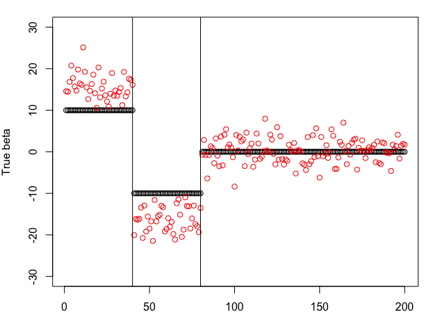
Figure 1: Red points represent MPLE $\hat{\beta_{i}}$, black points represent corresponding true value $\beta_{i0}$

A.6 Proof of Theorem 2

We first present a useful lemma, which is proved in (Huang et al. 2020, Lemma 5.1)

Lemma 6.

For $K>0,a>0$

$$\int_{\|{\boldsymbol{X}}\|_{2}>K}\exp(-a\|{\boldsymbol{X}}\|_{2})d{\boldsymbol{X}}\leq\frac{\Gamma(p)s_{p-1}}{a^{p}}\min\left(1,e^{p-aK}\left(\frac{aK}{p}\right)^{p}\right)$$

where the constant $s_{p-1}=\frac{2\pi^{p/2}}{\Gamma(p/2)}$ is the surface area of $a(p-1)$-dimension sphere. An immediate consequence is that

$$\int\exp(-a\|{\boldsymbol{X}}\|_{2})d{\boldsymbol{X}}=\int_{\|{\boldsymbol{X}}\|_{2}\geq K}\exp(-a\|{\boldsymbol{X}}\|_{2})d{\boldsymbol{X}}+\int_{\|{\boldsymbol{X}}\|_{2}<K}\exp(-a\|{\boldsymbol{X}}\|_{2})d{\boldsymbol{X}}<\infty$$

A.6.1 Properness of catalytic prior with fixed weight

Recall that we have assumed the norm-recoverability condition: $\frac{1}{M}\sum_{i=1}^{M}|{\boldsymbol{X}}_{i}^{*\top}\boldsymbol{\beta}|\geq c_{1}\|\boldsymbol{\beta}\|_{2}$ for all $\boldsymbol{\beta}\in\mathbb{R}^{p}$. Now we are ready to prove that the integral of the catalytic prior is finite.

We first define some constants that are all positive. Let $q=\min_{1\leq i\leq M}Y_{i}^{*}h_{0}^{+}$, $C_{1}:=\prod_{i=1}^{M}[h_{0}^{+}]^{\frac{\tau}{M}}$, $C_{q}:=\max\{0,-2+2\log(\frac{2}{q})\}$. We immediately have

$$\int\pi_{cox,cat}(\boldsymbol{\beta}\mid\tau)d\boldsymbol{\beta}= \int\left[\prod_{i=1}^{M}\left\{\exp\left({\boldsymbol{X}}_{i}^{*\prime}\boldsymbol{\beta}\right)h_{0}^{+}\right\}\exp\left\{-\exp\left({\boldsymbol{X}}_{i}^{*\prime}\boldsymbol{\beta}\right)Y_{i}^{*}h_{0}^{+}\right\}\right]^{\tau/M}d\boldsymbol{\beta}$$ (28)

$$= C_{1}\int\left[\prod_{i=1}^{M}\exp\left\{{\boldsymbol{X}}_{i}^{*\prime}\boldsymbol{\beta}-\exp\left({\boldsymbol{X}}_{i}^{*\prime}\boldsymbol{\beta}\right)Y_{i}^{*}h_{0}^{+}\right\}\right]^{\tau/M}d\boldsymbol{\beta}$$

$$\leq C_{1}\int\exp\left\{\frac{\tau}{M}\sum_{i=1}^{M}\left({\boldsymbol{X}}_{i}^{*\prime}\boldsymbol{\beta}-\exp\left({\boldsymbol{X}}_{i}^{*\prime}\boldsymbol{\beta}\right)q\right)\right\}d\boldsymbol{\beta}$$

$$\leq C_{1}\int\exp\left\{\frac{\tau}{M}\sum_{i=1}^{M}\left(-|{\boldsymbol{X}}_{i}^{*\prime}\boldsymbol{\beta}|+C_{q}\right)\}\right\}d\boldsymbol{\beta}$$

$$= C_{1}\int\exp\left\{\tau C_{q}\right\}\exp\left\{-\frac{\tau}{M}\sum_{i=1}^{M}|{\boldsymbol{X}}_{i}^{*\prime}\boldsymbol{\beta}|\right\}d\boldsymbol{\beta},$$

where the first inequality is due to the definition of the constant $q$, the second inequality follows from the elementary identity that

$$\max_{y}\{y-\alpha e^{y}+|y|\}=\begin{cases}-\alpha,&\text{ if }\alpha\geq 2\\ \max(-\alpha,2\log\frac{2}{\alpha}-2),&\text{ if }\alpha\in(0,2)\end{cases}$$

In view of the norm-recoverability condition, we apply Lemma 6 with $a=\tau c_{1}$ to obtain

$$\text{Righ hand side of \eqref{eq:int-cox-cat} }\leq C_{1}\exp\left\{\tau C_{q}\right\}\int\exp(-\tau c_{1}\|\boldsymbol{\beta}\|_{2})d\boldsymbol{\beta}$$

$$< \infty.$$

A.6.2 Properness of the Cox adaptive catalytic prior

Denote by $\ell(\boldsymbol{\beta})$ the log likelihood based on the synthetic data:

$$\ell(\boldsymbol{\beta})=\frac{1}{M}\sum_{i=1}^{M}\left[\log(h_{0}^{+})+{\boldsymbol{X}}_{i}^{*\prime}\boldsymbol{\beta}-Y_{i}^{*}h_{0}^{+}\exp\left({\boldsymbol{X}}_{i}^{*\prime}\boldsymbol{\beta}\right)\right]$$

and we have $\tau\ell(\boldsymbol{\beta})=\log\pi_{cox,cat}(\boldsymbol{\beta}\mid\tau)$. Based on the proof in previous section, we have

$$\exp(\ell(\boldsymbol{\beta}))\leq C_{1}\exp(C_{q})\exp\left(-c_{1}\|\boldsymbol{\beta}\|\right),\quad\forall\boldsymbol{\beta}\neq 0$$ (29)

Recall $\Gamma_{\alpha,\gamma}(\tau)$ is taken as (10) of the main text, and we have $\kappa\geq\ell(\boldsymbol{\beta})$. By Tonelli’s theorem, for any $\alpha^{\prime}\in(0,\alpha)$,

$$\int_{\tau>0}\int_{\boldsymbol{\beta}\in\mathbb{R}^{p}}\|\boldsymbol{\beta}\|^{\alpha^{\prime}}\tau^{p+\alpha-1}\exp\left(-\left(\kappa+\frac{1}{\gamma}\right)\tau+\tau\ell(\boldsymbol{\beta})\right)d\boldsymbol{\beta}d\tau=\int_{\boldsymbol{\beta}\in\mathbb{R}^{p}}\frac{\|\boldsymbol{\beta}\|^{\alpha^{\prime}}\Gamma(p+\alpha)}{\left(\kappa+\gamma^{-1}-\ell(\boldsymbol{\beta})\right)^{p+\alpha}}d\boldsymbol{\beta}$$

Split the integral above into two: $\int_{\ell(\boldsymbol{\beta})\leq\kappa-c_{1}\|\boldsymbol{\beta}\|/2}$ and $\int_{\ell(\boldsymbol{\beta})>\kappa-c_{1}\|\boldsymbol{\beta}\|/2}$. We will separately bound the two integrals (without the constant term $\Gamma(p+\alpha)$ there). For the first integral, we have

$$\int_{\ell(\boldsymbol{\beta})\leq\kappa-c_{1}\|\boldsymbol{\beta}\|/2}\frac{\|\boldsymbol{\beta}\|^{\alpha^{\prime}}}{(\kappa+1/\gamma-\ell(\boldsymbol{\beta}))^{p+\alpha}}d\boldsymbol{\beta}$$

$$\leq \int_{\ell(\boldsymbol{\beta})\leq\kappa-c_{1}\|\boldsymbol{\beta}\|/2}\frac{\|\boldsymbol{\beta}\|^{\alpha^{\prime}}}{\left(1/\gamma+c_{1}\|\boldsymbol{\beta}\|/2\right)^{p+\alpha}}d\boldsymbol{\beta}\leq\int_{\mathbb{R}^{p}}\frac{\|\boldsymbol{\beta}\|^{\alpha^{\prime}}}{\left(1/\gamma+c_{1}\|\boldsymbol{\beta}\|/2\right)^{p+\alpha}}d\boldsymbol{\beta},$$

where the last integral is finite by elementary calculus.

For the second integral, we have

$$\int_{\ell(\boldsymbol{\beta})>\kappa-c_{1}\|\boldsymbol{\beta}\|/2}\frac{\|\boldsymbol{\beta}\|^{\alpha^{\prime}}}{(\kappa+1/\gamma-\ell(\boldsymbol{\beta}))^{p+\alpha}}d\boldsymbol{\beta}$$

$$\leq \int_{\ell(\boldsymbol{\beta})>\kappa-c_{1}\|\boldsymbol{\beta}\|/2}\frac{\|\boldsymbol{\beta}\|^{\alpha^{\prime}}}{(1/\gamma)^{p+\alpha}}d\boldsymbol{\beta}$$

$$\leq \int_{\ell(\boldsymbol{\beta})>\kappa-c_{1}\|\boldsymbol{\beta}\|/2}\frac{\|\boldsymbol{\beta}\|^{\alpha^{\prime}}}{(1/\gamma)^{p+\alpha}}\exp\left(\ell(\boldsymbol{\beta})+c_{1}\|\boldsymbol{\beta}\|/2-\kappa\right)d\boldsymbol{\beta}$$

$$\leq C_{1}\exp(C_{q})\int_{\ell(\boldsymbol{\beta})>\kappa-c_{1}\|\boldsymbol{\beta}\|/2}\gamma^{p+\alpha}\|\boldsymbol{\beta}\|^{\alpha^{\prime}}e^{-\kappa}\exp\left(-c_{1}\|\boldsymbol{\beta}\|+c_{1}\|\boldsymbol{\beta}\|/2\right)d\boldsymbol{\beta}$$

$$\leq C_{1}\exp(C_{q})\int_{\boldsymbol{\beta}\in\mathbb{R}^{p}}\gamma^{p+\alpha}\|\boldsymbol{\beta}\|^{\alpha^{\prime}}e^{-\kappa}\exp\left(-c_{1}\|\boldsymbol{\beta}\|/2\right)d\boldsymbol{\beta},$$

where the first inequality is because by definition of $\kappa$ it is no less than $\ell(\boldsymbol{\beta})$, the second inequality is due to the fact that $\ell(\boldsymbol{\beta})+c_{1}\|\boldsymbol{\beta}\|/2-\kappa\geq 0$ in the domain of the integral, and the third inequality is due to (29). The last expression is finite due to its exponential tail.

A.7 Proof of Proposition 5

The approach to proving the consistency of $\hat{\boldsymbol{\beta}}_{WM,\tau}$ and $\hat{\boldsymbol{\beta}}_{CR,\tau}$ for given values of $\tau$ and $M$ is straightforward. Since synthetic data become increasingly negligible as the sample size tends to infinity, it is possible to demonstrate that both loss functions converge to the log partial likelihood function as $n$ approaches infinity. The consistency of both estimators can then be established using standard convex theory, since all loss functions are concave. In the subsequent sections, we first present the standard asymptotic theory for MPLE and then establish the proximity of the two estimators to MPLE.

Following the notation and conditions in (Andersen & Gill 1982), define $N_{i}(t)=I\left\{T_{i}\leq t,T_{i}\leq C_{i}\right\}$ and $Y_{i}(t)=I\left\{T_{i}\geq t,C_{i}\geq t\right\}$. We assume that there exists a $T_{0}$ such that $C_{i}\leq T_{0}$ with probability 1 , and that $P\left(Y_{i}(\tau)=1\right)>0$. Thus, $T_{0}$ is the largest possible observed time. Without loss of generality, we take $T_{0}=1$. Following conditions are assume to be true in order to guarantee the consistency of MPLE.

Condition 1

$\int_{0}^{1}h_{0}(t)dt<\infty$

Condition 2

The processes $Y(t)$ is left-continuous with right hand limits, and

$$P\{Y(t)=1\quad\forall t\in[0,1]\}>0$$

Condition 3

There exists a neighborhood $\mathcal{B}$ of $\boldsymbol{\beta}_{0}$ such that

$$E\sup_{t\in[0,1],\boldsymbol{\beta}\in\mathcal{B}}Y(t)\mathbf{x}^{\top}\mathbf{x}\exp\left(\boldsymbol{\beta}^{\top}\mathbf{x}\right\}<\infty.$$

Condition 4

Define

$$s^{(0)}(\boldsymbol{\beta},t)=EY(t)\exp\left\{\boldsymbol{\beta}^{\top}\mathbf{x}\right\},$$

$$s^{(1)}(\boldsymbol{\beta},t)=EY(t)\mathbf{x}\exp\left\{\boldsymbol{\beta}^{\top}\mathbf{x}\right\},$$

$$s^{(2)}(\boldsymbol{\beta},t)=EY(t)\mathbf{x}\mathbf{x}^{\top}\exp\left\{\boldsymbol{\beta}^{\top}\mathbf{x}\right\}$$

where $s^{(0)}(\cdot,t),s^{(1)}(\cdot,t)$ and $s^{(2)}(\cdot,t)$ are continuous in $\boldsymbol{\beta}\in\mathcal{B}$, uniformly in $t\in[0,1].s^{(0)},s^{(1)}$ and $s^{(2)}$ are bounded on $\mathcal{B}\times[0,1];s^{(0)}$ is bounded away from zero on $B\times[0,1]$. Condition 1-4 guarantee the consistency of MPLE.

Condition 5

For all $\boldsymbol{\beta}\in\mathbb{R}^{p}$ with $\tau=o(n)$ , and for all $s\in[0,T_{0}]$

$$\lim_{n\rightarrow\infty}\frac{\tau}{nM}\sum_{j=1}^{M}Y_{j}^{*}(s)e^{\boldsymbol{\beta}^{\prime}{\boldsymbol{X}}_{j}^{*}}=0\quad\text{ in probability}$$

Condition 5 is a technical assumption for proving the consistency of $\hat{\boldsymbol{\beta}}_{WM,\tau}$, which indicates that the influence of synthetic data is dominated by the observed data when we have sufficient observed data.

Next we present a lemma regarding concave function, which is from (Fleming & Harrington 2005, Lemma 8.3.1):

Lemma 7.

Let $E$ be an open convex subset of $\mathbb{R}^{p}$, and let $F_{1},F_{2},\ldots$, be a sequence of random concave functions on $E$ and $f$ a real-valued function on $E$ such that, for all $x\in E$,

$$\lim_{n\rightarrow\infty}F_{n}(x)=f(x)$$

in probability. And if $F_{n}$ has a unique maximum at $X_{n}$ and $f$ has one at $x$, then $X_{n}\rightarrow x$ in probability as $n\rightarrow\infty$.

The key step to show consistency of MPLE is to construct log partial likelihood ratio and show it will converge to its population version. The proof for penalized approach and mix data approach are similar. Define

$$X_{n}(\boldsymbol{\beta},T_{0}) =\frac{1}{n}\left[\log PL(\boldsymbol{\beta})-\log PL(\boldsymbol{\beta}_{0})\right]$$ (30)

$$X_{n,RL}(\boldsymbol{\beta},T_{0}) =\frac{1}{n}\left[\log PL(\boldsymbol{\beta})+\frac{\tau}{M}\log L\left(\boldsymbol{\beta},h_{0}^{+}\mid\left\{\left({\boldsymbol{X}}_{i}^{*},Y_{i}^{*}\right)\right\}_{i=1}^{M}\right)-\right.$$

$$\quad\quad\left.\log PL(\boldsymbol{\beta}_{0})-\frac{\tau}{M}\log L\left(\boldsymbol{\beta}_{0},h_{0}^{+}\mid\left\{\left({\boldsymbol{X}}_{i}^{*},Y_{i}^{*}\right)\right\}_{i=1}^{M}\right)\right]$$

$$X_{n,mix}(\boldsymbol{\beta},T_{0}) =\frac{1}{n}[\log P\tilde{L}(\boldsymbol{\beta})-\log P\tilde{L}(\boldsymbol{\beta}_{0})]$$

It is straightforward to verify that three hessian matrix with respect to $\boldsymbol{\beta}$ is negative definite, which implies that $X_{n}(\boldsymbol{\beta},T_{0}),X_{n,RL}(\boldsymbol{\beta},T_{0}),X_{n,mix}(\boldsymbol{\beta},T_{0})$ are concave function with unique maximizers MPLE, $\hat{\boldsymbol{\beta}}_{CR,\tau}$, $\hat{\boldsymbol{\beta}}_{WM,\tau}$ respectively. The population version is given by

$$A(\boldsymbol{\beta},T_{0})=\int_{0}^{T_{0}}\left[\left(\boldsymbol{\beta}-\boldsymbol{\beta}^{*}\right)^{\prime}s^{(1)}\left(\boldsymbol{\beta}_{0},x\right)-\log\left\{\frac{s^{(0)}(\boldsymbol{\beta},x)}{s^{(0)}\left(\boldsymbol{\beta}_{0},x\right)}\right\}s^{(0)}\left(\boldsymbol{\beta}_{0},x\right)\right]\lambda_{0}(x)dx,$$

Following the proof in (Fleming & Harrington 2005, Theorem 8.3.1), we know $A(\boldsymbol{\beta},T_{0})$ admits unique maximizer $\boldsymbol{\beta}_{0}$ and under condition 1-4:

$$\lim_{n\rightarrow\infty}X_{n}(\boldsymbol{\beta},T_{0})=A(\boldsymbol{\beta},T_{0})\quad\text{ in probability}$$ (31)

Consistency for MPLE is achieved by applying Lemma 7 with $E=\mathbb{R}^{p}$. Therefore, it suffices to show for any $\boldsymbol{\beta}\in\mathbb{R}^{p}$,

$$\lim_{n\rightarrow\infty}X_{n}(\boldsymbol{\beta},T_{0})-X_{n,RL}(\boldsymbol{\beta},T_{0})=0\quad\text{ in probability}$$ (32)

$$\lim_{n\rightarrow\infty}X_{n}(\boldsymbol{\beta},T_{0})-X_{n,mix}(\boldsymbol{\beta},T_{0})=0\quad\text{ in probability}$$ (33)

(32) is easy to establish since penalty term $\frac{\tau}{M}\log L\left(\boldsymbol{\beta},h_{0}^{+}\mid\left\{\left({\boldsymbol{X}}_{i}^{*},Y_{i}^{*}\right)\right\}_{i=1}^{M}\right)=o(n)$ for any $\boldsymbol{\beta}\in\mathbb{R}^{p}$, which further implies that $\hat{\boldsymbol{\beta}}_{CR,\tau}\rightarrow\boldsymbol{\beta}_{0}$ in probability. To show (33), we rewrite $X_{n}(\boldsymbol{\beta},T_{0}),X_{n,mix}(\boldsymbol{\beta},T_{0})$ in the format of integral with respect to counting process.

$$X_{n}(\boldsymbol{\beta},T_{0}) =\frac{1}{n}\left[\log PL(\boldsymbol{\beta})-\log PL(\boldsymbol{\beta}_{0})\right]$$ (34)

$$=n^{-1}\left[\sum_{i=1}^{n}\int_{0}^{T_{0}}\left(\boldsymbol{\beta}-\boldsymbol{\beta}_{0}\right)^{\prime}{\boldsymbol{X}}_{i}-\log\left\{\frac{\frac{1}{n}\sum_{j=1}^{n}Y_{j}(s)e^{\boldsymbol{\beta}^{\prime}{\boldsymbol{X}}_{j}}}{\frac{1}{n}\sum_{j=1}^{n}Y_{j}(s)e^{\boldsymbol{\beta}^{\prime}_{0}{\boldsymbol{X}}_{j}}}\right\}dN_{i}(s)\right]$$

Without loss of generality, we assume first $n$ data in merged dataset are observed data. Otherwise, just reindex to reserve $i=1\ldots n$ for observed data.

$$X_{n,mix}(\boldsymbol{\beta},T_{0}) =\frac{1}{n}[\log P\tilde{L}(\boldsymbol{\beta})-\log P\tilde{L}(\boldsymbol{\beta}^{*})]$$ (35)

$$=\frac{1}{n}\sum_{i=1}^{n}\int_{0}^{T_{0}}\left(\boldsymbol{\beta}-\boldsymbol{\beta}_{0}\right)^{\prime}{\boldsymbol{X}}_{i}-\log\left\{\frac{\frac{1}{n}\sum_{j=1}^{n}Y_{j}(s)e^{\boldsymbol{\beta}^{\prime}{\boldsymbol{X}}_{j}}+\frac{\tau}{nM}\sum_{j=n+1}^{n+M}Y_{j}^{*}(s)e^{\boldsymbol{\beta}^{\prime}{\boldsymbol{X}}_{j}^{*}}}{\frac{1}{n}\sum_{j=1}^{n}Y_{j}(s)e^{\boldsymbol{\beta}^{\prime}_{0}{\boldsymbol{X}}_{j}}+\frac{\tau}{nM}\sum_{j=n+1}^{n+M}Y_{j}^{*}(s)e^{\boldsymbol{\beta}^{\prime}_{0}{\boldsymbol{X}}_{j}^{*}}}\right\}dN_{i}(s)$$

$$+ \frac{\tau}{nM}\sum_{i=n+1}^{n+M}\int_{0}^{T_{0}}\left(\boldsymbol{\beta}-\boldsymbol{\beta}_{0}\right)^{\prime}{\boldsymbol{X}}^{*}_{i}-\log\left\{\frac{\frac{1}{n}\sum_{j=1}^{n}Y_{j}(s)e^{\boldsymbol{\beta}^{\prime}{\boldsymbol{X}}_{j}}+\frac{\tau}{nM}\sum_{j=n+1}^{n+M}Y_{j}^{*}(s)e^{\boldsymbol{\beta}^{\prime}{\boldsymbol{X}}_{j}^{*}}}{\frac{1}{n}\sum_{j=1}^{n}Y_{j}(s)e^{\boldsymbol{\beta}^{\prime}_{0}{\boldsymbol{X}}_{j}}+\frac{\tau}{nM}\sum_{j=n+1}^{n+M}Y_{j}^{*}(s)e^{\boldsymbol{\beta}^{\prime}_{0}{\boldsymbol{X}}_{j}^{*}}}\right\}dN_{i}(s)$$

By law of large number $\frac{1}{n}\sum_{j=1}^{n}Y_{j}(s)e^{\boldsymbol{\beta}^{\prime}_{0}{\boldsymbol{X}}_{j}}\rightarrow s^{(0)}(\boldsymbol{\beta}_{0},s)$ and $\frac{\tau}{nM}\sum_{j=n+1}^{n+M}Y_{j}^{*}(s)e^{\boldsymbol{\beta}^{\prime}{\boldsymbol{X}}_{j}^{*}}=o(1)$ based on condition 5, then for any $\boldsymbol{\beta}\in\mathbb{R}^{p}$, we have

$$\frac{\frac{1}{n}\sum_{j=1}^{n}Y_{j}(s)e^{\boldsymbol{\beta}^{\prime}{\boldsymbol{X}}_{j}}+\frac{\tau}{nM}\sum_{j=n+1}^{n+M}Y_{j}^{*}(s)e^{\boldsymbol{\beta}^{\prime}{\boldsymbol{X}}_{j}^{*}}}{\frac{1}{n}\sum_{j=1}^{n}Y_{j}(s)e^{\boldsymbol{\beta}^{\prime}_{0}{\boldsymbol{X}}_{j}}+\frac{\tau}{nM}\sum_{j=n+1}^{n+M}Y_{j}^{*}(s)e^{\boldsymbol{\beta}^{\prime}_{0}{\boldsymbol{X}}_{j}^{*}}}\rightarrow\frac{s^{(0)}(\boldsymbol{\beta},s)}{s^{(0)}(\boldsymbol{\beta}_{0},s)}\quad\text{ in probability}$$

which implies that for any $\boldsymbol{\beta}\in\mathbb{R}^{p}$,

$$\lim_{n\rightarrow\infty}X_{n}(\boldsymbol{\beta},T_{0})-X_{n,mix}(\boldsymbol{\beta},T_{0})=0\quad\text{ in probability}$$

Apply Lemma 7 and (31), $\hat{\boldsymbol{\beta}}_{WM,\tau}\rightarrow\boldsymbol{\beta}_{0}$ in probability.

We provide a simple simulation to verify the consistency of $\hat{\boldsymbol{\beta}}_{CR,\tau}$ and $\hat{\boldsymbol{\beta}}_{WM,\tau}$ for $p=20,p=50$ and $p=100$. $\boldsymbol{\beta}_{0}\sim$ Unif($\mathbb{S}^{p-1}$)*2, where i.e. $\boldsymbol{\beta}_{0}$ is uniformly distributed on a sphere with length 4. Entries of design matrix $\mathbb{X}$ are generated from standard Gaussian distribution independently. Total number of synthetic data is taken to be $M=400$, synthetic covariate matrix $\mathbb{X}^{*}$ is generated via independent resampling from $\mathbb{X}$. The synthetic response ${\boldsymbol{Y}}^{*}$ is generated in the same manner described in the simulation section. Result is shown in Figure 2.

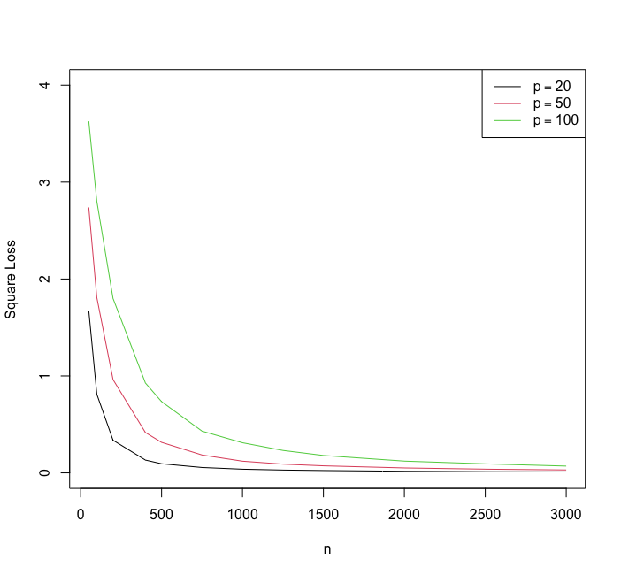
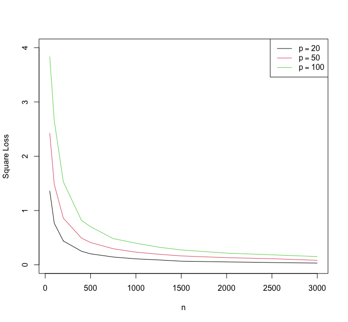
Figure 2: Left hand side: Square Loss $\|\boldsymbol{\beta}_{0}-\hat{\boldsymbol{\beta}}_{CR,p}\|^{2}$ again the sample size for three different dimension. Right hand side: Square Loss $\|\boldsymbol{\beta}_{0}-\hat{\boldsymbol{\beta}}_{WM,p/5}\|^{2}$ again the sample size for three different dimension. It verifies that both approaches provide consistent estimation for true coefficients.

A.8 Implementation of Simulation

The MPLE and the WME in (15) can be computed using standard statistical software; for example, one can use the function coxph($\cdot$) in the R package survival. The CRE in (12) can be obtained using any efficient convex optimization method, such as the classical Newton-Raphson method. Furthermore, we consider Bayesian estimation based on posterior sampling. Specifically, we place a Cox catalytic prior on the coefficients and a Gamma process prior on the cumulative baseline hazard function, collect samples from the posterior distribution, and calculate the posterior mean for the coefficients. For the purpose of comparison, we also consider placing a multivariate Gaussian prior on the coefficients as an alternative.

In addition to the Cox catalytic prior on $\boldsymbol{\beta}$, we also consider the Cox adaptive catalytic prior on $(\boldsymbol{\beta},\tau)$ defined in (9) with hyperparameters $(\alpha,\gamma)$ set to be $(2,1)$. Unlike the other methods, the Cox adaptive catalytic prior has the advantage of being free of tuning parameters.

The Ridge estimator is defined as follows:

$$\hat{\boldsymbol{\beta}}_{\lambda}=\arg\max_{\boldsymbol{\beta}\in\mathbb{R}^{p}}\left\{\sum_{i=1}^{n}\delta_{i}\left({\boldsymbol{X}_{i}}^{\top}\boldsymbol{\beta}-\log\sum_{j\in\mathcal{R}_{i}}\theta_{j}\right)-\lambda f(\boldsymbol{\beta})\right\}$$ (36)

where $\theta_{j}=\exp(\boldsymbol{X}_{j}^{\top}\boldsymbol{\beta})$ and the penalty term $f(\boldsymbol{\beta})=\|\boldsymbol{\beta}\|^{2}$, assuming that each entry of the covariates $\boldsymbol{X}_{i}$’s has been standardized to have zero mean and unit variance. The Lasso estimator is defined in a similar way as in (36) but with $f(\boldsymbol{\beta})=\|\boldsymbol{\beta}\|_{1}$. Both the Ridge and the Lasso estimates can be computed using the glmnet package in R (Simon et al. 2011).

A.9 Selection of tuning parameters

Some of the estimation methods under consideration involve selecting the tuning parameters, including $\tau$ for the estimation based on Cox catalytic prior and $\lambda$ for the penalized estimation using (36). To make a fair comparison, we employed the $K$-fold cross-validation proposed in Van Houwelingen et al. (2006) to select the tuning parameter for each method. To illustrate, we outline the cross-validation procedure for an estimator with tuning parameter $\tau$ and the procedure for $\lambda$ is the same. Given the number $K$ of folds, the original data $\boldsymbol{D}$ is first randomly split into $K$ folds of roughly equal sizes. Then, for each $i$ out of $K$, the $i$-th fold of data is left out and the regression estimate $\widehat{\boldsymbol{\beta}}_{-i}(\tau)$ with tuning parameter $\tau$ is computed based on the remaining $(K-1)$ folds of data. Unlike the standard procedure of cross-validation, where the estimate is used to make prediction on the left-out data, we subtract $\log PL_{-i}\left(\widehat{\boldsymbol{\beta}}_{-i}(\tau)\right)$ from $\log PL\left(\widehat{\boldsymbol{\beta}}_{-i}(\tau)\right)$, where $\log PL$ is the partial log-likelihood for all $K$ folds and $\log PL_{-i}$ is the partial log-likelihood for all folds except the $i$-th. The cross-validated partial log-likelihood is then defined as

$$\text{CVPL}(\tau)=\sum_{i=1}^{K}\left[\log PL\left(\widehat{\boldsymbol{\beta}}_{-i}(\tau)\right)-\log PL_{-i}\left(\widehat{\boldsymbol{\beta}}_{-i}(\tau)\right)\right].$$ (37)

Then the tuning parameter is set to be the value that maximizes the cross-validated partial log-likelihood. For CRE (12) and WME (15), the synthetic data remains the same across different folds.

For CRE, WME, Ridge estimator, Lasso estimator, the tuning parameters are selected by 10-folds cross-validation. For estimation based on Bayesian posterior, the cross-validation requires intensive sampling from different posterior distributions, making it computationally demanding. To reduce the computational burden, a simple approach is to set the total weight parameter equal to the dimension of the regression coefficients, that is, $\tau=p$, as suggested in (Huang et al. 2022) for logistic regression. Another strategy is to utilize the fact that CRE is an approximation to the posterior mode of $\boldsymbol{\beta}$ and can be computed efficiently. Specifically, we first conduct cross-validation to obtain $\hat{\tau}_{CR,cv}$ for CRE and then use its value to specify the hyperparameter $\tau$ for Bayesian posterior estimation. Extending this strategy to Bayesian inference with a normal prior on each coefficient, we first conduct cross-validation to determine $\hat{\lambda}_{2,cv}$ for the Ridge estimator, and set the variance of each normal prior to be $(2\hat{\lambda}_{2,cv})^{-1}$ (assuming that each entry of the observed covariates has been standardized).

A.10 Extra simulation

This section presents additional simulations that extend the numerical study presented in Section 5, in which a censoring rate of 20% was assumed. Specifically, two additional setting is considered, with censoring rates of 10% and 40%.

Table 5: Estimation and prediction performance of the MPLE, Ridge, Lasso, CRE, WME, posterior mean of different Bayesian methods when the censoring rate is 10%. Standard error is presented in parentheses. We indicate the best method for each scenario in bold. Shorthand notations: “CPM", “APM", and “GPM" stand for Bayesian posterior mean resulting from using a Cox catalytic prior, a Cox adaptive catalytic prior, and a Gaussian prior respectively; “CV" in parentheses indicates selection of tuning parameters through cross-validation.

$$\begin{array}[]{clccc}\hline\cr p&\text{Methods}&\|\hat{\boldsymbol{\beta}}-\boldsymbol{\beta}_{0}\|^{2}&\text{ Predictive deviance }\\ \hline\cr\hline\cr&\text{MPLE}&0.84(0.05)&19.35(1.19)\\ &\text{CRE (CV)}&0.57(0.03)&13.25(0.74)\\ &\text{CRE ($\tau=p$)}&0.81(0.02)&19.92(0.72)\\ &\text{WME (CV)}&\textbf{0.48}(0.02)&\textbf{12.83}(0.71)\\ &\text{WME ($\tau=p$)}&1.44(0.02)&38.68(0.84)\\ 20&\text{CPM (CV)}&1.07(0.08)&23.14(0.69)\\ &\text{CPM ($\tau=p$)}&1.01(0.01)&30.12(0.74)\\ &\text{APM}&0.83(0.01)&25.22(0.70)\\ &\text{GPM (CV)}&0.70(0.02)&16.74(0.64)\\ &\text{Ridge (CV)}&0.56(0.03)&13.50(0.65)\\ &\text{Lasso (CV)}&0.71(0.04)&13.99(0.67)\\ \hline\cr\hline\cr&\text{MPLE}&3.39(0.15)&92.77(4.43)\\ &\text{CRE (CV)}&0.77(0.02)&24.66(0.97)\\ &\text{CRE ($\tau=p$)}&0.84(0.01)&26.41(0.83)\\ &\text{WME (CV)}&\textbf{0.74}(0.02)&\textbf{23.88}(0.89)\\ &\text{WME ($\tau=p$)}&1.05(0.01)&32.92(0.81)\\ 40&\text{CPM (CV)}&0.81(0.02)&26.59(0.83)\\ &\text{CPM ($\tau=p$)}&0.92(0.01)&28.72(0.78)\\ &\text{APM}&0.77(0.01)&25.35(0.76)\\ &\text{GPM (CV)}&0.94(0.03)&26.27(0.91)\\ &\text{Ridge (CV)}&0.90(0.03)&25.18(0.95)\\ &\text{Lasso (CV)}&1.18(0.03)&25.50(0.88)\\ \hline\cr\hline\cr&\text{MPLE}&17.60(0.80)&380.56(14.53)\\ &\text{CRE (CV)}&0.98(0.02)&32.38(0.85)\\ &\text{CRE ($\tau=p$)}&0.95(0.01)&31.40(0.77)\\ &\text{WME (CV)}&0.94(0.02)&31.37(0.85)\\ &\text{WME ($\tau=p$)}&1.02(0.01)&33.73(0.71)\\ 60&\text{CPM (CV)}&1.02(0.02)&32.02(0.79)\\ &\text{CPM ($\tau=p$)}&1.01(0.01)&31.50(0.71)\\ &\text{APM}&\textbf{0.91}(0.01)&29.64(0.74)\\ &\text{GPM (CV)}&1.09(0.02)&32.52(0.78)\\ &\text{Ridge (CV)}&1.08(0.02)&32.43(0.79)\\ &\text{Lasso (CV)}&1.29(0.02)&\textbf{29.36}(0.75)\\ \hline\cr\end{array}$$

Table 6: Estimation and prediction performance of the MPLE, Ridge, Lasso, CRE, WME, posterior mean of different Bayesian methods when the censoring rate is 40%. Standard error is presented in parentheses. We indicate the best method for each scenario in bold. See the caption of Table 5 for the meaning of shorthand notations.

$$\begin{array}[]{clccc}\hline\cr p&\text{Methods}&\|\hat{\boldsymbol{\beta}}-\boldsymbol{\beta}_{0}\|^{2}&\text{ Predictive deviance }\\ \hline\cr\hline\cr&\text{MPLE}&1.56(0.11)&23.08(1.50)\\ &\text{CRE (CV)}&0.83(0.05)&13.05(0.81)\\ &\text{CRE ($\tau=p$)}&1.06(0.02)&19.16(0.64)\\ &\text{WME (CV)}&\textbf{0.69}(0.03)&\textbf{12.59}(0.77)\\ &\text{WME ($\tau=p$)}&1.31(0.02)&23.21(0.63)\\ 20&\text{CPM (CV)}&0.76(0.05)&14.08(0.67)\\ &\text{CPM ($\tau=p$)}&1.11(0.02)&20.65(0.62)\\ &\text{APM }&0.74(0.02)&15.08(0.60)\\ &\text{GPM (CV)}&0.73(0.04)&12.97(0.70)\\ &\text{Ridge (CV)}&0.79(0.04)&13.60(0.73)\\ &\text{Lasso (CV)}&1.01(0.04)&13.25(0.66)\\ \hline\cr\hline\cr&\text{MPLE}&10.08(0.67)&148.25(8.46)\\ &\text{CRE (CV)}&1.03(0.03)&22.91(0.78)\\ &\text{CRE ($\tau=p$)}&1.06(0.02)&23.69(0.65)\\ &\text{WME (CV)}&1.00(0.03)&22.51(0.75)\\ &\text{WME ($\tau=p$)}&1.14(0.02)&24.22(0.67)\\ 40&\text{CPM (CV)}&1.05(0.02)&21.78(0.75)\\ &\text{CPM ($\tau=p$)}&1.13(0.02)&23.10(0.68)\\ &\text{APM }&\textbf{0.99}(0.02)&20.62(0.72)\\ &\text{GPM (CV)}&1.10(0.03)&23.67(0.74)\\ &\text{Ridge (CV)}&1.13(0.03)&23.17(0.75)\\ &\text{Lasso (CV)}&1.31(0.03)&\textbf{21.46}(0.73)\\ \hline\cr\hline\cr&\text{MPLE}&683.79(159.72)&1811.07(200.55)\\ &\text{CRE (CV)}&1.16(0.02)&27.05(0.73)\\ &\text{CRE ($\tau=p$)}&\textbf{1.11}(0.01)&26.03(0.74)\\ &\text{WME (CV)}&1.11(0.02)&25.91(0.72)\\ &\text{WME ($\tau=p$)}&1.13(0.01)&25.80(0.74)\\ 60&\text{CPM (CV)}&1.25(0.02)&25.89(0.73)\\ &\text{CPM ($\tau=p$)}&1.22(0.02)&25.13(0.73)\\ &\text{APM }&1.21(0.02)&24.49(0.78)\\ &\text{GPM (CV)}&1.17(0.02)&25.95(0.70)\\ &\text{Ridge (CV)}&1.19(0.02)&26.08(0.73)\\ &\text{Lasso (CV)}&1.34(0.02)&\textbf{22.84}(0.77)\\ \hline\cr\end{array}$$

A.11 Inforamtion about PBC data

The dataset originates from a randomized clinical trial conducted by Mayo Clinic between 1974 and 1984. Its primary objective was to assess the efficacy of a pharmaceutical intervention in the treatment of primary biliary cirrhosis of the liver, which is a rare yet life-threatening disease. The dataset is appealing because it contains a variety of covariates, including both numerical and categorical variables. Researchers have utilized this dataset for building survival models for PBC patients and for investigating the impact of different types of variables (Hoeting et al. 1999).

Our analysis is based on a publicly available version of the dataset, which is included in the R package survival. This dataset includes the following covariates:

• Categorical variables (6 in total): DPCA treatment (2 levels), gender (2 levels), presence of ascites (2 levels), edema (3 levels), hepatomegaly (2 levels), blood vessel malformations in the skin (2 levels);

• Numeric variables (11 in total): age, serum albumin, serum bilirubin, serum cholesterol, alkaline phosphatase, aspartate aminotransferase, urine copper, platelet count, standardized blood clotting time, triglycerides, Histologic stage.

In data preprocessing, we standardized continuous variables and converted categorical variables into binary dummy variables with value 0 or 1. In total, the dimension of a covariate vector is $p=18$ in our analysis. The patient status at the end of the study was coded as 1 for deceased patients and 0 for those still alive. The survival time was defined as the duration in years between the date of registration and the earliest of death, transplantation, or the study’s analysis date in July 1986. After removing subjects with missing data, the PBC dataset consists of $n=276$ observations.

References

- (1)
- Aalen (1989) Aalen, O. O. (1989), ‘A linear regression model for the analysis of life times’, Statistics in medicine 8(8), 907–925.
- Andersen & Gill (1982) Andersen, P. K. & Gill, R. D. (1982), ‘Cox’s regression model for counting processes: a large sample study’, The annals of statistics pp. 1100–1120.
- Beca et al. (2021) Beca, J. M., Chan, K. K., Naimark, D. M. & Pechlivanoglou, P. (2021), ‘Impact of limited sample size and follow-up on single event survival extrapolation for health technology assessment: a simulation study’, BMC Medical Research Methodology 21(1), 1–12.
- Bedrick et al. (1996) Bedrick, E. J., Christensen, R. & Johnson, W. (1996), ‘A new perspective on priors for generalized linear models’, Journal of the American Statistical Association 91(436), 1450–1460.
- Bedrick et al. (1997) Bedrick, E. J., Christensen, R. & Johnson, W. (1997), ‘Bayesian binomial regression: Predicting survival at a trauma center’, The American Statistician 51(3), 211–218.
- Bøvelstad et al. (2007) Bøvelstad, H. M., Nygård, S., Størvold, H. L., Aldrin, M., Borgan, Ø., Frigessi, A. & Lingjærde, O. C. (2007), ‘Predicting survival from microarray data–a comparative study’, Bioinformatics 23(16), 2080–2087.
- Box & Cox (1964) Box, G. E. & Cox, D. R. (1964), ‘An analysis of transformations’, Journal of the Royal Statistical Society: Series B (Methodological) 26(2), 211–243.
- Brard et al. (2017) Brard, C., Le Teuff, G., Le Deley, M.-C. & Hampson, L. V. (2017), ‘Bayesian survival analysis in clinical trials: What methods are used in practice?’, Clinical Trials 14(1), 78–87.
- Bryson & Johnson (1981) Bryson, M. C. & Johnson, M. E. (1981), ‘The incidence of monotone likelihood in the cox model’, Technometrics 23(4), 381–383.
- Chen et al. (2000) Chen, M.-H., Ibrahim, J. G. & Shao, Q.-M. (2000), ‘Power prior distributions for generalized linear models’, Journal of Statistical Planning and Inference 84(1-2), 121–137.
- Chen et al. (2012) Chen, M.-H., Shao, Q.-M. & Ibrahim, J. G. (2012), Monte Carlo methods in Bayesian computation, Springer Series in Statistics, Springer Science & Business Media.
- Cox (1972) Cox, D. R. (1972), ‘Regression models and life-tables’, Journal of the Royal Statistical Society: Series B (Methodological) 34(2), 187–202.
- Cox (1975) Cox, D. R. (1975), ‘Partial likelihood’, Biometrika 62(2), 269–276.
- Fleming & Harrington (2005) Fleming, T. R. & Harrington, D. P. (2005), Counting processes and survival analysis, John Wiley & Sons.
- Gilks & Wild (1992) Gilks, W. R. & Wild, P. (1992), ‘Adaptive rejection sampling for gibbs sampling’, Journal of the Royal Statistical Society: Series C (Applied Statistics) 41(2), 337–348.
- Good (1983) Good, I. J. (1983), Good thinking: The foundations of probability and its applications, U of Minnesota Press.
- Hanson & Jara (2013) Hanson, T. E. & Jara, A. (2013), ‘Surviving fully Bayesian nonparametric regression models’, Bayesian theory and applications pp. 593–615.
- Hoerl & Kennard (1970) Hoerl, A. E. & Kennard, R. W. (1970), ‘Ridge regression: Biased estimation for nonorthogonal problems’, Technometrics 12(1), 55–67.
- Hoeting et al. (1999) Hoeting, J. A., Madigan, D., Raftery, A. E. & Volinsky, C. T. (1999), ‘Bayesian model averaging: a tutorial (with comments by m. clyde, david draper and ei george, and a rejoinder by the authors’, Statistical science 14(4), 382–417.
- Huang et al. (2020) Huang, D., Stein, N., Rubin, D. B. & Kou, S. C. (2020), ‘Catalytic prior distributions with application to generalized linear models’, Proc. Natl. Acad. Sci. U.S.A. 117(22), 12004–12010.
- Huang et al. (2022) Huang, D., Wang, F., Rubin, D. B. & Kou, S. (2022), ‘Catalytic priors: Using synthetic data to specify prior distributions in bayesian analysis’, arXiv preprint arXiv:2208.14123 .
- Huang & Harrington (2002) Huang, J. & Harrington, D. (2002), ‘Penalized partial likelihood regression for right-censored data with bootstrap selection of the penalty parameter’, Biometrics 58(4), 781–791.
- Ibrahim & Chen (1998) Ibrahim, J. G. & Chen, M.-H. (1998), ‘Prior distributions and bayesian computation for proportional hazards models’, Sankhyā: The Indian Journal of Statistics, Series B pp. 48–64.
- Ibrahim & Chen (2000) Ibrahim, J. G. & Chen, M.-H. (2000), ‘Power prior distributions for regression models’, Statistical Science pp. 46–60.
- Ibrahim et al. (2001) Ibrahim, J. G., Chen, M.-H. & Sinha, D. (2001), Bayesian Survival Analysis, Springer Series in Statistics, Springer New York, New York, NY.
- Iwaki (1997) Iwaki, K. (1997), ‘Posterior expected marginal likelihood for testing hypotheses’, J. Econ. Asia Univ 21, 105–134.
- Kalbfleisch (1978) Kalbfleisch, J. D. (1978), ‘Non-parametric bayesian analysis of survival time data’, Journal of the Royal Statistical Society: Series B (Methodological) 40(2), 214–221.
- Kalbfleisch & Prentice (2011) Kalbfleisch, J. D. & Prentice, R. L. (2011), The statistical analysis of failure time data, John Wiley & Sons.
- Latimer (2013) Latimer, N. R. (2013), ‘Survival analysis for economic evaluations alongside clinical trials—extrapolation with patient-level data: inconsistencies, limitations, and a practical guide’, Medical Decision Making 33(6), 743–754.
- Lee et al. (2011) Lee, K. H., Chakraborty, S. & Sun, J. (2011), ‘Bayesian variable selection in semiparametric proportional hazards model for high dimensional survival data’, The International Journal of Biostatistics 7(1), 0000102202155746791301.
- Locke III et al. (1996) Locke III, G. R., Therneau, T. M., Ludwig, J., Dickson, E. R. & Lindor, K. D. (1996), ‘Time course of histological progression in primary biliary cirrhosis’, Hepatology 23(1), 52–56.
- Lovász & Vempala (2006) Lovász, L. & Vempala, S. (2006), Fast algorithms for logconcave functions: Sampling, rounding, integration and optimization, in ‘2006 47th Annual IEEE Symposium on Foundations of Computer Science (FOCS’06)’, IEEE, pp. 57–68.
- Lovász & Vempala (2007) Lovász, L. & Vempala, S. (2007), ‘The geometry of logconcave functions and sampling algorithms’, Random Structures & Algorithms 30(3), 307–358.
- Mills (2010) Mills, M. (2010), ‘Introducing survival and event history analysis’, Introducing Survival and Event History Analysis pp. 1–300.
- Murphy & Van der Vaart (2000) Murphy, S. A. & Van der Vaart, A. W. (2000), ‘On profile likelihood’, Journal of the American Statistical Association 95(450), 449–465.
- Murphy et al. (1997) Murphy, S., Rossini, A. & van der Vaart, A. W. (1997), ‘Maximum likelihood estimation in the proportional odds model’, Journal of the American Statistical Association 92(439), 968–976.
- Neal (2001) Neal, R. (2001), ‘Transferring prior information between models using imaginary data technical report no. 0108’, Department of Statistics, University of Toronto .
- Neuenschwander et al. (2010) Neuenschwander, B., Capkun-Niggli, G., Branson, M. & Spiegelhalter, D. J. (2010), ‘Summarizing historical information on controls in clinical trials’, Clinical Trials 7(1), 5–18.
- Pérez & Berger (2002) Pérez, J. M. & Berger, J. O. (2002), ‘Expected-posterior prior distributions for model selection’, Biometrika 89(3), 491–512.
- Raiffa et al. (1961) Raiffa, H., Schlaifer, R. et al. (1961), ‘Applied statistical decision theory’.
- Saumard & Wellner (2014) Saumard, A. & Wellner, J. A. (2014), ‘Log-concavity and strong log-concavity: a review’, Statistics surveys 8, 45.
- Simon et al. (2011) Simon, N., Friedman, J., Hastie, T. & Tibshirani, R. (2011), ‘Regularization Paths for Cox’s Proportional Hazards Model via Coordinate Descent’, Journal of Statistical Software 39(5), 1–13.
- Sinha (2003) Sinha, D. (2003), ‘A Bayesian justification of Cox’s partial likelihood’, Biometrika 90(3), 629–641.
- Therneau (2023) Therneau, T. M. (2023), A Package for Survival Analysis in R.
- Therneau & Grambsch (2000) Therneau, T. M. & Grambsch, P. M. (2000), Modeling Survival Data: Extending the Cox Model, Statistics for Biology and Health, Springer New York, New York, NY.
- Tibshirani (1997) Tibshirani, R. (1997), ‘The lasso method for variable selection in the cox model’, Statistics in medicine 16(4), 385–395.
- Tsiatis (1981) Tsiatis, A. A. (1981), ‘A large sample study of Cox’s regression model’, The Annals of Statistics 9(1), 93–108.
- Urridge (1981) Urridge, J. (1981), ‘Empirical bayes analysis of survival time data’, Journal of the Royal Statistical Society: Series B (Methodological) 43(1), 65–75.
- Van Houwelingen et al. (2006) Van Houwelingen, H. C., Bruinsma, T., Hart, A. A., Van’t Veer, L. J. & Wessels, L. F. (2006), ‘Cross-validated cox regression on microarray gene expression data’, Statistics in medicine 25(18), 3201–3216.
- van Rosmalen et al. (2018) van Rosmalen, J., Dejardin, D., van Norden, Y., Löwenberg, B. & Lesaffre, E. (2018), ‘Including historical data in the analysis of clinical trials: Is it worth the effort?’, Statistical methods in medical research 27(10), 3167–3182.
- Verweij & Van Houwelingen (1993) Verweij, P. J. & Van Houwelingen, H. C. (1993), ‘Cross-validation in survival analysis’, Statistics in medicine 12(24), 2305–2314.
- Wei (1992) Wei, L.-J. (1992), ‘The accelerated failure time model: a useful alternative to the cox regression model in survival analysis’, Statistics in medicine 11(14-15), 1871–1879.
- Wong (1986) Wong, W. H. (1986), ‘Theory of partial likelihood’, The Annals of statistics pp. 88–123.
- Wu et al. (2018) Wu, J., de Castro, M., Schifano, E. D. & Chen, M.-H. (2018), ‘Assessing covariate effects using jeffreys-type prior in the cox model in the presence of a monotone partial likelihood’, Journal of statistical theory and practice 12, 23–41.
- Zhang et al. (2022) Zhang, X., Zhou, H. & Ye, H. (2022), ‘A modern theory for high-dimensional Cox regression models’, arXiv preprint arXiv:2204.01161 .