The Yukawa-Coupled Dark Sector Model and Cosmological Tensions

Abstract

In this paper, we investigate the interaction between early dark energy (EDE) and cold dark matter, proposing a Yukawa-coupled dark sector model to mitigate cosmological tensions. We utilize the EDE component in the coupled model to relieve the Hubble tension, while leveraging the interaction between dark matter and dark energy to alleviate the large-scale structure tension. The interaction takes the form of Yukawa coupling, which describes the coupling between scalar field and fermion field. We employed various cosmological datasets, including cosmic microwave background radiation, baryon acoustic oscillations, Type Ia supernovae, the local distance-ladder data (SH0ES), and the Dark Energy Survey Year-3 data, to analyze our novel model. Using the Markov Chain Monte Carlo method, our findings reveal that the constrained value of $H_{0}$ obtained from our new model at a 68% confidence level is $72.21^{+0.82}_{-0.69}$ km/s/Mpc, effectively resolving the Hubble tension. Similar to the EDE model, the coupled model yields the $S_{8}$ value that still surpasses the result of the $\Lambda$CDM model. Nevertheless, the best-fit value of $S_{8}$ obtained from our new model is 0.817, which is lower than the EDE model’s result of 0.8316. Consequently, although our model fails to fully resolve the large-scale structure tension, it mitigates the adverse effect of the original EDE model.

I Introduction

As the quantity and precision of cosmological observations continue to improve, the challenges faced by the $\Lambda$CDM model become increasingly severe. Inconsistencies between certain observational results and the predictions of the $\Lambda$CDM model have prompted us to question whether an expansion or replacement of the model is necessary. Prominent examples of these inconsistencies include the Hubble tension and the large-scale structure tension.

The Hubble tension refers to the inconsistency between the value of the Hubble constant, which describes the current rate of cosmic expansion, obtained from local measurements independent of any specific model, and the value inferred from high-redshift cosmic microwave background (CMB) observations based on the $\Lambda$CDM model [1]. Using the distance ladder method, the SH0ES measurement based on Type Ia supernovae yields the value of $H_{0}$ as $73.04\pm 1.04$ km/s/Mpc [2]. However, the Planck 2018 CMB data provides a result of $67.37\pm 0.54$ km/s/Mpc [3], with a statistical error of 4.8$\sigma$.

Another tension frequently mentioned is the conflict between measurements from the CMB and those from observations of large-scale structure [4, 5]. This tension is commonly described by $S_{8}\equiv\sigma_{8}\sqrt{(\Omega_{\mathrm{m}}/0.3)}$, where $\Omega_{m}$ represents the current matter energy density fraction and $\sigma_{8}$ represents the root mean square of matter fluctuations at the scale of 8 $h^{-1}$Mpc. The Planck 2018 best-fit $\Lambda$CDM model gives $S_{8}$ equals to $0.834\pm 0.016$ [3]. However, measurements from the Dark Energy Survey Year-3 (DES-Y3) yield the value of $S_{8}$ as $0.776\pm 0.017$ [6].

In order to address these tensions, a plethora of models have been proposed, including dynamical dark energy model [7, 8, 9], interacting dark energy model [10, 11, 12, 13, 14, 15, 16, 17, 18, 19], early dark energy model [20, 21, 22], axion dark matter model [23, 24], decaying dark matter model [25, 26, 27, 28, 29, 30, 31], and modified gravity model [32, 33, 34, 35], among others.

However, these models generally encounter various challenges and have not fully resolved the cosmological tensions. In this paper, we concentrate on the early dark energy (EDE) model and endeavor to address its related issues.

The EDE model is composed of an extremely light scalar field [36, 37]. In this model, the EDE component reaches its peak at the critical redshift $z_{\mathrm{c}}$, after which its energy density rapidly decays until it becomes negligible. By adjusting the parameters of the EDE model, one can bring $z_{\mathrm{c}}$ closer to the redshift of matter-radiation equality, thereby reducing the comoving sound horizon at the last scattering while maintaining consistency with the angular scale of the sound horizon observed in the CMB, and increasing $H_{0}$. The peak value of the ratio of EDE energy density to total energy density is often represented by $f_{\mathrm{EDE}}$. Generally, resolving the Hubble tension is achievable when $f_{\mathrm{EDE}}$ reaches 10% [21, 38].

However, the EDE model introduces other issues. While the EDE component may be negligible during other periods, it suppresses the growth of structure during its contribution period, thereby impacting other cosmological parameters such as the scalar spectral index $n_{\mathrm{s}}$, matter energy density fluctuations amplitude $\sigma_{8}$, baryon energy density fraction $\omega_{\mathrm{b}}$, and cold dark matter energy density fraction $\omega_{\mathrm{c}}$. As a consequence, the EDE model exacerbates the pre-existing large-scale structure tension [21, 39].

To address this issue, a straightforward approach is to consider the interaction between dark matter and dark energy. The conversion of dark matter into dark energy can reduce the fraction of matter energy density. Additionally, the drag exerted by dark energy on dark matter can suppress clustering effects, thereby mitigating the large-scale structure tension. The interaction between dark matter and dark energy has been extensively studied [40, 41], and can be applied to the EDE model. Alternatively, one can construct the coupling form of the EDE scalar field from fundamental theories [38, 42].

In this study, we employ the Yukawa coupling form, which was originally utilized to describe the interaction between pions and nucleons [43]. Here, we extend its application to characterize the interaction between dark matter and dark energy [44, 45], where the scalar field represents the dark energy component, while the fermion field represents the dark matter component.

We investigated the background and perturbation evolution equations of the Yukawa-coupled dark sector (YCDS) model, and discussed the efficacy of the new model in alleviating the Hubble tension and the large-scale structure tension. We applied the Markov Chain Monte Carlo method to constrain the model parameters using various cosmological data, including the CMB temperature, polarization, and lensing measurements from Planck 2018 [3, 46, 47], baryon acoustic oscillations (BAO) measurements from BOSS DR12 [48, 49], 6dF Galaxy Survey [50], and SDSS DR7 [51], Type Ia supernova sample from Pantheon [52], Hubble constant measurement from SH0ES [2], and $S_{8}$ measurement from Dark Energy Survey Year-3 [6].

The results indicate that the Hubble constant obtained from the coupling model is $72.21^{+0.82}_{-0.69}$ km/s/Mpc at a 68% confidence level, which successfully alleviates the Hubble tension. Similar to the EDE model, the new model exacerbates the large-scale structure tension, and the best-fit value of $S_{8}$ obtained from constraints is 0.817. Nonetheless, compared to the EDE model with the value of 0.8316, the coupling model partially alleviates the negative effect of the original EDE model.

The structure of the paper is as follows. In Sec. II, we derive the evolution equations for the coupling model at both the background and perturbation levels, along with the corresponding initial conditions. Section III presents the numerical results, including the impact on the Hubble parameter and matter power spectrum. In Sec. IV, we present an inventory of the diverse cosmological datasets employed and offer the outcomes of parameter constraint analysis. Finally, in Sec. V, we summarize our research findings.

II Yukawa-coupled dark sector model

The action including early dark energy, cold dark matter, and interaction term takes the following form:

$$\mathcal{S}=\int d^{4}x\sqrt{-g}\left[-\frac{1}{2}\partial^{\mu}\phi\partial_{\mu}\phi-V(\phi)-i\bar{\psi}\not{D}\psi-m_{\psi}\bar{\psi}\psi+\mathcal{L}_{\mathrm{int}}\right].$$ (1)

We represent EDE with a scalar field $\phi$ and adopt the following form for the EDE potential [21, 22]:

$$V(\phi)=m_{\phi}^{2}f_{\phi}^{2}[1-\cos(\phi/f_{\phi})]^{3}+V_{\Lambda},$$ (2)

where $m_{\phi}$ represents the mass of axion, $f_{\phi}$ denotes the axion decay constant, and $V_{\Lambda}$ serves as the cosmological constant. We represent cold dark matter using a fermion field $\psi$, with $m_{\psi}$ denoting its mass. In the non-relativistic limit, $\langle\bar{\psi}\psi\rangle\to n_{\psi}$, $n_{\psi}$ denotes the number density of cold dark matter.

We adopt the Yukawa interaction form to describe the coupling between EDE and cold dark matter,

$$\mathcal{L}_{int}=-\kappa\phi\bar{\psi}\psi,$$ (3)

where $\kappa$ represents the dimensionless Yukawa coupling constant that describes the strength of the interaction. We can absorb the interaction term into the potential term of the fermion field. Specifically, if we use the following transformation form,

$$\kappa=\xi\frac{m_{\psi}}{M_{pl}},$$ (4)

where $\xi$ is a dimensionless constant and $M_{pl}$ represents the reduced Planck mass, then the mass of cold dark matter including the coupling term can be expressed as,

$$m_{c}=m_{\psi}+\kappa\phi=m_{\psi}(1+\frac{\xi\phi}{M_{pl}}).$$ (5)

The energy density of cold dark matter is given by,

$$\rho_{c}=m_{c}n_{\psi}=\widetilde{\rho_{c}}(1+\frac{\xi\phi}{M_{pl}}),$$ (6)

where $\widetilde{\rho_{c}}$ represents the energy density of cold dark matter without interaction. We find that the Yukawa coupling of the dark sector is equivalent to the dependence of the cold dark matter energy density on the EDE scalar. Previous research has utilized the swampland conjecture [53, 54] to propose a coupling form where the dark matter energy density exhibits exponential dependence on the EDE scalar [38, 17]. The Yukawa coupling model can be regarded as a higher-order truncation of the exponential form.

The energy-momentum tensor of cold dark matter is given by,

$$T^{\mu}_{(c)\nu}=m_{c}n_{\psi}u^{\mu}u_{\nu}=\rho_{c}u^{\mu}u_{\nu}$$ (7)

where $u^{\mu}=a^{-1}(1,v^{i})$ represents the four-velocity of cold dark matter and $a$ is the scale factor. We only consider the interaction between dark matter and dark energy, and the sum of their energy-momentum tensors is covariantly conserved,

$$\nabla_{\mu}\left(T^{\mu}_{(\phi)\nu}+T^{\mu}_{(c)\nu}\right)=0.$$ (8)

We separate the energy density of cold dark matter and the EDE scalar into background and perturbation parts for computation,

$$\rho_{c}=\bar{\rho}_{c}+\delta\rho_{c}=\bar{\rho}_{c}(1+\delta_{c}),$$ (9)

$$\phi=\bar{\phi}(\tau)+\delta\phi(\tau,x^{i}),$$ (10)

where $\delta_{c}$ represents the energy density contrast of cold dark matter, and $\tau$ denotes conformal time.

II.1 Background Equations

Expanding the action in Eq.(1) to linear order and carrying out the variation with respect to $\delta\phi$, we obtain the background evolution equation for the EDE scalar,

$$\bar{\phi}^{\prime\prime}+2\mathcal{H}\bar{\phi}^{\prime}+a^{2}V_{\phi}=-a^{2}F\bar{\rho}_{c},$$ (11)

where the prime represents the derivative with respect to conformal time, $\mathcal{H}$ is the conformal Hubble parameter, $V_{\phi}$ denotes the partial derivative of $V(\bar{\phi})$ with respect to the scalar field $\bar{\phi}$, and

$$F=\frac{\xi}{M_{pl}+\xi\bar{\phi}}.$$ (12)

By utilizing the conservation of the total energy-momentum tensor for dark matter and dark energy, in conjunction with Eq.(8) and Eq.(11), we obtain the energy density equation for cold dark matter,

$$\bar{\rho}^{\prime}_{c}+3\mathcal{H}\bar{\rho}_{c}=\bar{\phi}^{\prime}F\bar{\rho}_{c}.$$ (13)

The energy density and pressure of EDE are defined as follows [55],

$$\bar{\rho}_{\phi}=\frac{\bar{\phi}^{\prime 2}}{2a^{2}}+V(\bar{\phi}),$$ (14a)

$$\bar{p}_{\phi}=\frac{\bar{\phi}^{\prime 2}}{2a^{2}}-V(\bar{\phi}).$$ (14b)

Combining the Klein-Gordon equation for the EDE scalar field in Eq.(11), we obtain the energy density evolution equation for EDE,

$$\bar{\rho}_{\phi}^{\prime}+3\mathcal{H}(\bar{\rho}_{\phi}+\bar{p}_{\phi})=-\bar{\phi}^{\prime}F\bar{\rho}_{c}.$$ (15)

In Fig. 1, we illustrate the evolution with redshift of the ratio of EDE energy density to total energy density (left panel) and the EDE scalar (right panel) for different coupling constants. The remaining cosmological parameters are taken from Eq. (20). Different coupling constants lead to variations in the EDE energy density fraction and the amplitude and phase of the EDE scalar. The sign of the coupling constant determines the direction of energy density transfer between dark matter and dark energy. A negative coupling constant results in energy transfer from dark matter to dark energy, leading to a greater EDE energy density fraction, while the effect is reversed for a positive coupling constant.

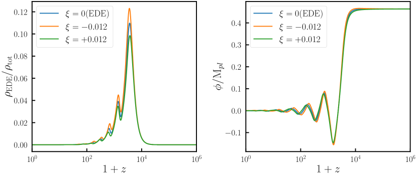
Figure 1: The evolution with redshift of the EDE energy density fraction (left panel) and the EDE scalar (right panel) for various coupling constants is presented. The EDE energy density fraction and the amplitude and phase of the EDE scalar are affected by different coupling constants. Negative coupling constants lead to an increase in the EDE energy density fraction.

II.2 Perturbution equations

We utilize the synchronous gauge to compute the perturbation evolution equations for both EDE and cold dark matter, where the line element is defined as follows,

$$ds^{2}=a^{2}\left[-d\tau^{2}+(\delta_{ij}+h_{ij})dx^{i}dx^{j}\right].$$ (16)

Expanding the action to the quadratic order and taking the variation with respect to $\delta\phi$, we can derive the perturbation evolution equation for the EDE scalar,

$$\delta\phi^{\prime\prime}+2\mathcal{H}\delta\phi^{\prime}+\frac{1}{2}h^{\prime}\bar{\phi}^{\prime}+(k^{2}+a^{2}V_{\phi\phi})\delta\phi=-a^{2}F\bar{\rho}_{c}(\delta_{c}-F\delta\phi),$$ (17)

where $V_{\phi\phi}$ represents the second-order partial derivative of $V(\bar{\phi})$ with respect to $\bar{\phi}$.

By exploiting the covariant conservation of the total energy-momentum tensor for cold dark matter and dark energy, we can derive the evolution equations for the density contrast and velocity divergence of cold dark matter,

$$\delta_{c}^{\prime}+\theta_{c}+\frac{1}{2}h^{\prime}=F(\delta\phi^{\prime}-F\bar{\phi}^{\prime}\delta\phi),$$ (18a)

$$\theta_{c}^{\prime}+\mathcal{H}\theta_{c}=F(k^{2}\delta\phi-\bar{\phi}^{\prime}\theta_{c}).$$ (18b)

II.3 Initial conditions

In the early universe, the dominant influence of Hubble friction in the scalar field causes the scalar field to freeze at its initial value and undergo a slow-roll process. Consequently, the initial value of $\bar{\phi}^{\prime}$ can be set to 0. We consider the ratio of the initial value of $\bar{\phi}$ and the axion decay constant, $\alpha_{i}\equiv\bar{\phi}_{i}/f_{\phi}$ as the model parameter [21, 22].

At this point, the background evolution equation for the energy density of cold dark matter degenerates to the form of the non-coupled case. Hence, we do not alter the initial conditions for cold dark matter. As for the perturbation evolution equations, we adopt adiabatic initial conditions without modifying the initial conditions of the cold dark matter perturbation equations, while the initial conditions for the EDE evolution equations are referenced from [22].

III Numerical results

Based on the description provided in the preceding section, the publicly available Boltzmann code CLASS [56, 57] was modified. We have incorporated a new component of cold dark matter into the calculation of the velocity equation, accounting for the coupling effects. We retain the original component of cold dark matter in CLASS and set $\Omega_{\mathrm{cdm}}=10^{-6}$ to ensure compatibility with the synchronous gauge definition used in the code.

Numerical results are presented using cosmological parameters adopted from Table IV in [38]. The following parameter values are employed for the $\Lambda$CDM model:

$$100\theta{}_{\mathrm{s}}=1.04202,\quad\omega_{\mathrm{b}}=0.02258,$$ (19)

$$\omega_{\mathrm{c}}=0.1176,\quad\ln(10^{10}A_{\mathrm{s}})=3.041,$$

$$n_{\mathrm{s}}=0.9706,\quad\tau_{\mathrm{reio}}=0.0535.$$

For the YCDS model, the value of the coupling constant is exclusively varied, while the values of other cosmological parameters are kept fixed to the constraints obtained from the EDE model,

$$100\theta{}_{\mathrm{s}}=1.04138,\quad\omega_{\mathrm{b}}=0.02281,$$ (20)

$$\omega_{\mathrm{c}}=0.1287,\quad\ln(10^{10}A_{\mathrm{s}})=3.065,$$

$$n_{\mathrm{s}}=0.9895,\quad\tau_{\mathrm{reio}}=0.0581,\quad\alpha_{i}=2.77,$$

$$\log_{10}(f_{\phi})=26.61,\quad\log_{10}(m_{\phi})=-27.31.$$

Figure 2 presents the redshift evolution of the Hubble parameter for different models. The black dotted line represents the $\Lambda$CDM model, while the blue solid line, orange dashed line, and green dash-dotted line correspond to the YCDS model with coupling constants set to 0, $-0.12$, and 0.12, respectively. The 38 datapoints are obtained from [58]. It is noteworthy that when the coupling constant equals 0, the YCDS model degenerates into the EDE model.

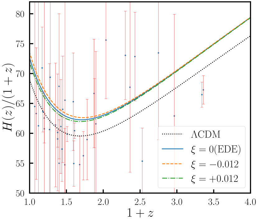
Figure 2: The Hubble parameter evolves with redshift in different models. Different coupling constants impact the magnitude of the Hubble parameter based on the EDE model (with coupling constant $\xi=0$). Negative value of the coupling constant increase the fraction of EDE energy density, thereby indirectly increasing $H_{0}$.

It is evident that the inclusion of the EDE component in the YCDS model leads to a higher Hubble parameter compared to the $\Lambda$CDM model. The magnitude of the Hubble parameter is further influenced by different coupling constants based on the EDE model (with coupling constant $\xi=0$). Negative values of the coupling constant increase the EDE energy density fraction $f_{\mathrm{EDE}}$ (as demonstrated by the influence of different coupling constants on the EDE energy density fraction illustrated in Fig. 1), thereby indirectly leading to an augmentation in the value of $H_{0}$. Conversely, positive value of the coupling constant yield the opposite effect.

We illustrate in Fig. 3 the evolution of $f\sigma_{8}$ with redshift for different models, where 63 Redshift Space Distortion $f\sigma_{8}(z)$ data points are obtained from [59]. The YCDS model yields higher values of $f\sigma_{8}$ than the $\Lambda$CDM model, and different coupling constants affect the results of the original EDE model (with $\xi=0$).

A non-zero coupling constant implies the interaction between dark matter and dark energy, leading to an exchange of energy and momentum between them. Specifically, a negative value of the coupling constant corresponds to the transfer of energy density from dark matter to dark energy, which suppresses the growth of matter structure and reduces $f\sigma_{8}$.

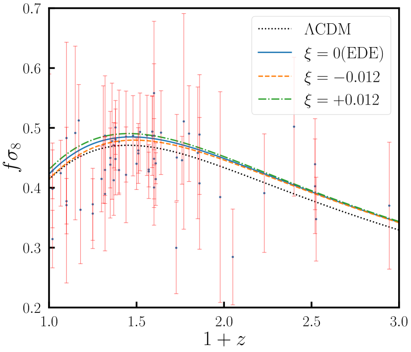
Figure 3: The evolution of $f\sigma_{8}$ with redshift varies across different models. The presence of the EDE component in the YCDS model results in higher $f\sigma_{8}$ values compared to the $\Lambda$CDM model. Different coupling constants modify the outcomes of the original EDE model, with negative value of the coupling constant leading to a reduction in $f\sigma_{8}$.

In Fig. 4, we showcase the linear matter power spectrum (upper panel) and the difference in power spectrum relative to the $\Lambda$CDM model (lower panel) for various models. Consistent with our previous discussion, the interaction between dark matter and dark energy affects the growth of matter structures and alters the shape of the power spectrum.

Negative value of the coupling constant correspond to the transfer of energy density from dark matter to dark energy, reducing the amount of dark matter, together with the drag effect of dark energy on dark matter, this suppresses the clustering of matter and results in smaller $P(k)$ spectra on small scales compared to the original EDE model.

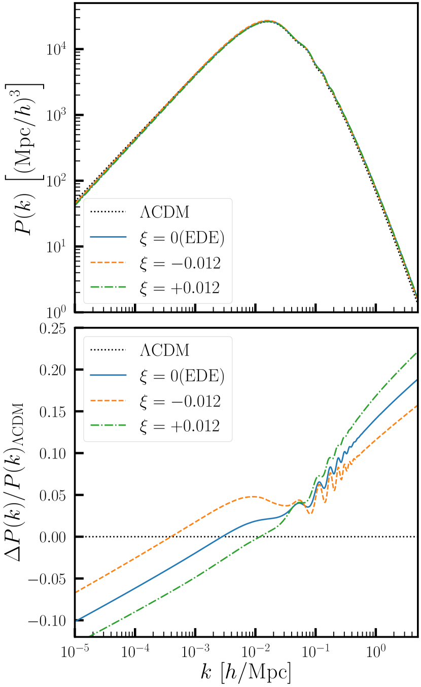
Figure 4: The linear matter power spectra (upper panel) and the differences in power spectra relative to the $\Lambda$CDM model (lower panel) are presented for different models. Negative values of the coupling constant exhibit a reduction in the matter power spectrum on small scales, while positive values of the coupling constant have the opposite effect.

IV Data and Methodology

We utilized MontePython [60, 61] to execute the Markov Chain Monte Carlo (MCMC) analysis to obtain the posterior distribution of model parameters. Subsequently, we employed GetDist [62] to analyze the MCMC chains.

IV.1 Datasets

We employed the following cosmological data to perform the MCMC analysis:

• CMB: The temperature and polarization power spectra measured of both the low-$\ell$ and high-$\ell$ from the Planck 2018 data, as well as the CMB lensing power spectrum. [46, 47, 3].

• BAO: The measurements from the BOSS-DR12 $f\sigma_{8}$ sample, which included the LOWZ and CMASS galaxy samples [48, 49], as well as low-redshift measurements from the 6dFGS and the SDSS DR7 surveys [50, 51].

• Supernovae: The Pantheon sample, consisting of 1048 Type Ia supernova data, covered a redshift range from 0.01 to 2.3 [52].

By combining CMB and BAO data, it becomes possible to perform multiple acoustic horizon measurements at different redshifts. This approach effectively mitigates geometric degeneracies and constrains physical processes between recombination and the BAO measurement redshift. Additionally, the inclusion of supernova data from the Pantheon sample significantly restricts new physics that may be specific to the late epoch within the measured redshift range.

• SH0ES: According to the most recent SH0ES measurement, the value of the Hubble constant has been estimated as $73.04\pm 1.04$ km/s/Mpc [2].

• DES-Y3: The Dark Energy Survey Year-3 incorporates weak lensing and galaxy cluster data, with a Gaussian constraint on the parameter $S_{8}$ of $0.776\pm 0.017$ [6].

We incorporate the $H_{0}$ measurement obtained from SH0ES to address the prior volume effect [63] and assess the efficacy of our novel model in resolving the tension between the local measurement of $H_{0}$ and the results derived from CMB analysis. Additionally, we include the $S_{8}$ data from DES-Y3 to investigate the model’s ability to alleviate the large-scale structure tension.

IV.2 Results

The parameter constraint results for the $\Lambda$CDM model, EDE model, and YCDS model are presented in Tab. 1, where we utilized the complete dataset including CMB, BAO, SNIa, SH0ES, and $S_{8}$ measurement from DES-Y3. The upper section of the table displays the parameters used for MCMC sampling, while the lower section presents the derived parameters.

Table 1: The best-fit values and 68% confidence level parameter constraints are presented for the $\Lambda$CDM, EDE, and YCDS models, utilizing the dataset including CMB, BAO, SNIa, SH0ES, and $S_{8}$ measurement from DES-Y3. The upper section of the table displays the parameters utilized for MCMC sampling, while the lower section shows the derived parameters.

Model	$\Lambda$CDM	EDE	YCDS
$100\omega{}_{\mathrm{b}}$	$2.260(2.263\pm 0.014)$	$2.276(2.281^{+0.024}_{-0.020})$	$2.257(2.274^{+0.020}_{-0.023})$
$\omega{}_{\mathrm{c}}$	$0.11729(0.11725\pm 0.00084)$	$0.1310(0.1299\pm 0.0028)$	$0.1293(0.1292\pm 0.0026)$
$H_{0}$	$68.64(68.71^{+0.35}_{-0.41})$	$71.85(72.46\pm 0.86)$	$71.79(72.21^{+0.82}_{-0.69})$
$\ln(10^{10}A_{\mathrm{s}})$	$3.047(3.050\pm 0.015)$	$3.057(3.063^{+0.015}_{-0.017})$	$3.048(3.061\pm 0.015)$
$n_{\mathrm{s}}$	$0.9733(0.9722\pm 0.0040)$	$0.9877(0.9908\pm 0.0059)$	$0.9838(0.9884\pm 0.0057)$
$\tau{}_{\mathrm{reio}}$	$0.0576(0.0592\pm 0.0082)$	$0.0539(0.0563\pm 0.0090)$	$0.0517(0.0564^{+0.0068}_{-0.0086})$
$\log_{10}(m_{\phi})$	$-$	$-27.292(-27.290\pm 0.055)$	$-27.340(-27.308^{+0.055}_{-0.067})$
$\log_{10}(f_{\phi})$	$-$	$26.632(26.616^{+0.056}_{-0.033})$	$26.609(26.618\pm 0.049)$
$\alpha_{\mathrm{i}}$	$-$	$2.762(2.783\pm 0.069)$	$2.697(2.727^{+0.061}_{-0.054})$
$\xi$	$-$	$-$	$-0.023(-0.011^{+0.013}_{-0.015})$
$10^{-9}A_{\mathrm{s}}$	$2.105(2.112\pm 0.032)$	$2.127(2.139^{+0.031}_{-0.036})$	$2.108(2.135\pm 0.032)$
$100\theta{}_{\mathrm{s}}$	$1.04206(1.04217^{+0.00025}_{-0.00031})$	$1.04121(1.04145\pm 0.00043)$	$1.04141(1.04145\pm 0.00037)$
$f_{\mathrm{EDE}}$	$-$	$0.1183(0.119^{+0.023}_{-0.018})$	$0.1146(0.116^{+0.022}_{-0.018})$
$\log_{10}(z_{\mathrm{c}})$	$-$	$3.571(3.568\pm 0.034)$	$3.540(3.560^{+0.034}_{-0.039})$
$\Omega{}_{\mathrm{m}}$	$0.2983(0.2977\pm 0.0048)$	$0.2991(0.2923\pm 0.0056)$	$0.2959(0.2927^{+0.0050}_{-0.0041})$
$\sigma_{8}$	$0.8039(0.8047\pm 0.0060)$	$0.8329(0.8325\pm 0.0083)$	$0.8227(0.8294\pm 0.0077)$
$S_{8}$	$0.8016(0.8016^{+0.0096}_{-0.0080})$	$0.8316(0.822^{+0.011}_{-0.0093})$	$0.8170(0.819\pm 0.010)$
$\Delta\chi^{2}_{\mathrm{tot}}$	$-$	$-11.74$	$-17.92$
$\Delta\mathrm{AIC}$	$-$	$-5.74$	$-9.92$

Note that the best-fit value of the constrained coupling constant $\xi$ is $-0.023$, and with a 68% confidence level result of $-0.011^{+0.013}_{-0.015}$. This suggests an interaction between dark matter and dark energy, specifically the transfer of energy from dark matter to dark energy, consistent with the expectations discussed in Sec. III.

The constrained value of $H_{0}$ for the YCDS model closely approximate that of the EDE model, being $72.21^{+0.82}_{-0.69}$ km/s/Mpc and $72.46\pm 0.86$ km/s/Mpc, respectively, at a 68% confidence level, both exceeding the value of $68.71^{+0.35}_{-0.41}$ km/s/Mpc for the $\Lambda$CDM model. This indicates that our coupling model inherits the ability of the EDE model to alleviate the Hubble tension.

Similar to the EDE model, the YCDS model yields a larger value of $S_{8}$, with a best-fit value of 0.817, surpassing the value of 0.8016 for the $\Lambda$CDM model. However, compared to the $S_{8}$ value of 0.8316 for the EDE model, the YCDS model mitigates the negative effect of the EDE model and partially alleviates the large-scale structure tension caused by the EDE component.

The impact of the coupling model on the parameters $H_{0}$ and $S_{8}$ can be more easily observed from the posterior distribution plots of selected parameters for the three models in Fig. 5. The complete posterior distributions are presented in Fig. 6 of the appendix section.

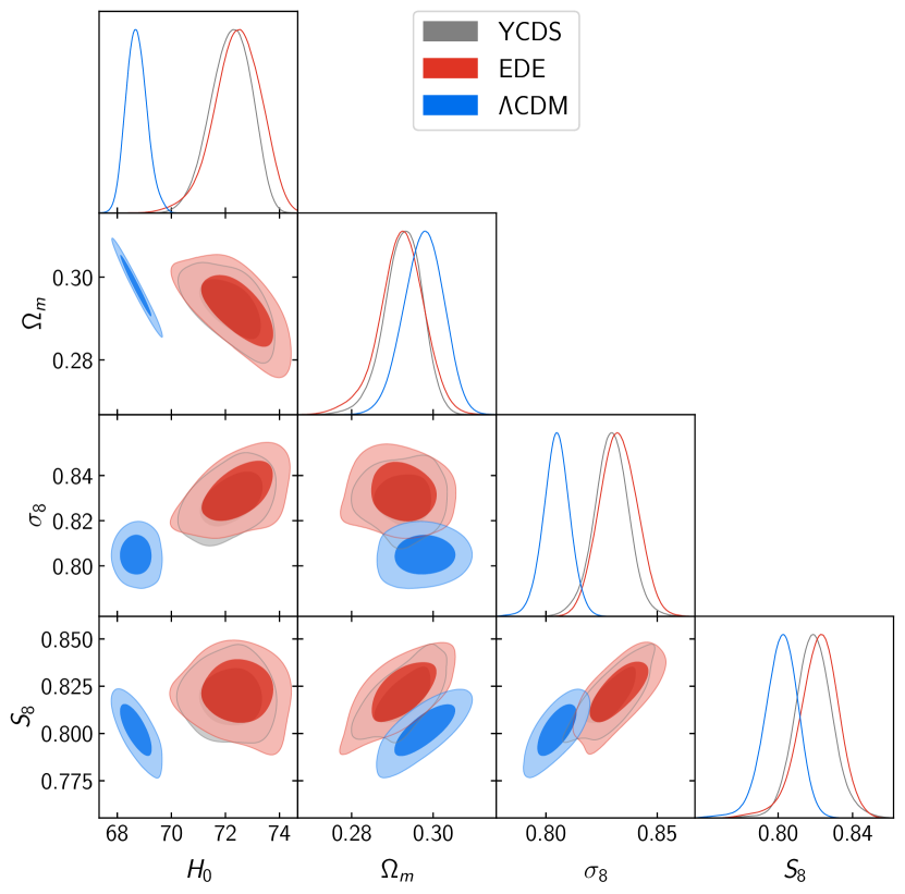
Figure 5: The posterior distributions of selected parameters for the three models are examined. Compared to the $\Lambda$CDM model, both the YCDS and EDE models exhibit larger values of $H_{0}$ and $S_{8}$. In the YCDS model, the interaction between dark matter and dark energy suppresses structure growth, resulting in a reduction in the value of $S_{8}$ compared to the EDE model.

The interaction between dark matter and dark energy in the coupling model inhibits structure growth, thereby reducing the clustering effects of matter. Consequently, the YCDS model results in a smaller value of $S_{8}$ compared to the EDE model.

The penultimate row of Tab. 1 displays the differences in the $\chi^{2}_{\mathrm{tot}}$ values relative to the $\Lambda$CDM model for the EDE and YCDS models, which are $-11.74$ and $-17.92$, respectively. Both models yield a lower $\chi^{2}_{\mathrm{tot}}$ value compared to the $\Lambda$CDM model, primarily driven by the SH0ES data. Additionally, we observe that the YCDS model yields a smaller $\chi^{2}_{\mathrm{tot}}$ value than the EDE model, attributed to the smaller $S_{8}$ constraint obtained by the YCDS model, which aligns more closely with the result obtained from the DES-Y3 data.

In order to compare the models, we computed the the Akaike information criterion (AIC) [64],

$$\mathrm{AIC}=\chi^{2}_{\mathrm{tot}}+2k,$$ (21)

where $k$ represents the number of fitted parameters. The AIC values for the EDE model and the YCDS model relative to the $\Lambda$CDM model are presented in the last row of Tab. 1, as $-5.74$ and $-9.92$, respectively. It is evident that the AIC value for the YCDS model is the smallest, indicating that, from the perspective of AIC, the coupled model performs the best.

V Conclusions

In this paper, we explore the interaction between early dark energy (EDE) and cold dark matter, and propose the Yukawa-coupled dark sector (YCDS) model to alleviate cosmological tensions. We utilize the EDE component within the coupled model to mitigate the Hubble tension, and leverage the interaction between dark matter and dark energy to alleviate the large-scale structure tension. We adopt the Yukawa coupling form that describes the interaction between scalar and fermion fields, and through transformation, this coupling translates into a form where the dark matter energy density depends on the EDE scalar.

We investigate the background and perturbation evolution equations of the coupled model and provide corresponding initial conditions. We discuss the impact of the interaction between dark matter and dark energy on the EDE energy density fraction, Hubble parameter, and structure growth. By employing the MCMC method and utilizing various cosmological datasets including CMB, BAO, SNIa, SH0ES, and $S_{8}$ measurement from DES-Y3, we constrain the parameters of the new model.

We constrained the best-fit value of the coupling constant to be $-0.023$. The negative value of the coupling constant indicates an interaction between dark matter and dark energy, with energy flowing from dark matter to dark energy. In addition, the drag effect of dark energy on dark matter inhibits structure growth, thereby contributing to the alleviation of the large-scale structure tension.

The YCDS model constrains the value of $H_{0}$ to be $72.21^{+0.82}_{-0.69}$ km/s/Mpc at a 68% confidence level, which is greater than the value $68.71^{+0.35}_{-0.41}$ km/s/Mpc in the $\Lambda$CDM model, thereby alleviating the Hubble tension. The best-fit values of $S_{8}$ obtained from the EDE and YCDS models are 0.8316 and 0.817, respectively, both exceeding the value 0.8016 in the $\Lambda$CDM model. However, the interaction between dark matter and dark energy in the new model suppresses the clustering of matter, resulting in a lower $S_{8}$ value than that of the EDE model. Therefore, while the YCDS model does not completely resolve the large-scale structure tension, it mitigates the negative effect of the original EDE model.

We computed the $\chi^{2}_{\mathrm{tot}}$ values of the EDE model and the YCDS model relative to the $\Lambda$CDM model, resulting in values of $-11.74$ and $-17.92$, respectively. To compare the models, we calculated the Akaike information criterion (AIC), which yielded results of $-5.74$ and $-9.92$ for the EDE model and the YCDS model relative to the $\Lambda$CDM model. The coupled model has the lowest AIC value, indicating that from the AIC perspective, our new model performs the best.

The YCDS model, built upon the EDE framework, offers a mitigation of the Hubble tension. While the coupled model fails to fully resolve the large-scale structure tension, it yields the $S_{8}$ value smaller than that obtained from the EDE model, thereby alleviating the negative effect associated with the original EDE model. Further efforts are still required to completely address the cosmological tensions.

*

Appendix A The complete MCMC posterior distributions

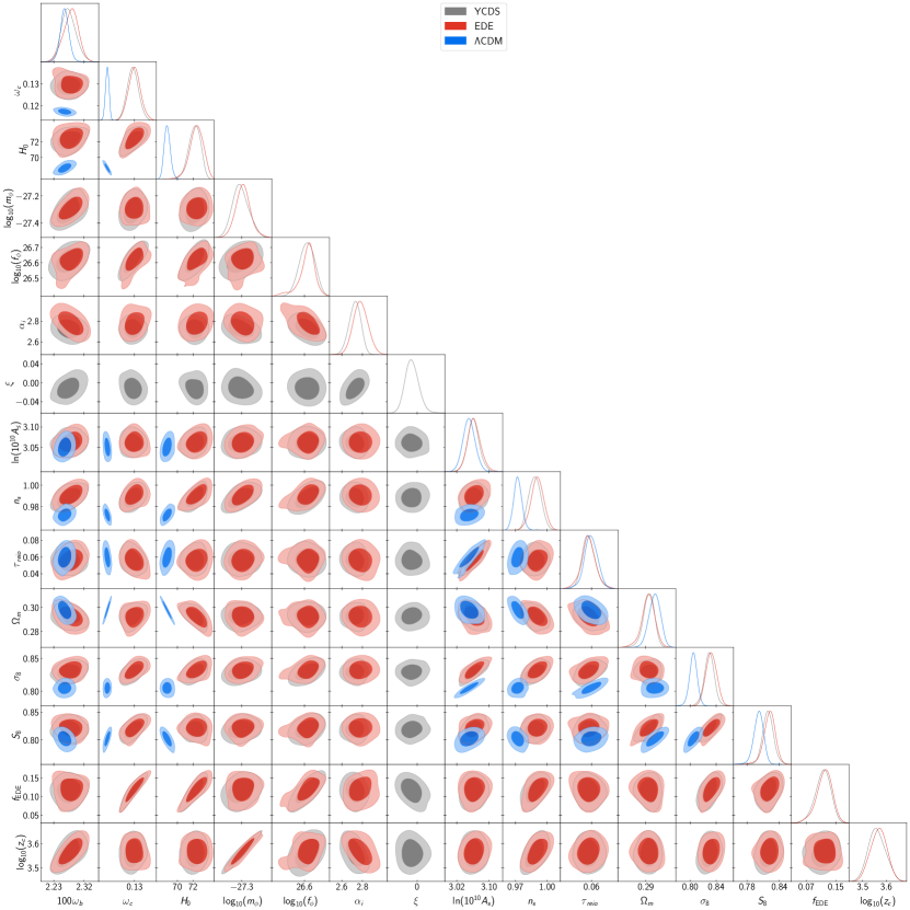
Figure 6: The posterior distribution of the complete parameters for the YCDS model, EDE model, and $\Lambda$CDM model. We utilized all data, including CMB, BAO, SNIa, SH0ES, and $S_{8}$ measurement from DES-Y3.

References

- Verde et al. [2019] L. Verde, T. Treu, and A. G. Riess, Tensions between the early and late universe, Nature Astronomy 3, 891 (2019).
- Riess et al. [2022] A. G. Riess, W. Yuan, L. M. Macri, et al., A comprehensive measurement of the local value of the hubble constant with 1 km/s/mpc uncertainty from the hubble space telescope and the sh0es team, The Astrophysical Journal Letters 934, L7 (2022).
- Planck Collaboration et al. [2020] Planck Collaboration, Aghanim, N., Akrami, Y., et al., Planck 2018 results - VI. Cosmological parameters, Astronomy and Astrophysics 641, A6 (2020).
- Macaulay et al. [2013] E. Macaulay, I. K. Wehus, and H. K. Eriksen, Lower growth rate from recent redshift space distortion measurements than expected from planck, Phys. Rev. Lett. 111, 161301 (2013).
- Hildebrandt et al. [2020] H. Hildebrandt, F. Köhlinger, J. Busch, et al., Kids+viking-450: Cosmic shear tomography with optical and infrared data, Astronomy & Astrophysics 633, A69 (2020).
- Abbott et al. [2022] T. M. C. Abbott, M. Aguena, A. Alarcon, et al., Dark energy survey year 3 results: Cosmological constraints from galaxy clustering and weak lensing, Phys. Rev. D 105, 023520 (2022).
- Guo et al. [2019] R.-Y. Guo, J.-F. Zhang, and X. Zhang, Can the tension be resolved in extensions to lcdm cosmology?, Journal of Cosmology and Astroparticle Physics 2019 (02), 054.
- Li and Shafieloo [2019] X. Li and A. Shafieloo, A simple phenomenological emergent dark energy model can resolve the hubble tension, The Astrophysical Journal Letters 883, L3 (2019).
- Zhou et al. [2022] Z. Zhou, G. Liu, Y. Mu, and L. Xu, Can phantom transition at 1 restore the Cosmic concordance?, Monthly Notices of the Royal Astronomical Society 511, 595 (2022).
- Wang et al. [2016] B. Wang, E. Abdalla, F. Atrio-Barandela, and D. Pavón, Dark matter and dark energy interactions: theoretical challenges, cosmological implications and observational signatures, Reports on Progress in Physics 79, 096901 (2016).
- Koyama et al. [2009] K. Koyama, R. Maartens, and Y.-S. Song, Velocities as a probe of dark sector interactions, Journal of Cosmology and Astroparticle Physics 2009 (10), 017.
- Yang et al. [2017] W. Yang, S. Pan, and D. F. Mota, Novel approach toward the large-scale stable interacting dark-energy models and their astronomical bounds, Phys. Rev. D 96, 123508 (2017).
- Mukherjee and Banerjee [2016] A. Mukherjee and N. Banerjee, In search of the dark matter dark energy interaction: a kinematic approach, Classical and Quantum Gravity 34 (2016).
- Olivares et al. [2008] G. Olivares, F. Atrio-Barandela, and D. Pavón, Dynamics of interacting quintessence models: Observational constraints, Phys. Rev. D 77, 063513 (2008).
- Yang et al. [2018] W. Yang, S. Pan, L. Xu, and D. F. Mota, Effects of anisotropic stress in interacting dark matter-dark energy scenarios, Monthly Notices of the Royal Astronomical Society 482, 1858 (2018).
- Valentino et al. [2020] E. D. Valentino, A. Melchiorri, O. Mena, and S. Vagnozzi, Interacting dark energy in the early 2020s: A promising solution to the and cosmic shear tensions, Physics of the Dark Universe 30, 100666 (2020).
- Liu et al. [2023a] G. Liu, Z. Zhou, Y. Mu, and L. Xu, Alleviating cosmological tensions with a coupled scalar fields model, Phys. Rev. D 108, 083523 (2023a).
- Liu et al. [2023b] G. Liu, Z. Zhou, Y. Mu, and L. Xu, Kinetically coupled scalar fields model and cosmological tensions (2023b), arXiv:2308.07069 [astro-ph.CO] .
- Liu et al. [2023c] G. Liu, J. Gao, Y. Han, Y. Mu, and L. Xu, Mitigating cosmological tensions via momentum-coupled dark sector model (2023c), arXiv:2310.09798 [astro-ph.CO] .
- Poulin et al. [2019] V. Poulin, T. L. Smith, T. Karwal, and M. Kamionkowski, Early dark energy can resolve the hubble tension, Phys. Rev. Lett. 122, 221301 (2019).
- Hill et al. [2020] J. C. Hill, E. McDonough, M. W. Toomey, and S. Alexander, Early dark energy does not restore cosmological concordance, Phys. Rev. D 102, 043507 (2020).
- Smith et al. [2020] T. L. Smith, V. Poulin, and M. A. Amin, Oscillating scalar fields and the hubble tension: A resolution with novel signatures, Phys. Rev. D 101, 063523 (2020).
- D’Eramo et al. [2018] F. D’Eramo, R. Z. Ferreira, A. Notari, and J. L. Bernal, Hot axions and the tension, Journal of Cosmology and Astroparticle Physics 2018 (11), 014.
- Liu et al. [2023d] G. Liu, Y. Mu, Z. Zhou, and L. Xu, Cosmological constraints on thermal friction of axion dark matter (2023d), arXiv:2309.02170 [astro-ph.CO] .
- Vattis et al. [2019] K. Vattis, S. M. Koushiappas, and A. Loeb, Dark matter decaying in the late universe can relieve the tension, Phys. Rev. D 99, 121302 (2019).
- Buch et al. [2017] J. Buch, P. Ralegankar, and V. Rentala, Late decaying 2-component dark matter scenario as an explanation of the ams-02 positron excess, Journal of Cosmology and Astroparticle Physics 2017 (10), 028.
- Bringmann et al. [2018] T. Bringmann, F. Kahlhoefer, K. Schmidt-Hoberg, and P. Walia, Converting nonrelativistic dark matter to radiation, Phys. Rev. D 98, 023543 (2018).
- Clark et al. [2021] S. J. Clark, K. Vattis, and S. M. Koushiappas, Cosmological constraints on late-universe decaying dark matter as a solution to the tension, Phys. Rev. D 103, 043014 (2021).
- Pandey et al. [2020] K. L. Pandey, T. Karwal, and S. Das, Alleviating the and anomalies with a decaying dark matter model, Journal of Cosmology and Astroparticle Physics 2020 (07), 026.
- Alvi et al. [2022] S. Alvi, T. Brinckmann, M. Gerbino, M. Lattanzi, and L. Pagano, Do you smell something decaying? updated linear constraints on decaying dark matter scenarios, Journal of Cosmology and Astroparticle Physics 2022 (11), 015.
- McCarthy and Hill [2023] F. McCarthy and J. C. Hill, Converting dark matter to dark radiation does not solve cosmological tensions, Phys. Rev. D 108, 063501 (2023).
- El-Zant et al. [2019] A. El-Zant, W. E. Hanafy, and S. Elgammal, tension and the phantom regime: A case study in terms of an infrared f(t) gravity, The Astrophysical Journal 871, 210 (2019).
- Khosravi et al. [2019] N. Khosravi, S. Baghram, N. Afshordi, and N. Altamirano, tension as a hint for a transition in gravitational theory, Phys. Rev. D 99, 103526 (2019).
- Renk et al. [2017] J. Renk, M. Zumalacárregui, F. Montanari, and A. Barreira, Galileon gravity in light of isw, cmb, bao and data, Journal of Cosmology and Astroparticle Physics 2017 (10), 020.
- Braglia et al. [2020] M. Braglia, M. Ballardini, W. T. Emond, F. Finelli, A. E. Gümrükçüoğlu, K. Koyama, and D. Paoletti, Larger value for by an evolving gravitational constant, Phys. Rev. D 102, 023529 (2020).
- Kamionkowski et al. [2014] M. Kamionkowski, J. Pradler, and D. G. E. Walker, Dark energy from the string axiverse, Phys. Rev. Lett. 113, 251302 (2014).
- Marsh [2016] D. J. Marsh, Axion cosmology, Physics Reports 643, 1 (2016), axion cosmology.
- McDonough et al. [2022] E. McDonough, M.-X. Lin, J. C. Hill, W. Hu, and S. Zhou, Early dark sector, the hubble tension, and the swampland, Phys. Rev. D 106, 043525 (2022).
- D’Amico et al. [2021] G. D’Amico, L. Senatore, P. Zhang, and H. Zheng, The hubble tension in light of the full-shape analysis of large-scale structure data, Journal of Cosmology and Astroparticle Physics 2021 (05), 072.
- Bertolami et al. [2012] O. Bertolami, P. Carrilho, and J. Páramos, Two-scalar-field model for the interaction of dark energy and dark matter, Phys. Rev. D 86, 103522 (2012).
- Alexander et al. [2023] S. Alexander, H. Bernardo, and M. W. Toomey, Addressing the hubble and tensions with a kinetically mixed dark sector, Journal of Cosmology and Astroparticle Physics 2023 (03), 037.
- Lin et al. [2023] M.-X. Lin, E. McDonough, J. C. Hill, and W. Hu, Dark matter trigger for early dark energy coincidence, Phys. Rev. D 107, 103523 (2023).
- Yukawa [1955] H. Yukawa, On the Interaction of Elementary Particles. I, Progress of Theoretical Physics Supplement 1, 1 (1955).
- Farrar and Peebles [2004] G. R. Farrar and P. J. E. Peebles, Interacting dark matter and dark energy, The Astrophysical Journal 604, 1 (2004).
- Archidiacono et al. [2022] M. Archidiacono, E. Castorina, D. Redigolo, and E. Salvioni, Unveiling dark fifth forces with linear cosmology, Journal of Cosmology and Astroparticle Physics 2022 (10), 074.
- Aghanim et al. [2020a] N. Aghanim, Y. Akrami, M. Ashdown, et al., Planck 2018 results. v. cmb power spectra and likelihoods, Astronomy and Astrophysics 641, 10.1051/0004-6361/201936386 (2020a).
- Aghanim et al. [2020b] N. Aghanim, Y. Akrami, M. Ashdown, et al., Planck 2018 results - viii. gravitational lensing, Astronomy and Astrophysics 641, 10.1051/0004-6361/201833886 (2020b).
- Alam et al. [2017] S. Alam, M. Ata, S. Bailey, et al., The clustering of galaxies in the completed SDSS-III baryon oscillation spectroscopic survey: cosmological analysis of the DR12 galaxy sample, Monthly Notices of the Royal Astronomical Society 470, 2617 (2017).
- Buen-Abad et al. [2018] M. A. Buen-Abad, M. Schmaltz, J. Lesgourgues, and T. Brinckmann, Interacting dark sector and precision cosmology, Journal of Cosmology and Astroparticle Physics 2018 (01), 008.
- Beutler et al. [2011] F. Beutler, C. Blake, M. Colless, et al., The 6df galaxy survey: baryon acoustic oscillations and the local hubble constant, Monthly Notices of the Royal Astronomical Society 416, 3017 (2011).
- Ross et al. [2015] A. J. Ross, L. Samushia, C. Howlett, et al., The clustering of the sdss dr7 main galaxy sample-i. a 4 percent distance measure at , Monthly Notices of the Royal Astronomical Society 449, 835 (2015).
- Scolnic et al. [2018] D. M. Scolnic, D. O. Jones, A. Rest, Y. C. Pan, et al., The complete light-curve sample of spectroscopically confirmed SNe ia from pan-STARRS1 and cosmological constraints from the combined pantheon sample, The Astrophysical Journal 859, 101 (2018).
- Vafa [2005] C. Vafa, The string landscape and the swampland (2005) arXiv:0509212 [hep-th] .
- Palti [2019] E. Palti, The swampland: Introduction and review, Fortschritte der Physik 67 (2019).
- Ferreira and Joyce [1998] P. G. Ferreira and M. Joyce, Cosmology with a primordial scaling field, Phys. Rev. D 58, 023503 (1998).
- Blas et al. [2011] D. Blas, J. Lesgourgues, and T. Tram, The cosmic linear anisotropy solving system (CLASS). part II: Approximation schemes, Journal of Cosmology and Astroparticle Physics 2011 (07), 034.
- Lesgourgues [2011] J. Lesgourgues, The cosmic linear anisotropy solving system (class) i: Overview (2011), arXiv:1104.2932 [astro-ph.IM] .
- Farooq et al. [2017] O. Farooq, F. R. Madiyar, S. Crandall, and B. Ratra, Hubble parameter measurement constraints on the redshift of the deceleration-acceleration transition, dynamical dark energy, and space curvature, The Astrophysical Journal 835, 26 (2017).
- Kazantzidis and Perivolaropoulos [2018] L. Kazantzidis and L. Perivolaropoulos, Evolution of the tension with the determination and implications for modified gravity theories, Phys. Rev. D 97, 103503 (2018).
- Audren et al. [2013] B. Audren, J. Lesgourgues, K. Benabed, and S. Prunet, Conservative constraints on early cosmology with MONTEPYTHON, Journal of Cosmology and Astroparticle Physics 2013 (02), 001.
- Brinckmann and Lesgourgues [2018] T. Brinckmann and J. Lesgourgues, Montepython 3: boosted mcmc sampler and other features (2018), arXiv:1804.07261 [astro-ph.CO] .
- Lewis [2019] A. Lewis, Getdist: a python package for analysing monte carlo samples (2019), arXiv:1910.13970 [astro-ph.IM] .
- Smith et al. [2021] T. L. Smith, V. Poulin, J. L. Bernal, K. K. Boddy, M. Kamionkowski, and R. Murgia, Early dark energy is not excluded by current large-scale structure data, Phys. Rev. D 103, 123542 (2021).
- Akaike [1974] H. Akaike, A new look at the statistical model identification, IEEE Transactions on Automatic Control 10.1109/tac.1974.1100705 (1974).