More Quantum Speedups for Multiproposal MCMC

Abstract.

Multiproposal Markov chain Monte Carlo (MCMC) algorithms choose from multiple proposals at each iteration in order to sample from challenging target distributions more efficiently. Recent work demonstrates the possibility of quadratic quantum speedups for one such multiproposal MCMC algorithm. Using $P$ proposals, this quantum parallel MCMC (QPMCMC) algorithm requires only $\mathcal{O}(\sqrt{P})$ target evaluations at each step. Here, we present a fast new quantum multiproposal MCMC strategy, QPMCMC2, that only requires $\mathcal{O}(1)$ target evaluations and $\mathcal{O}(\log P)$ qubits. Unlike its slower predecessor, the QPMCMC2 Markov kernel (1) maintains detailed balance exactly and (2) is fully explicit for a large class of graphical models. We demonstrate this flexibility by applying QPMCMC2 to novel Ising-type models built on bacterial evolutionary networks and obtain significant speedups for Bayesian ancestral trait reconstruction for 248 observed salmonella bacteria.

1. Introduction

In their many forms, multiproposal MCMC methods (tjelmeland2004using, ; frenkel2004speed, ; delmas2009does, ; neal2011mcmc, ; calderhead2014general, ; luo2019multiple, ) use multiple proposals to gain advantage over traditional MCMC algorithms (metropolis1953equation, ; hastings, ) that only generate a single proposal at each step. After generating a number proposals, these methods randomly select the next Markov chain state from a set containing all $P$ proposals and the current state with selection probabilities involving the target and proposal density (mass) functions. Calculation of proposal probabilities typically scales $\mathcal{O}(P^{2})$, so recent efforts (glatt2022parallel, ; holbrook2023generating, ) focus on efficient joint proposal structures that lead to computationally efficient $\mathcal{O}(P)$-time proposal selection probabilities. Even after incorporating efficient joint proposals such as the Tjelmeland correction (Section 2.2), selection probabilities still require evaluation of the target function at each of the $P$ proposals. (holbrook2023quantum, ) uses the Gumbel-max trick to turn the proposal selection task into a discrete optimization procedure amenable to established quantum optimization techniques (durr1996quantum, ; yoder2014fixed, ). On the one hand, the resulting QPMCMC algorithm facilitates quadratic speedups, only requiring $\mathcal{O}(\sqrt{P})$ target evaluations. On the other hand, these target evaluations take the form of generic oracle calls embedded within successive Grover iterations (grover1996fast, ), the circuit depth of which is not clear. Worse still, the fact that the optimization algorithms of (durr1996quantum, ; yoder2014fixed, ) sometimes fail to obtain the optimum means that the QPMCMC Markov kernel fails to maintain detailed balance with non-negligible probability. The relationship between the algorithm’s stationary distribution (if it exists) and the target distribution is unclear as a result.

Our QPMCMC2 algorithm (Section 3.2) also combines multiproposal MCMC with quantum computing but improves upon QPMCMC in multiple ways. First, the QPMCMC2 circuit depth is $\mathcal{O}(1)$, i.e., it does not grow with the number of proposals $P$. Second, the QPMCMC2 Markov kernel maintains detailed balance exactly, so the algorithm obtains ergodicity and provides asymptotically exact estimators with the usual guarantees (tierney1994markov, ). Third, the QPMCMC2 circuit is fully explicit for a large class of graphical models, making it possible to quantify circuit depth and the $\mathcal{O}(\log P)$ circuit width. Our algorithm uses the same efficient multiproposal structures as QPMCMC to simplify selection probabilities, but this is where similarities cease. Instead of indirectly choosing the next Markov chain state via quantum optimization, we directly obtain selection probabilities as quantum probability amplitudes that provide weights for superposed proposal states. Collapsing the quantum state results in easy proposal selection.

We apply QPMCMC2 to ancestral trait reconstruction on bacterial evolutionary networks, the irregularity of which serves as a naturally arising test of the algorithm’s flexibility. Phylogenetic comparative methods (felsenstein1985phylogenies, ) investigate the shared evolution of biological traits and their mutual associations within or across species. Recent statistical efforts in comparative phylogenetics emphasize big data scalability and the application of increasingly complex models that condition on—or jointly infer—phylogenetic trees describing shared evolutionary histories between observed taxa (hassler2023data, ). For example, (zhang2021large, ; zhang2023accelerating, ) develop a statistical computing framework for learning dependencies between high-dimensional discrete traits and apply their methods to the Bayesian analysis of, e.g., nearly 1,000 H1N1 influenza viruses. Unfortunately, these methods are ill-suited for bacterial ancestral trait reconstruction. First, their dynamic programming routines for fast likelihood and log-likelihood gradient calculations rely on the tree structure that directly characterizes the shared evolutionary history of the observed specimens, and the phylogenetic tree fails to capture the reticulate evolution that arises from the exchange of genetic material between microbes. Second, the methods of (zhang2021large, ; zhang2023accelerating, ) rely on Gaussianity assumptions in order to efficiently integrate over unobserved ancestral traits and obtain a reduced likelihood describing only the traits of observed specimens.

Given these shortcomings, we instead define novel Ising-type models on Neighbor-Net phylogenetic networks (neighborNet, ) that directly account for bacterial reticulate evolution. Within these models, exterior nodes represent observed bacteria, internal nodes represent unobserved ancestors and spins represent biological traits. Bayesian ancestral trait reconstruction then amounts to sampling interior spins while keeping exterior spins fixed. We apply our QPMCMC2 to this sampling task for single- and multi-trait Ising models that arise from a Neighbor-Net network characterizing the evolutionary history shared by 248 salmonella bacteria. Notably, this same microbial collection features prominently in high-impact studies (mather2013distinguishable, ; cybis2015assessing, ) of the evolution and development of antibiotic resistances in salmonella bacteria, a matter of pressing societal concern.

2. Preliminaries

We present the limited introductions to the methods and ideas that are central to our development and exposition of QPMCMC2, including MCMC, multiproposal MCMC, quantum computing and our Ising-type phylogenetic network models.

2.1. MCMC and Barker’s algorithm

Markov Chain Monte Carlo (MCMC) constitutes a class of algorithms that are useful for sampling from probability distributions in situations where direct sampling is otherwise untenable. Key applications of MCMC include inference of high-dimensional model parameters within Bayesian inference (gelman1995bayesian, ) and simulation of physical many-body systems (metropolis1953equation, ; DUANE1987216, ). In the following, we consider the application of MCMC to discrete-valued models, but the framework applies equally to both discrete and continuous contexts. Letting $\mathcal{A}$ denote some finite or countably-infinite index set, we consider the discrete set $\{\boldsymbol{\theta}_{\alpha}\}_{\alpha\in\mathcal{A}}$. We identify our target distribution $\pi$ with a probability mass function $\pi(\cdot)$ defined with respect to the counting measure on the power set $2^{\mathcal{A}}$. The probability measure $\pi$ may be, e.g., a posterior distribution in Bayesian inference or a Boltzmann distribution in statistical mechanics. In this context, Monte Carlo methods generate (pseudo)random samples in order to obtain estimates of expectations $E_{\pi}(f)<\infty$ for arbitrary bounded functions $f$ defined on the set $\{\boldsymbol{\theta}_{\alpha}\}_{\alpha\in\mathcal{A}}$. Whereas classical Monte Carlo techniques such as rejection sampling tend to break down in high dimensions, MCMC effectively generates samples from high-dimensional distributions by constructing a Markov chain with transition kernel $Q(\cdot,\cdot)$ that maintains the target distribution $\pi$ as a stationary distribution, i.e.,

(1) $$\pi(\alpha)=\sum_{\alpha^{\prime}}\pi(\alpha^{\prime})Q(\alpha^{\prime},\alpha),\quad\forall\alpha,\alpha^{\prime}\in\mathcal{A}\,.$$

When designing such Markov kernels $Q$, it is helpful to note that the detailed balance condition

(2) $$\pi(\alpha^{\prime})Q(\alpha^{\prime},\alpha)=\pi(\alpha)Q(\alpha,\alpha^{\prime}),\quad\forall\alpha,\alpha^{\prime}\in\mathcal{A}$$

guarantees the kernel $Q$’s satisfaction of (1), while at the same time verifying more easily than (1). The Metropolis-Hastings kernel (metropolis1953equation, ) maintains detailed balance using two steps: first, it generates a random proposal $\boldsymbol{\theta}_{1}\sim q(\boldsymbol{\theta}_{0},\boldsymbol{\theta}_{1})$, where $\boldsymbol{\theta}_{0}:=\boldsymbol{\theta}^{(s-1)}$ is the current state of the Markov chain; second, it accepts the proposal with probability $a_{MH}(\boldsymbol{\theta}_{0},\boldsymbol{\theta}_{1})$ or remains in the current state for one more iteration.

In fact, other acceptance probabilities besides $a_{MH}$ also maintain detailed balance when coupled with proposals of the form $q(\boldsymbol{\theta}_{0},\boldsymbol{\theta}_{1})$. We are particularly interested in the Barker (barker1965monte, ) acceptance probability

(3) $$a_{B}:=\frac{\pi(\boldsymbol{\theta}_{p})q(\boldsymbol{\theta}_{p},\boldsymbol{\theta}_{|p-1|})}{\sum_{p^{\prime}=0}^{1}\pi(\boldsymbol{\theta}_{p^{\prime}})q(\boldsymbol{\theta}_{p^{\prime}},\boldsymbol{\theta}_{|p^{\prime}-1|})},\quad p\in\{0,1\}.$$

When $q(\cdot,\cdot)$ is symmetric in its two arguments, (3) takes the salient form

(4) $$\frac{\pi(\boldsymbol{\theta}_{p})}{\sum_{p^{\prime}=0}^{1}\pi(\boldsymbol{\theta}_{p^{\prime}})}=:\pi_{p},\quad p\in\{0,1\},$$

leading to Algorithm 1. The notation of (3) and (4) extends to the multiple proposal case. Here, the development of symmetric joint proposals and simplified acceptances $\pi_{p}$ is less straightforward but leads to significant computational efficiencies.

Algorithm 1 MCMC with Barker Acceptances and Symmetric Proposals

1:An initial Markov chain state $\boldsymbol{\theta}^{(0)}$; a routine for evaluating target distribution $\pi(\cdot)$; a routine for sampling $\boldsymbol{\theta}^{\prime}$ from a proposal distribution $q(\boldsymbol{\theta},\boldsymbol{\theta}^{\prime})$ symmetric in $\boldsymbol{\theta}$ and $\boldsymbol{\theta}^{\prime}$; a routine for sampling from a discrete distribution $Discrete(\cdot)$ parameterized by arbitrary probability vector; the number of samples to generate $S$.

2:for $s\in{1,\ldots,S}$ do

3:     $\boldsymbol{\theta_{0}}\leftarrow\boldsymbol{\theta}^{(s-1)}$; $\boldsymbol{\theta}_{1}\sim q(\boldsymbol{\theta}_{0},\cdot)$;

4:     $\boldsymbol{\pi}=(\pi_{0},\pi_{1})^{T}$ where $\pi_{0}\leftarrow\pi(\boldsymbol{\theta_{0}})$ and $\pi_{1}\leftarrow\pi(\boldsymbol{\theta_{1}})$;

5:     $\hat{p}\sim Discrete(\boldsymbol{\pi}/\boldsymbol{\pi}^{T}\boldsymbol{1})$; $\boldsymbol{\theta^{(s)}}\leftarrow\boldsymbol{\theta_{\hat{p}}}$;

6:end for

7:return $\boldsymbol{\theta^{(1)}},\ldots,\boldsymbol{\theta^{(S)}}$.

2.2. Multiproposal MCMC and the Tjelmeland correction

Multiproposal MCMC algorithms use multiple proposals at each iteration to explore target distributions more efficiently. Recently, (glatt2022parallel, ) present general measure theoretic foundations for the many different multiproposal MCMC algorithms that already exist. Among many other important contributions, this abstract multiproposal MCMC framework incorporates: both Metropolis-Hastings-type and Barker-type multiproposal MCMC acceptance criteria; and efficient joint proposal structures (tjelmeland2004using, ; holbrook2023generating, ) called Tjelmeland corrections. We follow (holbrook2023generating, ; holbrook2023quantum, ) and consider a multiproposal MCMC algorithm that combines Barker-type acceptance criteria with the Tjelmeland correction.

Again letting $\boldsymbol{\theta}_{0}:=\boldsymbol{\theta}^{(s-1)}$ denote the current state of the Markov chain, one version of multiproposal MCMC proceeds by generating $P$ proposals $(\boldsymbol{\theta}_{1},\dots,\boldsymbol{\theta}_{P})=:\boldsymbol{\Theta}_{-0}$ from some joint distribution with probability mass function $q(\boldsymbol{\theta}_{0},\boldsymbol{\Theta}_{-0})$ and randomly selecting the next Markov chain state from among the current and proposed states with probabilities

(5) $$\pi_{p}:=\frac{\pi(\boldsymbol{\theta}_{p})q(\boldsymbol{\theta}_{p},\boldsymbol{\Theta}_{-p})}{\sum_{p^{\prime}=0}^{P}\pi(\boldsymbol{\theta}_{p^{\prime}})q(\boldsymbol{\theta}_{p^{\prime}},\boldsymbol{\Theta}_{-p^{\prime}})},\quad p\in\{0,\dots,P\},$$

where $\boldsymbol{\Theta}_{-p}$ is the $P$-columned matrix that results when one extracts the vector $\boldsymbol{\theta}_{p}$ from the matrix $(\boldsymbol{\theta}_{0},\boldsymbol{\theta}_{1},\dots,\boldsymbol{\theta}_{P})$. Given the burdensome $\mathcal{O}(P^{2})$ floating-point operations required to evaluate all $P+1$ joint mass functions $q(\boldsymbol{\theta}_{p},\boldsymbol{\Theta}_{-p})$, (holbrook2023generating, ) recommends using joint proposal strategies that enforce the higher-order symmetry relation

(6) $$q(\boldsymbol{\theta}_{0},\boldsymbol{\Theta}_{-0})=q(\boldsymbol{\theta}_{1},\boldsymbol{\Theta}_{-1})=\cdots=q(\boldsymbol{\theta}_{P},\boldsymbol{\Theta}_{-P})$$

and lead to simplified acceptance probabilities

(7) $$\pi_{p}=\frac{\pi(\boldsymbol{\theta}_{p})}{\sum_{p^{\prime}=0}^{P}\pi(\boldsymbol{\theta}_{p^{\prime}})},\quad p\in\{0,1,\dots,P\}.$$

To this end, (holbrook2023generating, ) shows that an elegant joint proposal structure put forth by (tjelmeland2004using, ) leads to (6). This Tjelmeland correction uses a symmetric probability distribution with mass function satisfying $\bar{q}(\boldsymbol{\theta},\boldsymbol{\theta}^{\prime})=\bar{q}(\boldsymbol{\theta}^{\prime},\boldsymbol{\theta})$ to first generate a random offset $\bar{\boldsymbol{\theta}}\sim\bar{q}(\boldsymbol{\theta}_{0},\cdot)$ and then generate $P$ proposals $\boldsymbol{\theta}_{1},\dots,\boldsymbol{\theta}_{P}\stackrel{{\scriptstyle iid}}{{\sim}}\bar{q}(\bar{\boldsymbol{\theta}},\cdot)$. Because

$$q(\boldsymbol{\theta}_{0},\boldsymbol{\Theta}_{-0})=\sum_{\bar{\boldsymbol{\theta}}}\bar{q}(\boldsymbol{\theta}_{0},\bar{\boldsymbol{\theta}})\prod_{p^{\prime}\neq 0}\bar{q}(\bar{\boldsymbol{\theta}},\boldsymbol{\theta}_{p^{\prime}})=\sum_{\bar{\boldsymbol{\theta}}}\bar{q}(\boldsymbol{\theta}_{p},\bar{\boldsymbol{\theta}})\prod_{p^{\prime}\neq p}\bar{q}(\bar{\boldsymbol{\theta}},\boldsymbol{\theta}_{p^{\prime}})=q(\boldsymbol{\theta}_{p},\boldsymbol{\Theta}_{-p})\,,$$

this joint proposal strategy satisfies (6) and leads to the simple multiproposal MCMC routine shown in Algorithm 2. In the following, we refer to $\bar{q}(\cdot,\cdot)$ as a Tjelmeland kernel and $\bar{q}(\boldsymbol{\theta},\cdot)$ as a Tjelmeland distribution.

Algorithm 2 Multiproposal MCMC with Barker Acceptances and the Tjelmeland Correction

1:An initial Markov chain state $\boldsymbol{\theta}^{(0)}$; a routine for evaluating target distribution $\pi(\cdot)$; a routine for sampling $\boldsymbol{\theta}^{\prime}$ from a Tjelmeland distribution $\bar{q}(\boldsymbol{\theta},\boldsymbol{\theta}^{\prime})$ symmetric in $\boldsymbol{\theta}$ and $\boldsymbol{\theta}^{\prime}$; a routine for sampling from a discrete distribution $Discrete(\cdot)$ parameterized by arbitrary probability vector; the number of samples to generate $S$; the number of proposals $P$.

2:for $s\in{1,\ldots,S}$ do

3:     $\boldsymbol{\theta_{0}}\leftarrow\boldsymbol{\theta}^{(s-1)}$; $\bar{\boldsymbol{\theta}}\sim\bar{q}(\boldsymbol{\theta}_{0},\cdot)$; $\boldsymbol{\theta}_{1},\dots,\boldsymbol{\theta}_{P}\stackrel{{\scriptstyle iid}}{{\sim}}\bar{q}(\bar{\boldsymbol{\theta}},\cdot)$;

4:     $\boldsymbol{\pi}=(\pi_{0},\pi_{1},\dots,\pi_{P})^{T}$ where $\pi_{p}\leftarrow\pi(\boldsymbol{\theta_{p}}),\,p\in\{0,1,\dots,P\}$;

5:     $\hat{p}\sim Discrete(\boldsymbol{\pi}/\boldsymbol{\pi}^{T}\boldsymbol{1})$; $\boldsymbol{\theta^{(s)}}\leftarrow\boldsymbol{\theta_{\hat{p}}}$;

6:end for

7:return $\boldsymbol{\theta^{(1)}},\ldots,\boldsymbol{\theta^{(S)}}$.

2.3. An introduction to quantum computing

In this section, we provide an introduction to quantum computing, which comprises three parts. First, we introduce quantum bits (qubits), analogous to classical bits that store information. Second, we present the unitary operator, which manipulates qubits as a quantum logic gate. Third, we describe the rules of measurement in quantum computing.

2.3.1. Qubits and quantum states

Quantum computers perform operations on one-dimensional complex unit vectors called quantum bits or qubits. One may write any qubit $\psi$ as a linear combination, or superposition, of the computational basis states $\ket{0}$ and $\ket{1}$, i.e.,

$$\ket{\psi}=\psi_{0}\ket{0}+\psi_{1}\ket{1},$$

for $\psi_{0},\psi_{1}\in\mathbb{C}$ satisfying $|\psi_{0}|^{2}+|\psi_{1}|^{2}=1$.

When we have $n$ qubits, each of them can be in state $\ket{0}$ or state $\ket{1}$. Thus, there are $2^{n}$ $n$-qubit basis states

$$|00\ldots 0\rangle,\,|00\ldots 1\rangle,\,\ldots,\,|11\ldots 1\rangle,$$

which one may also denote

$$|0\rangle,\,|1\rangle,\,\ldots,\,\left|2^{n}-1\right\rangle.$$

Therefore, one may write a general $n$-qubit quantum state as a superposition

(8) $$\ket{\psi}=\sum_{k=0}^{2^{n}-1}\psi_{k}\ket{k},$$

where $\psi_{k}\in\mathbb{C}$ such that $\sum_{k=0}^{2^{n}-1}|\psi_{k}|^{2}=1$.

2.3.2. Quantum operations

In the domain of quantum computation, qubits undergo manipulation via the application of unitary operators to quantum states. A unitary operator $U$ is a linear operator that, when acting upon a quantum superposition state, adheres to the equation:

$$U\ket{\psi}=\sum_{k=0}^{2^{n}-1}\psi_{k}U\ket{k}.$$

We denote the time complexity for implementing $U$ as $T(U)$ in the following context. Moreover, a unitary operator conserves the magnitude of the quantum state, preserving its norm at $1$: Two unitary operations pertinent to this study are duly acknowledged.

We first introduce an operation that enables the implementation of any classical function within a quantum computer (nielsen2010quantum, ). In this context, a unitary operator $U_{f}$, operating on two registers $\mathcal{X}$ and $\mathcal{Y}$, performs computations based on a well-defined classical function $f:X\rightarrow Y$ for two finite sets $X$ and $Y$ (defined in $\mathcal{X}$ and $\mathcal{Y}$) as follows:

$$U_{f}\ket{x}_{\mathcal{X}}\ket{y}_{\mathcal{Y}}=\ket{x}_{\mathcal{X}}\ket{y\oplus f(x)}_{\mathcal{Y}},$$

where $x\in X$ and $y\in Y$. Here, $U_{f}$ is designated to accept a query $x$ in the register $\mathcal{X}$ and generate a response $f(x)$ in the register $\mathcal{Y}$.

Secondly, we introduce a control rotation gate $R$ that operates on three registers $\mathcal{X}$, $\mathcal{Y}$, and $\mathcal{Z}$ in the following manner: $R$ receives a query $x$ from register $\mathcal{X}$ and responds by mapping $\ket{0}_{\mathcal{Y}}$ to $\sqrt{1-x}\ket{0}_{\mathcal{Y}}+\sqrt{x}\ket{1}_{\mathcal{Y}}$ while being controlled by a state $\ket{z}_{\mathcal{Z}}$. This implies that $R$ performs a rotation operation on $\ket{0}_{\mathcal{Y}}$ only when the state in the $\mathcal{Z}$ register is $\ket{z}$.

2.3.3. Measurement

Although we can achieve a superposition state on a quantum computer, we cannot extract all the information contained in this quantum state through a single measurement. When measuring the quantum state (8) in the computational basis, the state collapses into one of the basis states $\ket{k}$ with a probability given by $|\psi_{k}|^{2}$. In other words, we can only read out one of the computational basis states at a time.

2.4. Comparative phylogenetics and ancestral trait reconstruction

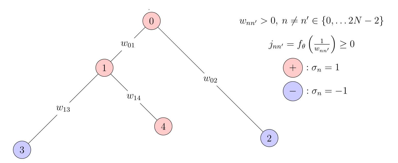
Figure 1. This phylogenetic tree $\mathcal{G}$ has $M_{o}=3$ leaf nodes, $M_{o}-1=2=M_{a}$ internal nodes and $2M_{o}-1=5=M_{tot}$ total nodes. Leaf nodes represent observed taxa, and internal nodes are unobserved ancestors. We observe a binary trait variable $\sigma_{m}$ for each of the leaf nodes and model all (both observed and unobserved) traits $\sigma_{m}$ using an Ising model with interactions $j_{mm^{\prime}}$ which condition on inferred weights $w_{mm^{\prime}}>0$.

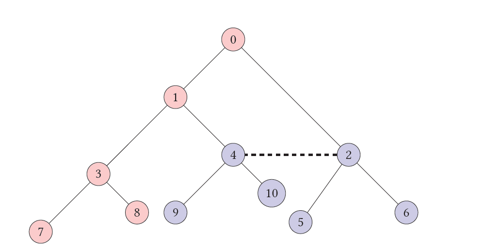
Figure 2. Reticulate evolution. This stylized bacterial phylogenetic network includes a reticulation (dashed line) that characterizes the exchange of genetic material between microbes. Whereas the network deviates from the bifurcating tree hypothesis of Figure 1, the problem of ancestral trait reconstruction is still meaningful.

Sampling algorithms are essential to the field of comparative phylogenetics, in general, and Bayesian phylogenetics (suchard2018bayesian, ), in particular. Here, we start with a fixed phylogenetic tree structure and the traits of observed biological specimens (Figure 1). We make the basic assumption that closely related taxa tend to share the same traits and establish a phylogenetic Ising model to predict the trait combinations of unobserved ancestors. We also adapt this model to deviations from the basic tree graph structure in the context of bacterial reticulate evolution and extend this model to incorporate multiple traits.

Specifically, suppose we assume a phylogenetic tree $\mathcal{G}$ (Fig 1) structure describes the shared evolutionary history giving rise to $M_{o}$ observed taxa indexed $m\in\{M_{o}-1,\dots,2M_{o}-1=M_{\text{tot}}\}$. This phylogenetic tree is a rooted, undirected, bifurcating and weighted graph that contains $M_{\text{tot}}=2M_{o}-1$ nodes, $M_{o}$ of which (corresponding to observed taxa) are leaf nodes, and $M_{a}=M_{o}-1$ are internal nodes. This graph also contains $2M_{o}-2$ edges, each of which has its own weight $w_{mm^{\prime}}>0$. If no edge exists between the node pair $m,m^{\prime}$, we say $w_{m,m^{\prime}}=\infty$. When edges exist, these weights are often proportional to the length of time spanning the existence of two organisms. Furthermore, suppose that we observe a binary trait $\sigma_{m}\in\{-1,1\}$ for each of our observed taxa. We then may use a simple Ising model (daskalakis2011evolutionary, ) to describe the joint distribution over observed and unobserved traits $\boldsymbol{\sigma}=(\sigma_{0},\dots,\sigma_{M_{\text{tot}}-1})$:

(9) $$Pr(\boldsymbol{\sigma}|\beta,\gamma,\mathcal{G})\propto\exp{\left(\beta\sum_{m,m^{\prime}}j_{mm^{\prime}}\sigma_{m}\sigma_{m^{\prime}}\right)},\quad\mbox{where}\quad j_{mm^{\prime}}=f_{\gamma}\left(\frac{1}{w_{mm^{\prime}}}\right)$$

and $\beta>0$, $f_{\gamma}:[0,\infty)\rightarrow[0,\infty)$, $f_{\gamma}(0)=0$ and $f_{\gamma}$ is an increasing function. For example, $f_{\gamma}(x)=\gamma\sqrt{x}$ for $\gamma>0$ is one of many possibilities. In the following, we treat $\gamma$ and $\beta$ as fixed, but one may learn them simultaneously with the rest of the model parameters in the context of Bayesian inference. From (9), we obtain the likelihood for the observed traits $\boldsymbol{\sigma}_{o}=(\sigma_{M_{a}},\dots,\sigma_{M_{\text{tot}}-1})$ by conditioning on unobserved ancestral traits $\boldsymbol{\sigma}_{a}=(\sigma_{0},\dots,\sigma_{M_{a}-1})$:

(10) $$Pr(\boldsymbol{\sigma}_{o}|\boldsymbol{\sigma}_{a},\beta,\gamma,\mathcal{G})\propto\exp{\left(\beta\sum_{m,m^{\prime}}j_{m,m^{\prime}}\sigma_{m}\sigma_{m^{\prime}}\right)}.$$

Placing the uniform prior on the ancestral traits $Pr(\boldsymbol{\sigma}_{a})\propto 1$, the posterior distribution for ancestral traits conditioned on observed traits becomes

(11) $$Pr(\boldsymbol{\sigma}_{a}|\boldsymbol{\sigma}_{o},\beta,\gamma,\mathcal{G})\propto Pr(\boldsymbol{\sigma}_{o}|\boldsymbol{\sigma}_{a},\beta,\gamma,\mathcal{G})\cdot Pr(\boldsymbol{\sigma}_{a})\propto\exp{\left(\beta\sum_{m,m^{\prime}}j_{m,m^{\prime}}\sigma_{m}\sigma_{m^{\prime}}\right)}.$$

Within the Bayesian paradigm of statistical inference (Gelman et al., 1995), the problem of inferring unobserved ancestral traits $\boldsymbol{\sigma}_{a}$ reduces to simulating from the Ising model (3) while keeping observed traits $\boldsymbol{\sigma}_{o}$ fixed. Note that it is relatively simple to infer the joint posterior $p(\boldsymbol{\sigma}_{a},\beta,\gamma|\boldsymbol{\sigma}_{o},\mathcal{G})$, although we do not consider this task here.

We build on this core model in two orthogonal ways. First, we consider the multi-trait scenario and model $T$ binary traits by allotting the $m$th specimen a spin of the form $\boldsymbol{\sigma}_{m}=(\sigma_{m,1},\dots,\sigma_{m,T})$. Following a development analogous to that of (9), (10) and (11), we specify a multi-trait phylogenetic Ising model that leads to the posterior distribution

(12) $$Pr(\boldsymbol{\sigma}_{a}|\boldsymbol{\sigma}_{o},\beta,\gamma,\mathcal{G})\propto\exp{\left(\beta\sum_{m,m^{\prime}}j_{m,m^{\prime}}\boldsymbol{\sigma}_{m}\cdot\boldsymbol{\sigma}_{m^{\prime}}\right)},$$

and $\boldsymbol{\sigma}_{a}=(\boldsymbol{\sigma}_{0},\dots,\boldsymbol{\sigma}_{M_{a}-1})$. Second, we consider failures of the bifurcating evolutionary tree hypothesis. Bacterial reticulate evolution (Figure 2) arises from the exchange of genetic material between microbes. In this context, it is appropriate to model evolution using a phylogenetic network. The Neighbor-net (neighborNet, ) algorithm is a popular algorithm for phylogenetic network construction that uses distances between genetic sequences to construct a planar splits graph. In this graph, extremal nodes are observed specimens, and interior nodes are potential ancestors. Whereas this evolutionary network model does not represent an explicit history of individual reticulations, it does represent conflicting signals regarding potential reticulations. These candidate reticulations take the form of the interior boxes that manifest in Figure 3.

On the one hand, using such a phylogenetic network as the base lattice structure in phylogenetic Ising models does not alter the mathematical details of the posterior distributions (11) and (12). On the other hand, the existence of cycles in the splits graph makes sampling these distributions significantly more difficult. (holbrook2023quantum, ) shows Algorithm 7’s potential for sampling from such challenging target distributions and advances QPMCMC, which approximately performs this algorithm. In the following, we present QPMCMC2 and its massive speedups over the $\mathcal{O}(P)$ complexity of Algorithm 2 and the $\mathcal{O}(\sqrt{P})$ complexity of QPMCMC.

3. Main Result: New Version of Quantum Parallel MCMC

In this section, we introduce our main result, which presents a novel quantum algorithm that surpasses Algorithm 2. Subsequently, we will delineate the technical contribution. Moreover, we will illustrate its significance in addressing the bottleneck identified in Algorithm 2. Finally, a comprehensive elucidation of our algorithm will be presented in detail.

Theorem 3.1.

There exists a quantum multiproposal Markov Chain Monte Carlo (MCMC) algorithm that takes inputs as detailed in Algorithm 2, with a running time:

$$\dfrac{2T(O_{\bar{q}})+T(O_{\pi})+\mathcal{O}(1)}{\min_{\alpha\in\mathcal{A}}(\pi(\boldsymbol{\theta}_{\alpha}))}.$$

Here, $O_{\bar{q}}$ and $O_{\pi}$ represent the quantum operations characterized by $\bar{q}(\boldsymbol{\theta},\boldsymbol{\theta}^{\prime})$ and $\pi(\cdot)$ respectively, which is irrelevant to number of the proposal P.

The primary technique relies on parallel computation within a quantum superposition state. In contrast to classical computers, quantum circuits allow us to prepare superposition states. When a unitary operation is applied to this superposition state, it simultaneously affects each state within the superposition. Building upon this foundational concept, it becomes evident that preparing a superposition state representing all $P$ proposals could enhance computation speed. This approach enables the simultaneous processing of calculations for various proposals.

3.1. Significance

3.1.1. Solving the Computation Bottleneck of Multiproposal MCMC

Previous studies have demonstrated the advantages of multiproposal MCMC algorithms over, e.g., the Metropolis-Hastings algorithm. Specifically, an increase in the number of proposals $P$ per Markov chain in Algorithm 2 leads to expedited convergence in the sampling process.

However, this accelerated convergence speed comes with a certain drawback. Typically, the bottleneck in each iteration of the Markov chain, as outlined in Algorithm 2, lies in the computation of $\pi$. The heightened number of $\pi_{p}$ computations required by this multiproposal MCMC algorithm demands significant computational resources when augmenting the proposal number $P$ per iteration. In Algorithm 2, achieving a single Markov chain iteration through classical computation necessitates a time complexity of $\mathcal{O}(P)$.

Conversely, a quantum circuit can execute parallel calculations across different proposals concurrently. This encompasses the generation of proposal sets, evaluation of $\pi_{p}$s and the selection of samples among them. This quantum approach holds promise in mitigating the bottleneck of the multiproposal MCMC algorithm, thereby expediting the convergence process. By concurrently processing multiple proposals, this quantum multiproposal MCMC algorithm becomes more competitive in comparison to traditional algorithms that relie on a single proposal.

3.1.2. Comparison with State of the Art Quantum Algorithm

In reality, this work is not the first to utilize quantum circuits in an endeavor to expedite Algorithm 2. In a prior investigation conducted by Holbrook (holbrook2023quantum, ), the employment of the Grover search approach and the Gumbel-Max trick aimed to devise a quantum algorithm (QPMCMC) for substituting lines 3-4 in  Algorithm 2, thereby enhancing the time complexity of these steps from $\mathcal{O}(P)$ to $\mathcal{O}(\sqrt{P})$. It is noteworthy that, in that study, the acceleration did not extend to the process of generating $P$ proposal sets (line 2, Algorithm 2), maintaining the overall complexity for a QPMCMC iteration at $\mathcal{O}(P)$.

Upon comparing this work to the previously mentioned study, it becomes evident that our approach signifies a notable advancement over the state-of-the-art work. We achieve an exponential speedup in terms of the proposal count $P$ when contrasted with Algorithm 2.

3.2. A Quantum Parallel MCMC and its time complexity

Algorithm 3 Quantum accelerated multiproposal MCMC (QPMCMC2)

1:An initial Markov chain state $\boldsymbol{\theta}^{(0)}$; an oracle $O_{\pi}$ for evaluating target distribution $\pi(\cdot)$; an oracle $O_{\bar{q}}$ for sampling $\boldsymbol{\theta}^{\prime}$ from a Tjelmeland distribution $\bar{q}(\boldsymbol{\theta},\boldsymbol{\theta}^{\prime})$ symmetric in $\boldsymbol{\theta}$ and $\boldsymbol{\theta}^{\prime}$; a control rotation operator $R(\theta)$; the number of samples to generate $S$; the number of proposals $P$.

2:for $s\in{1,\ldots,S}$ do

3:     Prepare a quantum state $\ket{\psi_{0}}=\ket{0}_{\mathcal{P}}\ket{0}_{\mathcal{H}_{0}}\ket{0}_{\mathcal{H}_{1}}\ket{0}_{\mathcal{H}_{2}}\ket{0}_{\Pi}\ket{0}_{S}$

4:     Encode $\boldsymbol{\theta}^{(s-1)}$ in $\mathcal{H}_{0}$.

5:     Apply $O_{\bar{q}}$, which takes query from $\mathcal{H}_{0}$ and responses in $\mathcal{H}_{1}$

6:     Make a uniform superposition state in $\mathcal{P}$

7:     Apply $O_{\bar{q}}$, which takes a query from $\mathcal{H}_{1}$, and responses in $\mathcal{H}_{2}$ on each state

8:     Apply $O_{\pi}$, which takes a query from $\mathcal{H}_{2}$, and responses in $\Pi$ on each state

9:     Apply a control rotation gate $R$ (controlled by each $\ket{p}_{\mathcal{P}}$), which takes a query from $\Pi$ and

10:     maps $\ket{0}_{\mathcal{S}}$ to $\sqrt{1-\pi(\boldsymbol{\theta}_{p})}\ket{0}_{S}+\sqrt{\pi(\boldsymbol{\theta}_{p})}\ket{1}_{S}$

11:     Make a measurement;

12:     if $\mathcal{S}$ register is $0$ then: restart form line 3.

13:     end if

14:     $\boldsymbol{\theta}^{(s)}\leftarrow$ the data in $\mathcal{H}_{2}$

15:end for

16:return $\boldsymbol{\theta^{(1)}},\ldots,\boldsymbol{\theta^{(S)}}$.

In this subsection, we initially provide a detailed description of a quantum parallel MCMC algorithm (Algorithm 3). Subsequently, we establish its correctness and analyze its time complexity.

Algorithm 3 takes the following inputs: An initial Markov chain state $\boldsymbol{\theta}_{0}$, the number of samples to generate $S$, and the number of proposals $P$. The implementation of Algorithm 3 also necessitates the oracles $O_{\bar{q}}$ and $O_{\pi}$, which simulate classical functions $\bar{q}(\boldsymbol{\theta},\boldsymbol{\theta}^{\prime})$ and $\pi(\cdot)$ used in Algorithm 2, respectively. Furthermore, it requires a rotation operation $R$. These quantum operations are defined in Section 2.3.2.

The quantum algorithm begins by initializing several quantum registers according to the following scheme:

• The first register, denoted as $\mathcal{P}$, is encoded with the labels of proposals $\{0,\cdots,P\}$ as specified in Algorithm 2.

• The second register, labeled $\mathcal{H}_{0}$, is encoded with the selected state $\boldsymbol{\theta}^{(s-1)}$ from the preceding Markov chain.

• The third register, termed $\mathcal{H}_{1}$, is encoded with the random offset $\bar{\boldsymbol{\theta}}$ as described in Algorithm 2.

• The fourth register, denoted as $\mathcal{H}_{2}$, is encoded with the proposals $\boldsymbol{\theta}_{p}\stackrel{{\scriptstyle i.i.d.}}{{\sim}}\bar{q}(\boldsymbol{\theta},\boldsymbol{\theta}^{\prime})$ for each label of proposal $p\in\{0,\cdots,P\}$.

• The fifth register, denoted as $\Pi$, is encoded with the evaluated value from the target distribution $\pi(\cdot)$ for each label of proposal $p$.

• The last register, designated as $\mathcal{\mathcal{S}}$, is a register indicating whether the implementation of the Markov chain is successful or not.

For the $s^{\text{th}}$ Markov chain iteration, the quantum algorithm commences by initializing these quantum registers to hold zero and subsequently executing five steps.

Initially, Algorithm 3 encodes the initial Markov chain state $\boldsymbol{\theta}_{0}$, defined as the selected state $\boldsymbol{\theta}^{(s-1)}$ from the preceding Markov chain, into the register $\mathcal{H}_{0}$. This operation necessitates approximately $\mathcal{O}(\log(|\mathcal{A}|))$ controlled-NOT gate operations where $\mathcal{A}$ is the parameter space (introduced in Section 2.1).

Secondly, Algorithm 3 considers an operator $O_{\bar{q}}$ characterized by the proposal distribution $\bar{q}(\boldsymbol{\theta}_{0},\cdot)$. This operation selects a state $\bar{\boldsymbol{\theta}}$ from the distribution $\bar{q}(\boldsymbol{\theta}_{0},\cdot)$ and encodes this state into the register $\mathcal{H}_{1}$. The resulting state is represented as:

$$\ket{0}_{\mathcal{P}}\ket{\boldsymbol{\theta}^{(s-1)}}_{\mathcal{H}_{0}}\ket{\bar{\boldsymbol{\theta}}}_{\mathcal{H}_{1}}\ket{0}_{\mathcal{H}_{2}}\ket{0}_{\Pi}\ket{0}_{S},$$

where $\bar{\boldsymbol{\theta}}\sim\bar{q}\left(\boldsymbol{\theta}_{0},\cdot\right)$. The time required for this step is $T(O_{\bar{q}})$.

Thirdly, Algorithm 3 creates a uniformly distributed superposition in register $\mathcal{P}$ such that each state is entangled with the proposal states $\boldsymbol{\theta}_{p}$ encoded in register $\mathcal{H}_{2}$. This process can be achieved by employing approximately $\mathcal{O}(\log(P))$ Hadamard gate operations on register $\mathcal{P}$, followed by an operation $O_{\bar{q}}$ controlled by each $\ket{p}_{\mathcal{P}}$. This operation receives a query from $\mathcal{H}_{1}$ and responds in $\mathcal{H}_{2}$. The resultant state is given by:

$$\frac{1}{\sqrt{P+1}}\sum_{p=0}^{P}\ket{p}_{\mathcal{P}}\ket{\boldsymbol{\theta}^{(s-1)}}_{\mathcal{H}_{0}}\ket{\bar{\boldsymbol{\theta}}}_{\mathcal{H}_{1}}\ket{\boldsymbol{\theta}_{p}}_{\mathcal{H}_{2}}\ket{0}_{\Pi}\ket{0}_{S},$$

where $\boldsymbol{\theta}_{1},\ldots,\boldsymbol{\theta}_{P}\stackrel{{\scriptstyle i.i.d.}}{{\sim}}\bar{q}(\bar{\theta},\cdot)$. It’s important to note that the time complexity for this operation is $T(O_{\bar{q}})+\mathcal{O}(1)$.

The fifth step involves encoding the evaluated value from the target distribution $\pi(\cdot)$ for each proposal label into the prefactor of each state. This task comprises two operations: the first is an oracle $O_{\pi}$ that accepts queries from $\mathcal{H}_{2}$ and responds with the answer in the $\Pi$ register. Subsequently, a controlled rotation operator $R$ receives a query from $\Pi$ and rotates the qubit in $\mathcal{S}$. The resulting state is expressed as:

$$\frac{1}{\sqrt{P+1}}\sum_{p=0}^{P}\ket{p}_{\mathcal{P}}\ket{\boldsymbol{\theta}^{(s-1)}}_{\mathcal{H}_{0}}\ket{\bar{\boldsymbol{\theta}}}_{\mathcal{H}_{1}}\ket{\boldsymbol{\theta}_{p}}_{\mathcal{H}_{2}}\ket{\pi(\boldsymbol{\theta}_{p})}_{\Pi}\left(\sqrt{1-\pi(\boldsymbol{\theta}_{p})}\ket{0}_{S}+\sqrt{\pi(\boldsymbol{\theta}_{p})}\ket{1}_{S}\right).$$

The time complexity of this task is $T(O_{\pi})+\mathcal{O}(1)$.

In the final step, Algorithm 3 executes two measurements: the initial measurement targets the $\mathcal{S}$ register, followed by a subsequent measurement on the $\mathcal{H}_{2}$ register. Should the qubit within the $\mathcal{S}$ register yield a state of $1$, the resultant state is altered to:

$$\sum_{p^{\prime}=0}^{P}\sqrt{\frac{\pi(\boldsymbol{\theta}_{p})}{\sum_{p^{\prime}=0}^{P}\pi(\boldsymbol{\theta}_{p^{\prime}})}}\ket{p}_{\mathcal{P}}\ket{\boldsymbol{\theta}^{(s-1)}}_{\mathcal{H}_{0}}\ket{\bar{\boldsymbol{\theta}}}_{\mathcal{H}_{1}}\ket{\boldsymbol{\theta}_{p}}_{\mathcal{H}_{2}}\ket{\pi(\boldsymbol{\theta}_{p})}_{\Pi}\ket{1}_{S}.$$

Subsequently, Algorithm 3 performs a measurement on the $\mathcal{H}_{2}$ register, denoting the outcome as $\boldsymbol{\theta}^{(s)}$, representing the selected state in the $s^{\text{th}}$ Markov chain. Next, we give a proof of Theorem 3.1.

Proof.

The correctness of this process follows from the correctness of Algorithm 2 if the register $\mathcal{S}$ holds the qubit $1$. Therefore, the time complexity is the summation of the time complexity described above multiplied by $1/R$, where $R$ is the probability of the event that the measurement in the register $\mathcal{S}$ yields $1$, which is lower bounded as follows:

(13) $$R=\frac{\sum_{p^{\prime}=0}^{P}\pi(\boldsymbol{\theta}_{p^{\prime}})}{P+1}\geq\min_{p\in\{0,\cdots,P\}}(\pi(\theta_{p}))\geq\min_{\boldsymbol{\theta}\in\mathcal{A}}(\pi(\boldsymbol{\theta})),$$

where $\mathcal{A}$ is the parameter space, and the last inequality uses the fact that $\{\boldsymbol{\theta}_{p}\}_{p=0}^{P}\subset\mathcal{A}$. It’s noteworthy that this lower bound is independent of the number of proposals $P$. Consequently, Theorem 3.1 follows. ∎

4. Case Study: Inferring Traits On a Phylogenetic Network

The learning of ancestral traits (Section 2.4) within a known phylogenetic network illustrates our algorithm’s speed, flexibility and fully-explicit nature. Consider a phylogenetic network $\mathcal{G}(V,E)$, where $V$ denotes a set of $M_{\text{tot}}$ vertices and $E$ represents a set of edges. Let $V_{o}$ be a designated subset of $V$ signifying the observed taxa within this context, and $V_{a}=V\backslash V_{o}$ be the complement set of $V_{o}$. For the network shown in Figure 2, we have $M_{tot}=|V|=11$, $V_{o}=\{5,\dots,10\}$ and $V_{a}=\{0,\dots,4\}$. Using the notation of Sections 2.1, 2.2 and 3, we identify any Markov chain state with a collection of ancestral traits thus:

(14) $$\boldsymbol{\theta}=(\boldsymbol{\sigma}_{0},\boldsymbol{\sigma}_{1},\ldots,\boldsymbol{\sigma}_{{M_{a}}-1})\,,$$

where $\boldsymbol{\sigma}_{m}=(\sigma_{m,1},\ldots,\sigma_{m,T})$ for $\sigma_{m,t}\in\{-1,1\}$. Assuming that each $(m,m^{\prime})\in E$ possesses an identical weight $J$, we rewrite the posterior (12) as

(15) $$Pr(\boldsymbol{\sigma}_{a}|\boldsymbol{\sigma}_{o},J,\mathcal{G})\propto\exp\left\{J\sum_{(m,m^{\prime})\in E}\boldsymbol{\sigma}_{m}\cdot\boldsymbol{\sigma}_{m^{\prime}}\right\}\quad\mbox{and set}\quad\pi(\boldsymbol{\theta}):=Pr(\boldsymbol{\sigma}_{a}|\boldsymbol{\sigma}_{o},J,\mathcal{G})\,.$$

Fixing the observed traits and sampling unobserved ancestral traits using QPMCMC2 amounts to efficient posterior inference.

In the following, we specify the Tjelmeland kernel $\bar{q}(\cdot,\cdot)$ and detail the target distribution $\pi(\cdot)$ for the phylogenetic Ising model. Next, we analyze the qubit requirements when applying Algorithm 3 for this specific inferential task. Finally, the acceptance rate $R$ of Algorithm 3 in this application scenario is introduced.

4.1. Tjelmeland kernel $\bar{q}(\cdot,\cdot)$

We specify the symmetric Tjelmeland kernel $\bar{q}(\cdot,\cdot)$ by defining the distribution $\bar{q}(\boldsymbol{\theta},\cdot)$ centered at a generic state (14). For each $t\in\{1,\dots,T\}=\mathcal{T}$ and $m\in\{0,\dots,M_{a}-1\}=V_{a}$, we define the result state

(16) $$\boldsymbol{\theta}_{m,t}=(\boldsymbol{\sigma}_{0},\ldots\boldsymbol{\sigma}_{m}^{\prime},\ldots,\boldsymbol{\sigma}_{M_{a}-1}),$$

where $\boldsymbol{\sigma}_{m}^{\prime}=(\sigma_{m,1},\ldots-\sigma_{m,t},\ldots,\sigma_{m,T})$. The vectors $\boldsymbol{\theta}$ and $\boldsymbol{\theta}_{m,t}$ only differ by a negative sign at the trait $(t,m)$. Since there are $M_{a}T=(M_{\text{tot}}-M_{o})T$ possibilities of $\boldsymbol{\theta}_{m,t}$, we write down $\bar{q}(\boldsymbol{\theta},\boldsymbol{\theta}^{\prime})$ formally as

(17) $$\bar{q}(\boldsymbol{\theta},\boldsymbol{\theta}^{\prime})=\begin{cases}\frac{1}{M_{a}T+1}&\text{if }\boldsymbol{\theta}^{\prime}\in\boldsymbol{\Theta}\\ 0&\text{otherwise}\,,\end{cases}$$

where $\boldsymbol{\Theta}=\{\boldsymbol{\theta}_{m,t}:t\in\mathcal{T}\text{ and }m\in V_{a}\}\cup\{\boldsymbol{\theta}\}$. In words, $\bar{q}(\boldsymbol{\theta},\cdot)$ is a uniform distribution over the nearest neighbors to $\boldsymbol{\theta}$ and $\boldsymbol{\theta}$ itself.

4.2. Target function $\pi(\cdot)$

When using the Tjelmeland distribution (17) within Algorithm 3, each proposal state $\boldsymbol{\theta}_{p}$ has at most one trait that is different from the intermediate state $\bar{\boldsymbol{\theta}}$. We can, therefore, derive a simpler form of the function $\pi(\cdot)$ for such proposals.

(20) $$\pi_{p}\propto\frac{\pi(\boldsymbol{\theta}_{p})}{\pi(\bar{\boldsymbol{\theta}})}=\left\{\begin{array}[]{cc}\exp{-2J\sum_{m;(m,m_{p})\in E}\bar{\sigma}_{m_{p},t_{p}}\cdot\bar{\sigma}_{m,t_{p}}}&\text{if }\boldsymbol{\theta}_{p}\neq\bar{\boldsymbol{\theta}}\\ 1&\text{otherwise}\,,\end{array}\right.$$

where the $(m_{p},t_{p})$ are the flipped trait in proposal $p$, and the $\bar{\sigma}_{m,t_{p}}$ represent the $t_{p}^{\text{th}}$ trait spin of vertex $m$ adjacent to proposed vertex $m_{p}$ in the intermediate state $\bar{\boldsymbol{\theta}}$.

But we need to refine this representation in order to use it within Algorithm 3. We must ensure that each $\pi_{p}$ inhabits the domain $\text{[}0,1\text{]}$. Therefore, the above equation is multiplied by a factor $\exp(\text{deg}(\mathcal{G}))$, then Eq. 20 becomes $\pi_{p}=\exp{-2Jf(m_{p},t_{p};\bar{\boldsymbol{\theta}})}$ where

(21) $$f(m_{p},t_{p};\bar{\boldsymbol{\theta}})=\begin{cases}\sum_{m;(m,m_{p})\in E}\bar{\sigma}_{m_{p},t_{p}}\cdot\bar{\sigma}_{m,t_{p}}+\text{deg}(\mathcal{G})&\text{if }\boldsymbol{\theta}_{p}\neq\bar{\boldsymbol{\theta}}\\ \text{deg}(\mathcal{G})&\text{otherwise}\,,\end{cases}$$

We observe that $f(m_{p},t_{p};\bar{\boldsymbol{\theta}})\geq 0$, and that each $\pi_{p}$ satisfies $0\leq\pi_{p}\leq 1$ which enables the implementing line $9$ in Algorithm 3.

4.3. Circuit reduction

By giving the specific form of functions $\bar{q}(\cdot)$ and $\pi(\cdot)$, we are already able to construct full circuit for Algorithm 2 and Algorithm 3. Here, we want to provide a furthur reduction on resources when we implementing this algorithm in this Ising model sampling problem.

First, from the inspiration of Eq. 21, we see that $\pi_{p}$ is determined by $f(m_{p},t_{p};\bar{\boldsymbol{\theta}})$. With this idea, we could replace $\boldsymbol{\theta}_{p}$ with a pair of number $(m_{p},t_{p})$ that describe the trait we’re flipping $(m_{p},t_{p})$ from the intermediate state $\bar{\boldsymbol{\theta}}$ forming the proposal state. Thus the qubits requirement for the register $\mathcal{H}_{2}$ in Algorithm 3 can be reduced from $\lceil TM_{a}log_{2}(TM_{a})\rceil$ to $\lceil log_{2}(TM_{a})\rceil$.

Next, notice that we’re able to avoid the calculation of function $\pi(\cdot)$ in this trait inferring problem. When it comes to computing $\pi_{p}$ in Algorithm 3, although it is theoretically available for us to construct an quantum oracle that calculate this exponential function (21) from known $f(t_{p},m_{p};\bar{\boldsymbol{\theta}})$, it is relatively hard for nowadays quantum device to do it. Hopefully, due to the fact that the degree of the phylogenetic network $\mathcal{G}$ is small in practical applications, the number of the possibilities of $\pi_{p}$, which is $2\text{deg}(\mathcal{G})+1$, is also limited. Therefore, we could encode these $\pi_{p}$ on one lookup table in advance, which consumes $O(\text{deg}(\mathcal{G}))$ time complexity, then $\pi(\boldsymbol{\theta}_{p})$ can be calculated by this table. This reduction avoid the calculation in Eq. 21 for each proposal and for each Markov chain.

These two reductions are applicable in both Algorithm 2 and Algorithm 3. It’s worth noting that these reductions do not notably reduce the scale of time and space complexity, thus may not be significant on classical computers. However, they are crucial for implementation on quantum computers. Given the current scarcity and noisy nature of qubits, the requirements for depth and space in quantum algorithms that can be practically implemented are extremely stringent. In fact, few quantum devices have more than thousands of qubits, yet in many phylogenetic graphs, $M_{tot}$ can easily exceed ten thousands. Furthermore, computing complicated functions is still a challenge on current noisy quantum devices, whereas a one to one corresponding rotation gate are relatively much simpler. These two reductions significantly reduce the qubits requirement and the depth of the quantum circuit, making Algorithm 3 more viable for practical implementation.

4.4. Acceptance rate analysis for sampling Ising model

In this section, we will provided further discussion about the acceptance rate $R_{\text{Ising}}$ when sampling state according to Ising model based on this tree graph $\mathcal{G}(V,E)$.

Theorem 4.1.

Let the previous state be $\boldsymbol{\theta}_{0}$. $T$ is the number of traits and $M_{\text{tot}}$ is the number of vertices in $\mathcal{G}$. For a large number of proposal $P$ and a large number of traits $TM_{\text{tot}}$, if the number of taxa vertices $M_{a}<<M_{tot}$, the approximate lower bound for $E(R_{\text{Ising}})$ is $Pr(\boldsymbol{\theta}_{0})^{{-4/TM_{\text{tot}}}}\cdot e^{-2J\text{deg}(\mathcal{G})}$, which can be further bounded by lower bound $e^{-4J\text{deg}(\mathcal{G})}$.

Proof.

Now we start the proof of theorem 4.1. In our cases, we have relative possibility of each proposal as

(22) $$\pi_{p}=e^{-2Jf(m_{p},t_{p};\bar{\boldsymbol{\theta}})},\text{ where }f(m_{p},t_{p};\bar{\boldsymbol{\theta}})=\sum_{m;(m,m_{p})\in E}\bar{\sigma}_{m_{p},t_{p}}\cdot\bar{\sigma}_{t_{p},m}+deg(\mathcal{G}).$$

First observe that $0\leq f(m_{p},t_{p})\leq 2\text{deg}(\mathcal{G})$. Based on the acceptance rate analysis of general QPMCMC (13), we have a more tight lower bound for this trait inferring problem. When generating $(m_{p},t_{p})$ for each proposal, we randomly draw traits uniformly over the graph and over all traits through the given $\bar{q}$. Utilizing the above equation, we can further calculate the average of $R_{\text{Ising}}$ among all cases selecting different combinations of proposals in each iteration as

(23) $$E(R_{\text{Ising}})=\frac{\sum_{t\in\mathcal{T}}\sum_{m\in V_{a}\pi_{(t,m)}}}{TM_{a}}(P/P+1)+\pi_{t_{0},m_{0}}(1/(P+1)),$$

where $\pi_{(t,m)}=e^{-2Jf(t,m;\bar{\boldsymbol{\theta}})}$. Notice that we care more about the cases of a large $P$, so we could have $P/(P+1)\sim 1$ and $1/(P+1)\sim 0$. Also, for a graph $\mathcal{G}$, if the fixed taxas $M_{a}<<M_{\text{tot}}$, the vertices set $V_{o}\sim V$. Combining the mentioned condition, with the AM-GM inequality, we could have the approximate lower bound of $R_{\text{Potts}}$ as

(24) $$E(R_{\text{Ising}})\approx\frac{\sum_{t=1}^{T}\sum_{m=0}^{M_{\text{tot}}-1}\pi_{(t,m)}}{TM_{\text{tot}}}\geq(e^{-2J\sum_{t=1}^{T}\sum_{m=0}^{M_{\text{tot}}-1}f(t,m;\bar{\boldsymbol{\theta}})})^{1/TM_{\text{tot}}}.$$

Notice that from (22), $f(t,m;\bar{\boldsymbol{\theta}})$ are considering all edges around vertices $(t,m)$, so summing over all vertices among the graph would result in counting the contribution of all edges twice. Inspiring with this thoughts, we are able to link $f(t,m;\bar{\boldsymbol{\theta}})$ with $Pr({\boldsymbol{\theta}})$ described in (Eq. 12) as

(25) $$(e^{-2J\sum_{t=1}^{T}\sum_{m=0}^{M_{\text{tot}}-1}f(t,m;\bar{\boldsymbol{\theta}})})=e^{-2JTM_{\text{tot}}\text{deg}(\mathcal{G})}\cdot Pr(\bar{\boldsymbol{\theta}})^{4}.$$

For a large amount of traits $TM_{\text{tot}}>>1$, we could make a reasonable approximation that $Pr(\bar{\boldsymbol{\theta}})$ $\sim$ $Pr(\boldsymbol{\theta}_{0})$. Now we could rewrite the lower bound with

(26) $$E(R_{\text{Ising}})\approx\frac{\sum_{t=1}^{T}\sum_{m=0}^{M_{\text{tot}}-1}\pi_{(t,m)}}{TM_{\text{tot}}}\geq Pr(\boldsymbol{\theta}_{0})^{{-4/TM_{\text{tot}}}}\cdot e^{-2J\text{deg}(\mathcal{G})}\geq e^{-4J\text{deg}(\mathcal{G})}.$$

We can see that the expected acceptance rate $E(R_{\text{Ising}})$ depends on the probability of the intermediate state $Pr(\bar{\boldsymbol{\theta}})$, which is very closed to the previous sampled state $Pr(\boldsymbol{\theta}_{0})$. While the sampling process converged at a higher probability state, the lower bound of $E(R_{\text{Ising}})$ decreased, but still greater than the general bound $e^{-4J\text{deg}(\mathcal{G})}$. Notice that these bounds are still independent of proposal number $P$, but it do cause implementing problems when the $J$ is large.

∎

5. Application: salmonella and antibiotic resistance

Conditioning on antibacterial drug resistance scores for 248 salmonella bacterial isolates, we apply our QPMCMC2 to the Bayesian inference of ancestral traits on a Neighbor-net phylogenetic network (Section 2.4). (mather2013distinguishable, ; cybis2015assessing, ) previously use this biological sample to analyze the development of antibiotic resistances within the genus salmonella but do not account for bacterial reticulate evolution. Our phylogenetic network, denoted as $\mathcal{G}_{\text{sal}}(V,E)$, comprises $M_{tot}=3{,}313$ vertices with $|E|=5{,}945$ edges. Among all the vertices, there are $M_{o}=248$ observed taxa, representing the observed biological isolates with known traits. Pertinent to the theoretical developments of Section 4, the degree of our network is deg$(\mathcal{G}_{\text{sal}})=8$. In this section, we use a classical simulator to execute Algorithm 3 and ascertain its efficiency. We apply our algorithm to two separate cases, the single-trait case $T=1$ and the multi-trait case $T=4$.

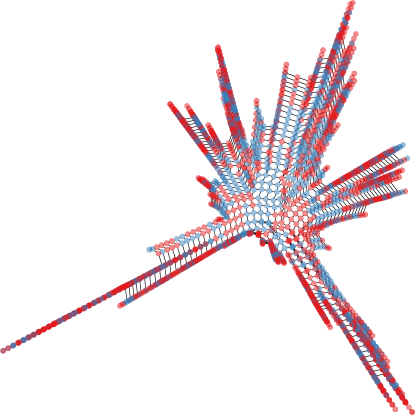
Figure 3. A Neighbor-net phylogenetic network describes the shared evolutionary history of 248 salmonella bacteria. The extremal nodes correspond to the 248 observed isolates, and the $M_{a}=3{,}065$ interior nodes correspond to unobserved ancestors. Interior squares are potential reticulation events. Colors (red, resistance; blue, no resistance) are observed and posterior mode resistances to the antibiotic ampicillin for observed microbes and unobserved ancestors, respectively.

We use ampicillin resistance as the binary trait for the single-trait experiment. We set the initial state as $\boldsymbol{\theta}_{0}=(\sigma_{0},\ldots,\sigma_{M_{a}-1})$, with ancestral traits set to $\sigma_{m}=(-1)^{m}$. Starting from this initial state, we apply QPMCMC2  with various proposal numbers $P$ to sample ancestral traits. Figure 3 shows node-specific posterior modes obtained using 150,000 MCMC iterations with proposal count $P=128$. The modes correspond to the final 130,000 samples thinned at a rate of 500 to 1. From the relationships shows in the plot (a) of (Fig. 4), it is evident that by calculating more proposals in a single iteration, QPMCMC2 converges faster and is capable of converging to a significantly higher-probability states. This demonstrates the value of the algorithm: in our approach, by replacing Algorithm 2 with Algorithm 3, we are able to compute in parallel all $P$ proposals with $O(\log P)$ qubits during each iteration. With the help of quantum computing, multiproposal MCMC has a better chance to outperform the traditional single proposal MCMC algorithm such as Metropolis-Hastings or Barker’s algorithm (Algorithm 1). We also apply QPMCMC2 to a phylogenetic network Ising model with multiple traits (ampicillin, chloramphenicol, ciprofloxacin and furazolidone resistances). Plot (b) in Fig. 4 shows the trace plot for the corresponding log-posterior $T=4$. When the number of the parallel proposals $P$ increases, the ancestral trait configuration also tends to converge to states with higher posterior probabilities according to Eq. 12. As one might expect, the algorithm seems to require $T$ times the number of iterations required when $T=1$.

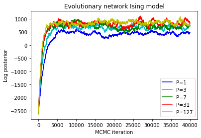
(a) Single-trait Ising model traces

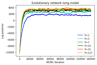
(b) Four-trait Ising model traces

Figure 4. Trace plots generated by the QPMCMC2 algorithm for different numbers of proposals $P$. For both the single-trait and multi-trait problem, increasing $P$ accelerates convergence to higher posterior probability states. Better still, the QPMCMC2 algorithm pays no penalty for the use of additional proposals (Figure 5).

Another important indicator of sampling efficiency is the effective sample size (ESS):

$$\mbox{ESS}:=\frac{S}{\sum_{s=-\infty}^{\infty}\rho(s)}\,,$$

where $S$ is the number of MCMC samples, and $\rho(s)$ is the autocorrelation of a univariate time series at lag $s$. An effective sampler generally exhibits lower autocorrelation for key model summary statistics, resulting in a larger ESS. The ESS provides a measure of how many independent samples the correlated chain is equivalent to: it gives you an idea of the true amount of information your sample contains, taking into account the correlation between sample points. We estimate ESS using the Python package ArviZ (kumar2019arviz, ). Fig. 5 shows that the ESS per 10k oracles is increased when we use a larger proposal count $P$ for QPMCMC2. The same is not true for the classical PMCMC (Algorithm 2). Almost every quantum oracle we use in our implementation is the quantum equivalent of the corresponding classical operator. The only difference is that during each iteration, QPMCMC2 requires reruns and the PMCMC requires $P$ times the number of oracle calls since it evaluates the target at each proposal separately. In Fig. 4, we can see that when the $P$ increases, we obtain a larger ESS using QPMCMC2  per oracles due to quantum parallelism.

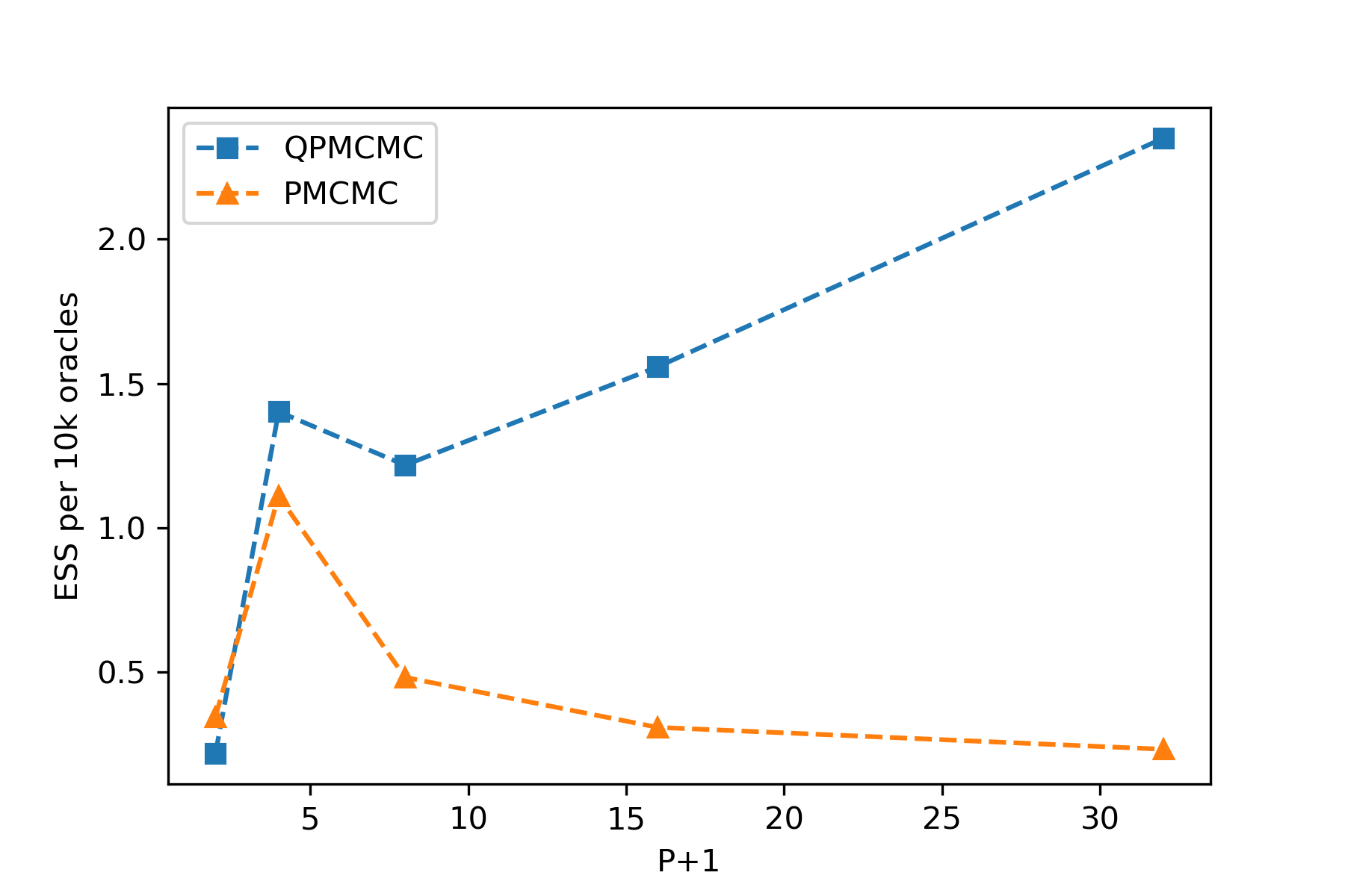
Figure 5. Effective sample size (ESS) for the log posterior per 10,000 oracle calls for different numbers of proposals $P$. Since QPMCMC2 pays no penalty for additional proposals $P$, it does not exhibit the decreasing performance suffered by the classical implementation (PMCMC).

In both the single- and the multi-trait experiment, we can observe the advantage of having a large proposal count $P$ when applying multiproposal MCMC in the convergence process. This highlights two major strengths of the quantum algorithm we propose:

1. Making an exponential speed up. For large $P$ in multiproposal MCMC algorithms, we can reduce the dependence of $P$ of the time complexity from $\mathcal{O}(P)$ to $\mathcal{O}(1)$ with $\mathcal{O}(\log(P))$ ancillary qubits. This is an exponential speed up for the dependence of $P$ which solves the bottleneck of the original Algorithm 2.

2. Accelerated sampling for real-world problems. We have demonstrated the benefits for our quantum algorithm in accelerating sampling for a realistic and non-trivial class of graphical models. This quantum algorithm shows the potential to accelerate Bayesian inference for this important problem in biomedicine.

References

- [1] Hakon Tjelmeland. Using all metropolis–hastings proposals to estimate mean values. Technical report, 2004.
- [2] Daan Frenkel. Speed-up of monte carlo simulations by sampling of rejected states. Proceedings of the National Academy of Sciences, 101(51):17571–17575, 2004.
- [3] Jean-Françcois Delmas and Benjamin Jourdain. Does waste recycling really improve the multi-proposal metropolis–hastings algorithm? an analysis based on control variates. Journal of applied probability, 46(4):938–959, 2009.
- [4] Radford M Neal. Mcmc using ensembles of states for problems with fast and slow variables such as gaussian process regression. arXiv preprint arXiv:1101.0387, 2011.
- [5] Ben Calderhead. A general construction for parallelizing metropolis- hastings algorithms. Proceedings of the National Academy of Sciences, 111(49):17408–17413, 2014.
- [6] Xin Luo and Håkon Tjelmeland. A multiple-try metropolis–hastings algorithm with tailored proposals. Computational Statistics, 34(3):1109–1133, 2019.
- [7] Nicholas Metropolis, Arianna W Rosenbluth, Marshall N Rosenbluth, Augusta H Teller, and Edward Teller. Equation of state calculations by fast computing machines. The journal of chemical physics, 21(6):1087–1092, 1953.
- [8] W. K. Hastings. Monte Carlo sampling methods using Markov chains and their applications. Biometrika, 57(1):97–109, 04 1970.
- [9] Nathan E Glatt-Holtz, Andrew J Holbrook, Justin A Krometis, and Cecilia F Mondaini. Parallel mcmc algorithms: Theoretical foundations, algorithm design, case studies. arXiv preprint arXiv:2209.04750, 2022.
- [10] Andrew J Holbrook. Generating mcmc proposals by randomly rotating the regular simplex. Journal of Multivariate Analysis, 194:105106, 2023.
- [11] Andrew J Holbrook. A quantum parallel markov chain monte carlo. Journal of Computational and Graphical Statistics, pages 1–14, 2023.
- [12] Christoph Durr and Peter Hoyer. A quantum algorithm for finding the minimum. arXiv preprint quant-ph/9607014, 1996.
- [13] Theodore J Yoder, Guang Hao Low, and Isaac L Chuang. Fixed-point quantum search with an optimal number of queries. Physical review letters, 113(21):210501, 2014.
- [14] Lov K Grover. A fast quantum mechanical algorithm for database search. In Proceedings of the twenty-eighth annual ACM symposium on Theory of computing, pages 212–219, 1996.
- [15] Luke Tierney. Markov chains for exploring posterior distributions. the Annals of Statistics, pages 1701–1728, 1994.
- [16] Joseph Felsenstein. Phylogenies and the comparative method. The American Naturalist, 125(1):1–15, 1985.
- [17] Gabriel W Hassler, Andrew F Magee, Zhenyu Zhang, Guy Baele, Philippe Lemey, Xiang Ji, Mathieu Fourment, and Marc A Suchard. Data integration in bayesian phylogenetics. Annual Review of Statistics and Its Application, 10:353–377, 2023.
- [18] Zhenyu Zhang, Akihiko Nishimura, Paul Bastide, Xiang Ji, Rebecca P Payne, Philip Goulder, Philippe Lemey, and Marc A Suchard. Large-scale inference of correlation among mixed-type biological traits with phylogenetic multivariate probit models. The Annals of Applied Statistics, 15(1):230–251, 2021.
- [19] Zhenyu Zhang, Akihiko Nishimura, Nidia S Trovao, Joshua L Cherry, Andrew J Holbrook, Xiang Ji, Philippe Lemey, and Marc A Suchard. Accelerating bayesian inference of dependency between mixed-type biological traits. PLOS Computational Biology, 19(8):e1011419, 2023.
- [20] David Bryant and Vincent Moulton. Neighbor-Net: An Agglomerative Method for the Construction of Phylogenetic Networks. Molecular Biology and Evolution, 21(2):255–265, 02 2004.
- [21] AE Mather, SWJ Reid, DJ Maskell, J Parkhill, MC Fookes, SR Harris, DJ Brown, JE Coia, MR Mulvey, MW Gilmour, et al. Distinguishable epidemics of multidrug-resistant salmonella typhimurium dt104 in different hosts. Science, 341(6153):1514–1517, 2013.
- [22] Gabriela B Cybis, Janet S Sinsheimer, Trevor Bedford, Alison E Mather, Philippe Lemey, and Marc A Suchard. Assessing phenotypic correlation through the multivariate phylogenetic latent liability model. The annals of applied statistics, 9(2):969, 2015.
- [23] Andrew Gelman, John B Carlin, Hal S Stern, and Donald B Rubin. Bayesian data analysis. Chapman and Hall/CRC, 1995.
- [24] Simon Duane, A.D. Kennedy, Brian J. Pendleton, and Duncan Roweth. Hybrid monte carlo. Physics Letters B, 195(2):216–222, 1987.
- [25] Anthony Alfred Barker. Monte carlo calculations of the radial distribution functions for a proton? electron plasma. Australian Journal of Physics, 18(2):119–134, 1965.
- [26] Michael A Nielsen and Isaac L Chuang. Quantum computation and quantum information. Cambridge university press, 2010.
- [27] Marc A Suchard, Philippe Lemey, Guy Baele, Daniel L Ayres, Alexei J Drummond, and Andrew Rambaut. Bayesian phylogenetic and phylodynamic data integration using beast 1.10. Virus evolution, 4(1):vey016, 2018.
- [28] Constantinos Daskalakis, Elchanan Mossel, and Sébastien Roch. Evolutionary trees and the ising model on the bethe lattice: a proof of steel’s conjecture. Probability Theory and Related Fields, 149(1-2):149–189, 2011.
- [29] Ravin Kumar, Colin Carroll, Ari Hartikainen, and Osvaldo Antonio Martín. Arviz a unified library for exploratory analysis of bayesian models in python. 2019.