Quantum Simulation of Dissipative Energy Transfer via Noisy Quantum Computer
Abstract.
In recent years, due to its formidable potential in computational theory, quantum computing has become a very popular research topic. However, the implementation of practical quantum algorithms, which hold the potential to solve real-world problems, is often hindered by the significant error rates associated with quantum gates and the limited availability of qubits. In this study, we propose a practical approach to simulate the dynamics of an open quantum system on a noisy computer, which encompasses general and valuable characteristics. Notably, our method leverages gate noises on the IBM-Q real device, enabling us to perform calculations using only two qubits. The results generated by our method performed on IBM-Q Jakarta aligned with the those calculated by hierarchical equations of motion (HEOM), which is a classical numerically-exact method, while our simulation method runs with a much better computing complexity. In the last, to deal with the increasing depth of quantum circuits when doing Trotter expansion, we introduced the transfer tensor method(TTM) to extend our short-term dynamics simulation. Based on quantum simulator, we show the extending ability of TTM, which allows us to get a longer simulation using a relatively short quantum circuits.
1. Introduction
The realm of quantum mechanics has captivated the minds of scientists and researchers for over a century. One transformative idea in this field was the concept of quantum simulation, proposed by Richard Feynman in 1984. Quantum simulation, at its core, is an endeavor to use quantum systems to simulate the behavior of other quantum phenomena, thereby unraveling complexities that often elude classical computational methods.
Recent advancements have seen the emergence of quantum computers, characterized by their computational prowess and offering unmatched potential across numerous domains. However, they’re not without their challenges. Currently, in the Noisy Intermediate-Scale Quantum (NISQ) phase, the development of quantum computers is yet to reach its zenith. A significant roadblock is their pronounced error rate, hindering the practical implementation of algorithms that are theoretically superior to classical alternatives. Consequently, there’s an intensified pursuit among researchers to address significant challenges posed by these errors. One such challenge is the simulation of open quantum systems.
Open quantum systems refer to quantum systems that interact with their environment, resulting in various phenomena such as dissipation and decoherence. These systems have applications spanning various disciplines, from the study of quantum decoherence to the analysis of quantum effects in biological systems.
Commom classical methods to calculate dissipative systems, like the quantum master equation approach, often operate under the weak interaction assumption. However, in scenarios where such assumptions do not hold, non-perturbative approaches, such as the Hierarchical Equations of Motion (HEOM) method, become indispensable for accurate calculations. These methods, though precise, are computationally intensive, prompting our present research endeavor.
Sun et al introduce a novel method to simulate the time-evolving processes in open quantum systems (sun2021efficient, ), specifically focusing on the energy transfer between two same sites with equal reorganization energies coupled with a bath. Our study expand the this novel method to a more general cases, which is for dynamics of energy transfer between two sites with different reorganization energy. Things becomes more complicated when we consider a difference between two sites: the difference between the reorganization energies will represent as in system Hamiltonian, which is the Pauli Z matrix. Considering the coupling of these two cites, system Hamiltonian can be represent as linear combination of and . This makes the system propagator much harder to implement on the quantum computer. In our research, we adopt the Trotter expansion as an approach to build the system propagator.
Unfortunately, with this Trotter expansion mention previously, the quantum circuit becomes much longer when we try to do a long-term dynamics simulation. The gate noises introduced by these longer quantum circuit lead to much more errors, limiting the total length of our accurate simulations. To deal with this problem, we introduce the transfer tensor method(TTM), which is a numerical method that extend long-term dynamics to a long-term dynamics by learn the propagation kernel of this non-Markovian short-term dynamics. With this TTM, we are able to extend the short dynamics limited by the gate noise on quantum computer into a longer dynamics, avoiding the increasing noise from a deeper circuit. We could see the potential of doing error mitigation with this TTM method when doing dynamics simulation on quantum computer.
In this work, we simulate the time-evolving processes in open quantum systems, specifically focusing on the energy transfer between two sites coupled with a bath. What sets our approach apart from many quantum algorithms is its resilience against inherent quantum computer errors. By meticulously managing the gate errors inherent in IBMQ quantum computers, we applied a strategy that harnesses gate noise to simulate the dissipative behavior between energy transfer systems and their associated baths.
A comparative analysis with classical numerical results, particularly the HEOM method, has empowered us to pinpoint straightforward linear relationships to procure essential parameters for calculations pertaining to intricate dissipative systems. Interestingly, our findings underscore a resemblance between gate noise in quantum computers and dissipative systems represent by the Druid-Lorentz model, reinforcing our innovative approach. Further, our research illustrates how the TTM can substantially reduce the circuit depth required for such dynamic simulations. Crucially, our methodology is not just theoretical; it’s implementable on contemporary IBMQ quantum computers and is poised to provide a quantum advantage in the computation of general dissipative systems.
2. Energy Transfer in Open Quantum System
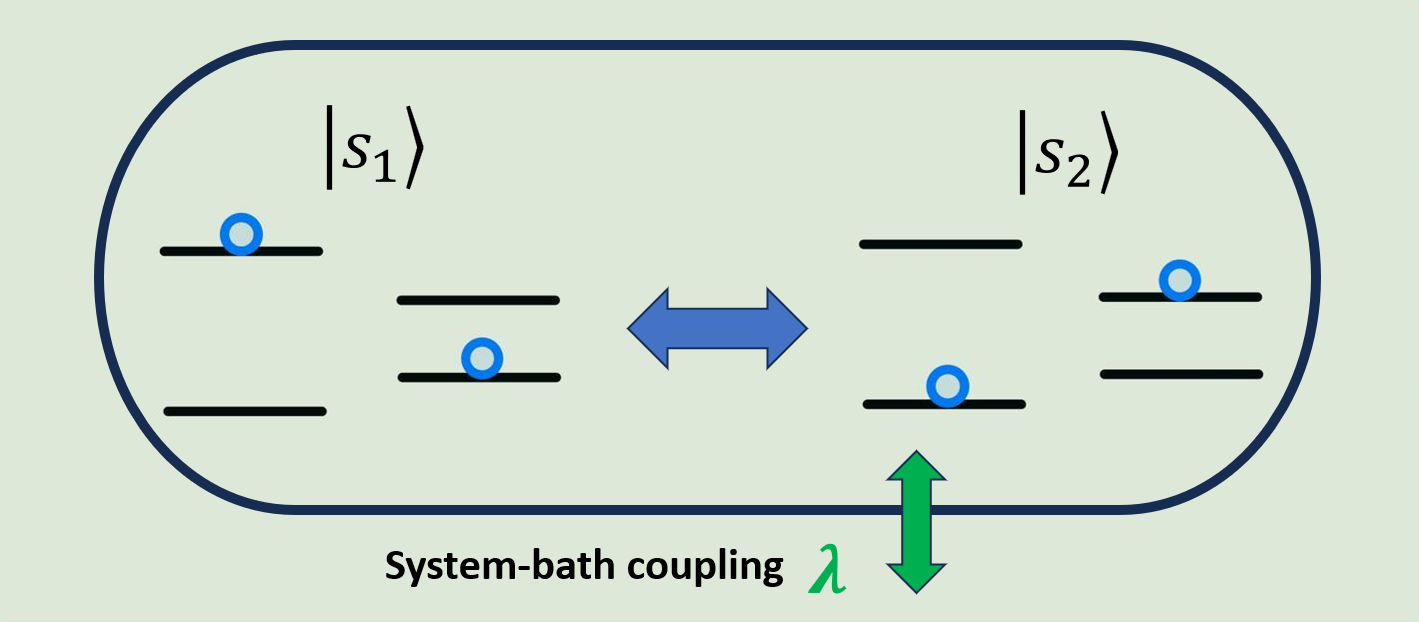
2.1. Bias Exciton Dimer System
The focus of this study lies in the investigation of the exciton dimer system, which consists of two sites, each representing a two-level system with reorganization energy , . The Hamiltonian describing this system can be expressed in second quantization form
| (1) |
where is the creation(annihilation) operator and the corresponds to coupling between and .
Notably, our research diverges from (sun2021efficient, ) upon which we have drawn inspiration. In contrast to the (sun2021efficient, ), we delve into the scenario where the two sites exhibit distinct reorganization energies ,. By encompassing this broader perspective, we aim to explore a more general case that holds relevance for the analysis of various chemically significant systems.
2.2. Open Quantum System
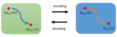
The phenomenon of interest in our study revolves around the energy transfer occurring within the exciton dimer system. This energy transfer gives rise to a Rabi-oscillation-like phenomenon, assuming no interactions with the surrounding environment. However, in most chemical processes, it is impractical and unrealistic to isolate the system from its environment. Therefore, neglecting the system-bath coupling would undermine the practicality and accuracy of our analysis. For a visual representation of our target system and its key concepts, please refer to Fig. 1, as illustrated in the article.
2.3. Hierarchical Equations of Motion(HEOM)
In classical, we adopt the HEOM method to compute the dynamics of this open quantum system. HEOM is a numerical method that adopt the Druid-Lorentz model which characterizes the system-bath coupling through the spectral density that satisfied
| (2) |
where is the reorganization energy representing the strength of the system-bath coupling, and represent the cut-up frequency correspond to the bath relaxation time scale. This model provides a framework to describe the interaction between our system and the surrounding bath.
Although HEOM method has been recognized as a highly accurate numerical method for open EET dynamics, however, it required massive layers of hierarchical truncation to solving the non-polynomial differential equations inside, which will lead to computational burden against the system size. In our work, we aim to develop computational method on quantum computer avoid using HEOM to simulate this EET dynamics.
3. Quantum Simulation Using Real Device Quantum Computer

The focus of our study will be on the excitation energy transfer(EET) between two sites in the presence of a bath. The biggest computational challenge in simulating this open quantum system on a classical computer is the computation of the system-bath coupling. To simulate this open quantum system on a quantum computer, we leverage the inherent gate noise present in today’s quantum computers. Our quantum circuit can be divided into two main parts: the dissipation part and the system propagator part. The details are provided as follows.
3.1. State Encoding
To represent the energy transfer between the two sites, we consider only two quantum state of these two sites, which are and , where former one means condition of the first site in excited state and the second site in ground state, vice versa. In our research, without loss of generality, we set the state with a larger state energy as . Notice that we neglect the states where both of the sites are in excited state or in ground state, which are relatively rare cases in EET dynamics.
To encode these two state, it’s a natural choice for us to use two qubits and set as and as . The population transfer between these two quantum states represent the energy transfer between these two sites system. With this encoding, For a quantum state produce by our two-qubit quantum circuits, neglecting the and terms, we have
| (3) |
We are able to observe the amplitude and through enough times of measurement. The and represent the population ratio of and in our EET system, shown in (b) of Fig. 1. Notice that they are also the diagonal terms of the density matrix of this two-basis quantum state. With this encoding, we are able to represent our dynamics of EET with our quantum circuit. In our research, we focus on the dynamics of , which is the population ratio of the higher energy state .
3.2. System Propagator
3.2.1. System Hamiltonian
The simulation on the quantum computer is based on the Schrödinger equation, which serves as the fundamental equation governing quantum systems. To facilitate the simulation, the Hamiltonian of the dimer system can be directly expressed in the second quantization form (let ) as
| (4) |
where the Hamiltonian is described in Eq. 1. The diagonal part of this Hamiltonian can represents the reorganization energy in each sites, and the off-diagonal terms represent the tunneling between two sites. Note that identity part in the Hamiltonian would not affect real physics, so only the bias and the tunneling matters.
In the previous work (sun2021efficient, ), Sun et al. consider a symmetric dimer system, which means energy gap of different sites are the same, and energy transfer symmetrically between them. Hence the Hamiltonian can be written in the form down below. In our work, we make extension to the cases for bias , which is a more general cases about the energy transfer between two sites with arbitrary size of energy gap. We can write it down in matrix from as
| (5) |
3.2.2. Quantum Circuits of the System Propagator
The effect of the time evolution propagator could be transform into a series of gates via a Jordan-Wigner type transformation. Due to the fact that , the time evolution operator cannot be separated into multiplication of two gate operations easily.
| (6) |
Although we are not able to separate the system propagator into multiplication of two gate operations , we are able to make good approach to it. Notice that in Eq. 6, when the is small, the second order term of t is negligible, thus it would could make approximation for , that
| (7) |
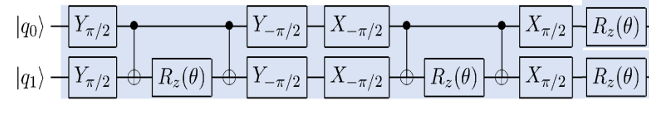
This indicates that we could implement the system propagator for a small on quantum computer through rotation X and rotation Z gates.
For a big t, by splitting time into large number of trotter steps making , we have our system propagator:
| (8) |
.
By increasing the trotter steps number , we are able approach a system propagator with a larger t on quantum circuits. A should be a reasonable choice since this kind of trotter steps maintain every split small. The quantum circuit of this system propagator are shown in (b) in Fig.2.
This approximation lead to draw back when it comes to real device implementation. When implementing this long-time propagator on a real quantum device, a deeper circuit would suffer from more gate noise. From Eq. 8, once we adopt the trotter steps , we can see that the quantum circuit depth of the propagator increase with the time . The increasing circuit depth cause the limit on the time range of our simulation when we implement the propagator on the real device quantum computer. In our research, we address this problem with transfer tensor method, which we will mention later in section 5.
3.3. Dissipative Part of the Quantum Circuit
As previously discussed, the challenging aspect of computation in this open quantum system lies in the system-bath coupling, which can be described by the Druid-Lorentz model. Notably, our primary objective is to leverage the gate errors inherent in quantum computers to simulate the dissipative aspect of energy transfer within our dimer system. This approach holds considerable merit and is worth exploring due to the nature of IBM-Q qubits. These qubits exhibit characteristics reminiscent of harmonic oscillators, thus utilizing gate noise is a good approach to mimic the dissipation observed in our dimer system. The gate noise can be understood as a result of the interaction between the qubits and their respective bath environments. By capitalizing on this intrinsic behavior, we aim to harness the natural noise present in the quantum computer to emulate the dissipative dynamics experienced by the excitons in our dimer system.
3.3.1. Dissipation Circuits
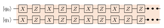
In our study, we introduce gate noises by applying identity gates . There are further discussion about the selection of this identity gate in the supplementary information. To imitate the system-bath coupling strength in HEOM, for dynamic point at time , we apply linear number of noisy identity gate before applying the system propagator , where is the frequency of this noisy identity gate. The dissipation circuits are shown in (c) in Fig. 2. A higher leads to a faster decoherence of the quantum circuits’ outcome. By adjusting the frequency , or we so call ”damping”, we are able to adjust the decoherence speed in the dynamics we generate from quantum computer, thus hopefully can simulate open quantum system with different system-bath coupling strength .
3.4. Post Processing
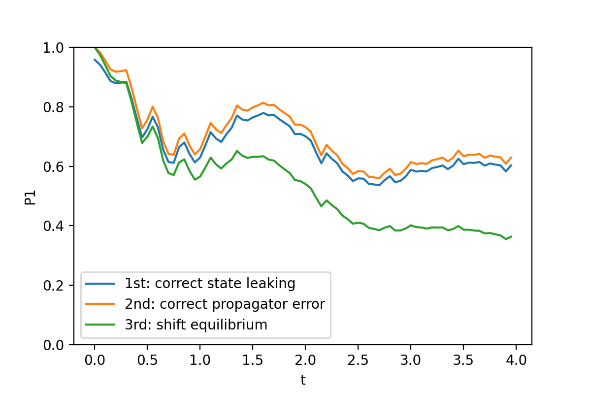
After the gate sequences of dissipative part and the system propagator part, we add measurement at the end, completing our quantum circuit. Describing the quantum state before the measurement as Eq. 3, we are able to obtain with high accuracy through enough times of rerun. Although and won’t appears through our circuits theoretically, they do appears when we run our circuits on a real quantum computer due to the noise. Here, we adjust our population by dividing all by to overcome this state leaking error. Furthermore, due to the noise caused by the system propagator, we have . Here, we fixed this with dividing all with . Last, according to Boltzmann distribution, when system reach its equilibrium, probability of staying at different state can be described as follows:
| (9) |
Here, is the state energy of , k is the Boltzmann constant and T is the temperature of this system. Since the two target states and in our system are bias, we know that and should converge to different values, and since we define as the state with a larger energy. When running our simulation on the quantum computer, We find that and from the quantum computer all converges to , meaning that through our simulation method, the temperature of our energy transfer system is equivalent to a extreme high value. To simulate a system with a finite temperature T, we can apply the following transformation
| (10) |
to fixed our dynamics. Here, is the decay constant of and for a finite temperature system. With Eq. 10, we are able to pull our simulation result to the correct equilibrium. By now, we have finished all of the post processing of .
4. Benchmark with HEOM
4.1. Linear Trotter Steps
We run our quantum circuit on IBM-Q Jakarta to test our idea. The coefficients of the Hamiltonian we are simulating on the quantum computer is , which means the Hamiltonian is
| (11) |
Here, to make distinction of the parameters from the HEOM method, we label the parameters of quantum simulation method as Q, and those parameters in HEOM method would be labeled as H.
To figure out the best range of Trotter steps, we try constant number of Trotter steps to construct our system propagator. We test our result in cases which , means we do not add noisy identity gate. We run on both the quantum simulator and the real device quantum computer, and compare with the exact result.
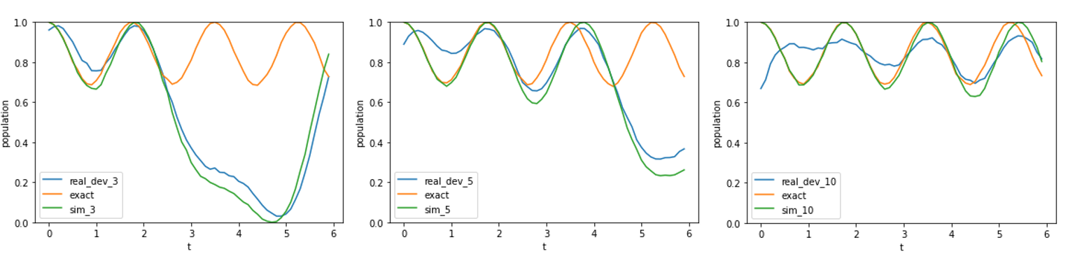
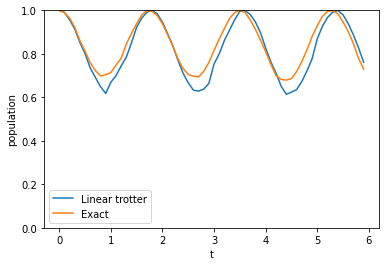
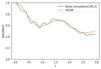
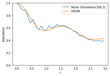
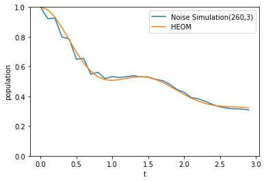
We can see from (a) in Fig. 4, the M=3 performs better in , but after , both quantum simulator and real device brokes due to the Trotter errors, meaning M=3 is not splitting into small-enough pieces. Next, we find that for (b) which is the case , real device goes very wrong both in and , while the simulator remains correct in . This indicates that for regime, the gate noise on real device is very worse thus causes the error. Errors in are caused by the Trotter error. For (c), we see the dynamics generate by the quantum simulator is relatively close to the exact dynamics, but the real device goes very bad in the regime because of increasing gate noise of the deep quantum circuits. Through this analysis, In our research, we decide to use linear trotter step to approach the system propagator. In Fig. 5, we can see that it’s a relatively good approach comparing to using constant trotter step.
4.2. Comparison with HEOM
To verify our dynamics results calculated on quantum computer, we fitted them with dynamics calculate by the HEOM method to examine whether the curves we produce by quantum computer are close to some existing system. For dynamics generated by different on quantum computer, we adjust two HEOM parameters to generate curves that fit, where is reorganization energy and is the tunnelling in the Hamiltonian of HEOM system. Rest of the system parameters, including , , system temperature , and the cut up frequency , are fixed.
From Fig. 6, we can see the fitting turns out well. The coincident of the quantum simulation dynamics and the HEOM dynamics show that our simulation method that runs on real quantum device is able to produce real physics phenomena, even after the system becomes more complicated since we consider bias .
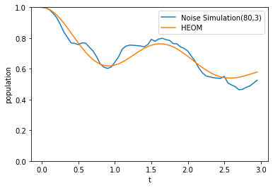
By fitting the curve produce by HEOM and our quantum simulation method, we find that for each dynamic generated by quantum simulation method, including under damping dynamics all along to the over damping dynamics, there all exist one very close dynamic generated by HEOM method, see Fig. 6. More fitting figures are shown in the supplementary information.
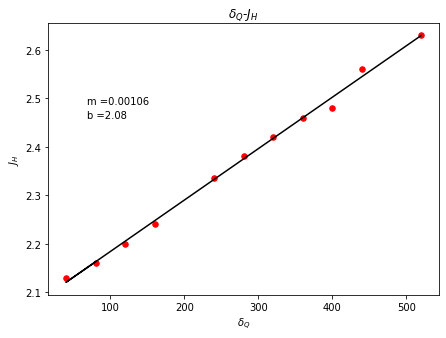
4.3. Linear Relation of the Fitting Parameters
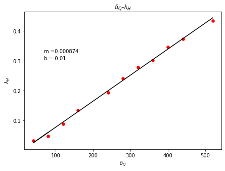
Surprisingly, when we take a look at the relation of these fitting parameters, we find the relation between and and to be very linear, see Fig. 7. In our opinion, this result is actually very surprising and non-trivial, but this seem not to only be an coincident, meaning that the intrinsic noise in the IBM-Q system do have the similar behaviour as the system-bath coupling described by the Druid-Lorentz model, which is Eq. 2. To think about it, two neighbor superconducting qubits in the IBM-Q Jakarta are also an open two-level system. It is also reasonable to think that the decoherence or the errors of the qubits is also due to the system-bath coupling in the real device quantum computer. This explains why the interpolation works. This fact provides new aspect of ways for us to model the decoherence noise inside the IBM-Q quantum computer.
4.4. Replacing the HEOM
This linear relationship give us an new idea. Although the HEOM is recognized as the high accuracy numerical method in solving this dissipative exciton dimer system, but it’s actually very costly in certain case. Due to the numerical method used in HEOM, it’s very costly to reach the same accuracy in the intermediate area compare to the the highly decoherence and coherence case.
In order to get the result in the intermediate zone without computing the HEOM method, we can make used of the linear relation shown in Fig. 7. To be more specific, we can run our quantum simulation method to fit with HEOM results with over damping and under damping condition, which is a lot more simple for HEOM method. For the intermediate part, with the linear relation of parameters shown in Fig. 7, we can obtain the we need by doing simple interpolation for imitating the result generate by HEOM. In this case, we replace the massive truncation of HEOM by our simple two-qubit circuits. This might lead to quantum advantage.
5. Long-term Dynamics Simulation through Transfer Tensor Method
Although the short-term simulation went well, we find that it’s harder for quantum computer to do long-term dynamics simulation. As the time increased, due to the increasing Trotter steps , the noise gets worse when we implementing the quantum circuits. To achieve long-term simulation of this open quantum system, we introduce the transfer tensor method(TTM). Given the fact that most propagation kernel in chemical dynamics decays fast, TTM are able to learn the propagation kernel through limited data point and make good approach on predicting the long-term dynamics.
5.1. Transfer Tensor Method
The TTM helps extend none-Markovian dynamics by generating a set of transfer tensors from a limited dynamics data. These transfer tensors combined with the original data points of the short-term dynamics, make approximate predictions for the long-term dynamics, achieving the effect of data prolongation.
The set of the dynamical maps , which , encapsulates the complete information of a quantum dynamical system (cerrillo2014non, ). For an open quantum system, if we have its density matrix for a short, equidistant time interval, where ; , we can generate dynamical maps at discrete times .
| (12) |
This set of dynamical maps provides us with ample information about this non-Markovian quantum dynamics. This allows us to derive very effective methods to learn and propagate this quantum dynamic, further reconstructing and extending our dynamics. Through the method proposed in (cerrillo2014non, ), we can compute a set of transfer tensors that satisfy
| (13) |
for . Utilizing the relationship between these transfer tensors Eq. 13 and the density matrix Eq. 12, we have
| (14) |
for . Here, we make further assumption that for an integer , satisfied that
| (15) |
This assumption holds for non-Markovian dynamics which are driven by a propagator with fast-decay the memory kernel. This means that the information between time range is enough for us to predict the subsequent data point. From the above relations, we can effectively iterate from the original data to compute the information at subsequent time points where , achieving the effect of extending the data.
5.2. Extending the Result from Quantum Computer
In our quantum simulation methods, the Trotter error and the gate noise prevents us from simulating long-duration dynamics. To solved this problem, we decided to apply TTM to extend our quantum dynamics. Using more accurate dynamics data over a short time, we generate a set of transfer tensors as described above, further extending our dynamics.
5.2.1. Generating Dynamical Map Set
In our system, the density matrix is a matrix. When expanded into a vector, we can derive a set of dynamical maps using Equation (3), where each is a matrix. To solve for the dynamical map inversely, we need four sets of density matrix series, which originate from the four initial states:
| (16) |
Without doing a full state tomography, we are not able to obtained off-diagonal terms of . To solved this problem, we approach these off-diagonal terms with the following ways. In the above discussions, the density matrix is always presented in the site basis . Through diagonalization, we can obtain the density matrix in the eigenbasis for a fixed Hamiltonian, given by
| (17) |
where the and diagonalize the system Hamiltonian. For , we made the following assumption:
| (18) |
where and , which represent the the decay constant and the angular frequency of , are derived from the fitting results of our site basis population. Combining (17) and (18), we are able to derive the off-diagonal terms of . This, in turn, allows us to solve for the dynamical maps using the aforementioned relationship (12). Once we determine the dynamical map, we can generate transfer tensors for each order. Using (Eq. 15), we can then extend our dynamics.
6. Validity of Transfer Tensor Method
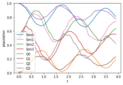
We test the TTM method on the results produce by a quantum simulator and a real quantum device IBMQ Jakarta. To apply TTM method, it requires 4 dynamics starting from 4 independent initial states, which is described in (16). Without doing full state tomography, we are only able to obtain the population and of each site, which is the diagonal terms of density matrix . From the measurement result of quantum computer, we applied (17) and (18) to get the off-diagonal terms of the density matrices.
6.1. Quantum Simulator
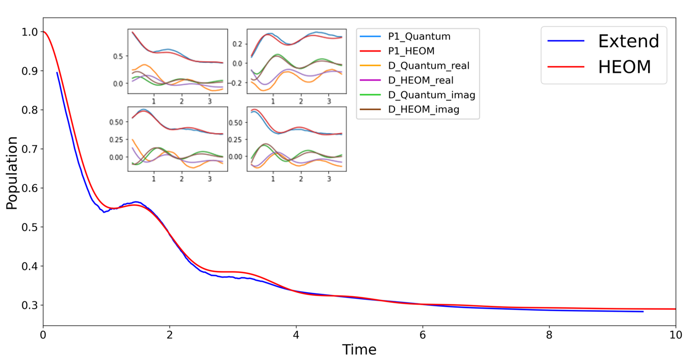
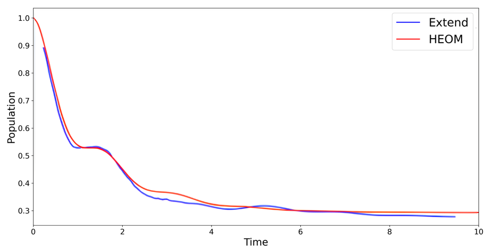
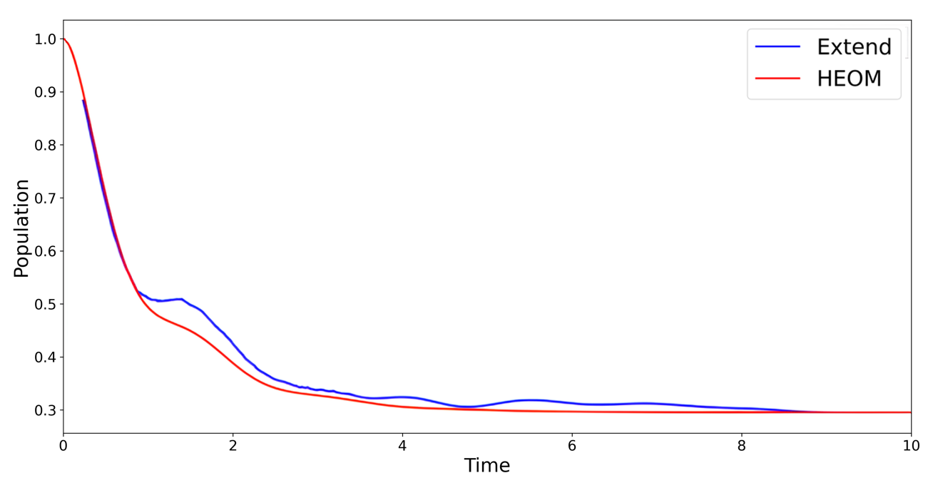
From the result of the qiskit simulator, we extend dynamics of starting at initial state for , depolarizing error rate = 0.002. In (a) in Fig. 8, we provide comparison of density matrix between simulator and HEOM dynamics starting from four initial state, for . In (b), we see the extension of the dynamics from simulator fits very well with the HEOM dynamics for , which is almost 3 times of original training data.
6.2. Real Device
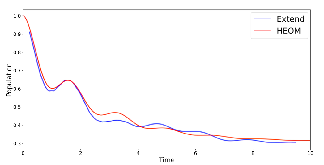
Although the extended results on Qiskit’s quantum simulator fit the HEOM results well, we find it very hard to reproduce on real-device quantum computer, due to the two chaotic dynamics which starts from and on a real device when . Unlike those dynamics starting from , these two dynamics don’t seem to fit the results of HEOM method. It is expected since these two initial states are superposition state of and , which needs the quantum device to be less noisy to perform well. In all cases, we find the dynamics from all four initial states fit the HEOM better only for the case , which represents dynamics of the energy transfer with no system-bath coupling.
Here, we try to apply TTM as an error mitigation method. We compare these following three dynamics:
-
•
dynamics extended to generated by TTM with real device result from ,
-
•
real device dynamics from ,
-
•
HEOM dynamics from .
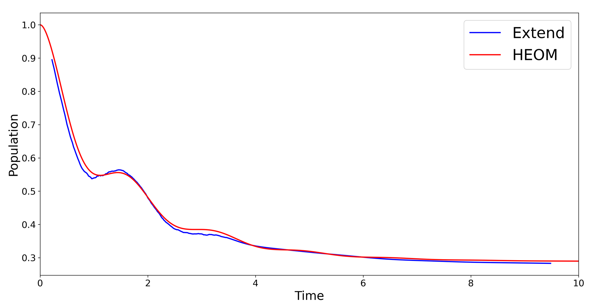
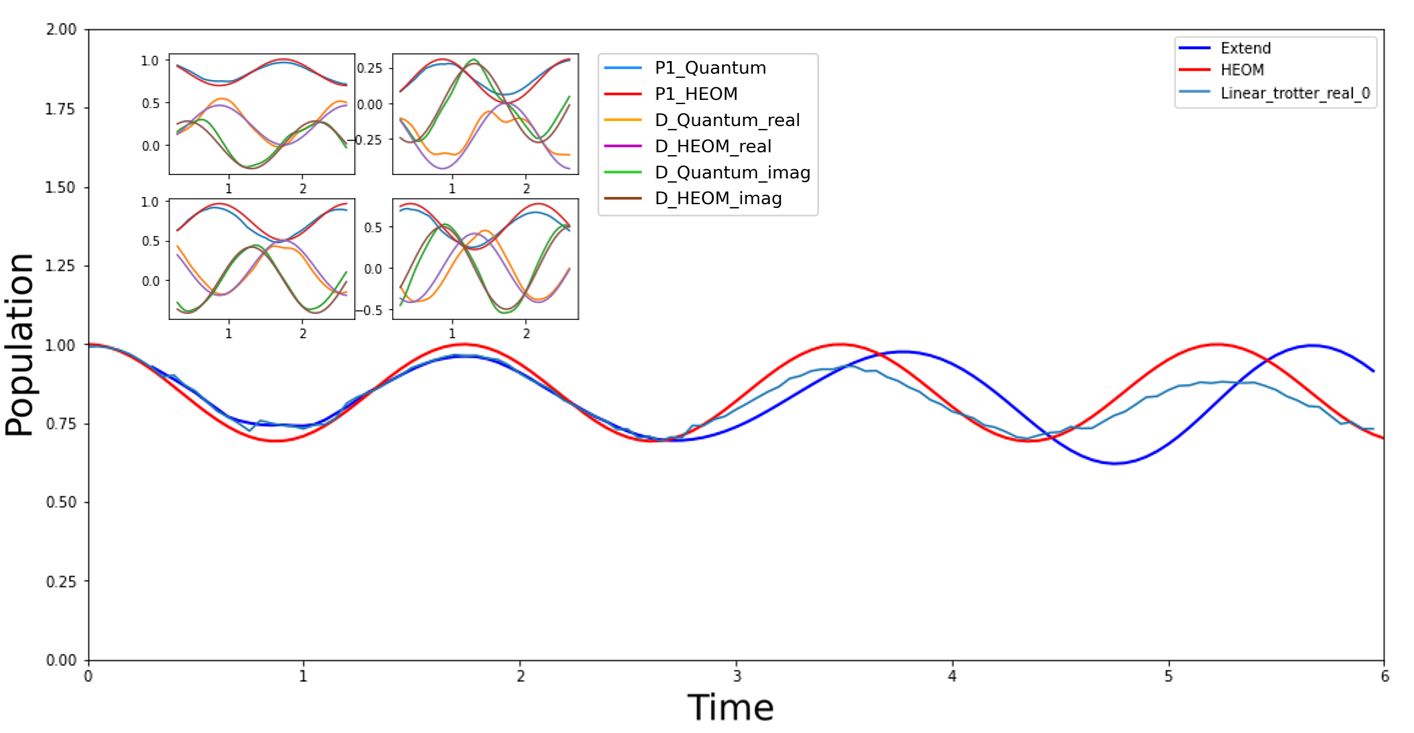
By applying TTM on the the data points from , which is about the first wave of the dynamics, we extend our dynamics to , see Fig. 11. We can see, comparing to the real device dynamics which decoherent as the times grow, the extended dynamics produce by TTM actually preserve the amplitude, since we use the previous part of the dynamics as our learning data point. But as we can see, although the dynamics including the off-diagonal terms of are very close to the exact dynamics produced by HEOM method, we still fail to reproduce the right frequency of this energy transfer dynamics due to the limited range of the learning data points. In this case, although the TTM-extended dynamics are still not able to outperform the dynamics produced by real device quantum computers, we showed the potential of applying this TTM method to extend dynamics simulations.
7. Concluding Remarks
In this NISQ era, it’s very hard for any algorithm to implement on the real quantum computer due to the terrible amount of errors when performing quantum operations. In this work, we successfully simulate the energy transformation between two bias sites in a dissipative environment via IBM-Q Jakarta, using only 2 qubits.
Also, We show the intrinsic noise some how performs similar to the effective reorganization energy between system and the bath described in Druid-Lorentz modelEq. 2. The linear relation between identity gate frequency and corresponding allows us to find the correct through interpolation and successfully predict this open quantum system with the real device quantum computer without applying the HEOM method in the intermediate regime of system-bath coupling, leading us toward quantum advantage.
To deal with the increasing errors cause by Trotter expansion when performing the system propagator, we adopt transfer tensor method to extend our short dynamics. On the theory sides, we provide an accurate way to infer the off-diagonal terms of a density matrix from an observed site 1 population . Through this way, we are able to construct the dynamical maps s without doing quantum state tomography with the quantum circuits, further accomplished the transfer tensor method. For the experiments, we are able to extend the dynamics simulated by quantum simulator into 3 times longer. On the real-device, the TTM-extended result failed to outperform the dynamics produced directly by quantum computer due to limited range of the learning period and the fluctuation during the dynamics, but we still see it preserved the amplitude better than the quantum computer. Through the experiment on extending dynamics produced by the simulator, we demonstrate the potential of applying TTM as a error mitigation method in the near future.
References
- [1] Shin Sun, Li-Chai Shih, and Yuan-Chung Cheng. Efficient quantum simulation of open quantum system dynamics on noisy quantum computers, 2021.
- [2] Javier Cerrillo and Jianshu Cao. Non-markovian dynamical maps: numerical processing of open quantum trajectories. Physical review letters, 112(11):110401, 2014.
- [3] Michael A Nielsen and Isaac L Chuang. Quantum computation and quantum information. Phys. Today, 54(2):60, 2001.
- [4] Dave Bacon, Andrew M Childs, Isaac L Chuang, Julia Kempe, Debbie W Leung, and Xinlan Zhou. Universal simulation of markovian quantum dynamics. Physical Review A, 64(6):062302, 2001.
- [5] Iulia M Georgescu, Sahel Ashhab, and Franco Nori. Quantum simulation. Reviews of Modern Physics, 86(1):153, 2014.
- [6] Ehud Altman, Kenneth R Brown, Giuseppe Carleo, Lincoln D Carr, Eugene Demler, Cheng Chin, Brian DeMarco, Sophia E Economou, Mark A Eriksson, Kai-Mei C Fu, et al. Quantum simulators: Architectures and opportunities. PRX Quantum, 2(1):017003, 2021.
- [7] Man-Hong Yung, James D Whitfield, Sergio Boixo, David G Tempel, and Alán Aspuru-Guzik. Introduction to quantum algorithms for physics and chemistry. Quantum Information and Computation for Chemistry, pages 67–106, 2014.
- [8] Peter JJ O’Malley, Ryan Babbush, Ian D Kivlichan, Jonathan Romero, Jarrod R McClean, Rami Barends, Julian Kelly, Pedram Roushan, Andrew Tranter, Nan Ding, et al. Scalable quantum simulation of molecular energies. Physical Review X, 6(3):031007, 2016.
- [9] James I Colless, Vinay V Ramasesh, Dar Dahlen, Machiel S Blok, Mollie E Kimchi-Schwartz, Jarrod R McClean, Jonathan Carter, Wibe A de Jong, and Irfan Siddiqi. Computation of molecular spectra on a quantum processor with an error-resilient algorithm. Physical Review X, 8(1):011021, 2018.
- [10] Yudong Cao, Jonathan Romero, Jonathan P Olson, Matthias Degroote, Peter D Johnson, Mária Kieferová, Ian D Kivlichan, Tim Menke, Borja Peropadre, Nicolas PD Sawaya, et al. Quantum chemistry in the age of quantum computing. Chemical reviews, 119(19):10856–10915, 2019.
- [11] Sam McArdle, Suguru Endo, Alán Aspuru-Guzik, Simon C Benjamin, and Xiao Yuan. Quantum computational chemistry. Reviews of Modern Physics, 92(1):015003, 2020.
- [12] John Preskill. Quantum computing in the nisq era and beyond. Quantum, 2:79, 2018.
- [13] Prakash Murali, Jonathan M Baker, Ali Javadi-Abhari, Frederic T Chong, and Margaret Martonosi. Noise-adaptive compiler mappings for noisy intermediate-scale quantum computers. In Proceedings of the twenty-fourth international conference on architectural support for programming languages and operating systems, pages 1015–1029, 2019.
- [14] Emanuel Knill, Raymond Laflamme, and Wojciech H Zurek. Resilient quantum computation. Science, 279(5349):342–345, 1998.
- [15] Sergey Bravyi, Matthias Englbrecht, Robert König, and Nolan Peard. Correcting coherent errors with surface codes. npj Quantum Information, 4(1):55, 2018.
- [16] Heinz-Peter Breuer and Francesco Petruccione. The theory of open quantum systems. Oxford University Press, USA, 2002.
- [17] Ulrich Weiss. Quantum dissipative systems. World Scientific, 2012.
- [18] Roberta Croce and Herbert van Amerongen. Light harvesting in oxygenic photosynthesis: Structural biology meets spectroscopy. Science, 369(6506):eaay2058, 2020.
- [19] Eric A Arsenault, Yusuke Yoneda, Masakazu Iwai, Krishna K Niyogi, and Graham R Fleming. Vibronic mixing enables ultrafast energy flow in light-harvesting complex ii. Nature communications, 11(1):1460, 2020.
- [20] Lili Wang, Marco A Allodi, and Gregory S Engel. Quantum coherences reveal excited-state dynamics in biophysical systems. Nature Reviews Chemistry, 3(8):477–490, 2019.
- [21] Shahnawaz Rafiq and Gregory D Scholes. From fundamental theories to quantum coherences in electron transfer. Journal of the American Chemical Society, 141(2):708–722, 2018.
- [22] Tae Wu Kim, Sunhong Jun, Yoonhoo Ha, Rajesh K Yadav, Abhishek Kumar, Chung-Yul Yoo, Inhwan Oh, Hyung-Kyu Lim, Jae Won Shin, Ryong Ryoo, et al. Ultrafast charge transfer coupled with lattice phonons in two-dimensional covalent organic frameworks. Nature Communications, 10(1):1873, 2019.
- [23] Wojciech Hubert Zurek. Decoherence, einselection, and the quantum origins of the classical. Reviews of modern physics, 75(3):715, 2003.
- [24] Yoshitaka Tanimura and Ryogo Kubo. Time evolution of a quantum system in contact with a nearly gaussian-markoffian noise bath. Journal of the Physical Society of Japan, 58(1):101–114, 1989.
- [25] Yoshitaka Tanimura. Stochastic liouville, langevin, fokker–planck, and master equation approaches to quantum dissipative systems. Journal of the Physical Society of Japan, 75(8):082001, 2006.
- [26] Akihito Ishizaki and Graham R Fleming. Unified treatment of quantum coherent and incoherent hopping dynamics in electronic energy transfer: Reduced hierarchy equation approach. The Journal of chemical physics, 130(23), 2009.
- [27] Jinshuang Jin, Xiao Zheng, and YiJing Yan. Exact dynamics of dissipative electronic systems and quantum transport: Hierarchical equations of motion approach. The Journal of chemical physics, 128(23), 2008.
- [28] Sabrina Maniscalco, Jyrki Piilo, F Intravaia, F Petruccione, and A Messina. Simulating quantum brownian motion with single trapped ions. Physical Review A, 69(5):052101, 2004.
- [29] Andrea Chiuri, Chiara Greganti, Laura Mazzola, Mauro Paternostro, and Paolo Mataloni. Linear optics simulation of quantum non-markovian dynamics. Scientific reports, 2(1):968, 2012.
- [30] Sarah Mostame, Patrick Rebentrost, Alexander Eisfeld, Andrew J Kerman, Dimitris I Tsomokos, and Alán Aspuru-Guzik. Quantum simulator of an open quantum system using superconducting qubits: exciton transport in photosynthetic complexes. New Journal of Physics, 14(10):105013, 2012.
- [31] P Anton et al. Studying light-harvesting models with superconducting circuits nat, 2018.
- [32] Bi-Xue Wang, Ming-Jie Tao, Qing Ai, Tao Xin, Neill Lambert, Dong Ruan, Yuan-Chung Cheng, Franco Nori, Fu-Guo Deng, and Gui-Lu Long. Efficient quantum simulation of photosynthetic light harvesting. NPJ Quantum Information, 4(1):52, 2018.
- [33] Nils Trautmann and Philipp Hauke. Trapped-ion quantum simulation of excitation transport: Disordered, noisy, and long-range connected quantum networks. Physical Review A, 97(2):023606, 2018.
- [34] Richard P Feynman et al. Simulating physics with computers. Int. j. Theor. phys, 21(6/7), 2018.
- [35] Seth Lloyd. Universal quantum simulators. Science, 273(5278):1073–1078, 1996.
- [36] Christine Maier, Tiff Brydges, Petar Jurcevic, Nils Trautmann, Cornelius Hempel, Ben P Lanyon, Philipp Hauke, Rainer Blatt, and Christian F Roos. Environment-assisted quantum transport in a 10-qubit network. Physical review letters, 122(5):050501, 2019.
- [37] Hong-Yi Su and Ying Li. Quantum algorithm for the simulation of open-system dynamics and thermalization. Physical Review A, 101(1):012328, 2020.
- [38] Guillermo García-Pérez, Matteo AC Rossi, and Sabrina Maniscalco. Ibm q experience as a versatile experimental testbed for simulating open quantum systems. npj Quantum Information, 6(1):1, 2020.
- [39] Brian Rost, Barbara Jones, Mariya Vyushkova, Aaila Ali, Charlotte Cullip, Alexander Vyushkov, and Jarek Nabrzyski. Simulation of thermal relaxation in spin chemistry systems on a quantum computer using inherent qubit decoherence. arXiv preprint arXiv:2001.00794, 2020.
8. Supplementary Information
8.1. Identity Gate Error
To incorporate IBM-Q computer errors into our simulation, we examined their nature. The original study revealed that these errors are not random Gaussian noise (depolarizing errors). If they were, applying numerous gates on a single qubit would only result in depolarization errors, causing the Bloch vector to shrink towards the center without rotation. However, the experiment demonstrated significant rotation of the gate, indicating the presence of non-depolarizing errors. This finding is important as it affects the preservation of accurate information. Intrigued by these results, we replicated the experiment on the IBM-Q computer ”Jakarta” to further investigate these errors.
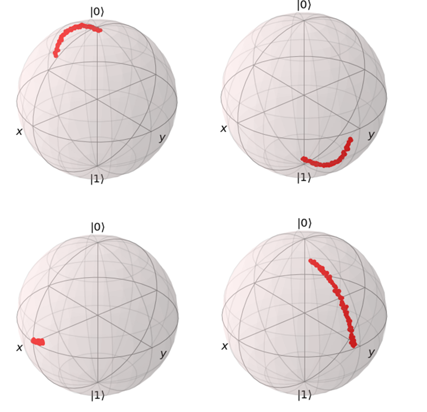
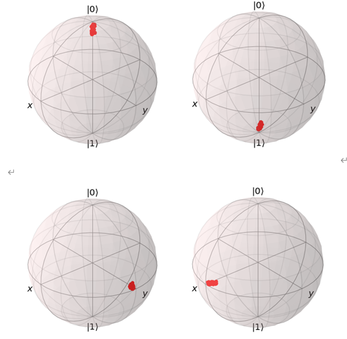
We can canceled the shifting error and produce pure depolarization noises by adding Z gates to reflect the over rotation in order to cancel out the rotation error from the X gates, shown above.
According to Fig. 13, by applying numerous gate, we’re able to prepare artificial coherence, which we used in our research to simulate open quantum system.