When accurate prediction models yield harmful self-fulfilling prophecies

Abstract

Objective Prediction models are popular in medical research and practice. By predicting an outcome of interest for specific patients, these models may help inform difficult treatment decisions, and are often hailed as the poster children for personalized, data-driven healthcare. Many prediction models are deployed for decision support based on their prediction accuracy in validation studies. We investigate whether this is a safe and valid approach.

Materials and Methods We show that using prediction models for decision making can lead to harmful decisions, even when the predictions exhibit good discrimination after deployment. These models are harmful self-fulfilling prophecies: their deployment harms a group of patients but the worse outcome of these patients does not invalidate the predictive power of the model.

Results Our main result is a formal characterization of a set of such prediction models. Next we show that models that are well calibrated before and after deployment are useless for decision making as they made no change in the data distribution.

Discussion Our results point to the need to revise standard practices for validation, deployment and evaluation of prediction models that are used in medical decisions.

Conclusion Outcome prediction models can yield harmful self-fulfilling prophecies when used for decision making, a new perspective on prediction model development, deployment and monitoring is needed.

Word count: 3516

1 Introduction

Clinicians and medical researchers frequently employ outcome prediction models (OPMs): statistical models that predict a certain medical outcome based on a patient’s characteristics [1]. Researchers develop OPMs to provide information to clinicians so they may use this information in difficult treatment decisions (e.g. [2]). In some cases, clinicians will treat patients with a bad expected outcome more aggressively, for example by giving cholesterol lowering medication to patients with a high predicted risk of a heart attack [3, 4]. In other cases, for instance when the treatment is burdensome or scarcely available (e.g. ventilator machines on the intensive care during a pandemic), clinicians may reserve treatment for patients with a good predicted outcome.

Many such OPMs are added to the protocol of care by designing specific thresholds for specific actions [3]. If the predicted outcome is above or below the threshold a certain action is taken, e.g. the patient receives a more aggressive therapy. The basis for including an OPM in a care protocol is generally predictive accuracy in validation studies [5]. In these validation studies, the OPM may or may not have been used to inform treatment decisions.

At first, it may seem that this approach is beneficial since giving more information should lead to better treatment decisions. However, implementing a prediction model for treatment decisions is an intervention that changes treatment decisions and thus patient outcomes. Whether this change in treatment policy improves patient outcomes is not determined by prediction accuracy in a validation study [6]. For instance, in cases where a certain patient subpopulation historically received suboptimal care, an accurate OPM will predict a worse outcome for these patients compared to similar patients outside of the subpopulation. If clinicians decide to withhold effective treatments (e.g., due to scarcity or perceived futility) to this underserved subpopulation based on the OPM’s prediction of a bad outcome, the implementation of the OPM perpetuated biases or caused harm to these patients, despite its accuracy. Moreover, the implementation of this harmful new policy brought about the scenario predicted by the OPM, as in a self-fulfilling prophecy. One concrete example where clinicians treat patients with a bad expected outcome less aggressively is in small cell lung cancer. Prognostic scores for small cell lung cancer patients, such as the Manchester score developed in [7] are specifically intended to not over-treat patients with a bad predicted outcome because this is expected to be futile [8, 9].

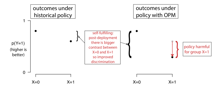
Figure 1: Some outcome prediction models yield harmful self-fulfilling prophecies when used to guide treatment decisions, meaning the new policy harms a subgroup of patients but the prediction model has good discrimination post-deployment.

In this article we address the following questions: 1) Under what conditions is a new policy based on an OPM going to be harmful, meaning that it leads to worse outcomes than before using the model? 2) In what circumstances would such a harmful policy go undetected by measures of discrimination or calibration? In what follows we provide a formalization of the case where patients with a high predicted probability of the outcome get treatment, where the outcome may be be preferable (e.g. 1-year survival) or undesirable (e.g. a heart attack). Specifically, we examine the setting where a new OPM is supposed to ‘personalize’ an existing treatment policy by considering additional features. Section 2 provides notation and definitions, Section 3 presents the main results concerning OPMs that are harmful and self-fulfilling prophecies. We first show that even in a simple setup with a binary covariate, a non-trivial subset of OPMs yields harmful self-fulfilling prophecies. This means that such models cause harm but exhibit good discrimination on post-deployment data, meaning that naively interpreting this as a successful deployment leads to harmful policies. Next, perhaps surprisingly, we show that when an OPM is well calibrated on both 1) the historical data and 2) a validation study where the model is used for treatment decisions, the OPM is not useful for decision making.

Based on our results, several common practices in building and deploying OPMs intended for decision making need revision: 1. Developing OPMs on observational data without regard of the historical treatment policy is potentially dangerous, because the change in treatment policy between pre- and post-deployment is what determines the effect of the model on patient outcomes. 2. Implementing a personalized outcome prediction model is not always beneficial, even if the model is very accurate. 3. When monitoring discrimination prospectively after deployment, sometimes good discrimination means a harmful model and sometimes a beneficial one.

2 Notation and definitions

We assume a binary treatment $T$, a binary outcome $Y$ and a binary feature $X\in\mathcal{X}=\{0,1\}$. We denote the outcome obtained with setting treatment $T$ to $t$ as $Y_{t}$. An OPM is a function trained on historical data to predict the outcome of interest. We use $\pi_{i}(X)$ to denote a policy for assigning treatment, possibly conditional on $X$, with an index $i$ to indicate what policy we are referring to. Throughout the paper $\pi_{0}$ will be used to indicate the historic treatment policy that was in place in the data in which the OPM was developed.

We assume the historical policy is constant and deterministic, meaning that it is always equal to 0 or 1 (i.e. patients were always treated or never treated). Next we define what it means to craft a policy based on an existing OPM. We will be concerned only with threshold-based policies, namely policies that assign treatment based on a threshold $\lambda\in\mathbb{R}$. In our setup, policies assign treatment to patients only if the expected outcome is above $\lambda$, which could mean either a desirable outcome (e.g. 1-year survival) or undesirable (e.g. a heart attack).

Definition 2.1 (Policy informed by OPM).

Let $f:X\to[0,1]$ be an OPM and $\lambda\in\mathbb{R}$ a threshold. We call $\pi_{f}$ a policy informed by $f$ and define it as follows

$$\pi_{f}(x)=\begin{cases}1\hskip 28.45274ptf(x)>\lambda\\ 0\hskip 28.45274ptf(x)\leq\lambda\end{cases}$$ (1)

Such policies describe the post-deployment scenario, when the OPM influences treatment assignment. This deployment will change some of the (conditional) probability distributions compared to pre-deployment. We distinguish probabilities pre- and post-implementation using subscripts: $p_{i}(.)$ with $i\in\{0,f\}$ respectively. We now present the first key idea of this paper, namely the special class of OPMs whose predictions are realized upon implementation. We consider as a metric of discrimination the popular ‘Area under the ROC-curve’ (AUC [10]).

Definition 2.2 (Self-fulfilling OPM).

Let $f:X\to[0,1]$ be an OPM, $\lambda\in\mathbb{R}$ a threshold and let $\pi_{f}$ be the policy informed by $f$. Let $AUC(\pi_{i})$ denote the AUC of this OPM on data generated with the historic policy ($\pi_{0}$) or with the policy defined by $f$ ($\pi_{f}$). We call the pair $(f,\lambda)$ self-fulfilling if the AUC remains the same or increases post-deployment, namely iff:

$$\text{AUC}(\pi_{f})\geq\text{AUC}(\pi_{0})$$ (2)

Finally, we specify what we mean with an OPM being harmful in comparison with the status quo.

Definition 2.3 (Harmful OPM).

Let $f:X\to[0,1]$ be an OPM, $\lambda\in\mathbb{R}$ a threshold, let $\pi_{0}$ denote the historic treatment policy and let $\pi_{f}$ be the policy informed by $f$. We write the expected outcomes under the different policies as

$$p_{i}(Y=1|X)=\operatorname{\mathbb{E}}_{T\sim\pi_{i}(X)}p(Y_{T}=1|X)$$ (3)

where $i=0$ denotes the historical distribution and $i=f$ the distribution under $\pi_{f}$. We call $f$ harmful for the group with $X=x$ with $p(X=x)>0$ if the expected outcome of the group is worse under the new policy compared to the old policy, namely when $Y=1$ is preferable iff

$$p_{f}(Y=1|X=x)<p_{0}(Y=1|X=x)$$ (4)

or when $Y=0$ is preferable iff

$$p_{f}(Y=1|X=x)>p_{0}(Y=1|X=x)$$ (5)

When a policy informed by an OPM is both harmful and self-fulfilling we have a worst-case scenario where the new policy is causing harm to a subgroup but this, perhaps counter-intuitively, does not result in a decrease in AUC post-deployment.

3 Results

We now move to the main results, whose proofs can be found in Appendix B. The setting where a new OPM is supposed to ‘personalize’ an already existing treatment policy by considering more features is encoded as follows: the new OPM considers a feature $X$ that was previously ignored by the historical policy, specifically $\pi_{0}$ is constant and deterministic. In addition, the new policy $\pi_{f}$ is not constant but varies with $X$.

3.1 Harmful models may have good discrimination post-deployment

We state our main observation as an informal theorem.

Theorem 3.1 (Informal main result).

Let $\pi_{f}$ be the policy informed by the OPM $f$ using a threshold $\lambda$. Assume that: i) the historical policy $\pi_{0}$ is constant and deterministic ii) the new policy $\pi_{f}$ is not constant, i.e. not always equal to 1 or 0 and iii) the marginal distribution of $X$ is the same pre and post deployment: $p_{i}(X)=p(X)$ for $i\in\{0,f\}$.

Under these assumptions, a non-trivial subset of OPMs will demonstrate good post-deployment discrimination because they yield self-fulfilling prophecies, and at the same time their deployment harmed patients.

The theorem is exemplified by Figure 1. We proceed to characterize the contours of the subset of self-fulfilling and harmful OPMs.

Proposition 3.2 (Self-fulfilling).

Suppose the assumptions of Theorem 3.1 hold. Furthermore assume that the joint probabilities of $X$ and $Y$ are non-deterministic both pre- and post-deployment:

$$0<p_{i}(Y=1,X=x)<1,\forall x\in\mathcal{X}$$ (6)

Then the following two statements are true: i) if the treatment effect is always positive, namely $\forall x\in\mathcal{X}:p(Y_{1}=1|X=x)\geq p(Y_{0}=1|X=x)$, then $(f,\lambda)$ is self-fulfilling; ii) if the treatment effect is always negative, meaning $\forall x\in\mathcal{X}:p(Y_{1}=1|X=x)<p(Y_{0}=1|X=x)$, then $(f,\lambda)$ is not self-fulfilling.

Remark 3.3.

Proposition 3.2 gives sufficient conditions for an OPM yielding a self-fulfilling prophecy. When $Y=1$ is preferable, meaning the new policy treats only those with a favorable predicted outcome (e.g. under resource scarcity), this happens when the treatment effect is beneficial for all values of $X$. When instead $Y=0$ is preferable, meaning the ‘treat high-risk patients’-setting, the sufficient condition is that treatment is detrimental for all values of $X$. Treatments that are always detrimental are less likely to be used in practice as most often treatments are approved for use after they are proven to be beneficial on average with an RCT. In this case of ‘treat high risk’, self-fulfilling prophecies may still occur when the treatment is detrimental to a subgroup of patients.

Remark 3.4.

Proposition 3.2 does not depend on the OPM’s discrimination in the historical data, meaning that models with ‘good’ discrimination (i.e. high AUC) and ‘bad’ discrimination (low AUC) are equally susceptible to yielding self-fulfilling prophecies under the conditions of the proposition.

Now we know when OPMs are self-fulfilling and thus have good post-deployment discrimination, but can these self-fulfilling OPMs also be harmful? Proposition 3.5 indicates that they can:

Proposition 3.5 (Harmful).

Under the assumptions of Theorem 3.1, when $Y=1$ is preferable, $f$ is harmful for the group with $X=x$ iff

1. $\pi_{0}(x)=1$ and $\pi_{f}(x)=0$ and $p(Y_{1}=1|X=x)>p(Y_{0}=1|X=x)$ or

2. $\pi_{0}(x)=0$ and $\pi_{f}(x)=1$ and $p(Y_{1}=1|X=x)<p(Y_{0}=1|X=x)$

When $Y=0$ is preferable, the inequality signs reverse.

The conditions of this Proposition indicate that, as one would expect, removing the treatment from this group is harmful iff $p(Y_{1}=1|X=x)>p(Y_{0}=1|X=x)$ (assuming $Y=1$ is preferable), i.e. if the effect of the treatment was positive for this group. Conversely, adding treatment to group with $X=x$ is damaging iff $p(Y_{1}=1|X=x)<p(Y_{0}=1|X=x)$ (when $Y=1$ is preferable), meaning that the treatment decreases the outcome for the group.

Remark 3.6 (harmful OPMs are marginally harmful).

Under the assumptions of Theorem 3.1, OPMs that are harmful for one subgroup are also harmful on average, as the other subgroup’s treatment policy and outcomes do not change.

Taking together Proposition 3.2 on when OPMs yield self-fulfilling prophecies and Proposition 3.5 on when OPM deployment is harmful, we reach the perhaps surprising conclusion of Theorem 3.1: even in the simple setup of binary treatment and binary $X$, some OPMs are both self-fulfilling prophecies, and thus demonstrate good post-deployment discrimination, and harm a patient subgroup when deployed. We present an example based on realistic medical assumptions in Appendix A. In Table 1 we list the cases in which OPM deployment is harmful, based on three pieces of information that are available post-deployment: i) is $Y=1$ preferable or undesirable? ii) was the historical policy ‘treat everyone’ or ‘treat no one’? and iii) did the AUC of the OPM increase post-deployment compared to the AUC pre-deployment (i.e. is the OPM self-fulfilling)? Finally, we note that the performance of the OPM on the historical data does not feature in the assumptions or statement of Proposition 3.5. This entails, contrary to what some may expect, that a high performance on historical data, including external validation, provides no guarantee on whether the OPM-driven policy will be beneficial.

interpretation of $Y=1$ (and policy)	$\pi_{0}$	$AUC(\pi_{f})-AUC(\pi_{0})$	OPM deployment was
	0 (treat no one)	>0 (self-fulfilling)	harmful
	0 (treat no one)	<0 (not self-fulfilling)	beneficial
undesirable (treat high risk patients)	1 (treat everyone)	>0 (self-fulfilling)	beneficial
	1 (treat everyone)	<0 (not self-fulfilling)	harmful
	0 (treat no one)	>0 (self-fulfilling)	beneficial
	0 (treat no one)	<0 (not self-fulfilling)	harmful
desirable (treat low risk patients)	1 (treat everyone)	>0 (self-fulfilling)	harmful
	1 (treat everyone)	<0 (not self-fulfilling)	beneficial

Table 1: Overview of when OPM deployment was harmful, based on three pieces of information that are available post-deployment. This table excludes the trivial case where nothing changes post-deployment (see Theorem 3.8). $\pi_{0}$: historical treatment policy (either treat everyone or treat no one in our setup); $AUC(\pi_{f})$: AUC in distribution post deployment; $AUC(\pi_{0})$: AUC in distribution pre deployment; OPM: outcome prediction model

3.2 OPMs that are calibrated pre- and post-deployment are not useful for treatment decisions

Monitoring discrimination post-deployment and naively interpreting good post-deployment discrimination as a safe deployment is thus not a good strategy, as self-fulfilling prophecies have good post-deployment discrimination but can still be harmful depending on the context. We now turn to another key metric of OPMs predicting the risk of an outcome: calibration [11, 12, 13] and investigate how post-deployment calibration relates to harmful policies. We use the following definition of calibration:

Definition 3.7.

Let $p(X,Y)$ be a joint distribution over feature $X$ and binary outcome $Y$, and $f:X\to[0,1]$ an OPM. $f$ is calibrated with respect to $p(X,Y)$ if, for all $\alpha\in[0,1]$ in the range of $f$, $\operatorname{\mathbb{E}}_{X,Y\sim p(X,Y)}[Y|f(X)=\alpha]=\alpha$.

We distinguish two distributions $p_{i}(Y=1|X)$ on which an OPM can be calibrated depending on the treatment policy indicated with $i\in\{0,f\}$. Theorem 3.1 states that harmful OPMs can have good pre- and post-deployment discrimination, but can they also have good calibration? The following theorem shows that OPMs that are calibrated pre- and post-deployment do not lead to better treatment decisions.

Theorem 3.8.

Let $f$ be an OPM that is calibrated on historical data and $\pi_{f}$ be non constant. Such OPM is calibrated on the deployment distribution iff for every $x\in\mathcal{X}$:

$$\pi_{0}(x)=\pi_{f}(x)\text{ \emph{or} }p(Y_{1}=1|X=x)=p(Y_{0}=1|X=x)$$ (7)

Note that this entails that for all $x\in\mathcal{X}$ either the treatment policy does not change, or it changes where it is irrelevant because for that value of $X$ the treatment effect is zero. Both cases imply the implementation of the OPM is inconsequential. This may seem counterintuitive, but an OPM being calibrated both before and after deployment means the distribution has not changed, so the policy remains the same or the policy was changed where it is irrelevant (i.e. no treatment effect). So an OPM that is calibrated on the development cohort, which remains calibrated post deployment is not a useful OPM.

4 Related work

Previous work noted that prediction accuracy does not equal value for treatment decision making [14, 15, 6]. Here we exactly characterize a set of prediction models that yield harmful self-fulfilling prophecies. The idea that model deployment changes the distribution and affects model performance was noted in several lines of previous work. Several authors noted that model performance may degrade over time due to the effect of deployment of the model [16, 17], but we study the case where model performance does not degrade but the implementation of it still caused harm. In fact, degraded discrimination may indicate benefit of the deployment. [18] and [19] study the setting of performing successive model updates, each time after deploying the previous model for decision making. [18] study when over successive deployments predictive performance stabilizes or reaches optimality, and [19] study both model stability and the effect of model deployment on outcomes. Our work may be seen as a special case of these works with only a single model deployment and no model update, but we add new insights as we describe exactly when a single model deployment leads to harm and good post-deployment discrimination. Several groups have studied out-of-distribution generalization and its connections to causality and invariance [20, 21, 22] with the aim of removing a model’s dependency on spurious correlations. Again our work differs as we are interested in characterizing model performance following a very specific distribution change (a treatment policy change induced by a prediction model) that is particularly relevant in health care, and our main concern is the effect of this policy change on outcomes. Finally, current guidelines on prediction model validation and deployment focus on discrimination and calibration only, not on these newer invariance metrics [15, 5].

5 Discussion

We showed how OPMs can be harmful self-fulfilling prophecies, meaning they lead to patient harm when used for treatment decision making, but retain good discrimination after deployment. Moreover, we showed that when a model is well calibrated before and after deployment it is not useful for treatment decision making. The upshot of these findings is not only that harmful and self-fulfilling policies exist, but also that in some scenarios it is even desirable to see worse discrimination after deployment, since this signals a beneficial new policy in terms of patient outcomes. These results cast doubt on the adequacy of current practice for the evaluation of predictive models post deployment, when these models are used for decision making.

In recent years, the United States Food and Drug Administration is developing protocols on regulating artificial intelligence based software for medical applications. Their guiding principles explicitly include a total product life-cycle approach, where post-deployment monitoring and certain potential model updates are foreseen and described during initial approval, both with the aim to ensure post-deployment safety for example under dataset shifts, but also to avoid the need for re-approval after each model update. Though their guiding principles on ‘good machine learning practice’ [23] and ‘Predetermined Change Control Plans’ [24] both mention post-deployment monitoring for safety, the intended monitoring seems to center mostly around predictive performance, which our results demonstrate to be insufficient to protect against harmful self-fulfilling prophecies. Requiring explicit monitoring of changes in patient outcomes over time and changes in treatment policy may in some cases be warranted. Though monitoring patient outcomes in important pre-determined patient subgroups before and after deployment may detect harmful model deployments, before-after comparisons are plagued by well known biases such as potential concurrent changes in policies or general time-trends in outcomes. The best experiment to demonstrate the safety of deploying an OPM is to conduct a cluster randomized controlled trial, where some care-givers are randomly selected to have access to the OPM and others are not. The difference in average outcomes of patients between the care-givers with and without access determines whether using the OPM led to better patient outcomes. How to pre-specify safe model updates in a total product life-cycle approach after a cluster randomized trial in light of our self-fulfilling prophecy framework is left for future work.

Some limitations remain, encoded in the assumptions of our formal results. The setting we describe is kept simple on purpose, a choice that helps in pinpointing the problem but limits somewhat the applicability of this theory to real-world use cases. The extension of our results to other feature types (continuous or categorical $X$), non-threshold based policies, or to a $\pi_{0}$ that is not constant (i.e. varies with $X$) or is non-deterministic, is left to future work. Other more complex use cases worth investigating might display policies that are harmful for subgroups identified by variables not included in the list of predictors of the model. The continuation of this line of work entails the re-evaluation of the metrics to monitor and assess a model’s effectiveness, and given that model deployments for decision support are interventions, this will benefit from using the language of causal inference.

Appendix A Hypothetical example of a harmful self-fulfilling prophecy

We now give a full-fledged hypothetical example based on realistic assumptions that would result in an OPM yielding a policy that is both harmful and self-fulfilling.

Consider the problem of selecting a subset of end-stage cancer patients for palliative radiotherapy. Such treatment has severe side-effects and thus domain experts advise to attempt to reduce over-treatment in the population of cancer patients. To comply with this advice, a medical center needs to decide which patients will not be eligible anymore for the therapy.

The medical center decides to give the therapy to patients with the longest expected overall survival, under the assumption that these patients would be those for whom the side-effects are justifiable. To support this policy, researchers built an OPM to predict the probability of 6-months overall survival based on pre-treatment tumor growth rate using historical patient records from the medical center. Fast-growing tumors are more aggressive so these patients have a shorter survival overall. The medical center decides to use this model to allocate the therapy and tests the model’s discrimination post deployment. Based on this we have the following facts:

1. $X=1$: fast growing tumor, $X=0$: slow-growing tumor;

2. $\pi_{0}(X)=1$, the historical policy was treating everyone;

3. $p(Y_{0}=1|X=0)-p(Y_{0}=1|X=1)>0$, with radiotherapy, patients with fast growing tumors live shorter

A model with a good fit to the data will predict that patients with slow-growing tumors have a higher probability of 6-months survival. We also assume that the new policy is non-constant and favors those with highest predicted outcome, which means that the new policy will be ‘treat patients with slow growing tumors but not those with fast growing tumors’:

$$\pi_{f}(X)=1-X$$

However, it is well known that fast-growing tumors respond better to radiotherapy than slow growing tumors [25]. Based on this we add the following two assumptions:

1. $p(Y_{0}=1|X=0)-p(Y_{1}=1|X=0)=0$, radiotherapy is not effective against slow growing tumors;

2. $\delta:=p(Y_{0}=1|X=1)-p(Y_{1}=1|X=1)<0$, radiotherapy is effective for fast growing tumors.

This means that the antecedent of Proposition 3.2 is satisfied, meaning that $f$ yields a self-fulfilling prophecy in combination with any threshold $\lambda$ such that the resulting policy is non-constant. Removing the therapy from the group $X=1$ will worsen their outcomes by $\delta$, separating the two groups even more and resulting in higher AUC post-deployment.

Moreover, according to the first case of Proposition 3.5, the OPM is harmful because the new treatment policy leads to worse outcomes for the group with fast growing tumors ($X=1$). So the OPM-based policy treats exactly the wrong patients: those who do not benefit from treatment still receive it, those who would benefit from treatment do not, but paradoxically it has good discrimination before and after deployment.

Appendix B Proofs of main results

B.1 Proof of Proposition 3.2.

Proof B.1.

First we give some elementary definitions and equalities. Define

$$\mu_{i}(x) =p_{i}(Y=1|X=x)=\left(1-\pi_{i}(x)\right)p(Y_{0}=1|X=x)+\pi_{i}(x)p(Y_{1}=1|X=x)$$ (8)

So by the law of total probability we can write

$$p_{i}(Y=1) =p_{i}(X=0)\mu_{i}(0)+p_{i}(X=1)\mu_{i}(1)$$ (9)

By Bayes rule we have:

$$p_{i}(X=x|Y=y)=\frac{p_{i}(Y=y|X=x)p(X=x)}{p_{i}(Y=y)}$$ (10)

Filling in the definition of $\mu_{i}(x)$ into 10 using the assumption that $p_{i}(X=x)=p(X=x)$ we have in particular:

$$p_{i}(X=x|Y=1) =\frac{\mu_{i}(x)p(X=x)}{p_{i}(Y=1)}$$ (11)

ROC-curves are created by transforming a continuous-valued function to a binary prediction based on a varying threshold $\tau$ and calculating the sensitivity and specificity for each value of $\tau$:

sensitivity $$=p(f(X)\geq\tau|Y=1)$$ (12)

specificity $$=p(f(X)<\tau|Y=0)$$ (13)

For each possible threshold, all predictions under the threshold are labeled negative and all predictions greater or equal to the threshold positive. In the case of a binary $X$, $f(X)$ only takes two unique values so the ROC-curve is given by just three points:

1. sensitivity = 1, specificity = 0 ($\tau=-\infty$)

2. sensitivity = 0, specificity = 1 ($\tau=+\infty$)

3. sensitivity = sens, specificity = spec ($\tau=\max_{X}f(X)$)

See Figure 2. We can directly calculate the AUC by dividing the area under the ROC-curve in two adjacent non-overlapping triangles. This gives us the following expression for the AUC (see also [26]):

Figure 2: AUC for a binary predictor $X$

$$\text{AUC}={\color[rgb]{0,0,0}\frac{1}{2}\text{sens}}+{\color[rgb]{0,0,0}\frac{1}{2}\text{spec}}$$ (14)

In this binary case, the area-under the ROC curve is thus determined by a single point denoted as (spec,sens). A pair $(f,\lambda)$ is self-fulfilling when:

$$\text{AUC}(f)-\text{AUC}(0)=\frac{1}{2}\left(\text{sens}_{f}+\text{spec}_{f}-\text{sens}_{0}-\text{spec}_{0}\right)\geq 0$$ (15)

We structure the proof by first creating an enumeration over all possible scenarios. We assumed $\pi_{f}$ is non-constant, which implies that $f$ varies with $X$. Since $X$ is binary, it must be that either $f(0)>f(1)$ or $f(1)>f(0)$. These cases are symmetric under relabeling of $X$ so without loss of generality we proceed assuming that $f(0)>f(1)$ is the case. Since $\pi_{f}$ is not constant but $\pi_{0}$ is, it must be that either the treatment policy changes for $X=0$ but remains the same for $X=1$, or vice versa. This in turn implies that either $\mu_{f}(0)=\mu_{0}(0)$ or $\mu_{f}(1)=\mu_{0}(1)$.

To provide a proof for the theorem, we enumerate all the subcases based on two factors:

1. for which group does the policy change ($X=0$ or $X=1$)?

2. for the group with the policy change, does the outcome under the new policy remain the same (the policy is inconsequential as the treatment effect is zero), increase or decrease (this will be beneficial or detrimental depending on whether $Y=1$ is good or bad )

This leads to the following 6 cases:

• policy change for which $X$?

  1. $\pi_{f}(0)\neq\pi_{0}(0)$
     effect of policy change:

     • $\mu_{f}(0)=\mu_{0}(0)$, $\mu_{f}(1)=\mu_{0}(1)$

     • $\mu_{f}(0)<\mu_{0}(0)$, $\mu_{f}(1)=\mu_{0}(1)$

     • $\mu_{f}(0)>\mu_{0}(0)$, $\mu_{f}(1)=\mu_{0}(1)$

  2. $\pi_{f}(1)\neq\pi_{0}(1)$
     effect of policy change:

     • $\mu_{f}(0)=\mu_{0}(0)$, $\mu_{f}(1)=\mu_{0}(1)$

     • $\mu_{f}(0)=\mu_{0}(0)$, $\mu_{f}(1)<\mu_{0}(1)$

     • $\mu_{f}(0)=\mu_{0}(0)$, $\mu_{f}(1)>\mu_{0}(1)$

These 6 combinations cover all possibilities. Since we have that $f(0)>f(1)$, by assumption of a non-deterministic $\pi_{f}(x)=I_{f(x)>\lambda}$ it must be that for all subcases $\pi_{f}(0)=1$ and $\pi_{f}(1)=0$. Each of these cases have implications for $\pi_{0}$ and, depending on which policy changes, $p(Y_{1}=1|X=0)-p(Y_{0}=1|X=0)$ or $p(Y_{1}=1|X=1)-p(Y_{0}=1|X=1)$. For instance case $(0,>)$ specifies that $\pi_{f}(0)\neq\pi_{0}(0)$ so it follows that $\pi_{0}=0$. And because $Y_{1}(0)=\mu_{f}(0)>\mu_{0}(0)=Y_{0}(0)$ it must be that $p(Y_{1}=1|X=0)-p(Y_{0}=1|X=0)>0$, meaning that the treatment increases the outcome for the group with $X=0$.

In the two cases where the outcomes do not change ($(0,=)$ and $(1,=)$), $(f,\lambda)$ is trivially self-fulfilling as nothing changes in the distribution of $X,Y$ so the sensitivity and specificity remain the same.

We first prove self-fulfillingness in cases $(0,>)$ and $(0,<)$:

Case $(0,>)$ and $(0,<)$

We first address case $(0,>)$, which gives us this information:

• $\pi_{f}(0)\neq\pi_{0}(0)$

• $\mu_{f}(0)>\mu_{0}(0)$

• $\mu_{f}(1)=\mu_{0}(1)$

Since $f(0)>f(1)$ we get these sensitivity and specificity:

$$\text{sens}_{i}=p_{i}(f(X)\geq\max(f)|Y=1) =p_{i}(X=0|Y=1)$$ (16)

$$\text{spec}_{i}=p_{i}(f(X)<\max(f)|Y=0) =p_{i}(X=1|Y=0)$$ (17)

with $i\in\{0,f\}$. Plugging this into 15 yields:

$$\text{AUC}(f)-\text{AUC}(0)=\frac{1}{2}\bigl{(} p_{f}(X=0|Y=1)-p_{0}(X=0|Y=1)$$

$$+ p_{f}(X=1|Y=0)-p_{0}(X=0|Y=0)\bigr{)}$$

$$=\frac{1}{2}\bigl{(} \mu_{f}(0)\frac{p(X=0)}{p_{f}(Y=1)}-\mu_{0}(0)\frac{p(X=0)}{p_{0}(Y=1)}$$

$$+ (1-\mu_{f}(1))\frac{p(X=1)}{p_{f}(Y=0)}-(1-\mu_{0}(1))\frac{p(X=1)}{p_{0}(Y=0)}\bigr{)}$$

where the first equality is by substitution and rearrangement, and the second by Bayes rule. We can determine the sign of this difference based on the sign of two terms:

$$=\frac{1}{2}\bigl{(}p(X=0)\bigl{(} {\color[rgb]{0,0,0}\frac{\mu_{f}(0)}{p_{f}(Y=1)}-\frac{\mu_{0}(0)}{p_{0}(Y=1)}}\bigr{)}$$ (18)

$$+p(X=1) \bigl{(}{\color[rgb]{0,0,0}\frac{1-\mu_{f}(1)}{p_{f}(Y=0)}-\frac{1-\mu_{0}(1)}{p_{0}(Y=0)}}\bigr{)}\bigr{)}$$ (19)

We write the difference between pre- and post-deployment expected outcome for the group $X=0$ as

$$\delta:=\mu_{f}(0)-\mu_{0}(0)$$ (20)

This gives us

$$p_{f}(Y=1) =p(X=1)\mu_{f}(1)+p(X=0)\mu_{f}(0)$$ (21)

$$=p(X=1)\mu_{0}(1)+p(X=0)(\mu_{0}(0)+\delta)$$ (22)

$$=p_{0}(Y=1)+p(X=0)\delta$$ (23)

where the first step is the law of total probability, the second by the definition of $\delta$ and the case information $\mu_{f}(1)=\mu_{0}(1)$, and finally again using the law of total probability. Furthermore

$$p_{f}(Y=0) =1-p_{f}(Y=1)$$ (24)

$$=1-p_{0}(Y=1)-p(X=0)\delta$$ (25)

$$=p_{0}(Y=0)-p(X=0)\delta$$ (26)

where the second step is by our previous calculation and the other two just the property of binary outcomes. We can now determine the signs of the two terms in 18.

$$\text{sign}\bigl{[}{\color[rgb]{0,0,0}\frac{\mu_{f}(0)}{p_{f}(Y=1)}-\frac{\mu_{0}(0)}{p_{0}(Y=1)}}\bigr{]} =\text{sign}\bigl{[}\frac{\mu_{f}(0)p_{0}(Y=1)-\mu_{0}(0)p_{f}(Y=1)}{p_{f}(Y=1)p_{0}(Y=1)}\bigr{]}$$ (27)

$$=\text{sign}\bigl{[}\mu_{f}(0)p_{0}(Y=1)-\mu_{0}(0)p_{f}(Y=1)\bigr{]}$$ (28)

The first equality is cross-multiplying, the second equality is because the product of two probabilities (which are positive by assumption) is always a positive number.

Filling in the definition of $\delta:$

$$\text{sign}\bigl{[}{\color[rgb]{0,0,0}\frac{\mu_{f}(0)}{p_{f}(Y=1)}-\frac{\mu_{0}(0)}{p_{0}(Y=1)}}\bigr{]}$$ (29)

$$=\text{sign}\bigl{[}(\mu_{0}(0)+\delta)p_{0}(Y=1)-\mu_{0}(0)(p_{0}(Y=1)+p(X=0)\delta)\bigr{]}$$ (30)

$$=\text{sign}\bigl{[}\delta p_{0}(Y=1)-\mu_{0}(0)p(X=0)\delta\bigr{]}$$ (31)

$$=\text{sign}\bigl{[}\delta(p_{0}(Y=1)-\mu_{0}(0)p(X=0))\bigr{]}$$ (32)

$$=\text{sign}\bigl{[}\delta\mu_{0}(1)p(X=1)\bigr{]}$$ (33)

$$=\text{sign}\bigl{[}{\color[rgb]{0,0,0}\delta}\bigr{]}$$ (34)

In the second equality we remove canceling terms. In the third equality we pull out $\delta$. In the fourth equality we use the expansion of $p_{0}(Y=1)=p(X=0)\mu_{0}(0)+p(X=1)\mu_{0}(1)$, and for the final equation we note again that $\mu_{0}(1)$ and $p(X=1)$ are positive probabilities so the sign is determined by the sign of $\delta$.

Now for the second term of 18:

$$\text{sign}\bigl{[}{\color[rgb]{0,0,0}\frac{1-\mu_{f}(1)}{p_{f}(Y=0)}-\frac{1-\mu_{0}(1)}{p_{0}(Y=0)}}\bigr{]} =\text{sign}\bigl{[}\frac{1-\mu_{0}(1)}{p_{f}(Y=0)}-\frac{1-\mu_{0}(1)}{p_{0}(Y=0)}\bigr{]}$$ (35)

$$=\text{sign}\bigl{[}\bigl{(}1-\mu_{0}(1)\bigr{)}\bigl{(}\frac{1}{p_{f}(Y=0)}-\frac{1}{p_{0}(Y=0)}\bigr{)}\bigr{]}$$ (36)

$$=\text{sign}\bigl{[}\frac{1}{p_{f}(Y=0)}-\frac{1}{p_{0}(Y=0)}\bigr{]}$$ (37)

$$=\text{sign}\bigl{[}\frac{p_{0}(Y=0)-p_{f}(Y=0)}{p_{f}(Y=0)p_{0}(Y=0)}\bigr{]}$$ (38)

$$=\text{sign}\bigl{[}p_{0}(Y=0)-p_{f}(Y=0)\bigr{]}$$ (39)

$$=\text{sign}\bigl{[}p_{0}(Y=0)-p_{0}(Y=0)+p(X=0)\delta\bigr{]}$$ (40)

$$=\text{sign}\bigl{[}p(X=0)\delta\bigr{]}$$ (41)

$$=\text{sign}\bigl{[}{\color[rgb]{0,0,0}\delta}\bigr{]}$$ (42)

The first equality uses the case assumption that $\mu_{f}(1)=\mu_{0}(1)$. The second equality pulls out the common term $(1-\mu_{0}(1))$. The third equality follows because $0<\mu_{0}(1)<1$. The fourth and fifth equality are cross-multiplying and again using the positive probability property. In the sixth equality we substitute in the definition of $\delta$. The seventh equality removes the canceling terms, and the final equality again relies on that $0<p(X=0)$.

So both terms in 18 have the sign of $\delta$. In subcase $(0,>)$ $\delta$ has positive sign, so

$$\text{AUC}(f)-\text{AUC}(0)>0$$

and $(f,\lambda)$ is self-fulfilling.

Immediately it is clear that in subcase $(0,<)$, $(f,\lambda)$ is not self-fulfilling, as subcase $(0,<)$ equals subcase $(0,>)$ in all respects except that instead it has a negative sign for $\delta$.

Case $(1,>)$ and $(1,<)$

We first address case $(1,>)$, which gives us this information:

• $\pi_{f}(1)\neq\pi_{0}(1)$

• $\mu_{f}(0)=\mu_{0}(0)$

• $\mu_{f}(1)>\mu_{0}(1)$

Again we write the difference between pre- and post-deployment expected outcome as $\delta$, this time for the group $X=1$:

$$\delta:=\mu_{f}(1)-\mu_{0}(1)$$ (43)

This gives us

$$p_{f}(Y=1) =p(X=1)\mu_{f}(1)+p(X=0)\mu_{f}(0)$$ (44)

$$=p(X=1)(\mu_{0}(1)+\delta)+p(X=0)\mu_{0}(0)$$ (45)

$$=p_{0}(Y=1)+p(X=1)\delta$$ (46)

where the first step is the law of total probability, the second by the definition of $\delta$ and the case information $\mu_{f}(0)=\mu_{0}(0)$, and finally again using the law of total probability. Furthermore

$$p_{f}(Y=0) =1-p_{f}(Y=1)$$ (47)

$$=1-p_{0}(Y=1)-p(X=1)\delta$$ (48)

$$=p_{0}(Y=0)-p(X=1)\delta$$ (49)

where the second step is by our previous calculation and the other two just the property of binary outcomes. We can now determine the signs of the two terms in 18.

The first two steps for the first are the same as in the case $(0,>)$ (see Equation 27), after these steps we substitute in the new definition of $\delta$:

$$\text{sign}\bigl{[}{\color[rgb]{0,0,0}\frac{\mu_{f}(0)}{p_{f}(Y=1)}-\frac{\mu_{0}(0)}{p_{0}(Y=1)}}\bigr{]}$$ (50)

$$=\text{sign}\bigl{[}\mu_{f}(0)p_{0}(Y=1)-\mu_{0}(0)p_{f}(Y=1)\bigr{]}$$ (51)

$$=\text{sign}\bigl{[}\mu_{0}(0)p_{0}(Y=1)-\mu_{0}(0)(p_{0}(Y=1)+p(X=1)\delta)\bigr{]}$$ (52)

$$=\text{sign}\bigl{[}-\mu_{0}(0)p(X=0)\delta\bigr{]}$$ (53)

$$=\text{sign}\bigl{[}{\color[rgb]{0,0,0}-\delta}\bigr{]}$$ (54)

In the third equality we remove canceling terms. For the final equation we note again that $\mu_{0}(0)$ and $p(X=0)$ are positive probabilities so the sign is determined by the sign of $\delta$.

Now for the second term of 18:

$$\text{sign}\bigl{[}{\color[rgb]{0,0,0}\frac{1-\mu_{f}(1)}{p_{f}(Y=0)}-\frac{1-\mu_{0}(1)}{p_{0}(Y=0)}}\bigr{]}$$ (55)

$$=\text{sign}\bigl{[}\frac{(1-\mu_{f}(1))p_{0}(Y=0)-(1-\mu_{0}(1))p_{f}(Y=0)}{p_{f}(Y=0)p_{0}(Y=0)}\bigr{]}$$ (56)

$$=\text{sign}\bigl{[}(1-\mu_{f}(1))p_{0}(Y=0)-(1-\mu_{0}(1))p_{f}(Y=0)\bigr{]}$$ (57)

$$=\text{sign}\bigl{[}(1-(\mu_{0}(1)+\delta))p_{0}(Y=0)-(1-\mu_{0}(1))(p_{0}(Y=0)-p(X=1)\delta)\bigr{]}$$ (58)

$$=\text{sign}\bigl{[}-\delta p_{0}(Y=0)-(1-\mu_{0}(1))(-p(X=1)\delta)\bigr{]}$$ (59)

$$=\text{sign}\bigl{[}-\delta(p_{0}(Y=0)-(1-\mu_{0}(1))p(X=1))\bigr{]}$$ (60)

$$=\text{sign}\bigl{[}-\delta((1-\mu_{0}(0))p(X=0))\bigr{]}$$ (61)

$$=\text{sign}\bigl{[}{\color[rgb]{0,0,0}-\delta}\bigr{]}$$ (62)

The first equality uses cross-multiplication to gather the sum. The second equality follows because we’re dividing by a positive number. The third equality is filling in the definition on $\delta$. The fourth equality removes canceling terms. The fifth equality factors out $-\delta$. The seventh equality is by the law of total probability.

So both terms in 18 have the sign of $-\delta$. In subcase $(1,>)$ $\delta$ has positive sign, so

$$\text{AUC}(f)-\text{AUC}(0)<0$$

and $(f,\lambda)$ is not self-fulfilling.

Immediately it is clear that in subcase $(1,<)$, $(f,\lambda)$ is self-fulfilling, as subcase $(1,<)$ equals subcase $(1,>)$ in all respects except that instead it has a negative sign for $\delta$.

Enumerating all the cases

As said, in the two cases where the outcomes do not change ($(0,=),(1,=)$), $(f,\lambda)$ is trivially self-fulfilling.

Putting all the pieces of information for all subcases together in Table 2 we see that when $p(Y_{1}=1|X=x)-p(Y_{0}=1|X=x)\geq 0$ (the treatment effect is never negative), $(f,\lambda)$ is self-fulfilling. Also, when $p(Y_{1}=1|X=x)-p(Y_{0}=1|X=x)<0$ (the treatment effect is always negative), $(f,\lambda)$ is never self-fulfilling. These observations conclude the proof.

subcase		$\pi_{0}$	$\pi_{f}(0)$	$\pi_{f}(1)$	CATE(0)	CATE(1)	self-fulfilling
0	$=$	0	1	0	0		yes
0	$<$	0	1	0	-		no
0	$>$	0	1	0	+		yes
1	$=$	1	1	0		0	yes
1	$<$	1	1	0		+	yes
1	$>$	1	1	0		-	no

Table 2: Enumeration of all possible subcases. The first column indicates for which value of $X$ the treatment policy changes. The second column indicates whether this change improves outcomes for that group ($>$), reduces outcomes ($<$) or is irrelevant ($=$). $+/-$ indicates the sign of the subgroup treatment effect CATE$(x):=p(Y_{1}=1|X=x)-p(Y_{0}=1|X=x)$;

B.2 Proof of Proposition 3.5.

Given that we assumed binary $T$ and $X$, we can write the expected value of the outcome conditional on these two variables with four parameters without making parametric assumptions, marginalizing over other variables different than $X$ and $T$. For ease of interpretation of our results we write the expected value as a sum:

$$p(Y_{T=t}=1|X=x)=\alpha+\beta_{x}x+\beta_{t}t+\beta_{xt}xt$$ (63)

Note that this is not an assumption on the generating process of the outcome Y, which could have arbitrary form, it is only a formal device to represent the four outcomes of interest, one for each value of $X$ and $T$.

We now proceed to prove the Proposition for the case where higher outcome is better; to obtain a proof for the symmetric case (higher outcome is worse) one needs only to switch the sign in the inequalities 64 and 65, along with their specialization in the subcases.

Proof B.2.

A treatment is harmful for the group with $X=x^{\prime}$ iff $p_{f}(Y=1|X=x^{\prime})<p_{0}(Y=1|X=x^{\prime})$, where according to definition 3 $p_{i}(Y=1|X)=\operatorname{\mathbb{E}}_{T\sim\pi_{i}(X)}p(Y_{T}=1|X)$ The proof continues as a case distinction depending on the value of $x^{\prime}$.

Case $x^{\prime}=1$.

For $x^{\prime}=1$ the definition of harmful translates to

$$\left(\pi_{f}(1)-\pi_{0}(1)\right)\left(\beta_{t}+\beta_{xt}\right)<0$$ (64)

We consider the possible values of $\pi_{f}$ and $\pi_{0}$ in subcases. Note that if $\pi_{f}(1)=\pi_{0}(1)$ the above inequality cannot hold since all terms cancel out and the treatment cannot be harmful (because nothing changes for group $X=1$), so we only consider subcases where these two differ.

Subcase 1.

We have $\pi_{f}(1)=0,\pi_{f}(0)=1$ and $\pi_{0}(x)=1$. In this scenario, we were treating everyone and with the new policy we withhold treatment from group $X=1$. In this case statement 64 specializes to $\beta_{t}+\beta_{xt}>0$, meaning that treatment was beneficial and removing it will do damage to group $X=1$.

Subcase 2.

We have $\pi_{f}(1)=1,\pi_{f}(0)=0$ and $\pi_{0}(x)=0$. In this scenario, we were treating nobody and with the new policy we introduce treatment for group $X=1$. In this case statement 64 specializes to $\beta_{t}+\beta_{xt}<0$, meaning that treatment is harmful and adding it damages group $X=1$.

Case $x^{\prime}=0$.

For $x^{\prime}=0$ the definition of harmful translates to

$$\left(\pi_{f}(0)-\pi_{0}(0)\right)\beta_{t}<0$$ (65)

Again if $\pi_{f}(0)=\pi_{0}(0)$ the above inequality cannot hold since all terms cancel out and the treatment cannot be harmful (because nothing changes for group $X=0$), so we only consider subcases where these two differ.

Subcase 1.

We have $\pi_{f}(1)=0,\pi_{f}(0)=1$ and $\pi_{0}(x)=0$. In this scenario, we were treating nobody and with the new policy we introduce treatment from group $X=0$. In this case the statement 65 specializes to $\beta_{t}<0$, which is what we intended to prove.

Subcase 2.

We have $\pi_{f}(1)=1,\pi_{f}(0)=0$ and $\pi_{0}(x)=1$. In this circumstance statement 65 specializes to $\beta_{t}>0$.

B.3 Proof of Theorem 3.8.

By assumption $f$ perfectly fits the historical data, so:

$$f(X=x)=p_{0}(Y=1|X=x)=\operatorname{\mathbb{E}}_{T\sim\pi_{0}(x)}p(Y_{T}=1|X=x).$$

We now prove that $f$ is calibrated on the deployment distribution generated by $\pi_{f}$ iff for all $x\in\mathcal{X}$:

$$\pi_{0}(x)=\pi_{f}(x)\text{ \emph{or} }p(Y_{1}=1|X=x)=p(Y_{0}=1|X=x)$$ (66)

Proof B.3.

As a shorthand define:

$$\mu_{i}(x)\coloneqq p_{i}(Y=1|X=x)$$

$$= (1-\pi_{i}(x))p(Y_{0}=1|X=x)+\pi_{i}(x)p(Y_{1}=1|X=x).$$

$f$ perfectly fits the historical data so:

$$f(X=x)=\mu_{0}(x),\forall x\in\mathcal{X}.$$ (67)

$f$ is calibrated on the post-deployment distribution when for all $\alpha\in[0,1]$ in the range of $f$, $\operatorname{\mathbb{E}}_{X,Y\sim p_{f}(X,Y)}[Y|f(X)=\alpha]=\alpha$. So if $f$ is calibrated on both the historic distribution and the post-deployment distribution we have that:

$$\operatorname{\mathbb{E}}_{X,Y\sim p_{f}(X,Y)}[Y|f(X)=\alpha]$$

$$= \operatorname{\mathbb{E}}_{X,Y\sim p_{f}(X,Y)|f(X)=\alpha}[Y]$$

$$= \operatorname{\mathbb{E}}_{X,Y\sim p_{f}(X,Y)}[Y1[f(X)=\alpha]]/\operatorname{\mathbb{E}}_{X\sim p_{f}(X)}[1[f(X)=\alpha]]$$

$$= \operatorname{\mathbb{E}}_{X,Y\sim p_{0}(X,Y)}[Y1[f(X)=\alpha]]/\operatorname{\mathbb{E}}_{X\sim p_{0}(X)}[1[f(X)=\alpha]]$$

Where $1[..]$ is used for the indicator function. We first show that this holds iff for every $x\in\mathcal{X}$, $f(x)=\mu_{0}(x)=\mu_{f}(x)$. Note that in the last two equations above, the denominators are the same as $p_{0}(X)=p_{f}(X)$, so also the enumerators must be the same, so:

$$\operatorname{\mathbb{E}}_{X\sim p_{0}(X)}\operatorname{\mathbb{E}}_{Y\sim p_{0}(Y|X)}[Y1[f(X)=\alpha]]=\operatorname{\mathbb{E}}_{X\sim p_{f}(X)}\operatorname{\mathbb{E}}_{Y\sim p_{f}(Y|X)}[Y1[f(X)=\alpha]]$$

$$\iff \operatorname{\mathbb{E}}_{X\sim p_{0}(X)}1[f(X)=\alpha]\operatorname{\mathbb{E}}_{Y\sim p_{0}(Y|X)}[Y]=\operatorname{\mathbb{E}}_{X\sim p_{f}(X)}1[f(X)=\alpha]\operatorname{\mathbb{E}}_{Y\sim p_{f}(Y|X)}[Y]$$

$$\iff \operatorname{\mathbb{E}}_{X\sim p_{0}(X)}1[f(X)=\alpha]\operatorname{\mathbb{E}}_{Y_{0},Y_{1}|X}[(1-\pi_{0}(X))Y_{0}+\pi_{0}(X)Y_{1}]$$

$$=\operatorname{\mathbb{E}}_{X\sim p_{f}(X)}1[f(X)=\alpha]\operatorname{\mathbb{E}}_{Y_{0},Y_{1}|X}[(1-\pi_{f}(X)Y_{0}+\pi_{f}(X)Y_{1}]$$

Since by assumption $p_{0}(X)=p_{f}(X)=p(X)$ we have that

$$\iff \operatorname{\mathbb{E}}_{X\sim p(X)}1[f(X)=\alpha]\operatorname{\mathbb{E}}_{Y_{0},Y_{1}|X}[(1-\pi_{0}(X))Y_{0}+\pi_{0}(X)Y_{1}]$$

$$=\operatorname{\mathbb{E}}_{X\sim p(X)}1[f(X)=\alpha]\operatorname{\mathbb{E}}_{Y_{0},Y_{1}|X}[(1-\pi_{f}(X))Y_{0}+\pi_{f}(X)Y_{1}]$$

$$\iff \operatorname{\mathbb{E}}_{X,Y_{0},Y_{1}}1[f(X)=\alpha]((1-\pi_{0}(X))Y_{0}+\pi_{0}(X)Y_{1})$$

$$=\operatorname{\mathbb{E}}_{X,Y_{0},Y_{1}}1[f(X)=\alpha]((1-\pi_{f}(X))Y_{0}+\pi_{f}(X)Y_{1})$$

$$\iff \operatorname{\mathbb{E}}_{X}1[\mu_{0}(X)=\alpha]\mu_{0}(X)=\operatorname{\mathbb{E}}_{X}1[\mu_{0}(X)=\alpha]\mu_{f}(X)$$

Where in the last line we substituted the definition of $\mu$ and used the assumption that $f(X)=\mu_{0}(X)$. Finally we note that by assumption $\pi_{f}(X)$ is non-constant. As $X$ is binary it must be that $f$ is injective. This implies that the expectation in the last line is given by the value of $\mu$ on a single point corresponding with $\alpha$ which proves that $\mu_{0}(X)=\mu_{f}(X)$.

Looking at the difference between $\mu_{0}(X)$ and $\mu_{f}(X)$ we see that:

$$\mu_{f}(X)-\mu_{0}(X)=$$

$$\left((1-\pi_{f}(X))p(Y_{0}=1|X)+\pi_{f}(X)p(Y_{1}=1|X)\right)-$$

$$\left((1-\pi_{0}(X))p(Y_{0}=1|X)+\pi_{0}(X)p(Y_{1}=1|X)\right)$$

$$= \left(\pi_{f}(X)-\pi_{0}(X)\right)\left(p(Y_{1}=1|X)-p(Y_{0}=1|X)\right)$$

Hence the difference $\mu_{f}(X)-\mu_{0}(X)$ is zero iff at least one of the last two terms is zero. This means that $f$ is calibrated on the deployment distribution iff for every $x$ either $\pi_{f}(x)=\pi_{0}(x)$ or $p(Y_{1}=1|X)=p(Y_{0}=1|X)$

References

- [1] Ewout W Steyerberg “Applications of prediction models” Springer, 2009
- [2] Ramon Salazar et al. “Gene Expression Signature to Improve Prognosis Prediction of Stage II and III Colorectal Cancer” 384 citations (Crossref) [2021-08-06] Publisher: Wolters Kluwer In Journal of Clinical Oncology 29.1, 2011, pp. 17–24 DOI: 10/d2zq5b
- [3] Donna K. Arnett et al. “2019 ACC/AHA Guideline on the Primary Prevention of Cardiovascular Disease: A Report of the American College of Cardiology/American Heart Association Task Force on Clinical Practice Guidelines” In Circulation 140.11, 2019 DOI: 10.1161/CIR.0000000000000678
- [4] Kunal N. Karmali et al. “Blood pressure-lowering treatment strategies based on cardiovascular risk versus blood pressure: A meta-analysis of individual participant data” In PLoS medicine 15.3, 2018, pp. e1002538 DOI: 10.1371/journal.pmed.1002538
- [5] Michael W. Kattan et al. “American Joint Committee on Cancer acceptance criteria for inclusion of risk models for individualized prognosis in the practice of precision medicine” In CA: a cancer journal for clinicians 66.5, 2016, pp. 370–374 DOI: 10.3322/caac.21339
- [6] Wouter A.. Amsterdam et al. “Decision making in cancer: Causal questions require causal answers” arXiv:2209.07397 [cs, stat] arXiv, 2022 DOI: 10.48550/arXiv.2209.07397
- [7] T. Cerny et al. “Pretreatment prognostic factors and scoring system in 407 small‐cell lung cancer patients” In International Journal of Cancer 39.2, 1987, pp. 146–149 DOI: 10.1002/ijc.2910390204
- [8] Raphael Hagmann, Alfred Zippelius and Sacha I. Rothschild “Validation of Pretreatment Prognostic Factors and Prognostic Staging Systems for Small Cell Lung Cancer in a Real-World Data Set” In Cancers 14.11, 2022, pp. 2625 DOI: 10.3390/cancers14112625
- [9] Roberta Ferraldeschi et al. “Modern Management of Small-Cell Lung Cancer:” In Drugs 67.15, 2007, pp. 2135–2152 DOI: 10.2165/00003495-200767150-00003
- [10] J.. Hanley and B.. McNeil “The meaning and use of the area under a receiver operating characteristic (ROC) curve” In Radiology 143.1, 1982, pp. 29–36 DOI: 10.1148/radiology.143.1.7063747
- [11] Ana Carolina Alba et al. “Discrimination and calibration of clinical prediction models: users’ guides to the medical literature” In Jama 318.14 American Medical Association, 2017, pp. 1377–1384
- [12] Yingxiang Huang et al. “A tutorial on calibration measurements and calibration models for clinical prediction models” In Journal of the American Medical Informatics Association 27.4 Oxford University Press, 2020, pp. 621–633
- [13] Ben Van Calster et al. “Calibration: the Achilles heel of predictive analytics” In BMC medicine 17.1 BioMed Central, 2019, pp. 1–7
- [14] Andrew J Vickers and Elena B Elkin “Decision curve analysis: a novel method for evaluating prediction models” In Medical Decision Making 26.6 Sage Publications Sage CA: Thousand Oaks, CA, 2006, pp. 565–574
- [15] Karel G.M. Moons et al. “Transparent Reporting of a multivariable prediction model for Individual Prognosis Or Diagnosis (TRIPOD): Explanation and Elaboration” In Annals of Internal Medicine 162.1, 2015, pp. W1 DOI: 10/gfrkkz
- [16] Matthew C Lenert, Michael E Matheny and Colin G Walsh “Prognostic models will be victims of their own success, unless…” In Journal of the American Medical Informatics Association 26.12, 2019, pp. 1645–1650 DOI: 10.1093/jamia/ocz145
- [17] Matthew Sperrin, David Jenkins, Glen P Martin and Niels Peek “Explicit causal reasoning is needed to prevent prognostic models being victims of their own success” In Journal of the American Medical Informatics Association 26.12, 2019, pp. 1675–1676 DOI: 10.1093/jamia/ocz197
- [18] Juan C. Perdomo, Tijana Zrnic, Celestine Mendler-Dünner and Moritz Hardt “Performative Prediction” arXiv:2002.06673 [cs, stat] arXiv, 2021 URL: http://arxiv.org/abs/2002.06673
- [19] James Liley et al. “Model updating after interventions paradoxically introduces bias” ISSN: 2640-3498 In Proceedings of The 24th International Conference on Artificial Intelligence and Statistics PMLR, 2021, pp. 3916–3924 URL: https://proceedings.mlr.press/v130/liley21a.html
- [20] Martin Arjovsky, Léon Bottou, Ishaan Gulrajani and David Lopez-Paz “Invariant Risk Minimization” arXiv:1907.02893 [cs, stat] arXiv, 2020 DOI: 10.48550/arXiv.1907.02893
- [21] Yoav Wald, Amir Feder, Daniel Greenfeld and Uri Shalit “On Calibration and Out-of-Domain Generalization” In Advances in Neural Information Processing Systems 34 Curran Associates, Inc., 2021, pp. 2215–2227 URL: https://papers.nips.cc/paper_files/paper/2021/hash/118bd558033a1016fcc82560c65cca5f-Abstract.html
- [22] Aahlad Puli, Lily H. Zhang, Eric K. Oermann and Rajesh Ranganath “Out-of-distribution Generalization in the Presence of Nuisance-Induced Spurious Correlations” arXiv:2107.00520 [cs, stat] arXiv, 2023 DOI: 10.48550/arXiv.2107.00520
- [23] FDA “Good Machine Learning Practice for Medical Device Development: Guiding Principles” Publisher: FDA In FDA, 2021 URL: https://www.fda.gov/medical-devices/software-medical-device-samd/good-machine-learning-practice-medical-device-development-guiding-principles
- [24] FDA “Predetermined Change Control Plans for Machine Learning-Enabled Medical Devices: Guiding Principles” Publisher: FDA In FDA, 2023 URL: https://www.fda.gov/medical-devices/software-medical-device-samd/predetermined-change-control-plans-machine-learning-enabled-medical-devices-guiding-principles
- [25] K. Breur “Growth rate and radiosensitivity of human tumours—II: Radiosensitivity of human tumours” In European Journal of Cancer (1965) 2.2, 1966, pp. 173–188 DOI: 10.1016/0014-2964(66)90009-0
- [26] John Muschelli “ROC and AUC with a Binary Predictor: a Potentially Misleading Metric” Publisher: NIH Public Access In Journal of classification 37.3, 2020, pp. 696 DOI: 10.1007/s00357-019-09345-1