A Method of Moments Approach to Asymptotically Unbiased Synthetic Controls

Abstract

A common approach to constructing a Synthetic Control unit is to fit on the outcome variable and covariates in pre-treatment time periods, but it has been shown by Ferman and Pinto (2021) that this approach does not provide asymptotic unbiasedness when the fit is imperfect and the number of controls is fixed. Many related panel methods have a similar limitation when the number of units is fixed. I introduce and evaluate a new method in which the Synthetic Control is constructed using a General Method of Moments approach where if the Synthetic Control satisfies the moment conditions it must have the same loadings on latent factors as the treated unit. I show that a Synthetic Control Estimator of this form will be asymptotically unbiased as the number of pre-treatment time periods goes to infinity, even when pre-treatment fit is imperfect and the set of controls is fixed. Furthermore, if both the number of pre-treatment and post-treatment time periods go to infinity, then averages of treatment effects can be consistently estimated and asymptotically valid inference can be conducted using a subsampling method. I conduct simulations and an empirical application to compare the performance of this method with existing approaches in the literature.

Keywords: synthetic control, general method of moments, policy evaluation, factor model

1 Introduction

The Synthetic Control Estimator (SCE) was first introduced by Abadie and Gardeazabal (2003) and Abadie et al. (2010) in the context of panel data where a single unit becomes and stays treated. The basic idea behind this approach is to construct a weighted average of the control units or a “synthetic” control (SC) unit by minimizing the difference between this SC and the treated unit on a set of pre-treatment predictor variables, with the hope that this will mean the SC is also close to the treated unit’s counterfactual outcomes in the post-treatment time periods. This method has been promoted as offering several benefits over alternative approaches, including being highly transparent about how control units are being weighted to produce an estimate of the treated unit’s counterfactual value while not requiring any specific control unit to counterfactually have the same trend as the treated unit, as would be the case in a difference-in-differences approach. However, exactly what vector of weights $W$ are placed on the control units will depend crucially on what variables are included in the set of predictors and what relative priority is placed on having good fit for each predictor. While a significant literature has begun to emerge examining its properties and introducing variations (see Abadie (2021) for a review of the literature), a comparatively small amount of work has been done exploring how to decide which predictors to include and what is the optimal way to trade-off between the goodness-of-fit that is achieved for each predictor that is included. Taking a method of moments perspective allows for a principled way to address these questions where predictors are chosen to be moment conditions that should theoretically guarantee identification and how to weight the predictors is handled using existing techniques for weighting moment conditions. Ferman et al. (2020) perform simulations to show that if researchers are able to hand-pick the set of predictors themselves, then they will often times be able to cherry-pick their way to statistically significant results. Therefore, offering a theoretically justified method helps contribute to the literature by reducing the amount of ambiguity researchers face when using the Synthetic Control method, which in turn will hopefully reduce the room for specification searching in applications of this method.

Much of the existing work studying the asymptotic properties of SCEs has assumed the data follow a linear factor model, so each unit’s untreated outcomes are a linear combination of a common set of factors plus an idiosyncratic shock. Additionally, many of the asymptotic results for SCEs focus specifically on the case where the predictors are pre-treatment values of the outcome variable and covariates, and this is also a common choice in many applications of the method. In terms of asymptotic properties, there has been a particular focus on when an SCE will have its bias converge to zero. Abadie et al. (2010) derive bounds on the bias of the SCE that go to zero as the number of pre-treatment time periods ($T_{0}$) goes to infinity and the number of control units ($J$) is held fixed under the assumption of perfect fit on both pre-treatment outcomes and covariates, meaning the weighted average of the controls’ values of the outcome variable in every pre-treatment time period and the weighted average of the controls’ values of the covariates are exactly equal to those of the treated unit. Botosaru and Ferman (2019) show that looser bounds on the bias can still be achieved under the assumption of perfect fit on only pre-treatment outcomes. This provides some motivation for constructing the SC by fitting on these pre-treatment variables, but only when very good pre-treatment fit is achieved and there are many pre-treatment time periods. This is also why Abadie et al. (2010) only recommend using this method when those conditions are met.

Ferman and Pinto (2021) analyze the case where the SC is constructed by fitting on pre-treatment outcomes but the fit is imperfect and they show that in this case the SCE will remain biased as the number of pre-treatment time periods goes to infinity when the number of controls is fixed. Intuitively, this is because better fit on the pre-treatment outcomes can be achieved not only by making the SC’s loadings on the factors close to the factor loadings of the treated unit but also by spreading out the weights on the control units to reduce the variance of the SC caused by the control units’ idiosyncratic shocks. This trade-off prevents the SC’s factor loadings from converging to those of the treated unit, except when this contribution to the SC’s variance from each of the control unit’s idiosyncratic shocks is converging to zero. It is worth noting that this limitation applies to other similar SCEs that include additional predictors since Ferman et al. (2020) show other specifications will asymptotically give the same estimates provided that the values of the outcome variable in many pre-treatment time periods are being included as predictors. Additionally, Kaul et al. (2021) show that when common methods for weighting predictors are used, adding covariates as predictors in addition to the values of the outcome variable in all pre-treatment time periods gives the same estimate as only including the values of the outcome variable. Ferman and Pinto (2021) also show that other related panel data approaches that have been studied such as Hsiao et al. (2012), Li and Bell (2017), and Masini and Medeiros (2021), suffer from a similar limitation when $J$ is fixed. Ferman (2021) analyzes a SCE that is fitted on pre-treatment outcomes as well, but they get around this trade-off by assuming that $J$ goes to infinity as $T_{0}$ goes to infinity and that it is possible for the SC’s factor loadings to converge to the factor loadings of the treated unit while spreading out the weights on the control units more and more. Under these conditions, they show that the asymptotic unbiasedness result can be recovered. However, to the best of my knowledge, there are no existing versions of the SCE that provide asymptotic unbiasedness with imperfect fit on pre-treatment outcomes when $J$ is held fixed.

Having the SC’s factor loadings converge to those of the treated unit when the number of controls is fixed may seem difficult because it is known that when the set of units is fixed, it is only possible to estimate factor loadings consistently under strong assumptions on the idiosyncratic shocks (see Bai and Ng (2002), Rockafellar and Wets (1958)). Even if the factor loadings could be estimated consistently, the realizations of the factors in the post-treatment time periods could not be consistently estimated with $J$ fixed. This is the problem with trying to estimate the treated unit’s counterfactual by estimating the latent factor structure (for example, earlier with Chamberlain (1984) and Liang and Zeger (1986) and with many more recent advancements including Arellano and Honoré (2001), Moon and Weidner (2015), Moon and Weidner (2017), Bai (2009), and Pesaran (2006)). Xu (2017) takes this approach by estimating the realizations of the factors in both the pre-treatment and post-treatment time periods using the control units and then fitting the treated unit as a linear combination of those estimated factors, but their results require both the number of controls and pre-treatment time periods to go to infinity.

However, being able to consistently estimate the treated unit’s factor loadings is not necessary for guaranteeing that the SC’s factor loadings converges to them. Instead, if the number of factors is $F$ so the factor loadings are $F$-dimensional vectors for each unit, then the factor loadings of the treated unit and the SC can be guaranteed to be equal by having them satisfy $F$ linearly independent moment equations. I introduce a new method that, under mild conditions on the factor structure, will cause this to be the case asymptotically by constructing the SC using a General Method of Moments (GMM) approach where the moment equations are based on the SC and the treated unit having the same mean and same covariance with other units. The intuition behind this method is that if the covariance of the idiosyncratic shocks across units and with the factors is limited, then the covariance of two units’ pre-treatment outcomes must asymptotically only depend on how similar their factor loadings are. Therefore, by choosing a SC such that its factor loadings will asymptotically satisfy these moment equations, that SC’s factor loadings must converge to the factor loadings of the treated unit.

Based on this, I show that when the data follow a linear factor model, an estimate of the treatment effect for the treated unit in any post-treatment time period using this SC as the counterfactual will have its bias converge to zero as $T_{0}$ goes to infinity and $J$ is fixed. I also show that this result continues to hold when $J$ goes to infinity as well and do so while placing comparatively weaker assumptions on the idiosyncratic shocks in the pre-treatment time periods than has previously been done in most cases. Furthermore, I show that when the number of post-treatment time periods is also large, this SC can be used to consistently estimate averages of treatment effects and I characterize the asymptotic distribution of these averages of estimated treatment effects.

This asymptotic distribution can then be used to conduct inference for these average effects. Several methods for conducting inference with SCE have been proposed. The approach used most commonly in applications was proposed by Abadie et al. (2010) based on permutation methods. However, this approach cannot guarantee correct size when treatment assignment probabilities cannot be identified, which is generally the case in SCE applications. Chernozhukov et al. (2022) offer a t-test approach and Li (2020) provide a subsampling approach to conducting inference for the ATT when both the number of pre-treatment and post-treatment time periods are large. Additionally, there is the end-of-sample instability test originally introduced by Andrews (2003) and suggested for SCE by Hahn and Shi (2017) and the conformal inference method of Chernozhukov et al. (2021). While more work is needed to understand how to best choose between these methods based on context, here I focus on a block subsampling version of Li (2020)’s approach because of the comparatively weaker assumptions it allows me to place on the amount of temporal dependence. I show that this method will have asymptotically correct size when the number of pre-treatment and post-treatment time periods are large while the number of control units is fixed.

I also supplement the formal results with simulations fitted to real data from the World Bank to compare the performance of this approach to existing SCEs in terms of bias, MSE, and coverage probabilities for confidence intervals. Finally, I replicate the empirical application of Abadie et al. (2015) using this new estimator to illustrate some of the practical considerations that can arise and verify the robustness of their results.

2 Model and Estimation Strategy

Linear factor models have been a common setting to explore the properties of SCEs, beginning with Abadie et al. (2010) and continuing on in many recent papers (e.g., Ferman and Pinto (2021), Botosaru and Ferman (2019), Ferman (2021), Agarwal et al. (2023), Arkhangelsky et al. (2021)). Part of the reason for this is that it captures the intuition motivating the use of SCEs in many cases. Namely, that it is reasonable to use the control units to estimate the treated unit’s counterfactual because the factors driving the trends in the treated unit’s outcomes in the absence of treatment are the same factors driving the trends in the control units’ outcomes. Its appeal also comes from the fact that it allows for there to be unobserved factors correlated with both the outcome variables and treatment assignment, as would be expected in the context of comparative case studies, but retains tractability by assuming that the dimension of these factors remains fixed as the sample size grows. Additionally, it has the nice property of being a generalization of a two-way fixed effect model which is often used in the difference-in-differences literature (hence why it is sometimes also called an interactive fixed-effect model), but it allows units’ untreated potential outcomes to follow different trends.

Unlike some previous work, I will be allowing for there to be multiple treated units but I assume that there is one specific unit $i=0$ for which we are interested in estimating its treatment effects. Therefore, I will refer to this specific treated unit for which the SC is being constructed as the unit of interest. If there are multiple treated units, then this estimation procedure can be repeated for each unit to obtain unit specific treatment effect estimates, which may be averaged to estimate the average treatment effect on the treated. We would ideally like to be choosing the weights of the SC so that it is as close as possible to the untreated potential outcomes of the unit of interest in the post-treatment time periods. When the units follow a linear factor model, so each unit’s untreated outcomes are a linear combination of a set of common factors plus an idiosyncratic shock, we would like to do this by making the weighted average of the control units’ loadings on these factors equal to the loadings of the unit of interest. I index the units $\{-K,-K+1,....,-1,0,1,...,J\}$. I let $\mathcal{J}=\{1,...,J\}$ denote the indices for the units that will compose the Synthetic Control, which I refer to as the control units, and let $\mathcal{K}=\{-K,-K+1,...,-1\}$ denote the indices for a disjoint set of units that will only be used for creating the moment equations, so I will refer to the units in $\mathcal{K}$ as the moment generating units. For the method to work, it is key that the control units are never treated whereas for the moment generating units it only matters that they are untreated in the pre-treatment time periods (i.e., time periods that are prior to the treatment of the $0$-th unit). This means that units besides the $0$-th unit which are untreated in the pre-treatment time periods but become treated at some point in the post-treatment time periods can only be included in $\mathcal{K}$, but for units who are never treated, the researcher has a choice of whether to include them in $\mathcal{J}$ or $\mathcal{K}$. For the formal results, I will assume that this choice has been fixed, but in section 4 I provide some practical guidance on how to make this choice. I denote the sets of indices for the pre-treatment time periods and post-treatment time periods as $\mathcal{T}_{0}$ with $T_{0}=|\mathcal{T}_{0}|$ and $\mathcal{T}_{1}$ with $T_{1}=|\mathcal{T}_{1}|$ respectively. In all of my formal results, I treat the factor loadings and treatment assignment as fixed but the latent factors, dynamic treatment effects, and idiosyncratic shocks as stochastic.

Assumption 1 (Linear Factor Model) For all units $i\in\{-K,...,J\}$ and time periods $t\in\mathcal{T}_{0}\bigcup\mathcal{T}_{1}$, outcomes follow a linear factor model with $F$ factors so that

$$Y_{it}=\alpha_{it}D_{it}+\lambda_{t}\mu_{i}+\epsilon_{it}$$

where $D_{it}$ is an indicator function equal to 1 if and only if the $i$-th unit is treated in the $t$-th time period.

I let $\mu$ denote the $F\times(K+J+1)$ matrix of factor loadings with $\mu_{i}$ being its $i$-th column, $\lambda$ denote the $(T_{0}+T_{1})\times F$ matrix of realizations of the factors with $\lambda_{t}$ being is $t$-th row, and $\epsilon$ denote the $(K+J+1)\times(T_{0}+T_{1})$ matrix of idiosyncratic shocks. Additionally, I use the subscripts $\mathcal{J}$ and $\mathcal{K}$ to denote sub-matrices for only the of units $j\in\mathcal{J}$ and $k\in\mathcal{K}$ respectively and the superscripts $pre$ and $post$ to denote the sub-matrices for only pre-treatment and post-treatment values respectively. I allow for treatment effects to vary by both time and unit by letting $\alpha_{it}$ denote the effect of treatment on the $i$-th unit in the $t$-th time period. It is worth noting that in Assumption 1, by making $Y_{it}$ only a function of treatment for the $i$-th unit in the $t$-th time period, this implicitly rules out any spillover effects or anticipatory effects of treatment as is common in this literature.

For each $k\in\mathcal{K}$, there will be a moment condition based on the SC and the $k$-th unit having the same covariance as the $0$-th unit and the $k$-th unit (i.e., $E[Y_{kt}Y_{0t}]-E[Y_{kt}\sum_{j\in\mathcal{J}}Y_{jt}W_{j}]=E[Y_{kt}(Y_{0t}-\sum_{j\in\mathcal{J}}Y_{jt}W_{j})]=0$). In addition to having $K$ moment conditions based on second moments, I also have a moment condition based on the $0$-th unit and the SC having the same first moment. That is, I will have a moment condition based on $E[Y_{0t}]=E[\sum_{j\in\mathcal{J}}Y_{jt}W_{j}]$. Typically for GMM, the number of moment equations needs to be at least as large as the number of parameters being estimated to achieve identification, which in this case would mean $K+1\geq J$. However, if we are actually interested only in making the factor loadings of the Synthetic Control $\mu_{\mathcal{J}}W$ equal to the $0$-th unit’s factor loadings $\mu_{0}$ and not in finding the “true” weights of the Synthetic Control, then identification of $\mu_{0}$ is all that is required. Since $\mu_{0}$ is an F-dimensional vector, it will instead only be necessary to have $F$ linearly independent moment equations. I allow for the distributions of the outcome variables to be different in each time period, so $E[Y_{kt}(Y_{0t}-\sum_{j\in\mathcal{J}}Y_{jt}W_{j})]$ and $E[Y_{0t}-\sum_{j\in\mathcal{J}}Y_{jt}W_{j}]$ may vary with $t$. Since the sample average over pre-treatment time periods of these moment conditions is what is actually used in the estimation of the control weights, it is not necessary that these equalities holds exactly in each pre-treatment time period individually for $\hat{\mu}_{0}\equiv\mu_{\mathcal{J}}\hat{W}\overset{p}{\rightarrow}\mu_{0}$. Instead, it will be sufficient for $\mu_{0}$ to be asymptotically identified that $plim_{T_{0}\rightarrow\infty}\frac{1}{T_{0}}Y_{k}^{pre}(Y_{0}^{pre^{\prime}}-Y_{\mathcal{J}}^{pre^{\prime}}W)=0\;\text{for all }k\in\mathcal{K}$ and $plim_{T_{0}\rightarrow\infty}\frac{1}{T_{0}}\sum_{t\in\mathcal{T}_{0}}(Y_{0t}-\sum_{j\in\mathcal{J}}Y_{jt}W_{j})=0$ if and only if $\mu_{\mathcal{J}}W=\mu_{0}$. Using these moment conditions, we can estimate the control weights as

$$\hat{W}\in\operatorname*{arg\,min}_{W\in\Delta^{J}}(\frac{1}{T_{0}}\tilde{Y}_{\mathcal{K}}^{pre}(Y_{0}^{pre^{\prime}}-Y_{\mathcal{J}}^{pre^{\prime}}W))^{\prime}A_{T_{0}}(\frac{1}{T_{0}}{\tilde{Y}_{\mathcal{K}}}^{pre}({Y_{0}}^{pre^{\prime}}-{Y_{\mathcal{J}}^{pre}}^{\prime}W))$$ (1)

where $\Delta^{J}$ denotes the unit $J-1$-simplex, $A_{T_{0}}$ is some $(K+1)\times(K+1)$ matrix used to weight the moment conditions, and $\tilde{Y}_{\mathcal{K}}^{pre}=\begin{bmatrix}\textbf{1}\\ Y_{\mathcal{K}}^{pre}\end{bmatrix}$ where 1 denotes a $1\times T_{0}$ vector of ones.

As shown below in Proposition 1, a variety of choices for $A_{T_{0}}$ will work to achieve asymptotically unbiased estimates of the treatment effect with $\hat{\alpha}_{0t}\equiv Y_{0t}-\sum_{j\in\mathcal{J}}\hat{W}_{j}Y_{jt}\;\text{for all }t\in\mathcal{T}_{1}$, but they will differ in terms of the asymptotic variance of $\hat{W}$. A simple choice would be to make it equal to the identity matrix, $A_{T_{0}}=I_{K+1}$, but a choice that may have superior variance properties is to do a two-step feasible GMM-based approach where $A_{T_{0}}=I_{K+1}$ is the first step and in the second step have $A_{T_{0}}=\hat{\mathcal{V}}(\hat{W})^{-1}$ where $\hat{\mathcal{V}}(\hat{W})$ is an estimate of the long-run variance matrix of the sample moment conditions using the first step estimate of the control weights. Note that in general $\hat{W}$ may not be unique, especially when $K<<J$. In this case, a variety of procedures can be used to select a specific vector of control weights but the formal results I present will hold regardless of which optimal solution is chosen. One plausible procedure for making $\hat{W}$ unique is to choose the optimal solution to the minimization problem in equation (1) with the minimum L-2 norm. This will generally help reduce the variance of the estimates by spreading the weights across the units. However, if the relationship between the factors and the outcomes is actually non-linear then having the weights more spread out across the units may not be desirable as it may increase the amount of interpolation bias (see Hollingsworth and Wing (2020)). In order to analyze this method’s formal properties, I impose additional conditions on the factor model.

Assumption 2

1. $\max_{k<0,i\geq 0}\{|\frac{1}{T_{0}}\sum_{t\in\mathcal{T}_{0}}\epsilon_{it}\epsilon_{kt}|\}\overset{p}{\rightarrow}0$ as $T_{0}\rightarrow\infty$.

2. $(\lambda^{pre^{\prime}}\lambda^{pre}/T_{0})\overset{p}{\rightarrow}\Omega_{0}$, $\frac{1}{T_{0}}\sum_{t\in\mathcal{T}_{0}}\lambda_{t}\overset{p}{\rightarrow}\bar{\lambda}_{0}$ as $T_{0}\rightarrow\infty$, and $\sup_{t\in\mathcal{T}_{1}}E[||\lambda_{t}||_{2}^{2}]<\infty$.

3. $rank(\Lambda)=F$ where $\Lambda=\begin{bmatrix}\bar{\lambda}_{0}\\ \mu_{\mathcal{K}}^{\prime}\Omega_{0}\end{bmatrix}$ and the sequence of factor loadings $\mu_{i}$ is uniformly bounded.

4. $\max_{-K\leq i\leq J}\{|\frac{1}{T_{0}}\sum_{t\in\mathcal{T}_{0}}\lambda_{tf}\epsilon_{it}|\}\overset{p}{\rightarrow}0\;\text{for all }f\in\{1,...,F\}$ as $T_{0}\rightarrow\infty$.

5. $E[\epsilon_{it}]=0,\;E[\epsilon_{it}^{2}]<\infty\;\text{for all }i\in\{0,...,J\},t\in\mathcal{T}_{1}$ and $\max_{0\leq i\leq J}\{|\frac{1}{T_{0}}\sum_{t\in\mathcal{T}_{0}}\epsilon_{it}|\}\overset{p}{\rightarrow}0$ as $T_{0}\rightarrow\infty$.

Assumption 2.1 and Assumption 2.4 limit the degree of correlation of the idiosyncratic shocks across units and with the factors so that any of the covariance of the outcomes across units that remains asymptotically must be attributable to the factors. The first part of Assumption 2.3 is specific to my approach and it helps to guarantee that there are at least $F$ linearly independent moment conditions to make $\mu_{0}$ identified. It implies that $K+1\geq F$ and also rules out the possibility of any new factors “turning on” in the post-treatment time periods. The second part of Assumption 2.3 is imposed following Ferman (2021) to ensure that the set of factor loadings that can be chosen for the SC is compact in the case where $J$ goes to infinity, but note that it is trivially satisfied when the set of control units is fixed. It is also important to highlight that Assumption 2.5 only applies to the unit of interest and the control units. This means that $\epsilon_{kt}$ for $k\in\mathcal{K}$ may be not be mean-zero and can have long-run trends. Intuitively, because only the control units are used in the counterfactual of the unit of interest, it is only necessary for their trends to be driven by the same factors driving the trends of the unit of interest. Whereas for the moment generating units, it is really only necessary that the set of factors they and the unit of interest share exposure to is the same set of factors they and the control units share exposure to.

When $J$ is fixed and the idiosyncratic shocks have mean zero, Assumptions 2.1, 2.2, 2.4, and 2.5 would be satisfied if, for example, $(\lambda_{t},\epsilon_{t}^{\prime})$ is $\alpha$-mixing with exponential speed, with uniformly bounded fourth moments, and the sequences $\{\epsilon_{it}\}_{\mathcal{T}_{0}\cup\mathcal{T}_{1}}\;\text{for all }i$ and $\{\lambda_{tf}\}_{\mathcal{T}_{0}\cup\mathcal{T}_{1}}\;\text{for all }f$ are pair-wise independent. Note that this would allow the distributions of $\lambda_{t}$ and $\epsilon_{t}$ to change over time so the factors and idiosyncratic shocks would not be stationary but Assumption 2 would still hold. If it were the case that $J\rightarrow\infty$ as $T_{0}\rightarrow\infty$, then whether Assumption 2 will be satisfied depends on the rate at which $J$ grows relative to $T_{0}$, on the dependence of the idiosyncratic shocks, and on the number of uniformly bounded moments of the idiosyncratic shocks. Placing greater restrictions on the dependence of the idiosyncratic shocks and having a larger number of their moments be uniformly bounded will increase the rate at which $J$ can diverge relative to $T_{0}$. See Appendix B for some examples in which Assumption 2 is satisfied even when $J$ grows faster than $T_{0}$.

The fact that Assumption 2 places restrictions related to the first and second moments of the factors and idiosyncratic shocks is what allows me to use moment conditions based on the first and second moments of the outcome variables. If we were to place additional conditions on the higher moments of the factors and idiosyncratic shocks, then additional moment conditions could be used. For example, if the factors and idiosyncratic shocks were pair-wise independent with finite $n$-th moments, then the moment equations $E[Y_{kt}^{n-1}(Y_{0t}-\sum_{j\in\mathcal{J}}W_{j}Y_{jt})]=0\;\text{for all }k\in\mathcal{K}$ would hold when $\mu_{0}=\mu_{\mathcal{J}}W$ as well. Additionally, if the factor loadings for some of the factors are observable, this information could be used to create additional moment equations. For example, if the $f$-th factor loading was observable, the moment equation $\mu_{f0}=\sum_{j\in\mathcal{J}}\mu_{fj}W$ could be used. I focus on presenting results for the version of the estimator that doesn’t directly use the factor loadings in the moment equations, because the results for this estimator will be valid regardless of whether some of the factors or factor loadings are observable. However, in the case where $\mu_{f}$ does correspond to some observable time-invariant covariate, it may be natural to also include a moment equation specifically for it so that it is easier to have a sufficient number of moment equations.

To see the benefit of this estimator, which I refer to as GMM-SCE, we can consider how the asymptotic behavior of this SCE compares to an SCE which minimizes pre-treatment MSE, which I will refer to as OLS-SCE. We can first note what the objective function of the OLS-SCE would converge to under Assumptions 1 and 2. If we additionally assume that for each unit $i\in\{0,...,J\}$, $\frac{1}{T_{0}}\sum_{i\in\mathcal{T}_{0}}\epsilon_{it}^{2}$ converges in probability to some constant $\sigma_{i}^{2}$, then we have that

$$\frac{1}{T_{0}}(Y_{0}^{pre^{\prime}}-Y_{\mathcal{J}}^{pre^{\prime}}W)^{\prime}(Y_{0}^{pre^{\prime}}-Y_{\mathcal{J}}^{pre^{\prime}}W)\overset{p}{\rightarrow}(\mu_{0}-\mu_{\mathcal{J}}W)^{\prime}\Omega_{0}(\mu_{0}-\mu_{\mathcal{J}}W)+\sigma_{0}^{2}+\sum_{j\in\mathcal{J}}W_{j}^{2}\sigma_{j}^{2}$$

point-wise with respect to $W$ as $T_{0}\rightarrow\infty$. While the first term is minimized by having $\mu_{0}=\mu_{\mathcal{J}}W$, because of the presence of the third term in general the objective function as a whole will not be minimized asymptotically by having $\mu_{0}=\mu_{\mathcal{J}}W$ even if this is feasible. This failure to asymptotically give the Synthetic Control the same loadings as the unit of interest is the basis for Ferman and Pinto (2021)’s result of the asymptotic bias of this SCE.

On the other hand, under Assumptions 1 and 2, for any two units $i\neq j$,

$$\frac{1}{T_{0}}Y_{i}^{pre}Y_{j}^{pre^{\prime}}=\frac{1}{T_{0}}(\mu_{i}^{\prime}\lambda^{pre^{\prime}}+\epsilon_{i}^{pre})(\lambda^{pre}\mu_{j}+\epsilon_{j}^{pre^{\prime}})\overset{p}{\rightarrow}\mu_{i}^{\prime}\Omega_{0}\mu_{j}\text{ as }T_{0}\rightarrow\infty.$$

Therefore, if $A_{T_{0}}\overset{p}{\rightarrow}A$, the objective function in equation (1) will converge point-wise with respect to W in probability to

$$(\Lambda(\mu_{0}-\mu_{\mathcal{J}}W))^{\prime}A(\Lambda(\mu_{0}-\mu_{\mathcal{J}}W))=(\mu_{0}-\mu_{\mathcal{J}}W)^{\prime}\Lambda^{\prime}A\Lambda(\mu_{0}-\mu_{\mathcal{J}}W).$$

If $A$ is positive definite then this will achieve its minimum if and only if $\mu_{0}=\mu_{\mathcal{J}}W$ because $rank(\Lambda)=F$. Using this fact, I show that this Synthetic Control’s factor loadings $\mu_{\mathcal{J}}\hat{W}$ will converge in probability to $\mu_{0}$ if it is feasible. For the case where $J$ is fixed, by feasible I mean that a set of control weights exists that will give the SC the same factor loadings as the unit of interest, so $\mu_{0}\in\mathcal{M}_{J}\equiv\{\mu\;|\;\mu=\mu_{\mathcal{J}}W\text{ for some }W\in\Delta^{J}\}$. When $J\rightarrow\infty$, there only needs to be a sequence of feasible factor loadings which converge to the factor loadings of the $0$-th unit, so $\mu_{0}\in\mathcal{M}\equiv cl(\cup_{J\in\mathbb{N}}\mathcal{M}_{J})$. The plausibility of this assumption must be evaluated based on the relative size of $J$ and $F$ as well as specific knowledge about the factor structure. If additional assumptions are made about the factor structure, the assumption that $\mu_{0}\in\mathcal{M}_{J}$ can become much simpler to analyze. For example, when the data follow a two-way fixed effect model there are only two factors, one for time fixed effects and one for unit fixed effects. Since all units have identical loadings on the time fixed effect factor, all that is needed for $\mu_{0}\in\mathcal{M}_{J}$ is for the unit fixed effect of the $0$-th unit to be in between the minimum and maximum unit fixed effects of the control units. If the idiosyncratic shocks have mean zero, this means that $\mu_{0}\in\mathcal{M}_{J}$ exactly when $\min_{j\in\mathcal{J}}E[Y_{jt}]\leq E[Y_{0t}]\leq\max_{j\in\mathcal{J}}E[Y_{jt}]$. For the more general case, I show in the simulation results that when $J$ is much larger than $F$ it is very likely that $\mu_{0}\in\mathcal{M}_{J}$ even when no restrictions are placed on the factor model.

Lemma 1 Suppose that Assumptions 1 and 2 hold. Additionally, $A_{T_{0}}\overset{p}{\rightarrow}A$ where $A$ is positive definite, and $T_{0}\rightarrow\infty$ while either

1. $J$ is fixed and $\mu_{0}\in\mathcal{M}_{J}$ or

2. $J\rightarrow\infty$ and $\mu_{0}\in\mathcal{M}$.

For $\hat{\mu}_{0}\equiv\mu_{\mathcal{J}}\hat{W}$ where $\hat{W}$ is defined by equation (1), $||\hat{\mu}_{0}-\mu_{0}||_{2}\overset{p}{\rightarrow}0$.

There are some additional complications in the proof in the case where $J\rightarrow\infty$ because the dimension of $\hat{W}$ is going to infinity, but this is dealt with using the technique of Ferman (2021) where the optimization problem in equation (1) is reformulated as choosing the implied factor loadings of the SC $\hat{\mu}_{0}$ rather than the control weights $\hat{W}$. Using this result, I now examine the formal properties of the estimated treatment effects $\hat{\alpha}_{0t}\equiv Y_{0t}-\sum_{j\in\mathcal{J}}\hat{W}_{j}Y_{jt}\;\text{for all }t\in\mathcal{T}_{1}$. I show that the bias of $\hat{\alpha}_{0t}$ will converge to zero for both fixed $J$ and when $J\rightarrow\infty$.

Proposition 1 Suppose that Assumptions 1 and 2 are satisfied, $A_{T_{0}}\overset{p}{\rightarrow}A$ where $A$ is positive definite, and $T_{0}\rightarrow\infty$ while either

1. $J$ is fixed and $\mu_{0}\in\mathcal{M}_{J}$ or

2. $J\rightarrow\infty$, $\mu_{0}\in\mathcal{M}$, and $\epsilon_{\mathcal{J}}^{post}\rotatebox[origin={c}]{90.0}{$\models$}Y^{pre}$.

Then $\text{for all }t\in\mathcal{T}_{1},\;\lim_{T_{0}\rightarrow\infty}E[\hat{\alpha}_{0t}]=E[\alpha_{0t}]$.

The additional assumption on the independence of the control unit’s idiosyncratic shocks in the post-treatment time periods and the pre-treatment outcomes in the case where $J\rightarrow\infty$ is imposed because, even if $\hat{\mu}_{0}=\mu_{0}$, $\hat{\alpha}_{0t}$ may still be biased if $E[\sum_{j\in\mathcal{J}}\hat{W}_{j}\epsilon_{jt}]\neq 0$. Therefore, by the same reasoning as Ferman (2021), since $\hat{W}$ is estimated using only pre-treatment outcomes it can be made uncorrelated with these post-treatment idiosyncratic shocks if they are independent of the pre-treatment outcomes. For the case where $J$ is fixed, this independence assumption is not necessary because $\hat{W}$ will converge to a fixed set of control weights that only depend on the factor loadings and therefore $\hat{W}$ will be asymptotically uncorrelated with the idiosyncratic shocks.

Unfortunately, it is impossible to consistently estimate the treatment effect for the unit of interest in a single post-treatment time $\alpha_{0t}$ due to the idiosyncratic shocks that unit incurs in that time period $\epsilon_{0t}$. However, if we are instead interested in the average effect of treatment for this unit $\frac{1}{T_{1}}\sum_{t\in\mathcal{T}_{1}}\alpha_{0t}$, which is the case in many policy applications, this can be consistently estimated if the number of post-treatment time periods is also large so that the idiosyncratic shocks of the $0$-th unit as well as the idiosyncratic shocks of the control units in the post-treatment time periods may be averaged out. More generally, if we are interested in estimating some weighted average of the treatment effects in the post-treatment time period, $\sum_{t\in\mathcal{T}_{1}}v_{t}^{T_{1}}\alpha_{0t}$, our estimate of this $\sum_{t\in\mathcal{T}_{1}}v_{t}^{T_{1}}\hat{\alpha}_{0t}$ will be consistent as long as the sequence of weights $\{v^{T_{1}}\}_{T_{1}\in\mathbb{N}}$ are sufficiently spread out over post-treatment time periods to be able to average out the idiosyncratic shocks of the control units and the unit of interest.

Assumption 3 Let $\{v^{T_{1}}\}_{T_{1}\in\mathbb{N}}$ be a sequence of vectors with $v^{T_{1}}\in\Delta^{T_{1}}$ such that as $T_{1}\rightarrow\infty$,

1. $\sum_{t\in\mathcal{T}_{1}}v_{t}^{T_{1}}\alpha_{0t}\overset{p}{\rightarrow}\bar{\alpha}_{v}$ for some constant $\bar{\alpha}_{v}$ and

2. $\max_{0\leq i\leq J}\{|\sum_{t\in\mathcal{T}_{1}}v_{t}^{T_{1}}\epsilon_{it}|\}\overset{p}{\rightarrow}0$.

What conditions this places on the weights $v^{T_{1}}$ will depend on the dependence across the idiosyncratic shocks and how fast $J$ grows relative to $T_{1}$. For example, if all idiosyncratic shocks were independent across time with bounded fourth moments, then $\max_{0\leq i\leq J}\{|\sum_{t\in\mathcal{T}_{1}}v_{t}^{T_{1}}\epsilon_{it}|\}\overset{p}{\rightarrow}0$ as $T_{1}\rightarrow\infty$ if $J^{\frac{1}{4}}||v^{T_{1}}||_{2}\rightarrow 0$ as $T_{1}\rightarrow\infty$ (see Appendix B for more details). We will often be particularly interested in the average of effect of treatment so $v^{T_{1}}=(\frac{1}{T_{1}},...,\frac{1}{T_{1}})$. For this case, Assumption 3.2 is essentially the same as Assumption 2.5 but imposed in the post-treatment time periods. Therefore, as with Assumption 2, by placing stronger restrictions on the dependence of the idiosyncratic shocks and uniformly bounding more of their moments, we can allow for $J$ to grow at a faster rate relative to $T_{1}$. On the other hand, in the case where $J$ is fixed and we are interested in estimating this evenly weighted average, it is easier to allow for a greater degree of dependence over time. For example, if $J$ is fixed and if $\text{for all }i\in\{0,1,..,J\}$, $\{\epsilon_{it}\}_{t\in\mathcal{T}_{1}}$ is $\alpha$-mixing with exponential speed and has uniformly bounded second moments, then $\max_{0\leq i\leq J}\{|\frac{1}{T_{1}}\sum_{t\in\mathcal{T}_{1}}\epsilon_{it}|\}\overset{p}{\rightarrow}0$. This means that when $T_{1}$ is much larger than $J$, we can be confident in our ability to estimate the equally weighted average effect of treatment, but the larger $J$ is relative to $T_{1}$ and the less equal the weights on the treatment effects are, the more serial correlation in the idiosyncratic shocks will become a concern.

Proposition 2 Suppose that Assumptions 1, 2, and 3 are satisfied, $A_{T_{0}}\overset{p}{\rightarrow}A$ where $A$ is positive definite, and $T_{0},T_{1}\rightarrow\infty$ while either

1. $J$ is fixed and $\mu_{0}\in\mathcal{M}_{J}$

2. $J\rightarrow\infty$ and $\mu_{0}\in\mathcal{M}$

Then $\hat{\bar{\alpha}}_{v}\equiv\sum_{t\in\mathcal{T}_{1}}v_{t}^{T_{1}}\hat{\alpha}_{0t}\overset{p}{\rightarrow}\bar{\alpha}_{v}$.

In the case where both the number of time periods before and after treatment are large, this provides motivation for using this estimator even if having low bias isn’t a priority relative to having low variance. To the best of my knowledge, this is the first result of a SCE providing consistent estimates of averages of treatment effects for a single unit when the number of controls is fixed and the data follow a linear factor model.

3 Inference

Because these averages of treatment effects on the unit of interest can be consistently estimated and because they are often the parameter of interest in empirical applications, they are what I focus on conducting inference for. I first characterize the asymptotic distribution of $\sqrt{T_{1}}(\hat{\bar{\alpha}}_{v}-\bar{\alpha}_{v})$ as $T_{0},T_{1}\rightarrow\infty$ and then show how a subsampling method can be used to conduct inference.

As previously mentioned, several other methods for conducting inference with SCEs have been suggested in the literature. In the permutation method of Abadie et al. (2010), synthetic units are also estimated for each control unit and then these are used to calculate the Root Mean Squared Error (RMSE) for each unit in the post-treatment time periods. This is then used as the test statistic for each unit, possibly after adjusting for pre-treatment RMSE or excluding some units based on pre-treatment RMSE, and then the p-value for the null hypothesis of $\alpha_{0t}=0\;\text{for all }t\in\mathcal{T}_{1}$ is calculated using the quantile that the unit of interest’s test statistic falls in. This means that this approach is testing the sharp null of there being no effect in every post-treatment time period, rather than testing the null hypothesis of $\bar{\alpha}_{v}=0$. While it depends on context, usually testing the sharp null hypothesis is of less interest. As previously noted (see Abadie et al. (2010) and Abadie et al. (2015)), this approach reduces to a traditional Fisher Randomization Test in the case where treatment is randomly assigned. While this would mean that these tests have exact size from a design-based perspective, this assumption of random treatment assignment is unrealistic in almost all current SC applications. Also, Hahn and Shi (2017) show that when a repeated sampling perspective is taken, strong functional form assumptions must be placed on the distributions of the idiosyncratic shocks to guarantee that there won’t be size distortions. Additionally, in cases where the number of controls is very small, the sizes for the test that can be chosen will be restricted (e.g., a test with a size of .05 requires that there be at least 19 control units and a test with a size of .01 requires that there be at least 99 control units). Based on this, I recommend that, especially when $J$ is small and information about the treatment assignment process is lacking, an alternative approach to inference be used. When the data show evidence of stationarity, two plausible choices besides the subsampling method presented here are the conformal inference method of Chernozhukov et al. (2021) and the end-of-sample instability test originally introduced by Andrews (2003) and suggested for SCE by Hahn and Shi (2017). While Chernozhukov et al. (2021)’s and Andrews (2003)’s methods require the idiosyncratic shocks to be strictly stationary, they both have the potential advantage that the sizes of their tests will be asymptotically correct when only $T_{0}\rightarrow\infty$. This means that they may be preferable to the subsampling method analyzed here when $T_{1}$ is small. Also, Chernozhukov et al. (2022) propose a t-test inference method based on a K-fold cross-fitting procedure. Their method will have asymptotically correct size when both $T_{0}$ and $T_{1}$ are large. In the context of a linear factor model, their assumptions would imply that all factors which units don’t have the same exposure to must be mean-invariant over time and that the idiosyncratic shocks must be stationary. Because of the trade-offs involved with these different approaches, more work is needed to understand which will be best based on context. Here, I focus on showing results for a subsampling approach because it allows for non-stationarity in both the factors and the idiosyncratic shocks.

I now focus exclusively on the case where $J$ is fixed and there is a unique set of “true” control weights $W^{*}\in\Delta^{J}$ because what $\hat{W}$ is converging to will influence the asymptotic distribution of $\sqrt{T_{1}}(\hat{\bar{\alpha}}_{v}-\bar{\alpha}_{v})$. While the asymptotic normality of standard GMM estimators is well established, here there are some complications to the analysis of the asymptotic behavior of $\hat{W}$. First, the presence of the constraints in equation (1) imply that results for the asymptotic normality of unconstrained GMM estimators cannot be employed. However, Andrews (2002) provides the asymptotic distribution for GMM estimators when the parameter is on the boundary of the parameter space. Using his approach, one can first consider the asymptotic behavior of the unconstrained version of the GMM-SCE and then consider how this unconstrained GMM-SCE is related to the constrained version. I define the unconstrained version of the GMM-SCE as

$$\hat{W}^{GMM}\in\operatorname*{arg\,min}_{W}(\frac{1}{T_{0}}\tilde{Y}_{\mathcal{K}}^{pre}(Y_{0}^{pre^{\prime}}-Y_{\mathcal{J}}^{pre^{\prime}}W))^{\prime}A_{T_{0}}(\frac{1}{T_{0}}\tilde{Y}_{\mathcal{K}}^{pre}(Y_{0}^{pre^{\prime}}-Y_{\mathcal{J}}^{pre^{\prime}}W)).$$ (2)

Because of the quadratic nature of the objective function in equations (1) and (2) and the fact that $\Delta^{J}$ is a convex set, there is a direct connection between the unconstrained solution $\hat{W}^{GMM}$ and the constrained solution $\hat{W}$. More precisely, we can think of the constrained solution as the unconstrained solution projected onto the set $\Delta^{J}$ using some projection function $\Pi_{\Delta^{J},T_{0}}$. I show in Appendix B that it will be the case that

$$\hat{W}=\Pi_{\Delta^{J},T_{0}}(\hat{W}^{GMM})\equiv\operatorname*{arg\,min}_{W\in\Delta^{J}}(\hat{W}^{GMM}-W)^{\prime}\frac{1}{T_{0}}Y_{\mathcal{J}}^{pre}\tilde{Y}_{\mathcal{K}}^{pre^{\prime}}A_{T_{0}}\frac{1}{T_{0}}\tilde{Y}_{\mathcal{K}}^{pre}Y_{\mathcal{J}}^{pre^{\prime}}(\hat{W}^{GMM}-W).$$ (3)

Furthermore, it can be shown that $\Pi_{\Delta^{J},T_{0}}(W)$ will be asymptotically equivalent to $\Pi_{\Delta^{J}}(W)$ where $\Pi_{\Delta^{J}}$ is defined the same except its objective function is equal to what the objective function in equation (3) converges to in probability point-wise w.r.t. $W$ as $T_{0}\rightarrow\infty$. This means that $\Pi_{\Delta^{J}}(\hat{W}^{GMM})$ will be given by

$$\hat{W}\overset{a}{\sim}\Pi_{\Delta^{J}}(\hat{W}^{GMM})\equiv\operatorname*{arg\,min}_{W\in\Delta^{J}}(\hat{W}^{GMM}-W)^{\prime}\mu_{\mathcal{J}}^{\prime}\Lambda^{\prime}A\Lambda\mu_{\mathcal{J}}(\hat{W}^{GMM}-W).$$

From here, one may wish to show the asymptotic normality of $\sqrt{T_{0}}(\hat{W}^{GMM}-W^{*})$ and use the fact that $\hat{W}$ is function of $\hat{W}^{GMM}$ to characterize its asymptotic distribution. However, even if $W^{*}$ is the unique set of control weights in $\Delta^{J}$ such that $\mu_{0}=\mu_{\mathcal{J}}W^{*}$, when $rank(\mu_{\mathcal{J}})<J$ the “true” control weights for the unconstrained estimator will still only be partially identified. To combat this problem, a similar trick as in Lemma 1 is used, where the problem is reformulated in terms of the estimated factor loadings of the treated unit instead of the control weights. So letting $\hat{\mu}_{0}^{GMM}\equiv\mu_{\mathcal{J}}\hat{W}^{GMM}$, it will still be the case that $\sqrt{T_{0}}(\hat{\mu}_{0}^{GMM}-\mu_{0})$ is asymptotically normal. Then using a change of variable we can instead consider the projection

$$\sqrt{T_{0}}(\hat{\mu}_{0}-\mu_{0})\overset{a}{\sim}\Pi_{T_{\mathcal{M}_{J}}(\mu_{0})}(\sqrt{T_{0}}(\hat{\mu}_{0}^{GMM}-\mu_{0}))\equiv\operatorname*{arg\,min}_{\delta\in T_{\mathcal{M}_{J}}(\mu_{0})}(\sqrt{T_{0}}(\hat{\mu}_{0}^{GMM}-\mu_{0})-\delta)^{\prime}\Lambda^{\prime}A\Lambda(\sqrt{T_{0}}(\hat{\mu}_{0}^{GMM}-\mu_{0})-\delta)$$

where $T_{\mathcal{M}_{J}}(\mu_{0})$ is the tangent cone of $\mathcal{M}_{J}$ at $\mu_{0}$. Therefore, because $\Pi_{T_{\mathcal{M}_{J}}(\mu_{0})}$ is a continuous function, the Continuous Mapping Theorem can be applied to show that the asymptotic distribution of $\sqrt{T_{0}}(\hat{\mu}_{0}-\mu_{0})$ will be equal to the asymptotic distribution of $\sqrt{T_{0}}(\hat{\mu}_{0}^{GMM}-\mu_{0})$ projected onto the set $T_{\mathcal{M}_{J}}(\mu_{0})$ using the function $\Pi_{T_{\mathcal{M}_{J}}(\mu_{0})}$. In order to show this, additional assumptions are required.

Assumption 4

1. There exists a unique $W^{*}\in\Delta^{J}$ such that $\mu_{0}=\mu_{\mathcal{J}}W^{*}$.

2. $\{(\lambda_{t},\epsilon_{t}^{\prime},\alpha_{0t})\}_{t\in\mathbb{Z}}$ is $\alpha$-mixing.

3. $(\frac{1}{\sqrt{T_{0}}}\tilde{Y}_{\mathcal{K}}^{pre}(Y_{0}^{pre^{\prime}}-Y_{\mathcal{J}}^{pre^{\prime}}W^{*}))\overset{d}{\rightarrow}N(0,\mathcal{V})$ as $T_{0}\rightarrow\infty$ for some nonrandom matrix $\mathcal{V}$.

4. $\sum_{t\in\mathcal{T}_{1}}v_{t}^{T_{1}}\lambda_{t}\overset{p}{\rightarrow}\bar{\lambda}_{v}$ as $T_{1}\rightarrow\infty$ for some constant $\bar{\lambda}_{v}$.

5. $\sqrt{T_{1}}\sum_{t\in\mathcal{T}_{1}}v_{t}^{T_{1}}(\alpha_{0t}-\bar{\alpha}_{v}+\epsilon_{0t}-\sum_{j\in\mathcal{J}}W_{j}^{*}\epsilon_{jt})\overset{d}{\rightarrow}N(0,\Sigma_{v})$ as $T_{1}\rightarrow\infty$ for some non-random matrix $\Sigma_{v}$.

Assumption 4.1 imposes that the control weights $W^{*}\in\Delta^{J}$ which allow us to reconstruct the unit of interest’s factor loadings are unique. This helps to guarantee identification of these “true” control weights when the parameter space is being restricted to be the unit simplex. The mixing condition in Assumption 4.2 will be used for guarantying the validity of the subsampling procedure. Assumption 4.3 ensures the asymptotic normality of the sample moment equations. This is the typical condition imposed to show the asymptotic normality of unconstrained GMM estimators. Assumption 4.5 helps ensure that the variability in $\hat{\bar{\alpha}}_{v}$ due to the variation in treatment effects and due to the idiosyncratic shocks in the post-treatment time periods can be estimated by estimating the long-run variance $\Sigma_{v}$. The asymptotic normality conditions in Assumptions 4.3 and 4.5 can be satisfied even when the factors, treatment effects, and idiosyncratic shocks are not stationary and even when $v^{T_{1}}\neq(\frac{1}{T_{1}},...,\frac{1}{T_{1}})$. In Appendix B, I show how this can be done by slightly strengthening the mixing condition in Assumption 4.2, imposing that the limits of the variance of the terms in Assumptions 4.3 and 4.5 are finite, and imposing a condition so that the contribution to the variances of these terms from each individual time period is converging to zero.

Lemma 2 Suppose that the conditions of Assumptions 1, 2, and 4 are satisfied, $A_{T_{0}}\overset{p}{\rightarrow}A$ where $A$ is positive definite, and $T_{0}\rightarrow\infty$ while $J$ is fixed. Then,

$$\sqrt{T_{0}}(\hat{\mu}_{0}-\mu_{0})\overset{d}{\rightarrow}\Pi_{T_{\mathcal{M}_{J}}(\mu_{0})}(Z_{1})\text{ where }$$

$$Z_{1}\sim N(0,(\Lambda^{\prime}A\Lambda\mu_{\mathcal{J}}\mu_{\mathcal{J}}^{\prime}\Lambda^{\prime}A\Lambda)^{-1}\Lambda^{\prime}A\Lambda\mu_{\mathcal{J}}\mu_{\mathcal{J}}^{\prime}\Lambda^{\prime}A\mathcal{V}A\Lambda\mu_{\mathcal{J}}\mu_{\mathcal{J}}^{\prime}\Lambda^{\prime}A\Lambda(\Lambda^{\prime}A\Lambda\mu_{\mathcal{J}}\mu_{\mathcal{J}}^{\prime}\Lambda^{\prime}A\Lambda)^{-1}).$$

Using the asymptotic distribution of $\hat{\mu}_{0}$, we can then determine the asymptotic distribution of $\hat{\bar{\alpha}}_{v}$ in the case where both the number of pre-treatment time periods and post-treatment time periods go to infinity. Specifically, using the fact that $\mu_{0}=\mu_{\mathcal{J}}W^{*}$, we can rewrite $\sqrt{T_{1}}(\hat{\bar{\alpha}}_{v}-\bar{\alpha}_{v})$ in three terms:

$$-\sqrt{\frac{T_{1}}{T_{0}}}(\sum_{t\in\mathcal{T}_{1}}v_{t}^{T_{1}}\lambda_{t})(\sqrt{T_{0}}(\hat{\mu}_{0}-\mu_{0}))+\sqrt{T_{1}}\sum_{t\in\mathcal{T}_{1}}v_{t}^{T_{1}}(\alpha_{0t}-\bar{\alpha}_{v}+\epsilon_{0t}-\sum_{j\in\mathcal{J}}W_{j}^{*}\epsilon_{jt})+\sqrt{T_{1}}\sum_{t\in\mathcal{T}_{1}}v_{t}^{T_{1}}\sum_{j\in\mathcal{J}}(W_{j}^{*}-\hat{W}_{j})\epsilon_{jt}.$$

The asymptotic distribution of the first term can be found using Lemma 2, the second term will be asymptotically normal from Assumption 4.5, and the last term can be shown to converge in probability to zero.

Proposition 3 Suppose that the conditions of Assumptions 1-4 are satisfied, $A_{T_{0}}\overset{p}{\rightarrow}A$ where $A$ is positive definite, and $T_{0},T_{1}\rightarrow\infty$ such that $\lim_{T_{0},T_{1}\rightarrow\infty}\sqrt{\frac{T_{1}}{T_{0}}}=\phi$ while $J$ is fixed. Then

$$\sqrt{T_{1}}(\hat{\bar{\alpha}}_{v}-\bar{\alpha}_{v})\overset{d}{\rightarrow}-\phi\bar{\lambda}_{v}\Pi_{T_{\mathcal{M}_{J}}(\mu_{0})}(Z_{1})+Z_{2}$$

where $Z_{2}\sim N(0,\Sigma_{v})$ and $Z_{2}$ is independent of $\phi\bar{\lambda}_{v}\Pi_{T_{\mathcal{M}_{J}}(\mu_{0})}(Z_{1})$.

Note that Proposition 3 allows for the case where $\phi=0$, in which case the asymptotic distribution simplifies to $Z_{2}$. The fact that the two terms in the asymptotic distribution are independent is because the variation in the first term is asymptotically only being driven by the variation in $\hat{W}$ which is estimated using only pre-treatment outcomes, while the variation in the second term is only being driven by post-treatment outcomes. I do not assume that pre-treatment outcomes and post-treatment outcomes are independent, but as $T_{0}$ and $T_{1}$ grow, time periods are added that are farther and farther apart from each other. Assumption 4.2 helps to ensure that as this happens, the degree of dependence between these terms will gradually decrease because as the outcomes become farther apart, their degree of dependence converges to zero. Because $\hat{\alpha}_{0t}-\hat{\bar{\alpha}}_{v}$ is converging to $\alpha_{0t}-\bar{\alpha}_{v}+\epsilon_{0t}-\sum_{j\in\mathcal{J}}W^{*}_{j}\epsilon_{jt}$ at a sufficiently fast rate, $\Sigma_{v}$ can be estimated using the estimated deviations from the weighted average effect of treatment $\{\hat{\alpha}_{0t}-\hat{\bar{\alpha}}_{v}\}_{t\in\mathcal{T}_{1}}$ using a variety of long-run variance estimators. In Appendix B, I provide an example by showing that a class of lag window type long-run variance estimators can consistently estimate $\Sigma_{v}$ using $\{\hat{\alpha}_{0t}-\hat{\bar{\alpha}}_{v}\}_{t\in\mathcal{T}_{1}}$ even when the sequence $\{\alpha_{0t}-\bar{\alpha}_{v}+\epsilon_{0t}-\sum_{j\in\mathcal{J}}W^{*}_{j}\epsilon_{jt}\}_{t\in\mathcal{T}_{1}}$ is not stationary.

Unfortunately, $-\phi\lambda_{v}\Pi_{T_{\mathcal{M}_{J}}(\mu_{0})}(Z_{1})$ is non-standard and so numerical methods will be required to calculate the asymptotic distribution. BootstrapInconsistency shows that the standard bootstrap is inconsistent when the parameter is on the boundary of the parameter space. Therefore, I instead follow Li (2020) by focusing on using a subsampling approach for estimating this term. Specifically, I can take advantage of the fact that this first term in finite samples can also be written as $-\sqrt{\frac{T_{1}}{T_{0}}}(\sum_{t\in\mathcal{T}_{1}}v_{t}^{T_{1}}Y_{\mathcal{J}t})(\sqrt{T_{0}}(\hat{W}-W^{*}))$ and use a subsampling approach based on resampling pre-treatment time periods and re-estimating the control weights. I let $m$ denote the subsample size. In order to employ standard asymptotic results for subsampling methods, we will want the size of our subsamples to grow as our sample size grows while also having the subsample size become a smaller and smaller fraction of the sample size, so in this context $m\rightarrow\infty$ and $m/T_{0}\rightarrow 0$ as $T_{0}\rightarrow\infty$. For collecting the subsamples, I focus on a block subsampling approach because of its robustness to temporal dependence in the outcomes. If we index time periods so that $\mathcal{T}_{0}=\{1,...,T_{0}\}$, then our subsamples will be $\{(Y_{-Kt}^{*},...,Y_{0t}^{*},...,Y_{Jt}^{*})\}_{t=1}^{m}=\{(Y_{-Kt},...,Y_{0t},...,Y_{Jt})\}_{t=b}^{b+m-1}$, for $b=1,...,T_{0}-m+1$. This means we will have a total of $T_{0}-m+1$ subsamples. If we were instead willing to impose that $\{Y_{t}\}_{t\in\mathcal{T}_{0}}$ is $i.i.d.$, then the subsampling could done $i.i.d.$ as well. So for each $t=1,...,m$, we draw $(Y_{-Kt}^{*},...,Y_{0t}^{*},...,Y_{Jt}^{*})$ uniformly at random from $\{(Y_{-Kt},...,Y_{0t},...,Y_{Jt})\}_{t\in\mathcal{T}_{0}}$. While this allows for more subsamples, it is an unrealistic assumption in a setting with panel data. For each subsample, we can then calculate an estimate of the control weights $\hat{W}_{b}^{*}$ the same as in equation (1) but replacing $\{(Y_{-Kt},...,Y_{0t},...,Y_{Jt})\}_{t\in\mathcal{T}_{0}}$ with $\{(Y_{-Kt}^{*},...,Y_{0t}^{*},...,Y_{Jt}^{*})\}_{t=1}^{m}$. Since $\phi\lambda_{v}\Pi_{T_{\mathcal{M}_{J}}(\mu_{0})}(Z_{1})$ and $Z_{2}$ are independent, we can independently sample $s^{*}$ from $N(0,\hat{\Sigma}_{v})$ and pair it with one of these subsampled control weights $\hat{W}_{b}^{*}$ selected uniformly at random. A statistic for the weighted average of treatment effects is then given by

$$\hat{\alpha}^{*}=-\frac{1}{\sqrt{T_{0}}}(\sum_{t\in\mathcal{T}_{1}}v_{t}^{T_{1}}Y_{\mathcal{J}t}^{\prime})\sqrt{m}(\hat{W}_{b}^{*}-\hat{W})+\frac{1}{\sqrt{T_{1}}}s^{*}.$$

We repeat this process a large number of times which I denote as $N$. We can then use these statistics to construct confidence intervals for $\bar{\alpha}_{v}$ by subtracting them from our estimate $\hat{\bar{\alpha}}_{v}$. We sort the statistics such that $\hat{\alpha}^{*}_{1}\leq\hat{\alpha}^{*}_{2}\leq...\leq\hat{\alpha}^{*}_{N}$ and then for a $1-\delta$ confidence interval for $\bar{\alpha}_{v}$, we use

$$[\hat{\bar{\alpha}}_{v}-\hat{\alpha}^{*}_{(1-\delta/2)N},\hat{\bar{\alpha}}_{v}-\hat{\alpha}^{*}_{(\delta/2)N}].$$

I show that under the same conditions as in Proposition 3, this method for constructing confidence intervals will provide asymptotically correct coverage.

Proposition 4 Suppose the same conditions as in Proposition 3. Additionally, suppose that $N,m\rightarrow\infty$, $m/T_{0}\rightarrow\infty$, and $\hat{\Sigma}_{v}\overset{p}{\rightarrow}\Sigma_{v}$ as $T_{0},T_{1}\rightarrow\infty$. Then $\text{for all }\delta\in(0,1)$,

$$\lim_{T_{0},T_{1}\rightarrow\infty}P(\hat{\bar{\alpha}}_{v}-\hat{\alpha}^{*}_{(1-\delta/2)N}\leq\bar{\alpha}_{v}\leq\hat{\bar{\alpha}}_{v}-\hat{\alpha}^{*}_{(\delta/2)N})=1-\delta.$$

It is worth noting that while Proposition 4 establishes the validity of this subsampling approach point-wise with respect to $W^{*}$, there are still some reasons to be worried that it may have poor finite sample performance. In particular, Andrews and Guggenberger (2010) show that when asymptotics are done with drifting sequences of the parameter, subsampling and m out of n bootstrap methods can have incorrect asymptotic size when the parameter is close to the boundary of the parameter space. Additionally, it does not indicate how well this method will perform when $T_{0}$ and $T_{1}$ are not large relative to $J$. How to modify this method and related methods to make them more robust to these potential size distortions is a promising area for future research.

4 Simulations

The asymptotic results motivate some interest in this method, particularly when both the number of pre-treatment and post-treatment time periods are large. However, they do not guarantee that this estimator will have better finite sample performance than existing SCEs. I therefore, also conduct simulations to compare the finite sample performance of this GMM-SCE to existing SCE. I first compare them in terms of bias, MSE for time period specific treatment effects, and MSE for the equally weighted average treatment effect, which I denote as $\bar{\alpha}$. Specifically, I compare variations of this GMM-SCE to an SCE with uniform control weights ($W_{j}=\frac{1}{J}\;\text{for all }j\in\mathcal{J}$) and the OLS-SCE discussed above. While placing uniform weights on the control units is not used in practice often for SCEs, it provides a benchmark to see how much improvement is being achieved by fitting on different sets of predictor variables relative to a simpler matching approach. Next, I present results for conducting inference for $\bar{\alpha}$. For these results, I focus on comparing the OLS-SCE and GMM-SCE by constructing confidence intervals for the estimates of $\bar{\alpha}$ using the subsampling method described in the previous section. For the OLS-SCE, since it uses pre-treatment outcomes as predictors and weights each of these predictors evenly, it chooses the control weights to minimize pre-treatment MSE. This is the SCE analyzed by Ferman (2021), Ferman and Pinto (2021), Li (2020), and others. As noted by Kaul et al. (2021), for this choice of predictors, this is also an optimal solution to Abadie et al. (2010)’s algorithm for weighting predictors, which is one of the most commonly used methods in practice. It involves choosing a vector of weights $V$ for the predictors using the bi-level optimization problem below:

$$\min_{V\in\Delta^{N}}\sum_{t\in\mathcal{T}_{0}}\frac{1}{T_{0}}(Y_{0t}-\sum_{j=1}^{J}W_{j}(V)Y_{jt})^{2}$$ (4)

where

$$W(V)=\operatorname*{arg\,min}_{W\in\Delta^{J}}\sum_{n=1}^{N}V_{n}(X_{0n}-\sum_{j=1}^{J}W_{j}X_{jn})^{2}.$$

For similar reasons as with the formal results, when conducting simulations I focus on the case where the data follow a linear factor model. However, I would also like to conduct the analysis using data that accurately reflects the properties of real data that researchers using the method are working with, like in the Placebo Studies of Bertrand et al. (2004) and Arkhangelsky et al. (2021). Therefore, I conduct a Placebo Study by following the approach of Arkhangelsky et al. (2021) by first fitting a linear factor model on GDP data from the World Bank National Accounts Data and OECD National Accounts Data Files (2023). This data set contains the annual growth rates of real GDP from 86 countries for 60 consecutive years from 1961 to 2020. This data set fits with many SC applications since there are many time periods, the outcome is observed for most units in the population of interest, and it is plausible that many policy interventions we would like to know the effect of would happen to either a single unit or a small number of units. To estimate the linear factor model, I set the number of factors equal to four and estimate the factor loadings and factor realizations using Principal Components:

$$(\hat{\lambda},\hat{\mu})=\operatorname*{arg\,min}_{\lambda,\mu}\sum_{i}\sum_{t}(Y_{it}-\sum_{f=1}^{4}\lambda_{tf}\mu_{fi})^{2}\;s.t.\;\lambda^{\prime}\lambda/60=I_{4},\;\mu\mu^{\prime}=\text{diagonal}.$$

In order to allow the number of time periods to vary and to allow the factors and idiosyncratic shocks to be stochastic as they were in the formal results, I fit the estimated values of the factors $\hat{\lambda}$ and the residuals $\hat{\epsilon}_{it}=Y_{it}-\sum_{f=1}^{4}\hat{\lambda}_{tf}\hat{\mu}_{fi}$ to models and then re-sample them across simulations. For the factors, I fit each factor to an ARMA model, using AIC for model selection and QMLE to estimate the parameters. For the idiosyncratic shocks, I have them be mean zero, normally distributed, and independent across both unit and time. I also have each unit have the same variance over time but allow for heteroscedasticity across units by using the sample variance of $\{\hat{\epsilon}_{it}\}_{t=1961}^{2020}$ for each $i$, which is consistent with my formal results. I have the factor loadings remain fixed but now re-sample which unit is the unit of interest as well as which units are the controls and the moment generating units.

I focus on presenting results for the case where treatment assignment is done uniformly at random, but in Appendix C I also follow Arkhangelsky et al. (2021)’s example by considering a case where the probability of being treated is estimated by fitting on the World Bank’s indicator for country income level. When I do this, I obtain results very similar to those presented below, indicating that these results are still relevant when treatment assignment is correlated with the factor loadings. As mentioned before, the moment generating units need to be untreated in the pre-treatment time periods but they may be either treated or untreated in the post-treatment time periods. If there are units besides the unit of interest that become treated at the same time or a later time, it may be natural to include these in the moment generating units because they cannot be included as controls. However, if the unit of interest is the only unit to become treated, then the moment generating units must be never-treated units. Assuming a never-treated unit satisfies the assumptions of the model in both the pre-treatment and post-treatment time periods, there will be a trade-off between increasing $J$ by including it as a control and increasing $K$ by including it as a moment generating unit. On the other hand, if something else happens to the unit in the post-treatment time periods that makes it no longer satisfy the assumptions above, such as receiving some different intervention, then it would only be reasonable to use it as a moment generating unit. In this case, there would still not be a trade-off (see the application in section 5 for an example of this). Because the degree to which there is a trade-off between $J$ and $K$ will depend on context, I consider two different scenarios for the simulations. In the first scenario, there are $K+1$ treated units so the moment generating units can be comprised of all the treated units besides the unit of interest and there is no trade-off. The controls are sampled uniformly at random from units not assigned to treatment. In the second scenario, only the unit of interest becomes treated and there are $N_{0}$ never-treated units, each of which is either used as a control or as a moment generating unit. These $N_{0}$ units are sampled uniformly at random from the all units besides the single treated unit. The OLS-SCE and the SCE with equal weights use all of these units as controls so $J=N_{0}$ while for the GMM-SCE these units are split into controls and moment generating units using a data-driven method discussed below.

These two scenarios with $1$ and $K+1$ treated units allow me to cover the two extreme cases, in terms of the degree to which this trade-off is present. For all simulations, I have the number of post-treatment time periods $T_{1}$ equal to 50. For the first scenario, in order to see the relevance of the number of moment generating units for the performance of the GMM-SCE, I consider both the case where $K=5$ and where $K=20$. I also consider both the GMM-SCE with the moments weighted evenly ($A_{T_{0}}=I_{K+1}$) and the two-step feasible GMM-SCE ($A_{T_{0}}=\hat{\mathcal{V}}(\hat{W})^{-1}$). Below in Table 1 there is the absolute value of the bias of the estimated average treatment effect $\hat{\bar{\alpha}}$ (Bias Magnitude), the mean squared error for time period specific treatment effects ($\hat{\alpha}_{0t}$ MSE), and the mean squared error for average treatment effects ($\hat{\bar{\alpha}}$ MSE) under each of these conditions for the OLS-SCE, GMM-SCEs, and the SCE with uniform control weights.

Table 1: Main Results with $K+1$ Treated Units

	OLS-SCE	GMM-SCE ($A_{T_{0}}=I_{K+1}$)		GMM-SCE ($A_{T_{0}}=\hat{\mathcal{V}}^{-1}$)		Uniform SCE
		K=20	K=5	K=20	K=5
Bias Magnitude
$T_{0}=25$,$J=10$	0.467	0.219	0.236	0.387	0.309	1.181
$T_{0}=50$,$J=10$	0.418	0.147	0.161	0.282	0.227	1.181
$T_{0}=100$,$J=10$	0.396	0.109	0.130	0.213	0.172	1.181
$T_{0}=25$, J =50	0.155	0.067	0.071	0.126	0.091	1.181
$T_{0}=50$,$J=50$	0.125	0.034	0.039	0.079	0.052	1.181
$T_{0}=100$,$J=50$	0.106	0.017	0.022	0.058	0.028	1.181
$\hat{\alpha}_{0t}$ MSE
$T_{0}=25$,$J=10$	6.393	6.767	6.956	6.517	6.829	7.642
$T_{0}=50$,$J=10$	6.150	6.657	6.852	6.407	6.764	7.642
$T_{0}=100$,$J=10$	5.990	6.624	6.775	6.340	6.752	7.642
$T_{0}=25$, J =50	2.776	2.961	3.295	2.851	3.258	7.176
$T_{0}=50$,$J=50$	2.620	2.910	3.260	2.790	3.213	7.176
$T_{0}=100$,$J=50$	2.539	2.894	3.288	2.809	3.249	7.176
$\hat{\bar{\alpha}}$ MSE
$T_{0}=25$,$J=10$	0.505	0.384	0.406	0.477	0.438	1.706
$T_{0}=50$,$J=10$	0.402	0.276	0.290	0.323	0.302	1.706
$T_{0}=100$,$J=10$	0.359	0.214	0.230	0.238	0.243	1.706
$T_{0}=25$,$J=50$	0.181	0.170	0.198	0.181	0.189	1.534
$T_{0}=50$,$J=50$	0.120	0.115	0.135	0.119	0.138	1.534
$T_{0}=100$,$J=50$	0.098	0.088	0.116	0.090	0.114	1.534

• Notes: All simulations are done with a thousand samples.

Looking at the results in Table 1 for the case where the moment generating units can’t be included in the set of control units, we can see that both the OLS-SCE and the GMM-SCEs outperform the SCE with equal weights across the various specifications in terms of bias and MSE for both individual and average treatment effects. In terms of MSE for time period specific treatment effects, we can see the OLS-SCE generally performs best, although its advantage over GMM-SCE when $K=20$ is relatively modest, especially when the number of control units is large. While the OLS-SCE provides the lowest post-treatment MSE in these simulations, there is no guarantee that this will be true in general, especially if the factors and idiosyncratic shocks are not stationary. When comparing the GMM-SCEs, we can see that increasing the number of moment generating units from five to twenty does make the MSE decrease beyond what would be expected from any reduction in bias, indicating that increasing the number of moment conditions helps to lower the variance of the estimator. However, for the bias, the effect of increasing $K$ is more mixed as it slightly decreases the bias of the one-step GMM-SCE but slightly increases the bias of the two-step GMM-SCE. The one-step and two-step GMM-SCE have fairly comparable performance, with the one-step version having slightly lower bias and the two-step version having lower variance. As a result, the two-step version has lower MSE for time period specific treatment effects but they have about the same MSE for the average effect of treatment.

For all versions of the GMM-SCE, the bias is notably smaller than that of the OLS-SCE, even when the number of pre-treatment time periods is small. For the MSE of $\hat{\bar{\alpha}}$, the results are more mixed. When $J=10$, all the versions of the GMM-SCE outperform the OLS-SCE, but when $J=50$, we see the GMM-SCE outperforming the OLS-SCE when $K=20$ but underperforming it when $K=5$. I also check in each simulation whether $\mu_{0}\in\mathcal{M}_{J}$ to verify that it is feasible to give the SC the same loadings as the unit of interest, since this was assumed in the formal results. When $J=50$, I find that it is true in 100% of the simulations, which is unsurprising given that the number of controls is substantially larger than the number of factors. This means that there is always a feasible choice for the control weights that provides an unbiased estimate of the treatment effects. When $J=10$, it is still the case that $\mu_{0}\in\mathcal{M}_{J}$ in approximately 56% of the simulations. Ferman and Pinto (2021)’s intuition for why the OLS-SCE would fail to achieve the same factor loadings as the unit of interest is based on the SC also minimizing a weighted sum of the squared control weights $\sum_{j\in\mathcal{J}}\sigma_{j}^{2}W_{j}^{2}$. To analyze this intuition, I also measure the Euclidean norm of the control weights for each SC in the simulations. By construction, the SC with equal weights always has the minimum Euclidean norm possible, but I also find that the average Euclidean norm of the weights from the OLS-SCE is lower than the average Euclidean norm of the weights from all versions of the GMM-SCE across all specifications. This provides evidence that the OLS-SCE minimizes pre-treatment MSE in part by spreading the weights more evenly among the control units.

Table 2: Main Results with One Treated Unit

	OLS-SCE	GMM-SCE ($A_{T_{0}}=I_{K+1}$)		GMM-SCE ($A_{T_{0}}=\hat{\mathcal{V}}^{-1}$)		Uniform SCE
		K=3/20	K=5	K=3/20	K=5
Bias Magnituide
$T_{0}=25$,$N_{0}=10$	0.492	0.262	0.305	0.347	0.371	1.349
$T_{0}=50$,$N_{0}=10$	0.443	0.193	0.225	0.251	0.278	1.349
$T_{0}=100$,$N_{0}=10$	0.339	0.149	0.176	0.117	0.203	1.349
$T_{0}=25$,$N_{0}=50$	0.155	0.083	0.075	0.158	0.137	1.181
$T_{0}=50$,$N_{0}=50$	0.125	0.054	0.052	0.107	0.084	1.181
$T_{0}=100$,$N_{0}=50$	0.106	0.036	0.029	0.069	0.050	1.181
$\hat{\alpha}_{0t}$ MSE
$T_{0}=25$,$N_{0}=10$	4.681	5.377	5.262	5.308	5.175	6.170
$T_{0}=50$,$N_{0}=10$	4.452	5.342	5.132	5.249	5.035	6.170
$T_{0}=100$,$N_{0}=10$	4.297	5.118	5.118	5.223	5.037	6.170
$T_{0}=25$,$N_{0}=50$	2.776	2.846	3.186	2.807	3.160	7.176
$T_{0}=50$,$N_{0}=50$	2.620	2.735	3.088	2.725	3.037	7.176
$T_{0}=100$,$N_{0}=50$	2.539	2.711	3.009	2.673	3.001	7.176
$\hat{\bar{\alpha}}$ MSE
$T_{0}=25$,$N_{0}=10$	0.481	0.352	0.378	0.407	0.427	2.073
$T_{0}=50$,$N_{0}=10$	0.389	0.254	0.257	0.2.89	0.291	2.073
$T_{0}=100$,$N_{0}=10$	0.324	0.197	0.211	0.208	0.221	2.073
$T_{0}=25$,$N_{0}=50$	0.181	0.164	0.182	0.191	0.209	1.534
$T_{0}=50$,$N_{0}=50$	0.120	0.114	0.121	0.128	0.126	1.534
$T_{0}=100$,$N_{0}=50$	0.098	0.084	0.089	0.087	0.092	1.534

• Notes: $K=3/20$ indicates that $K=3$ was used for rows with $N_{0}=10$ and $K=20$ was used for rows with $N_{0}=50$. All simulations are done with a thousand samples.

In Table 2, the results are presented for the case where there is only a single treated unit. $N_{0}$ is used to denote the total number of units which are never treated. Since these units are either included as controls or as moment generating units, $J=N_{0}-K$ where $K=0$ for the evenly weighted SCE and the OLS-SCE. Similarly to before, I consider the cases of $N_{0}=50$ and $N_{0}=10$. Because the conditions are the same for the OLS-SCE and the SCE with equal weights, the performance of these estimators is approximately the same as before. Having $K=20$ is now impossible when $N_{0}=10$ so I compare the GMM-SCE with $K=5$ to the GMM-SCE with $K=20$ when $N_{0}=50$ but I compare it with the GMM-SCE with $K=3$ when $N_{0}=10$. Since the number of moment equations is equal to $K+1$ and $F=4$, three is the smallest value of $K$ that can be chosen while still achieving identification of $\mu_{0}$.

In addition to choosing how many of the untreated units will be moment generating units, we must also decide which of the untreated units will be the controls and which will be the moment generating units. While Andrews and Lu (2001) provide a method of consistent model selection for standard GMM estimators, further work is needed to see if their results can be extended to the GMM-SCE. Another difficulty in conducting model selection in this context is that, if there are $N_{0}$ untreated units and we wish to selection $K$ moment generating units, then there will be ${N_{0}}\choose{K}$ possibilities. This means that if a model selection procedure involves estimating the control weights for each choice of the sets $\mathcal{J}$ and $\mathcal{K}$, then it will quickly become computationally intractable as $N_{0}$ grows. Therefore, I focus on presenting a model selection procedure that performs well in the simulations but also remains computationally feasible even when $N_{0}$ is large. Intuitively, because we want $\mu_{0}\in\mathcal{M}_{J}$, it may often be useful to have the units with the factor loadings that are most similar to the factor loadings of the unit of interest be in the set of control units. Therefore, I choose the control units to be the ones that are most similar to the unit of interest in the pre-treatment time periods. More specifically, I look at the average squared distance between each untreated unit and the unit of interest in the pre-treatment time periods and choose the control units to be the $J$ units with the smallest distances. In Appendix C, I present results for when the untreated units are split into controls and moment generating units uniformly at random. As expected, the GMM-SCEs perform worse than when this data-driven approach is used.

When comparing the performance of the GMM-SCE with $K=3$ and $K=5$ when $N_{0}=10$, we can see that the version with $K=3$ has lower bias and the version with $K=5$ has lower variance. This results in the $K=3$ version giving slightly lower MSE to $\hat{\bar{\alpha}}$. When $N_{0}=50$, the $K=5$ version has lower bias but higher variance than the version with $K=20$, with the version with $K=20$ giving lower MSE to $\hat{\bar{\alpha}}$. It is understandable that increasing $K$ would often lower the variance, since this increases the number of moment equations and decreases the number of parameters being estimated. On the other hand, increasing $K$ also makes it less likely that $\mu_{0}\in\mathcal{M}_{J}$, which may be responsible for the higher bias. If our goal is to minimize the MSE of $\hat{\bar{\alpha}}$, these results along with further simulations conducted suggest that setting $K$ equal to around 30%-40% of $N_{0}$ may be a reasonable rule of thumb. The relative performance of the one-step and two-step GMM-SCE follows a similar pattern as in the first scenario.

When comparing the OLS-SCE to the GMM-SCEs, similarly to before, the GMM-SCEs tend to achieve lower bias but the OLS-SCE has lower MSE for estimates of effects in individual time periods. For $\hat{\bar{\alpha}}$, the GMM-SCEs provide the lower MSE when $N_{0}=10$ and also when $N_{0}=50$ if $A_{T_{0}}=I_{K+1}$ is used. We should expect the contribution to the MSE of $\hat{\bar{\alpha}}$ coming from the variances of individual treatment effect estimates to become smaller and smaller as $T_{1}$ becomes larger and larger. Therefore, the OLS-SCE’s advantage of having lower variance for $\hat{\alpha}_{0t}$ becomes less and less relevant as $T_{1}$ becomes large. While Ferman (2021) shows that the OLS-SCE can also be asymptotically unbiased when both $J$ and $T_{0}$ go to infinity, additional assumptions are needed and here we see the OLS-SCE having higher bias even when $J=50$. On the other hand, if $T_{1}=1$, the $\hat{\alpha}_{0t}$ MSE and $\hat{\bar{\alpha}}$ MSE would become the same, so the case for using OLS-SCE would be stronger when $T_{1}$ is very small. Therefore, if bias is our primary criterion for which estimator to use, then the GMM-SCE is likely the best choice. If MSE of $\hat{\bar{\alpha}}$ is our primary criterion, then these simulation results suggest that the GMM-SCE may be the best choice even when $T_{0}$ is relatively small, provided $J$ isn’t too large and that $T_{1}$ isn’t too small.

Table 3: Main Inference Results

	OLS-SCE			GMM-SCE ($A_{T_{0}}=I_{K+1}$, $K=10$)
	80% CI	90% CI	95% CI	80% CI	90% CI	95% CI
$\frac{m}{T_{0}}=.2$
$T_{0}=50$,$T_{1}=50$	0.443	0.567	0.671	0.525	0.626	0.736
$T_{0}=100$,$T_{1}=50$	0.466	0.581	0.676	0.556	0.673	0.780
$T_{0}=200$,$T_{1}=50$	0.469	0.606	0.681	0.596	0.702	0.789
$T_{0}=50$, $T_{1}=200$	0.702	0.812	0.886	0.732	0.843	0.898
$T_{0}=100$, $T_{1}=200$	0.659	0.775	0.851	0.780	0.876	0.913
$T_{0}=200$, $T_{1}=200$	0.631	0.773	0.855	0.806	0.902	0.954
$\frac{m}{T_{0}}=.4$
$T_{0}=50$,$T_{1}=50$	0.428	0.537	0.628	0.505	0.618	0.710
$T_{0}=100$,$T_{1}=50$	0.442	0.566	0.652	0.546	0.671	0.759
$T_{0}=200$,$T_{1}=50$	0.451	0.589	0.675	0.585	0.686	0.773
$T_{0}=50$, $T_{1}=200$	0.619	0.760	0.831	0.692	0.801	0.861
$T_{0}=100$, $T_{1}=200$	0.604	0.719	0.799	0.758	0.832	0.898
$T_{0}=200$, $T_{1}=200$	0.572	0.709	0.813	0.777	0.881	0.936
$\frac{m}{T_{0}}=.6$
$T_{0}=50$,$T_{1}=50$	0.400	0.509	0.611	0.482	0.603	0.684
$T_{0}=100$,$T_{1}=50$	0.413	0.539	0.638	0.533	0.640	0.743
$T_{0}=200$,$T_{1}=50$	0.435	0.574	0.671	0.575	0.691	0.766
$T_{0}=50$, $T_{1}=200$	0.539	0.659	0.749	0.647	0.760	0.842
$T_{0}=100$, $T_{1}=200$	0.547	0.681	0.755	0.718	0.805	0.873
$T_{0}=200$, $T_{1}=200$	0.529	0.669	0.769	0.748	0.844	0.906

• Notes: All simulations are done with a thousand samples.

In Table 3, results are presented for constructing confidence intervals (CIs) for $\bar{\alpha}$ using the block subsampling method with the OLS-SCE and the GMM-SCE. I examine their performance by looking at their converge rates for their 80%, 90%, and 95% confidence intervals. The simulations are conducted with $\alpha_{0t}=0$ for all $t\in\mathcal{T}_{1}$, so this means I measure the fraction of simulations in which zero is in each confidence interval. The subsampling method is done for the GMM-SCE the same way as discussed in the previous section and it is done the same way for the OLS-SCE except the $\hat{W}$ and the $\hat{W}_{b}$ are now estimated using OLS-SCE. In order to apply the subsampling method, the size of the subsamples $m$ must be chosen. I present results with $m$ equal to 20%, 40%, and 60% of $T_{0}$. Because the results are similar across different versions of the GMM-SCE, for conciseness I focus on presenting results for a single version of the estimator where $A_{T_{0}}=I_{K+1}$ and there are 10 treated units besides the unit of interest which are used as the moment generating units. Unlike the other formal results, the results for inference of $\bar{\alpha}$ relied on $J$ being fixed while $T_{0},T_{1}\rightarrow\infty$. Therefore, I focus on the cases where $T_{0}$ and $T_{1}$ are large relative to $J$. Specifically, I set $J=10$ and conduct simulations with $T_{0}$ equal to 50, 100, and 200 and with $T_{1}$ equal to 50 and 200. However, in Appendix C, I replicate the simulations done here but with $J=50$. I find that the results follow similar patterns, except with the coverage rates being slightly higher. As before when $J=10$, $\mu_{0}\in\mathcal{M}_{J}$ holds in only about 56% of the simulations and furthermore there is no guarantee of the uniqueness of $W^{*}\in\Delta^{J}$ such that $\mu_{0}=\mu_{\mathcal{J}}W^{*}$ as imposed in Assumption 4.

Across all the results, we see that coverage rates of the CIs are lower than intended, with the under-coverage being worse for the OLS-SCE and worse when $T_{0}$ and $T_{1}$ are smaller. Even when $T_{0}=50$ and $T_{1}=200$ or $T_{0}=200$ and $T_{1}=50$, the under-coverage for the GMM-SCE’s CIs remains fairly significant. It is only when both $T_{0}$ and $T_{1}$ are equal to 200 that the GMM-SCE’s CIs’ coverage rates are close to the intended ones. At the same time, the under-coverage is consistently worse for the OLS-SCE than for the GMM-SCE across the various sample sizes and subsample sizes. When comparing different choices of subsample size, the results are fairly similar for $\frac{m}{T_{0}}$ equal to 20%, 40%, and 60%, with the smaller fractions tending to perform slightly better. This suggests that this method’s performance in not too sensitive to the choice of subsample size but making it a smaller fraction of $T_{0}$ helps to reduce the degree of dependence across subsamples. There are a number of possible explanations for this poor performance with small and moderate sample sizes. The fact that under-coverage remains bad when only $T_{0}$ is large but not when both $T_{0}$ and $T_{1}$ are large suggests that it is likely not only a problem of bias or a limitation in the subsampling’s finite sample performance. Many post-treatment time periods may be required to properly estimate the long-run variance using the estimated treatment effects. Additionally, both $T_{0}$ and $T_{1}$ may need to be large in order for the independent sampling of $\hat{W}_{b}^{*}$ and $v^{*}$ to be a reasonable approximation.

5 Empirical Application

While the simulations conducted can give some evidence about the finite-sample performance of this SCE and are designed to be similar to real data, it is still worth analyzing how it can be used in an actual empirical application. Therefore, I replicate the work of Abadie et al. (2015) and examine how their estimates change when a GMM-SCE is used. Because of the relatively modest number of time periods, I focus only on the point estimates produced and not on conducting inference.

Abadie et al. (2015) evaluate the impact of the German Reunification in 1990 on GDP per capita in West Germany. The pre-treatment time periods are 1960 through 1989 and the post-treatment periods are 1990 through 2003. The set of units they use as controls are the 16 OECD countries: Australia, Austria, Belgium, Denmark, France, Greece, Italy, Japan, the Netherlands, New Zealand, Norway, Portugal, Spain, Switzerland, the United Kingdom, and the United States. The way that they arrived at these 16 countries as their set of controls was by starting with all the countries which were in the OECD in 1990 besides West Germany. This gives them 23 countries, but they excluded 7 of these countries: Luxembourg, Iceland, Canada, Finland, Sweden, Ireland, and Turkey. In the case of Canada, Finland, Sweden, and Ireland, their justification for excluding them is based on economic shocks that happened in the post-treatment time periods which didn’t also occur in West Germany. This is a reasonable explanation for not including these countries as controls, but because these shocks happened in the post-treatment time periods, it is still reasonable to use them as moment generating units when using a GMM-SCE since only the pre-treatment values of moment generating units are used. Therefore, this is an example of how even when there is only a single treated unit (only one country is unifying with East Germany), there can still be units which can function as moment generating units but not as control units. In the case of Iceland, Luxembourg, and Turkey, they exclude them because their economies are different from the other OECD countries. It is less clear to what extent this justification extends to also not using these countries as moment generating units. The key assumption for a country to be a valid moment generating unit is that the factors playing a role in determining both its GDP per capita and West Germany’s GDP per capita should be the same as the factors playing a role in determining both its GDP per capita and GDP per capita in the control countries, in the pre-treatment time periods. This could be true even if there are many factors influencing GDP per capita in these 3 countries that aren’t having an effect in West Germany, as long as they also aren’t having an effect in the control countries. Using all 7 of these countries as moment generating units and the other 16 OECD countries as control units places the GMM-SCE in the range recommended in section 4 of having the fraction of moment generating units be between 30% and 40% of the untreated units. Additionally, using the same set of controls helps to facilitate comparison. Therefore, I present results for the case where for this case with $K=7$ and $J=16$, although I find similar results when only Canada, Finland, Sweden, and Ireland are used as moment generating units.

Abadie et al. (2015) include several specifications for their SCE which vary based on which combination of covariates and pre-treatment values of GDP per capita were used as predictors, as well as which of the 16 control units were included. They report similar estimates across these specifications. In their main specification they include average GDP per capita, investment rate, trade openness, schooling, inflation rate, and industry share as their predictors and all 16 countries are used as control units. Unlike previous work, they use a cross-validation approach to weighing these predictors similar to the approach of Abadie et al. (2010) in equation (4) but using a two-step procedure. They use a training period from 1971 to 1980 and a validation period from 1981 to 1990. In the first step, the nested optimization problem is solved using only training period data in the inner optimization problem and only validation period data in the outer optimization problem. In the second step, the predictor weighting vector $V$ from the first step is used along with data from the validation period in the inner optimization problem to produce the control weights $W$. As is common when the Synthetic Control is constrained to be a convex combination of the control units, the weights they find end up being rather sparse. Specifically, only 5 of the 16 control countries included receive positive weight: Austria (0.42), United States (0.22), Japan (0.16), Switzerland (0.11), and the Netherlands (0.09). Using this SC as their counterfactual, they find that on average over the post-treatment time periods, GDP per capita was reduced by about 1600 USD (2002) per year in West Germany due to German Reunification.

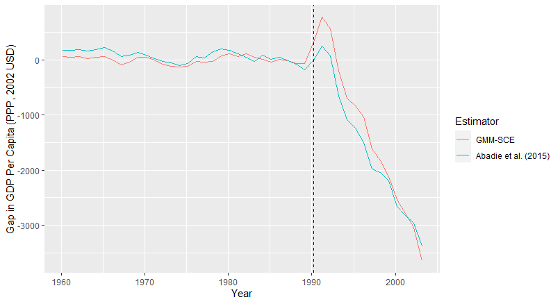
Figure 1: Gap between West Germany and Synthetic West Germany

To further facilitate comparison, when re-estimating the Synthetic West Germany, I use the same set of pre-treatment time periods. For my main specification, I use the two-step feasible version of the GMM-SCE so $A_{T_{0}}=\hat{\mathcal{V}}(\hat{W})^{-1}$ but I obtain similar results when $A_{T_{0}}=I_{K+1}$. Using this GMM-SCE, only five countries receive weight greater than one percent in the Synthetic West Germany, and they are: United States (.42), Austria (.28), Belgium (.12), Switzerland (.07), and Greece (.12). This is fairly similar to the Synthetic West Germany from Abadie et al. (2015) with the U.S., Austria, and Switzerland still receiving weight. Using this SC as the counterfactual, GDP per capita was reduced by approximately 1300 USD (2002) on average from 1990 to 2003 in West Germany due to German Reunification. The fact that this method gives a similar estimate of the average effect on GDP per capita provides evidence of the robustness of the original finding. Gaps between the Synthetic West Germany and the actual West Germany for both the original SCE and the GMM-SCE are given in Figure 1. As illustrated in the figure, the main reason why the estimated magnitude of the average treatment effect is lower using the GMM-SCE is because it estimates a larger positive effect in the years immediately after reunification, in fact a more than 3 times larger positive effect in 1991. However, as more time after reunification passes, the treatment effect estimates get closer and closer to one another.

6 Discussion

So far, when comparing this SCE to other panel methods I have focused on the fact that it has better formal guarantees when the number of time periods is large but the number of units is fixed. However, there are a number of other considerations to take into account when choosing between different panel methods. Firstly, there are also differences in the restrictions placed on the idiosyncratic shocks in the formal results. For example, Bai (2009) shows that when the factor structure is estimated using Principal Components, the factor structure can be consistently estimated even in the presence of serial correlation and heteroscedasticity in both dimensions, but there can be bias asymptotically unless it is imposed that there is no heteroscedasticity and no serial correlation in the idiosyncratic shocks along at least one of the dimensions. As a result, the conditions that are placed on the idiosyncratic shocks to obtain the asymptotic unbiasedness result here are weaker in terms of allowing the idiosyncratic shocks to be heteroskedastic in both dimensions and allowing serial correlation over time. Another consideration is how robust these methods are to being incorrect about the number of factors $F$. While asymptotic results for estimating the factor structure directly generally assume that $F$ is known, this method instead only requires that an upper bound on $F$ is known to ensure that $F\leq K+1$.

Another issue to consider is whether extrapolation is warranted. The standard justification for including the convexity constraints in SCEs is to prevent bias due to over-extrapolation. However, when $\mu_{0}\notin\mathcal{M}_{J}$, these constraints have the potential to lead to asymptotic bias because the unit of interest’s factor loadings cannot be reconstructed. Whereas, there is no such problem with a method that estimates the SC as a linear combination of the control units, provided that $J\geq F$. It is worth noting that there is an intuition that some applied researchers may have in this context that is captured by the notion of extrapolation bias. Roughly speaking that, all else equal, a SC that achieves good fit in the pre-treatment time periods is more likely to also have counterfactually achieved good fit in the post-treatment time periods if it did so without placing weights on the control units that are much larger than one or much less than zero. However, there is nothing in Assumption 1 that implies that extrapolation isn’t actually warranted. As a result, the linear factor model is not a complete justification for this intuition unless it is additionally assumed that the unit of interest’s factor loadings are in the convex hull of the control units’ factor loadings. However, there are other additional conditions that could be placed on the model that would provide some justification for these constraints. For example, if one assumes that all units have equal exposure to one of the factors, as is done in the two-way fixed effect model, then this can provide a justification for including the constraint that $\sum_{j\in\mathcal{J}}W_{j}=1$. This is because this constraint guarantees that the SC will have the same loading on this factor as the unit of interest in this case. Even if these constraints do not reduce the asymptotic bias, they may still function as regularization devices as discussed by Doudchenko and Imbens (2017), Ferman (2021), and Li (2020), particularly in the case where $J$ is large.

Appendix A. Proofs of the Main Results

Lemma 1 Suppose that Assumptions 1 and 2 hold. Additionally, $A_{T_{0}}\overset{p}{\rightarrow}A$ where $A$ is positive definite, and $T_{0}\rightarrow\infty$ while either

1. $J$ is fixed and $\mu_{0}\in\mathcal{M}_{J}$ or

2. $J\rightarrow\infty$ and $\mu_{0}\in\mathcal{M}$.

For $\hat{\mu}_{0}\equiv\mu_{\mathcal{J}}\hat{W}$ where $\hat{W}$ is defined by equation (1), $||\hat{\mu}_{0}-\mu_{0}||_{2}\overset{p}{\rightarrow}0$.

Proof: I first consider the case where $J$ is fixed and $\mu_{0}\in\mathcal{M}_{J}$. Let

$$H(W)=(\mu_{0}-\mu_{\mathcal{J}}W)^{\prime}\Lambda^{\prime}A\Lambda(\mu_{0}-\mu_{\mathcal{J}}W).$$

Let $\mathcal{W}^{*}=\operatorname*{arg\,min}_{W\in\Delta^{J}}H(W)$. Note that since $\mu_{0}\in\mathcal{M}_{J}$, $A$ is positive definite, and $rank(\Lambda)=F$, $\mu_{0}=\mu_{\mathcal{J}}W^{*}\;\text{for all }W^{*}\in\mathcal{W}^{*}$.

By Assumption 2,

$$\frac{1}{T_{0}}\tilde{Y}_{\mathcal{K}}^{pre}Y_{i}^{pre^{\prime}}\overset{p}{\rightarrow}\Lambda\mu_{i}\;\text{for all }i\in\{0,1,...,J\}.$$

Let $H_{T_{0}}(W)$ be equal to the objective function from equation (1). Note that by the triangle inequality, $\max_{W\in\Delta^{J}}||\Lambda(\mu_{0}-\mu_{\mathcal{J}}W)-\frac{1}{T_{0}}\tilde{Y}_{\mathcal{K}}^{pre}(Y_{0}^{pre^{\prime}}-Y_{\mathcal{J}}^{pre^{\prime}}W)||_{2}\leq 2\max_{i\in\{0,1,...,J\}}||\Lambda\mu_{i}-\frac{1}{T_{0}}\tilde{Y}_{\mathcal{K}}^{pre}Y_{i}^{pre}||_{2}=o_{p}(1)$. This implies that $\max_{W\in\Delta^{J}}||\frac{1}{T_{0}}\tilde{Y}_{\mathcal{K}}^{pre}(Y_{0}^{pre^{\prime}}-Y_{\mathcal{J}}^{pre^{\prime}}W)||_{2}=O_{p}(1)$. Therefore, using the triangle inequality and the fact that the Frobenius norm is submultiplicative, $\max_{W\in\Delta^{J}}|H(W)-H_{T_{0}}(W)|\leq\max_{W\in\Delta^{J}}2||\frac{1}{T_{0}}\tilde{Y}_{\mathcal{K}}^{pre}(Y_{0}^{pre^{\prime}}-Y_{\mathcal{J}}^{pre^{\prime}}W)||_{2}||A-A_{T_{0}}||_{2}+||\frac{1}{T_{0}}\tilde{Y}_{\mathcal{K}}^{pre}(Y_{0}^{pre^{\prime}}-Y_{\mathcal{J}}^{pre^{\prime}}W)||_{2}||A||_{2}||\Lambda(\mu_{0}-\mu_{\mathcal{J}}W)-\frac{1}{T_{0}}\tilde{Y}_{\mathcal{K}}^{pre}(Y_{0}^{pre^{\prime}}-Y_{\mathcal{J}}^{pre^{\prime}}W)||_{2}+||\Lambda(\mu_{0}-\mu_{\mathcal{J}}W)||_{2}||A||_{2}||\Lambda(\mu_{0}-\mu_{\mathcal{J}}W)-\frac{1}{T_{0}}\tilde{Y}_{\mathcal{K}}^{pre}(Y_{0}^{pre^{\prime}}-Y_{\mathcal{J}}^{pre^{\prime}}W)||_{2}=o_{p}(1)$ because $||A-A_{T_{0}}||_{2}=o_{p}(1)$. Therefore, $H_{T_{0}}(W)$ converges uniformly in probability to $H(W)$ for $W\in\Delta^{J}$.

Since $H(W)$ is continuous and $\Delta^{J}$ is compact, I follow Theorem 2.1 from Newey and McFadden (1994) to show that this implies $||\hat{\mu}_{0}-\mu_{0}||_{2}=o_{p}(1)$. Let $\eta>0$ and $W^{*}\in\mathcal{W}^{*}$. With probability approaching one (wpa1), $H_{T_{0}}(\hat{W})<H_{T_{0}}(W^{*})+\frac{\eta}{3}$ since $\hat{W}=\operatorname*{arg\,min}_{W\in\Delta^{J}}H_{T_{0}}(W)$. From uniform convergence in probability, $H(\hat{W})<H_{T_{0}}(\hat{W})+\frac{\eta}{3}$ and $H_{T_{0}}(W^{*})<H(W^{*})+\frac{\eta}{3}$ wpa1. Combining these three inequalities gives $H(\hat{W})<H(W^{*})+\eta$ wpa1. Now let $\delta>0$ and define the open set $\mathcal{V}=\{W\;|\;\exists W^{*}\in\mathcal{W}^{*}\text{ s.t. }||W^{*}-W||_{2}<\delta\}$. Since $\Delta^{J}$ is compact, so is $\Delta^{J}\cap\mathcal{V}^{c}$. Then since $H(W)$ is continuous, I can define a vector $\tilde{W}$ taking values in $\Delta^{J}\cap\mathcal{V}^{c}$ such that $\inf_{W\in\Delta^{J}\cap\mathcal{V}^{c}}H(W)=H(\tilde{W})>H(W^{*})$. Letting $\eta=H(\tilde{W})-H(W^{*})\;\text{for all }W^{*}\in\mathcal{W}^{*}$, then we have that wpa1 $H(\hat{W})<H(W^{*})+\eta=H(\tilde{W})$ which implies that $\hat{W}\in\mathcal{V}$ wpa1. Then $\inf_{W^{*}\in\mathcal{W}^{*}}||\hat{W}-W^{*}||_{2}\overset{p}{\rightarrow}0$. Therefore, $||\hat{\mu}_{0}-\mu_{0}||_{2}=\inf_{W^{*}\in\mathcal{W}^{*}}||\mu_{\mathcal{J}}\hat{W}-\mu_{\mathcal{J}}W^{*}||_{2}\leq||\mu_{\mathcal{J}}||_{2}\inf_{W^{*}\in\mathcal{W}^{*}}||\hat{W}-W^{*}||_{2}\overset{p}{\rightarrow}0$.

For the case where $J\rightarrow\infty$ and $\mu_{0}\in\mathcal{M}$, I follow the approach used in Proposition 3.1 of Ferman (2021) by reformulating the optimization problem to choose the control weights in equation (1) as one to choose the factor loadings of the Synthetic Control. I make the feasible set equal to $\mathcal{M}$ instead of $\Delta^{J}$ so it no longer depends on $J$ and note that $\mathcal{M}$ is compact by Assumption 2.3 and $||W||_{1}=1$. Then instead of using the objective function from equation (1), I use the alternative objective function given below:

$$H_{J}(\mu)=\min_{\tilde{\mu}\in\mathcal{M}_{J}}\{\min_{W\in\Delta^{J}:\mu_{\mathcal{J}}W=\tilde{\mu}}\{(\frac{1}{T_{0}}\tilde{Y}_{\mathcal{K}}^{pre}(Y_{0}^{pre^{\prime}}-Y_{\mathcal{J}}^{pre^{\prime}}W))^{\prime}A_{T_{0}}(\frac{1}{T_{0}}\tilde{Y}_{\mathcal{K}}^{pre}(Y_{0}^{pre^{\prime}}-Y_{\mathcal{J}}^{pre^{\prime}}W))\}+K||\mu-\tilde{\mu}||_{2}\}.$$

$K$ will be defined later in the proof but for now it suffices to note that $K>0$ and $K=O_{p}(1)$. Then it will be the case that for $\hat{W}$ defined in equation (1), $\mu_{\mathcal{J}}\hat{W}\equiv\hat{\mu}_{0}=\operatorname*{arg\,min}_{\mu\in\mathcal{M}}H_{J}(\mu)$. Let $H(\mu)=(\mu_{0}-\mu)^{\prime}\Lambda^{\prime}A\Lambda(\mu_{0}-\mu)$ and $\{W^{J}\}_{J\in\mathbb{N}}$ with $W^{J}\in\Delta^{J}\;\text{for all }J$ be a sequence of control weights such that for $\mu^{J}\equiv\mu_{\mathcal{J}}W^{J}$, $\lim_{J\rightarrow\infty}||\mu_{0}-\mu^{J}||_{2}=0$. Such a sequence of weights will exist because $\mu_{0}\in\mathcal{M}$. I first show that a sequence of functions which upper bounds $H_{J}(\mu)$ converges in probability to $H(\mu)$ at $\mu=\mu_{0}$. I define this upper bound as:

$$H^{UB}_{J}(\mu)=(\frac{1}{T_{0}}\tilde{Y}_{\mathcal{K}}^{pre}(Y_{0}^{pre^{\prime}}-Y_{\mathcal{J}}^{pre^{\prime}}W^{J}))^{\prime}A_{T_{0}}(\frac{1}{T_{0}}\tilde{Y}_{\mathcal{K}}^{pre}(Y_{0}^{pre^{\prime}}-Y_{\mathcal{J}}^{pre^{\prime}}W^{J}))+K||\mu-\mu^{J}||_{2}.$$

Since $W^{J}$ and $\mu^{J}$ form a pair of feasible solutions to the inner and outer minimization problems in $H_{J}(\mu)$ respectively, it must be the case that $H_{J}(\mu)\leq H_{J}^{UB}(\mu)\;\text{for all }\mu\in\mathcal{M}$. Since $\lim_{J\rightarrow\infty}||\mu_{0}-\mu^{J}||_{2}=0$ and $K=O_{p}(1)$, $K||\mu_{0}-\mu^{J}||_{2}=o_{p}(1)$. Note that

$$||\frac{1}{T_{0}}\tilde{Y}_{\mathcal{K}}^{pre}(\lambda^{pre}(\mu_{0}-\mu_{\mathcal{J}}W^{J})+\epsilon_{0}^{pre^{\prime}}-\epsilon_{\mathcal{J}}^{pre^{\prime}}W^{J})||_{2}\leq||\frac{1}{T_{0}}\tilde{Y}_{\mathcal{K}}^{pre}\lambda^{pre}||_{2}||\mu_{0}-\mu_{\mathcal{J}}W^{J}||_{2}+||\frac{1}{T_{0}}\epsilon_{0}^{pre^{\prime}}||_{2}+$$

$$\max_{j\in\mathcal{J}}||\frac{1}{T_{0}}\tilde{Y}_{\mathcal{K}}^{pre}\epsilon_{j}^{pre^{\prime}}||_{2}=O_{p}(1)||\mu_{0}-\mu_{\mathcal{J}}W||_{2}+o_{p}(1)$$

by Assumption 2. Then since $||\mu_{0}-\mu_{\mathcal{J}}W^{J}||_{2}=o(1)$, $|H_{J}^{UB}(\mu_{0})|=o_{p}(1)$. Therefore, because $H(\mu_{0})=0$, $|H_{J}^{UB}(\mu_{0})-H(\mu_{0})|=o_{p}(1)$.

Next, I show that a sequence of functions which lower bounds $H_{J}(\mu)$ converges uniformly in probability to $H(\mu)$. I define this sequence of functions as

$$H^{LB}_{J}(\mu)=\min_{\tilde{\mu}\in\mathcal{M}}\{Q_{J}(\tilde{\mu})+K||\mu-\tilde{\mu}||_{2}\}$$

where $Q_{J}(\tilde{\mu})=\min_{b\in\mathcal{W}}\{(\frac{1}{T_{0}}\tilde{Y}_{\mathcal{K}}^{pre}(Y_{0}^{pre^{\prime}}-\lambda^{pre}\tilde{\mu}-\epsilon_{\mathcal{J}}^{pre^{\prime}}b))^{\prime}A_{T_{0}}(\frac{1}{T_{0}}\tilde{Y}_{\mathcal{K}}^{pre}(Y_{0}^{pre^{\prime}}-\lambda^{pre}\tilde{\mu}-\epsilon_{\mathcal{J}}^{pre^{\prime}}b))\}$ and $\mathcal{W}=\{b:||b||_{1}\leq 1\}$. Note that this is the same way that $H_{J}(\mu)$ is defined except for the feasible set for the outer minimization problem is now $\mathcal{M}\supseteq\mathcal{M}_{J}$ and the feasible set for the inner minimization problem has also been expanded since $\mathcal{W}=\{W:||W||_{1}\leq 1\}\supset\{W\in\Delta^{J}:\mu_{\mathcal{J}}W=\tilde{\mu}\}$ which implies that $H_{J}(\mu)\geq H^{LB}_{J}(\mu)\;\text{for all }\mu\in\mathcal{M}$. In order to show uniform convergence in probability, I first show that the function $Q_{J}(\tilde{\mu})$ is Lipschitz with a constant that is $O_{p}(1)$. Since $\mathcal{M}$ is convex and $Q_{J}(\tilde{\mu})$ is differentiable by the Envelope Theorem, by the Mean Value Theorem $\text{for all }\mu,\mu^{\prime}\in\mathcal{M}$, $\exists\bar{\mu}\in\mathcal{M}$ such that

$$|Q_{J}(\mu)-Q_{J}(\mu^{\prime})|=|Q_{J}^{\prime}(\bar{\mu})(\mu-\mu^{\prime})|\leq||Q_{J}^{\prime}(\bar{\mu})||_{2}||\mu-\mu^{\prime}||_{2}$$

where the inequality follows from the Cauchy-Schwartz Inequality. Let $\hat{b}(\tilde{\mu})=\operatorname*{arg\,min}_{b\in\mathcal{W}}Q_{J}(\tilde{\mu})$. Then using the Envelope Theorem,

$$||Q_{J}^{\prime}(\bar{\mu})||_{2}||\mu-\mu^{\prime}||_{2}=||(\frac{1}{T_{0}}\tilde{Y}_{\mathcal{K}}^{pre}(Y_{0}^{pre^{\prime}}-\lambda^{pre}\bar{\mu}-\epsilon_{\mathcal{J}}^{pre^{\prime}}\hat{b}(\bar{\mu}))(A_{T_{0}}+A_{T_{0}}^{\prime})(-\frac{1}{T_{0}}\tilde{Y}_{\mathcal{K}}^{pre}\lambda^{pre})||_{2}|||\mu-\mu^{\prime}||_{2}$$

$$\leq||\frac{1}{T_{0}}\tilde{Y}_{\mathcal{K}}^{pre}(Y_{0}^{pre^{\prime}}-\lambda^{pre}\bar{\mu}-\epsilon_{\mathcal{J}}^{pre^{\prime}}\hat{b}(\bar{\mu})||_{2}||A_{T_{0}}+A_{T_{0}}^{\prime}||_{2}||\frac{1}{T_{0}}\tilde{Y}_{\mathcal{K}}^{pre}\lambda^{pre}||_{2}||\mu-\mu^{\prime}||_{2}$$

where $||\frac{1}{T_{0}}\tilde{Y}_{\mathcal{K}}^{pre}\lambda^{pre}||_{2}\overset{p}{\rightarrow}||\Lambda||_{2}$ by Assumption 2, $\max_{\mu,\mu^{\prime}\in\mathcal{M}}||\mu-\mu^{\prime}||_{2}=O(1)$ since $\mathcal{M}$ is compact, and $||A_{T_{0}}+A_{T_{0}}^{\prime}||_{2}=O_{p}(1)$ since $A_{T_{0}}\overset{p}{\rightarrow}A$. Using the the Triangle Inequality and $||\hat{b}(\tilde{\mu})||_{1}\leq 1$,

$$||\frac{1}{T_{0}}\tilde{Y}_{\mathcal{K}}^{pre}(Y_{0}^{pre^{\prime}}-\lambda^{pre}\bar{\mu}-\epsilon_{\mathcal{J}}^{pre^{\prime}}\hat{b}(\bar{\mu})||_{2}\leq||\frac{1}{T_{0}}\tilde{Y}_{\mathcal{K}}^{pre}Y_{0}^{pre^{\prime}}||_{2}+||\frac{1}{T_{0}}\tilde{Y}_{\mathcal{K}}^{pre}\lambda^{pre}\bar{\mu}||_{2}+\max_{j\in\mathcal{J}}||\frac{1}{T_{0}}\tilde{Y}_{\mathcal{K}}^{pre}\epsilon_{j}^{pre^{\prime}}||_{2}.$$

Using Assumption 2, $||\frac{1}{T_{0}}\tilde{Y}_{\mathcal{K}}^{pre}Y_{0}^{pre^{\prime}}||_{2}\overset{p}{\rightarrow}||\Lambda\mu_{0}||_{2}$, $\max_{\bar{\mu}\in\mathcal{M}}||\frac{1}{T_{0}}\tilde{Y}_{\mathcal{K}}^{pre}\lambda^{pre}\bar{\mu}||_{2}\leq||\frac{1}{T_{0}}\tilde{Y}_{\mathcal{K}}^{pre}\lambda^{pre}||_{2}\max_{\bar{\mu}\in\mathcal{M}}||\bar{\mu}||_{2}\overset{p}{\rightarrow}||\Lambda||_{2}\max_{\bar{\mu}\in\mathcal{M}}||\bar{\mu}||_{2}$, and $\max_{j\in\mathcal{J}}||\frac{1}{T_{0}}\tilde{Y}_{\mathcal{K}}^{pre}\epsilon_{j}^{pre^{\prime}}|||_{2}\overset{p}{\rightarrow}0$. Therefore, I can define $\tilde{K}$ as

$$\tilde{K}=(||\frac{1}{T_{0}}\tilde{Y}_{\mathcal{K}}^{pre}Y_{0}^{pre^{\prime}}||_{2}+||\frac{1}{T_{0}}\tilde{Y}_{\mathcal{K}}^{pre}\lambda^{pre}||_{2}\max_{\bar{\mu}\in\mathcal{M}}||\bar{\mu}||_{2}+\max_{j\in\mathcal{J}}||\frac{1}{T_{0}}\tilde{Y}_{\mathcal{K}}^{pre}\epsilon_{j}^{pre^{\prime}}||_{2})||A_{T_{0}}+A_{T_{0}}^{\prime}||_{2}||\frac{1}{T_{0}}\tilde{Y}_{\mathcal{K}}^{pre}\lambda^{pre}||_{2}.$$

Then there exists $\tilde{K}$ such that $|Q_{J}(\mu)-Q_{J}(\mu^{\prime})|\leq||Q_{J}^{\prime}(\bar{\mu})||_{2}||\mu-\mu^{\prime}||_{2}\leq\tilde{K}||\mu-\mu^{\prime}||_{2}$, $\tilde{K}=O_{p}(1)$, and it does not depend on $\mu$ and $\mu^{\prime}$. I now define the $K$ in $H_{J}(\mu)$ as $K=\tilde{K}+1$ so it is in fact the case that $K>0$ and $K=O_{p}(1)$. Because $K$ is greater than the Lipschitz constant of $Q_{J}(\mu)$, it will be the case that $H^{LB}_{J}(\mu)=Q_{J}(\mu)=(\frac{1}{T_{0}}\tilde{Y}_{\mathcal{K}}^{pre}(Y_{0}^{pre^{\prime}}-\lambda^{pre}\mu-\epsilon_{\mathcal{J}}^{pre^{\prime}}\hat{b}(\mu)))^{\prime}A_{T_{0}}(\frac{1}{T_{0}}\tilde{Y}_{\mathcal{K}}^{pre}(Y_{0}^{pre^{\prime}}-\lambda^{pre}\mu-\epsilon_{\mathcal{J}}^{pre^{\prime}}\hat{b}(\mu)))\;\text{for all }\mu\in\mathcal{M}$. Therefore $\sup_{\mu\in\mathcal{M}}|H^{LB}_{J}(\mu)-H(\mu)|=\sup_{\mu\in\mathcal{M}}|(\frac{1}{T_{0}}\tilde{Y}_{\mathcal{K}}^{pre}(Y_{0}^{pre^{\prime}}-\lambda^{pre}\mu-\epsilon_{\mathcal{J}}^{pre^{\prime}}\hat{b}(\mu)))^{\prime}A_{T_{0}}(\frac{1}{T_{0}}\tilde{Y}_{\mathcal{K}}^{pre}(Y_{0}^{pre^{\prime}}-\lambda^{pre}\mu-\epsilon_{\mathcal{J}}^{pre^{\prime}}\hat{b}(\mu)))-(\mu_{0}-\mu)^{\prime}\Lambda^{\prime}A\Lambda(\mu_{0}-\mu)|\leq\sup_{\mu\in\mathcal{M}}2||\frac{1}{T_{0}}\tilde{Y}_{\mathcal{K}}^{pre}(Y_{0}^{pre^{\prime}}-\lambda^{pre}\mu-\epsilon_{\mathcal{J}}^{pre^{\prime}}\hat{b}(\mu))||_{2}||A-A_{T_{0}}||_{2}+||\frac{1}{T_{0}}\tilde{Y}_{\mathcal{K}}^{pre}(Y_{0}^{pre^{\prime}}-\lambda^{pre}\mu-\epsilon_{\mathcal{J}}^{pre^{\prime}}\hat{b}(\mu))||_{2}||A||_{2}||\Lambda(\mu_{0}-\mu)-\frac{1}{T_{0}}\tilde{Y}_{\mathcal{K}}^{pre}(Y_{0}^{pre^{\prime}}-\lambda^{pre}\mu-\epsilon_{\mathcal{J}}^{pre^{\prime}}\hat{b}(\mu))||_{2}+||\Lambda(\mu_{0}-\mu)||_{2}||A||_{2}||\Lambda(\mu_{0}-\mu)-\frac{1}{T_{0}}\tilde{Y}_{\mathcal{K}}^{pre}(Y_{0}^{pre^{\prime}}-\lambda^{pre}\mu-\epsilon_{\mathcal{J}}^{pre^{\prime}}\hat{b}(\mu))||_{2}$. Again using Assumption 2 and $||\hat{b}(\mu)||_{1}\leq 1$,

$$\sup_{\mu\in\mathcal{M}}||\Lambda(\mu_{0}-\mu)-\frac{1}{T_{0}}\tilde{Y}_{\mathcal{K}}^{pre}(\lambda^{pre}(\mu_{0}-\mu)+\epsilon_{0}^{pre^{\prime}}-\epsilon_{\mathcal{J}}^{pre^{\prime}}\hat{b}(\mu))||_{2}\leq$$

$$\sup_{\mu\in\mathcal{M}}||\Lambda-\tilde{Y}_{\mathcal{K}}^{pre}\lambda^{pre}||_{2}||\mu_{0}-\mu||_{2}+||\tilde{Y}_{\mathcal{K}}^{pre}\epsilon_{0}^{\prime}||_{2}+\max_{j\in\mathcal{J}}||\tilde{Y}_{\mathcal{K}}^{pre}\epsilon_{j}^{\prime}||_{2}=o_{p}(1).$$

This also implies that $\sup_{\mu\in\mathcal{M}}||\frac{1}{T_{0}}\tilde{Y}_{\mathcal{K}}^{pre}(Y_{0}^{pre^{\prime}}-\lambda^{pre}\mu-\epsilon_{\mathcal{J}}^{pre^{\prime}}\hat{b}(\mu))||_{2}=O_{p}(1)$. Combining this with $||A_{T_{0}}-A||_{2}=o_{p}(1)$ gives us that $\sup_{\mu\in\mathcal{M}}|H_{J}^{LB}(\mu)-H(\mu)|=o_{p}(1)$.

Lastly, I again use an extension of Theorem 2.1 from Newey and McFadden (1994) to show that $(i)H_{J}(\mu_{0})\leq H^{UB}_{J}(\mu_{0})$ with $|H^{UB}_{J}(\mu_{0})-H(\mu_{0})|\overset{p}{\rightarrow}0$ and $(ii)H_{J}(\mu)\geq H^{LB}_{J}(\mu)$ with $\sup_{\mu\in\mathcal{M}}|H^{LB}_{J}(\mu)-H(\mu)|\overset{p}{\rightarrow}0$ together imply $||\hat{\mu}_{0}-\mu_{0}||_{2}=o_{p}(1)$. Let $\eta>0$. $H_{J}(\hat{\mu}_{0})<H_{J}(\mu_{0})+\frac{\eta}{3}$ wpa1 since $\hat{\mu}_{0}=\operatorname*{arg\,min}_{\mu\in\mathcal{M}}H_{J}(\mu)$. From (ii), $H(\hat{\mu}_{0})<H^{LB}_{J}(\hat{\mu}_{0})+\frac{\eta}{3}\leq H_{J}(\hat{\mu}_{0})+\frac{\eta}{3}$ wpa1. Together (i) and (ii) imply that $H_{J}(\mu_{0})\overset{p}{\rightarrow}H(\mu_{0})$ which means that $H_{J}(\mu_{0})<H(\mu_{0})+\frac{\eta}{3}$ wpa1. Combining these three inequalities gives $H(\hat{\mu}_{0})<H(\mu_{0})+\eta$ wpa1. Now let $\delta>0$ and let $\mathcal{V}=\{\mu\;|\;||\mu-\mu_{0}||_{2}<\delta\}$. Since $\mathcal{M}$ is compact, so is $\mathcal{M}\cap\mathcal{V}^{c}$. Note that $\mu_{0}$ is the unique minimum of $H(\mu)$ as a result of $rank(\Lambda)=F$, $A$ being positive definite, and $\mu_{0}\in\mathcal{M}$. Because $\mu_{0}$ is the unique minimum of $H(\mu)$ and $H(\mu)$ is continuous, I can define a vector $\tilde{\mu}$ taking values in $\mathcal{M}\cap\mathcal{V}^{c}$ such that $\inf_{\mu\in\mathcal{M}\cap\mathcal{V}^{c}}H(\mu)=H(\tilde{\mu})>H(\mu_{0})$. Letting $\eta=H(\tilde{\mu})-H(\mu_{0})$, then we have that wpa1 $H(\hat{\mu}_{0})<H(\mu_{0})+\eta=H(\tilde{\mu})$ which implies that $\hat{\mu}_{0}\in\mathcal{V}$ wpa1. Therefore $||\hat{\mu}_{0}-\mu_{0}||_{2}\overset{p}{\rightarrow}0$.

Proposition 1 Suppose that Assumptions 1 and 2 are satisfied, $A_{T_{0}}\overset{p}{\rightarrow}A$ where $A$ is positive definite, and $T_{0}\rightarrow\infty$ while either

1. $J$ is fixed and $\mu_{0}\in\mathcal{M}_{J}$ or

2. $J\rightarrow\infty$, $\mu_{0}\in\mathcal{M}$, and $\epsilon_{\mathcal{J}}^{post}\rotatebox[origin={c}]{90.0}{$\models$}Y^{pre}$.

Then $\text{for all }t\in\mathcal{T}_{1},\;\lim_{T_{0}\rightarrow\infty}E[\hat{\alpha}_{0t}]=E[\alpha_{0t}]$.

Proof: We can first note that by $\hat{W}\in\Delta^{J}$ and Assumption 2.3, $||\hat{\mu}_{0}-\mu_{0}||_{2}$ is bounded. Therefore, since $||\hat{\mu}_{0}-\mu_{0}||_{2}=o_{p}(1)$ by Lemma 1, $\lim_{T_{0}\rightarrow\infty}E[||\hat{\mu}_{0}-\mu_{0}||_{2}^{2}]=0$. $E[\hat{\alpha}_{0t}-\alpha_{0t}]=E[\lambda_{t}(\mu_{0}-\hat{\mu}_{0})+\epsilon_{0t}-\sum_{j\in\mathcal{J}}\hat{W}_{j}\epsilon_{jt}]$. $|E[\lambda_{t}(\mu_{0}-\hat{\mu}_{0})]|\leq E[|\lambda_{t}(\mu_{0}-\hat{\mu}_{0})|]\leq E[||\lambda_{t}||_{2}||\mu_{0}-\hat{\mu}_{0}||_{2}|]\leq E[||\lambda_{t}||_{2}^{2}]^{\frac{1}{2}}E[||\mu_{0}-\hat{\mu}_{0}||_{2}^{2}]^{\frac{1}{2}}\rightarrow 0$ as $T_{0}\rightarrow\infty$ using the Cauchy-Schwartz Inequality. For case (i), let $\mathcal{W}^{*}\equiv\{W\;:\;\mu_{\mathcal{J}}W=\mu_{0}\}$. Then as shown in the proof of Lemma 1, $\inf_{W\in\mathcal{W}^{*}}||\hat{W}-W||_{2}=o_{p}(1)$ and because this is bounded $\inf_{W\in\mathcal{W}^{*}}E||\hat{W}-W||_{2}^{2}]\rightarrow 0$ as $T_{0}\rightarrow\infty$. Note that for each $W\in\mathcal{W}^{*}$,

$$|E[\sum_{j\in\mathcal{J}}\hat{W}_{j}\epsilon_{jt}]|=|E[\sum_{j\in\mathcal{J}}(\hat{W}_{j}-W_{j})\epsilon_{jt}]+E[\sum_{j\in\mathcal{J}}W_{j}\epsilon_{jt}]|=|E[\sum_{j\in\mathcal{J}}(\hat{W}_{j}-W_{j})\epsilon_{jt}]|$$

$$\leq E||\hat{W}-W||_{2}^{2}]^{\frac{1}{2}}E[||\sum_{j\in\mathcal{J}}\epsilon_{jt}||_{2}^{2}]^{\frac{1}{2}}.$$

Therefore $|E[\sum_{j\in\mathcal{J}}\hat{W}_{j}\epsilon_{jt}]|\leq\inf_{W\in\mathcal{W^{*}}}E||\hat{W}-W||_{2}^{2}]^{\frac{1}{2}}E[||\sum_{j\in\mathcal{J}}\epsilon_{jt}||_{2}^{2}]^{\frac{1}{2}}\rightarrow 0$ as $T_{0}\rightarrow\infty$ while $J$ is fixed. For case (ii), because $\hat{W}_{j}\;\text{for all }j\in\mathcal{J}$ is a bounded measurable function of $Y^{pre}$ which is independent of $\epsilon_{\mathcal{J}}^{post}$, $E[\sum_{j\in\mathcal{J}}\hat{W}_{j}\epsilon_{jt}]=0$. Therefore, in both cases we have

$$|E[\hat{\alpha}_{0t}-\alpha_{0t}]|=|E[\lambda_{t}(\hat{\mu}_{0}-\mu_{0})+\epsilon_{0t}-\sum_{j\in\mathcal{J}}\hat{W}_{j}\epsilon_{jt}]|\leq|E[\lambda_{t}(\hat{\mu}_{0}-\mu_{0})]|+|E[\sum_{j\in\mathcal{J}}\hat{W}_{j}\epsilon_{jt}]|\rightarrow 0\text{ as }T_{0}\rightarrow\infty.$$

Proposition 2 Suppose that Assumptions 1, 2, and 3 are satisfied, $A_{T_{0}}\overset{p}{\rightarrow}A$ where $A$ is positive definite, and $T_{0},T_{1}\rightarrow\infty$ while either

1. $J$ is fixed and $\mu_{0}\in\mathcal{M}_{J}$

2. $J\rightarrow\infty$ and $\mu_{0}\in\mathcal{M}$

Then $\sum_{t\in\mathcal{T}_{1}}v_{t}^{T_{1}}(\alpha_{0t}-\hat{\alpha}_{0t})\overset{p}{\rightarrow}0$.

Proof: First note that since $\sup_{t\in\mathcal{T}_{1}}E[||\lambda_{t}||_{2}^{2}]<\infty$ and $v^{T_{1}}\in\Delta^{T_{1}}$, then $\text{for all }f\in\{1,...,F\}$, $\text{for all }\eta>0$,

$$P(|\sum_{t\in\mathcal{T}_{1}}v_{t}^{T_{1}}\lambda_{tf}|>\eta)\leq\frac{E[(\sum_{t\in\mathcal{T}_{1}}v_{t}^{T_{1}}\lambda_{tf})^{2}]}{\eta^{2}}\leq\frac{\sum_{t\in\mathcal{T}_{1}}\sum_{s\in\mathcal{T}_{1}}v_{t}^{T_{1}}v_{s}^{T_{1}}E[\lambda_{tf}\lambda_{sf}]}{\eta^{2}}\leq\frac{\sup_{t\in\mathcal{T}_{1}}E[\lambda_{tf}^{2}]}{\eta^{2}}.$$

Therefore, $\sum_{t\in\mathcal{T}_{1}}v_{t}^{T_{1}}\lambda_{tf}=O_{p}(1)\;\text{for all }\{1,...,F\}$. $\sum_{t\in\mathcal{T}_{1}}v_{t}^{T_{1}}(\hat{\alpha}_{0t}-\alpha_{0t})$ is equal to

$$\sum_{t\in\mathcal{T}_{1}}v_{t}^{T_{1}}(\lambda_{t}(\mu_{0}-\hat{\mu}_{0})+\epsilon_{0t}-\sum_{j\in\mathcal{J}}\hat{W}_{j}\epsilon_{jt})=(\sum_{t\in\mathcal{T}_{1}}v_{t}^{T_{1}}\lambda_{t})(\mu_{0}-\hat{\mu}_{0})+\sum_{t\in\mathcal{T}_{1}}v_{t}^{T_{1}}\epsilon_{0t}-\sum_{j\in\mathcal{J}}\hat{W}_{j}\sum_{t\in\mathcal{T}_{1}}v_{t}^{T_{1}}\epsilon_{jt}.$$

Using Assumption 3, $\sum_{t\in\mathcal{T}_{1}}v_{t}^{T_{1}}\epsilon_{0t}=o_{p}(1)$, and $|\sum_{j\in\mathcal{J}}\hat{W}_{j}\sum_{t\in\mathcal{T}_{1}}v_{t}^{T_{1}}\epsilon_{jt}|\leq\max_{j\in\mathcal{J}}|\sum_{t\in\mathcal{T}_{1}}v_{t}^{T_{1}}\epsilon_{jt}|=o_{p}(1)$ where the inequality comes from the fact that $||\hat{W}||_{1}=1$. Because $||\mu_{0}-\hat{\mu}_{0}||_{2}=o_{p}(1)$ by Lemma 1, $|(\sum_{t\in\mathcal{T}_{1}}v_{t}^{T_{1}}\lambda_{t})(\mu_{0}-\hat{\mu}_{0})|\leq||\sum_{t\in\mathcal{T}_{1}}v_{t}^{T_{1}}\lambda_{t}||_{2}||\mu_{0}-\hat{\mu}_{0}||_{2}=O_{p}(1)o_{p}(1)=o_{p}(1)$. Therefore, we have that $\sum_{t\in\mathcal{T}_{1}}v_{t}^{T_{1}}(\alpha_{0t}-\hat{\alpha}_{0t})=o_{p}(1)$.

Lemma 2 Suppose that the conditions of Assumptions 1, 2, and 4 are satisfied, $A_{T_{0}}\overset{p}{\rightarrow}A$ where $A$ is positive definite, and $T_{0}\rightarrow\infty$ while $J$ is fixed. Then,

$$\sqrt{T_{0}}(\hat{\mu}_{0}-\mu_{0})\overset{d}{\rightarrow}\Pi_{T_{\mathcal{M}_{J}}(\mu_{0})}(Z_{1})\text{ where }$$

$$Z_{1}\sim N(0,(\Lambda^{\prime}A\Lambda\mu_{\mathcal{J}}\mu_{\mathcal{J}}^{\prime}\Lambda^{\prime}A\Lambda)^{-1}\Lambda^{\prime}A\Lambda\mu_{\mathcal{J}}\mu_{\mathcal{J}}^{\prime}\Lambda^{\prime}A\mathcal{V}A\Lambda\mu_{\mathcal{J}}\mu_{\mathcal{J}}^{\prime}\Lambda^{\prime}A\Lambda(\Lambda^{\prime}A\Lambda\mu_{\mathcal{J}}\mu_{\mathcal{J}}^{\prime}\Lambda^{\prime}A\Lambda)^{-1}).$$

Proof: Let the set of optimal solutions for the unconstrained estimator in equation (2) be denoted by

$$\mathcal{W}^{GMM}=\operatorname*{arg\,min}_{W}(\frac{1}{T_{0}}\tilde{Y}_{\mathcal{K}}^{pre}(Y_{0}^{pre^{\prime}}-Y_{\mathcal{J}}^{pre^{\prime}}\hat{W}^{GMM}))^{\prime}A_{T_{0}}(\frac{1}{T_{0}}\tilde{Y}_{\mathcal{K}}^{pre}(Y_{0}^{pre^{\prime}}-Y_{\mathcal{J}}^{pre^{\prime}}\hat{W}^{GMM}))$$

and because $\mathcal{W}^{GMM}$ is closed and convex, let $\hat{W}^{GMM}\in\operatorname*{arg\,min}_{W\in\mathcal{W}^{GMM}}||W-W^{*}||_{2}$. Note that $\hat{W}^{GMM}$ must satisfy the first-order condition,

$$\frac{1}{T_{0}}Y_{\mathcal{J}}^{pre}\tilde{Y}_{\mathcal{K}}^{pre^{\prime}}A_{T_{0}}(\frac{1}{T_{0}}\tilde{Y}_{\mathcal{K}}^{pre}(Y_{0}^{pre^{\prime}}-Y_{\mathcal{J}}^{pre^{\prime}}\hat{W}^{GMM}))=0.$$

Using the fact that

$$\frac{1}{T_{0}}\tilde{Y}_{\mathcal{K}}^{pre}(Y_{0}^{pre^{\prime}}-Y_{\mathcal{J}}^{pre^{\prime}}\hat{W}^{GMM})=\frac{1}{T_{0}}\tilde{Y}_{\mathcal{K}}^{pre}(Y_{0}^{pre^{\prime}}-Y_{\mathcal{J}}^{pre^{\prime}}W^{*})-\frac{1}{T_{0}}\tilde{Y}_{\mathcal{K}}^{pre}Y_{\mathcal{J}}^{pre^{\prime}}(\hat{W}^{GMM}-W^{*}),$$

we can rewrite the first-order condition as

$$\frac{1}{T_{0}}Y_{\mathcal{J}}^{pre}\tilde{Y}_{\mathcal{K}}^{pre^{\prime}}A_{T_{0}}\frac{1}{T_{0}}\tilde{Y}_{\mathcal{K}}^{pre}Y_{\mathcal{J}}^{pre^{\prime}}\sqrt{T_{0}}(\hat{W}^{GMM}-W^{*})=-\frac{1}{T_{0}}Y_{\mathcal{J}}^{pre}\tilde{Y}_{\mathcal{K}}^{pre}A_{T_{0}}(\frac{1}{\sqrt{T_{0}}}\tilde{Y}_{\mathcal{K}}^{pre}(Y_{0}^{pre^{\prime}}-Y_{\mathcal{J}}^{pre^{\prime}}W^{*})).$$

Expanding the left side of the equation,

$$\frac{1}{T_{0}}Y_{\mathcal{J}}^{pre}\tilde{Y}_{\mathcal{K}}^{pre^{\prime}}A_{T_{0}}(\frac{1}{T_{0}}\tilde{Y}_{\mathcal{K}}^{pre}(\lambda^{pre}\mu_{\mathcal{J}}+\epsilon_{\mathcal{J}}^{pre^{\prime}})\sqrt{T_{0}}(\hat{W}^{GMM}-W^{*})=-\frac{1}{T_{0}}Y_{\mathcal{J}}^{pre}\tilde{Y}_{\mathcal{K}}^{pre}A_{T_{0}}(\frac{1}{\sqrt{T_{0}}}\tilde{Y}_{\mathcal{K}}^{pre}(Y_{0}^{pre^{\prime}}-Y_{\mathcal{J}}^{pre^{\prime}}W^{*})).$$

By Assumption 2 and $A_{T_{0}}=O_{p}(1)$, $\max_{j\in\mathcal{J}}\frac{1}{T_{0}}Y_{\mathcal{J}}^{pre}\tilde{Y}_{\mathcal{K}}^{pre^{\prime}}A_{T_{0}}\frac{1}{T_{0}}\tilde{Y}_{\mathcal{K}}^{pre}\epsilon_{j}^{pre^{\prime}}=o_{p}(1)$ and I show in Lemma 4 in Appendix B that $\sqrt{T_{0}}||\hat{W}^{GMM}-W^{*}||_{2}=O_{p}(1)$, so $\frac{1}{T_{0}}Y_{\mathcal{J}}^{pre}\tilde{Y}_{\mathcal{K}}^{pre^{\prime}}A_{T_{0}}\frac{1}{T_{0}}\tilde{Y}_{\mathcal{K}}^{pre}\epsilon_{\mathcal{J}}^{pre^{\prime}}\sqrt{T_{0}}(\hat{W}^{GMM}-W^{*})=o_{p}(1)$. Therefore, $\sqrt{T_{0}}\mu_{\mathcal{J}}(\hat{W}^{GMM}-W^{*})$ is equal to

$$(\lambda^{pre^{\prime}}\tilde{Y}_{\mathcal{K}}^{pre^{\prime}}A_{T_{0}}\tilde{Y}_{\mathcal{K}}^{pre}Y_{\mathcal{J}}^{pre^{\prime}}Y_{\mathcal{J}}^{pre}\tilde{Y}_{\mathcal{K}}^{pre^{\prime}}A_{T_{0}}\tilde{Y}_{\mathcal{K}}^{pre}\lambda^{pre}/T_{0}^{4})^{-1}\frac{1}{T_{0}}Y_{\mathcal{J}}^{pre}\tilde{Y}_{\mathcal{K}}^{pre^{\prime}}A_{T_{0}}(\frac{1}{\sqrt{T_{0}}}\tilde{Y}_{\mathcal{K}}^{pre}(Y_{0}^{pre^{\prime}}-Y_{\mathcal{J}}^{pre^{\prime}}W^{*}))+o_{p}(1).$$

Then letting $\hat{\mu}_{0}^{GMM}=\mu_{\mathcal{J}}\hat{W}^{GMM}$ and using Assumptions 2 and 4 we have that

$$\sqrt{T_{0}}(\hat{\mu}_{0}^{GMM}-\mu_{0})\overset{d}{\rightarrow}Z_{1}\sim N(0,(\Lambda^{\prime}A\Lambda\mu_{\mathcal{J}}\mu_{\mathcal{J}}^{\prime}\Lambda^{\prime}A\Lambda)^{-1}\Lambda^{\prime}A\Lambda\mu_{\mathcal{J}}\mu_{\mathcal{J}}^{\prime}\Lambda^{\prime}A\mathcal{V}A\Lambda\mu_{\mathcal{J}}\mu_{\mathcal{J}}^{\prime}\Lambda^{\prime}A\Lambda(\Lambda^{\prime}A\Lambda\mu_{\mathcal{J}}\mu_{\mathcal{J}}^{\prime}\Lambda^{\prime}A\Lambda)^{-1}).$$

I show in Lemma 3 in Appendix B that $\hat{\mu}_{0}=\mu_{\mathcal{J}}\Pi_{\Delta^{J}}(\hat{W}^{GMM})+o_{p}(T_{0}^{-\frac{1}{2}})$. Therefore,

$$\sqrt{T_{0}}(\hat{\mu}_{0}-\mu_{0})=\sqrt{T_{0}}\mu_{\mathcal{J}}(\Pi_{\Delta^{J}}(\hat{W}^{GMM})-W^{*})+o_{p}(1)$$

$$=\Pi_{T_{\mathcal{M}_{J}}(\mu_{0})}(\sqrt{T_{0}}(\hat{\mu}_{0}^{GMM}-\mu_{0}))+o_{p}(1),$$

where the third equality follows from performing a change of variable in the optimization problem defined by equation (3). By Berge’s Maximum Theorem, the function $\Pi_{T_{\mathcal{M}_{J}}(\mu_{0})}$ must be continuous. Hence, by the Continuous Mapping Theorem,

$$\sqrt{T_{0}}(\hat{\mu}_{0}-\mu_{0})\overset{d}{\rightarrow}\Pi_{T_{\mathcal{M}_{J}}(\mu_{0})}(Z_{1}).$$

Proposition 3 Suppose that the conditions of Assumptions 1-4 are satisfied, $A_{T_{0}}\overset{p}{\rightarrow}A$ where $A$ is positive definite, and $T_{0},T_{1}\rightarrow\infty$ such that $\lim_{T_{0},T_{1}\rightarrow\infty}\sqrt{\frac{T_{1}}{T_{0}}}=\phi$ while $J$ is fixed. Then

$$\sqrt{T_{1}}(\hat{\bar{\alpha}}_{v}-\bar{\alpha}_{v})\overset{d}{\rightarrow}-\phi\bar{\lambda}_{v}\Pi_{T_{\mathcal{M}_{J}}(\mu_{0})}(Z_{1})+Z_{2}$$

where $Z_{2}\sim N(0,\Sigma_{v})$ and $Z_{2}$ is independent of $\phi\bar{\lambda}_{v}\Pi_{T_{\mathcal{M}_{J}}(\mu_{0})}(Z_{1})$.

Proof: First $\sqrt{T_{1}}(\hat{\bar{\alpha}}_{v}-\bar{\alpha}_{v})$ can be rewritten as $\sqrt{T_{1}}(\hat{\bar{\alpha}}_{v}-\bar{\alpha}_{v})=\hat{\bar{\alpha}}_{1}+\hat{\bar{\alpha}}_{2}+\hat{\bar{\alpha}}_{3}$ where

$$\hat{\bar{\alpha}}_{1}=-(\sum_{t\in\mathcal{T}_{1}}v_{t}^{T_{1}}\lambda_{t})\sqrt{\frac{T_{1}}{T_{0}}}\sqrt{T_{0}}(\hat{\mu}_{0}-\mu_{0}),\quad\hat{\bar{\alpha}}_{2}=\sqrt{T_{1}}\sum_{t\in\mathcal{T}_{1}}v_{t}^{T_{1}}(\epsilon_{0t}-\sum_{j\in\mathcal{J}}W_{j}^{*}\epsilon_{jt}+\alpha_{0t}-\bar{\alpha}_{v}),$$

$$\hat{\bar{\alpha}}_{3}=\sqrt{T_{1}}\sum_{t\in\mathcal{T}_{1}}v_{t}^{T_{1}}\sum_{j\in\mathcal{J}}(W_{j}^{*}-\hat{W}_{j})\epsilon_{jt}.$$

By Assumption 3, $\sum_{t\in\mathcal{T}_{1}}v_{t}^{T_{1}}\epsilon_{jt}=o_{p}(1)$ for each $j\in\mathcal{J}$. I show in Appendix B that $\sqrt{T_{0}}||W^{*}-\hat{W}||_{2}=O_{p}(1)$. Since $\lim_{T_{0},T_{1}\rightarrow\infty}\sqrt{\frac{T_{1}}{T_{0}}}=\phi<\infty$, this implies that $\sqrt{T_{1}}||W^{*}-\hat{W}||_{2}=O_{p}(1)$. Therefore, $\hat{\bar{\alpha}}_{3}=o_{p}(1)$. By Assumption 4.5, we have that $\hat{\bar{\alpha}}_{2}\overset{d}{\rightarrow}Z_{2}\sim N(0,\Sigma_{v})$. Also by Assumption 4, $\sum_{t\in\mathcal{T}_{1}}v_{t}^{T_{1}}\lambda_{t}\overset{p}{\rightarrow}\bar{\lambda}_{v}$ and by Lemma 2 $\sqrt{T_{0}}(\hat{\mu}_{0}-\mu_{0})\overset{d}{\rightarrow}\Pi_{T_{\mathcal{M}_{J}}(\mu_{0})}(Z_{1})$. Therefore, because $\lim_{T_{0},T_{1}\rightarrow\infty}\sqrt{\frac{T_{1}}{T_{0}}}=\phi$, $\hat{\bar{\alpha}}_{1}\overset{d}{\rightarrow}-\phi\lambda_{v}\Pi_{T_{\mathcal{M}_{J}}(\mu_{0})}(Z_{1})$. Let $s$ be equal to the first post-treatment time period, so that $\mathcal{T}_{1}=\{s,...,s+T_{1}-1\}$. Then it will also be the case that $\hat{\bar{\alpha}}_{2}^{p}=\sum_{t=p}^{s+T_{1}-1}v_{t}^{T_{1}}(\epsilon_{0t}-\sum_{j\in\mathcal{J}}W_{j}^{*}\epsilon_{jt}+\alpha_{0t}-\bar{\alpha}_{v})=\sum_{t=p}^{s+T_{1}-1}v_{t}^{T_{1}}(Y_{0t}-\sum_{j\in\mathcal{J}}W_{j}^{*}Y_{jt}-\bar{\alpha}_{v})\overset{d}{\rightarrow}Z_{1}$ as $p,T_{1}\rightarrow\infty$ if $\frac{p}{T_{1}}\rightarrow 0$. However, because $\{(\lambda_{t},\epsilon_{t}^{\prime},\alpha_{0t})\}_{t\in\mathbb{Z}}$ is $\alpha$-mixing and $\hat{\bar{\alpha}}_{1}$ is some measurable function of $\{Y_{t}\}_{t\in\mathcal{T}_{0}}$ and $\hat{\bar{\alpha}}_{2}^{p}$ is some measurable function of $\{Y_{t}\}_{t\geq p}$, it must be the case that

$$\sup_{A,B\in\mathcal{B}}|P(\hat{\bar{\alpha}}_{1}\in A,\hat{\bar{\alpha}}_{2}^{p}\in B)-P(\hat{\bar{\alpha}}_{1}\in A)P(\hat{\bar{\alpha}}_{2}^{p}\in B)|\rightarrow 0$$

where $\mathcal{B}$ is the Borel sets. Combining this with the convergence in distribution results, we have for all $A,B\in\mathcal{B}$, $P(\hat{\bar{\alpha}}_{1}\in A,\hat{\bar{\alpha}}_{2}^{p}\in B)\rightarrow P(-\phi\bar{\lambda}_{v}\Pi_{T_{\mathcal{M}_{J}}(\mu_{0})}(Z_{1})\in A)P(Z_{2}\in B)$ as $T_{0},T_{1},p\rightarrow\infty$ with $\frac{p}{T_{1}}\rightarrow 0$. Then $\hat{\bar{\alpha}}_{1}+\hat{\bar{\alpha}}_{2}^{p}\overset{d}{\rightarrow}-\phi\bar{\lambda}_{v}\Pi_{T_{\mathcal{M}_{J}}(\mu_{0})}(Z_{1})+Z_{2}$ where $\phi\bar{\lambda}_{v}\Pi_{T_{\mathcal{M}_{J}}(\mu_{0})}(Z_{1})$ and $Z_{2}$ are independent. Then because $\hat{\bar{\alpha}}_{2}=\hat{\bar{\alpha}}_{2}^{p}+o_{p}(1)$ by Assumption 4, it must also be the case that $\sqrt{T_{1}}(\hat{\bar{\alpha}}_{v}-\bar{\alpha}_{v})\overset{d}{\rightarrow}-\phi\bar{\lambda}_{v}\Pi_{T_{\mathcal{M}_{J}}(\mu_{0})}\Pi(Z_{1})+Z_{2}$ where $-\phi\bar{\lambda}_{v}\Pi_{T_{\mathcal{M}_{J}}(\mu_{0})}\Pi(Z_{1})$ and $Z_{2}$ are independent.

Proposition 4 Suppose the same conditions as in Proposition 3. Additionally, suppose that $N,m\rightarrow\infty$, $m/T_{0}\rightarrow\infty$, and $\hat{\Sigma}_{v}\overset{p}{\rightarrow}\Sigma_{v}$ as $T_{0},T_{1}\rightarrow\infty$. Then $\text{for all }\delta\in(0,1)$,

$$\lim_{T_{0},T_{1}\rightarrow\infty}P(\hat{\bar{\alpha}}_{v}-\hat{\alpha}^{*}_{(1-\delta/2)N}\leq\bar{\alpha}_{v}\leq\hat{\bar{\alpha}}_{v}-\hat{\alpha}^{*}_{(\delta/2)N})=1-\delta.$$

Proof: Let $A\overset{d}{\sim}B$ denote that $A$ and $B$ converge in distribution to the same distribution. Then $v^{*}\overset{d}{\sim}\sum_{t\in\mathcal{T}_{1}}v_{t}^{T_{1}}(\alpha_{0t}-\bar{\alpha}_{0}+\epsilon_{0t}-\epsilon_{\mathcal{J}t}^{\prime}W^{*})\overset{d}{\rightarrow}Z_{2}$ by Assumption 4.5 and Proposition 3. For each subsample, let $\hat{\mu}_{b}^{*}=\mu_{\mathcal{J}}\hat{W}_{b}^{*}$. Because $m\rightarrow\infty$ and $m/T_{0}\rightarrow 0$ as $T_{0}\rightarrow\infty$, $\sqrt{T_{0}}(\hat{\mu}_{0}-\mu_{0})$ converges in distribution by Proposition 3, and $\{Y_{t}\}_{t\in\mathcal{T}_{0}}$ is $\alpha$-mixing by Assumption 4.2, it follows from Theorem 4.3.1 of Politis et al. (1999) that $\sqrt{T_{0}}\mu_{\mathcal{J}}(\hat{W}_{b}^{*}-\hat{W})=\sqrt{T_{0}}(\hat{\mu}_{b}^{*}-\hat{\mu}_{0})\overset{d}{\sim}\sqrt{T_{0}}(\hat{\mu}_{0}-\mu_{0})$. Therefore, $\hat{\bar{\alpha}}_{v}-\hat{\alpha}^{*}\overset{d}{\sim}\sqrt{T_{1}}(\hat{\bar{\alpha}}_{v}-\bar{\alpha}_{v})$.

Appendix B. Additional Formal Results

Examples for Assumption 2: Suppose that $\epsilon_{it}$ are independent across $i$ and $t$, $E[\epsilon_{it}]=0$, and $\sup_{i,t}E[|\epsilon_{it}|^{n}]<\infty$ for some even $n\geq 2$. Then $\text{for all }\eta>0$,

$$P(\max_{k<0,i\geq 0}\{|\frac{1}{T_{0}}\sum_{t\in\mathcal{T}_{0}}\epsilon_{kt}\epsilon_{it}|\}>\eta)\leq\sum_{0<k\leq K}\sum_{i=0}^{J}P(|\frac{1}{T_{0}}\sum_{t\in\mathcal{T}_{0}}\epsilon_{kt}\epsilon_{it}|>\eta)$$

$$\leq\sum_{0<k\leq K}\sum_{i=0}^{J}\frac{E[(\frac{1}{T_{0}}\sum_{t\in\mathcal{T}_{0}}\epsilon_{kt}\epsilon_{it})^{n}]}{\eta^{n}}\leq K\frac{J+1}{T_{0}^{n}}(\sum_{h=1}^{n/2}C_{h}T_{0}^{h})$$

for some constants $C_{1},..,C_{n/2}$. Therefore, if $\frac{J}{T_{0}^{n/2}}\rightarrow 0$, then $\max_{k<0,i\geq 0}\{|\frac{1}{T_{0}}\sum_{t\in\mathcal{T}_{0}}\epsilon_{kt}\epsilon_{it}|\}\overset{p}{\rightarrow}0$. By the same reasoning, if $\frac{J}{T_{0}^{n/2}}\rightarrow 0$ then $\max_{0\leq i\leq J}\{|\frac{1}{T_{0}}\sum_{t\in\mathcal{T}_{0}}\epsilon_{it}|\}\overset{p}{\rightarrow}0$. Hence, for Assumptions 2.1 and 2.5, by uniformly bounding more of the moments of the idiosyncratic shocks, we can increase the rate at which $J$ is allowed to grow relative to $T_{0}$.

Examples for Assumption 3: For Assumption 3.2, consider the case where all idiosyncratic shocks are independent across unit and time, $E[\epsilon_{it}]=0$, and $\sup_{i,t}E[\epsilon_{it}^{4}]<\infty$. Then $\text{for all }\eta>0$,

$$P(\max_{0\leq i\leq J}\{|\sum_{t\in\mathcal{T}_{1}}v_{t}^{T_{1}}\epsilon_{it}|\}>\eta)\leq\sum_{i=0}^{J}P(|\sum_{t\in\mathcal{T}_{1}}v_{t}^{T_{1}}\epsilon_{it}|>\eta)$$

$$\leq\sum_{i=0}^{J}\frac{E[(\sum_{t\in\mathcal{T}_{1}}v_{t}^{T_{1}}\epsilon_{it})^{4}]}{\eta^{4}}\leq(J+1)C||v^{T_{1}}||_{2}^{4}$$

for some constant $C$. Therefore, if $J^{\frac{1}{4}}||v^{T_{1}}||_{2}\rightarrow 0$, then $\max_{0\leq i\leq J}\{|\sum_{t\in\mathcal{T}_{1}}v_{t}^{T_{1}}\epsilon_{it}|\}\overset{p}{\rightarrow}0$ as $T_{1}\rightarrow\infty$.

Examples for Assumption 4: Using Theorem 1.1 of Bradley and Tone (2017), we can see how Assumption 4 can be satisfied even in the presence of non-stationarity. For Assumption 4.5, suppose that

$$\lim_{T_{1}\rightarrow\infty}E[(\sum_{t\in\mathcal{T}_{1}}v_{t}^{T_{1}}(\alpha_{0t}-\bar{\alpha}_{v}+\epsilon_{0t}-\sum_{j\in\mathcal{J}}W_{j}^{*}\epsilon_{jt}))^{2}]\equiv\Sigma_{v}<\infty,$$

that $\sum_{t\in\mathcal{T}_{1}}v_{t}^{T_{1}}E[\alpha_{0t}]-\bar{\alpha}_{v}=o(\frac{1}{\sqrt{T_{1}}})$, that the sequence $\{v_{t}^{T_{1}}(\alpha_{0t}-\bar{\alpha}_{v}+\epsilon_{0t}-\sum_{j\in\mathcal{J}}W_{j}^{*}\epsilon_{jt})\}_{t\in\mathcal{T}_{1}}$ has finite second moments and satisfies the Lindeberg condition, and

$$\sup_{t\in\mathcal{T}_{1},f,g\in\mathcal{L}^{2}}|Corr(f(\alpha_{0t}-\bar{\alpha}_{v}+\epsilon_{0t}-\sum_{j\in\mathcal{J}}W_{j}^{*}\epsilon_{jt})),g(\alpha_{0t+1}-\bar{\alpha}_{v}+\epsilon_{0t+1}-\sum_{j\in\mathcal{J}}W_{j}^{*}\epsilon_{jt+1})))|<1.$$

Lastly, note that by Assumption 4.2, the sequence $\{\alpha_{0t}-\bar{\alpha}_{v}+\epsilon_{0t}-\sum_{j\in\mathcal{J}}W_{j}^{*}\epsilon_{jt})\}_{t\in\mathcal{T}_{1}}$ must be $\alpha$-mixing. Then by Theorem 1.1 of Bradley and Tone (2017),

$$\sqrt{T_{1}}\sum_{t\in\mathcal{T}_{1}}v_{t}^{T_{1}}(\alpha_{0t}-\bar{\alpha}_{v}+\epsilon_{0t}-\sum_{j\in\mathcal{J}}W_{j}^{*}\epsilon_{jt})\overset{d}{\rightarrow}N(0,\Sigma_{v})\text{ as }T_{1}\rightarrow\infty.$$

For Assumption 4.3, note that $(\frac{1}{\sqrt{T_{0}}}\tilde{Y}_{\mathcal{K}}^{pre}(Y_{0}^{pre^{\prime}}-Y_{\mathcal{J}}^{pre^{\prime}}W^{*}))=(\frac{1}{\sqrt{T_{0}}}\tilde{Y}_{\mathcal{K}}^{pre}(\epsilon_{0}^{pre^{\prime}}-\epsilon_{\mathcal{J}}^{pre^{\prime}}W^{*}))$. The sequence $\{\tilde{Y}_{\mathcal{K}t}(\epsilon_{0t}^{\prime}-\epsilon_{\mathcal{J}t}^{\prime}W^{*})\}_{t\in\mathcal{T}_{0}}$ will also be $\alpha$-mixing by Assumption 4.2 and impose that $\{(\lambda_{t},\epsilon_{t}^{\prime})\}_{t\in\mathcal{T}_{0}}$ have finite second moments so that $\{\tilde{Y}_{\mathcal{K}t}(\epsilon_{0t}^{\prime}-\epsilon_{\mathcal{J}t}^{\prime}W^{*})\}_{t\in\mathcal{T}_{0}}\}$ will have finite second moments as well. Therefore, if the sequence $\{\tilde{Y}_{\mathcal{K}t}(\epsilon_{0t}^{\prime}-\epsilon_{\mathcal{J}t}^{\prime}W^{*})\}_{t\in\mathcal{T}_{0}}\}$ satisfies the Lindeberg condition,

$$\lim_{T_{0}\rightarrow\infty}E[\frac{1}{T_{0}}(\epsilon_{0}^{pre^{\prime}}-\epsilon_{\mathcal{J}}^{pre^{\prime}}W^{*})\tilde{Y}_{\mathcal{K}}^{pre^{\prime}}\tilde{Y}_{\mathcal{K}}^{pre}(\epsilon_{0}^{pre^{\prime}}-\epsilon_{\mathcal{J}}^{pre^{\prime}}W^{*})]=\mathcal{V}\text{, and }$$

$$\sup_{t\in\mathcal{T}_{0},f,g\in\mathcal{L}^{2}}|Corr(f(\tilde{Y}_{\mathcal{K}t}(\epsilon_{0t}-\epsilon_{\mathcal{J}t}^{\prime}W^{*})),g(\tilde{Y}_{\mathcal{K}t+1}(\epsilon_{0t+1}-\epsilon_{\mathcal{J}t+1}^{\prime}W^{*}))|<1,$$

then $(\frac{1}{\sqrt{T_{0}}}\tilde{Y}_{\mathcal{K}}^{pre}(Y_{0}^{pre^{\prime}}-Y_{\mathcal{J}}^{pre^{\prime}}W^{*}))\overset{d}{\rightarrow}N(0,\mathcal{V})$ as $T_{0}\rightarrow\infty$.

Examples of Consistent Estimators of $\Sigma_{v}$: First note that $\hat{\bar{\alpha}}_{v}$ can be rewritten as $\frac{1}{T_{1}}\sum_{t\in\mathcal{T}_{1}}T_{1}v_{t}^{T_{1}}\hat{\alpha}_{0t}$. Then suppose we let $\hat{\Sigma}$ be equal to lag window type long-run variance estimator, so

$$\hat{\Sigma}_{v}=\frac{1}{T_{1}}\sum_{t\in\mathcal{T}_{1}}\sum_{s\in\mathcal{T}_{1}}\kappa(\frac{t-s}{\tau T_{1}})(T_{1}v_{t}^{T_{1}}\hat{\alpha}_{0t}-\hat{\bar{\alpha}}_{v})(T_{1}v_{s}^{T_{1}}\hat{\alpha}_{0s}-\hat{\bar{\alpha}}_{v})$$

where $\kappa$ is a kernel function and $\tau$ is the ratio of the truncation lag to $T_{1}$. While the specific choice of truncation and kernel function may influence the finite sample performance of this inference method, $\hat{\Sigma}_{v}$ can be a consistent estimator for a variety of choices. To see this, first note that $\text{for all }t\in\mathcal{T}_{1}$,

$$\hat{\alpha}_{0t}=\alpha_{0t}+\lambda_{t}(\mu_{0}-\hat{\mu}_{0})+\epsilon_{0t}-\epsilon_{\mathcal{J}t}(\hat{W}-W^{*})-\epsilon_{\mathcal{J}t}W^{*}=\alpha_{0t}+\epsilon_{0t}-\epsilon_{\mathcal{J}t}W^{*}+O_{p}(T_{0}^{-\frac{1}{2}})$$

by Lemma 2 and Lemma 4 where the bound in the last term is uniform in $t\in\mathcal{T}_{1}$. Similarly, by Assumption 4, Lemma 2, and Lemma 4,

$$\hat{\bar{\alpha}}_{v}=(\sum_{t\in\mathcal{T}_{1}}v_{t}^{T_{1}}\alpha_{0t})+(\sum_{t\in\mathcal{T}_{1}}v_{t}^{T_{1}}\lambda_{t})(\mu_{0}-\hat{\mu}_{0})+(\sum_{t\in\mathcal{T}_{1}}v_{t}^{T_{1}}\epsilon_{0t})-(\sum_{t\in\mathcal{T}_{1}}v_{t}^{T_{1}}\epsilon_{\mathcal{J}t})(\hat{W}-W^{*})-(\sum_{t\in\mathcal{T}_{1}}v_{t}^{T_{1}}\epsilon_{\mathcal{J}t})W^{*}$$

$$=\bar{\alpha}_{v}+O_{p}(T_{0}^{-\frac{1}{2}}+T_{1}^{-\frac{1}{2}}).$$

Hence,

$$\hat{\Sigma}_{v}=\frac{1}{T_{1}}\sum_{t\in\mathcal{T}_{1}}\sum_{s\in\mathcal{T}_{1}}\kappa(\frac{t-s}{\tau T_{1}})(T_{1}v_{t}^{T_{1}}\hat{\alpha_{0t}}-\hat{\bar{\alpha}}_{v})(T_{1}v_{s}^{T_{1}}\hat{\alpha_{0s}}-\hat{\bar{\alpha}}_{v})$$

$$=\frac{1}{T_{1}}\sum_{t\in\mathcal{T}_{1}}\sum_{s\in\mathcal{T}_{1}}\kappa(\frac{t-s}{\tau T_{1}})(T_{1}v_{t}^{T_{1}}(\alpha_{0t}+\epsilon_{0t}-\epsilon_{\mathcal{J}t}W^{*})-\bar{\alpha}_{v})(T_{1}v_{s}^{T_{1}}(\alpha_{0s}+\epsilon_{0s}-\epsilon_{\mathcal{J}s}W^{*})-\bar{\alpha}_{v})$$

$$+\frac{2}{T_{1}}\sum_{t\in\mathcal{T}_{1}}\sum_{s\in\mathcal{T}_{1}}\kappa(\frac{t-s}{\tau T_{1}})(T_{1}v_{t}^{T_{1}}(\alpha_{0t}+\epsilon_{0t}-\epsilon_{\mathcal{J}t}W^{*})-\bar{\alpha}_{v})O_{p}(T_{0}^{-\frac{1}{2}}+T_{1}^{-\frac{1}{2}})$$

$$+O_{p}(T_{0}^{-\frac{1}{2}}+T_{1}^{-\frac{1}{2}})\frac{1}{T_{1}}\sum_{t\in\mathcal{T}_{1}}\sum_{s\in\mathcal{T}_{1}}\kappa(\frac{t-s}{\tau T_{1}}).$$

The second and third terms converges in probability to zero as long as $\frac{1}{T_{1}}\sum_{t\in\mathcal{T}_{1}}\sum_{s\in\mathcal{T}_{1}}\kappa(\frac{t-s}{\tau T_{1}})$ is bounded. Therefore, $\hat{\Sigma}_{v}$ will be consistent as long as

$$\frac{1}{T_{1}}\sum_{t\in\mathcal{T}_{1}}\sum_{s\in\mathcal{T}_{1}}\kappa(\frac{t-s}{\tau T_{1}})(T_{1}v_{t}^{T_{1}}(\alpha_{0t}+\epsilon_{0t}-\epsilon_{\mathcal{J}t}W^{*})-\bar{\alpha}_{v})(T_{1}v_{s}^{T_{1}}(\alpha_{0s}+\epsilon_{0s}-\epsilon_{\mathcal{J}s}W^{*})-\bar{\alpha}_{v})\overset{p}{\rightarrow}\Sigma_{v}\text{ as }T_{0},T_{1}\rightarrow\infty.$$

When $v^{T_{1}}=(\frac{1}{T_{1}},...,\frac{1}{T_{1}})$ and $\{\alpha_{0t}-\alpha_{v}+\epsilon_{0t}-\epsilon_{\mathcal{J}t}W^{*}\}_{t\in\mathcal{T}_{1}}$ is weakly stationary, many choices of kernel would lead to a consistent estimator such as Bartlett, Parzen, Quadratic Spectral, and Turkey-Hamming. When there is non-stationarity or unequal weights, there exists kernel-based estimators that can consistently estimate the long-run variance even in the presence of heteroskedasticity and more general serial correlation (see for example Newey and West (1987) and Andrews (1991)). On the other hand, if instead the treatment effects and idiosyncratic shocks were independent over time, then $\Sigma_{v}$ could be consistently estimated simply by $\hat{\Sigma}_{v}=\frac{1}{T_{1}-1}\sum_{t\in\mathcal{T}_{1}}(T_{1}v_{t}^{T_{1}}\hat{\alpha}_{0t}-\hat{\bar{\alpha}}_{v})^{2}$.

Lemma 3 Under the same conditions as in Lemma 2, we have

$$\hat{\mu}_{0}=\mu_{\mathcal{J}}\Pi_{\Delta^{J}}(\hat{W}^{GMM})+o_{p}(T_{0}^{-\frac{1}{2}})$$

where $\hat{W}^{GMM}=\operatorname*{arg\,min}_{W\in\mathcal{W}^{GMM}}||W-W^{*}||_{2}$ and $\mathcal{W}^{GMM}$ is the set of optimal solutions for the estimator defined by equation (2).

Proof: The proof follows Lemma C.1 from Li (2020). Let $\tilde{W}=\Pi_{\Delta^{J}}(\hat{W}^{GMM})$ and $\tilde{\mu}_{0}=\mu_{\mathcal{J}}\tilde{W}$. Then let $\epsilon>0$ and suppose $\sqrt{T_{0}}||\hat{\mu}_{0}-\tilde{\mu}_{0}||_{2}>\epsilon$. Because $\sqrt{T_{0}}||\mu_{\mathcal{J}}||_{2}||\hat{W}-\tilde{W}||_{2}\geq\sqrt{T_{0}}||\mu_{\mathcal{J}}(\hat{W}-\tilde{W})||_{2}>\epsilon$, $\sqrt{T_{0}}||\hat{W}-\tilde{W}||_{2}>\epsilon/||\mu_{\mathcal{J}}||_{2}$. Let $\pi_{\Delta^{J},T_{0}}(\theta)=\theta^{\prime}(Y_{\mathcal{J}}^{pre}\tilde{Y}_{\mathcal{K}}^{pre^{\prime}}A_{T_{0}}\tilde{Y}_{\mathcal{K}}^{pre}Y_{\mathcal{J}}^{pre^{\prime}}/T_{0})\theta=\sqrt{T_{0}}\theta^{\prime}(Y_{\mathcal{J}}^{pre}\tilde{Y}_{\mathcal{K}}^{pre^{\prime}}A_{T_{0}}\tilde{Y}_{\mathcal{K}}^{pre}Y_{\mathcal{J}}^{pre^{\prime}}/T_{0}^{2})\sqrt{T_{0}}\theta$. Then because $\hat{W}\neq\tilde{W}$, $\tilde{W}\in\Delta^{J}$, and $\hat{W}=\Pi_{\Delta^{J},T_{0}}(\hat{W}^{GMM})$,

$$\pi_{\Delta^{J},T_{0}}(\hat{W}^{GMM}-\hat{W})<\pi_{\Delta^{J},T_{0}}(\hat{W}^{GMM}-\tilde{W}).\quad(B.1)$$

Then note that because of the quadratic form of $\pi_{\Delta^{J},T_{0}}(\theta)$,

$$\pi_{\Delta^{J},T_{0}}(\hat{W}^{GMM}-\hat{W})=\pi_{\Delta^{J},T_{0}}(\hat{W}^{GMM}-\tilde{W}+\tilde{W}-\hat{W})=\pi_{\Delta^{J},T_{0}}(\hat{W}^{GMM}-\tilde{W})+\pi_{\Delta^{J},T_{0}}(\tilde{W}-\hat{W})+$$

$$2\sqrt{T_{0}}(\tilde{W}-\hat{W}^{GMM})^{\prime}(Y_{\mathcal{J}}^{pre}\tilde{Y}_{\mathcal{K}}^{pre^{\prime}}A_{T_{0}}\tilde{Y}_{\mathcal{K}}^{pre}Y_{\mathcal{J}}^{pre^{\prime}}/T_{0}^{2})\sqrt{T_{0}}(\hat{W}-\tilde{W}).\quad(B.2)$$

Combining B.1 and B.2, the last two terms in B.2 are negative so $D_{1,T_{0}}+D_{2,T_{0}}<0$ where $D_{1,T_{0}}\equiv\pi_{\Delta^{J},T_{0}}(\tilde{W}-\hat{W})$ and $D_{2,T_{0}}\equiv 2\sqrt{T_{0}}(\tilde{W}-\hat{W}^{GMM})^{\prime}(Y_{\mathcal{J}}^{pre}\tilde{Y}_{\mathcal{K}}^{pre^{\prime}}A_{T_{0}}\tilde{Y}_{\mathcal{K}}^{pre}Y_{\mathcal{J}}^{pre^{\prime}}/T_{0}^{2})\sqrt{T_{0}}(\hat{W}-\tilde{W})$.

Let $\mathcal{S}^{J}=\{a\in\mathbb{R}^{J}:||a||_{2}=1\}$ denote the unit sphere in $\mathbb{R}^{J}$. Note that

$$D_{1,T_{0}}=\sqrt{T_{0}}(\tilde{W}-\hat{W})^{\prime}(Y_{\mathcal{J}}^{pre}\tilde{Y}_{\mathcal{K}}^{pre^{\prime}}A_{T_{0}}\tilde{Y}_{\mathcal{K}}^{pre}Y_{\mathcal{J}}^{pre^{\prime}}/T_{0}^{2})\sqrt{T_{0}}(\tilde{W}-\hat{W})$$

$$=\sqrt{T_{0}}(\tilde{W}-\hat{W})^{\prime}(\mu_{\mathcal{J}}^{\prime}\lambda^{pre^{\prime}}\tilde{Y}_{\mathcal{K}}^{pre^{\prime}}A_{T_{0}}\tilde{Y}_{\mathcal{K}}^{pre}\lambda^{pre}\mu_{\mathcal{J}}/T_{0})\sqrt{T_{0}}(\tilde{W}-\hat{W})+o_{p}(1)$$

$$=||\sqrt{T_{0}}(\tilde{\mu}_{0}-\hat{\mu}_{0})||_{2}^{2}[\frac{\sqrt{T_{0}}(\tilde{\mu}_{0}-\hat{\mu}_{0})^{\prime}}{||\sqrt{T_{0}}(\tilde{\mu}_{0}-\hat{\mu}_{0})||_{2}}(\lambda^{pre^{\prime}}\tilde{Y}_{\mathcal{K}}^{pre^{\prime}}A_{T_{0}}\tilde{Y}_{\mathcal{K}}^{pre}\lambda^{pre^{\prime}}/T_{0})\frac{\sqrt{T_{0}}(\tilde{\mu}_{0}-\hat{\mu}_{0})}{||\sqrt{T_{0}}(\tilde{\mu}_{0}-\hat{\mu}_{0})||_{2}}]+o_{p}(1)$$

$$\geq T_{0}||\tilde{\mu}_{0}-\hat{\mu}_{0}||_{2}^{2}\inf_{a\in\mathcal{S}^{J}}a^{\prime}(\lambda^{pre^{\prime}}\tilde{Y}_{\mathcal{K}}^{pre^{\prime}}A_{T_{0}}\tilde{Y}_{\mathcal{K}}^{pre}\lambda^{pre}/T_{0}^{2})a=T_{0}||\tilde{\mu}_{0}-\hat{\mu}_{0}||_{2}^{2}\lambda_{min}(\lambda^{pre}\tilde{Y}_{\mathcal{K}}^{pre^{\prime}}A_{T_{0}}\tilde{Y}_{\mathcal{K}}^{pre}\lambda^{pre}/T_{0}^{2})+o_{p}(1)$$

$$\geq\epsilon^{2}\lambda_{min}(\lambda^{pre^{\prime}}\tilde{Y}_{\mathcal{K}}^{pre^{\prime}}A_{T_{0}}\tilde{Y}_{\mathcal{K}}^{pre}\lambda^{pre}/T_{0}^{2})+o_{p}(1)\overset{p}{\rightarrow}\epsilon^{2}\lambda_{min}(\Lambda^{\prime}A\Lambda)>0,$$

where the minimum eigenvalue of a square matrix $M$ is denoted by $\lambda_{min}(M)$. The second equality come from Assumptions 2.1, 2.4, and 2.5. The third equality follows from Lemma C.2 of Li (2020). The second inequality follows because $\sqrt{T_{0}}||\tilde{\mu}_{0}-\hat{\mu}_{0}||_{2}\geq\epsilon$ and the final term is strictly positive because $\Lambda^{\prime}A\Lambda$ is nonsingular. By rewriting $Y_{\mathcal{J}}^{pre}\tilde{Y}_{\mathcal{K}}^{pre^{\prime}}A_{T_{0}}\tilde{Y}_{\mathcal{K}}^{pre}Y_{\mathcal{J}}^{pre^{\prime}}/T_{0}^{2}=\mu_{\mathcal{J}}^{\prime}\Lambda^{\prime}A\Lambda\mu_{\mathcal{J}}+Y_{\mathcal{J}}^{pre}\tilde{Y}_{\mathcal{K}}^{pre^{\prime}}A_{T_{0}}\tilde{Y}_{\mathcal{K}}^{pre}Y_{\mathcal{J}}^{pre^{\prime}}/T_{0}^{2}-\mu_{\mathcal{J}}^{\prime}\Lambda^{\prime}A\Lambda\mu_{\mathcal{J}}$, $D_{2,T_{0}}$ can be rewritten as $D_{2,1,T_{0}}+D_{2,2,T_{0}}$ where

$$D_{2,1,T_{0}}\equiv 2\sqrt{T_{0}}(\tilde{W}-\hat{W}^{GMM})^{\prime}\mu_{\mathcal{J}}^{\prime}\Lambda^{\prime}A\Lambda\Omega_{0}\mu_{\mathcal{J}}\sqrt{T_{0}}(\hat{W}-\tilde{W})\text{ and }$$

$$D_{2,2,T_{0}}\equiv 2\sqrt{T_{0}}(\tilde{W}-\hat{W}^{GMM})^{\prime}(Y_{\mathcal{J}}^{pre}\tilde{Y}_{\mathcal{K}}^{pre^{\prime}}A_{T_{0}}\tilde{Y}_{\mathcal{K}}^{pre}Y_{\mathcal{J}}^{pre^{\prime}}/T_{0}^{2}-\mu_{\mathcal{J}}^{\prime}\Lambda^{\prime}A\Lambda\mu_{\mathcal{J}})\sqrt{T_{0}}(\hat{W}-\tilde{W}).$$

By definition of $\tilde{W}$ and Lemma 1.1 in Zarantonello (1971), $D_{2,1,T_{0}}\geq 0$. By Assumption 2,

$$||Y_{\mathcal{J}}^{pre}\tilde{Y}_{\mathcal{K}}^{pre^{\prime}}A_{T_{0}}\tilde{Y}_{\mathcal{K}}^{pre}Y_{\mathcal{J}}^{pre^{\prime}}/T_{0}^{2}-\mu_{\mathcal{J}}^{\prime}\Lambda^{\prime}A\Lambda\mu_{\mathcal{J}}||_{2}=o_{p}(1).$$

Additionally, $\sqrt{T_{0}}(\hat{W}-\tilde{W})=O_{p}(1)$ because

$$||\sqrt{T_{0}}(\hat{W}-\tilde{W})||_{2}\leq||\sqrt{T_{0}}(\hat{W}-W^{*})||_{2}+||\sqrt{T_{0}}(\tilde{W}-W^{*})||_{2}$$

$$=\sqrt{T_{0}}||\hat{W}-W^{*}||_{2}+\sqrt{T_{0}}||\Pi_{\Delta^{J}}(\hat{W}^{GMM})-\Pi_{\Delta^{J}}(W^{*})||_{2}$$

$$\leq\sqrt{T_{0}}||\hat{W}-W^{*}||_{2}+\sqrt{T_{0}}C||\hat{W}^{GMM}-W^{*}||_{2}=O_{p}(1),$$

where C is some constant. The second inequality follows from the Lipshitz continuity of projection operators shown by Zarantonello (1971) and the final equality follows from Lemma 4. Therefore $D_{2,2,T_{0}}=o_{p}(1)$. Then since $D_{2,1,T_{0}}\geq 0$ implies that $D_{2,T_{0}}\geq o_{p}(1)$.

Hence, we have that $\sqrt{T_{0}}||\hat{\mu}_{0}-\tilde{\mu}_{0}||_{2}>\epsilon$ implies that $D_{T_{0}}<0$ and that $D_{T_{0}}=D_{1,T_{0}}+D_{2,T_{0}}\geq\epsilon^{2}\lambda_{min}(\lambda^{pre^{\prime}}\tilde{Y}_{\mathcal{K}}^{pre^{\prime}}A_{T_{0}}\tilde{Y}_{\mathcal{K}}^{pre}\lambda^{pre}/T_{0}^{2})+o_{p}(1)$. Using this, we have that

$$P(\sqrt{T_{0}}||\hat{\mu}_{0}-\tilde{\mu}_{0}||_{2}>\epsilon)\leq P(D_{T_{0}}<0)\leq$$

$$P(o_{p}(1)+\epsilon^{2}\lambda_{min}(Y_{\mathcal{J}}^{pre}\tilde{Y}_{\mathcal{K}}^{pre^{\prime}}A_{T_{0}}\tilde{Y}_{\mathcal{K}}^{pre}Y_{\mathcal{J}}^{pre^{\prime}}/T_{0})<0)\rightarrow P(\epsilon^{2}\lambda_{min}(\mu_{\mathcal{J}}^{\prime}\Omega_{0}\mu_{\mathcal{K}}A\mu_{\mathcal{K}}^{\prime}\Omega_{0}\mu_{\mathcal{J}})\leq 0)=0$$

Therefore $T_{0}||\hat{\mu}_{0}-\tilde{\mu}_{0}||_{2}=o_{p}(1)$, or equivalently $\hat{\mu}_{0}=\mu_{\mathcal{J}}\Pi_{\Delta^{J}}(\hat{W}^{GMM})+o_{p}(T_{0}^{-\frac{1}{2}})$.

Lemma 4 Suppose the same conditions as Lemma 2. Let $\mathcal{W}^{GMM}$ denote the set of optimal solutions for the unconstrained estimator in equation (2) and let $\hat{W}^{GMM}=\operatorname*{arg\,min}_{W\in\mathcal{W}^{GMM}}||W-W^{*}||_{2}$. Then $\sqrt{T_{0}}||\hat{W}^{GMM}-W^{*}||_{2}=O_{p}(1)$ and $\sqrt{T_{0}}||\hat{W}-W^{*}||_{2}=O_{p}(1)$.

Proof: Let $H_{T_{0}}(W)$ equal the objective function in equation (2) and

$$H(W)=(\mu_{0}-\mu_{\mathcal{J}}W)^{\prime}\Lambda^{\prime}A\Lambda(\mu_{0}-\mu_{\mathcal{J}}W).$$

As shown in Lemma 1 for the case where $J$ is fixed, $H_{T_{0}}(W)$ converges uniformly in probability to $H(W)$ on $\Delta^{J}$. Then the fact that $W^{*}$ is the unique solution to $\operatorname*{arg\,min}_{W\in\Delta^{J}}H(W)$ and Theorem 3.2 of Poskitt (2020) imply that $\sqrt{T_{0}}||\hat{W}-W^{*}||_{2}=O_{p}(1)$ for each $\hat{W}\in\operatorname*{arg\,min}_{W\in\Delta^{J}}H_{T_{0}}(W)$. Let $\delta>0$ and $\mathcal{B}=\{W\;|\;||W-W^{*}||_{2}\leq 2\delta\}$. By the same reasoning as in Lemma 1, because $\mathcal{B}$ is compact, $H_{T_{0}}(W)$ converges uniformly in probability to $H(W)$ on $\mathcal{B}$. Therefore, for the solution set $\tilde{W}^{GMM}=\operatorname*{arg\,min}_{W\in\mathcal{B}}H_{T_{0}}(W)$, Theorem 3.2 of Poskitt (2020) also implies that $\inf_{W\in\tilde{W}^{GMM}}||W-W^{*}||_{2}=O_{p}(\frac{1}{\sqrt{T_{0}}})$. So the event that there exists $\tilde{W}=\operatorname*{arg\,min}_{W\in\tilde{\mathcal{W}}^{GMM}}||W-W^{*}||_{2}$ such that $||\tilde{W}-W^{*}||_{2}<\delta$ occurs with probability approaching one(wpa1). In this event, for $W\notin\mathcal{B}$, there exists $0<\lambda<1$ such that $\lambda\tilde{W}+(1-\lambda)W\in\mathcal{B}$ so that

$$H_{T_{0}}(\tilde{W})\leq H_{T_{0}}(\lambda\tilde{W}+(1-\lambda)W)\leq\lambda H_{T_{0}}(\tilde{W})+(1-\lambda)H_{T_{0}}W)$$

where the second inequality follows from the convexity of $H_{T_{0}}(W)$. Therefore, $H_{T_{0}}(\tilde{W})\leq H_{T_{0}}(W)$ for all $W$ wpa1 so $\tilde{W}\in\mathcal{W}^{GMM}$ wpa1. Because $\hat{W}^{GMM}=\operatorname*{arg\,min}_{W\in\mathcal{W}^{GMM}}||W-W^{*}||_{2}$, $||\hat{W}^{GMM}-W^{*}||_{2}\leq||\tilde{W}-W^{*}||_{2}$ wpa1. Hence, it also the case that $\sqrt{T_{0}}||\hat{W}^{GMM}-W^{*}||_{2}=O_{p}(1)$.

Proof that $\hat{W}=\Pi_{\Delta^{J},T_{0}}(\hat{W}^{GMM})$: Let $\hat{W}^{GMM}$ be defined as in equation (2). In order to see how the objective function defining $\hat{W}$ in equation (1) can be rewritten in terms of $\hat{W}^{GMM}$, let $\hat{u}=Y_{0}^{pre^{\prime}}-Y_{\mathcal{J}}^{pre^{\prime}}\hat{W}^{GMM}$ and note that

$$(Y_{0}^{pre^{\prime}}-Y_{\mathcal{J}}^{pre^{\prime}}W)^{\prime}\tilde{Y}_{\mathcal{K}}^{pre^{\prime}}A_{T_{0}}\tilde{Y}_{\mathcal{K}}^{pre}(Y_{0}^{pre^{\prime}}-Y_{\mathcal{J}}^{pre^{\prime}}W)=(\hat{u}+Y_{\mathcal{J}}^{pre^{\prime}}(\hat{W}^{GMM}-W))^{\prime}\tilde{Y}_{\mathcal{K}}^{pre^{\prime}}A_{T_{0}}\tilde{Y}_{\mathcal{K}}^{pre}(\hat{u}+Y_{\mathcal{J}}^{pre^{\prime}}(\hat{W}-W))=$$

$$\hat{u}^{\prime}\tilde{Y}_{\mathcal{K}}^{pre^{\prime}}A_{T_{0}}\tilde{Y}_{\mathcal{K}}^{pre}\hat{u}+2\hat{u}^{\prime}\tilde{Y}_{\mathcal{K}}^{pre^{\prime}}A_{T_{0}}\tilde{Y}_{\mathcal{K}}^{pre}Y_{\mathcal{J}}^{pre^{\prime}}(\hat{W}^{GMM}-W)+(\hat{W}^{GMM}-W)^{\prime}Y_{\mathcal{J}}^{pre}\tilde{Y}_{\mathcal{K}}^{pre^{\prime}}A_{T_{0}}\tilde{Y}_{\mathcal{K}}^{pre}Y_{\mathcal{J}}^{pre^{\prime}}(\hat{W}^{GMM}-W)$$

$$\hat{u}^{\prime}\tilde{Y}_{\mathcal{K}}^{pre^{\prime}}A_{T_{0}}\tilde{Y}_{\mathcal{K}}^{pre}\hat{u}+(\hat{W}^{GMM}-W)^{\prime}Y_{\mathcal{J}}^{pre}\tilde{Y}_{\mathcal{K}}^{pre^{\prime}}A_{T_{0}}\tilde{Y}_{\mathcal{K}}^{pre}Y_{\mathcal{J}}^{pre^{\prime}}(\hat{W}^{GMM}-W)$$

where the last equality follows from the first order condition for $\hat{W}^{GMM}$ which is that $\hat{u}^{\prime}\tilde{Y}_{\mathcal{K}}^{pre^{\prime}}A_{T_{0}}\tilde{Y}_{\mathcal{K}}^{pre}Y_{\mathcal{J}}^{pre^{\prime}}=0$. Since $\hat{u}^{\prime}\tilde{Y}_{\mathcal{K}}^{pre^{\prime}}A_{T_{0}}\tilde{Y}_{\mathcal{K}}^{pre}\hat{u}$ is not dependent on $W$, the set of minimizers of the objective function in equation (1) is equal to the set of minimizers of $(\hat{W}^{GMM}-W)^{\prime}Y_{\mathcal{J}}^{pre}\tilde{Y}_{\mathcal{K}}^{pre^{\prime}}A_{T_{0}}\tilde{Y}_{\mathcal{K}}^{pre}Y_{\mathcal{J}}^{pre^{\prime}}(\hat{W}^{GMM}-W)$.

Appendix C. Additional Simulation Results

Tables A1 and A2 contain the bias and MSE results for the same two scenarios described in section 4, except now with the probability of treatment being estimated rather than being uniform. Similarly to Arkhangelsky et al. (2021), I estimate the probability of each country becoming treated by predicting the World Bank’s indicators for the country’s income level. That is, I let assignment indicators for units follow Bernoulli distributions with the probabilities of being treated being proportional to their estimated probability using an indicator for the country being high income. This helps to capture the fact that in SC applications we should expect treatment assignment to be correlated with unobserved variables related to the outcome variable. In Table A3, I present bias and MSE results for the scenario with a single treated unit under the same conditions as in section 4 but with the untreated unit split into controls and moment generating units uniformly at random. Table A4 contains the coverage rates for confidence intervals constructed using the subsampling method described in section 3 under the same conditions as before, except with $J=50$ instead of $J=10$.

Table A1: Results with Estimated Treatment Probabilities with $K+1$ Treated Units

	OLS-SCE	GMM-SCE ($A_{T_{0}}=I_{K+1}$)		GMM-SCE ($A_{T_{0}}=\hat{\mathcal{V}}^{-1}$)		Uniform SCE
		K=20	K=5	K=20	K=5
Bias Magnituide
$T_{0}=25$,$J=10$	0.474	0.233	0.244	0.396	0.315	1.179
$T_{0}=50$,$J=10$	0.425	0.156	0.173	0.296	0.233	1.179
$T_{0}=100$,$J=10$	0.405	0.117	0.128	0.229	0.171	1.179
$T_{0}=25$,$J=50$	0.159	0.066	0.078	0.127	0.103	1.183
$T_{0}=50$,$J=50$	0.124	0.027	0.030	0.074	0.038	1.183
$T_{0}=100$,$J=50$	0.102	0.010	0.008	0.051	0.017	1.183
$\hat{\alpha}_{0t}$ MSE
$T_{0}=25$ ,$J=10$	6.471	6.884	7.069	6.603	6.948	7.640
$T_{0}=50$,$J=10$	6.203	6.751	6.925	6.485	6.803	7.640
$T_{0}=100$,$J=10$	6.039	6.704	6.843	6.426	6.781	7.640
$T_{0}=25$,$J=50$	2.795	2.989	3.333	2.888	3.288	7.182
$T_{0}=50$,$J=50$	2.657	2.960	3.198	2.855	3.159	7.182
$T_{0}=100$,$J=50$	2.571	2.960	3.160	2.860	3.133	7.182
$\hat{\bar{\alpha}}$ MSE
$T_{0}=25$,$J=10$	0.531	0.407	0.431	0.496	0.449	1.698
$T_{0}=50$,$J=10$	0.425	0.292	0.308	0.351	0.323	1.698
$T_{0}=100$,$J=10$	0.373	0.232	0.243	0.268	0.257	1.698
$T_{0}=25$,$J=50$	0.181	0.175	0.210	0.185	0.204	1.539
$T_{0}=50$,$J=50$	0.122	0.110	0.134	0.120	0.133	1.539
$T_{0}=100$,$J=50$	0.098	0.093	0.106	0.098	0.108	1.539

• Notes: All simulations are done with a thousand samples. The percent of simulations where $\mu_{0}\in\mathcal{M}_{J}$ is 58% when $J=10$ and 100% when $J=50$.

Table A2: Results with Estimated Treatment Probabilities with One Treated Unit

	OLS-SCE	GMM-SCE ($A_{T_{0}}=I_{K+1}$)		GMM-SCE ($A_{T_{0}}=\hat{\mathcal{V}}^{-1}$)		Uniform SCE
		K=3/20	K=5	K=3/20	K=5
Bias Magnituide
$T_{0}=25$,$N_{0}=10$	0.490	0.266	0.300	0.355	0.375	1.355
$T_{0}=50$,$N_{0}=10$	0.442	0.183	0.223	0.248	0.273	1.355
$T_{0}=100$,$N_{0}=10$	0.400	0.133	0.169	0.169	0.191	1.355
$T_{0}=25$,$N_{0}=50$	0.159	0.088	0.079	0.163	0.135	1.183
$T_{0}=50$,$N_{0}=50$	0.124	0.051	0.041	0.103	0.077	1.183
$T_{0}=100$,$N_{0}=50$	0.102	0.026	0.026	0.061	0.051	1.183
$\hat{\alpha}_{0t}$ MSE
$T_{0}=25$,$N_{0}=10$	4.698	5.417	5.272	5.375	5.186	6.204
$T_{0}=50$,$N_{0}=10$	4.465	5.327	5.194	5.243	5.088	6.204
$T_{0}=100$,$N_{0}=10$	4.313	5.298	5.157	5.253	5.084	6.204
$T_{0}=25$,$N_{0}=50$	2.795	2.879	3.251	2.835	3.199	7.182
$T_{0}=50$,$N_{0}=50$	2.657	2.769	3.138	2.770	3.094	7.182
$T_{0}=100$,$N_{0}=50$	2.571	2.740	3.134	2.705	3.101	7.182
$\hat{\bar{\alpha}}$ MSE
$T_{0}=25$,$N_{0}=10$	0.473	0.337	0.359	0.400	0.416	2.105
$T_{0}=50$,$N_{0}=10$	0.387	0.247	0.261	0.280	0.280	2.105
$T_{0}=100$,$N_{0}=10$	0.326	0.194	0.209	0.212	0.212	2.105
$T_{0}=25$,$N_{0}=50$	0.181	0.167	0.201	0.198	0.218	1.539
$T_{0}=50$,$N_{0}=50$	0.122	0.111	0.128	0.124	0.135	1.539
$T_{0}=100$,$N_{0}=50$	0.098	0.086	0.098	0.091	0.100	1.539

• Notes: All simulations are done with a thousand samples.

Table A3: Results with One Treated Unit and Randomly Selected Control Units

	OLS-SCE	GMM-SCE ($A_{T_{0}}=I_{K+1}$)		GMM-SCE ($A_{T_{0}}=\hat{\mathcal{V}}^{-1}$)		Uniform SCE
		K=3	K=5	K=3	K=5
Bias
$T_{0}=25$,$N_{0}=10$	0.488	0.417	0.331	0.507	0.387	1.342
$T_{0}=50$,$N_{0}=10$	0.435	0.342	0.243	0.403	0.282	1.342
$T_{0}=100$,$N_{0}=10$	0.395	0.291	0.196	0.330	0.219	1.342
$T_{0}=25$,$N_{0}=50$	0.120	0.065	0.090	0.092	0.100	1.351
$T_{0}=50$,$N_{0}=50$	0.096	0.024	0.043	0.045	0.050	1.351
$T_{0}=100$,$N_{0}=50$	0.074	0.007	0.009	0.007	0.009	1.351
$\hat{\alpha}_{0t}$ MSE
$T_{0}=25$,$N_{0}=10$	4.677	6.239	5.862	6.033	5.734	6.171
$T_{0}=50$,$N_{0}=10$	4.432	6.246	5.809	5.989	5.701	6.171
$T_{0}=100$,$N_{0}=10$	4.281	6.329	5.797	6.087	5.718	6.171
$T_{0}=25$,$N_{0}=50$	1.926	2.721	3.240	2.679	3.207	5.728
$T_{0}=50$,$N_{0}=50$	1.837	2.676	3.154	2.627	3.122	5.728
$T_{0}=100$,$N_{0}=50$	1.762	2.594	3.174	2.590	3.143	5.728
$\hat{\bar{\alpha}}$ MSE
$T_{0}=25$,$N_{0}=10$	0.483	0.526	0.439	0.606	0.474	2.083
$T_{0}=50$,$N_{0}=10$	0.386	0.427	0.317	0.460	0.340	2.083
$T_{0}=100$,$N_{0}=10$	0.326	0.376	0.268	0.387	0.281	2.083
$T_{0}=25$,$N_{0}=50$	0.120	0.161	0.183	0.158	0.184	1.928
$T_{0}=50$,$N_{0}=50$	0.090	0.114	0.131	0.109	0.131	1.928
$T_{0}=100$,$N_{0}=50$	0.064	0.086	0.103	0.082	0.103	1.928

• Notes: All simulations are done with a thousand samples.

Table A4: Inference Results with$J=50$

	OLS-SCE			GMM-SCE ($A_{T_{0}}=\hat{\mathcal{V}}^{-1}$, $K=10$)
	80% CI	90% CI	95% CI	80% CI	90% CI	95% CI
$\frac{m}{T_{0}}=.2$
$T_{0}=50$,$T_{1}=50$	0.706	0.816	0.880	0.548	0.680	0.767
$T_{0}=100$,$T_{1}=50$	0.612	0.758	0.842	0.545	0.667	0.757
$T_{0}=200$,$T_{1}=50$	0.651	0.786	0.859	0.569	0.690	0.777
$T_{0}=50$, $T_{1}=200$	0.912	0.960	0.973	0.725	0.840	0.905
$T_{0}=100$, $T_{1}=200$	0.893	0.958	0.982	0.775	0.867	0.920
$T_{0}=200$, $T_{1}=200$	0.902	0.967	0.986	0.810	0.905	0.951
$\frac{m}{T_{0}}=.4$
$T_{0}=50$,$T_{1}=50$	0.568	0.687	0.786	0.526	0.659	0.741
$T_{0}=100$,$T_{1}=50$	0.569	0.705	0.783	0.531	0.668	0.758
$T_{0}=200$,$T_{1}=50$	0.621	0.745	0.830	0.589	0.705	0.797
$T_{0}=50$, $T_{1}=200$	0.808	0.890	0.934	0.697	0.795	0.872
$T_{0}=100$, $T_{1}=200$	0.809	0.894	0.946	0.751	0.852	0.910
$T_{0}=200$, $T_{1}=200$	0.852	0.931	0.965	0.793	0.888	0.940
$\frac{m}{T_{0}}=.6$
$T_{0}=50$,$T_{1}=50$	0.513	0.626	0.705	0.529	0.643	0.716
$T_{0}=100$,$T_{1}=50$	0.531	0.650	0.757	0.521	0.657	0.752
$T_{0}=200$,$T_{1}=50$	0.584	0.721	0.807	0.599	0.717	0.802
$T_{0}=50$, $T_{1}=200$	0.680	0.791	0.865	0.648	0.759	0.835
$T_{0}=100$, $T_{1}=200$	0.724	0.826	0.897	0.697	0.801	0.886
$T_{0}=200$, $T_{1}=200$	0.789	0.889	0.947	0.760	0.865	0.929

• Notes: All simulations are done with a thousand samples.

Acknowledgements: I am grateful for helpful comments and feedback from Adam Mccloskey, Carlos Martins-Filho, Daniel Kaffine, and Taylor Jaworski.

References

- (1)
- Abadie (2021) Abadie, Alberto. 2021. “Using Synthetic Controls: Feasibility, Data Requirements, and Methodological Aspects.” Journal of Economic Literature 59 (2): 391–425. 10.1257/jel.20191450.
- Abadie et al. (2010) Abadie, Alberto, Alexis Diamond, and Jens Hainmueller. 2010. “Synthetic Control Methods for Comparative Case Studies: Estimating the Effect of California’s Tobacco Control Program.” Journal of the American Statistical Association 105 (490): 493–505. https://doi.org/10.1198/jasa.2009.ap08746.
- Abadie et al. (2011) Abadie, Alberto, Alexis Diamond, and Jens Hainmueller. 2011. “Synth: An R Package for Synthetic Control Methods in Comparative Case Studies.” Journal of Statistical Software 42 (13): 1–17. 10.18637/jss.v042.i13.
- Abadie et al. (2015) Abadie, Alberto, Alexis Diamond, and Jens Hainmueller. 2015. “Comparative Politics and the Synthetic Control Method.” American Journal of Political Science, 59 (2): 495–510. https://doi.org/10.1111/ajps.12116.
- Abadie and Gardeazabal (2003) Abadie, Alberto, and Javier Gardeazabal. 2003. “The Economic Costs of Conflict: A Case Study of the Basque Country.” The American Economic Review 93 (1): 113–132. 10.1257/000282803321455188.
- Agarwal et al. (2023) Agarwal, Anish, Devavrat Shah, and Dennis Shen. 2023. “Synthetic A/B Testing using Synthetic Interventions.” 10.48550/ARXIV.2006.07691.
- Andrews (2003) Andrews, D. W. K. 2003. “End-of-Sample Instability Tests.” Econometrica 71 (6): 1661–1694. https://doi.org/10.1111/1468-0262.00466.
- Andrews (1991) Andrews, Donald W. K. 1991. “Heteroskedasticity and Autocorrelation Consistent Covariance Matrix Estimation.” Econometrica 59 (3): 817–858. https://doi.org/10.2307/2938229.
- Andrews (2002) Andrews, Donald W. K. 2002. “Generalized Method of Moments Estimation When a Parameter Is on a Boundary.” Journal of Business and Economic Statistics 20 (4): 530–544. https://doi.org/10.1198/073500102288618667.
- Andrews and Guggenberger (2010) Andrews, Donald W. K., and Patrik Guggenberger. 2010. “Asymptotic Size and a Problem with Subsampling and with the m out of n Bootstrap.” Econometric Theory 26 (2): 426–468. https://doi.org/10.1017/S0266466609100051.
- Andrews and Lu (2001) Andrews, Donald W.K., and Biao Lu. 2001. “Consistent model and moment selection procedures for GMM estimation with application to dynamic panel data models.” Journal of Econometrics 101 (1): 123–164. https://doi.org/10.1016/S0304-4076(00)00077-4.
- Arellano and Honoré (2001) Arellano, Manuel, and Bo Honoré. 2001. “Chapter 53 - Panel Data Models: Some Recent Developments.” Volume 5. of Handbook of Econometrics 3229–3296, Elsevier, . https://doi.org/10.1016/S1573-4412(01)05006-1.
- Arkhangelsky et al. (2021) Arkhangelsky, Dmitry, Susan Athey, David A. Hirshberg, Guido W. Imbens, and Stefan Wager. 2021. “Synthetic Difference-in-Differences.” American Economic Review 111 (12): 4088–4118. 10.1257/aer.20190159.
- Bai (2009) Bai, Jushan. 2009. “Panel Data Models with Interactive Fixed Effects.” Econometrica 77 (4): 1229–1279. https://doi.org/10.3982/ECTA6135.
- Bai and Ng (2002) Bai, Jushan, and Serena Ng. 2002. “Determining the Number of Factors in Approximate Factor Models.” Econometrica 70 (1): 191–221. https://doi.org/10.1111/1468-0262.00273.
- Bertrand et al. (2004) Bertrand, Marianne, Esther Duflo, and Sendhil Mullainathan. 2004. “How Much Should We Trust Differences-In-Differences Estimates?.” The Quarterly Journal of Economics 119 (1): 249–275. 10.1162/003355304772839588.
- Botosaru and Ferman (2019) Botosaru, Irene, and Bruno Ferman. 2019. “On the role of covariates in the synthetic control method.” Econometrics Journal 22 117–130. https://doi.org/10.1093/ectj/utz001.
- Bradley and Tone (2017) Bradley, Richard C., and Cristina Tone. 2017. “A Central Limit Theorem for Non-stationary Strongly Mixing Random Fields.” Journal of Theoretical Probability 30 655–674. https://doi.org/10.1007/s10959-015-0656-2.
- Chamberlain (1984) Chamberlain, Gary. 1984. “Chapter 22 Panel data.” Volume 2. of Handbook of Econometrics 1247–1318, Elsevier, . https://doi.org/10.1016/S1573-4412(84)02014-6.
- Chernozhukov et al. (2021) Chernozhukov, Victor, Kaspar Wüthrich, and Yinchu Zhu. 2021. “An Exact and Robust Conformal Inference Method for Counterfactual and Synthetic Controls.” Journal of the American Statistical Association 0 (0): 1–16. 10.1080/01621459.2021.1920957.
- Chernozhukov et al. (2022) Chernozhukov, Victor, Kaspar Wüthrich, and Yinchu Zhu. 2022. “A t-test for synthetic controls.” Working Paper.
- Doudchenko and Imbens (2017) Doudchenko, Nikolay, and Guido W. Imbens. 2017. “Balancing, Regression, Difference-In-Differences and Synthetic Control Methods: A Synthesis.” 10.3386/w22791.
- Feenstra et al. (2023) Feenstra, Robert C., Robert Inklaar, and Marcel P. Timmer. 2023. “The Next Generation of the Penn World Table.”Technical Report 10, American Economic Review. 10.15141/S5Q94M, Accessed: 2022-01-19 [Dataset].
- Ferman (2021) Ferman, Bruno. 2021. “On the Properties of the Synthetic Control Estimator with Many Periods and Many Controls.” Journal of the American Statistical Association 116 (536): 1764–1772. https://doi.org/10.1080/01621459.2021.1965613.
- Ferman and Pinto (2021) Ferman, Bruno, and Cristine Pinto. 2021. “Synthetic controls with imperfect pretreatment fit.” Quantitative Economics 12 (4): 1197–1221. https://doi.org/10.3982/QE1596.
- Ferman et al. (2020) Ferman, Bruno, Cristine Pinto, and Vitor Possebom. 2020. “Cherry Picking with Synthetic Controls.” Journal of Policy Analysis and Management 39 (2): 510–532. https://doi.org/10.1002/pam.22206.
- Hahn and Shi (2017) Hahn, Jinyong, and Ruoyao Shi. 2017. “Synthetic Control and Inference.” Econometrics 5 (4): 52. https://doi.org/10.3390/econometrics5040052.
- Hollingsworth and Wing (2020) Hollingsworth, Alex, and Coady Wing. 2020. “Tactics for design and inference in synthetic control studies: An applied example using high-dimensional data.” Working Paper. 10.31235/osf.io/fc9xt.
- Hsiao et al. (2012) Hsiao, Cheng, H. Steve Ching, and Shui Ki Wan. 2012. “A Panel Data Approach For Program Evaluation: Measuring The Benefits of Political And Economic Integration of Hong Kong with Mainland China.” Journal of Applied Econometrics 27 (5): 705–740. https://doi.org/10.1002/jae.1230.
- Kaul et al. (2021) Kaul, Ashok, Stefan Klöbner, Gregor Pfeifer, and Manuel Schieler. 2021. “Standard Synthetic Control Methods: The Case Of Using All Pre-Intervention Outcomes Together With Covariates.” Journal of Economic Literature 59 (2): 391–425. https://doi.org/10.1080/07350015.2021.1930012.
- Li (2020) Li, Kathleen T. 2020. “Statistical Inference for Average Treatment Effects Estimated by Synthetic Control Methods.” Journal of the American Statistical Association 115 (532): 2068–2083. https://doi.org/10.1080/01621459.2019.1686986.
- Li and Bell (2017) Li, Kathleen T., and David R. Bell. 2017. “Estimation of average treatment effects with panel data: Asymptotic theory and implementation.” Journal of Econometrics 197 (1): 65–75. https://doi.org/10.1016/j.jeconom.2016.01.011.
- Liang and Zeger (1986) Liang, Kung-Yee, and Scott L. Zeger. 1986. “Longitudinal Data Analysis Using Generalized Linear Models.” Biometrika 73 (1): 13–22. https://doi.org/10.2307/2336267.
- Masini and Medeiros (2021) Masini, Ricardo, and Marcelo C. Medeiros. 2021. “Counterfactual Analysis With Artificial Controls: Inference, High Dimensions, and Nonstationarity.” Journal of the American Statistical Association 116 (536): 1773–1788. 10.1080/01621459.2021.1964978.
- Mehmet Caner and Lee (2018) Mehmet Caner, Xu Han, and Yoonseok Lee. 2018. “Adaptive Elastic Net GMM Estimation With Many Invalid Moment Conditions: Simultaneous Model and Moment Selection.” Journal of Business & Economic Statistics 36 (1): 24–46. 10.1080/07350015.2015.1129344.
- Moon and Weidner (2015) Moon, Hyungsik Roger, and Martin Weidner. 2015. “Linear Regression for Panel with Unknown Number of Factors as Interactive Fixed Effects.” Econometrica 83 (4): 1543–1579. https://doi.org/10.3982/ECTA9382.
- Moon and Weidner (2017) Moon, Hyungsik Roger, and Martin Weidner. 2017. “Dynamic Linear Panel Regression Models with Interactive Fixed Effects.” Econometric Theory 33 (1): 158–195. https://doi.org/10.1017/S0266466615000328.
- Newey and McFadden (1994) Newey, Whitney K., and Daniel McFadden. 1994. “Chapter 36 Large sample estimation and hypothesis testing.” Volume 4. of Handbook of Econometrics 2111–2245, Elsevier, . https://doi.org/10.1016/S1573-4412(05)80005-4.
- Newey and West (1987) Newey, Whitney K., and Kenneth D. West. 1987. “A Simple, Positive Semi-Definite, Heteroskedasticity and Autocorrelation Consistent Covariance Matrix.” Econometrica 55 (3): 703–708. https://doi.org/10.2307/1913610.
- Pesaran (2006) Pesaran, M. Hashem. 2006. “Estimation and Inference in Large Heterogeneous Panels with a Multifactor Error Structure.” Econometrica 74 (4): 967–1012, http://www.jstor.org/stable/3805914.
- Politis et al. (1999) Politis, Dimitris N., Joseph P. Romano, and Michael Wolf. 1999. Subsampling. New York: Springer.
- Poskitt (2020) Poskitt, Don S. 2020. “On GMM Inference: Partial Identification, Identification Strength, and Non-Standard.” Monash Econometrics and Business Statistics Working Papers.
- Rockafellar and Wets (1958) Rockafellar, R. Tyrrell, and Roger J. B. Wets. 1958. Variational Analysis. New York: Wiley.
- Shi et al. (2023) Shi, Xu, Kendrick Li, Wang Miao, Mengtong Hu, and Eric Tchetgen Tchetgen. 2023. “Theory for identification and Inference with Synthetic Controls: A Proximal Causal Inference Framework.”
- World Bank National Accounts Data and OECD National Accounts Data Files (2023) World Bank National Accounts Data and OECD National Accounts Data Files. 2023. “GDP per capita growth (annual %).”Technical report, The World Bank, https://data.worldbank.org/indicator/NY.GDP.PCAP.KD.ZG, Accessed: 2022-09-21 [Dataset].
- Xu (2017) Xu, Yiqing. 2017. “Generalized Synthetic Control Method: Causal Inference with Interactive Fixed Effects Models.” Political Analysis 25 (1): 57–76. 10.1017/pan.2016.2.
- Zarantonello (1971) Zarantonello, Eduardo H. 1971. Projections on Convex Sets in Hilbert Space and Spectral Theory: Part I. Projections on Convex Sets: Part II. Spectral Theory. 237–424, New York, NY: Elsevier, . https://doi.org/10.1016/B978-0-12-775850-3.50013-3.