A New Upper Bound For the Growth Factor in Gaussian Elimination with Complete Pivoting

Abstract.

The growth factor in Gaussian elimination measures how large the entries of an LU factorization can be relative to the entries of the original matrix. It is a key parameter in error estimates, and one of the most fundamental topics in numerical analysis. We produce an upper bound of $n^{0.2079\ln n+0.91}$ for the growth factor in Gaussian elimination with complete pivoting – the first improvement upon Wilkinson’s original 1961 bound of $2\,n^{0.25\ln n+0.5}$.

1. Introduction

The solution of a linear system $Ax=b$ is one of the oldest problems in mathematics. One of the most fundamental and important techniques for solving a linear system is Gaussian elimination, in which a matrix is factored into the product of a lower and upper triangular matrix. Given an $n\times n$ matrix $A$, Gaussian elimination performs a sequence of rank-one transformations, resulting in the sequence of matrices $A^{(k)}\in\mathbb{C}^{k\times k}$ for $k$ equals $n$ to $1$, satisfying

$$A^{(k)}=M^{(2,2)}-M^{(2,1)}[M^{(1,1)}]^{-1}M^{(1,2)},\qquad\text{where }A=\blockarray{ccc}{\scriptstyle n-k}&{\scriptstyle k}\\ \block{[cc]c}M^{(1,1)}M^{(1,2)}{\scriptstyle n-k}\\ M^{(2,1)}M^{(2,2)}{\scriptstyle k}\\ .$$

The resulting LU factorization of $A$ is encoded by the first row and column of each of the iterates $A^{(k)}$, $k=1,...,n$. Not all matrices have an LU factorization, and a permutation of the rows (or columns) of the matrix may be required. In addition, performing computations in finite precision can elicit issues due to round-off error. The error due to rounding in Gaussian elimination for a matrix $A$ in some fixed precision is controlled by the growth factor of the Gaussian elimination algorithm, defined by

$$g(A):=\frac{\max_{k}|A^{(k)}|_{\infty}}{|A|_{\infty}},$$

where $|\cdot|_{\infty}$ is the entry-wise matrix infinity norm (see [8, Theorem 3.3.1] for details). For this reason, understanding the growth factor is of both theoretical and practical importance. Complete pivoting, famously referred to as “customary” by von Neumann [19], is a strategy for permuting the rows and columns of $A$ so that, at each step, the pivot (the top-left entry of $A^{(k)}$) is the largest magnitude entry of $A^{(k)}$. Complete pivoting remains the premier theoretical permutation strategy for performing Gaussian elimination. Despite its popularity, the worst-case behavior of the growth factor under complete pivoting is poorly understood.

1.1. Historical Overview and Relevant Results

The appearance of the computer in the aftermath of the Second World War created a new branch of mathematics now known as numerical analysis. In their seminal 1947 paper Numerical Inverting of Matrices of High Order, von Neumann and Goldstine studied the stability of Gaussian elimination with complete pivoting [19]. This work was motivated by their development of the first stored-program digital computer and desire to understand the effect of rounding in computations on it [13]. Goldstine later wrote:

Indeed, von Neumann and I chose this topic for the first modern paper on numerical analysis ever written precisely because we viewed the topic as being absolutely basic to numerical mathematics [7].

However, it was not until Wilkinson’s 1961 paper Error Analysis of Direct Methods of Matrix Inversion that a more rigorous analysis of the backward error in Gaussian elimination due to rounding errors occurred. Indeed, Wilkinson was the first to fully recognize the dependence of this error on the growth factor. Let $g_{n}(\mathbb{R})$ and $g_{n}(\mathbb{C})$ denote the maximum growth factor under complete pivoting over all non-singular $n\times n$ real and complex matrices, respectively. Wilkinson produced a bound for the growth factor under complete pivoting using only Hadamard’s inequality [20, Equation 4.15]:

$$g_{n}(\mathbb{C})\leq\sqrt{n}\big{(}2\;3^{1/2}\;...\;n^{1/(n-1)}\big{)}^{1/2}\leq 2\sqrt{n}\,n^{\ln(n)/4},$$ (1.1)

where the second inequality is asymptotically tight. This estimate was considered extremely pessimistic, with Wilkinson himself noting that “no matrix has been encountered for which [the growth factor for complete pivoting] was as large as 8 [20].” A conjecture that the growth factor for complete pivoting of a real $n\times n$ matrix was at most $n$ was eventually formed. Many researchers attempted to upper bound the growth factor, with $g_{n}(\mathbb{R})$ computed exactly for $n=1,2,3,4$ and shown to be strictly less than five for $n=5$ (see the works of Tornheim [15, 16, 17, 18], Cryer [4], and Cohen [3] for details). However, no progress was made on improving the bound for arbitrary $n$. Many years later, in 1991, Gould found a $13\times 13$ matrix with growth factor larger than $13$ in finite precision [9] (extended to exact arithmetic by Edelman [5]), providing a counterexample to the conjecture for $n=13$. Recently, Edelman and Urschel improved the best-known lower bounds for all $n>8$ and showed that

$$g_{n}(\mathbb{R})\geq 1.0045\,n\;\text{ for all }n\geq 11,\quad\text{ and }\quad\limsup_{n}\big{(}g_{n}(\mathbb{R})/n\big{)}\geq 3.317,$$

thus disproving the aforementioned conjecture for all $n\geq 11$ by a multiplicative factor [6]. However, for the upper bound, to date no improvement has been made to Wilkinson’s bound.

1.2. Our Contributions

In this work, we improve Wilkinson’s upper bound by an exponential constant, the first improvement in over sixty years. In particular, we prove the following theorem, obtaining a leading exponential constant of $\tfrac{1}{2[2+(2-\sqrt{2})\ln 2]}\approx 0.20781$.

Theorem 1.1.

$g_{n}(\mathbb{C})\leq n^{\tfrac{\ln n}{2[2+(2-\sqrt{2})\ln 2]}+0.91}.$

Our proof consists of four parts:

1. A Generalized Hadamard’s inequality: We prove a tighter version of Hadamard’s famous inequality for matrices with a large low-rank component. This generalization allows for a more sophisticated analysis of the iterates of Gaussian elimination, providing additional constraints on the pivots of a matrix. (Subsection 3.1)

2. An Improved Optimization Problem: Applying the improved determinant bounds produces an optimization problem that can be considered a refinement of the optimization problem associated with Wilkinson’s proof. Unfortunately, this refinement is no longer linear upon a logarithmic transformation. (Subsection 3.2)

3. From Non-Linear to Linear: We relax the logarithmic transformation of our optimization problem to a linear program, and prove that the optimal value of our relaxation has the same asymptotic behavior. (Subsection 3.3)

4. An Asymptotic Analysis: Finally, we analyze the asymptotic behavior of our linear program by converting it into a continuous program and applying a duality argument, thus producing the improved bound in Theorem 1.1. (Section 4)

Our proof considers the same information regarding the underlying matrix as Wilkinson’s original bound, using only the pivots at each step of elimination, and reveals further structure regarding the relationships between them. Improved estimates on the explicit constants in Theorem 1.1 can be obtained through a refinement of the techniques presented herein. However, tight estimates on the maximum growth factor will likely require further information regarding matrix entries.

Finally, we note that the analysis associated with the proof of Theorem 1.1 improves worst-case estimates for small $n$ (see Figure 1) and that the upper bound of Theorem 1.1 (a pessimistic asymptotic bound) is even superior to Wilkinson’s bound for practical values of $n$. For instance, for $n=24219648$, the largest dimension for which an LU factorization has been performed on a general dense matrix as of November 2023 [14], Theorem 1.1 gives a $99\%$ improvement over Wilkinson’s bound. Further details regarding the practical computation of upper bounds for finite $n$ are given in Subsection 3.4.

2. Wilkinson’s Bound Viewed as a Linear Program

The proof of Wilkinson’s 1961 bound is incredibly short, requiring one page of mathematics and using only Hadamard’s inequality applied to the matrix iterates $A^{(k)}\in\mathbb{C}^{k\times k}$ of Gaussian elimination. Letting $p_{k}=|A^{(k)}|_{\infty}$, $k=1,...,n$, denote the pivots of Gaussian elimination, Hadamard’s inequality implies that

$$\prod_{i=1}^{k}p_{i}=\det(A^{(k)})\leq k^{k/2}|A^{(k)}|_{\infty}^{k}=k^{k/2}p_{k}^{k}.$$ (2.1)

The maximum growth factor is a non-decreasing function in $n$, and so the maximum value of $p_{1}/p_{n}$ under these constraints provides an upper bound for the maximum growth factor:

Performing the transformation $q_{k}=\ln(p_{k})$ for $k=1,...,n$ produces the linear program:

Wilkinson’s proof, though never stated in the context of linear programming, can be viewed as a simple LP duality argument. The inequalities can be written in matrix form as

$$Ax=\begin{pmatrix}1&&&&\\[1.07639pt] 1&-1&&&\\[1.07639pt] 1&1&-2&&\\[1.07639pt] \vdots&\vdots&\ddots&\ddots&\\[1.07639pt] 1&1&\cdots&1&-(n-1)\end{pmatrix}\begin{pmatrix}q_{1}\\[1.07639pt] q_{2}\\[1.07639pt] q_{3}\\[1.07639pt] \vdots\\[1.07639pt] q_{n}\end{pmatrix}\leq\begin{pmatrix}0\\[1.07639pt] \tfrac{2}{2}\ln 2\\[1.07639pt] \tfrac{3}{2}\ln 3\\[1.07639pt] \vdots\\[1.07639pt] \tfrac{n}{2}\ln n\end{pmatrix}=b,$$

where the additional constraint $q_{1}\leq 0$ plays no role, as the feasible region of Program 2.3 is shift-independent. The matrix $A$ has an easily computable inverse with $A^{-1}_{i1}=1$ for $i=1,...,n$, $A^{-1}_{ii}=-\tfrac{1}{i-1}$ for $i=2,...,n$, and $A^{-1}_{ij}=-\tfrac{1}{j(j-1)}$ for $i>j$. The quantity

$$[A^{-1}]^{T}c=\begin{pmatrix}1&1&1&\cdots&1\\[1.07639pt] &-1&-\tfrac{1}{2}&\cdots&-\tfrac{1}{2}\\[1.07639pt] &&-\tfrac{1}{2}&&\vdots\\[1.07639pt] &&&\ddots&-\tfrac{1}{(n-2)(n-1)}\\[1.07639pt] &&&&-\tfrac{1}{n-1}\end{pmatrix}\begin{pmatrix}1\\[1.07639pt] 0\\[1.07639pt] \vdots\\[1.07639pt] 0\\[1.07639pt] -1\end{pmatrix}=\begin{pmatrix}0\\[1.07639pt] \tfrac{1}{2}\\[1.07639pt] \vdots\\[1.07639pt] \tfrac{1}{(n-2)(n-1)}\\[1.07639pt] \tfrac{1}{n-1}\end{pmatrix}$$

is entry-wise non-negative, implying Wilkinson’s bound

$$q_{1}-q_{n}=\big{(}[A^{-1}]^{T}c\big{)}^{T}Ax\leq\big{(}[A^{-1}]^{T}c\big{)}^{T}b=\frac{1}{2}\bigg{[}\ln n+\sum_{k=2}^{n}\frac{\ln k}{k-1}\bigg{]}.$$

This bound is the exact solution to Program 2.3, evidenced by the matching feasible point $x=A^{-1}b$. The ease with which the optimal point of the dual program can be obtained is due to the simple structure of the constraints. Our improved linear program, described in Subsection 3.3, has a more complicated set of constraints, requiring a more complex duality argument (given in Section 4).

This same argument also immediately produces bounds for the geometric mean growth factor of the iterates $A^{(k)}$, a key quantity in our proof of Theorem 1.1 that may be of independent interest. Indeed, the quantity $\tfrac{1}{n}\sum_{k=1}^{n}(q_{1}-q_{k})$ can be upper bounded by analyzing the linear program:

The constraints of this linear program are identical to those of Program 2.3. The only difference is in the objective; here we have $c=\big{(}\tfrac{n-1}{n},-\tfrac{1}{n},...,-\tfrac{1}{n}\big{)}^{T}$. Nevertheless, the quantity

$$[A^{-1}]^{T}c=\begin{pmatrix}1&1&1&\cdots&1\\[1.07639pt] &-1&-\tfrac{1}{2}&\cdots&-\tfrac{1}{2}\\[1.07639pt] &&-\tfrac{1}{2}&&\vdots\\[1.07639pt] &&&\ddots&-\tfrac{1}{(n-2)(n-1)}\\[1.07639pt] &&&&-\tfrac{1}{n-1}\end{pmatrix}\begin{pmatrix}\tfrac{n-1}{n}\\[1.07639pt] -\tfrac{1}{n}\\[1.07639pt] \vdots\\[1.07639pt] -\tfrac{1}{n}\\[1.07639pt] -\tfrac{1}{n}\end{pmatrix}=\begin{pmatrix}0\\[1.07639pt] \tfrac{1}{2}\\[1.07639pt] \vdots\\[1.07639pt] \tfrac{1}{(n-2)(n-1)}\\[1.07639pt] \tfrac{1}{(n-1)n}\end{pmatrix}$$

is entry-wise non-negative, implying the bound

$$\frac{1}{n}\sum_{k=1}^{n}(q_{1}-q_{k})=\big{(}[A^{-1}]^{T}c\big{)}^{T}Ax\leq\big{(}[A^{-1}]^{T}c\big{)}^{T}b=\frac{1}{2}\sum_{k=2}^{n}\frac{\ln k}{k-1}\leq\frac{\ln^{2}n}{4}+\ln 2,$$ (2.5)

which can be easily generalized further to any weighted average $\sum_{k=1}^{n}w_{k}(q_{1}-q_{k})$ of the logarithmic growth factors.

3. An Improved Linear Program

In this section, we produce additional constraints that the pivots must satisfy by generalizing Hadamard’s inequality for matrices with a large low-rank component. These constraints, applied to the matrix $A^{(k)}$ (viewed as a sub-matrix of $A^{(k+\ell)}$ plus a rank $\ell$ matrix), lead to a new linear program with optimal value at most $0.2079\ln^{2}n+O(\ln n)$, the first improvement to the exponential constant of $0.25$ in Wilkinson’s bound (Inequality 1.1).

3.1. Improved Determinant Bounds

First, we recall the following basic proposition, itself a corollary of [11, Theorem 1].

Proposition 3.1.

$|\det(A+B)|\leq\prod_{i=1}^{n}\big{(}\sigma_{i}(A)+\sigma_{n-i+1}(B)\big{)}$ for all $A,B\in\mathbb{C}^{n\times n}$, where $\sigma_{1}(A)\geq...\geq\sigma_{n}(A)$ and $\sigma_{1}(B)\geq...\geq\sigma_{n}(B)$ are the singular values of $A$ and $B$.

Next, we produce a generalized version of Hadamard’s inequality for matrices with a large low-rank component. Here and in what follows, we use the convention that $0^{0}=1$.

Lemma 3.2.

Let $A,B\in\mathbb{C}^{n\times n}$ with $\|A\|_{F}\leq n$, $\|B\|_{F}\leq Cn$, and $\mathrm{rank}(B)\leq\ell$. Then

$$|\det(A+B)|\leq\frac{n^{n}}{(n-\ell)^{\frac{n-\ell}{2}}\ell^{\frac{\ell}{2}}}\big{(}1+C\big{)}^{\ell}.$$

Proof.

Let $0<\ell<n$, and $\sigma_{1}(A)\geq...\geq\sigma_{n}(A)$ and $\sigma_{1}(B)\geq...\geq\sigma_{n}(B)$ denote the singular values of $A$ and $B$. By Proposition 3.1,

$$|\det(A+B)| \leq\bigg{(}\prod_{i=1}^{n-\ell}\sigma_{i}(A)\bigg{)}\prod_{j=1}^{\ell}\big{(}\sigma_{j}(B)+\sigma_{n-j+1}(A)\big{)}$$

$$\leq\bigg{(}\frac{1}{n-\ell}\sum_{i=1}^{n-\ell}\sigma^{2}_{i}(A)\bigg{)}^{\frac{n-\ell}{2}}\bigg{(}\frac{1}{\ell}\sum_{j=1}^{\ell}\sigma_{j}(B)+\frac{1}{\ell}\sum_{j=1}^{\ell}\sigma_{n-j+1}(A)\bigg{)}^{\ell}$$

$$\leq\bigg{(}\frac{1}{n-\ell}\sum_{i=1}^{n-\ell}\sigma^{2}_{i}(A)\bigg{)}^{\frac{n-\ell}{2}}\bigg{(}\frac{1}{\ell^{\frac{1}{2}}}\bigg{[}\sum_{j=1}^{\ell}\sigma^{2}_{j}(B)\bigg{]}^{\frac{1}{2}}+\frac{1}{\ell^{\frac{1}{2}}}\bigg{[}\sum_{j=1}^{\ell}\sigma_{n-j+1}^{2}(A)\bigg{]}^{\frac{1}{2}}\bigg{)}^{\ell}$$

$$\leq\bigg{(}\frac{n^{2}}{n-\ell}\bigg{)}^{\frac{n-\ell}{2}}\bigg{(}\frac{Cn}{\ell^{\frac{1}{2}}}+\frac{n}{\ell^{\frac{1}{2}}}\bigg{)}^{\ell}$$

$$=\frac{n^{n}}{(n-\ell)^{\frac{n-\ell}{2}}\ell^{\frac{\ell}{2}}}(1+C)^{\ell},$$

where we have used the AM-GM inequality in the second inequality and Cauchy-Schwarz in the third. The result for the cases $\ell=0$ and $\ell=n$ follows from gently modified versions of the same analysis. ∎

We note that, when $\ell=0$, Lemma 3.2 is the well-known corollary $|\det(A)|\leq n^{n/2}|A|_{\infty}$ of Hadamard’s inequality. A tighter version of Lemma 3.2 can be obtained at the cost of brevity, by explicitly maximizing with respect to the parameter $x:=\sum_{j=1}^{\ell}\sigma^{2}_{n-j+1}(A)$ rather than upper bounding both $\sum_{i=1}^{n-\ell}\sigma^{2}_{i}(A)$ and $\sum_{j=1}^{\ell}\sigma^{2}_{n-j+1}(A)$ with $n^{2}$. However, this optimization does not lead to any improvement in the exponential constant of Theorem 1.1, and so its derivation is left to the interested reader.

3.2. An Improved Optimization Problem

Lemma 3.2 applied to the matrix iterates $A^{(k)}\in\mathbb{C}^{k\times k}$ of Gaussian elimination under complete pivoting leads to further constraints on the pivots $p_{k}=|A^{(k)}|_{\infty}$. Consider some $0<\ell<k$ with $k+\ell\leq n$. Using block notation, let $M^{(1,1)}$, $M^{(1,2)}$, $M^{(2,1)}$, and $M^{(2,2)}$ denote the upper-left $\ell\times\ell$, upper-right $\ell\times k$, lower-left $k\times\ell$, and lower-right $k\times k$ sub-matrices of $A^{(k+\ell)}$. After $\ell$ further steps of Gaussian elimination applied to $A^{(k+\ell)}$, we obtain

$$A^{(k+\ell)}=\begin{bmatrix}M^{(1,1)}&M^{(1,2)}\\ M^{(2,1)}&M^{(2,2)}\end{bmatrix}=\begin{bmatrix}\widetilde{L}&0\\ M^{(2,1)}\widetilde{U}^{-1}&I{}\end{bmatrix}\begin{bmatrix}\widetilde{U}&\widetilde{L}^{-1}M^{(1,2)}\\ 0&M^{(2,2)}-M^{(2,1)}[M^{(1,1)}]^{-1}M^{(1,2)}\end{bmatrix},$$

where $\widetilde{L}\widetilde{U}$ is the LU factorization of $M^{(1,1)}$, implying that

$$A^{(k)}=M^{(2,2)}-M^{(2,1)}[M^{(1,1)}]^{-1}M^{(1,2)}.$$

For the sake of space, let $X:=M^{(2,2)}$ and $Y:=M^{(2,1)}[M^{(1,1)}]^{-1}M^{(1,2)}$, and note that $Y$ has rank at most $\ell$. We may rewrite $A^{(k)}$ as

$$A^{(k)}=\bigg{(}X-\frac{\text{Re}\langle X,Y\rangle_{F}}{\|Y\|_{F}^{2}}Y\bigg{)}-\bigg{(}1-\frac{\text{Re}\langle X,Y\rangle_{F}}{\|Y\|_{F}^{2}}\bigg{)}Y,$$ (3.1)

where $\langle\cdot,\cdot\rangle_{F}$ is the Frobenius inner product. We note that

$$\bigg{\|}X-\frac{\text{Re}\langle X,Y\rangle_{F}}{\|Y\|_{F}^{2}}Y\bigg{\|}_{F}^{2}=\|X\|_{F}^{2}-\frac{\big{(}\text{Re}\langle X,Y\rangle_{F}\big{)}^{2}}{\|Y\|_{F}^{2}}\leq\|X\|_{F}^{2}\leq p_{k+\ell}^{2}n^{2}$$

and

$$\bigg{\|}\bigg{(}1-\frac{\text{Re}\langle X,Y\rangle_{F}}{\|Y\|_{F}^{2}}\bigg{)}Y\bigg{\|}_{F}^{2} =\|Y\|_{F}^{2}-2\,\text{Re}\langle X,Y\rangle_{F}+\frac{\big{(}\text{Re}\langle X,Y\rangle_{F}\big{)}^{2}}{\|Y\|_{F}^{2}}$$

$$\leq\|Y\|_{F}^{2}-2\,\text{Re}\langle X,Y\rangle_{F}+\|X\|^{2}_{F}$$

$$=\|X-Y\|_{F}^{2}\leq p_{k}^{2}n^{2},$$

as the entries of $A^{(k)}$ and $M^{(2,2)}$ have modulus at most $p_{k}$ and $p_{k+\ell}$, respectively. Applying Lemma 3.2 to $A^{(k)}$ using the splitting in Equation 3.1, we obtain the bound

$$\frac{\prod_{i=1}^{k}p_{i}}{p_{k+\ell}^{k}}=\frac{\det(A^{(k)})}{p_{k+\ell}^{k}}\leq\frac{k^{k}}{(k-\ell)^{\frac{k-\ell}{2}}\ell^{\frac{\ell}{2}}}\bigg{(}1+\frac{p_{k}}{p_{k+\ell}}\bigg{)}^{\ell}.$$ (3.2)

Making use of these additional constraints gives the following refinement of Optimization Problem 2.2:

3.3. From a Non-Linear to Linear Program

The additional constraints given by Inequality 3.2 for $k=2,...,n-1$ and $\ell=1,...,\min\{k-1,n-k\}$ produce an optimization problem (Optimization Problem 3.3) that is no longer linear upon the transformation $q_{k}=\ln(p_{k})$, $k=1,...,n$. For this reason, we relax Optimization Problem 3.3 in order to maintain linearity. For simplicity, we do so while giving only minor attention to lower-order terms (e.g., terms that do not affect the leading exponential constant). More complicated linear programs with improved behavior for finite $n$ can be obtained by a more involved analysis.

Consider an arbitrary feasible point $(p_{1},...,p_{n})$ of Optimization Problem 3.3. We claim that $(p_{1},...,p_{n})$ also satisfies

$$\prod_{i=1}^{k}p_{i}\leq(\tfrac{11}{4}k)^{k/2}p_{k+\ell}^{k-\ell}\;p_{k}^{\ell}\qquad\text{for}\quad \ell=1,...,\min\{k-1,n-k\}$$ (3.4)

$$k=2,...,n-1.$$

We break our analysis into two cases. If $p_{k}\leq(\sqrt{11}/2)^{k/(k-\ell)}p_{k+\ell}$, then

$$\prod_{i=1}^{k}p_{i}\leq k^{k/2}p_{k}^{k}\leq(\tfrac{11}{4}k)^{k/2}p_{k+\ell}^{k-\ell}\;p_{k}^{\ell}.$$

Conversely, if $p_{k}\geq(\sqrt{11}/2)^{k/(k-\ell)}p_{k+\ell}$, then

$$\prod_{i=1}^{k}p_{i} \leq\frac{k^{k}p_{k+\ell}^{k-\ell}\,(p_{k}+p_{k+\ell})^{\ell}}{(k-\ell)^{\frac{k-\ell}{2}}\ell^{\frac{\ell}{2}}}\leq k^{k/2}p_{k+\ell}^{k-\ell}\;p_{k}^{\ell}\bigg{(}\frac{k^{k/2}\big{(}1+\big{(}\frac{2}{\sqrt{11}}\big{)}^{k/(k-\ell)}\big{)}^{\ell}}{(k-\ell)^{\frac{k-\ell}{2}}\ell^{\frac{\ell}{2}}}\bigg{)}\leq(\tfrac{11}{4}k)^{k/2}p_{k+\ell}^{k-\ell}p_{k}^{\ell},$$

where we have used the fact that

$$\max_{t\in(0,1)}\bigg{(}\frac{1}{t}\bigg{)}^{\frac{t}{2}}\bigg{(}\frac{1}{1-t}\bigg{)}^{\frac{1-t}{2}}=\sqrt{2}\quad\text{and}\quad\max_{t\in(0,1)}\bigg{(}1+\bigg{(}\frac{2}{\sqrt{11}}\bigg{)}^{1/(1-t)}\bigg{)}^{t}\approx 1.168<\sqrt{\frac{11}{8}}.$$

Applying the transformation $q_{k}=\ln(p_{k})$, $k=1,...,n$, to Inequality 3.4, we obtain the linear program:

and note that the maximum growth factor $g_{n}(\mathbb{C})$ is upper bounded by $e^{\mathrm{OPT}}$, where $\mathrm{OPT}$ is the optimal value of this linear program. Program 3.5 is an improved version of Wilkinson’s linear program (Program 2.3), containing all of Wilkinson’s constraints as well as additional bounds representing long-range interactions (e.g., bounds relating $A^{(k)}$ and $A^{(k+\ell)}$). In addition, we note that the optimal value of Program 3.5 and the logarithm of the optimal value of Program 3.3 are asymptotically equal up to lower order terms:

Proposition 3.3.

If OPT is the optimal value of Linear Program 3.5 for $n$, then the optimal value of Optimization Problem 3.3 for $n$ lies in the interval $[n^{-3/2}e^{OPT},e^{OPT}]$.

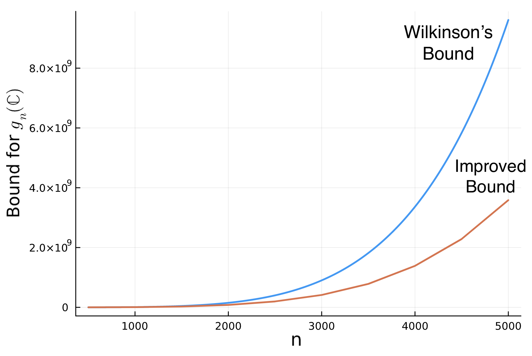
(a) Comparing Wilkinson’s Bound to our Improved Bound for $g_{n}(\mathbb{C})$ for $n\leq 5000$

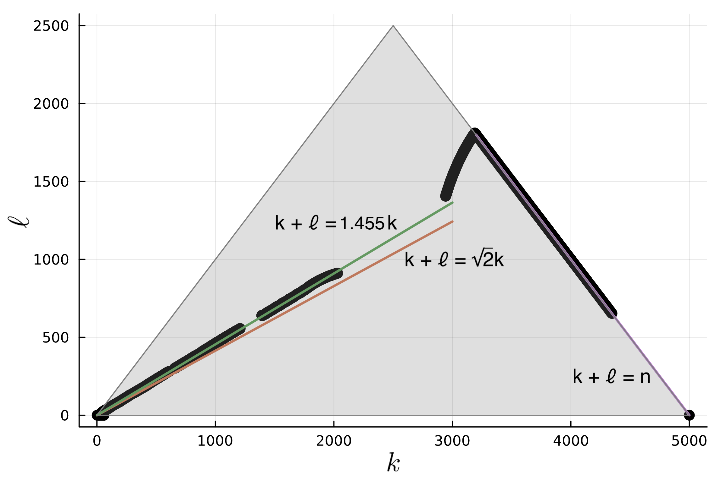
(b) Active constraints parameterized by $(k,\ell)$ for the optimal solution to Program 3.5 at $n=5000$

Figure 1. Comparing our Improved Linear Program to Wilkinson’s LP: Figure (a) illustrates the difference between Wilkinson’s bound for $g_{n}(\mathbb{C})$ (Inequality 1.1) and the upper bound produced by the optimal value of Program 3.5 for $n\leq 5000$. This illustrates that our improved linear program gives superior estimates even for very small $n$. Figure (b) is a scatter plot of the pairs $(k,\ell)$ for which the corresponding inequality in Program 3.5 is tight for a numerically computed optimal solution at $n=5000$. The grey shaded triangle shows the set of $(k,\ell)$ corresponding to constraints of Program 3.5, with Wilkinson’s constraints parameterized by $(k,0)$, and the black dots represent the subset of those constraints that are active for the numerically computed optimal solution. For $n=5000$, almost none of Wilkinson’s constraints are active. The red line $k+\ell=\sqrt{2}k$ is the set of constraints used in Section 4 to prove Theorem 1.1, and the green line denotes the asymptotically tight constraints for the feasible point produced in Subsection 4.1. While the points on the purple line $k+\ell=n$ improves the objective value, these constraints do not play a role in the asymptotic leading term of the solution to the linear program.

Proof.

Let $(q_{1},...,q_{n})$ be a feasible point of Linear Program 3.5. It suffices to show that $p_{k}=k^{3/2}e^{q_{k}}$, $k=1,...,n$, is a feasible point of Optimization Problem 3.3. Considering an arbitrary constraint parameterized by $k>1$ and $\ell$, we have

$$\prod_{i=1}^{k}p_{i}=(k!)^{\tfrac{3}{2}}\exp\bigg{\{}\sum_{i=1}^{k}q_{i}\bigg{\}}\leq(k!)^{\tfrac{3}{2}}\exp\bigg{\{}\frac{k}{2}\ln(\tfrac{11}{4}k)+(k-\ell)q_{k+\ell}+\ell q_{k}\bigg{\}}.$$

Rewriting the right-hand side in terms of $p_{k}$ gives

$$\prod_{i=1}^{k}p_{i} \leq\frac{(k!)^{\tfrac{3}{2}}(\tfrac{11}{4}k)^{\tfrac{k}{2}}p_{k+\ell}^{k-\ell}\,p_{k}^{\ell}}{(k+\ell)^{\tfrac{3}{2}(k-\ell)}k^{\tfrac{3}{2}\ell}}\leq k^{\tfrac{k}{2}}p_{k+\ell}^{k-\ell}\,p_{k}^{\ell}\frac{(k!)^{\tfrac{3}{2}}(\tfrac{11}{4})^{\tfrac{k}{2}}}{k^{\tfrac{3}{2}k}}\leq k^{\tfrac{k}{2}}p_{k+\ell}^{k-\ell}\,p_{k}^{\ell}\leq\frac{k^{k}p_{k+\ell}^{k-\ell}(p_{k}+p_{k+\ell})^{\ell}}{(k-\ell)^{\frac{k-\ell}{2}}\ell^{\frac{\ell}{2}}},$$

completing the proof. ∎

In the following section, we provide nearly matching upper and lower bounds on the optimal value of Program 3.5 for sufficiently large $n$, thereby proving Theorem 1.1.

3.4. Bounding the Growth Factor in Practice

While the proof of Theorem 1.1 focuses on the behavior for large $n$, we note that an improvement in exponential constant exists in practice for reasonably sized matrices as well. We provide a comparison of the optimal value of Program 3.5 to the optimal value of Wilkinson’s LP in Figure 1 for $n\leq 5000$. The numerically computed solutions to Program 3.5 were obtained using the Gurobi Optimizer [10] called through the JuMP package for mathematical optimization [12] in the Julia programming language [1]. We stress that numerically computed solutions to a linear program can be converted into mathematical bounds via a dual feasible point verified in exact arithmetic. In addition, Program 3.5 can be adapted in a number of ways for computational efficiency. For instance, the linear transformation $Q(k)=\sum_{i=1}^{k}q_{i}$ produces a linear program with a simple objective and sparse constraints (at most four variables in each). Furthermore, as the analysis in Section 4 suggests, only a linear number of constraints are required to produce a reasonable upper bound for the optimal value. One natural choice would consist of Wilkinson’s original constraints, and all additional constraints of the form $k+\ell=n$ and $k+\ell\in[\sqrt{2}k-1,\sqrt{2}k+C]$ for some constant $C$ (Theorem 1.1 is proved using only constraints of the form $k+\ell=\lceil\sqrt{2}k\rceil$). Finally, we stress that the techniques used in this paper to produce improved estimates can be further optimized to obtain even better bounds in both theory and practice. We hope that the interested reader will do so.

4. Bounding the Optimal Value of our Linear Program

Finally, we prove that the objective of Program 3.5 satisfies the bound

$$\max\;q_{1}-q_{n}\,\leq\,\alpha\ln^{2}n+(\beta+1/2)\ln n,\qquad\text{where}\quad\alpha=\frac{1}{2(2+(2-\sqrt{2})\ln 2)}$$

and $\beta=0.41$, thus completing the proof of Theorem 1.1. We do so via a duality argument, making use of the constraints for $k$ and $\ell$ satisfying $k+\ell\approx\sqrt{2}k$. Before proving the above bound, we first illustrate why $[2(2+(2-\sqrt{2})\ln 2)]^{-1}$ is the correct choice of $\alpha$ for constraints of the form $k+\ell\approx\sqrt{2}k$, and show that this choice is within $0.00024$ of the exact asymptotic constant of Program 3.5.

4.1. On the Choice and Optimality of the Constant $\alpha=[2(2+(2-\sqrt{2})\ln 2)]^{-1}$

Suppose that $q_{x}-q_{1}=-\gamma\ln^{2}x+O(1)$. Then, for the constraint

$$\sum_{i=1}^{k}(q_{i}-q_{1})\leq\frac{k}{2}\ln(\tfrac{11}{4}k)+(k-\ell)(q_{k+\ell}-q_{1})+\ell(q_{k}-q_{1}),$$

the left-hand side equals

$$\int_{1}^{k}-\gamma\ln^{2}x\;\mathrm{d}x+O(k)=-\gamma k\ln^{2}k+2\gamma k\ln k+O(k)$$

and the right-hand side equals

$$-\gamma k\ln^{2}k+\big{[}k/2-2\gamma(k-\ell)\ln(1+\ell/k)\big{]}\ln k+O(k).$$

Letting $t=\ell/k$, the right-hand side is asymptotically larger than the left-hand side if

$$\gamma\leq\frac{1}{4(1+(1-t)\ln(1+t))}.$$

The values $t=0$ and $t=1$ (e.g., when $\ell=0$ or $\ell=k$) correspond to the constraints of Wilkinson’s linear program, and for $t=0$ and $t=1$, we obtain $\gamma\leq 1/4$ (e.g., Wilkinson’s bound). The value $t=\sqrt{2}-1$ produces the upper bound $1/[2(2+(2-\sqrt{2})\ln 2)]\approx 0.20781$ of Theorem 1.1. The quantity $[4(1+(1-t)\log(1+t))]^{-1}$ on the interval $[0,1]$ is minimized by $t=\exp\{W(2e)-1\}-1\approx 0.4547$, where $W(x)$ is the Lambert W function, with a minimum value of

$$\frac{1}{4\big{(}1+(2-e^{W(2e)-1})(W(2e)-1)\big{)}}\approx 0.207576.$$

This implies the existence of a solution to Program 3.5 with $q_{1}-q_{n}=0.207575\ln^{2}n-O(\ln n)$, thus illustrating that our upper bound of $\alpha=[2(2+(2-\sqrt{2})\ln 2)]^{-1}\approx 0.207811$ is within $0.00024$ of the optimal value of the linear program. We do not pursue further improvement on this constant.

4.2. Reducing Theorem 1.1 to Geometric Mean Growth

For ease of analysis, we consider a continuous version of our variables $q=(q_{1},...,q_{n})$. Let

$$f(x)=q_{\lceil x\rceil}-q_{1}\qquad\text{and}\qquad F(x)=\frac{1}{x}\int_{0}^{x}f(t)\,\mathrm{d}t\qquad\text{for }x>0,$$

where $\{q_{k}\}_{k=1}^{\infty}$ is any sequence such that $(q_{1},...,q_{n})$ is a feasible point of Program 3.5 for all $n\in\mathbb{N}$. Any optimal solution $(q_{1},...,q_{n})$ for the $n$-dimensional linear program can be converted into such a sequence by simply setting $q_{k}=q_{n}$ for all $k>n$. The constraint of Program 3.5 with $k=\lceil x\rceil$ and $\ell=\lceil\sqrt{2}x\rceil-\lceil x\rceil$ implies that for all $x>0$,

$$F(\lceil x\rceil) \leq\frac{\ln(\tfrac{11}{4}\lceil x\rceil)}{2}+\left(\frac{2\lceil x\rceil-\lceil\sqrt{2}x\rceil}{\lceil x\rceil}\right)f(\sqrt{2}x)+\left(\frac{\lceil\sqrt{2}x\rceil-\lceil x\rceil}{\lceil x\rceil}\right)f(x)$$

$$\leq\frac{\ln(\tfrac{11}{4}x)}{2}+\frac{1}{2x}+\left(\sqrt{2}-1-\frac{\sqrt{2}}{x}\right)\left(\sqrt{2}f(\sqrt{2}x)+f(x)\right).$$ (4.1)

We make the following claim regarding $F(x)$.

Lemma 4.1.

$F(x)>-\alpha\ln^{2}x-\beta\ln x$ for all $x>100$.

Lemma 4.1 implies our desired result, as

$$F(n)=\frac{1}{n}\sum_{i=1}^{n}(q_{i}-q_{1})\leq\frac{1}{n}\bigg{(}\frac{n}{2}\ln n+nq_{n}-nq_{1}\bigg{)},$$

and $\alpha\ln^{2}n+(\beta+1/2)\ln n$ is larger than Wilkinson’s bound for $x\leq 100$. A tighter bound may be obtained by adding together constraints of the form $k+\ell=n$ for $k\geq n/(8\alpha)$ (e.g., the constraints appearing in Figure 1(b)). However, the analysis is involved and the improvement on the $1/2\,\ln n$ term produced by the argument above is minor ($\approx 0.046$ improvement, at the cost of lower-order terms).

4.3. Proof of Lemma 4.1: Base Case

The proof of Lemma 4.1 is, in spirit, by “induction on $x$” via a duality argument. Clearly the assertion holds for $x\in(100,1700]$ for $\beta$ sufficiently large. However, verifying the base case of $x\in(100,1700]$ for $\beta=0.41$ requires some analysis, as the quantity $\alpha\ln^{2}n+\beta\ln n$ is strictly less than Wilkinson’s bound. We have

$$F(x)=\frac{1}{x}\int_{0}^{x}q_{\lceil t\rceil}-q_{1}\,\mathrm{d}t=\frac{x-\lfloor x\rfloor}{x}(q_{\lceil x\rceil}-q_{1})+\frac{1}{x}\sum_{k=1}^{\lfloor x\rfloor}(q_{k}-q_{1}).$$

By Inequalities 1.1 and 2.5,

$$q_{1}-q_{\lceil x\rceil}\leq\frac{\ln^{2}\lceil x\rceil}{4}+\frac{\ln\lceil x\rceil}{2}+\ln 2\qquad\text{ and }\qquad\frac{1}{\lfloor x\rfloor}\sum_{k=1}^{\lfloor x\rfloor}(q_{1}-q_{k})\leq\frac{\ln^{2}\lfloor x\rfloor}{4}+\ln 2.$$

Altogether, we obtain the lower bound

$$F(x) \geq-\frac{1}{x}\bigg{(}\frac{\ln^{2}\lceil x\rceil}{4}+\frac{\ln\lceil x\rceil}{2}+\ln 2\bigg{)}-\bigg{(}\frac{\ln^{2}\lfloor x\rfloor}{4}+\ln 2\bigg{)}$$

$$\geq-\frac{1}{x}\bigg{(}\frac{(\ln x+\tfrac{1}{x})^{2}}{4}+\frac{\ln x+\tfrac{1}{x}}{2}+\ln 2\bigg{)}-\bigg{(}\frac{\ln^{2}x}{4}+\ln 2\bigg{)}.$$

By inspection, the right-hand side of the above inequality is strictly greater than $-(\alpha\ln^{2}x+\beta\ln x)$ for our interval of interest $x\in[100,1700]$.

4.4. Proof of Lemma 4.1: Inductive Step

In order to verify the claim for some $y>1700$, we integrate over $x\in\big{[}\tfrac{y}{2},\tfrac{y}{\sqrt{2}}\big{]}$ to obtain a lower bound for $F(y)$ in terms of $F(x)$ for $x<y$. In particular, by integrating Inequality 4.1 over $x\in\big{[}\tfrac{y}{2},\tfrac{y}{\sqrt{2}}\big{]}$ we have

$$\frac{1}{\frac{y}{\sqrt{2}}-\frac{y}{2}}\int_{\frac{y}{2}}^{\frac{y}{\sqrt{2}}}F(\lceil x\rceil)\,\mathrm{d}x\, \leq\,\frac{1}{\frac{y}{\sqrt{2}}-\frac{y}{2}}\left[\bigg{(}\sqrt{2}-1-\frac{2\sqrt{2}}{y}\bigg{)}\int_{\frac{y}{2}}^{y}f(x)\,\mathrm{d}x+\int_{\frac{y}{2}}^{\frac{y}{\sqrt{2}}}\frac{\ln(\tfrac{11}{4}x)}{2}+\frac{1}{2x}\,\mathrm{d}x\right]$$

$$=\,\bigg{(}1-\frac{4+2\sqrt{2}}{y}\bigg{)}\big{(}2F(y)-F(\tfrac{y}{2})\big{)}+\frac{\ln y}{2}$$

$$\qquad+\frac{\ln 2+\sqrt{2}\ln\tfrac{11}{4}-\sqrt{2}}{2\sqrt{2}}+\frac{(\sqrt{2}+1)\ln 2}{2y}.$$

Rearranging the above inequality allows us to lower bound $F(y)$ by a positive linear combination of $F(x)$ for $x\in\big{[}\tfrac{y}{2},\tfrac{y}{\sqrt{2}}\big{]}$. We note that this is the reason for the choice of $k+\ell\approx\sqrt{2}k$, as this approach does not give us such a bound if $\sqrt{2}$ is replaced by a larger constant. Now, suppose our claim is false, and let $y>1700$ be the smallest value such that $F(y)\leq-\alpha\ln^{2}y-\beta\ln y$. We aim to show that this contradicts the above lower bound for $F(y)$. By assumption,

$$F(\lceil x\rceil) >-\alpha\ln^{2}(x+1)-\beta\ln(x+1)$$

$$>-\alpha\ln^{2}x-\beta\ln x-\frac{2\alpha\ln x}{x}-\frac{\beta}{x}-\frac{\alpha}{x^{2}}\qquad\text{for }x\in\big{[}\tfrac{y}{2},\tfrac{y}{\sqrt{2}}\big{]},$$

implying that

$$\frac{1}{\frac{y}{\sqrt{2}}-\frac{y}{2}}\int_{\frac{y}{2}}^{\frac{y}{\sqrt{2}}}F(\lceil x\rceil)\,\mathrm{d}x\, >\,-\alpha\ln^{2}y-\big{(}(\sqrt{2}\ln 2-2)\alpha+\beta\big{)}\ln y-\bigg{(}\frac{\ln 2}{\sqrt{2}}-1\bigg{)}\beta$$

$$\qquad-\bigg{(}2-\frac{(3+\sqrt{2})\ln^{2}2}{2\sqrt{2}}-\sqrt{2}\ln 2\bigg{)}\alpha-\frac{2(\sqrt{2}+1)\alpha\ln 2\ln y}{y}$$

$$\qquad\qquad-\frac{(\sqrt{2}+1)(\beta\ln 2-\tfrac{3}{2}\alpha\ln^{2}2)}{y}-\frac{2\sqrt{2}\alpha}{y^{2}}.$$

In addition,

$$2F(y)-F(\tfrac{y}{2})<-\alpha\ln^{2}y-(2\alpha\ln 2+\beta)\ln y+\alpha\ln^{2}2-\beta\ln 2.$$

Combining our upper and lower bounds, we observe that the terms containing $\ln^{2}y$ are equal, and the terms containing $\ln y$ are equal

$$-\big{(}(\sqrt{2}\ln 2-2)\alpha+\beta\big{)}=\frac{1}{2}-(2\alpha\ln 2+\beta)$$

due to the value of $\alpha$. We are left with the inequality

$$\frac{(\sqrt{2}-1)\ln 2+\sqrt{2}}{\sqrt{2}}\beta+\frac{(2-\sqrt{2})\ln^{2}2-4(2-\sqrt{2})(\ln\frac{11}{4}-1)\ln 2-8\ln\frac{11}{4}}{8(2+(2-\sqrt{2})\ln 2)}+g(\beta,y)<0,$$

where $g(\beta,y)$ is a linear function of $\beta$ of order $O(\ln^{2}(y)/y)$. The left-hand side is strictly greater than zero for a sufficiently large choice of $\beta$. However, verifying that our choice of $\beta=0.41$ is sufficiently large requires an explicit analysis of $g(\beta,y)$ for $\beta=0.41$ and $y>1700$. The function $g(\beta,y)$ is given by

$$g(\beta,y) =-\frac{2+\sqrt{2}}{2+(2-\sqrt{2})\ln 2}\,\frac{\ln^{2}y}{y}-\bigg{(}(4+2\sqrt{2})\beta+\frac{(5+3\sqrt{2})\ln 2}{2+(2-\sqrt{2})\ln 2}\bigg{)}\,\frac{\ln y}{y}$$

$$\qquad+\bigg{(}\frac{(11+4\sqrt{2})\ln^{2}2}{4(2+(2-\sqrt{2})\ln 2)}-(5+3\sqrt{2})\beta\ln 2-\frac{(\sqrt{2}+1)\ln 2}{2}\bigg{)}\,\frac{1}{y}$$

$$\qquad\qquad-\frac{\sqrt{2}}{2+(2-\sqrt{2})\ln 2}\,\frac{1}{y^{2}}.$$

When $\beta=0.41$ and $y>1700$,

$$\frac{(\sqrt{2}-1)\ln 2+\sqrt{2}}{\sqrt{2}}\beta+\frac{(2-\sqrt{2})\ln^{2}2-4(2-\sqrt{2})(\ln\frac{11}{4}-1)\ln 2-8\ln\frac{11}{4}}{8(2+(2-\sqrt{2})\ln 2)}>0.086$$

and

$$g(0.41,y)>-\frac{\tfrac{3}{2}\ln^{2}y}{y}-\frac{6\ln y}{y}-\frac{3}{y}-\frac{1}{y^{2}}>-\frac{\tfrac{3}{2}\ln^{2}1700}{1700}-\frac{6\ln 1700}{1700}-\frac{3}{1700}-\frac{1}{1700^{2}}>-0.08,$$

thus obtaining our desired contradiction. This completes the proof of Theorem 1.1.

References

- [1] Jeff Bezanson, Alan Edelman, Stefan Karpinski, and Viral B Shah. Julia: A fresh approach to numerical computing. SIAM review, 59(1):65–98, 2017.
- [2] Rajendra Bhatia. Matrix analysis, volume 169. Springer Science & Business Media, 2013.
- [3] AM Cohen. A note on pivot size in Gaussian elimination. Linear Algebra and its Applications, 8(4):361–368, 1974.
- [4] Colin W Cryer. Pivot size in Gaussian elimination. Numerische Mathematik, 12(4):335–345, 1968.
- [5] Alan Edelman. The complete pivoting conjecture for Gaussian elimination is false. 1992.
- [6] Alan Edelman and John Urschel. Some new results on the maximum growth factor in Gaussian elimination. arXiv preprint arXiv:2303.04892, 2023.
- [7] Herman H Goldstine. The computer from Pascal to von Neumann. Princeton University Press, 1993.
- [8] Gene H Golub and Charles F Van Loan. Matrix computations. JHU press, 2013.
- [9] Nick Gould. On growth in Gaussian elimination with complete pivoting. SIAM Journal on Matrix Analysis and Applications, 12(2):354–361, 1991.
- [10] Gurobi Optimization, LLC. Gurobi Optimizer Reference Manual, 2023.
- [11] Chi-Kwong Li and Roy Mathias. The determinant of the sum of two matrices. Bulletin of the Australian Mathematical Society, 52(3):425–429, 1995.
- [12] Miles Lubin, Oscar Dowson, Joaquim Dias Garcia, Joey Huchette, Benoît Legat, and Juan Pablo Vielma. JuMP 1.0: Recent improvements to a modeling language for mathematical optimization. Mathematical Programming Computation, 2023.
- [13] Carl Meyer. History of Gaussian elimination. http://carlmeyer.com/pdfFiles/GaussianEliminationHistory.pdf.
- [14] Erich Strohmaier, Jack Dongarra, Horst Simon, and Martin Meuer. Top 500 list: November 2023. https://www.top500.org/lists/top500/2023/11/.
- [15] Leonard Tornheim. Pivot size in Gauss reduction. Tech Report, Chevron Research Co., Richmond CA, 1964.
- [16] Leonard Tornheim. Maximum third pivot for Gaussian reduction. In Tech. Report. Calif. Res. Corp Richmond, Calif, 1965.
- [17] Leonard Tornheim. A bound for the fifth pivot in Gaussian elimination. Tech Report, Chevron Research Co., Richmond CA, 1969.
- [18] Leonard Tornheim. Maximum pivot size in Gaussian elimination with complete pivoting. Tech Report, Chevron Research Co., Richmond CA, 10, 1970.
- [19] John von Neumann and Herman H Goldstine. Numerical inverting of matrices of high order. 1947.
- [20] James Hardy Wilkinson. Error analysis of direct methods of matrix inversion. Journal of the ACM (JACM), 8(3):281–330, 1961.