Probing Correlations in the Binary Black Hole Population with Flexible Models

Abstract

The astrophysical formation channels of binary black hole systems predict correlations between their mass, spin, and redshift distributions, which can be probed with gravitational-wave observations. Population-level analysis of the latest LIGO-Virgo-KAGRA catalog of binary black hole mergers has identified evidence for such correlations assuming linear evolution of the mean and width of the effective spin distribution as a function of the binary mass ratio and merger redshift. However, the complex astrophysical processes at play in compact binary formation do not necessarily predict linear relationships between the distributions of these parameters. In this work, we relax the assumption of linearity and instead search for correlations using a more flexible cubic spline model. Our results suggest a nonlinear correlation between the width of the effective spin distribution and redshift. We also show that the LIGO-Virgo-Kagra collaborations may find convincing Bayesian evidence for nonlinear correlations by the end of the fourth observing run, O4. This highlights the valuable role of flexible models in population analyses of compact-object binaries in the era of growing catalogs.

I Introduction

The growing catalog of gravitational-wave observations of binary black hole (BBH) mergers has allowed for increasingly detailed probes of the population properties of these systems, with the ultimate goal of revealing how they form and evolve. Analysis of the third gravitational-wave transient catalog (GWTC-3) [1] of the LIGO-Virgo-Kagra collaboration (LVK) [2, 3, 4, 5, 6] found evidence for substructure in the BBH primary mass distribution [7, 8, 9] beyond a single power-law [10] plus Gaussian peak [11] and for preferentially equal-mass mergers [12, 13]. The black hole spin distribution favors small [14] but likely nonzero spins [15, 16, 17, 18, 19, 20], and the distribution of the spin tilts relative to the orbital angular momentum is consistent with isotropy [20, 7, 21]. The merger rate evolves with redshift at a rate consistent with the cosmic star formation rate [22]. Taken altogether, these constraints imply that there are probably multiple formation channels [23, 24, 25] shaping the BBH population, although no definitive evidence for sub-populations with different properties has been identified [26, 27, 28].

While most previous analyses of the BBH population have relied on phenomenological population models with simple parametric functional forms, recent work has explored the use of “non-parametric” models like splines [29, 30], Dirichlet processes [31], generic mixture models [8, 32, 33], and autoregressive models [34]. Despite including many more free parameters than the phenomenological models, these non-parametric models offer increased flexibility to fit the data without imposing a specific functional form. This avoids the issue of model misspecification [e.g., 35] at the cost of a clear mapping between features observed in the data and those predicted by astrophysical theory.

As the observed population of BBH mergers grows, population analyses have moved beyond modeling the mass, spin, and redshift distributions independently towards searching for correlations between these parameters. Such correlations are expected both within individual formation channels and due to the superposition of sub-populations forming via distinct channels [36, 37, 38, 39, 40, 41, 42, 43]. For example, BBHs formed via isolated binary evolution may exhibit correlations due to the relationship between metallicity and the efficiency of angular momentum transport via stellar winds, which remove mass and spin down the progenitor, meaning that more massive systems would preferentially have high spins and be found at high redshift where stellar winds are less efficient because of lower metallicities [44]. A mass-spin correlation is also expected for systems formed dynamically via hierarchical mergers in dense environments, since remnants of previous mergers that go on to merge again will be both more massive and rapidly spinning [e.g., 45, 46, 47].

Evidence for a correlation between BBH mass and spin was obtained using a phenomenological model where the mean and width of the distribution of effective aligned spin ($\chi_{\rm eff}$) vary linearly as a function of the mass ratio, such that systems with more unequal mass ratios have larger effective aligned spins [48, 7]. An approach using copula density functions that ensure fixed marginal distributions in the presence of a correlation identifies this correlation at similar significance [49, 50]. Weaker evidence using the linear correlation model also hints at a potential correlation between the effective spin distribution and the total mass and primary mass [51, 52, 53], although a broadening of the spin distribution at the highest masses can be explained due to the relative dearth of observations in this regime, leading to a more uncertain measurement [33]. A likely correlation between the width of the effective spin distribution and redshift has also been identified [53]. Recently, using a non-parametric method, Ref. [54] reports a correlation in primary mass-redshift space, arising from two sub-populations. However, some results of this work are in tension with previous population analyses, including both parametric and nonparametric methods [e.g. 55, 33, 29, 34].

In this work, we build upon previous methods looking for correlations between individual pairs of parameters describing the BBH mass, spin, and redshift distributions but adopt a more flexible model for the shape of the correlation. Specifically, we assume the BBH effective spin distribution is described by a Gaussian with an unknown mean and width, both of which may correlate with either the mass or redshift such that the shape of the correlation is given by a cubic spline. Our model recovers evidence for the previously-identified correlations between effective spin and mass ratio and redshift but prefers a nonlinear shape for the spin-redshift correlation. This result highlights the important role that flexible population models will play in identifying model misspecification as the catalog of BBH merger observations grows. The rest of this work is structured as follows.

In §II we briefly describe our statistical assumptions, which are standard in gravitational wave (GW) population inference, then describe our model for probing correlations in more detail. In §III we present the constraints on the BBH data collected thus far [1], which tend to be broadly consistent with previous studies apart from some evidence for nonlinearity in the $\chi_{\rm eff}-z$ correlation. In §IV we make projections for the future: how well can nonlinearity be measured with future observations? In a pair of simulated Universes with nonlinear correlations in $\chi_{\rm eff}-q$ and $\chi_{\rm eff}-z$, nonlinearity does not reveal itself in the $\chi_{\rm eff}-q$ distribution with 400 detections, but there is strong evidence for nonlinearity in the $\chi_{\rm eff}-z$ distribution with 400 detections. While the detectability of nonlinearity ultimately is subject to how nonlinear the true correlated distribution is, we show it is possible to detect nonlinearity in the near future. Finally, we conclude in §V.

II Probing Correlations: Priors and Parameterization

The goal of population modeling is to infer the distribution from which an ensemble of observations is drawn. This can be accomplished using hierarchical Bayesian inference, which takes a multi-stage approach by first characterizing individual observations and then combining them on a population level. In a GW context, these individual observations are noisy, so the statistical likelihood of observing the data given a population model $p(\theta|\Lambda)$ parameterized by $\Lambda$ must be marginalized over the possible GW parameters [56]

$$\mathcal{L}(d|\Lambda)=\int{\rm d}\theta\mathcal{L}(d|\theta)p(\theta|\Lambda).$$ (1)

Here, $d$ represents the detected data, and $\theta$ represents the unknown source parameters, like the binary masses, spins, and redshift.

Furthermore, BBHs suffer a Malmquist bias; they are not all equally detectable. To account for this bias, we must define the detection efficiency

$$\alpha(\Lambda)=\int_{\mathcal{D}_{\uparrow}}{\rm d}d\int{\rm d}\theta\mathcal{L}(d|\theta)p(\theta|\Lambda),$$ (2)

which is the fraction of events in the population $p(\theta|\Lambda)$ which probabilistically generate detectable data ($d\in\mathcal{D}_{\uparrow}$). Assuming the events are distributed in time by a Poisson process and marginalizing over the Poisson rate parameter with a uniform-in-$\log$ prior, we obtain the rate-marginalized hierarchical likelihood [56, 57, 58, 59, 60, 61]. In particular, with a collection of $N_{\rm obs}$ events with data $\{d_{i}\}_{i=1}^{N_{\rm obs}}$ passing a detection threshold

$$\mathcal{L}(\{d_{i}\}_{i=1}^{N_{\rm obs}}|\Lambda)\propto\prod_{i=1}^{N_{\rm obs}}\frac{\mathcal{L}(d_{i}|\Lambda)}{\alpha(\Lambda)}.$$ (3)

We use this likelihood to sample from the hyperparameters $\Lambda$. In practice, we estimate the marginal integrals in Eqs. 1 and 2 with Monte Carlo estimators, see Refs. [62, 63, 64] for details.

A common approach tackles the hierarchical inference problem by phenomenologically parameterizing the unknown source distribution as e.g. power-laws, Gaussians, etc., and inferring these hyperparameters given the data observations. Previous studies have identified simple and successful parameterization schemes; we choose the astrophysically motivated parameterizations Power-Law + Peak [11] and Power-Law Redshift [65] for the mass $p(m_{1},q|\Lambda)$ and redshift $p(z|\Lambda)$ distributions respectively. The primary mass distribution is parameterized as a smoothed power-law plus a gaussian component, and a smoothed power-law for the mass ratio (hyperparameters are the minimum and maximum BH mass–assumed to be the same for both the primary and secondary–power-law index, low mass smoothing parameter, mean and width of the Gaussian, fraction of BBHs in the Gaussian component, and the power-law index for the mass ratio). The redshift distribution is modelled as a power-law with a single power-law index hyperparameter.

For the spins, we project the 6 dimensional spin distribution to a one dimensional parameter $\chi_{\rm eff}$ describing the leading order spin effect on the inspiral evolution of the binary [66, 67, 68], which is often the most well measured spin parameter [69, 70]. We then model the $\chi_{\rm eff}$ population as a truncated Gaussian distribution with a variable mean and width [71, 72]

$$p(\chi_{\rm eff}|\theta,\Lambda)=\frac{1}{\sigma(\theta,\Lambda)}\frac{\phi\left(\frac{\chi_{\rm eff}-\mu(\theta,\Lambda)}{\sigma(\theta,\Lambda)}\right)}{\Phi\left(\frac{1-\mu(\theta,\Lambda)}{\sigma(\theta,\Lambda)}\right)-\Phi\left(\frac{-1-\mu(\theta,\Lambda)}{\sigma(\theta,\Lambda)}\right)}$$ (4)

where the truncation restricts the support of the distribution to be $[-1,1]$, which reflects the physical constraint that the magnitude of $\chi_{\rm eff}$ cannot exceed 1 for BH spins bounded by the Kerr limit. $\phi$ is the standard Gaussian and $\Phi$ is the standard error function,

$$\phi(x)=\frac{e^{-x^{2}/2}}{\sqrt{2\pi}}\qquad\Phi(x)=\int_{-\infty}^{x}\phi(s)ds.$$ (5)

This is the approach used by Refs. [7, 51, 48, 53] to explore models where $\mu(\theta)$ and $\sigma(\theta)$ are linear functions of primary mass ($\theta=m_{1}$) mass ratio ($\theta=q$) and redshift ($\theta=z$) respectively. Building on this previous work, we model $\mu(\theta)$ and $\sigma(\theta)$ with spline functions.

Spline functions are becoming increasingly popular in GW population inference, primarily because they are innately flexible and fast to evaluate, but also because they are easily parameterized by their nodes. While splines do not assume much structure, they do fail to probe structure below the scale of the node separation length. For this reason, one should include the number of nodes as a model hyperparameter or repeat the analysis varying the choice of the number of nodes.

In this work, we use a cubic spline model, where nodes are interpolated using cubic polynomials which preserve continuity in the function and first and second derivatives at the nodes ($\mathcal{C}^{2}$ functions). Given node locations, this provides all but two conditions to set the four coefficients for each cubic polynomial; the final two conditions are given at the endpoints, typically imposed by setting the second derivative to zero. Defined in this way, the node positions fully determine the spline curve. Splines also have the advantage of approximate locality, meaning they can fit a structure in one region of parameter space independently of the behavior of the spline far away (separated by many nodes) [73].

For all the inferences we present below, we use priors shown in Table 1. We use the Overall samples for GWTC1 events [74], PrecessingSpinIMRHM for the events first identified in GWTC2 [75] and the C01:IMRPhenomXPHM samples for the GWTC2.1 and GWTC3 events [76, 77], and the search sensitivity estimates provided in Ref. [78]. We use the GWPopulation package for constructing the hierarchical likelihood [79], and compute Bayesian evidences while sampling the hyperposterior using the Dynesty implementation in Bilby [80, 81]. To efficiently evaluate spline functions, we use the cached_interpolate package introduced in Ref. [30]. In addition, because we estimate the population likelihood (Eq. 3) with Monte Carlo integrals, there is inherent uncertainty associated with each likelihood estimate. To avoid biased inference, we cut hyperposterior samples with $\log$-likelihood uncertainty greater than 1, following the recommendation of Ref. [64].

Hyperparameter	Description	Prior
$\alpha$	$m_{1}$ power-law index	U(-4, 12)
$\beta$	$q$ power-law index	U(-4, 7)
$m_{\rm max}$	maximum BH mass	U$(60\;M_{\odot},100\;M_{\odot})$
$m_{\rm min}$	minimum BH mass	U$(2\;M_{\odot},10\;M_{\odot})$
$\delta_{m}$	low-mass smoothing parameter	U$(0\;M_{\odot},10\;M_{\odot})$
$\mu_{m}$	$m_{1}$ Gaussian component mean	U$(20\;M_{\odot},50\;M_{\odot})$
$\sigma_{m}$	$m_{1}$ Gaussian component standard deviation	U$(1\;M_{\odot},10\;M_{\odot})$
$\lambda$	fraction of BBHs in Gaussian component	U(0, 0.2)
$\lambda_{z}$	$z$ power-law index	U(-2, 10)
$\mu_{\chi_{\rm eff}:n}$	$n^{\rm th}$ spline node for the $\chi_{\rm eff}$ mean	U$(-1,1)$
$\ln\sigma_{\chi_{\rm eff}:n}$	$n^{\rm th}$ spline node for the $\chi_{\rm eff}$ standard deviation	U$(-5,0)$

Table 1: Priors for each hyperparameter used in our model. The upper panel describes the standard priors, except where they are reduced to improve the sampling efficiency without cutting off the hyperposterior ($m_{\rm max}$ and $\lambda$). The lower panel describes the prior assumed for our spline parameters.

III Correlations in GWTC-3

Using the catalog of 69 BBHs described in Ref. [7] passing a detection-pipeline-computed false alarm rate threshold of 1 yr^-1, we search for evidence of nonlinear correlations between the spin distribution and the mass ratio, redshift, and the source frame primary mass (the latter is described in appendix § VII.1). To do this, we model the $\chi_{\rm eff}$ distribution with Eq. 4, and present the results of the individual analyses below.

III.1 Effective Spin Distribution and Mass Ratio

The first correlation we explore is between $\chi_{\rm eff}$ and mass ratio $q$, setting the mean and standard deviations to spline functions of mass ratio. We place the nodes uniformly between $q=0$ and $q=1$ ,

$$\mu(\theta) =S\left(q\;|\;(0,\mu_{\chi_{\rm eff}:0}),...,(1,\mu_{\chi_{\rm eff}:N})\right)$$

$$\ln\sigma(\theta) =S\left(q\,|\,(0,\ln\sigma_{\chi_{\rm eff}:0}),...,(1,\ln\sigma_{\chi_{\rm eff}:N})\right),$$ (6)

where $S(x\;|\;(X_{1},Y_{1}),...,(X_{N},Y_{N}))$ represents the cubic spline function in the variable $x$ passing through the nodes with $x$ coordinates $X_{1}<X_{2}<...<X_{N}$ and corresponding $y$ coordinates $Y_{1},Y_{2},...,Y_{N}$. In all our models, we fix the $x$ coordinates to reduce the dimension of the inference.

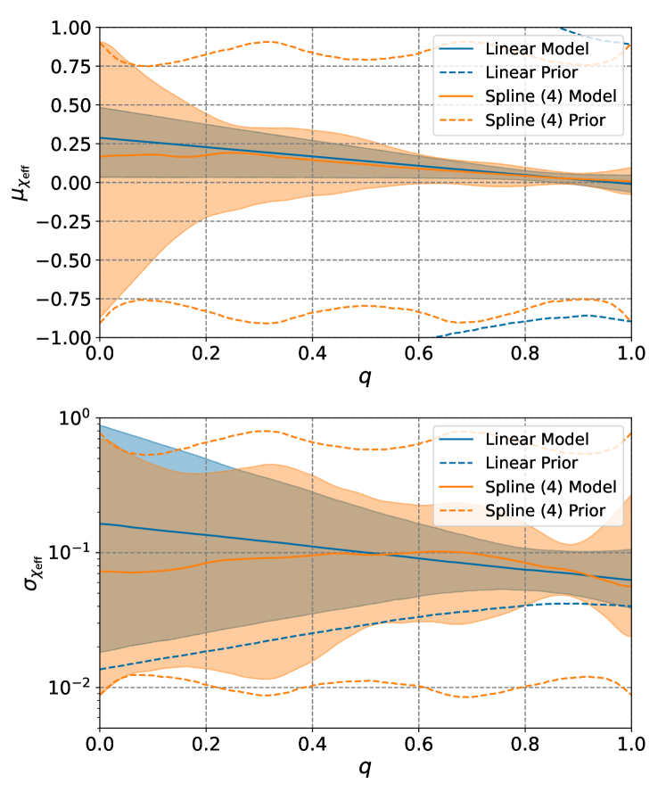
Figure 1: A comparison between the linear model and 4 node spline model for correlation between $\chi_{\rm eff}$ and mass ratio, inferred using GWTC-3. Solid lines represent the median, while the shaded region represents the central 90% credible interval. Dashed lines show the upper and lower boundaries of the prior 90% interval. The upper panel shows the mean of the $\chi_{\rm eff}$ Gaussian as a function of mass ratio $q$, while the lower panel is the standard deviation of the $\chi_{\rm eff}$ distribution.

In Fig. 1, we show a comparison between our results with the linear model of Ref. [48] to the spline model with 4 nodes. While our spline model results are broadly consistent with the linear model, they generically feature broader credible intervals towards extreme mass ratios $q\to 0$. We argue that this is an advantage of the spline model, as the data should have less information about BBHs with unequal mass ratios as they are less common in the detected population [e.g., 12, 13] and be completely uninformative about events with mass ratio $q\to 0$. All of the 69 BBHs in the catalog are inconsistent with vanishing mass ratios, and what’s more, our population model with hyperparameter $m_{\rm min}\geq 2\;M_{\odot}$ (the minimum BH mass must exceed $2\;M_{\odot}$, see Ref. [11]) requires zero support at $q\to 0$. Being an approximately local model, the spline model can fit the structure at near-equal mass ratios, while simultaneously saying nothing about the behaviour of extreme mass ratio events. Hence, the posterior approaches the prior as $q\to 0$. We also repeat the analysis with 3-6 nodes and obtain results consistent with the 4-node analysis presented here, see appendix §VII.2.

To compute the significance of any evolution with mass ratio, we compute the derivative of the inferred evolution with respect to mass ratio. Spline functions are easily differentiable, and so we can compute the slope of the spline function at an arbitrary point $q^{*}$. We choose the fiducial value of $q^{*}=0.9$, as this appears to be a well constrained region and a good proxy for understanding the evolution of the spin population in the region of near-equal mass ratios. This gives us posteriors on the slope at this point $q^{*}$ for each model, which we show in Fig. 2. We then compute the significance of an evolution in the mean of the Gaussian as a function of mass ratio from the fraction of the posterior support with positive/negative slope. The linear model has a negative slope with significance $\sim 98\%$, as initially reported in Ref. [48]. The spline models has negative slope with more inconclusive significance: $\sim 70-80\%$. We show all calculated slope significances at their fiducial values in Table 3 in appendix §VII.2.

Figure 2: Posteriors on the derivative of the mean and width of the $\chi_{\rm eff}$ distribution as a function of mass ratio, calculated at $q^{*}=0.9$, and inferred using GWTC 3. The linear model concludes that the mean of the $\chi_{\rm eff}$ distribution decreases as mass ratio approaches $1$, with a significance of $\sim 98\%$. The spline models are more agnostic, finding significances of $\sim 60-75\%$.

III.2 Effective Spin Distribution and Redshift

Next, we turn our attention to the correlation between $\chi_{\rm eff}$ and redshift $z$. Ref. [53] examined a correlation between redshift and the effective spin distribution, and discovered evidence for a broadening in the effective spin distribution, a positive correlation between the width $\sigma(z)$ of the $\chi_{\rm eff}$ Gaussian and the redshift, and no evidence for any trend in the mean of the Gaussian. In their analysis, Ref. [53] parameterized $\mu(z)=\mu_{0}+\delta\mu_{z}(z-0.5)$ and $\log_{10}\sigma(z)=\log\sigma_{0}+\delta\log\sigma_{z}(z-0.5)$ as linear models and quantified the significance of the measured broadening using the posterior on the slope $\delta\log\sigma_{z}$.

In a similar approach, we model the $\chi_{\rm eff}$ correlation with redshift using Eq. 4, only we use

$$\mu(\theta) =S\left(z\;|\;(0,\mu_{\chi_{\rm eff}:0}),...,(2.3,\mu_{\chi_{\rm eff}:N})\right)$$

$$\ln\sigma(\theta) =S\left(z\;|\;(0,\ln\sigma_{\chi_{\rm eff}:0}),...,(2.3,\ln\sigma_{\chi_{\rm eff}:N})\right).$$ (7)

In our model, the first and last nodes are placed at redshifts $z=0$ and $z=2.3$, the maximum redshift we assume in the Power-Law Redshift model . The hyperparameters associated to the splines are the $y$ coordinates of the nodes. We explored models that fix the nodes uniformly between the first and last nodes; however, these resulted in nodes too coarsely spread at small redshift to optimally fit the structure. Additionally, there is limited information in the data thus far to constrain the population much beyond redshift $z\gtrsim 1$, so a better node spacing should place nodes tightly at small redshift and more loosely at high redshift. Heuristically, we found that a linear spacing in $z^{1/2}$ places nodes satisfactorily.

Using these models to infer the BBH population hyperparameters given the GWTC-3 dataset, we infer the evolution of the mean and width of the $\chi_{\rm eff}$ Gaussian as a function of redshift. We show a comparison between a linear model and the spline model with 4 nodes in Fig. 3. We show the results for a collection of analyses with 3-6 spline nodes in appendix §VII.2 in Fig. 10 and the associated model evidences in Fig. 9.

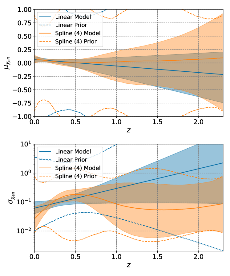
Figure 3: A comparison between the linear model and 4 node spline model for correlation between $\chi_{\rm eff}$ and redshift, inferred using GWTC-3. Solid lines represent the median, while the shaded region represents the central 90% credible interval, and the dashed lines show the boundary of the prior 90% interval. The upper panel shows the mean of the $\chi_{\rm eff}$ Gaussian as a function of redshift $z$, while the lower panel represents the standard deviation of the $\chi_{\rm eff}$ distribution.

First, we quantify the confidence of a broadening slope for each model. To this end, we compute the slope of the width of the Gaussian at a fiducial value $z^{*}$, $\partial\log\sigma(z){z=z^{*}}$ for all models. We choose the fiducial value $z^{*}=0.2$ (see appendix §VII.3 for a discussion on this choice), and show histograms of the slopes for each model in appendix §VII.3 in Fig. 11. We can then quantify the significance of the increase by the proportion of the posterior with slope greater than zero.

There are varying degrees of evidence that the $\chi_{\rm eff}$ distribution is broadening as a function of redshift at $z^{*}=0.2$, depending on the model used. The mean is decreasing at $\sim 80-95\%$ confidence (the posterior support with slope less than 0), depending on the model assumed. The width is increasing at $90-98.6\%$ confidence, consistent with the finding of Ref. [53] that the width of the $\chi_{\rm eff}$ distribution broadens with increasing redshift. We collect all significances calculated at fiducial values in Table 3 in appendix §VII.2.

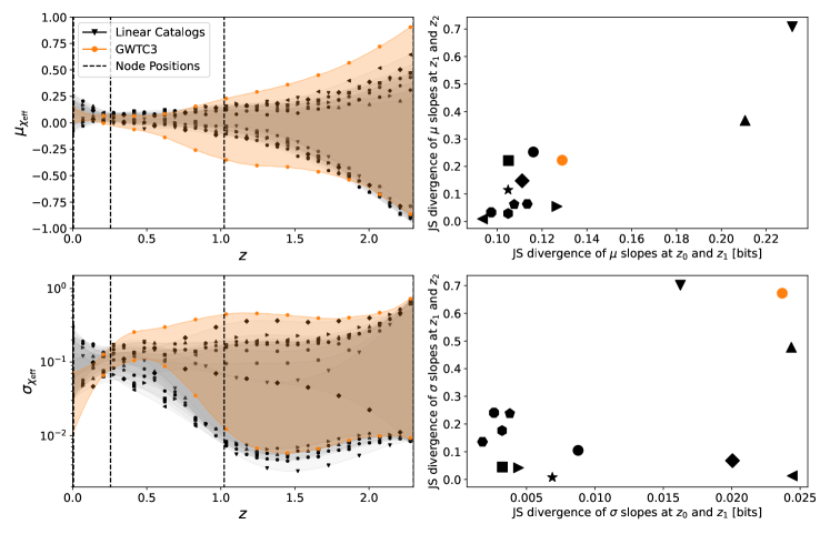
Figure 4: Comparison between the spline inference on a linearly correlated Universe and the inference on GWTC-3. The first row shows the mean and the second row the standard deviation. The left column shows the 90% credible intervals inferred using GWTC-3 (orange) and the 12 synthetic catalogs of 69 events drawn from a linearly correlated Universe (gray). The right column shows the Jensen-Shannon (JS) divergences (in bits) between slope posteriors taken at the first two nodes on the x-axis, and between the second and third nodes on the y-axis. For each linear catalog there is a black point on the scatter plot, and the orange point corresponds to the GWTC-3 divergences. This represents the posterior difference between the two slopes, quantifying the nonlinearity. The further the point is from the origin, the more confident we are in the inferred nonlinearity. Notice there is no inference on a linear Universe which is more nonlinear than GWTC-3 in both dimensions.

It also appears that there is some nonlinearity in the evolution of the width as a function of redshift. To understand if this degree of inferred nonlinearity is expected in a Universe with a linear correlation, we perform the spline model inference with 4 nodes on 12 catalogs of 69 events drawn from a linearly correlated Universe, (see appendix §VII.3 for details on the selection procedure and the generation of the synthetic catalogs). We then compute the derivative at the first three nodes $z_{0}$, $z_{1}$ and $z_{2}$ (ignoring the last node since the posterior is essentially the prior there) and calculate the Jensen-Shannon (JS) divergence [84, 85] between the slope posteriors. A linearly correlated Universe would theoretically have slope posteriors all consistent with the true value, however there will be some random scatter between the posteriors, measured by the JS divergence between them. Looking at a scatter plot of the divergence between the slope at $z_{0}$ and $z_{1}$ on the x-axis and between $z_{1}$ and $z_{2}$ on the y-axis in Fig. 4, notice that there are no divergences from a linearly correlated Universe which is more extreme than the GWTC-3 divergences in both axes. This points towards a nonlinear trend in the width of the $\chi_{\rm eff}$ distribution as a function of redshift, though the Bayesian evidence ($\mathcal{Z}=\int\pi(\Lambda)\mathcal{L}(\{d_{i}\}|\Lambda)d\Lambda$) is not yet conclusive (see Fig. 9 in appendix §VII.2)

IV Future Prospects: Can We Detect Nonlinearity in O4?

Flexible spline models stand in contrast to linear models, where the correlation around each spline node is independently inferred, rather than enforcing a consistent slope across the whole parameter space. At the conclusion of O3, these flexible models highlight our lack of knowledge about poorly constrained regions. While we have some hints of a nonlinear correlation in $\chi_{\rm eff}-z$, there is not yet a definitive preference in the Bayesian evidence for a nonlinear correlation. This may change by the end of the fourth observing run, O4.

To predict how well we may actually detect nonlinear correlations in the future, we produced two synthetic catalogs of 200 events and 400 events for two different possible Universes (so four catalogs total). The events are detected by a network of LIGO interferometers (located at Hanford and Livingston), assuming the fiducial O4 noise spectra with an average BNS inspiral range of 160 Mpc [86]. We draw GW events from a few different populations with true hyperparameters given in Table 2. These populations are consistent with the data collected by the LVK thus far, analyzed with the models we presented above. We use the waveform model IMRPhenomXP with PrecVersion=104 [87], and use the heterodyning/relative binning scheme of Refs. [88, 89, 90] to efficiently sample the GW event parameter posteriors.

Hyperparameter	Description	$q-\chi_{\rm eff}$ Correlation	$z-\chi_{\rm eff}$ Correlation
$\alpha$	$m_{1}$ power-law index	$3$	$3$
$\beta$	$q$ power-law index	1	1
$m_{\rm max}$	maximum BH mass	$85\;M_{\odot}$	$85\;M_{\odot}$
$m_{\rm min}$	minimum BH mass	$5\;M_{\odot}$	$5\;M_{\odot}$
$\delta_{m}$	low-mass smoothing parameter	$3\;M_{\odot}$	$3\;M_{\odot}$
$\mu_{m}$	$m_{1}$ Gaussian component mean	$35\;M_{\odot}$	$35\;M_{\odot}$
$\sigma_{m}$	$m_{1}$ Gaussian component standard deviation	$5\;M_{\odot}$	$5\;M_{\odot}$
$\lambda$	fraction of BBHs in Gaussian component	$0.03$	$0.03$
$\lambda_{z}$	$z$ power-law index	2	2
$(x_{0},\mu_{\chi_{\rm eff}:0})$	first mean spline node coordinates	$(0,0.4)$	$(0,0)$
$(x_{1},\mu_{\chi_{\rm eff}:1})$	second mean spline node coordinates	$(0.4,0.3)$	$(0.3,0)$
$(x_{2},\mu_{\chi_{\rm eff}:2})$	third mean spline node coordinates	$(0.8,0.05)$	$(0.65,0)$
$(x_{3},\mu_{\chi_{\rm eff}:3})$	fourth mean spline node coordinates	$(1,0.02)$	$(2.3,0)$
$(x_{0},\ln\sigma_{\chi_{\rm eff}:0})$	first standard deviation spline node coordinates	$(0,-2.5)$	$(0,-3.5)$
$(x_{1},\ln\sigma_{\chi_{\rm eff}:1})$	second standard deviation spline node coordinates	$(0.4,-2.5)$	$(0.3,-2)$
$(x_{2},\ln\sigma_{\chi_{\rm eff}:2})$	third standard deviation spline node coordinates	$(0.8,-2.5)$	$(0.65,-1.5)$
$(x_{3},\ln\sigma_{\chi_{\rm eff}:3})$	fourth standard deviation spline node coordinates	$(1,-2.5)$	$(2.3,-1.25)$

Table 2: Hyperparameters for the simulated Universes with nonlinear correlation. In the left column are the hyperparameters for the Universe with a correlation between $\chi_{\rm eff}$ and mass ratio, and in the right column is the correlation with redshift. The correlation functions are themselves splines, with node placements given by e.g. the $(z_{N},\mu_{\chi_{\rm eff}:N})$ coordinate pairs.

We then select detected events on a network matched-filter SNR $\rho_{\rm mf,HL}>9$, and generate a set of Monte Carlo injections for estimating the selection efficiency consistent with this detection criterion [91].

We recover each simulated catalog assuming both a linear model and the spline model with 4 nodes. We restrict to one spline analysis using 4 nodes to limit the computational expense.

We decided to explore two node placement options. First, we recover using our original node placement scheme, placed in the same manner as described above (linear in $q$ and $z^{1/2}$). This node placement does not match the true node placement (Table 2), and the inference finds more “bumps” in the correlation than are truly there. To this end, we also recover using the true node placement scheme. See appendix §VII.4 for a discussion on node placement and bias in the inference.

We show our results comparing the linear model and the spline model with our original node placement (linear in $q$ and $z^{1/2}$) in Fig. 5.

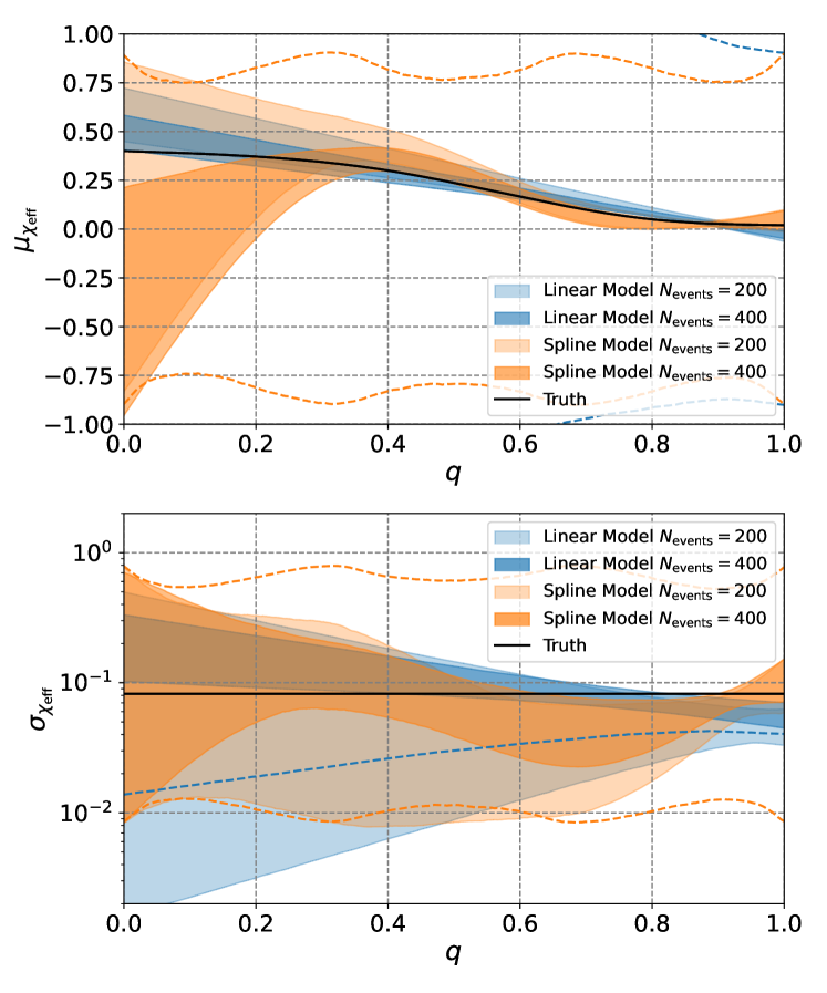
Figure 5: Inferred mean and width of the $\chi_{\rm eff}$ distribution as a function of mass ratio $q$ on two mock catalogs. In blue are the 90% credible intervals when assuming a linear model for the correlation, while in orange are the 90% intervals inferred under the spline model with 4 nodes. The lighter shades represent the inference on a catalog with 200 events, while the darker shade is with 400 events. Dashed lines represent the prior 90% region, and in solid black is the true correlation.

In a catalog of 200 detections, the model evidences indicate no significant preference for a linear model or the spline model. Indeed, the Bayes factor of the spline model over the linear model with 200 events is $\log_{\rm 10}\mathcal{B}_{s|l}(200)=0.00\pm 0.13$. However, when we increase the number of detections to 400, the data begins to indicate a slight preference for the spline model, although nothing yet conclusive; $\log_{\rm 10}\mathcal{B}_{s|l}(400)=0.28\pm 0.14$. We emphasize that this holds for a particular choice of a nonlinear correlation. In truth, the correlation may be more or less linear than the one we simulated, which would make evidence of nonlinearity correspondingly more or less definitive at these numbers of events.

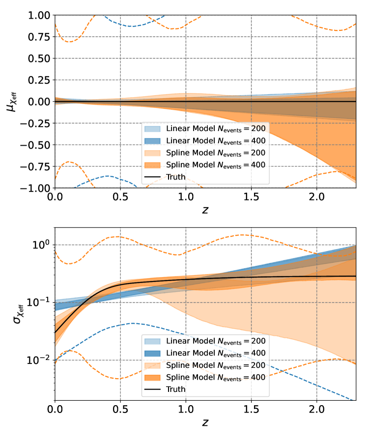
Figure 6: Inferred mean and width of the $\chi_{\rm eff}$ distribution as a function of redshift $z$ on two mock catalogs. In blue are the 90% credible intervals when assuming a linear model for the correlation, while in orange are the 90% intervals inferred under the spline model with 4 nodes. The lighter shades are the inference using a catalog of 200 events, while the darker shade is with 400 events. Dashed lines represent the prior 90% region, and in solid black is the true correlation.

To understand how we may constrain the correlation between the spin population and the redshift in the future, we also simulated a Universe with a nonlinear correlation between the width of the $\chi_{\rm eff}$ distribution and redshift (see Table 2), where the model hyperparameters chosen are consistent with the catalog through the end of the third observing run.

We once again produced mock catalogs with 200 and 400 detections, and we show the results of the inferences in Fig. 6. This time, even a false node placement scheme does a good job at fitting the correlation. Furthermore, model evidences become conclusively in favor of the nonlinear model with a catalog of 400 detections. In particular, for the redshift correlation $\log_{\rm 10}\mathcal{B}_{s|l}(200)=1.06\pm 0.14$ and $\log_{\rm 10}\mathcal{B}_{s|l}(400)=4.09\pm 0.16$. We also checked that a spline model with nodes placed in the correct locations produce consistent results, as expected.

We reiterate that the results of this projection study depend on the assumed true correlation. However, since the correlation we chose is consistent with the data collected thus far, this demonstrates that we can detect nonlinearity in the spin correlation with a catalog of $\sim 400$ detections.

V Conclusions

In this paper we presented a flexible model for understanding the correlation between the spin population in $\chi_{\rm eff}$ and primary mass $m_{1}$, mass ratio $q$ or redshift $z$. On the LVK data published thus far, we obtain results broadly consistent with previous analyses [51, 48, 7, 53, 52]. Furthermore, because of their flexibility, these spline models highlight the regions of parameter space that drive a measured correlation, and the regions of parameter space which are more uncertain.

In particular, we find that the mean of the $\chi_{\rm eff}$ distribution likely increases with mass ratio, the width likely broadens with redshift, and may also broaden for more massive binaries. Importantly, it is also possible that not all of these claims are true at the same time. Perhaps a correlation with one parameter may masquerade as a correlation with another parameter when analyzed under the false hypothesis. Ref. [53] studied this possibility using linear models which simultaneously fit the correlation with $m$, $q$ and $z$, and found that the data is not yet informative enough to answer this question, though it appears possible that all correlations are real. While we do not consider simultaneous models in this work, we do observe the Bayes factors all appear consistent, suggesting the data is not yet informative enough to pick out any mismodeled correlations.

Each of these potential correlations may prove to be important probes of the astrophysical environments which produce BBHs. The observed anticorrelation between the mean of the $\chi_{\rm eff}$ distribution with mass ratio may indicate that the BBHs observed come from binaries which experience mass ratio reversal using an optimistic common envelope (CE) prescription [92], or isolated binaries which either undergo a CE phase with large CE efficiency or stable mass transfer with super-Eddington accretion [93, 43]. It is also possible that hierarchical mergers in a dense environment can produce the observed correlation; we would expect hierarchical mergers involving just one second-generation black hole from a previous merger to have more extreme mass ratios and higher spins [e.g., 47]. However, in an environment with isotropic spin symmetry, the $\chi_{\rm eff}$ distribution must be centered on zero, and so one would expect a broadening of the distribution at small mass ratios, not an increase in the mean. In order to produce the observed correlation, then, the environment must break isotropy symmetry somehow [94], e.g., in an AGN disk [41, 94]. Finally, if the observed BBHs do not originate from one channnel, but a superposition of multiple [e.g., 23, 24], a (linear) correlation may arise from a Simpson’s-type paradox, where multiple populations naturally separated in $\chi_{\rm eff}-q$ space are interpreted as a correlation [26]. Especially in this last scenario, a flexible nonlinear model will help shed light on the origin of the $\chi_{\rm eff}-q$ correlation as we move into O4.

The correlation with redshift probes evidence for other kinds of pathways toward merging stellar mass BBHs. This observation is commonly explained by connecting the spin-up of a BH or its progenitor with the delay time to merger. If the spin-up mechanism of BH progenitors is stronger for closer separations, the remnant BBH system will radiate energy to GWs more rapidly, and hence merge earlier. Because BBHs are born at a higher rate at higher redshifts, this results in a positive correlation between spin magnitude and redshift [95, 37, 96, 97]. One potential mechanism is tidal torques: the spin-up due to tidal torques is amplified if the binary is at a smaller initial separation. If the stellar progenitors retain some angular momentum upon collapse, the BH spins should be correlated with the observed redshift at merger [98, 99, 36]. This is complicated by the expectation that formation in the field produces nearly aligned spins. In this scenario, then there should be a positive correlation between redshift and the mean of the Gaussian; increasing the width requires larger spins with a more isotropic tilt distribution. If there are strong supernova kicks, however, this can even out the spin tilts and give a $\chi_{\rm eff}$ distribution more centered on zero [100, 101, 102, 103].

Finally, a correlation between $\chi_{\rm eff}$ and the primary mass is most naturally understood as a signature of hierarchical mergers. In this paper, we observe a broadening of the $\chi_{\rm eff}$ distribution as the primary mass increases, with varying levels of confidence depending on the model (see appendix §VII.1). This is precisely the expectation of a hierarchical merger picture in an environment endowed with isotropy symmetry [47, 104, 105, 106]. That said, the most recent studies which directly searched for signatures of hierarchical mergers in the LVK catalog strongly disfavor scenarios where all the LVK BBHs are formed hierarchically [107, 108, 109], though they cannot be ruled out as a subpopulation.

To understand how we might probe nonlinear correlations in the future, we also simulated nonlinearly correlated Universes consistent with the data collected thus far. In a Universe with a nonlinear correlation between $\chi_{\rm eff}$ and mass ratio, we found that a linear model may still be appropriate with $\sim 400$ detections, although this is of course heavily dependent on how nonlinear the true correlation is. For a nonlinear correlation in the $z-\chi_{\rm eff}$ plane, we find that a linear model may be significantly disfavored as we approach $\sim 400$ detections. Because the nonlinear correlations we assumed were consistent with LVK data collected thus far, it is possible that linear models for correlation will begin to fail by the end of O4.

However, we also encountered a few drawbacks with spline functions. For one, flexible models are intrinsically high dimensional, and thus sampling from the hyperposterior can become significantly more expensive. Second, spline models are perhaps too good at finding nonlinearities, to the point of confidently finding nonlinear features even when they are not present (see appendix §VII.4). To be confident in a spline-feature, one should recover the feature varying the number of nodes or the locations of the nodes, or even directly estimate the false alarm probability as in Ref. [110].

In this paper, we argue that flexible models for correlation offer a complementary but equally important perspective compared to strongly parameterized models. Foremost, spline models can effectively fit a much wider range of potential correlations. We do not a-priori expect nature to provide us with linear correlations, or even correlations that can be well-approximated by a line [e.g., 44, 45, 46, 47]. The correlations in nature may be strongly nonlinear, or perhaps form as a result of a superposition of subpopulations, and these can only be observed when analyzed with a sufficiently flexible model. Of course, it is possible the correlations will indeed turn out to be linear, however we can only observe such a phenomenon by allowing for the alternative.

VI Acknowledgements

We thank Tom Callister, Matthew Mould, and Colm Talbot for helpful suggestions and relevant expertise. We also thank Christian Adamcewicz for reviewing this work and for providing helpful comments. This material is based upon work supported by NSF’s LIGO Laboratory which is a major facility fully funded by the National Science Foundation. LIGO was constructed by the California Institute of Technology and Massachusetts Institute of Technology with funding from the National Science Foundation and operates under cooperative agreement PHY-0757058. J.H. and S.B. are supported by the NSF Graduate Research Fellowship under Grant No. DGE-1122374. S.B. is also supported by NASA through the NASA Hubble Fellowship grant HST-HF2-51524.001-A awarded by the Space Telescope Science Institute, which is operated by the Association of Universities for Research in Astronomy, Inc., for NASA, under contract NAS5-26555. S.V. is also supported by NSF PHY-2045740. The authors are grateful for computational resources provided by the Caltech LIGO Laboratory and supported by NSF PHY-0757058 and PHY-0823459.

VII Appendix

VII.1 Effective Spin Distribution and Primary Mass

We also search for potential correlation in the population between the $\chi_{\rm eff}$ distribution and the primary mass $m_{1}$. Previous studies have searched for the same correlation (see, e.g., Refs. [51, 53]) using a linear model for the mean and width in Eq. 4, and discovered weak evidence for a trend in the width of the $\chi_{\rm eff}$ distribution.

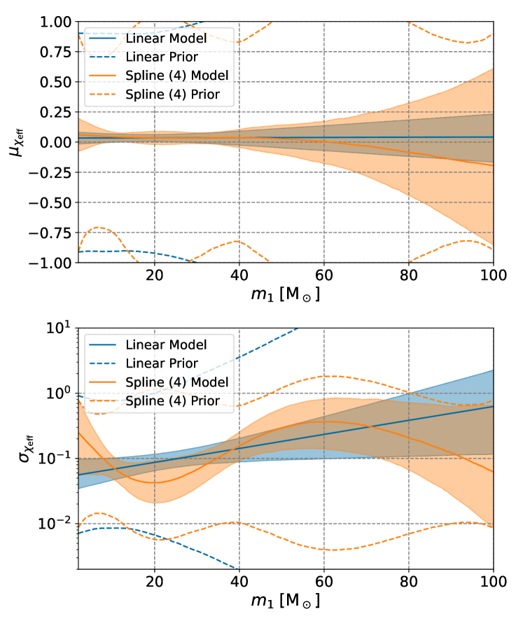
Figure 7: A comparison between the linear model and 4 node spline model for correlation between $\chi_{\rm eff}$ and primary mass, inferred using GWTC-3. Solid lines represent the median, while the shaded region represents the central 90% credible interval, and the dashed lines show the boundary of the prior 90% interval. The upper panel shows the mean of the $\chi_{\rm eff}$ Gaussian as a function of primary mass $m_{1}$, while the lower panel represents the standard deviation of the $\chi_{\rm eff}$ distribution.

Using the same spline approach described above, we place nodes between $m_{\rm 1,min}=2$ and $m_{\rm 1,max}=100$, linearly spaced in $m_{1}^{1/3}$. A uniform node spacing doesn’t easily allow for structure at $\sim 10-30\;M_{\odot}$, which we would like to probe. Instead, linearly spaced in $m_{1}^{1/3}$ clusters nodes towards $m_{1}\sim 10-30\;M_{\odot}$, which we found to be satisfactory.

$$\mu(\theta) =S\left(m_{1}\;|\;(2,\mu_{\chi_{\rm eff}:0}),...,(100,\mu_{\chi_{\rm eff}:N})\right)$$

$$\ln\sigma(\theta) =S\left(m_{1}\;|\;(2,\ln\sigma_{\chi_{\rm eff}:0}),...,(100,\ln\sigma_{\chi_{\rm eff}:N})\right).$$ (8)

We show a comparison between the spline model with 4 nodes and the linear model, in Fig. 7. The linear model and spline models appear broadly consistent; indeed the model evidences do not show any preference for one model over another (see the appendix, Fig. 9. We also show the results for all spline runs in Fig. 10 in the appendix).

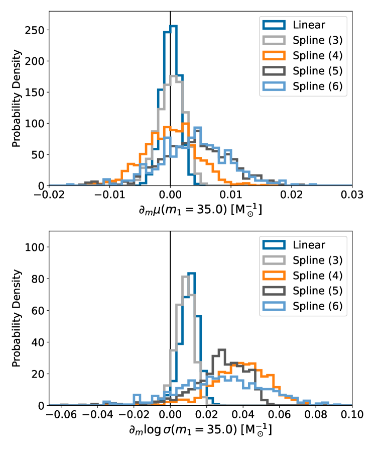
Figure 8: Posteriors on the derivative of the mean and width of the Gaussian as a function of primary mass. Each posterior is broadly consistent, with varying levels of confidence that the slope is greater than zero. The derivative of the mean at $m_{0}=35\;M_{\odot}$ has nearly equal support for being positive of negative, while the derivative of the width is positive at $\sim 85-99.7\%$ confidence for each model.

We also compute the slope of the mean and width at the fiducial value $m_{1}^{*}=35\;M_{\odot}$, and here we find stronger evidence for a positive slope in some spline models than in the linear model. We chose $m_{1}^{*}=35\;M_{\odot}$ to coincide roughly with the location of the Gaussian “peak” in the primary mass distribution [11, 7], and so represents a physically interesting region of parameter space. The linear model finds a broadening at higher primary masses with significance $\sim 93\%$, while the spline models vary in significance, the model with 4 nodes notably exhibits a broadening at $98.7\%$ credence. We show posteriors on the slope at $m_{1}^{*}=35\;M_{\odot}$ in Fig. 8.

VII.2 Inferences on GWTC-3, extra analyses and evidences

We also run each correlation inference with 3-6 nodes for the mean and standard deviation spline functions. For the $\chi_{\rm eff}-q$ correlation, we show the constraints on the mean and standard deviation functions in Fig. 9. We do not observe any strong preference for a including more nodes in the spline correlation functions; there is a generic “Occam’s penalty” for including more nodes beyond what is necessary to appropriately fit the data. We show the evidence of the GWTC-3 data given all our correlation models in Fig. 9; note the evidences are still inconclusive at this stage, though a correlation with mass ratio is somewhat preferred.

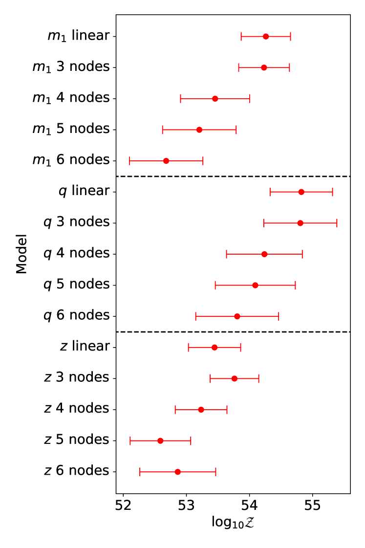
Figure 9: Evidences of the GWTC-3 catalog given each of the $\chi_{\rm eff}$ correlation models. Evidence uncertainties include the average Monte Carlo uncertainty intrinsic to the likelihood estimator, added in quadrature with the nested sampling uncertainty of Dynesty.

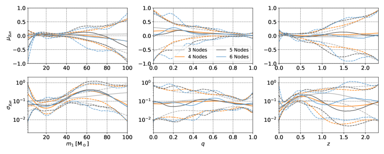
Figure 10: Spline correlations between $\chi_{\rm eff}$ and each parameter we studied, primary mass $m_{1}$ (left column), mass ratio $q$ (center), and redshift $z$ (right). Solid lines represent the median, while the dashed lines represent the boundaries of the central 90% credible interval. The upper panels represents the mean of the $\chi_{\rm eff}$ Gaussian as a function of each parameter, while the lower panels represents the standard deviation of the $\chi_{\rm eff}$ distribution.

	$m_{1}$ (at $m_{1}^{*}=35\;M_{\odot}$)	$q$ (at $q^{*}=0.9$)	$z$ (at $z^{*}=0.2$)
Linear	$p(\partial_{m}\mu>0)=53.9\%$ $p(\partial_{m}\sigma>0)=93.2\%$	$p(\partial_{q}\mu>0)=2.5\%$ $p(\partial_{q}\sigma>0)=41.7\%$	$p(\partial_{z}\mu>0)=16.2\%$ $p(\partial_{z}\sigma>0)=92.7\%$
Spline (3)	$p(\partial_{m}\mu>0)=55.0\%$ $p(\partial_{m}\sigma>0)=89.5\%$	$p(\partial_{q}\mu>0)=13.4\%$ $p(\partial_{q}\sigma>0)=33.0\%$	$p(\partial_{z}\mu>0)=14.2\%$ $p(\partial_{z}\sigma>0)=95.6\%$
Spline (4)	$p(\partial_{m}\mu>0)=60.5\%$ $p(\partial_{m}\sigma>0)=98.7\%$	$p(\partial_{q}\mu>0)=18.7\%$ $p(\partial_{q}\sigma>0)=44.5\%$	$p(\partial_{z}\mu>0)=19.6\%$ $p(\partial_{z}\sigma>0)=98.0\%$
Spline (5)	$p(\partial_{m}\mu>0)=78.3\%$ $p(\partial_{m}\sigma>0)=95.7\%$	$p(\partial_{q}\mu>0)=21.7\%$ $p(\partial_{q}\sigma>0)=58.1\%$	$p(\partial_{z}\mu>0)=17.0\%$ $p(\partial_{z}\sigma>0)=88.8\%$
Spline (6)	$p(\partial_{m}\mu>0)=77.8\%$ $p(\partial_{m}\sigma>0)=93.6\%$	$p(\partial_{q}\mu>0)=30.0\%$ $p(\partial_{q}\sigma>0)=65.5\%$	$p(\partial_{z}\mu>0)=5.9\%$ $p(\partial_{z}\sigma>0)=98.6\%$

Table 3: Credibility of a positive slope in the evolution of the mean (denoted $\delta\mu>0$) at the fiducial value, and of a positive slope in the evolution of the width (denoted $\delta\sigma>0$). The column on the left is the model assumed, where “Spline ($N$)” refers to the spline model using $N$ nodes. In each cell, the top line represents the credibility of a positive slope in the mean, and the bottom line represents the same quantity for the width.

VII.3 Nonlinear Correlation in $\chi_{\rm eff}-z$

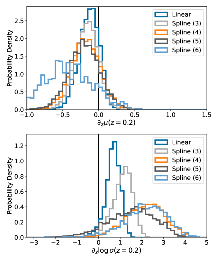
Figure 11: Posteriors on the derivative of the mean and width of the Gaussian with respect to redshift at $z^{*}=0.2$, inferred on GWTC-3 data. Each posterior is consistent, with varying levels of confidence that the slope is greater than zero.

To study the potential risk of inferring a nonlinear correlation a GWTC-3-like catalog from a linearly correlated Universe, we used 12 sets of 69 detections drawn from a uncorrelated Universe observed with Hanford and Livingston in O4-like PSDs [86], in a similar process to the method presented in §IV. These synthetic events were injected from a linearly correlated Universe (namely, uncorrelated with slope zero), with a mean $\mu_{\chi_{\rm eff}}=0.06$ and width $\sigma_{\chi_{\rm eff}}=0.11$, and the same thresholds, waveforms, and PE techniques described in §IV. Then, we infer the $\chi_{\rm eff}$ correlation with respect to the redshift $z$ for each synthetic catalog, using the method we introduced in §III. We compute the instantaneous slope at the first three nodes for each hyperposterior sample, and can then estimate the JS divergence between the posteriors of the slopes at neighboring nodes.

We also show the slope posteriors at a fiducial value $z^{*}=0.2$ in Fig. 11. We avoid choosing $z^{*}=0$, as the data is uninformative in the limit of $z\to 0$ for the same reason it is uninformative for $q\to 0$. While some of the 69 BBH events are closer than others, none of them are consistent with being at $z\to 0$, and indeed it is baked into the population model where the probability density at a given redshift is proportional to the differential comoving volume $p(z)\propto\frac{dV_{c}}{dz}$ to have zero support at $z\to 0$ [111, 65]. In other words, a flexible $z-\chi_{\rm eff}$ correlation model, in particular spline models with appropriate node density and placement, will increase in uncertainty as $z\to 0$. Indeed, we observe this to some degree in each spline model in Fig. 10, but it is especially clear in the spline model with 5 nodes.

We also should note the significance of broadening with redshift using the linear model is only 92.7%, while Ref. [53] inferred a broadening at 98.6% credibility. We checked various differences between our analyses, and discovered that this difference arises from how selection effects are estimated. In particular, Ref. [53] assumes a semi-analytic threshold on the network SNR $\rho_{\rm net}>9$ for O1 and O2 events, while we use a threshold of $\rho_{\rm net}>10$, following Ref. [7].

VII.4 Node Placement and Bias in Mock Catalogs

In §IV we study a Universe with a nonlinear correlation in the $\chi_{\rm eff}-q$ plane. We find that, when we fix the x-axis positions of the nodes to be different than the true node positions, we may recover some bias in the inference.

Specifically, the results in Fig. 5 highlight one of the drawbacks for using spline models. Fitting a spline model to a smooth function often results in extraneous structure, bumps that the spline function cannot remove entirely due to its functional form [110]. In the case of the mock catalog we simulated, the correlation is created using a spline node placement (Table 2) different from the spline node placement scheme we recover with. Because of this, the spline cannot simultaneously fit the correlation in the region of near equal mass ratio while also effectively fitting the region of more extreme mass ratios, and so it must compromise with a suboptimal fit across the parameter space. Hence the spline model “wiggles” when it ideally should be smooth.

Because we are not yet in the limit of infinitely many nodes (we use 4 nodes in this inference), the spline functions are not perfectly flexible. More nodes are inherently more flexible, and so would presumably do a better job at fitting the correlation. Similarly, using a correct node placement scheme should also improve the fit. Indeed, we find that when we analyze the mock catalog using the same node positions as the true correlation (Table 2), the inferred correlation is closer to the truth. This highlights the importance of either running with multiple node counts and placement schemes, or marginalizing over the node x-axis positions as well.

References

- Abbott et al. [2021] R. Abbott et al. (LIGO Scientific, VIRGO, KAGRA), GWTC-3: Compact Binary Coalescences Observed by LIGO and Virgo During the Second Part of the Third Observing Run (2021), arXiv:2111.03606 [gr-qc] .
- Aasi et al. [2015] J. Aasi et al. (LIGO Scientific), Advanced LIGO, Class. Quant. Grav. 32, 074001 (2015), arXiv:1411.4547 [gr-qc] .
- Acernese et al. [2015] F. Acernese et al. (VIRGO), Advanced Virgo: a second-generation interferometric gravitational wave detector, Class. Quant. Grav. 32, 024001 (2015), arXiv:1408.3978 [gr-qc] .
- Aso et al. [2013] Y. Aso, Y. Michimura, K. Somiya, M. Ando, O. Miyakawa, T. Sekiguchi, D. Tatsumi, and H. Yamamoto (KAGRA), Interferometer design of the KAGRA gravitational wave detector, Phys. Rev. D 88, 043007 (2013), arXiv:1306.6747 [gr-qc] .
- Somiya [2012] K. Somiya (KAGRA), Detector configuration of KAGRA: The Japanese cryogenic gravitational-wave detector, Class. Quant. Grav. 29, 124007 (2012), arXiv:1111.7185 [gr-qc] .
- Akutsu et al. [2021] T. Akutsu et al. (KAGRA), Overview of KAGRA: Detector design and construction history, PTEP 2021, 05A101 (2021), arXiv:2005.05574 [physics.ins-det] .
- Abbott et al. [2023] R. Abbott et al. (KAGRA, VIRGO, LIGO Scientific), Population of Merging Compact Binaries Inferred Using Gravitational Waves through GWTC-3, Phys. Rev. X 13, 011048 (2023), arXiv:2111.03634 [astro-ph.HE] .
- Tiwari and Fairhurst [2021] V. Tiwari and S. Fairhurst, The Emergence of Structure in the Binary Black Hole Mass Distribution, Astrophys. J. Lett. 913, L19 (2021), arXiv:2011.04502 [astro-ph.HE] .
- Edelman et al. [2022] B. Edelman, Z. Doctor, J. Godfrey, and B. Farr, Ain’t No Mountain High Enough: Semiparametric Modeling of LIGO–Virgo’s Binary Black Hole Mass Distribution, Astrophys. J. 924, 101 (2022), arXiv:2109.06137 [astro-ph.HE] .
- Fishbach and Holz [2017] M. Fishbach and D. E. Holz, Where Are LIGO’s Big Black Holes?, Astrophys. J. Lett. 851, L25 (2017), arXiv:1709.08584 [astro-ph.HE] .
- Talbot and Thrane [2018] C. Talbot and E. Thrane, Measuring the binary black hole mass spectrum with an astrophysically motivated parameterization, Astrophys. J. 856, 173 (2018), arXiv:1801.02699 [astro-ph.HE] .
- Fishbach and Holz [2020] M. Fishbach and D. E. Holz, Picky Partners: The Pairing of Component Masses in Binary Black Hole Mergers, Astrophys. J. Lett. 891, L27 (2020), arXiv:1905.12669 [astro-ph.HE] .
- Farah et al. [2023a] A. M. Farah, M. Fishbach, and D. E. Holz, Two of a Kind: Comparing big and small black holes in binaries with gravitational waves (2023a), arXiv:2308.05102 [astro-ph.HE] .
- Wysocki et al. [2019] D. Wysocki, J. Lange, and R. O’Shaughnessy, Reconstructing phenomenological distributions of compact binaries via gravitational wave observations, Phys. Rev. D 100, 043012 (2019).
- Biscoveanu et al. [2021] S. Biscoveanu, M. Isi, S. Vitale, and V. Varma, New Spin on LIGO-Virgo Binary Black Holes, Phys. Rev. Lett. 126, 171103 (2021), arXiv:2007.09156 [astro-ph.HE] .
- Callister et al. [2022] T. A. Callister, S. J. Miller, K. Chatziioannou, and W. M. Farr, No Evidence that the Majority of Black Holes in Binaries Have Zero Spin, Astrophys. J. Lett. 937, L13 (2022), arXiv:2205.08574 [astro-ph.HE] .
- Tong et al. [2022] H. Tong, S. Galaudage, and E. Thrane, Population properties of spinning black holes using the gravitational-wave transient catalog 3, Phys. Rev. D 106, 103019 (2022), arXiv:2209.02206 [astro-ph.HE] .
- Mould et al. [2022] M. Mould, D. Gerosa, F. S. Broekgaarden, and N. Steinle, Which black hole formed first? Mass-ratio reversal in massive binary stars from gravitational-wave data, Mon. Not. Roy. Astron. Soc. 517, 2738 (2022), arXiv:2205.12329 [astro-ph.HE] .
- Galaudage et al. [2021] S. Galaudage et al., Building Better Spin Models for Merging Binary Black Holes: Evidence for Nonspinning and Rapidly Spinning Nearly Aligned Subpopulations, Astrophys. J. Lett. 921, L15 (2021), [Erratum: Astrophys.J.Lett. 936, L18 (2022), Erratum: Astrophys.J. 936, L18 (2022)], arXiv:2109.02424 [gr-qc] .
- Roulet et al. [2021] J. Roulet, H. S. Chia, S. Olsen, L. Dai, T. Venumadhav, B. Zackay, and M. Zaldarriaga, Distribution of effective spins and masses of binary black holes from the LIGO and Virgo O1–O3a observing runs, Phys. Rev. D 104, 083010 (2021), arXiv:2105.10580 [astro-ph.HE] .
- Vitale et al. [2022] S. Vitale, S. Biscoveanu, and C. Talbot, Spin it as you like: The (lack of a) measurement of the spin tilt distribution with LIGO-Virgo-KAGRA binary black holes, Astron. Astrophys. 668, L2 (2022), arXiv:2209.06978 [astro-ph.HE] .
- Fishbach et al. [2021] M. Fishbach, Z. Doctor, T. Callister, B. Edelman, J. Ye, R. Essick, W. M. Farr, B. Farr, and D. E. Holz, When Are LIGO/Virgo’s Big Black Hole Mergers?, Astrophys. J. 912, 98 (2021), arXiv:2101.07699 [astro-ph.HE] .
- Zevin et al. [2021] M. Zevin, S. S. Bavera, C. P. L. Berry, V. Kalogera, T. Fragos, P. Marchant, C. L. Rodriguez, F. Antonini, D. E. Holz, and C. Pankow, One Channel to Rule Them All? Constraining the Origins of Binary Black Holes Using Multiple Formation Pathways, Astrophys. J. 910, 152 (2021), arXiv:2011.10057 [astro-ph.HE] .
- Cheng et al. [2023] A. Q. Cheng, M. Zevin, and S. Vitale, What You Don’t Know Can Hurt You: Use and Abuse of Astrophysical Models in Gravitational-wave Population Analyses, Astrophys. J. 955, 127 (2023), arXiv:2307.03129 [astro-ph.HE] .
- Wong et al. [2021] K. W. K. Wong, K. Breivik, K. Kremer, and T. Callister, Joint constraints on the field-cluster mixing fraction, common envelope efficiency, and globular cluster radii from a population of binary hole mergers via deep learning, Phys. Rev. D 103, 083021 (2021), arXiv:2011.03564 [astro-ph.HE] .
- Baibhav et al. [2023] V. Baibhav, Z. Doctor, and V. Kalogera, Dropping Anchor: Understanding the Populations of Binary Black Holes with Random and Aligned-spin Orientations, Astrophys. J. 946, 50 (2023), arXiv:2212.12113 [astro-ph.HE] .
- Godfrey et al. [2023] J. Godfrey, B. Edelman, and B. Farr, Cosmic Cousins: Identification of a Subpopulation of Binary Black Holes Consistent with Isolated Binary Evolution (2023), arXiv:2304.01288 [astro-ph.HE] .
- Wang et al. [2022] Y.-Z. Wang, Y.-J. Li, J. S. Vink, Y.-Z. Fan, S.-P. Tang, Y. Qin, and D.-M. Wei, Potential Subpopulations and Assembling Tendency of the Merging Black Holes, Astrophys. J. Lett. 941, L39 (2022), arXiv:2208.11871 [astro-ph.HE] .
- Edelman et al. [2023] B. Edelman, B. Farr, and Z. Doctor, Cover Your Basis: Comprehensive Data-driven Characterization of the Binary Black Hole Population, Astrophys. J. 946, 16 (2023), arXiv:2210.12834 [astro-ph.HE] .
- Golomb and Talbot [2023] J. Golomb and C. Talbot, Searching for structure in the binary black hole spin distribution, Phys. Rev. D 108, 103009 (2023), arXiv:2210.12287 [astro-ph.HE] .
- Rinaldi and Del Pozzo [2021] S. Rinaldi and W. Del Pozzo, (H)DPGMM: a hierarchy of Dirichlet process Gaussian mixture models for the inference of the black hole mass function, Mon. Not. Roy. Astron. Soc. 509, 5454 (2021), arXiv:2109.05960 [astro-ph.IM] .
- Tiwari [2021] V. Tiwari, VAMANA: modeling binary black hole population with minimal assumptions, Class. Quant. Grav. 38, 155007 (2021), arXiv:2006.15047 [astro-ph.HE] .
- Tiwari [2022] V. Tiwari, Exploring Features in the Binary Black Hole Population, Astrophys. J. 928, 155 (2022), arXiv:2111.13991 [astro-ph.HE] .
- Callister and Farr [2023] T. A. Callister and W. M. Farr, A Parameter-Free Tour of the Binary Black Hole Population (2023), arXiv:2302.07289 [astro-ph.HE] .
- Romero-Shaw et al. [2022] I. M. Romero-Shaw, E. Thrane, and P. D. Lasky, When models fail: An introduction to posterior predictive checks and model misspecification in gravitational-wave astronomy, Publ. Astron. Soc. Austral. 39, e025 (2022), arXiv:2202.05479 [astro-ph.IM] .
- Bavera et al. [2022] S. S. Bavera, M. Fishbach, M. Zevin, E. Zapartas, and T. Fragos, The eff z correlation of field binary black hole mergers and how 3G gravitational-wave detectors can constrain it, Astron. Astrophys. 665, A59 (2022), arXiv:2204.02619 [astro-ph.HE] .
- Bavera et al. [2020] S. S. Bavera, T. Fragos, Y. Qin, E. Zapartas, C. J. Neijssel, I. Mandel, A. Batta, S. M. Gaebel, C. Kimball, and S. Stevenson, The origin of spin in binary black holes: Predicting the distributions of the main observables of Advanced LIGO, Astron. Astrophys. 635, A97 (2020), arXiv:1906.12257 [astro-ph.HE] .
- McKernan et al. [2012] B. McKernan, K. E. S. Ford, W. Lyra, and H. B. Perets, Intermediate mass black holes in AGN disks: I. Production & Growth, Mon. Not. Roy. Astron. Soc. 425, 460 (2012), arXiv:1206.2309 [astro-ph.GA] .
- Stone et al. [2017] N. C. Stone, B. D. Metzger, and Z. Haiman, Assisted inspirals of stellar mass black holes embedded in AGN discs: solving the ‘final au problem’, Mon. Not. Roy. Astron. Soc. 464, 946 (2017), arXiv:1602.04226 [astro-ph.GA] .
- McKernan et al. [2020] B. McKernan, K. E. S. Ford, R. O’Shaughnessy, and D. Wysocki, Monte Carlo simulations of black hole mergers in AGN discs: Low mergers and predictions for LIGO, Mon. Not. Roy. Astron. Soc. 494, 1203 (2020), arXiv:1907.04356 [astro-ph.HE] .
- McKernan et al. [2022] B. McKernan, K. E. S. Ford, T. Callister, W. M. Farr, R. O’Shaughnessy, R. Smith, E. Thrane, and A. Vajpeyi, LIGO–Virgo correlations between mass ratio and effective inspiral spin: testing the active galactic nuclei channel, Mon. Not. Roy. Astron. Soc. 514, 3886 (2022), arXiv:2107.07551 [astro-ph.HE] .
- Tagawa et al. [2020] H. Tagawa, Z. Haiman, and B. Kocsis, Formation and Evolution of Compact Object Binaries in AGN Disks, Astrophys. J. 898, 25 (2020), arXiv:1912.08218 [astro-ph.GA] .
- Zevin and Bavera [2022] M. Zevin and S. S. Bavera, Suspicious Siblings: The Distribution of Mass and Spin across Component Black Holes in Isolated Binary Evolution, Astrophys. J. 933, 86 (2022), arXiv:2203.02515 [astro-ph.HE] .
- Belczynski et al. [2020] K. Belczynski et al., Evolutionary roads leading to low effective spins, high black hole masses, and O1/O2 rates for LIGO/Virgo binary black holes, Astron. Astrophys. 636, A104 (2020), arXiv:1706.07053 [astro-ph.HE] .
- Portegies Zwart and McMillan [2002] S. F. Portegies Zwart and S. L. W. McMillan, The Runaway growth of intermediate-mass black holes in dense star clusters, Astrophys. J. 576, 899 (2002), arXiv:astro-ph/0201055 .
- Rodriguez et al. [2015] C. L. Rodriguez, M. Morscher, B. Pattabiraman, S. Chatterjee, C.-J. Haster, and F. A. Rasio, Binary Black Hole Mergers from Globular Clusters: Implications for Advanced LIGO, Phys. Rev. Lett. 115, 051101 (2015), [Erratum: Phys.Rev.Lett. 116, 029901 (2016)], arXiv:1505.00792 [astro-ph.HE] .
- Gerosa and Fishbach [2021] D. Gerosa and M. Fishbach, Hierarchical mergers of stellar-mass black holes and their gravitational-wave signatures, Nature Astron. 5, 8 (2021), arXiv:2105.03439 [astro-ph.HE] .
- Callister et al. [2021a] T. A. Callister, C.-J. Haster, K. K. Y. Ng, S. Vitale, and W. M. Farr, Who Ordered That? Unequal-mass Binary Black Hole Mergers Have Larger Effective Spins, Astrophys. J. Lett. 922, L5 (2021a), arXiv:2106.00521 [astro-ph.HE] .
- Adamcewicz and Thrane [2022] C. Adamcewicz and E. Thrane, Do unequal-mass binary black hole systems have larger eff? Probing correlations with copulas in gravitational-wave astronomy, Mon. Not. Roy. Astron. Soc. 517, 3928 (2022), arXiv:2208.03405 [astro-ph.HE] .
- Adamcewicz et al. [2023] C. Adamcewicz, P. D. Lasky, and E. Thrane, Evidence for a Correlation between Binary Black Hole Mass Ratio and Black Hole Spins, Astrophys. J. 958, 13 (2023), arXiv:2307.15278 [astro-ph.HE] .
- Safarzadeh et al. [2020] M. Safarzadeh, W. M. Farr, and E. Ramirez-Ruiz, A trend in the effective spin distribution of LIGO binary black holes with mass, Astrophys. J. 894, 129 (2020), arXiv:2001.06490 [gr-qc] .
- Franciolini and Pani [2022] G. Franciolini and P. Pani, Searching for mass-spin correlations in the population of gravitational-wave events: The GWTC-3 case study, Phys. Rev. D 105, 123024 (2022), arXiv:2201.13098 [astro-ph.HE] .
- Biscoveanu et al. [2022] S. Biscoveanu, T. A. Callister, C.-J. Haster, K. K. Y. Ng, S. Vitale, and W. M. Farr, The Binary Black Hole Spin Distribution Likely Broadens with Redshift, Astrophys. J. Lett. 932, L19 (2022), arXiv:2204.01578 [astro-ph.HE] .
- Rinaldi et al. [2023] S. Rinaldi, W. Del Pozzo, M. Mapelli, A. L. Medina, and T. Dent, Evidence for the evolution of black hole mass function with redshift (2023), arXiv:2310.03074 [astro-ph.HE] .
- van Son et al. [2022] L. A. C. van Son, S. E. de Mink, T. Callister, S. Justham, M. Renzo, T. Wagg, F. S. Broekgaarden, F. Kummer, R. Pakmor, and I. Mandel, The Redshift Evolution of the Binary Black Hole Merger Rate: A Weighty Matter, Astrophys. J. 931, 17 (2022), arXiv:2110.01634 [astro-ph.HE] .
- Loredo [2004] T. J. Loredo, Accounting for source uncertainties in analyses of astronomical survey data, in Bayesian Inference and Maximum Entropy Methods in Science and Engineering ed R. Fischer, R. Preuss and U. V. Toussaint, AIP Conference Series, Vol. 735 (AIP, Melville, NY, 2004) p. 195.
- Farr et al. [2015] W. M. Farr, J. R. Gair, I. Mandel, and C. Cutler, Counting And Confusion: Bayesian Rate Estimation With Multiple Populations, Phys. Rev. D 91, 023005 (2015), arXiv:1302.5341 [astro-ph.IM] .
- Foreman-Mackey et al. [2014] D. Foreman-Mackey, D. W. Hogg, and T. D. Morton, Exoplanet population inference and the abundance of earth analogs from noise, incomplete catalogs, The Astrophysical Journal 795, 64 (2014).
- Mandel et al. [2019] I. Mandel, W. M. Farr, and J. R. Gair, Extracting distribution parameters from multiple uncertain observations with selection biases, MNRAS 486, 1086 (2019), http://oup.prod.sis.lan/mnras/article-pdf/486/1/1086/28390969/stz896.pdf .
- Vitale [2020] S. Vitale, One, No One, and One Hundred Thousand – Inferring the properties of a population in presence of selection effects (2020), arXiv:2007.05579 [astro-ph.IM] .
- Essick and Fishbach [2023] R. Essick and M. Fishbach, DAGnabbit! Ensuring Consistency between Noise and Detection in Hierarchical Bayesian Inference (2023), arXiv:2310.02017 [gr-qc] .
- Farr [2019] W. M. Farr, Accuracy requirements for empirically measured selection functions, Research Notes of the AAS 3, 66 (2019).
- Essick and Farr [2022] R. Essick and W. Farr, Precision Requirements for Monte Carlo Sums within Hierarchical Bayesian Inference (2022), arXiv:2204.00461 [astro-ph.IM] .
- Talbot and Golomb [2023] C. Talbot and J. Golomb, Growing pains: understanding the impact of likelihood uncertainty on hierarchical Bayesian inference for gravitational-wave astronomy, Mon. Not. Roy. Astron. Soc. 526, 3495 (2023), arXiv:2304.06138 [astro-ph.IM] .
- Fishbach et al. [2018] M. Fishbach, D. E. Holz, and W. M. Farr, Does the Black Hole Merger Rate Evolve with Redshift?, Astrophys. J. Lett. 863, L41 (2018), arXiv:1805.10270 [astro-ph.HE] .
- Damour [2001] T. Damour, Coalescence of two spinning black holes: An effective one-body approach, Phys. Rev. D 64, 124013 (2001).
- Racine [2008] E. Racine, Analysis of spin precession in binary black hole systems including quadrupole-monopole interaction, Phys. Rev. D 78, 044021 (2008), arXiv:0803.1820 [gr-qc] .
- Ajith et al. [2011] P. Ajith et al., Inspiral-merger-ringdown waveforms for black-hole binaries with non-precessing spins, Phys. Rev. Lett. 106, 241101 (2011), arXiv:0909.2867 [gr-qc] .
- Vitale et al. [2017] S. Vitale, R. Lynch, V. Raymond, R. Sturani, J. Veitch, and P. Graff, Parameter estimation for heavy binary-black holes with networks of second-generation gravitational-wave detectors, Phys. Rev. D 95, 064053 (2017), arXiv:1611.01122 [gr-qc] .
- Pürrer et al. [2016] M. Pürrer, M. Hannam, and F. Ohme, Can we measure individual black-hole spins from gravitational-wave observations?, Phys. Rev. D 93, 084042 (2016), arXiv:1512.04955 [gr-qc] .
- Miller et al. [2020] S. Miller, T. A. Callister, and W. Farr, The Low Effective Spin of Binary Black Holes and Implications for Individual Gravitational-Wave Events, Astrophys. J. 895, 128 (2020), arXiv:2001.06051 [astro-ph.HE] .
- Roulet and Zaldarriaga [2019] J. Roulet and M. Zaldarriaga, Constraints on binary black hole populations from LIGO–Virgo detections, Mon. Not. Roy. Astron. Soc. 484, 4216 (2019), arXiv:1806.10610 [astro-ph.HE] .
- de Boor [1976] C. de Boor, On cubic spline functions that vanish at all knots, Advances in Mathematics 20, 1 (1976).
- LIGO Scientific Collaboration et al. [2020] LIGO Scientific Collaboration, Virgo Collaboration, and KAGRA Collaboration, Parameter estimation sample release for GWTC-1, Tech. Rep. P1800370 (LVK, 2020).
- LIGO Scientific Collaboration et al. [2021] LIGO Scientific Collaboration, Virgo Collaboration, and KAGRA Collaboration, GWTC-2 Data Release: Parameter Estimation Samples and Skymaps, Tech. Rep. P2000223 (LVK, 2021).
- LIGO Scientific Collaboration and Virgo Collaboration [2022] LIGO Scientific Collaboration and Virgo Collaboration, GWTC-2.1: Deep Extended Catalog of Compact Binary Coalescences Observed by LIGO and Virgo During the First Half of the Third Observing Run - Parameter Estimation Data Release, 10.5281/zenodo.6513631 (2022).
- LIGO Scientific Collaboration et al. [2023a] LIGO Scientific Collaboration, Virgo Collaboration, and KAGRA Collaboration, GWTC-3: Compact Binary Coalescences Observed by LIGO and Virgo During the Second Part of the Third Observing Run — Parameter estimation data release, 10.5281/zenodo.8177023 (2023a).
- LIGO Scientific Collaboration et al. [2023b] LIGO Scientific Collaboration, Virgo Collaboration, and KAGRA Collaboration, GWTC-3: Compact Binary Coalescences Observed by LIGO and Virgo During the Second Part of the Third Observing Run — O1+O2+O3 Search Sensitivity Estimates, 10.5281/zenodo.7890398 (2023b).
- Talbot et al. [2019] C. Talbot, R. Smith, E. Thrane, and G. B. Poole, Parallelized inference for gravitational-wave astronomy, Phys. Rev. D 100, 043030 (2019).
- Speagle [2020] J. S. Speagle, dynesty: a dynamic nested sampling package for estimating Bayesian posteriors and evidences, MNRAS 493, 3132 (2020), https://academic.oup.com/mnras/article-pdf/493/3/3132/32890730/staa278.pdf .
- Ashton et al. [2019] G. Ashton et al., BILBY: A user-friendly Bayesian inference library for gravitational-wave astronomy, Astrophys. J. Suppl. 241, 27 (2019), arXiv:1811.02042 [astro-ph.IM] .
- Note [1] Though is an unphysical region of parameter space with no observations, the node at should be thought of as simply a parameter necessary to ensure the model is defined over the entire space (any distribution must be defined over the full parameter space), and not an a priori statement that BBHs exist here; indeed the smoothed powerlaw is always zero at .
- Note [2] This is somewhat at odds with the maximum redshift considered in the sensitivity injections of [78], with . We verified our results are unchanged after considering this adjustment.
- Kullback and Leibler [1951] S. Kullback and R. A. Leibler, On information and sufficiency, Ann. Math. Statist. 22, 79 (1951).
- Lin [1991] J. Lin, Divergence measures based on the Shannon entropy, IEEE Trans. Info. Theor. 37, 145 (1991).
- Abbott et al. [2020] B. Abbott et al. (KAGRA, LIGO Scientific, Virgo, VIRGO), Noise curves used for simulations in the update of the observing scenarios paper (2020).
- Pratten et al. [2021] G. Pratten et al., Computationally efficient models for the dominant and subdominant harmonic modes of precessing binary black holes, Phys. Rev. D 103, 104056 (2021), arXiv:2004.06503 [gr-qc] .
- Cornish [2010] N. J. Cornish, Fast Fisher Matrices and Lazy Likelihoods (2010), arXiv:1007.4820 [gr-qc] .
- Cornish [2021] N. J. Cornish, Heterodyned likelihood for rapid gravitational wave parameter inference, Phys. Rev. D 104, 104054 (2021), arXiv:2109.02728 [gr-qc] .
- Zackay et al. [2018] B. Zackay, L. Dai, and T. Venumadhav, Relative Binning and Fast Likelihood Evaluation for Gravitational Wave Parameter Estimation (2018), arXiv:1806.08792 [astro-ph.IM] .
- Essick [2023] R. Essick, Semianalytic sensitivity estimates for catalogs of gravitational-wave transients, Phys. Rev. D 108, 043011 (2023), arXiv:2307.02765 [gr-qc] .
- Broekgaarden et al. [2022] F. S. Broekgaarden, S. Stevenson, and E. Thrane, Signatures of Mass Ratio Reversal in Gravitational Waves from Merging Binary Black Holes, Astrophys. J. 938, 45 (2022), arXiv:2205.01693 [astro-ph.HE] .
- Bavera et al. [2021a] S. S. Bavera et al., The impact of mass-transfer physics on the observable properties of field binary black hole populations, Astron. Astrophys. 647, A153 (2021a), arXiv:2010.16333 [astro-ph.HE] .
- Santini et al. [2023] A. Santini, D. Gerosa, R. Cotesta, and E. Berti, Black-hole mergers in disklike environments could explain the observed q-eff correlation, Phys. Rev. D 108, 083033 (2023), arXiv:2308.12998 [astro-ph.HE] .
- Zaldarriaga et al. [2018] M. Zaldarriaga, D. Kushnir, and J. A. Kollmeier, The expected spins of gravitational wave sources with isolated field binary progenitors, Mon. Not. Roy. Astron. Soc. 473, 4174 (2018), arXiv:1702.00885 [astro-ph.HE] .
- Bavera et al. [2021b] S. S. Bavera, M. Zevin, and T. Fragos, Approximations to the spin of close Black-hole-Wolf-Rayet binaries (2021b), arXiv:2105.09077 [astro-ph.HE] .
- Fuller and Lu [2022] J. Fuller and W. Lu, The spins of compact objects born from helium stars in binary systems, Mon. Not. Roy. Astron. Soc. 511, 3951 (2022), arXiv:2201.08407 [astro-ph.HE] .
- Qin et al. [2018] Y. Qin, T. Fragos, G. Meynet, J. Andrews, M. Sørensen, and H. F. Song, The spin of the second-born black hole in coalescing binary black holes, Astron. Astrophys. 616, A28 (2018), arXiv:1802.05738 [astro-ph.SR] .
- Fuller and Ma [2019] J. Fuller and L. Ma, Most Black Holes are Born Very Slowly Rotating, Astrophys. J. Lett. 881, L1 (2019), arXiv:1907.03714 [astro-ph.SR] .
- Rodriguez et al. [2016] C. L. Rodriguez, M. Zevin, C. Pankow, V. Kalogera, and F. A. Rasio, Illuminating Black Hole Binary Formation Channels with Spins in Advanced LIGO, Astrophys. J. Lett. 832, L2 (2016), arXiv:1609.05916 [astro-ph.HE] .
- Gerosa et al. [2018] D. Gerosa, E. Berti, R. O’Shaughnessy, K. Belczynski, M. Kesden, D. Wysocki, and W. Gladysz, Spin orientations of merging black holes formed from the evolution of stellar binaries, Phys. Rev. D 98, 084036 (2018), arXiv:1808.02491 [astro-ph.HE] .
- Callister et al. [2021b] T. A. Callister, W. M. Farr, and M. Renzo, State of the Field: Binary Black Hole Natal Kicks and Prospects for Isolated Field Formation after GWTC-2, Astrophys. J. 920, 157 (2021b), arXiv:2011.09570 [astro-ph.HE] .
- Stevenson [2022] S. Stevenson, Biases in Estimates of Black Hole Kicks from the Spin Distribution of Binary Black Holes, Astrophys. J. Lett. 926, L32 (2022), arXiv:2202.03584 [astro-ph.HE] .
- Gerosa and Berti [2017] D. Gerosa and E. Berti, Are merging black holes born from stellar collapse or previous mergers?, Phys. Rev. D 95, 124046 (2017), arXiv:1703.06223 [gr-qc] .
- Fishbach et al. [2017] M. Fishbach, D. E. Holz, and B. Farr, Are LIGO’s Black Holes Made From Smaller Black Holes?, Astrophys. J. Lett. 840, L24 (2017), arXiv:1703.06869 [astro-ph.HE] .
- Tagawa et al. [2021] H. Tagawa, Z. Haiman, I. Bartos, B. Kocsis, and K. Omukai, Signatures of hierarchical mergers in black hole spin and mass distribution, Mon. Not. Roy. Astron. Soc. 507, 3362 (2021), arXiv:2104.09510 [astro-ph.HE] .
- Fishbach et al. [2022] M. Fishbach, C. Kimball, and V. Kalogera, Limits on Hierarchical Black Hole Mergers from the Most Negative eff Systems, Astrophys. J. Lett. 935, L26 (2022), arXiv:2207.02924 [astro-ph.HE] .
- Doctor et al. [2019] Z. Doctor, D. Wysocki, R. O’Shaughnessy, D. E. Holz, and B. Farr, Black Hole Coagulation: Modeling Hierarchical Mergers in Black Hole Populations (2019), arXiv:1911.04424 [astro-ph.HE] .
- Kimball et al. [2020] C. Kimball, C. Talbot, C. P. L. Berry, M. Carney, M. Zevin, E. Thrane, and V. Kalogera, Black Hole Genealogy: Identifying Hierarchical Mergers with Gravitational Waves, Astrophys. J. 900, 177 (2020), arXiv:2005.00023 [astro-ph.HE] .
- Farah et al. [2023b] A. M. Farah, B. Edelman, M. Zevin, M. Fishbach, J. M. Ezquiaga, B. Farr, and D. E. Holz, Things That Might Go Bump in the Night: Assessing Structure in the Binary Black Hole Mass Spectrum, Astrophys. J. 955, 107 (2023b), arXiv:2301.00834 [astro-ph.HE] .
- Hogg [1999] D. W. Hogg, Distance measures in cosmology (1999), arXiv:astro-ph/9905116 .