A Cyclic Small Phase Theorem

Abstract

This paper introduces a brand-new phase definition called the segmental phase for multi-input multi-output linear time-invariant systems. The underpinning of the definition lies in the matrix segmental phase which, as its name implies, is graphically based on the smallest circular segment covering the matrix normalized numerical range in the unit disk. The matrix segmental phase has the crucial product eigen-phase bound, which makes itself stand out from several existing phase notions in the literature. The proposed bound paves the way for stability analysis of a cyclic feedback system consisting of multiple subsystems. A cyclic small phase theorem is then established as our main result, which requires the loop system phase to lie between $-\pi$ and $\pi$. The proposed theorem complements a cyclic version of the celebrated small gain theorem. In addition, a generalization of the proposed theorem is made via the use of angular scaling techniques for reducing conservatism.

I Introduction

The notions of gain and phase act as two supporting and interrelated pillars in classical control theory [1]. The Bode diagram and Nyquist plot as influential and convenient graphical tools are based on gain and phase responses of a single-input single-output (SISO) linear time-invariant (LTI) system. The fruits of the notions are particularly useful in feedback system analysis, including the Nyquist stability criterion, gain/phase margins and lead/lag compensation techniques.

Figure 1: A cyclic feedback system consisting of $m$ MIMO LTI subsystems $P_{1}(s),P_{2}(s),\ldots,P_{m}(s)\in\mathcal{R}^{n\times n}$.

This paper treats stability analysis of a cyclic feedback system consisting of $m$ multi-input multi-output (MIMO) LTI subsystems shown in Fig. 1 via a frequency-domain approach. Such a cyclic structure has been widely adopted in modeling of biochemical and biological systems (see [2, 3, 4, 5, 6, 7] and the references therein). Feedback stability analysis of the structure as a central issue has been well investigated in the literature, with the remarkable secant-gain criteria [5, 6, 7, 8, 9, 10]. When the subsystems in Fig. 1 are SISO, the feedback stability can be deduced from the Nyquist criterion which counts the number of encirclements of the critical point “$-1$” made by the Nyquist plot of $P(s)\coloneqq P_{m}(s)P_{m-1}(s)\cdots P_{1}(s)$. It is often desirable to have this number to be zero, which can be naturally guaranteed from a small gain perspective:

$$\left|P(j\omega)\right|=\left|P_{1}(j\omega)\right|\left|P_{2}(j\omega)\right|\cdots\left|P_{m}(j\omega)\right|<1,$$

or in parallel from a small phase perspective:

$$\angle P(j\omega)=\angle P_{1}(j\omega)+\angle P_{2}(j\omega)+\cdots+\angle P_{m}(j\omega)\in\interval[open]{-\pi}{\pi}.$$

In either case, the Nyquist plot is strictly contained in a simply connected region, the unit disk or the $\interval[open]{-\pi}{\pi}$-cone, to be away from “$-1$”, as illustrated by Fig. 2. The two perspectives complement each other and compose a complete story in classical control theory.

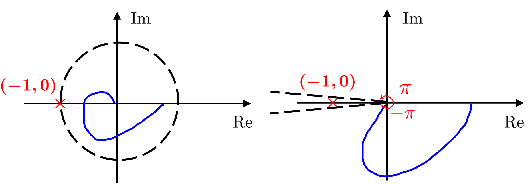
Figure 2: The region (left) from the small gain idea and the region (right) from the small phase idea for SISO Nyquist plots.

When MIMO subsystems are taken into consideration, we likewise aim at establishing the feedback stability from a gain or phase perspective as above based on the generalized Nyquist criterion [11, 12, 13] without any encirclement of “$-1$” made by the eigenloci of $P(s)$. To this end, one should first know what the notions of gain and phase are for a MIMO system. Over the past half-century, the research on gain-based theories, e.g., the small gain theorem [14] and $\mathcal{H}_{\infty}$ control theory [15, 16], has been flourishing [17, 18]. It is known that the gain of a stable MIMO LTI system represented by its frequency-response matrix is defined by the largest singular value $\overline{\sigma}(\cdot)$ of the matrix. Let $\lambda(\cdot)$ denote one of the eigenvalues of a matrix and $\lambda(P(j\omega))$ is referred to as the eigenloci of $P(s)$. The gain definition gives birth to the monumental small gain condition for a cyclic loop:

$$\left|\lambda(P(j\omega))\right|\leq\overline{\sigma}(P_{1}(j\omega))\overline{\sigma}(P_{2}(j\omega))\cdots\overline{\sigma}(P_{m}(j\omega))<1.$$

The condition above as an extension of the SISO gain case is also termed the product eigen-gain bound for matrices.

In comparison to the prosperous gain-based theory, the phase counterpart is however very much under-developed. For a long time there has even been a distinct lack of consensus on this counterpart among researchers. What is the phase of a matrix? What is the phase of a MIMO system? What is the formulation of a MIMO small phase theorem? These are the fundamental questions constantly asked by prominent control researchers in the 1980-1990s — various phasic notions were developed for different purposes, such as the “principal phase” [19], gain/phase integral relation [20, 21, 22], phase uncertainty [23, 24], and phase margin [25]. In addition, there were three qualitatively phase-related notions: the positive realness [26], negative imaginariness [27, 28, 29] and relaxation-type dynamics [30, 31, 32]. Very recently, these questions were also addressed with the thriving fruits upon the notion “sectorial phase” — on matrices [33, 34], MIMO LTI systems [35, 36, 37, 38, 39, 40], nonlinear systems [41, 42], and networks [43, 44]. In these references, the “sectorial phase” has shown its advantages in studying the feedback loop of two subsystems.

However, none of the existing phase notions above, to the best of our knowledge, are suitable for stability analysis of cyclic feedback systems with at least three components, i.e., $m\geq 3$. The crux of the issue lies in a lack of an appropriate matrix phase definition $\Psi(\cdot)$ having the following vital product eigen-phase bound for $m\geq 3$ matrices:

$$\angle{\lambda(P(j\omega))}\in\Psi(P_{1}(j\omega))+\cdots+\Psi(P_{m}(j\omega))\subset\interval[open]{-\pi}{\pi}.$$

Such a bound recovers the SISO phase case. More importantly, it acts as a significant enabling instrument in the formulation of a small phase theorem for a cyclic loop, analogously to the role of the product eigen-gain bound, as mentioned earlier, played in the small gain theorem.

Let us go deeper into two representative references [19, 36] in respect of the product eigen-phase bound. The pioneering work [19] proposes the “principal phase” of a matrix based on its polar decomposition. The product eigen-phase bound therein [19, Th. 2] only holds for one invertible matrix ($m=1$) provided that the spread of “principal phase” is less than $\pi$. This leads to an extra condition in the small “principal phase” result [19, (b) in Th. 4]. The recent paper [36] proposes the “sectorial phase” of a sectorial matrix based on the numerical range and sectorial decomposition. The product eigen-phase bound therein [36, Lem. 3] holds for two sectorial matrices, thereby leading to the successful small “sectorial phase” theorem [36, Th. 1] involving two sectorial subsystems. The theorem however cannot be extended to a cyclic loop with more than two components due to the intrinsic limitation of “sectorial phase”. Besides, studying only the sectorial-type of matrices/systems may be considered as another limitation.

Motivated in part by the importance of phase in classical control theory and by the pioneer “principal phase” and “sectorial phase” above, we expect an alternative notion of phase for matrices and MIMO systems having the product eigen-phase bound for any $m$ components, and then exploit this notion in stability analysis of cyclic feedback systems.

In this paper, we first propose a brand-new phase notion called the segmental phase for matrices and MIMO LTI systems. The proposed matrix segmental phase is graphically based on the normalized numerical range, a simply connected region contained in the unit disk, and is defined through the smallest circular segment of the disk covering the region. In particular, the matrix segmental phase has the crucial product eigen-phase bound as expected. We then formulate a small phase theorem for stability analysis of a cyclic loop involving semi-stable MIMO subsystems in Fig. 1, which requires the loop system phase to lie inside the $\interval[open]{-\pi}{\pi}$-cone, i.e., $\Psi(P_{1}(j\omega))+\cdots+\Psi(P_{m}(j\omega))\subset\interval[open]{-\pi}{\pi}$. The proposed theorem generalizes the classical SISO phase case and serves as a counterpart of the MIMO small gain theorem. Mixed small gain/phase theorems are further established for practical use via frequency-wise gain or phase conditions. Finally, a generalization of the small phase theorem is made by using angular scaling techniques for reducing conservatism, which is targeted at the scenario when the cyclic loop consists of known subsystems and phase-bounded uncertain subsystems simultaneously.

This paper has substantial differences and contributions beyond the authors’ conference paper [45] whose focal point lies on stable MIMO systems. The scope of the current paper covers more general subjects: The small phase theorem is now applicable to possibly semi-stable MIMO systems. Additionally, angular scaling techniques are proposed for reducing conservatism of the theorem, particularly suited for the case when some of subsystems in a cyclic loop are known.

The remainder of this paper is structured as follows. In Section II, we formulate the research problem: find a stability condition of cyclic feedback systems from a phasic viewpoint. In Section III, we define the segmental phase of a matrix based on the normalized numerical range. With the established mathematical underpinning, the segmental phase of a MIMO LTI system is developed in Section IV. Section V is dedicated to an LTI small phase theorem for stability analysis of cyclic feedback systems. For reducing conservatism, in Section VI a generalization of the proposed theorem is made and then a comparison is made between the segmental phase with the “sectorial phase”. Section VII concludes this paper.

Notation: The notation used in this paper is standard and will be made clear as we proceed. For two intervals $\interval{a}{b}$ and $\interval{c}{d}$ with $a\leq b$ and $c\leq d$, define the addition and subtraction as $\interval{a}{b}+\interval{c}{d}=\interval{a+c}{b+d}$ and $\interval{a}{b}-\interval{c}{d}=\interval{a-d}{b-c}$ by convention, respectively. The interval $[a,a]$ will be shortened as $a$ hereinafter without ambiguity. The argument of a complex number $z\in\mathbb{C}$ is denoted by $\angle z$, and $z$ has no argument if $z=0$. Let $\lambda_{i}(A)\in\mathbb{C}$ denote the $i$-th eigenvalue of a matrix $A\in{\mathbb{C}}^{n\times n}$, where $i=1,2,\ldots,n$, and $\overline{\sigma}(A)$ the largest singular value of $A$. Denote ${\mathbb{C}}_{+}$ and $\bar{\mathbb{C}}_{+}$ as the open and closed complex right half-plane, respectively. Denote by $\mathcal{R}^{n\times n}$ the set of $n\times n$ real-rational proper transfer function matrices. Denote $\mathcal{RH}_{\infty}^{n\times n}$ as the space consisting of $n\times n$ real-rational proper matrix-valued functions with no poles in $\bar{\mathbb{C}}_{+}$. A system $P(s)\in\mathcal{R}^{n\times n}$ is said to be semi-stable if it has no poles in ${\mathbb{C}}_{+}$; it is said to be stable if $G(s)\in\mathcal{RH}_{\infty}^{n\times n}$.

II Problem Formulation

Consider a cyclic feedback system shown in Fig. 1, where $P_{k}(s)\in\mathcal{R}^{n\times n}$ are MIMO systems, $e_{k}$ are external signals, and $u_{k}$ and $y_{k}$ are internal signals for $k=1,2,\ldots,m$. Denote $e\coloneqq\begin{bmatrix}e_{1}^{\top}&e_{2}^{\top}&\cdots&e_{m}^{\top}\end{bmatrix}^{\top}$ and $u\coloneqq\begin{bmatrix}u_{1}^{\top}&u_{2}^{\top}&\cdots&u_{m}^{\top}\end{bmatrix}^{\top}$. Our major interest is stability of the cyclic feedback system. The following definition of feedback stability mimics the standard definition of two open-loop systems in [16, Lem. 5.3].

Definition 1 (Cyclic feedback stability).

A cyclic feedback system in Fig. 1 is said to be stable if the following transfer function matrix (i.e., the mapping $e\mapsto u$):

$$\left[\begin{matrix}I&0&\cdots&0&P_{m}(s)\\ -P_{1}(s)&I&0&\cdots&0\\ \vdots&\ddots&\ddots&\ddots&\vdots\\ 0&\cdots&-P_{m-2}(s)&I&0\\ 0&\cdots&0&-P_{m-1}(s)&I\\ \end{matrix}\right]^{-1}$$ (1)

belongs to $\mathcal{RH}_{\infty}^{mn\times mn}$, where $I$ represents an appropriately dimensioned identity matrix.

In many applications, some of subsystems in Fig. 1 may not be precisely known and are oftentimes described by appropriate uncertain sets, while the remaining ones are assumed to be known. Robust control theory is targeted at such scenarios, where the monumental small gain theorem [14] has been one of the most important tools. A prerequisite for connecting the gain-based analysis to a feedback loop is to characterize uncertain systems by appropriate gain-bounded sets.

Denote by $\mathcal{B}_{\delta}$ the set of gain-bounded systems:

$$\mathcal{B}_{\delta}\coloneqq\left\{P(s)\in\mathcal{RH}_{\infty}^{n\times n}|~{}\overline{\sigma}(P(j\omega))\leq\delta(\omega),\omega\in\interval{0}{\infty}\right\},$$

where $\delta\colon\interval{0}{\infty}\to\interval[openright]{0}{\infty}$ represents a frequency-wise finite gain bound. Let $\mathcal{K}\subset\left\{1,2,\ldots,m\right\}$ denote the index set of uncertain systems in a cyclic loop. The set membership $k\in\left\{1,2,\ldots,m\right\}\setminus\mathcal{K}$ is hereinafter shortened as $k\notin\mathcal{K}$ without ambiguity. A direct application of the small gain theorem [16, Th. 9.1] yields the following feedback stability result.

Lemma 1.

Let $P_{1}(s),P_{2}(s),\ldots,P_{m}(s)\in\mathcal{RH}_{\infty}^{n\times n}$ and assume that $P_{k}(s)\in\mathcal{B}_{\delta_{k}}$ for $k\in\mathcal{K}$, where $\delta_{k}\colon\interval{0}{\infty}\to\interval[openright]{0}{\infty}$. The cyclic feedback system is stable if for all $\omega\in\interval{0}{\infty}$,

$$\prod_{k\in\mathcal{K}}\delta_{k}(\omega)\prod_{k\notin\mathcal{K}}\overline{\sigma}(P_{k}(j\omega))<1.$$ (2)

The gain-based condition (2) is composed of two parts. For those uncertain systems, their available information of gain bounds $\delta_{k}(\cdot)$ can only be adopted. For the remaining ones, their exact gains $\overline{\sigma}(\cdot)$ can be computed, and hence it becomes possible to reduce the conservatism of Lemma 1 via widely-adopted gain-scaling techniques (see [16, Ch. 11]).

We yearn for a parallel to the cyclic small gain theorem (Lemma 1) from a phasic perspective. To this end, we target at the following main problem:

Problem 1 (Feedback stability).

Consider $P_{1}(s),P_{2}(s),\ldots,$ $P_{m}(s)\in\mathcal{R}^{n\times n}$ and assume that $P_{k}(s)$ belongs to a certain set of “phase-bounded” uncertain systems for $k\in\mathcal{K}$. Find a phasic condition for stability of the cyclic feedback system.

For SISO LTI systems, the notion of phase is uncontroversial and thereby Problem 1 can be completely solved using the Nyquist stability criterion. For MIMO systems, Problem 1 is however quite nontrivial. To resolve this, our first need is an appropriate phase definition for MIMO systems, which has been recognized as a significant issue among several generations of control researchers [19, 23, 21, 20, 22, 24, 36]. The bottleneck behind the issue towards Problem 1 lies in the lack of a suitable matrix phase definition possessing the critical product eigen-phase bound, as pointed out in the introduction. This drives us to start with a simpler problem regarding to complex matrices.

Problem 2 (Matrix invertibility).

Find a phasic condition for invertibility of the matrix $I+A_{m}A_{m-1}\cdots A_{1}$, where $A_{1},A_{2},\ldots,A_{m}\in\mathbb{C}^{n\times n}$ with $A_{k}$ belongs to a certain set of “phase-bounded” uncertain matrices for $k\in\mathcal{K}$.

Solving Problem 2 serves as an intermediate but crucial step towards Problem 1 for frequency-domain analysis of MIMO systems in Section V. Our solution will be based on the development of a new phase definition for matrices and systems. To highlight the definition itself, for the time being let us assume that in Sections III-V all the matrices and systems under consideration are known, i.e., $\mathcal{K}=\emptyset$. We thus postpone the issue of uncertain components until Section VI in which Problems 1 and 2 will be completely resolved.

III The Segmental Phase of a Matrix

In this section, we establish a new matrix phase definition called the segmental phase, utilizing the normalized numerical phase of the matrix as studied in [46, 47]. The proposed definition yields the product eigen-phase bound, based on which a matrix small phase theorem is then obtained.

For a matrix $A\in{\mathbb{C}}^{n\times n}$, the normalized numerical range $\mathcal{N}(A)$ is defined by

$$\mathcal{N}(A)\coloneqq\left\{\frac{x^{*}Ax}{\left|x\right|\left|Ax\right|}\in\mathbb{C}\bigg{|}~{}0\neq x\in{\mathbb{C}}^{n},Ax\neq 0\right\},$$ (3)

where $\left|x\right|\coloneqq\sqrt{x^{*}x}$ and $x^{*}$ denote the Euclidean norm and the conjugate transpose of $x$, respectively. The normalized numerical range $\mathcal{N}(A)$ as a subset of a complex plane $\mathbb{C}$ is simply connected [47, Prop. 2.1]. By the Cauchy-Schwarz inequalities, $\mathcal{N}(A)$ is contained in the unit disk. Additionally, $\mathcal{N}(A)$ intersects with the unit circle only at the nonzero normalized eigenvalues of $A$, i.e., at $\frac{\lambda_{i}(A)}{\left|\lambda_{i}(A)\right|}$. A typical normalized numerical range is shown as the gray area in Fig. 3. Another quite obvious property of the normalized numerical range is that it is invariant to unitary similarity transformation, i.e., $\mathcal{N}(U^{*}AU)=\mathcal{N}(A)$ for every unitary matrix $U$.

Example 1.

The normalized numerical ranges of the following classes of matrices can be obtained easily.

1. If $A=ke^{j\alpha}I$, a scalar matrix, where $k>0$ and $\alpha\in\interval[openleft]{-\pi}{\pi}$, then $\mathcal{N}(A)$ is a singleton at $e^{j\alpha}$.

2. If $A$ is a positive definite matrix, then $\mathcal{N}(A)$ is a line segment connecting $\frac{2\sqrt{\kappa(A)}}{\kappa(A)+1}$ to $1$, where $\kappa(A)\coloneqq\frac{\overline{\lambda}(A)}{\underline{\lambda}(A)}$ denotes the condition number of $A$, shown in Fig. 4.

3. If $A$ is a unitary matrix, then $\mathcal{N}(A)$ is a polygon with the eigenvalues as vertices, also shown in Fig. 4.

4. If $A$ is a nonzero nilpotent Jordan block matrix, then $\mathcal{N}(A)$ is the whole open unit disk.

To dig up phase information of $A$ contained in $\mathcal{N}(A)$, we tailor a smallest circular segment, i.e., one with the shortest arc edge, of the unit disk to cover $\mathcal{N}(A)$ as shown in Fig. 3, the grey region $\mathcal{N}(A)$ is covered by the red-bordered circular segment. Then, we define the segmental phase $\Psi(A)$ of $A$ to be the following arc interval given by the circular segment:

$$\Psi(A)\coloneqq\interval{\underline{\psi}(A)}{\overline{\psi}(A)}$$ (4)

up to modulo $2\pi$. It holds that $\mathcal{N}(A)=\emptyset$ if and only if $A=0$, and thus a zero matrix $A$ has no phase $\Psi(A)=\emptyset$.

Two issues need to be further clarified. Firstly, a sector covering $\mathcal{N}(A)$ with the shortest arc edge is not necessarily unique, which makes the phase interval $\Psi(A)$ non-unique. One can easily construct a $n\times n$ unitary matrix $A$ with eigenvalues evenly distributed on the unit circle and hence $\mathcal{N}(A)$ being a regular polygon. In this case, the number of such smallest segments covering $\mathcal{N}(A)$ is exactly equal to $n$. Another extreme situation is when $A$ is a nonzero nilpotent Jordan matrix as in Example 1(iv). In this case, the smallest segment is given by the closed unit disk with one arbitrary boundary point excluded. Hence $\Psi(A)$ can be an arbitrary $2\pi$-interval. Notably, once the non-uniqueness exists, it implies that the length of the shortest arc is at least $\pi$.

Secondly, we allow the phase interval $\Psi(A)$ to be defined modulo $2\pi$, so it can be an interval in the whole real line. However, we often need to use the principal phase interval which is defined so that the phase center $\gamma^{\star}(A)=\frac{1}{2}\left(\underline{\psi}(A)+\overline{\psi}(A)\right)$ belongs to $(-\pi,\pi]$. Specifically, the general phase interval defined by $\Psi^{\mathrm{g}}(A)\coloneqq\Psi(A)+2\pi l$, where $l\in\mathbb{Z}$ is any integer, provides the most precise way of phase characterization. Nevertheless, we will not overly emphasize such a general definition hereafter.

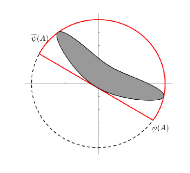
Figure 3: A graphical illustration of the segmental phase of $A=\left[-3+j4~{}1;0~{}{1}/(5+j)\right]$. The grey area is the normalized numerical range $\mathcal{N}(A)$ contained in the unit disk. The red-bordered smallest circular segment of the disk is adopted to cover $\mathcal{N}(A)$. This circular segment is characterized by the segmental phase $\Psi(A)=\interval{\underline{\psi}(A)}{\overline{\psi}(A)}=\interval[scaled]{\frac{-34.2\pi}{180}}{\frac{152.2\pi}{180}}$.

Note that $\angle\lambda_{i}(A)$ is also defined modulo $2\pi$. We can always find a $2\pi$-interval for $\angle\lambda_{i}(A)$ such that by the graphical definition (4), $\Psi(A)$ provides a bound of $\angle\lambda_{i}(A)$ from above and below, i.e., $\angle\lambda_{i}(A)\in\Psi(A)$. For some classes of matrices, the segmental phases have simple expressions in terms of eigenvalues as below.

Example 2.

We are to continue the case studies in Example 1.

1. If $A=ke^{j\alpha}I$, where $k>0$ and $\alpha\in\interval[openleft]{-\pi}{\pi}$, then $\gamma^{\star}(A)=\alpha$ and $\Psi(A)=\alpha$.

2. If $A$ is a positive definite matrix, then $\gamma^{\star}(A)=0$ and

   $$\Psi(A)=\textstyle\interval[scaled]{-\arccos\frac{2\sqrt{\kappa(A)}}{\kappa(A)+1}}{\arccos\frac{2\sqrt{\kappa(A)}}{\kappa(A)+1}}.$$

3. If $A$ is a unitary matrix, a longest side of it normalized numerical range divides the unit disk into two segments, one covering $\mathcal{N}(A)$ and one does not. The former is a smallest segment covering $\mathcal{N}(A)$ and its corners are two eigenvalues $e^{j\underline{\psi}}$ and $e^{j\overline{\psi}}$ of $A$ with a largest circular gap gives a definition of $\Psi(A)$. The segmental phase of $A$ can be defined as $\Psi(A)=[\underline{\psi},\overline{\psi}]$.

4. If $A$ is a nilpotent Jordan block matrix, then $\Psi(A)=[\gamma^{\star}(A)-\pi,\gamma^{\star}(A)+\pi]$, where $\gamma^{\star}(A)\in\interval[openleft]{-\pi}{\pi}$ is arbitrary.

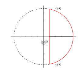
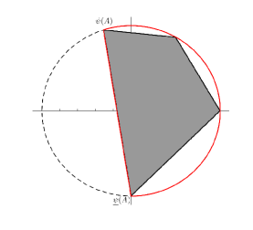
Figure 4: $\mathcal{N}(A)$ and $\Psi(A)$ for $A=\mathrm{diag}(1,20,100)$ (left, positive definite) and $A=\mathrm{diag}(-j,1,\frac{\pi}{3},\frac{3\pi}{5})$ (right, unitary).

We proceed to showing that the segmental phase is particularly useful in studying product of multiple matrices. The crucial product eigen-phase bound is elaborated as follows.

Theorem 1 (Product eigen-phase bound).

For $m$ matrices $A_{1},A_{2},\ldots,A_{m}\in{\mathbb{C}}^{n\times n}$, the arguments of the eigenvalues of $A_{m}A_{m-1}\cdots A_{1}$ can be chosen such that

$$\angle\lambda_{i}(A_{m}A_{m-1}\cdots A_{1})\in\Psi(A_{1})+\Psi(A_{2})+\cdots+\Psi(A_{m})$$

for $i=1,2,\ldots,n$, where $\lambda_{i}(A_{m}A_{m-1}\cdots A_{1})\neq 0$.

Proof:

See Appendix A. ∎

The full proof of Theorem 1 is provided in Appendix A, after we establish the connection between the segmental phase and the matrix singular angle [48, Sec. 23.5], an old but less known concept. The essential property showcased in Theorem 1 enables the use of the segmental phase in stability analysis of cyclic feedback systems and forms the nucleus of the phase study. Following immediately from Theorem 1, we can establish a cyclic small phase theorem for matrices as our first answer to the invertibility problem (Problem 2).

Theorem 2 (Matrix small phase theorem).

For $m$ matrices $A_{1},A_{2},\ldots,A_{m}\in{\mathbb{C}}^{n\times n}$, $I+A_{m}A_{m-1}\cdots A_{1}$ is invertible if

$$\sum_{k=1}^{m}\Psi(A_{k})\subset\interval[open]{-\pi}{\pi}.$$ (5)

Proof:

According to (5) and Theorem 1, it holds that

$${\angle\lambda_{i}(A_{m}A_{m-1}\cdots A_{1})}\in\sum_{k=1}^{m}\Psi(A_{k})\subset\interval[open]{-\pi}{\pi}$$

for $i=1,2,\ldots,n$, where $\lambda_{i}(A_{m}A_{m-1}\cdots A_{1})\neq 0$. This implies that $\det\left(I+A_{m}A_{m-1}\cdots A_{1}\right)\neq 0$ and $I+A_{m}A_{m-1}\cdots A_{1}$ is invertible. ∎

Equipped with the core matrix results, we are ready to cope with MIMO LTI systems via the newly-established notion of segmental phase.

IV The Segmental Phase of A MIMO LTI System

Let us begin with the celebrated notion of $\mathcal{H}_{\infty}$-norm [16, Sec. 4.3] of a stable MIMO LTI system $P(s)\in\mathcal{RH}_{\infty}^{n\times n}$:

$$\left\lVert P\right\rVert_{\infty}\coloneqq\sup_{\omega\in\interval{0}{\infty}}\overline{\sigma}(P(j\omega)).$$ (6)

Here, $\overline{\sigma}(P(j\omega))$, a continuous function of frequency $\omega$, is known as the system gain response (a.k.a. the frequency-wise gain). As a new counterpart to the gain, in this section we develop the phase response and $\mathcal{H}_{\infty}$-segmental-phase for a MIMO system based on the matrix segmental phase.

Unlike the gain definition restricted for stable systems, the phase definition below can apply to semi-stable systems which admit $j\omega$-axis poles. Additional notation on indented contours is required as follows before we move on.

IV-A The Indented Nyquist Contour and Preliminaries

Consider a semi-stable $P(s)\in\mathcal{R}^{n\times n}$ with full normal rank. Denote by ${\Omega}$ the set of nonnegative frequencies from the $j\omega$-axis poles of $P(s)$:

$${\Omega}\coloneqq\left\{\omega\in\interval[openright]{0}{\infty}|~{}s=j\omega~{}\text{is a pole of}~{}P(s)\right\}.$$

The unambiguous notation $j\Omega\coloneqq\left\{j\omega|~{}\omega\in\Omega\right\}$ and $j\Omega_{\pm}\coloneqq\left\{\pm j\omega|~{}\omega\in\Omega\right\}$ can also be adopted. Given $\omega_{0}\in\mathbb{R}$ and sufficiently small $\epsilon>0$, let $\mathbf{SC}(\epsilon,j\omega_{0})$ denote the following semi-circle in $\bar{\mathbb{C}}_{+}$ with the center $j\omega_{0}$ and radius $\epsilon$:

$$\mathbf{SC}(\epsilon,j\omega_{0})\coloneqq\left\{s\in\mathbb{C}|~{}\left|s-j\omega_{0}\right|=\epsilon,{\rm Re}\left(s\right)\geq 0\right\}.$$ (7)

Based on $\mathbf{SC}(\epsilon,j\omega_{0})$, define the indented Nyquist contour $\mathbf{NC}$ as depicted in Fig. 5. The contour $\mathbf{NC}$ has semicircular indentations with radius $\epsilon$ around $\pm j\omega_{0}$, where $\omega_{0}\in{\Omega}$. Define the leading coefficient matrix of $P(s)$ at a pole $j\omega_{0}\in j\Omega$ of order $l_{0}$ by

$${K(\omega_{0})}\coloneqq\lim_{s\to j\omega_{0}}{(s-j\omega_{0})^{l_{0}}}P(s).$$

Here, $K(\omega_{0})$ is a constant matrix with respect to $\omega_{0}$. For the sake of brevity, throughout this paper we consistently deal with the following set of semi-stable systems with full normal rank:

$$\mathcal{P}\coloneqq\left\{P(s)\in\mathcal{R}^{n\times n}|~{}P(s)~{}\text{is semi-stable with a set}~{}\Omega,\right.$$ (8)

$$\left.K(\omega_{0})~{}\text{has full rank for all}~{}\omega_{0}\in\Omega\right\}.$$

Note that the class $\mathcal{P}$ precludes those systems having $j\omega$-axis poles and zeros at the same locations.

Figure 5: An indented contour $\mathbf{NC}$ in $\bar{\mathbb{C}}_{+}$, where “$\times$” denotes the $j\omega$-axis poles and $\epsilon$ is taken to be sufficiently small.

We will exploit the frequency-response matrix $P(j\omega)$ to define the segmental phase of $P(s)$. When $P(s)$ has a pole at $s=j\omega_{0}$, an obvious difficulty arises for only considering $P(j\omega)$, since $P(j\omega_{0})$ is even not well defined. To handle the difficulty, we need the indented contour in Fig. 5 for determining possible phase changes of $P(j\omega)$ around the $j\omega$-axis poles. The same difficulty and treatment even exist in the SISO case when plotting the Bode phase diagram. The principle behind the treatment is more or less standard: As $\omega$ increases and $s$ travels around $\mathbf{SC}(\epsilon,j\omega_{0})$ counterclockwise, the certain “phase value” of $P(j\omega)$ should decrease by $l_{0}\pi$, where $j\omega_{0}$ is a pole of order $l_{0}$. For this reason, there is no ambiguity to determine a “phase value” of $P(j\omega)$ in the sense that the contour is always taken by convention. We refer the reader to [49, p. 93] for analogous consideration as above.

A similar story occurs around a $j\omega$-axis zero of $P(s)$, where intuitively a certain “phase value” should increase by that $\pi$ times the order of the zero. In comparison to the pole scenario, such a zero $j\omega_{0}$ is often easier to be handled, as the matrix $P(j\omega_{0})$ is well defined and so its “phase” supposed to be. The only trouble maker is any blocking zero, namely, $P(j\omega_{0})=0$, where a reasonable “phase value” should be empty at $j\omega_{0}$ causing allowable discontinuity. For the sake of brevity in our presentation, throughout we will not explicitly deal with “phase value” changes around $j\omega$-axis zeros. Nevertheless, keep in mind that a $j\omega$-axis-zeros-indented contour is inevitably required for determining appropriate “phase values” around those zeros.

IV-B The System Segmental Phase

Consider a semi-stable $P(s)\in\mathcal{P}$ defined in (8). We visualize the normalized numerical range $\mathcal{N}(P(j\omega))$, a frequency-dependent set continuous in $\omega\in\interval{0}{\infty}\setminus\Omega$ contained in the unit disk. Similarly to the matrix case in Fig. 3, graphically we tailor the frequency-dependent smallest circular segment to cover $\mathcal{N}(P(j\omega))$ for each $\omega\in\interval{0}{\infty}\setminus\Omega$. This immediately defines the (frequency-wise) segmental phase of $P(s)$:

$$\Psi(P(j\omega))\coloneqq\interval[scaled]{\underline{\psi}(P(j\omega))}{\overline{\psi}(P(j\omega))}$$ (9)

up to modulo $2\pi$, where $\omega\in\interval{0}{\infty}\setminus{\Omega}$. Note that $\Psi(P(j\omega))$ can also be termed as the system phase response.

A simple example of the system segmental phase is provided as follows for facilitating our graphical understanding. The new Bode-type phase response takes shape like a river whose two sides are exactly covered by $\overline{\psi}(P(j\omega))$ and $\underline{\psi}(P(j\omega))$.

Example 3.

Consider a $2\times 2$ system given by

$$P(s)=\frac{\begin{bmatrix}s^{3}+2s^{2}+3s+2&-2s-2\\ -3s-3&s^{3}+2s^{2}+6s+5\end{bmatrix}}{s^{4}+2s^{3}+8s^{2}+7s+4}.$$ (10)

The gain response and the newly defined phase response of $P(s)$ are depicted in Fig. 6 side-by-side which shares a similar flavor with the classical Bode diagram.

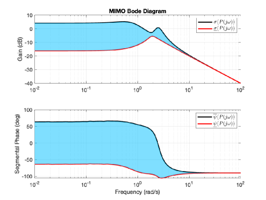
Figure 6: A complete MIMO Bode diagram of $P(s)$ in (10) over the frequency ranges $\interval{0.01}{100}~{}\textrm{rad/s}$. Top: the gain response $\interval{\underline{\sigma}(P(j\omega))}{\overline{\sigma}(P(j\omega))}$. Bottom: the newly defined phase response $\Psi(P(j\omega))=\interval[scaled]{\underline{\psi}(P(j\omega))}{\overline{\psi}(P(j\omega))}$.

Similarly to the matrix case, we should clarify several issues for an appropriate frequency-wise phase interval $\Psi(P(j\omega))$: principal values and non-uniqueness. Keep in mind that the interval-valued function $\Psi(P(j\omega))$ should shape like a “river”.

Firstly, determining a principal phase interval $\Psi(P(j\omega))$ demands specifying the principal phase center response $\gamma^{\star}(P(j\omega))$, i.e., the river’s center. The matrix principal phase center takes values in a fixed interval that is no longer suitable. To remedy this, let $\Gamma:\interval{0}{\infty}\to\mathbb{R}$ be piecewise continuous and make $\gamma^{\star}(P(j\omega))$ take values in $\Gamma(\omega)$. Then the principal phase interval $\Psi(P(j\omega))$ can be any suitable interval in the entire real line. Such a treatment is standard as also adopted in plotting Bode phase diagrams and in constructing Riemann surfaces [11] for system eigenloci.

Secondly, $\gamma^{\star}(P(j\omega))$ in general is not necessarily single valued and so is $\Psi(P(j\omega))$. Under the circumstances, we need to make a frequency-wise selection of $\gamma^{\star}(P(j\omega))$. Here is a guideline. As $\omega$ increases from $0$, we select one element from the set $\left\{\gamma^{\star}(P(j\omega))\right\}$ for each $\omega$ so as to make $\gamma^{\star}(P(j\omega))$ single-valued and meanwhile make $\Psi(P(j\omega))$ have a “continuous river flow” except for $\Omega\cup\Omega_{z}$, where $\Omega_{z}$ denotes the set of frequencies from $j\omega$-axis blocking zeros of $P(s)$. Such a selection is assumed throughout. Intuitively, the “river” should continuously carry water without interruptions.

Lastly, it remains to address $\Psi(P(j0))$ at the DC frequency $0$ as specifying the river’s source. If $0\notin\Omega$, $P(j0)$ is real and $\mathcal{N}(P(j0))$ is symmetric about the real axis. Without loss of generality (WLOG), assume that $\gamma^{\star}(P(j0))=0$. Since otherwise, “phase normalization” preprocessing for $P(s)$ can always be taken via multiplying $P(s)$ by some invertible $M\in\mathbb{R}^{n\times n}$ such that $\gamma^{\star}(P(j0)M)=0$. If $0\in\Omega$, the real matrix $P(\epsilon)$ is adopted instead and $\gamma^{\star}(P(\epsilon))=0$ is analogously assumed for sufficiently small $\epsilon>0$.

For facilitating the understanding of possibly non-unique phase responses and their selections, we provide an informative example as follows.

Example 4.

Consider $P(s)=\frac{A}{(s+j)(s-j)}$, where $A=\left[\begin{smallmatrix}0&1\\ -1&0\end{smallmatrix}\right]$. Then $P(j\omega)=\begin{bmatrix}0&\frac{1}{1-\omega^{2}}\\ -\frac{1}{1-\omega^{2}}&0\end{bmatrix}$, and $\mathcal{N}(P(j\omega))$ keeps the same region, the line segment connecting $-j$ to $j$, for all $\omega\in\interval[openright]{0}{1}\cup\interval[open]{1}{\infty}$, thereby having two possible matrix phase centers for each $\omega$, i.e., either $0$ or $\pi$. One should also recognize that a $\pi$-phase-shift occurs across the $j1$-pole by analyzing $\mathcal{N}(P(s))$ for $s\in\mathbf{SC}(\epsilon,j1)$. There are infinitely many candidates for $\Phi(P(j\omega))$, and among which an appropriate one can be selected to form a “river” according to the “continuous river flow” and phase center at $\omega=0$ guidelines. Concretely, the phase center $\gamma^{\star}(P(j0))=0$ is first selected to obtain $\Psi(P(j0))=\interval{-\frac{\pi}{2}}{\frac{\pi}{2}}$. Then we select

$$\Psi(P(j\omega))=\left\{\begin{aligned} &\textstyle\interval{-\frac{\pi}{2}}{\frac{\pi}{2}}\quad\quad\forall\omega\in\interval[open]{0}{1}\\ &\textstyle\interval{-\frac{3\pi}{2}}{-\frac{\pi}{2}}\quad\forall\omega\in\interval[open]{1}{\infty}.\end{aligned}\right.$$

Motivated by the $\mathcal{H}_{\infty}$-norm in (6), we next define the $\mathcal{H}_{\infty}$-segmental-phase of a semi-stable system $P(s)$ to be

$$\Psi_{\infty}(P)\coloneqq\interval[scaled]{\inf_{\omega\in\interval{0}{\infty}\setminus{\Omega}}\underline{\psi}(P(j\omega))}{\sup_{\omega\in\interval{0}{\infty}\setminus{\Omega}}\overline{\psi}(P(j\omega))}.$$ (11)

The interval $\Psi_{\infty}(P)$ consists of the minimum and maximum segmental phase of $P(s)$.

Note that the system segmental phases in (9) and (11) generalize the classical phase of semi-stable SISO LTI systems. To clarify this, let $G(s)\in\mathcal{R}^{1\times 1}$ be semi-stable. Straightforward calculation yields that

$$\Psi(G(j\omega))={\angle G(j\omega)}$$

for all $\omega\in\interval{0}{\infty}\setminus{\Omega}$. Moreover, one can observe that

$$\Psi_{\infty}(G)=\interval[scaled]{\inf_{\omega\in\interval{0}{\infty}\setminus{\Omega}}\angle G(j\omega)}{\sup_{\omega\in\interval{0}{\infty}\setminus{\Omega}}\angle G(j\omega)}$$

returns to the minimum and maximum classical phase of $G(s)$.

V Main Results: A Cyclic Small Phase Theorem

This section presents the main result of this paper, a cyclic small phase theorem, as a fundamental solution to the feedback stability Problem 1. The theorem states a brand-new stability condition involving the “loop system phase” being contained in $\interval[open]{-\pi}{\pi}$, and complements to the famous small gain theorem. Furthermore, a mixed small gain/phase theorem is established by intertwisting system gain/phase information in a frequency-wise manner.

Denote by $p_{k}$ the number of unstable poles (i.e., poles in $\bar{\mathbb{C}}_{+}$) of $P_{k}(s)$ for $k=1,2,\ldots,m$. A cyclic feedback system in Fig. 1 is said to have no unstable pole zero cancellation if the number of unstable poles of $P_{m}(s)P_{m-1}(s)\cdots P_{1}(s)$ is equal to $\sum_{k=1}^{m}p_{k}$. Throughout this paper, all cyclic feedback systems are reasonably assumed to be free of unstable pole-zero cancellations.

Consider a cyclic feedback system in Fig. 1, where subsystems $P_{k}(s)\in\mathcal{P}$ defined in (8) with $j\Omega_{k}$ for $k=1,2,\ldots,m$ and denote by $\Omega\coloneqq\bigcup_{k=1}^{m}\Omega_{k}$. We first state a technical assumption below that is needed to establish our main result later, whose role will be explained in details after that.

Assumption 1.

For each $\omega_{0}\in\Omega$, if any $P_{k}(s)$ satisfies that $\omega_{0}\notin\Omega_{k}$, $\Psi(P_{k}(j\omega))$ is unique and continuous at $\omega=\omega_{0}$.

For Assumption 1, considering that those $P_{k}(s)$ do not have poles at $s=j\omega_{0}$, verification of uniqueness and continuity of $\Psi(P_{k}(j\omega_{0}))$ is straightforward.

V-A A Cyclic Small Phase Theorem

Recall a simpler version of the small gain condition (2) for the cyclic feedback stability for all $P_{k}(s)\in\mathcal{RH}_{\infty}^{n\times n}$:

$$\prod_{k=1}^{m}\overline{\sigma}(P_{k}(j\omega))<1,$$ (12)

where $\omega\in\interval{0}{\infty}$. We are now ready for stating the main result, the so-called cyclic small phase theorem, which stands side-by-side with the small gain theorem. The result lays the foundation of the segmental phase study.

Theorem 3 (Cyclic small phase theorem).

Suppose that Assumption 1 holds. The cyclic feedback system is stable if

$$\sum_{k=1}^{m}\Psi(P_{k}(j\omega))\subset\interval[open]{-\pi}{\pi},$$ (13)

where $\omega\in\interval{0}{\infty}\setminus\Omega$.

Proof:

The full proof is postponed until Appendix D for the sake of readability. ∎

In Theorem 3, in the case of $P_{k}(s)\in\mathcal{RH}_{\infty}^{n\times n}$ for all $k=1,2,\ldots,m$, Assumption 1 is not needed and condition (13) requires to be examined for all $\omega\in\interval{0}{\infty}$. This reduces to [45, Th. 2] in our conference paper.

Let us now reveal the core messages enclosed in Theorem 3.

The small phase condition (13) involves a comparison of the sum of the phases (a.k.a. the loop-phase interval) to the interval $\interval[open]{-\pi}{\pi}$ in size. It is worthy of putting (12) and (13) into the context of the generalized Nyquist criterion [12] which underpins the proof of Theorem 3. The criterion counts the number of encirclements of the critical point “$-1$” made by the closed paths formed by the eigenloci of $P_{m}(s)P_{m-1}(s)\cdots P_{1}(s)$ when $s$ travels up the Nyquist contour. In the small gain case (12), the eigenloci are restricted in a simply connected region — the unit disk, so that there is no encirclement of “$-1$” and thereby the stability is guaranteed regardless of the arguments of the eigenloci. The small phase case (13) is developed in a parallel manner thanks to the vital product eigen-phase bound in Theorem 1. The eigenloci now are restricted in another simply connected region — the open $\interval[open]{-\pi}{\pi}$-cone so that the eigenloci never cross the negative real axis and thereby never encircle “$-1$”. Hence the stability is concluded regardless of the magnitudes of the eigenloci. Such an idea is graphical and intuitive.

The important idea of classical phase lead-lag compensation is naturally rooted in (13) which allows a phasic trade-off among all subsystems $P_{k}(s)$. In practice, some of subsystems may have large phase lags over certain frequency ranges. This can be compensated by the remaining ones with adequate phase leads over the same frequency ranges. Theorem 3 thus enables a loop-phase-shaping controller design problem via the segmental phase, and we leave it for future research.

Condition (13) suggests a robust-stability phase-indicator of a cyclic feedback loop. Specifically, the following quantity

$$\min_{\omega\in\interval{0}{\infty}\setminus\Omega}\;\pi-\max\left\{\left|\sum_{k=1}^{m}\overline{\psi}(P_{k}(j\omega))\right|,\left|\sum_{k=1}^{m}\underline{\psi}(P_{k}(j\omega))\right|\right\}$$ (14)

characterizes the worst case of “phase margin” of a cyclic loop over all positive constant scalings in the loop.

Two hidden technical ingredients of Theorem 3 need to be highlighted. Firstly, condition (13) is only examined for all $\omega\in\interval{0}{\infty}\setminus\Omega$. For every pole $j\omega_{0}\in j\Omega$ of order $l_{0}$, indent $j\mathbb{R}$ at $j\omega_{0}$ using a semi-circle $\mathbf{SC}(\epsilon,j\omega_{0})$. The proof of Theorem 3 claims the following: The fact that (13) holds for $s=j\omega$ and $\omega\in\interval{0}{\infty}\setminus\Omega$ implies that (13) also holds for all $s\in\mathbf{SC}(\epsilon,j\omega_{0})$. Assumption 1 plays a role in the claim, whose purpose is to technically guarantee that the loop-phase interval $\sum_{k=1}^{m}\Psi(P_{k}(s))$ entirely decreases by $l_{0}\pi$ when $s$ travels around $\mathbf{SC}(\epsilon,j\omega_{0})$ counterclockwise. In other words, except for $l_{0}\pi$, there is no other type of phase-value jumps around $s\in\mathbf{SC}(\epsilon,j\omega_{0})$ in the loop. Nevertheless, we anticipate that Theorem 3 still holds without the assumption.

Secondly, condition (13) together with Assumption 1 suggests that any pole $j\omega_{0}\in j\Omega$ must be at most of order $2$. This is although implicit but rather intuitive since we have seen that such a pole of order $l_{0}$ contributes a total $l_{0}\pi$-phase-decrease in the loop. If $l_{0}>2$, then clearly (13) does not hold. One may feel puzzled about $l_{0}=2$ since the total phase-shift around the pole seems to be already $2\pi$. In this case, note that the phase-shift may be an “open” rather than “closed” $2\pi$-decrease owing to potential lead-lag compensation among subsystems. An illustrative example is the feedback of a phase-lag $P_{1}(s)=\frac{\tau}{s^{2}}$ and a phase-lead $P_{2}(s)=\frac{s+1}{s+2}$, where $\tau>0$. Around $j0$, take $s=\epsilon e^{j\alpha}$ so that $P_{1}(s)=\tau\epsilon^{-2}e^{-j2\alpha}$ and $P_{2}(s)=\frac{1+\epsilon e^{j\alpha}}{2+\epsilon e^{j\alpha}}$. When $\alpha=-\frac{\pi}{2}$, $\angle P_{1}(-j\epsilon)=\pi$ for $\tau>0$. However, $P_{2}(-j\epsilon)=\frac{1-j\epsilon}{2-j\epsilon}$ provides a small phase-lag so that $\angle P_{1}(-j\epsilon)+\angle P_{2}(-j\epsilon)<\pi$ still holds for $\tau>0$. Similarly, when $\alpha=\frac{\pi}{2}$, we have $\angle P_{1}(j\epsilon)+\angle P_{2}(j\epsilon)>-\pi$ for $\tau>0$ by the conjugate symmetry of $P(j\omega)$.

The next corollary is developed in parallel to an $\mathcal{H}_{\infty}$-version of the small gain condition $\prod_{k=1}^{m}\left\lVert P_{k}\right\rVert_{\infty}<1$.

Corollary 1.

Suppose that Assumption 1 holds. The cyclic feedback system is stable if

$$\sum_{k=1}^{m}\Psi_{\infty}(P_{k})\subset\interval[open]{-\pi}{\pi}.$$

Proof:

The statement follows straightforwardly from definition (11) and Theorem 3. ∎

V-B Mixed Small Gain/Phase Theorems

In many applications, using gain or phase analysis alone may not meet our practical needs. Very often we should combine both of gain and phase information [50, Sec. 6.3], [19, 51, 52, 53, 54, 55, 38, 10, 56, 57]. A practical system usually has phase-lag increasing with input frequency and the phase shift for high frequency input is very much unknown and even undefined due to noise. In particular, a large number of control loops have components with large (or infinity) gains in the low frequencies and large (or undefined) phase lags in the high frequencies. The stability of such a loop can be established by applying the gain condition (12) to the high frequencies and the phase condition (13) to the low frequencies. This simple idea leads to the following mixed stability result.

Theorem 4.

Consider $P_{k}(s)\in\mathcal{P}$ with $\Omega_{k}$ satisfying that $\max_{\omega\in\Omega_{k}}\left|\omega\right|<\omega_{c}$ for $k=1,2,\ldots,m$, where $\omega_{c}\in\interval[open]{0}{\infty}$ is a given cut-off frequency. Suppose that Assumption 1 holds. The cyclic feedback system is stable if the following conditions hold:

1. $\displaystyle\sum_{k=1}^{m}\Psi(P_{k}(j\omega))\subset\interval[open]{-\pi}{\pi}$, where $\omega\in\interval[openright]{0}{\omega_{c}}\setminus\Omega;$

2. $\displaystyle\prod_{k=1}^{m}\overline{\sigma}(P_{k}(j\omega))<1$, where $\omega\in\interval{\omega_{c}}{\infty}$.

Proof:

The formal proof of Theorem 4 is omitted for brevity since it follows the similar lines of reasoning as those in the proof of Theorem 3. The main difference lies in that for high frequencies $\omega\in\interval{\omega_{c}}{\infty}$, we now have the eigenloci restricted in the unit disk, in contrast to the $\interval[open]{-\pi}{\pi}$-cone uniformly for all frequencies. ∎

The way of intertwisting gain/phase information using a cut-off frequency above is similar to that adopted in [19, Th. 5] and [38, Th. 1] where the control loop of two subsystems is concerned. Such an approach has also been utilized in combining gain/passivity information [51, 52, 56].

Theorem 4 can be further extended to a frequency-wise mixed gain/phase version. The idea is intuitive: at each frequency, a gain condition or a phase condition is applied. It can be well understood via the Nyquist idea [12]: The eigenloci are contained in the set union of the unit disk and $\interval[open]{-\pi}{\pi}$-cone — a new simply connected region away from “$-1$”.

Theorem 5 (Mixed gain/phase theorem).

Suppose that Assumption 1 holds. The cyclic feedback system is stable if for each $\omega\in\interval{0}{\infty}\setminus\Omega$, one of the following conditions holds:

1. $\displaystyle\sum_{k=1}^{m}\Psi(P_{k}(j\omega))\subset\interval[open]{-\pi}{\pi};$

2. $\displaystyle\prod_{k=1}^{m}\overline{\sigma}(P_{k}(j\omega))<1$.

Proof:

The full proof is omitted. It follows the similar lines of reasoning as those in the proof of Theorem 3 by using the set union of the unit disk and $\interval[open]{-\pi}{\pi}$-cone. In such a case, all the eigenloci $\lambda_{i}(P(s))\in\mathcal{D}$ for all $s$ in the contour $\mathbf{NC}$ and $i=1,2,\ldots,n$, where $P(s)=P_{m}(s)P_{m-1}(s)\cdots P_{1}(s)$ and $\mathcal{D}\coloneqq\left\{z\in\mathbb{C}|~{}\left|z\right|<1~{}\text{or}~{}\angle z\in\interval[open]{-\pi}{\pi}\right\}$. ∎

In Theorem 5, it is worth noting that for those frequencies $\omega$ arbitrarily close to an element in $\Omega$, i.e., around a pole, the gain condition (ii) is impossible to be fulfilled, and only the phase condition (i) is possible to be applied to the frequencies.

VI A Generalized Cyclic Small Phase Theorem

The purpose of this section is twofold. First, in the stability problem (Problem 1), considering that some of subsystems are known in advance, we propose to introduce angular scaling techniques to fully use the known information. In particular, an angular scaling function $\gamma$, referred to as the $\gamma$-segmental phase, can be tailored for each known subsystem. This leads to a generalized cyclic small phase theorem. Second, equipped with the $\gamma$-segmental phase, we extend applicability of our study which incorporates the recent sectorial phase [36].

We seek an answer to the invertibility problem (Problem 2) first and remind the reader that $\mathcal{K}$ represents the index set of uncertain matrices/systems.

VI-A The Matrix $\gamma$-Segmental Phase

The matrix segmental phase (4) implicitly contains the phase center $\gamma^{\star}(A)$ optimal for a given $A$. In Problem 2, when invertibility of $I+A_{m}A_{m-1}\cdots A_{1}$ is concerned, where $A_{k}$ or $\mathcal{N}(A_{k})$ is known for $k\notin\mathcal{K}$, each independent phase center $\gamma^{\star}(A_{k})$ for $k\notin\mathcal{K}$ however can bring conservatism in determining the invertibility. One natural approach of reducing such the conservatism is to allow a jointly design of “new centers” for those known matrices. To achieve this, we propose an adjustable inclined center $\gamma$ for a matrix as an angular scaling parameter.

Given a matrix $A\in{\mathbb{C}}^{n\times n}$ with $\mathcal{N}(A)$, we associate $A$ with a parameter $\gamma$, where $\gamma\in\interval[openleft]{-\pi}{\pi}$. Graphically we tailor the smallest circular segment with respect to the inclined center $\gamma$ to cover $\mathcal{N}(A)$. The $\gamma$-segmental phase $\Psi_{\gamma}(A)$ of $A$ is defined as the following arc interval given by the segment:

$$\Psi_{\gamma}(A)\coloneqq\interval[scaled]{\underline{\psi}_{\gamma}(A)}{\overline{\psi}_{\gamma}(A)}$$ (15)

up to modulo $2\pi$. As illustrated by Fig. 7, the grey region $\mathcal{N}(A)$ is covered by the green-bordered circular segment with respect to the inclined center $\gamma$.

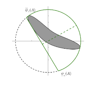
Figure 7: An illustration of $\Psi_{\gamma}(A)=\interval{\frac{-71.7\pi}{180}}{\frac{131.7\pi}{180}}$ with respect to the inclined center $\gamma=\frac{\pi}{6}$ for the same $A$ in Fig. 3.

An obvious graphical difference exists between the segmental phase $\Psi(A)$ and $\gamma$-segmental phase $\Psi_{\gamma}(A)$. The latter depends on the parameter $\gamma$, and thereby in (15) the segment for covering $\mathcal{N}(A)$ always has the center $\gamma$ (or lies with the slope $\tan\gamma$). In particular, as a special case when $\gamma$ is chosen to be $\gamma^{\star}(A)$ in (4), $\Psi_{\gamma}(A)$ then recovers to $\Psi(A)$.

It is time to revisit Problem 2. It is worth noting that the different roles of $\Psi(A)$ and $\Psi_{\gamma}(A)$ can be played in Problem 2. The former is used to characterize phase-bounded uncertain sets, analogously to the singular value for gain-bounded sets. The later is considered as angular-scaling techniques for known matrices, similarly to gain-scaling ideas.

Denote by $\mathcal{A}_{\interval{\alpha}{\beta}}$ the set of phase-bounded matrices:

$$\mathcal{A}_{\interval{\alpha}{\beta}}\coloneqq\left\{A\in{\mathbb{C}}^{n\times n}|~{}\Psi(A)\subset\interval{\alpha}{\beta},\beta-\alpha\in\interval[openright]{0}{2\pi}\right\}.$$

For $k\in\mathcal{K}$, assume that $A_{k}\in\mathcal{A}_{\interval{\alpha_{k}}{\beta_{k}}}$; for $k\notin\mathcal{K}$, adopt $\Psi_{\gamma_{k}}(A_{k})$ by embedding a parameter $\gamma_{k}$ to be designed respectively. The following toy example facilitates the motivation of the use of $\Psi_{\gamma_{k}}(A_{k})$ in Problem 2.

Example 5.

Consider $2\times 2$ matrices $A_{1}=A_{2}=e^{j\frac{\pi}{3}}B$ and $A_{3}\in\mathcal{A}_{\interval{-\frac{\pi}{2}}{\frac{\pi}{2}}}$, where $B=\mathrm{diag}\left(1,3\right)$ is positive definite with the condition number $\kappa(B)=3$. Clearly, for $k=1,2$, $\mathcal{N}(A_{k})$ is a rotated line segment and it follows from Example 2(ii) that $\Psi(A_{k})=\interval[scaled]{0}{\frac{\pi}{3}}$. Since $A_{3}$ is uncertain, the worst case is given by $\sum_{k=1}^{3}\overline{\psi}(A_{k})=\frac{7\pi}{6}$ and thereby Theorem 2 is not satisfied. However, one can choose $\gamma_{1}=\gamma_{2}=0$ and by some calculations we obtain that

$$\sum_{k=1}^{2}\Psi_{\gamma_{k}}(A_{k})+\Psi(A_{3})\subset\textstyle\interval{-\frac{172.82\pi}{180}}{\frac{172.82\pi}{180}}\subset\interval[open]{-\pi}{\pi}.$$

Clearly, a “generalized” small phase condition can be satisfied thanks to $\gamma$-segmental phases.

The idea distilled from Example 5 can be rigorously formulated into the following theorem specific to Problem 2.

Theorem 6.

For $m$ matrices $A_{1},A_{2},\ldots,A_{m}\in{\mathbb{C}}^{n\times n}$, suppose that $A_{k}\in\mathcal{A}_{\interval{\alpha_{k}}{\beta_{k}}}$ for $k\in\mathcal{K}$. Then $I+A_{m}A_{m-1}\cdots A_{1}$ is invertible if there exist $\gamma_{k}\in\interval[openleft]{-\pi}{\pi}$ for $k\notin\mathcal{K}$ such that

$$\sum_{k\notin\mathcal{K}}\Psi_{\gamma_{k}}(A_{k})+\sum_{k\in\mathcal{K}}\interval{\alpha_{k}}{\beta_{k}}\subset\interval[open]{-\pi}{\pi}.$$ (16)

Proof:

See Appendix B. ∎

Theorem 6 unifies the segmental phase and $\gamma$-segmental phase into one condition (16). The searching of feasible $\gamma_{k}$ in (16) can be formulated as a nonlinear optimization problem and we note this for further research.

VI-B A Generalized Cyclic Small Phase Theorem

We are ready to revisit Problem 1 and can apply the core idea extracted from Theorem 6 to feedback stability analysis.

Let $\mathcal{S}_{\interval{\alpha}{\beta}}$ denote the following set of phase-bounded uncertain stable systems:

$$\mathcal{S}_{\interval{\alpha}{\beta}}\coloneqq\left\{P(s)\in\mathcal{RH}_{\infty}^{n\times n}|~{}\Psi(P(j\omega))\subset\interval{\alpha(\omega)}{\beta(\omega)},\right.\\ \left.\text{where}~{}\omega\in\interval{0}{\infty}\setminus\Omega~{}\text{and}~{}\beta(\omega)-\alpha(\omega)\in\interval[openright]{0}{2\pi}\right\},$$

where $\alpha:\interval{0}{\infty}\to\mathbb{R}$ and $\beta\colon\interval{0}{\infty}\to\mathbb{R}$ jointly characterize a frequency-wise phase bound. Consider a cyclic loop, where $P_{k}(s)\in\mathcal{S}_{\interval{\alpha}{\beta}}$ for $k\in\mathcal{K}$ and $P_{k}(s)\in\mathcal{P}$ in (8) for $k\notin\mathcal{K}$.

We now associate $P_{k}(j\omega)$ for $k\notin\mathcal{K}$ with a frequency-wise inclined center $\gamma_{k}(\omega)$. Denote by $\Omega={\bigcup_{k\notin\mathcal{K}}\Omega_{k}}$ and consider the following set of scalar functions for $P_{k}(s)$:

$$\mathcal{F}_{k}\coloneqq\left\{\gamma_{k}:\interval{0}{\infty}\to\mathbb{R}|~{}\gamma_{k}(\omega)~{}\text{is piecewise continuous};\right.\\ \left.\gamma_{k}(\omega)~{}\text{is continuous for}~{}\omega\in{\Omega\setminus\Omega_{k}}\right\}.$$ (17)

For a semi-stable $P_{k}(s)$, the set $\mathcal{F}_{k}$ is rather general although requiring a mild condition of continuity at $\omega\in\Omega\setminus\Omega_{k}$. The purpose of the continuity is to assure that when $\omega\in\Omega\setminus\Omega_{k}$, i.e., the frequencies that other subsystems having poles, no extra phase-value jump can be caused from $\mathcal{F}_{k}$ for $P_{k}(s)$.

Here comes our second feedback stability result to Problem 1, a generalized cyclic small phase theorem.

Theorem 7 (Generalized small phase theorem).

Suppose that Assumption 1 holds. The cyclic feedback system is stable if there exist functions $\gamma_{k}(\omega)\in\mathcal{F}_{k}$ for $k\notin\mathcal{K}$ such that

$$\sum_{k\notin\mathcal{K}}\Psi_{\gamma_{k}(\omega)}(P_{k}(j\omega))+\sum_{k\in\mathcal{K}}\interval{\alpha_{k}(\omega)}{\beta_{k}(\omega)}\subset\interval[open]{-\pi}{\pi}$$ (18)

holds for $\omega\in\interval{0}{\infty}\setminus\Omega$.

Proof:

See Appendix D. ∎

For the sake of readability, the proof of Theorem 7 is postponed whose main idea is again based on a Nyquist approach. There is a notable correspondence between Theorem 7 (phase) and Lemma 1 (gain) for uncertain cyclic feedback systems.

Searching appropriate $\gamma_{k}(\omega)$ in (18) is a frequency-sweep test and how to efficiently solve $\gamma_{k}(\omega)$ remains nontrivial and is our ongoing research. For example, motivated by the worst case of “phase margin” characterized in (14), we can formulate a max-min design problem for $\gamma_{k}(\omega)$ to improve the worst “phase margin” in line with (18).

VI-C Relation with the Recent Sectorial Phase

In this subsection, we link the segmental phase to the recent sectorial phase [36]. Their most intuitive difference is clarified from a graphical point of view. We then show that the sectorial small phase theorem [36] can be subsumed into Theorem 7.

Some preliminaries on the matrix sectorial phase are needed. A matrix $A\in{\mathbb{C}}^{n\times n}$ is said to be sectorial if the normalized numerical range $\mathcal{N}(A)$ does not contain the origin and is contained in an open half-plane. For a sectorial $A$, there are two unique supporting rays of $\mathcal{N}(A)$ to form a convex circular sector anchored at the origin, and thus the opening angle of this sector is strictly less than $\pi$. Then the sectorial phase of a sectorial matrix $A$ is defined by

$$\Phi_{\textrm{sect}}(A)\coloneqq\interval[scaled]{\inf_{0\neq z\in\mathcal{N}(A)}\angle z}{\sup_{0\neq z\in\mathcal{N}(A)}\angle z}.$$

See a graphical illustration of the sectorial phase in Fig. 8. The two terms “segmental phase” and “sectorial phase” signify their first and biggest difference vividly. The former exploits the smallest segment to bound $\mathcal{N}(A)$, while the latter adopts the smallest convex sector. Besides, the two notions differ in a few other significant aspects. The segmental phase is defined for all matrices, but the sectorial phase is subject to the class of “sectorial matrices”. The former has the product eigen-phase bound for multiple matrices, while the latter only has such a bound for at most two sectorial matrices [33].

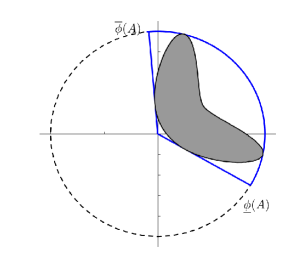
Figure 8: An illustration of the sectorial phase of a sectorial matrix $A\in\mathbb{C}^{2\times 2}$. The blue-bordered smallest convex circular cone is adopted to bound $\mathcal{N}(A)$.

Our framework can incorporate the framework of the matrix and system sectorial phases. The following corollary rephrases the matrix sectorial small phase theorem [36], and an alternative proof can be provided based on Theorem 6.

Corollary 2 ([36, Lem. 2.5]).

For sectorial matrices $A_{1},A_{2}\in{\mathbb{C}}^{n\times n}$, the matrix $I+A_{2}A_{1}$ is invertible if

$$\Phi_{\emph{{sect}}}(A_{1})+\Phi_{\emph{{sect}}}(A_{2})\subset\interval[open]{-\pi}{\pi}.$$ (19)

Proof:

According to condition (19), there exists a common $\alpha\in\interval[openleft]{-\pi}{\pi}$ such that $e^{-j\alpha}\mathcal{N}(A_{1})=\mathcal{N}\left(e^{-j\alpha}A_{1}\right)\subset{\mathbb{C}}_{+}$ and $e^{j\alpha}\mathcal{N}(A_{2})=\mathcal{N}\left(e^{j\alpha}A_{2}\right)\subset{\mathbb{C}}_{+}$; namely, $\mathcal{N}(A_{1})$ and $\mathcal{N}(A_{2})$ can be rotated into ${\mathbb{C}}_{+}$ simultaneously. It follows that

$$\theta\left(e^{-j\alpha}A_{1}\right)<\pi/2~{}\text{and}~{}\theta\left(e^{j\alpha}A_{2}\right)<\pi/2,$$ (20)

where $\theta(\cdot)$ is specified in (21). Choose $\gamma_{1}=\alpha$ and $\gamma_{2}=-\alpha$ and adopt them as the $\gamma$-segmental phases for $A_{1}$ and $A_{2}$, respectively. By definition (15) with an expression (26) in Appendix B, we have

$$\overline{\psi}_{\gamma_{1}}(A_{1})+\overline{\psi}_{\gamma_{2}}(A_{2}) =\alpha+\theta\left(e^{-j\alpha}A_{1}\right)-\alpha+\theta\left(e^{j\alpha}A_{2}\right),$$

$$\underline{\psi}_{\gamma_{1}}(A_{1})+\underline{\psi}_{\gamma_{2}}(A_{2}) =\alpha-\theta\left(e^{-j\alpha}A_{1}\right)-\alpha-\theta\left(e^{j\alpha}A_{2}\right),$$

This gives that $\Psi_{\gamma_{1}}(A_{1})+\Psi_{\gamma_{2}}(A_{2})\subset\interval[open]{-\pi}{\pi}$ by (20). The proof is finished by invoking Theorem 6 with $\mathcal{K}=\emptyset$. ∎

A take-away message behind Corollary 2 is that the sectorial condition (19) implies the existence of a pair of complementary angular scaling, i.e., $e^{-j\alpha}$ for $A_{1}$ and $e^{j\alpha}$ for $A_{2}$, such that $\mathcal{N}(A_{1})$ and $\mathcal{N}(A_{2})$ can be rotated into ${\mathbb{C}}_{+}$ simultaneously.

Feedback stability analysis via the sectorial phase can similarly be recovered by $\gamma$-segmental phases. Specifically, $P(s)\in\mathcal{RH}_{\infty}^{n\times n}$ is said to be frequency-wise sectorial [36, Sec. 3] if $P(j\omega)$ is sectorial for all $\omega\in\interval{0}{\infty}$. The following LTI sectorial small phase theorem [36] is re-established by Theorem 7 as a corollary.

Corollary 3 ([36, Th. 4.1]).

Let $P_{1}(s),P_{2}(s)\in\mathcal{RH}_{\infty}^{n\times n}$ be frequency-wise sectorial. The feedback system is stable if

$$\Phi_{\emph{{sect}}}(P_{1}(j\omega))+\Phi_{\emph{{sect}}}(P_{2}(j\omega))\subset\interval[open]{-\pi}{\pi}\quad\forall\omega\in\interval{0}{\infty}.$$

Proof:

By hypothesis, there exists a continuous conjugate symmetric function $\alpha:\interval{-\infty}{\infty}\to\mathbb{C}$, i.e., $\alpha(x)=\overline{\alpha(-x)}$ for all $x\in\interval{-\infty}{\infty}$, such that for all $\omega\in\interval{0}{\infty}$, we have $\mathcal{N}\left(e^{-j\angle\alpha(\omega)}P_{1}(j\omega)\right)\subset{\mathbb{C}}_{+}$ and $\mathcal{N}\left(e^{j\angle\alpha(\omega)}P_{2}(j\omega)\right)\subset{\mathbb{C}}_{+}$. This implies that for all $\omega\in\interval{0}{\infty}$, we have

$$\theta\left(e^{-j\angle\alpha(\omega)}P_{1}(j\omega)\right)<\pi/2~{}\text{and}~{}\theta\left(e^{j\angle\alpha(\omega)}P_{2}(j\omega)\right)<\pi/2.$$

We tailor the $\gamma$-segmental phases for $P_{1}(s)$ and $P_{2}(s)$. Choosing $\gamma_{1}(j\omega)=\angle\alpha(\omega)$ and $\gamma_{2}(j\omega)=-\angle\alpha(\omega)$ yields that

$$\overline{\psi}_{\gamma_{1}(j\omega)}(P_{1}( j\omega))+\overline{\psi}_{\gamma_{2}(j\omega)}(P_{2}(j\omega))$$

$$=\left(e^{-j\angle\alpha(\omega)}P_{1}(j\omega)\right)+\theta\left(e^{j\angle\alpha(\omega)}P_{2}(j\omega)\right),$$

$$\underline{\psi}_{\gamma_{1}(j\omega)}(P_{1}( j\omega))+\underline{\psi}_{\gamma_{2}(j\omega)}(P_{2}(j\omega))$$

$$=-\theta\left(e^{-j\angle\alpha(\omega)}P_{1}(j\omega)\right)-\theta\left(e^{j\angle\alpha(\omega)}P_{2}(j\omega)\right)$$

for all $\omega\in\interval{0}{\infty}$. It follows that $\Phi_{\gamma_{1}(j\omega)}(P_{1}(j\omega))+\Phi_{\gamma_{2}(j\omega)}(P_{2}(j\omega))\subset\interval[open]{-\pi}{\pi}$ for all $\omega\in\interval{0}{\infty}$. The proof is completed due to Theorem 7 by setting $\mathcal{K}=\emptyset$. ∎

Only stable and sectorial systems are under consideration in Corollary 3 for the sake of brevity, although [36] also studies the sectorial phase of a general class of systems — semi-stable and semi-sectorial systems. It is worth noting that Theorem 7 can also cover the generalized result [36, Th. 7.1] since Theorem 7 admits semi-stable systems likewise. Showing this will be technically cumbersome requiring additional definitions for the sectorial phase, but follows the similar lines of reasoning in the proof of Corollary 3 and is thus omitted.

VII Conclusion

In this paper, we first propose the segmental phase of matrices and MIMO LTI systems. The segmental phase has the important product eigen-phase bound and acts as a new counterpart to the gain notion. Based on the segmental phase, we then establish a small phase theorem for stability analysis of cyclic feedback systems with multiple subsystems, which stands side-by-side with the small gain theorem. When some of subsystems in the loop are known, we further propose the $\gamma$-segmental phase and develop a generalized cyclic small phase theorem to reduce the conservatism. Finally, we demonstrate that feedback stability analysis via the recent sectorial phase can be subsumed into our proposed framework.

Extensions of the segmental phase to nonlinear and time-varying systems and the computation of segmental phases are under investigation. Other future research directions embrace counterparts of $\mathcal{H}_{\infty}$-controller synthesis methods via the segmental phase. It is hoped that this paper offers a brand-new viewpoint for the recent renaissance of phase in the field of systems and control.

Appendix A The Segmental Phase Behind the Scenes

The purpose of this appendix is to facilitate the understanding of the segmental phase by establishing an important connection with the matrix singular angle and some optimization formulations. After having these preparations, we provide the full proof of Theorem 1.

A-A The Matrix Case

We first present some preliminaries on the notion of matrix singular angle [48, Sec. 23] which is an old but less known concept. For a matrix $A\in\mathbb{C}^{n\times n}$, the singular angle $\theta(A)\in\interval{0}{\pi}$ is defined by

$$\theta(A)\coloneqq\displaystyle\sup_{\begin{subarray}{c}0\neq x\in\mathbb{C}^{n},\\ {Ax}\neq 0\end{subarray}}\arccos\frac{{\rm Re}\left(x^{*}Ax\right)}{\left|x\right|\left|Ax\right|},$$ (21)

where ${\rm Re}\left(\cdot\right)$ represents the real part of a scalar. By exploiting the normalized numerical range $\mathcal{N}(A)$ in (3), we reformulate definition (21) as follows: $\theta(A)=\sup_{z\in\mathcal{N}(A)}\arccos{\rm Re}\left(z\right)$. The singular angle has two useful properties as detailed in the following two lemmas.

Lemma 2 ([48, Sec. 23.5]).

For a matrix $A\in{\mathbb{C}}^{n\times n}$, it holds that $\left|\angle\lambda_{i}(A)\right|\leq\theta(A)$ for $i=1,2,\ldots,n$, where $\lambda_{i}(A)\neq 0$.

Lemma 3 ([48, Sec. 23.5]).

For matrices $A$, $B\in\mathbb{C}^{n\times n}$, it holds that $\theta(AB)\leq\theta(A)+\theta(B)$.

Equipped with the singular angle, we then establish an algebraic expression of the segmental phase defined in (4). For $A\in{\mathbb{C}}^{n\times n}$, the phase center $\gamma^{\star}(A)\in\interval[openleft]{-\pi}{\pi}$ of $A$ can be expressed through the following optimization problem:

$$\gamma^{\star}(A)=\arg\min_{\gamma\in\interval[openleft]{-\pi}{\pi}}\theta\left(e^{-j\gamma}A\right)$$

and $r^{\star}(A)\coloneqq\theta\left(e^{-j\gamma^{\star}(A)}A\right)\in\interval{0}{\pi}$ is termed the phase radius of $A$. The segmental phase of $A$ can be represented by

$$\Psi(A)=\interval{\underline{\psi}(A)}{\overline{\psi}(A)},$$

where

$$\overline{\psi}(A) =\gamma^{\star}(A)+r^{\star}(A)$$ (22)

$$\underline{\psi}(A) =\gamma^{\star}(A)-r^{\star}(A).$$

The phase radius $r^{\star}(A)$ is used to characterize the spread of the smallest segment in Fig. 3, i.e., $\overline{\psi}(A)-\underline{\psi}(A)=2r^{\star}(A)$, which has an analogy to the condition number $\kappa(A)=\frac{\overline{\sigma}(A)}{\underline{\sigma}(A)}$. In particular, for a positive definite matrix $A$, $r^{\star}(A)$ and $\kappa(A)$ are closely connected as stated in Example 2(ii).

Based on the connections, we are ready to prove Theorem 1.

Proof:

For the notational simplicity, let $\gamma_{k}^{\star}\coloneqq\gamma^{\star}(A_{k})$ for $k=1,2,\ldots,m$ and $A\coloneqq A_{m}A_{m-1}\cdots A_{1}$. WLOG, suppose that $\Psi(A_{1})+\Psi(A_{2})+\cdots+\Psi(A_{m})$ is contained in an open $2\pi$-interval $\interval[open]{\alpha-\pi}{\alpha+\pi}$, where $\alpha\in\mathbb{R}$, since otherwise the statement trivially holds for $\angle\lambda_{i}(A)$. In addition, notice that $\angle\lambda_{i}(A)$ can be chosen modulo $2\pi$.

By hypothesis and using (22), we have that

$$\textstyle\sum_{k=1}^{m}\gamma_{k}^{\star}+\theta\left(e^{-j\gamma_{k}^{\star}}A_{k}\right) <\alpha+\pi$$

$$\textstyle\sum_{k=1}^{m}\gamma_{k}^{\star}-\theta\left(e^{-j\gamma_{k}^{\star}}A_{k}\right) >\alpha-\pi.$$

Since $\theta\left(e^{-j\gamma_{k}^{\star}}A_{k}\right)\geq 0$ for all $k=1,2,\ldots,m$, it follows that $\textstyle\sum_{k=1}^{m}\gamma_{k}^{\star}\in\interval[open]{\alpha-\pi}{\alpha+\pi}$. Note that for arbitrary $\gamma\in\interval[open]{\alpha-\pi}{\alpha+\pi}$, it holds that

$$\angle\lambda_{i}(A)-\gamma=\angle\lambda_{i}\left(e^{-j\gamma}A\right)\mod 2\pi$$ (23)

for $\lambda_{i}(A)\neq 0$ and $i=1,2,\ldots,n$. In addition, according to Lemma 2, we have that

$$\left|\angle\lambda_{i}\left(e^{-j\gamma}A\right)\right|\leq\theta\left(e^{-j\gamma}A\right)$$ (24)

for $\lambda_{i}(A)\neq 0$ and $i=1,2,\ldots,n$. Combining (23) and (24) and substituting $\gamma=\sum_{k=1}^{m}\gamma_{k}^{\star}$ into them yield that

$$\textstyle\left|\angle\lambda_{i}(A)-\sum_{k=1}^{m}\gamma_{k}^{\star}\right| \leq\theta\left(e^{-j{\sum_{k=1}^{m}\gamma_{k}^{\star}}}A\right)$$

$$=\theta\left(e^{-j{\gamma_{1}^{\star}}}A_{1}e^{-j{\gamma_{2}^{\star}}}A_{2}\cdots e^{-j{\gamma_{m}^{\star}}}A_{m}\right)$$

$$\leq\sum_{k=1}^{m}\theta\left(e^{-j\gamma^{\star}_{k}}A_{k}\right)$$

for $\lambda_{i}(A)\neq 0$ and $i=1,2,\ldots,n$, where the last inequality uses Lemma 3. This implies that

$$\textstyle\sum_{k=1}^{m}\gamma_{k}^{\star}-\theta\left(e^{-j\gamma_{k}^{\star}}A_{k}\right)\leq\angle\lambda_{i}(A)\leq\sum_{k=1}^{m}\gamma_{k}^{\star}+\theta\left(e^{-j\gamma_{k}^{\star}}A_{k}\right)$$

which is equivalent to that $\angle\lambda_{i}(A)\in\Psi(A_{1})+\Psi(A_{2})+\cdots+\Psi(A_{m})$ for $\lambda_{i}(A)\neq 0$ and $i=1,2,\ldots,n$. ∎

A-B The System Case

The major difference between the matrix and system segmental phase lies in the choice of phase centers. For the latter case, we have seen in Section IV-B that a piecewise continuous frequency function $\Gamma(\omega)$ is adopted for the values of phase centers. For a semi-stable $P(s)\in\mathcal{P}$ in (8), the phase center response $\gamma^{\star}(P(j\omega))$ and the phase radius response $r^{\star}(P(j\omega))$ can be represented by

$$\gamma^{\star}(P(j\omega)) =\arg\min_{\gamma\in\Gamma(\omega)}\theta\left(e^{-j\gamma}P(j\omega)\right),$$

$$r^{\star}(P(j\omega)) \coloneqq\theta\left(e^{-j\gamma^{\star}(P(j\omega))}P(j\omega)\right)\in\interval{0}{\pi}$$

for $\omega\in\interval{0}{\infty}\setminus\Omega$, respectively. The segmental phase of $P(s)$ in (9) then has an expression given by

$$\Psi(P(j\omega))=\interval[scaled]{\underline{\psi}(P(j\omega))}{\overline{\psi}(P(j\omega))},$$

where

$$\overline{\psi}(P(j\omega))=\gamma^{\star}(P(j\omega))+r^{\star}(P(j\omega)),$$ (25)

$$\underline{\psi}(P(j\omega))=\gamma^{\star}(P(j\omega))-r^{\star}(P(j\omega)).$$

Appendix B The $\gamma$-Segmental Phase Behind the Scenes

Given a matrix $A\in{\mathbb{C}}^{n\times n}$, associate $A$ with a parameter $\gamma\in\interval[openleft]{-\pi}{\pi}$. The $\gamma$-segmental phase $\Psi_{\gamma}(A)$ in (15) can be represented by $\Psi_{\gamma}(A)=\interval{\underline{\psi}_{\gamma}(A)}{\overline{\psi}_{\gamma}(A)}$, where

$$\overline{\psi}_{\gamma}(A) \coloneqq\gamma+\theta\left(e^{-j\gamma}A\right)$$ (26)

$$\underline{\psi}_{\gamma}(A) \coloneqq\gamma-\theta\left(e^{-j\gamma}A\right).$$

In comparison with $\Psi(A)$ in (22), it is clear that $\Psi_{\gamma}(A)$ and $\Psi(A)$ coincide when $\gamma$ is designed to be $\gamma^{\star}(A)$. We are ready to present the full proof of Theorem 6.

Proof:

For the notational brevity, denote $\gamma_{k}^{\star}\coloneqq\gamma^{\star}(A_{k})$ for $k\in\mathcal{K}$. Note that condition (16) implies that

$$\textstyle\sum_{k\notin\mathcal{K}}\Psi_{\gamma_{k}}(A_{k})+\sum_{k\in\mathcal{K}}\Psi(A_{k})\subset\interval[open]{-\pi}{\pi}$$

which is equivalent to that

$$\textstyle\sum_{k\notin\mathcal{K}}\left[\gamma_{k}+\theta(e^{-j\gamma_{k}}A_{k})\right]+\sum_{k\in\mathcal{K}}\left[\gamma^{\star}_{k}+r^{\star}(A_{k})\right] <\pi,$$

$$\textstyle\sum_{k\notin\mathcal{K}}\left[\gamma_{k}-\theta(e^{-j\gamma_{k}}A_{k})\right]+\sum_{k\in\mathcal{K}}\left[\gamma^{\star}_{k}-r^{\star}(A_{k})\right] >-\pi.$$

The above two inequalities can be compactly rewritten as:

$$\textstyle\sum_{k\notin\mathcal{K}}\theta(e^{-j\gamma_{k}}A_{k})+ \textstyle\sum_{k\in\mathcal{K}}\theta(e^{-j\gamma^{\star}_{k}}A_{k})$$

$$+\textstyle\left|\sum_{k\notin\mathcal{K}}\gamma_{k}+\sum_{k\in\mathcal{K}}\gamma^{\star}_{k}\right|<\pi.$$ (27)

In addition, rewrite $A_{k}$ as $A_{k}=\left(e^{-j\gamma_{k}^{\star}}A_{k}\right)e^{j\gamma_{k}^{\star}}$ for $k\in\mathcal{K}$ and $A_{k}=\left(e^{-j\gamma_{k}}A_{k}\right)e^{j\gamma_{k}}$ for $k\notin\mathcal{K}$. Then for the product form $A_{m}A_{m-1}\cdots A_{1}$, putting the scalars $e^{j\gamma_{k}^{\star}}$ and $e^{j\gamma_{k}}$ together, i.e., $e^{j\left(\sum_{k\notin\mathcal{K}}\gamma_{k}+\sum_{k\in\mathcal{K}}\gamma_{k}^{\star}\right)}$, and applying Lemma 3 to $A_{m}A_{m-1}\cdots A_{1}$ yield that

$$\theta(A_{m}A_{m-1}\cdots A_{1})\leq \textstyle\sum_{k\notin\mathcal{K}}\theta(e^{-j\gamma_{k}}A_{k})+\sum_{k\in\mathcal{K}}\theta(e^{-j\gamma^{\star}_{k}}A_{k})$$

$$+\theta\left(e^{j\left(\sum_{k\notin\mathcal{K}}\gamma_{k}+\sum_{k\in\mathcal{K}}\gamma_{k}^{\star}\right)}\right)$$

$$= \textstyle\sum_{k\notin\mathcal{K}}\theta(e^{-j\gamma_{k}}A_{k})+\sum_{k\in\mathcal{K}}\theta(e^{-j\gamma^{\star}_{k}}A_{k})$$

$$+\textstyle\left|\sum_{k\notin\mathcal{K}}\gamma_{k}+\sum_{k\in\mathcal{K}}\gamma^{\star}_{k}\right|<\pi,$$

where the last inequality follows from (B). By Lemma 2, it holds that $\left|\angle\lambda_{i}(A_{m}A_{m-1}\cdots A_{1})\right|\leq\theta(A_{m}A_{m-1}\cdots A_{1})<\pi$ for $\lambda_{i}(A_{m}A_{m-1}\cdots A_{1})\neq 0$ and $i=1,2,\ldots,n$. This gives that $I+A_{m}A_{m-1}\cdots A_{1}$ is invertible. ∎

Appendix C Two Technical Lemmas

This appendix provides two lemmas for establishing the proofs in Appendix D. The first lemma concerns the cyclic feedback stability without unstable pole-zero cancellation.

Lemma 4.

A cyclic feedback system in Fig. 1 is stable if and only if it has no unstable pole-zero cancellation and

$$\left(I+P_{m}(s)P_{m-1}(s)\cdots P_{1}(s)\right)^{-1}\in\mathcal{RH}_{\infty}^{n\times n}.$$ (28)

Proof:

We can follow similar arguments in the proof of [16, Th. 5.7] and thus only one core step needs to be pointed out. Under the pole-zero condition, following from some tedious calculations, one can check that the state of matrix $\bar{A}$ of the minimal realization of the transfer function in (28) is equal to the state matrix $\tilde{A}$ of the minimal realization of the transfer function in (1), i.e., $\bar{A}=\tilde{A}$. ∎

We next investigate information around $j\omega$-axis poles for semi-stable systems. Consider semi-stable $G(s)\in\mathcal{R}^{n\times n}$ such that any $j\omega_{0}\in j\Omega$ is of order at most $2$. Given $j\omega_{0}\in j\Omega$, factorize $G(s)$ as

$$G(s)=\frac{K_{2}}{(s-j\omega_{0})^{2}}+\frac{K_{1}}{s-j\omega_{0}}+R(s),$$ (29)

where the coefficients $K_{1}$ and $K_{2}$ are constant matrices, and $R(s)$ is analytic at $s=j\omega_{0}$. Let $s\in\mathbf{SC}(\epsilon,j\omega_{0})$ in (7). Given nonzero $x\in{\mathbb{C}}^{n}$, for $s\in\mathbf{SC}(\epsilon,j\omega_{0})$, we define

$$z(\epsilon)\coloneqq\frac{{\rm Re}\left(x^{*}G(s)x\right)}{\left|x\right|\left|G(s)x\right|}.$$ (30)

The following lemma characterizes the limit of $z(\epsilon)$ as $\epsilon\to 0$.

Lemma 5.

Let $G(s)\in\mathcal{R}^{n\times n}$ be semi-stable with the expansion in (29). Given $j\omega_{0}\in j\Omega$ of order $l$, consider $z(\epsilon)$ in (30), where $l=1,2$. For all nonzero $x\in{\mathbb{C}}^{n}$ such that $K_{l}x\neq 0$, it holds that $z(\epsilon)\to\frac{{\rm Re}\left(x^{*}K_{l}x{e^{-j\alpha l}}\right)}{\left|x\right|\left|K_{l}x\right|}$ as $\epsilon\to 0$.

Proof:

We only show the case of $l=2$. For $s=j\omega_{0}+\epsilon e^{j\alpha}$ and nonzero $x\in{\mathbb{C}}^{n}$, simple computations show that

$${x^{*}G(s)x} ={\textstyle\sum_{l=1}^{2}x^{*}K_{l}x{\epsilon}^{-l}{e^{-j\alpha l}}+x^{*}R(j\omega_{0}+\epsilon e^{j\alpha})x}$$

$${\left|G(s)x\right|} =\left|\textstyle\sum_{l=1}^{2}K_{l}x\epsilon^{-l}e^{-j\alpha l}+R(j\omega_{0}+\epsilon e^{j\alpha})x\right|$$

$$=\epsilon^{-2}\left|K_{2}x+K_{1}x\epsilon e^{j\alpha}+R(j\omega_{0}+\epsilon e^{j\alpha})x\epsilon^{2}e^{j2\alpha}\right|,$$

where (29) is used. It follows from the above equalities that

$$z(\epsilon) =\frac{\epsilon^{-2}{\rm Re}\left(\textstyle\sum_{l=1}^{2}x^{*}K_{l}x{\epsilon}^{2-l}{e^{-j\alpha l}}+x^{*}R(j\omega_{0}+\epsilon e^{j\alpha})x\epsilon^{2}\right)}{\epsilon^{-2}\left|x\right|\left|K_{2}x+K_{1}x\epsilon e^{j\alpha}+R(j\omega_{0}+\epsilon e^{j\alpha})x\epsilon^{2}e^{j2\alpha}\right|}$$

$$\to\frac{{\rm Re}\left(x^{*}K_{2}x{e^{-j2\alpha}}\right)}{\left|x\right|\left|K_{2}x\right|}\quad\text{as}~{}\epsilon\to 0.\hskip 85.35826pt\qed$$

Appendix D Proofs of Theorems 3 and 7

This section provides the proofs of the main results — Theorems 3 and 7 in order. Before we dive into the details, it is worthy of foreshadowing the underlying idea of the proofs based on the generalized Nyquist criterion [12]. For simplicity, let us temporarily look at a simpler case when all $P_{k}(s)$ are stable. The road map is organized as follows. The small phase condition (13) will imply that $\lambda_{i}(P_{m}(j\omega)P_{m-1}(j\omega)\cdots P_{1}(j\omega))\subset\interval[open]{-\pi}{\pi}$ for all $\omega\in\interval{-\infty}{\infty}$. This indicates that the eigenloci [12] of $P_{m}(s)P_{m-1}(s)\cdots P_{1}(s)$ are all contained in a simply connected region — the $\interval[open]{-\pi}{\pi}$-cone. The number of encirclements of “$-1$” made by the closed paths formed by the eigenloci is thus zero. It then follows from [12] that the closed-loop system is stable.

We are ready to show the proofs for semi-stable open-loop systems where the indented Nyquist contour $\mathbf{NC}$ in Fig. 5 will be needed for addressing $j\omega$-axis poles, while the basic idea is the same as above. We first show the proof of Theorem 3.

D-A Proof of Theorem 3

Proof:

Let $P(s)\coloneqq P_{m}(s)P_{m-1}(s)\cdots P_{1}(s)$ denote the cascaded system. Since there is no unstable pole-zero cancellation, according to Lemma 4, it suffices to show that $\left(I+P(s)\right)^{-1}\in\mathcal{RH}_{\infty}^{n\times n}$. The proof will be divided into two steps. In Step 1, we show that $\det\left[I+P(s)\right]\neq 0$ for all $s$ encircled by the indented Nyquist contour $\mathbf{NC}$ with a semicircular detour around every $s=\pm j\omega_{0}$, where $\omega_{0}\in\Omega$. In Step 2, we show that any open-loop pole at $s=j\omega_{0}$ is not a pole of the cyclic feedback system, where $\omega_{0}\in\Omega$.

Step 1: First, applying the product eigen-phase bound (Theorem 1) with the open interval $\interval[open]{-\pi}{\pi}$ to condition (13) in a frequency-wise manner gives that

$$\angle\lambda_{i}(P(s))\in\sum_{k=1}^{m}\Psi(P_{k}(s))\subset\interval[open]{-\pi}{\pi}$$ (31)

for all nonzero $\lambda_{i}(P(s))$, $s=j\omega$ and $i=1,2,\ldots,n$, where $\omega\in\interval{0}{\infty}\setminus\Omega$.

Next, we show the case of $\angle\lambda_{i}(P(s))\in\interval[open]{-\pi}{\pi}$ when $s$ moves along the semicircular indentations.

For any $j\omega_{0}\in j\Omega$ of order $l_{0}$, let $s=j\omega_{0}+\epsilon e^{j\alpha}$, where $\epsilon>0$ is sufficiently small and $\alpha\in\interval{-\frac{\pi}{2}}{\frac{\pi}{2}}$; i.e., $s\in\mathbf{SC}(\epsilon,j\omega_{0})$. Note that $\sum_{k=1}^{m}\Psi(P_{k}(s))$ have possible phase-value jumps along $s\in\mathbf{SC}(\epsilon,j\omega_{0})$ which can only come from:

1. The pole at $s=j\omega_{0}$ of order $l_{0}$;

2. For $P_{k}(s)$ having no pole at $j\omega_{0}$, $\Psi(P_{k}(j\omega_{0}))$ is non-unique or $P_{k}(s)$ has a zero at $j\omega_{0}$

due to (8). By Assumption 1, those $\Psi(P_{k}(j\omega_{0}))$ in (b) are unique and continuous at $j\omega_{0}$, and $j\omega_{0}$ cannot be a zero of any $P_{k}(s)$ since unstable pole-zero cancellation does not exist. A phase-value jump thus can only stem from (a). Furthermore, by the small phase condition (13), the pole $j\omega_{0}$ is at most of order $2$, since otherwise it can generate a phase-value jump greater than $2\pi$ along $s\in\mathbf{SC}(\epsilon,j\omega_{0})$ which breaks (13). WLOG we have the following three possibilities for the pole $j\omega_{0}$:

1. It is from $P_{1}(s)$ and the order $l_{0}=1$;

2. It is from $P_{1}(s)$ and the order $l_{0}=2$;

3. It consists of two single-poles from $P_{1}(s)$ and $P_{2}(s)$, and the total order $l_{0}=2$.

For $s\in\mathbf{SC}(\epsilon,j\omega_{0})$, note the following partial fraction expansion of $P_{1}(s)$ at $j\omega_{0}$:

$$\begin{split}P_{1}(s)&=\frac{H_{1}}{(s-j\omega_{0})^{2}}+\frac{K_{1}}{s-j\omega_{0}}+R_{1}(s)\\ &=H_{1}\epsilon^{-2}e^{-j2\alpha}+K_{1}\epsilon^{-1}e^{-j\alpha}+R_{1}(j\omega_{0}+\epsilon e^{j\alpha}),\end{split}$$ (32)

where the coefficients $H_{1}$ and $K_{1}$ are constant matrices, $R_{1}(s)$ is analytic at $s=j\omega_{0}$ and $\alpha\in\interval{-\frac{\pi}{2}}{\frac{\pi}{2}}$. In what follows, for Cases (i)-(iii), as an intermediate but key step we respectively show that $\sum_{k=1}^{m}\Psi(P_{k}(s))\subset\interval[open]{-\pi}{\pi}$ also holds for all $s\in\mathbf{SC}(\epsilon,j\omega_{0})$, which complements (13) along $\mathbf{NC}$. For brevity, for $s\in\mathbf{SC}(\epsilon,j\omega_{0})$, denote interval-valued functions

$$f(\alpha,\epsilon)\coloneqq\sum_{k=1}^{m}\Psi(P_{k}(s))~{}\text{and}~{}\widehat{\Psi}(s)\coloneqq\sum_{k=2}^{m}\Psi(P_{k}(s)).$$

Case (i): $H_{1}=0$ and by (8) $K_{1}$ has full rank in (32). For $s\in\mathbf{SC}(\epsilon,j\omega_{0})$ and $\alpha\in\interval{-\frac{\pi}{2}}{\frac{\pi}{2}}$, using (32), we have

$$\begin{split}&~{}f(\alpha,\epsilon)=\Psi(P_{1}(s))+\widehat{\Psi}(s)\\ =&~{}\Psi\left(K_{1}\epsilon^{-1}e^{-j\alpha}+R_{1}(j\omega_{0}+\epsilon e^{j\alpha})\right)+\widehat{\Psi}(j\omega_{0}+\epsilon e^{j\alpha})\\ =&~{}\Psi\left(K_{1}+\epsilon R_{1}(j\omega_{0}+\epsilon e^{j\alpha})e^{j\alpha}\right)-\interval{\alpha}{\alpha}+\widehat{\Psi}(j\omega_{0}+\epsilon e^{j\alpha}),\end{split}$$ (33)

where the third equality is due to $\epsilon>0$. By condition (13), when $\alpha=\frac{\pi}{2}$ and $\alpha=-\frac{\pi}{2}$, it holds that $f(\alpha,\epsilon)\subset\interval[open]{-\pi}{\pi}$; i.e., for sufficiently-small $\epsilon>0$, we have

$$\Psi\left(K_{1}+\epsilon jR_{1}(j\omega_{0}+j\epsilon)\right)+\widehat{\Psi}(j\omega_{0}+j\epsilon) \subset\textstyle\interval[open]{-\frac{\pi}{2}}{\frac{3\pi}{2}}$$ (34)

$$\Psi\left(K_{1}-\epsilon jR_{1}(j\omega_{0}-j\epsilon)\right)+\widehat{\Psi}(j\omega_{0}-j\epsilon) \subset\textstyle\interval[open]{-\frac{3\pi}{2}}{\frac{\pi}{2}}$$ (35)

according to (33). Note that the phase values $\Psi(P_{k}(s))$ are continuously assigned on $s\in\mathbf{SC}(\epsilon,j\omega_{0})$ for $k=1,2,\ldots,m$, since $K_{1}$ has full rank and the phase value $\widehat{\Psi}(s)$ is continuous and unique for all $s\in\interval{j\omega_{0}-j\epsilon}{j\omega_{0}+j\epsilon}$ by Assumption 1. In other words, there is no other phase-value jump on $s\in\mathbf{SC}(\epsilon,j\omega_{0})$. It then follows that

$$\lim_{\epsilon\to 0}\textrm{LHS}~{}\text{of}~{}\eqref{eq:thm_seg_residue_case1_eq1}\subset{\textstyle\interval{-\frac{\pi}{2}}{\frac{3\pi}{2}}}~{}\text{and}~{}\lim_{\epsilon\to 0}\textrm{LHS}~{}\text{of}~{}\eqref{eq:thm_seg_residue_case1_eq2}\subset\textstyle\interval{-\frac{3\pi}{2}}{\frac{\pi}{2}},$$

where LHS stands for the left-hand side. This implies that $\Psi(K_{1})+\widehat{\Psi}(j\omega_{0})$ must be contained in the intersection of the above two intervals, namely,

$$\Psi(K_{1})+\widehat{\Psi}(j\omega_{0})\subset\textstyle\interval{-\frac{\pi}{2}}{\frac{\pi}{2}},$$ (36)

as the phase value $\Psi(K_{1})+\widehat{\Psi}(j\omega_{0})$ is also determined by the continuity of $\Psi(P_{k}(s))$ on $s\in\mathbf{SC}(\epsilon,j\omega_{0})$ for $k=1,2,\ldots,m$. In addition, when $\alpha\in\interval[open]{-\frac{\pi}{2}}{\frac{\pi}{2}}$, it follows from (33) and (36) that

$$\lim_{\epsilon\to 0}f(\alpha,\epsilon)=\Psi(K_{1})-\interval{\alpha}{\alpha}+\widehat{\Psi}(j\omega_{0})$$

$$= \left[\underline{\psi}(K_{1})+\sum_{k=2}^{m}\underline{\psi}\left(P_{k}(j\omega_{0})\right)-\left|\alpha\right|,\right.$$

$$\hskip 51.21495pt\left.{\overline{\psi}(K_{1})+\sum_{k=2}^{m}\overline{\psi}\left(P_{k}(j\omega_{0})\right)+\left|\alpha\right|}\right]\subset\interval[open]{-\pi}{\pi}.$$

Combining the above set inclusion relation and condition (13) yields that for all $s\in\mathbf{SC}(\epsilon,j\omega_{0})$, we have $f(\alpha,\epsilon)=\textstyle\sum_{k=1}^{m}\Psi(P_{k}(s))\subset\interval[open]{-\pi}{\pi}$.

Case (ii): We follow similar lines of reasoning as in Case (i) and omit some repeated arguments for brevity. For $s\in\mathbf{SC}(\epsilon,j\omega_{0})$ and $\alpha\in\interval{-\frac{\pi}{2}}{\frac{\pi}{2}}$, we have

$$f(\alpha,\epsilon)= ~{}\Psi\left(H_{1}+\epsilon K_{1}e^{j\alpha}+\epsilon^{2}R_{1}(j\omega_{0}+\epsilon e^{j\alpha})e^{j2\alpha}\right)$$

$$-\interval{2\alpha}{2\alpha}+\widehat{\Psi}(j\omega_{0}+\epsilon e^{j\alpha}).$$ (37)

When $\alpha=\frac{\pi}{2}$ or $\alpha=-\frac{\pi}{2}$, $f(\alpha,\epsilon)\subset\interval[open]{-\pi}{\pi}$; namely,

$$\Psi\left(H_{1}+\epsilon jK_{1}-\epsilon^{2}jR_{1}(j\omega_{0}+j\epsilon)\right)+\widehat{\Psi}(j\omega_{0}+j\epsilon) \subset\interval[open]{0}{2\pi}$$

$$\Psi\left(H_{1}-\epsilon jK_{1}-\epsilon^{2}jR_{1}(j\omega_{0}-j\epsilon)\right)+\widehat{\Psi}(j\omega_{0}-j\epsilon) \subset\interval[open]{-2\pi}{0}$$

Following the similar argument and full rankness of $H_{1}$ gives

$$\Psi(H_{1}) +\widehat{\Psi}(j\omega_{0})=0.$$ (38)

When $\alpha\in\interval[open]{-\frac{\pi}{2}}{\frac{\pi}{2}}$, it follows from (D-A) and (38) that

$$\lim_{\epsilon\to 0}f(\alpha,\epsilon) =\Psi(H_{1})-\interval{2\alpha}{2\alpha}+\widehat{\Psi}(j\omega_{0})\subset\interval[open]{-\pi}{\pi}.$$

Combining the above set inclusion relation and (13) yields that for all $s\in\mathbf{SC}(\epsilon,j\omega_{0})$, we have $\textstyle\sum_{k=1}^{m}\Psi(P_{k}(s))\subset\interval[open]{-\pi}{\pi}$.

Case (iii): That $\textstyle\sum_{k=1}^{m}\Psi(P_{k}(s))\subset\interval[open]{-\pi}{\pi}$ holds for all $s\in\mathbf{SC}(\epsilon,j\omega_{0})$ can be proved by using analogous arguments as in Case (ii), except for the following differences. First, in addition to (32) with $H_{1}=0$, we need the expansion of $P_{2}(s)=\frac{K_{2}}{s-j\omega_{0}}+R_{2}(s)$, where $K_{2}$ has full rank and $R_{2}(s)$ is analytic at $s=j\omega_{0}$. Second, instead of (38), we can arrive at the following condition on the coefficients:

$$\Psi(K_{1})+\Psi(K_{2})+\sum_{k=3}^{m}\Psi(P_{k}(j\omega_{0}))=0.$$ (39)

Therefore, for all Cases (i)-(iii), applying the same argument as in (31) to the results $\textstyle\sum_{k=1}^{m}\Psi(P_{k}(s))\subset\interval[open]{-\pi}{\pi}$ for all $s\in\mathbf{SC}(\epsilon,j\omega_{0})$, we conclude that

$$\angle\lambda_{i}(P(s))\subset\interval[open]{-\pi}{\pi}$$ (40)

for all nonzero $\lambda_{i}(P(s))$, $s\in\mathbf{SC}(\epsilon,j\omega_{0})$ and $i=1,2,\ldots,n$. Combining (31) and (40) and using the conjugate symmetry of $P(s)$ yield that $\left|\angle\lambda_{i}(P(s))\right|<\pi$ for all $s\in\mathbf{NC}$. This further implies that $\det\left[I+P(s)\right]\neq 0$ for all $s\in\mathbf{NC}$. Additionally, since $\left|\angle\lambda_{i}(P(s))\right|<\pi$ for all $s\in\mathbf{NC}$, the eigenloci of $P(s)$ on $s\in\mathbf{NC}$ never intersect with the negative real axis; i.e., there is no $s\in\mathbf{NC}$ and no $i$ such that $\lambda_{i}(P(s))=\pi$. This means that the number of encirclements of “$-1$” made by the closed paths formed by the eigenloci of $P(s)$ along the contour $\mathbf{NC}$ is zero. By the generalized Nyquist criterion[12], it holds that $\det\left[I+P(s)\right]\neq 0$ for all $s\in\bar{\mathbb{C}}_{+}\cup\{\infty\}\setminus\{j\Omega_{\pm}\}$.

Step 2: It remains to show that any open-loop pole of $P(s)$ at $s=j\omega_{0}$ with $\omega_{0}\in\Omega$ is not a pole of $\left(I+P(s)\right)^{-1}$. Since ${I+P(s)}$ is invertible due to the well-posedness, then by [58, Th. IV] and [59, Sec. 4], showing the above statement is equivalent to showing that $I+P(s)$ has no transmission zero at $s=j\omega_{0}$. We in the following show this via contradiction.

Suppose that $j\omega_{0}$ is a transmission zero of $I+P(s)$. By the transmission zero definition and [60, p. 315], there exists a rational vector $u_{0}(s)$ such that $u_{0}(j\omega_{0})\in{\mathbb{C}}^{n}$ is finite (i.e., no pole at $j\omega_{0}$) and nonzero and

$$\lim_{s\to j\omega_{0}}(I+P(s))u_{0}(s)=0.$$

On the one hand, for all $s\in\mathbf{SC}(\epsilon,j\omega_{0})$, it holds that $0=\displaystyle\lim_{s\to j\omega_{0}}(I+P(s))u_{0}(s)=\lim_{\epsilon\to 0}(I+P(j\omega_{0}+\epsilon e^{j\alpha}))u_{0}(j\omega_{0}+\epsilon e^{j\alpha})$. Equivalently, $\displaystyle\lim_{\epsilon\to 0}P(j\omega_{0}+\epsilon e^{j\alpha})u_{0}(j\omega_{0}+\epsilon e^{j\alpha})=\lim_{\epsilon\to 0}-u_{0}(j\omega_{0}+\epsilon e^{j\alpha}).$ It follows from the equality above that for all $s\in\mathbf{SC}(\epsilon,j\omega_{0})$, we have

$$\lim_{\epsilon\to 0}\frac{{\rm Re}\left(u_{0}^{*}(s)P(j\omega_{0}+\epsilon e^{j\alpha})u_{0}(s)\right)}{\left|u_{0}(s)\right|\left|P(j\omega_{0}+\epsilon e^{j\alpha})u_{0}(s)\right|}+1$$

$$= \lim_{\epsilon\to 0}\frac{{\rm Re}\left(-u_{0}^{*}(j\omega_{0}+\epsilon e^{j\alpha})u_{0}(j\omega_{0}+\epsilon e^{j\alpha})\right)}{\left|u_{0}(j\omega_{0}+\epsilon e^{j\alpha})\right|\left|-u_{0}(j\omega_{0}+\epsilon e^{j\alpha})\right|}+1=0.$$ (41)

On the other hand, we have proved in Step 1 that the small phase condition (13) on $s=j\omega$, where $\omega\in\interval{0}{\infty}\setminus\Omega$, implies the condition on $s\in\mathbf{SC}(\epsilon,j\omega_{0})$. This leads to

$$\textstyle\sum_{k=1}^{m}\theta\left(e^{-j\gamma^{\star}(P_{k}(s))}P_{k}(s)\right)+\left|\sum_{k=1}^{m}\gamma^{\star}(P_{k}(s))\right|<\pi$$

for all $s\in\mathbf{SC}(\epsilon,j\omega_{0})$, where the expression (25) is invoked. Note that $P(s)$ can be rewritten as the following form:

$$P(s)=\textstyle\left[\prod_{k=1}^{m}e^{-j\gamma^{\star}(P_{k}(s))}P_{k}(s)\right]e^{j\sum_{k=1}^{m}\gamma^{\star}(P_{k}(s))}.$$

It then follows from Lemma 3 that

$$\theta(P(s))\leq\sum_{k=1}^{m}\theta\left(e^{-j\gamma^{\star}(P_{k}(s))}P_{k}(s)\right)+\left|\sum_{k=1}^{m}\gamma^{\star}(P_{k}(s))\right|<\pi$$

for all $s\in\mathbf{SC}(\epsilon,j\omega_{0})$. By (21), the fact $\theta(P(s))<\pi$ for $s\in\mathbf{SC}(\epsilon,j\omega_{0})$ is equivalent to that

$$\frac{{\rm Re}\left(u_{2}^{*}P(s)u_{2}\right)}{\left|u_{2}\right|\left|P(s)u_{2}\right|}>-1$$ (42)

for $s\in\mathbf{SC}(\epsilon,j\omega_{0})$ and $0\neq u_{2}\in{\mathbb{C}}^{n}$ such that $P(s)u_{2}\neq 0$. Now decompose $P(s)$ as $P(s)=\frac{H}{(s-j\omega_{0})^{2}}+\frac{K}{s-j\omega_{0}}+R(s)$, where $H$ and $K$ are constant matrices and $R(s)$ is analytic at $s=j\omega_{0}$. In light of Lemma 5 and (42), for all $s\in\mathbf{SC}(\epsilon,j\omega_{0})$,

$$\frac{{\rm Re}\left(u_{2}^{*}P(j\omega_{0}+\epsilon e^{j\alpha})u_{2}\right)}{\left|u_{2}\right|\left|P(j\omega_{0}+\epsilon e^{j\alpha})u_{2}\right|}+1$$

$$\to \left\{\begin{aligned} &\frac{{\rm Re}\left(u_{2}^{*}Ku_{2}e^{-j\alpha}\right)}{\left|u_{2}\right|\left|Ku_{2}e^{-j\alpha}\right|}+1\geq{\eta_{1}}>0~{}\text{as}~{}\epsilon\to 0,\quad\text{if}~{}H=0\\ &\frac{{\rm Re}\left(u_{2}^{*}Hu_{2}e^{-j2\alpha}\right)}{\left|u_{2}\right|\left|Hu_{2}e^{-j2\alpha}\right|}+1\geq{\eta_{2}}>0~{}\text{as}~{}\epsilon\to 0,\quad\text{otherwise},\end{aligned}\right.$$ (43)

for all $0\neq u_{2}\in{\mathbb{C}}^{n}$, where $\eta_{1}$ (or $\eta_{2}$) is a constant uniformly in $\epsilon>0$ since the limit only relies on $u_{2}$, $\alpha$ and $K$ (or $H$). However, note that (D-A) contradicts (D-A) since $\eta_{1}$ (or $\eta_{2}$) is a uniform nonzero bound.

The established contradiction above implies that there does not exist any rational vector $u_{0}(s)$ such that $u_{0}(j\omega_{0})$ is finite and nonzero and $\displaystyle\lim_{s\to j\omega_{0}}(I+P(s))u_{0}(s)=0$. Equivalently, $I+P(s)$ has no transmission zero at $s=j\omega_{0}$ for all $\omega_{0}\in\Omega$. This completes the proof. ∎

D-B Proof of Theorem 7

The proof of Theorem 7 will be largely based on the similar arguments as those stated in the proof of Theorem 3. Thus we only note their significant differences for brevity.

Proof:

Let $P(s)=P_{m}(s)P_{m-1}(s)\cdots P_{1}(s)$. Note that $P_{k}(s)$ is stable for $k\in\mathcal{K}$ and $P_{k}(s)$ is semi-stable for $k\notin\mathcal{K}$. For $k\in\mathcal{K}$, the segmental phase $\Psi(P_{k}(j\omega))$ can be treated as a special $\gamma$-segmental phase by identifying the phase center $\gamma^{\star}(P_{k}(j\omega))$ to be a fixed inclined center. For simplicity, denote $\gamma_{k}(\omega)\coloneqq\gamma^{\star}(P_{k}(j\omega))$ for $k\in\mathcal{K}$, and clearly $\gamma_{k}(\omega)$ also belongs to the set $\mathcal{F}_{k}$ in (17) due to Assumption 1. WLOG, we only need to consider the existence of $\gamma_{k}(\omega)\in\mathcal{F}_{k}$ for all $k=1,2,\ldots,m$ so that (18) holds for all $\omega\in\interval{0}{\infty}\setminus\Omega$.

For $k=1,2,\ldots,m$, the existence of $\gamma_{k}(\omega)$ for (18) implies that the existence of some $\hat{\gamma}_{k}:\mathbf{NC}\to\mathbb{R}$ for (18). Precisely, if $s=j\omega$ and $\omega\in\interval{0}{\infty}\setminus\Omega$, set $\hat{\gamma}_{k}(s)=\gamma_{k}(\omega)$; if $s\in\mathbf{SC}(\epsilon,j\omega_{0})$, a continuous inclined center $\hat{\gamma}_{k}(s)$ always exists as the normalized numerical range $\mathcal{N}(P_{k}(s))$ changes continuously along $s\in\mathbf{SC}(\epsilon,j\omega_{0})$. Having these understandings, we can repeat the same lines of reasoning with two steps as those stated in the proof of Theorem 3 and only show the major differences.

For Step 1, we can analogously arrive at

$$\angle\lambda_{i}(P(s))\in\textstyle\sum_{k=1}^{m}\Psi_{\hat{\gamma}_{k}(s)}(P_{k}(s))\subset\interval[open]{-\pi}{\pi}$$ (44)

for all nonzero $\lambda_{i}(P(s))$, $s\in\mathbf{SC}(\epsilon,j\omega_{0})$ and $i=1,2,\ldots,n$ on the basis of Theorem 6 and Assumption 1, where $\omega_{0}\in\Omega$. Additionally, for three cases of semi-stable $P_{1}(s)$ or $P_{2}(s)$, the following constraints on the leading coefficient matrices can be obtained instead of (36), (38) and (39), respectively:

1. $\displaystyle\Psi_{\gamma_{1}(\omega_{0})}(K_{1})+\sum_{k=2}^{m}\Psi_{\gamma_{k}(\omega_{0})}(P_{k}(j\omega_{0}))\subset\textstyle\interval{-\frac{\pi}{2}}{\frac{\pi}{2}}$;

2. $\displaystyle\Psi_{\gamma_{1}(\omega_{0})}(H_{1})+\sum_{k=2}^{m}\Psi_{\gamma_{k}(\omega_{0})}(P_{k}(j\omega_{0}))=0$;

3. $\displaystyle\sum_{k=1}^{2}\Psi_{\gamma_{k}(\omega_{0})}(K_{k})+\sum_{k=3}^{m}\Psi_{\gamma_{k}(\omega_{0})}(P_{k}(j\omega_{0}))=0$.

Combining (18) and (44) leads to that $\det\left[I+P(s)\right]\neq 0$ for all $s\in\bar{\mathbb{C}}_{+}\cup\{\infty\}\setminus\{j\Omega_{\pm}\}$.

For Step 2, we can similarly show that any pole of $P(s)$ at $s=j\omega_{0}$ with $\omega_{0}\in\Omega$ is not a pole of $\left(I+P(s)\right)^{-1}$. This can also done by a contradiction between the transmission zero of $I+P(s)$ at $j\omega_{0}$ and the fact of $\theta(P(s))<\pi$ for $s\in\mathbf{SC}(\epsilon,j\omega_{0})$. This completes the proof. ∎

Chao Chen received his B.E. degree (hons) in automation from Zhejiang University of Technology, China, in 2016. He received his Ph.D. degree in electronic and computer engineering from Hong Kong University of Science and Technology (HKUST), Hong Kong, China, in 2022. He was a postdoctoral fellow in the Department of Electronic and Computer Engineering of HKUST, and is now a postdoctoral scholarship holder in the STADIUS Center of Department of Electrical Engineering, KU Leuven, Belgium. His research interests include nonlinear systems and robust control.

Wei Chen received the B.S. degree in engineering and the double B.S. degree in economics from Peking University, Beijing, China, in 2008. He received the M.Phil. and Ph.D. degrees in electronic and computer engineering from The Hong Kong University of Science and Technology, Hong Kong S.A.R., China, in 2010 and 2014, respectively. He is currently an Assistant Professor in the Department of Mechanics and Engineering Science at Peking University. Prior to joining Peking University, he worked in the ACCESS Linnaeus Center of KTH Royal Institute of Technology and the EECS Department of University of California at Berkeley for postdoctoral research, and in the ECE Department of The Hong Kong University of Science and Technology as a Research Assistant Professor. His research interests include linear systems and control, networked control systems, optimal control, smart grid and network science.

Di Zhao received his B.E. degree in electronics and information engineering from Huazhong University of Science and Technology in 2014. He received his Ph.D. degree in electronic and computer engineering from The Hong Kong University of Science and Technology in 2019. From Aug. 2018 to Jan. 2019, he was a visiting student researcher at Lund University. He joined Tongji University in 2020, where he is now an Assistant Professor. His research interests include networked control systems, robust control, nonlinear systems and rank optimization.

Jianqi Chen received the B.S. degree in automation from Zhejiang University, Hangzhou, China, in 2014, and the Ph.D. degree in electrical engineering from City University of Hong Kong, China, in 2020. He is currently with the ECE Department, Hong Kong University of Science and Technology, as a Postdoctoral Researcher. His research interests include PID control, time-delay systems, networked control, and cyber-physical systems. He was the recipient of the Guan Zhao-Zhi Best Paper Award at the 38th Chinese Control Conference in 2019, the Best Paper Award at the 5th Chinese Conference on Swarm Intelligence and Cooperative Control in 2021, and the Best Paper Award Final List at the 14th IFAC Workshop on Adaptive and Learning Control Systems in 2022.

Li Qiu (F’07) received his Ph.D. degree in electrical engineering from the University of Toronto in 1990. After briefly working in the Canadian Space Agency, the Fields Institute for Research in Mathematical Sciences (Waterloo), and the Institute of Mathematics and its Applications (Minneapolis), he joined The Hong Kong University of Science and Technology in 1993, where he is now a Professor of Electronic and Computer Engineering. Prof. Qiu’s research interests include system, control, information theory, and mathematics for information technology. He served as an associate editor of the IEEE Transactions on Automatic Control and an associate editor of Automatica. He was the general chair of the 2009 7th Asian Control Conference. He was a Distinguished Lecturer from 2007 to 2010 and was a member of the Board of Governors in 2012 and 2017 of the IEEE Control Systems Society. He is a member of the steering committees of Asian Control Association (ACA) and International Symposiums of Mathematical Theory of Networks and Systems (MTNS). He is the founding chairperson of the Hong Kong Automatic Control Association, serving the term 2014-2017. He is a Fellow of IEEE and a Fellow of IFAC.

References

- [1] K. J. Åström and R. M. Murray, Feedback Systems: An Introduction for Scientists and Engineers. Princeton, NJ: Princeton University Press, 2010.
- [2] J. J. Tyson and H. G. Othmer, “The dynamics of feedback control circuits in biochemical pathways,” Prog. Theor. Biol., vol. 5, pp. 1–62, 1978.
- [3] C. Thron, “The secant condition for instability in biochemical feedback control – I. The role of cooperativity and saturability,” Bull. Math. Biol., vol. 53, no. 3, pp. 383–401, 1991.
- [4] Y. Hori, T.-H. Kim, and S. Hara, “Existence criteria of periodic oscillations in cyclic gene regulatory networks,” Automatica, vol. 47, no. 6, pp. 1203–1209, 2011.
- [5] E. D. Sontag, “Passivity gains and the “secant condition” for stability,” Syst. Control Lett., vol. 55, no. 3, pp. 177–183, 2006.
- [6] M. Arcak and E. D. Sontag, “Diagonal stability of a class of cyclic systems and its connection with the secant criterion,” Automatica, vol. 42, no. 9, pp. 1531–1537, 2006.
- [7] L. Scardovi, M. Arcak, and E. D. Sontag, “Synchronization of interconnected systems with applications to biochemical networks: An input-output approach,” IEEE Trans. Autom. Control, vol. 55, no. 6, pp. 1367–1379, 2010.
- [8] A. Hamadeh, G.-B. Stan, R. Sepulchre, and J. Gonçalves, “Global state synchronization in networks of cyclic feedback systems,” IEEE Trans. Autom. Control, vol. 57, no. 2, pp. 478–483, 2011.
- [9] R. Pates, “A generalisation of the secant criterion,” in Proc. 22nd IFAC World Congress, Yokohama, Japan, 2023, pp. 9141–9146.
- [10] T. Chaffey, F. Forni, and R. Sepulchre, “Graphical nonlinear system analysis,” IEEE Trans. Autom. Control, vol. 68, no. 10, pp. 6067–6081, 2023.
- [11] A. G. MacFarlane and I. Postlethwaite, “The generalized Nyquist stability criterion and multivariable root loci,” Int. J. Control, vol. 25, no. 1, pp. 81–127, 1977.
- [12] C. Desoer and Y.-T. Wang, “On the generalized Nyquist stability criterion,” IEEE Trans. Autom. Control, vol. 25, no. 2, pp. 187–196, 1980.
- [13] M. Smith, “On the generalized Nyquist stability criterion,” Int. J. Control, vol. 34, no. 5, pp. 885–920, 1981.
- [14] G. Zames, “On the input-output stability of time-varying nonlinear feedback systems Part I: Conditions derived using concepts of loop gain, conicity, and positivity,” IEEE Trans. Autom. Control, vol. 11, no. 2, pp. 228–238, 1966.
- [15] ——, “Feedback and optimal sensitivity: Model reference transformations, multiplicative seminorms, and approximate inverses,” IEEE Trans. Autom. Control, vol. 26, no. 2, pp. 301–320, 1981.
- [16] K. Zhou, J. Doyle, and K. Glover, Robust and Optimal Control. Englewood Cliffs, NJ: Prentice Hall, 1996.
- [17] Z. P. Jiang, A. R. Teel, and L. Praly, “Small-gain theorem for ISS systems and applications,” Math. Control. Signals, Syst., vol. 7, pp. 95–120, 1994.
- [18] Z.-P. Jiang and T. Liu, “Small-gain theory for stability and control of dynamical networks: A survey,” Annu. Rev. Control., vol. 46, pp. 58–79, 2018.
- [19] I. Postlethwaite, J. Edmunds, and A. MacFarlane, “Principal gains and principal phases in the analysis of linear multivariable feedback systems,” IEEE Trans. Autom. Control, vol. 26, no. 1, pp. 32–46, 1981.
- [20] B. D. O. Anderson and M. Green, “Hilbert transform and gain/phase error bounds for rational functions,” IEEE Trans. Circuits Syst., vol. 35, no. 5, pp. 528–535, 1988.
- [21] J. S. Freudenberg and D. P. Looze, Frequency Domain Properties of Scalar and Multivariable Feedback Systems. Berlin, Germany: Springer, 1988.
- [22] J. Chen, “Multivariable gain-phase and sensitivity integral relations and design trade-offs,” IEEE Trans. Autom. Control, vol. 43, no. 3, pp. 373–385, 1998.
- [23] D. Owens, “The numerical range: A tool for robust stability studies?” Syst. Control Lett., vol. 5, no. 3, pp. 153–158, 1984.
- [24] A. L. Tits, V. Balakrishnan, and L. Lee, “Robustness under bounded uncertainty with phase information,” IEEE Trans. Autom. Control, vol. 44, no. 1, pp. 50–65, 1999.
- [25] J. R. Bar-on and E. A. Jonckheere, “Phase margins for multivariable control systems,” Int. J. Control, vol. 52, no. 2, pp. 485–498, 1990.
- [26] B. D. O. Anderson and S. Vongpanitlerd, Network Analysis and Synthesis: A Modern Systems Theory Approach. Englewood Cliffs, NJ: Prentice-Hall, 1973.
- [27] I. R. Petersen and A. Lanzon, “Feedback control of negative-imaginary systems,” IEEE Control Systems Magazine, vol. 30, no. 5, pp. 54–72, 2010.
- [28] A. Lanzon and P. Bhowmick, “Characterization of input–output negative imaginary systems in a dissipative framework,” IEEE Trans. Autom. Control, vol. 68, no. 2, pp. 959–974, 2023.
- [29] D. Zhao, C. Chen, and S. Z. Khong, “A frequency-domain approach to nonlinear negative imaginary systems analysis,” Automatica, vol. 146, p. 110604, 2022.
- [30] J. C. Willems, “Dissipative dynamical systems Part II: Linear systems with quadratic supply rates,” Arch. Ration. Mech. Anal., vol. 45, no. 5, pp. 352–393, 1972.
- [31] R. Pates, C. Bergeling, and A. Rantzer, “On the optimal control of relaxation systems,” in Proc. 58th IEEE Conf. Decision and Control, Nice, France, 2019, pp. 6068–6073.
- [32] T. Chaffey, H. J. van Waarde, and R. Sepulchre, “Relaxation systems and cyclic monotonicity,” 62nd IEEE Conf. Decision and Control, Singapore, 2023.
- [33] D. Wang, W. Chen, S. Z. Khong, and L. Qiu, “On the phases of a complex matrix,” Linear Algebra Appl., vol. 593, pp. 152–179, 2020.
- [34] D. Zhao, A. Ringh, L. Qiu, and S. Z. Khong, “Low phase-rank approximation,” Linear Algebra Appl., vol. 639, pp. 177–204, 2022.
- [35] W. Chen, D. Wang, S. Z. Khong, and L. Qiu, “Phase analysis of MIMO LTI systems,” in Proc. 58th IEEE Conf. Decision and Control, Nice, France, 2019, pp. 6062–6067.
- [36] ——, “A phase theory of MIMO LTI systems,” arXiv, 2021. [Online]. Available: https://arxiv.org/abs/2105.03630
- [37] L. Qiu, W. Chen, and D. Wang, “New phase of phase,” J. Syst. Sci. Complex, vol. 34, no. 5, pp. 1821–1839, 2021.
- [38] D. Zhao, W. Chen, and L. Qiu, “When small gain meets small phase,” arXiv, 2022. [Online]. Available: https://arxiv.org/abs/2201.06041
- [39] A. Ringh, X. Mao, W. Chen, L. Qiu, and S. Z. Khong, “Gain and phase type multipliers for structured feedback robustness,” arXiv, 2022. [Online]. Available: https://arxiv.org/abs/2203.11837
- [40] X. Mao, W. Chen, and L. Qiu, “Phases of discrete-time LTI multivariable systems,” Automatica, vol. 142, p. 110311, 2022.
- [41] C. Chen, D. Zhao, W. Chen, S. Z. Khong, and L. Qiu, “Phase of nonlinear systems,” 2021. [Online]. Available: https://arxiv.org/abs/2012.00692
- [42] C. Chen, D. Zhao, W. Chen, and L. Qiu, “A nonlinear small phase theorem,” in Late Breaking Results of 21st IFAC World Congress, Berlin, Germany, 2020. [Online]. Available: http://ifatwww.et.uni-magdeburg.de/ifac2020/media/pdfs/4488.pdf
- [43] D. Wang, W. Chen, and L. Qiu, “Synchronization of heterogeneous dynamical networks via phase analysis,” in Proc. 21st IFAC World Congress, Berlin, Germany, 2020, pp. 3013–3018.
- [44] J. Chen, W. Chen, C. Chen, and L. Qiu, “Phase preservation of N-port networks under general connections,” arXiv, 2023. [Online]. Available: https://arxiv.org/abs/2311.16523
- [45] C. Chen, W. Chen, D. Zhao, J. Chen, and L. Qiu, “A cyclic small phase theorem for MIMO LTI systems,” in Proc. 22nd IFAC World Congress, Yokohama, Japan, 2023, pp. 1883–1888.
- [46] W. Auzinger, “Sectorial operators and normalized numerical range,” Appl. Numer. Math., vol. 45, no. 4, pp. 367–388, 2003.
- [47] B. Lins, I. M. Spitkovsky, and S. Zhong, “The normalized numerical range and the Davis–Wielandt shell,” Linear Algebra Appl., vol. 546, pp. 187–209, 2018.
- [48] H. Wielandt, Topics in the Analytic Theory of Matrices. Madison, WI: University of Wisconsin Lecture Notes, 1967.
- [49] C. A. Desoer and M. Vidyasagar, Feedback Systems: Input-Output Properties. New York, NY: Academic Press, 1975.
- [50] G. Zames, “On the input-output stability of time-varying nonlinear feedback systems Part II: Conditions involving circles in the frequency plane and sector nonlinearities,” IEEE Trans. Autom. Control, vol. 11, no. 3, pp. 465–476, 1966.
- [51] W. M. Griggs, B. D. Anderson, and A. Lanzon, “A “mixed” small gain and passivity theorem in the frequency domain,” Syst. Control Lett., vol. 56, no. 9-10, pp. 596–602, 2007.
- [52] J. R. Forbes and C. J. Damaren, “Hybrid passivity and finite gain stability theorem: Stability and control of systems possessing passivity violations,” IET Control. Theory Appl., vol. 4, no. 9, pp. 1795–1806, 2010.
- [53] S. Patra and A. Lanzon, “Stability analysis of interconnected systems with “mixed”’ negative-imaginary and small-gain properties,” IEEE Trans. Autom. Control, vol. 56, no. 6, pp. 1395–1400, 2011.
- [54] K.-Z. Liu, “A high-performance robust control method based on the gain and phase information of uncertainty,” Int. J. Robust Nonlinear Control, vol. 25, no. 7, pp. 1019–1036, 2015.
- [55] K.-Z. Liu, J. Akiba, T. Ishii, X. Huo, Y. Yao, K. Koiwa, and T. Zanma, “Improved robust performance design for passive uncertain systems - Active use of the uncertainty phase and gain,” IEEE Trans. Ind. Electron, vol. 67, no. 12, pp. 10 755–10 765, 2019.
- [56] T. Chaffey, “A rolled-off passivity theorem,” Syst. Control Lett., vol. 162, p. 105198, 2022.
- [57] L. Woolcock and R. Schmid, “Mixed gain/phase robustness criterion for structured perturbations with an application to power system stability,” IEEE Control Syst. Lett. (Early Access), 2023.
- [58] C. Desoer and J. Schulman, “Zeros and poles of matrix transfer functions and their dynamical interpretation,” IEEE Trans. Circuits Syst., vol. 21, no. 1, pp. 3–8, 1974.
- [59] I. Postlethwaite, “A generalized inverse Nyquist stability criterion,” Int. J. Control, vol. 26, no. 3, pp. 325–340, 1977.
- [60] M. Dahleh, M. A. Dahleh, and G. Verghese, “Lectures on dynamic systems and control,” Department of EECS, MIT, 2004. [Online]. Available: https://viterbi-web.usc.edu/~mihailo/courses/ee585/f17/mit-notes//mit-notes.pdf