Flory-Huggins-Potts Framework for Thermoresponsive Polymer Solutions

Abstract

We introduce a lattice framework that incorporates elements of Flory-Huggins solution theory and the $q$-state Potts model to study thermoresponsive polymer solutions. Including orientation-dependent interactions within this Flory-Huggins-Potts framework allows for competing energy scales and entropic factors that ultimately recapitulate phenomena of upper critical solution temperatures, miscibility loops, and hourglass-shaped spinodal curves without resorting to temperature-dependent parameters. The phase behavior captured by the framework is parametrically understood by mean-field analysis, and single-chain Monte Carlo simulations reveal microscopic signatures, such as heating-induced coil-globule transitions linked to energy fluctuations, consistent with macroscopic phase transitions. This work provides new insights regarding how thermoresponsiveness manifests in polymer solutions.

Thermoresponsive polymers (TRPs) drastically change structure, functionality, and/or stability when exposed to thermal stimuli.[1, 2, 3] TRPs are thus appealing for many applications, such as drug delivery, tissue engineering, sensing, and purification.[4, 5, 6, 7, 8, 9, 10, 11, 12, 13, 14] Their physics also have implications for biological systems, with parallels to cold and warm denaturation of proteins, the hydrophobic effect, the formation of biomolecular condensates, and folding of DNA/RNA nanostructures.[15, 16, 17, 18, 19, 20, 21, 22, 23, 24, 25, 26] Consequently, there is significant interest to improve understanding and capacity to model TRPs.

Despite substantial study, no self-contained theoretical framework neatly captures the range of observed behaviors in TRPs. Flory-Huggins solution theory[27, 28] (FH) is a simple conceptual starting point, but balancing short-ranged interactions against chain and solvent entropy only yields upper critical solution temperatures (UCST) and heating-induced globule-coil transitions (GCT).[28, 27, 29, 30] Observing lower critical solution temperatures (LCST) or heating-induced coil-globule transitions (CGT) has been theoretically addressed by various extensions of FH,[31, 32, 33, 34, 35, 36, 37, 38, 39, 40, 41, 42] such as Sanchez-Lacombe theory, albeit via many adjustable parameters relating to void sites, particle-size asymmetries, and the nature and geometry of interaction sites. Molecular simulation has also usefully related hydrogen-bonding behavior and solvent fluctuations to specific manifestations of thermoresponsiveness.[43, 44, 18, 45, 46, 47, 48, 49, 50, 51, 52, 53, 54, 55, 56] but chemical specificity of analysis conflated with other molecular physics obfuscates general comprehension. Likewise, some theories presuppose hydrogen-bonding as an important driving force, which manifest as complex interactions within models.[57, 36, 18] While general thermodynamic principles (e.g., balance of energetic and entropic factors) and system-specific observations (e.g., hydrogen bonding of PNIPAM with water) are broadly appreciated, questions remain regarding the essential physics of TRPs.

In this Letter, we introduce a minimal framework that combines elements of Flory-Huggins theory[27, 28] and the $q$-states Potts model[58, 59] to understand TRPs. Mean-field analysis of the resulting Flory-Huggins-Potts (FHP) framework reveals that augmenting FH with orientation-dependent interactions permits more intricate phase behavior than native FH, without any temperature-dependent parameters. Monte Carlo simulations of single polymer chains also display clear signatures of expected phase behavior, which enables microscopic analysis that extends the developed mean-field understanding. Our findings not only highlight energetic asymmetries as important physics underlying TRPs but also provide a self-contained, conceptual framework that may be usefully extended to broadly characterize stimuli-responsive polymer systems.

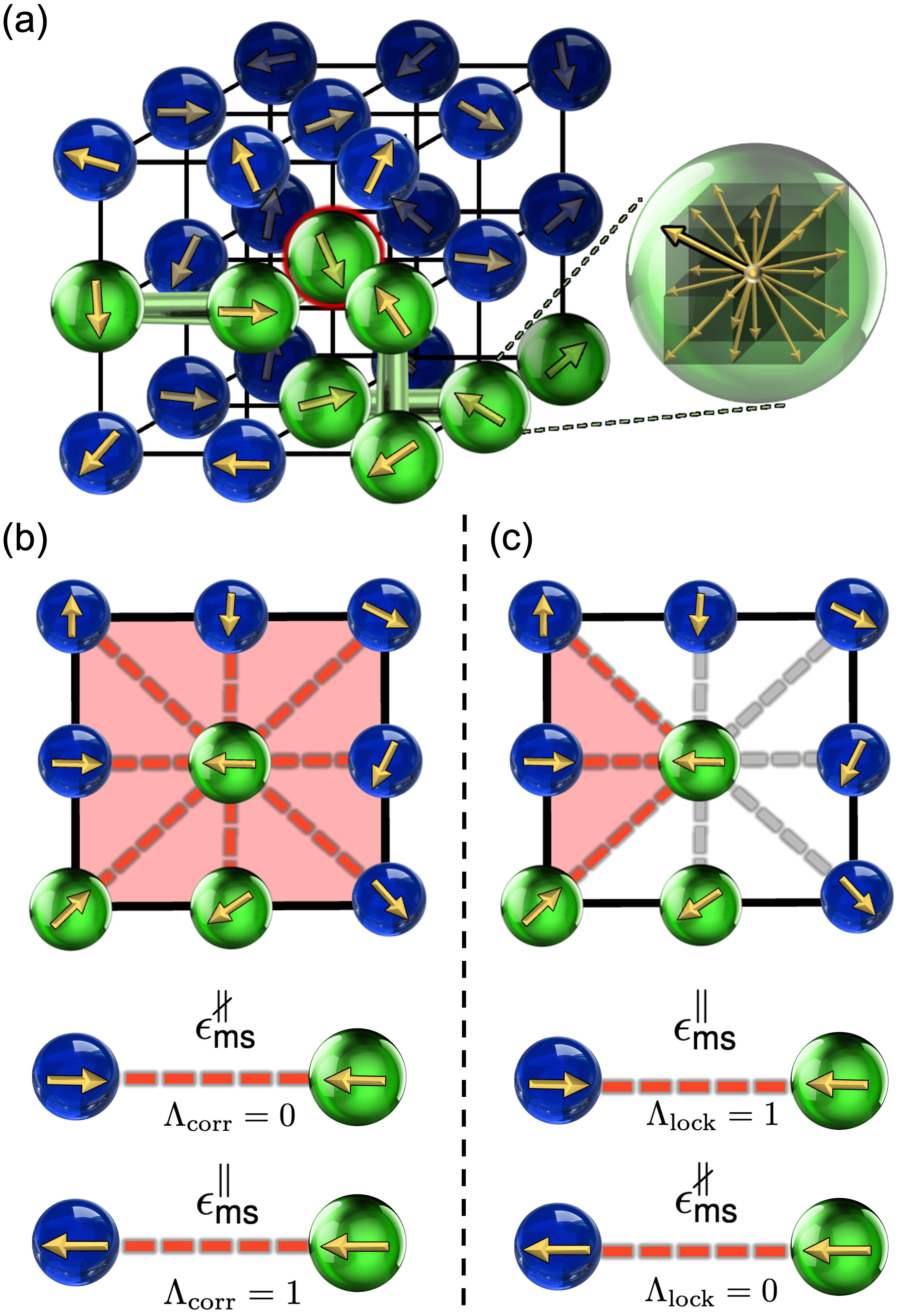
Figure 1: Schematic of the Flory-Huggins-Potts framework for a simple cubic lattice. (a) Depiction of the local neighborhood of a site (red outline). There are $z=26$ neighbors from nearest, next-nearest, and next-next-nearest lattice sites; particle orientations (arrows) discretely direct towards any of these neighbors. Monomer (m) segments are represented as green beads, solvent (s) particles as blue, and bonds as green cylinders, which can be across lattice edges, diagonals, or body diagonals. (b, c) Two-dimensional illustrations of (b) correlation network versus (c) locking interactions. In both panels, particles adjoined by red arrows can engage in aligned ($\parallel$) interactions, while those adjoined by gray only exhibit misaligned ($\nparallel$) interactions; the shaded red region highlights the fraction of neighbors that can engage in aligned interactions $p_{v}$. For (b), $p_{v}=1$ according to Eq. (4), whereas for (c), $p_{v}=3/8$ based on the restriction imposed by Eq. (5).

We consider a lattice with each site occupied by either a solvent particle or a monomer segment (Fig. 1a). Like FH, short-ranged, pairwise interactions exist between particles, and polymers consist of bonded monomer segments, and like a $q$-state Potts model, particles possess orientations that can influence pairwise energies. The system energy follows as

$$\mathcal{H} =\frac{1}{2}\sum_{i=1}^{N}\sum_{j\in\mathcal{N}(i)}\varepsilon\left(\alpha_{i},\alpha_{j},\hat{\sigma}_{i},\hat{\sigma}_{j}\right)+\sum_{k=1}^{m}\sum_{l=1}^{M-1}V\left(\vec{r}_{l+1}^{(k)},\vec{r}_{l}^{(k)}\right)$$ (1)

with

$$V\left(\vec{r}_{l+1}^{(k)},\vec{r}_{l}^{(k)}\right)=\begin{cases}0&\text{if }\left|\vec{r}_{l+1}^{(k)}-\vec{r}_{l}^{(k)}\right|\in\mathcal{N}(\mathcal{O})\\ \infty&\text{otherwise}\end{cases}$$ (2)

where $\alpha_{i}$ denotes the species (monomer or solvent) and $\hat{\sigma}_{i}$ denotes the unit-vector orientation of the the particle occupying the $i$th lattice site; $\varepsilon(\cdot)$ is a pairwise energy function of such variables; $N$ is the total number of lattice sites; $m$ is the number of polymer chains; $M$ is the number of monomer segments per chain; $\vec{r}_{l}^{(k)}$ is the position of the $l$th monomer segment in the $k$th polymer chain; and $V(\cdot)$ is a potential function that ensures bonded monomer segments occupy neighboring positions on the lattice (their distance is in the neighborhood of the origin, $\mathcal{N}(\mathcal{O})$). Eq. (1) is distinguished from FH by the influence of particle orientations on pairwise energies.

We propose that interaction asymmetries, which may arise from detailed chemical structure and molecular geometry, can be captured at coarse-grained resolution via lattice-site orientations. To simplify, we decompose

$$\varepsilon(\alpha_{i},\alpha_{j},\hat{\sigma}_{i},\hat{\sigma}_{j})=\epsilon_{\alpha_{i}\alpha_{j}}^{\nparallel}+\Lambda(i,j)\Delta_{\alpha_{i}\alpha_{j}}$$ (3)

where $\Delta_{\alpha_{i}\alpha_{j}}=\epsilon_{\alpha_{i}\alpha_{j}}^{\parallel}-\epsilon_{\alpha_{i}\alpha_{j}}^{\nparallel}$ is the difference between interaction energies for $\alpha_{i}$ and $\alpha_{j}$ species in an “aligned” ($\parallel$) versus “misaligned” ($\nparallel$) state, and $\Lambda(i,j)\in[0,1]$ functionally determines the extent to which particles at lattice sites $i$ and $j$ are aligned. By convention, we presume $\Delta_{\alpha_{i}\alpha_{j}}\leq 0$, such that aligned interactions are more energetically favorable than misaligned.

We suggest two physically motivated manifestations of $\Lambda$, colloquially referenced as correlation networks (Fig. 1b) and locking interactions (Fig. 1c) for our study. Inspired by hydrogen-bonding networks,[60] correlation-networks use

$$\Lambda_{\text{corr}}(i,j)=\Theta(\hat{\sigma}_{i}\cdot\hat{\sigma}_{j}-\delta),$$ (4)

and inspired by specific associative interactions[61, 62, 63] (e.g., hydrogen-bonding, metal–ligand, electrostatic), locking interactions use

$$\Lambda_{\text{lock}}(i,j)=\Theta(\delta-\left[\arccos\left(\hat{r}_{ji}\cdot\hat{\sigma}_{i}\right)+\arccos\left(\hat{r}_{ij}\cdot\hat{\sigma}_{j}\right)\right])$$ (5)

where $\hat{r}_{ij}=\frac{\vec{r}_{i}-\vec{r}_{j}}{|\vec{r}_{i}-\vec{r}_{j}|}$. In both Eqs. (4) and (5), $\Theta(\cdot)$ denotes a Heaviside step function such that $\delta$ effectively controls when particle orientations are aligned. A primary distinction between $\Lambda_{\text{corr}}$ and $\Lambda_{\text{lock}}$ is the fraction of neighboring particles capable of engaging in aligned interactions, denoted $p_{v}$. For $\Lambda_{\text{corr}}$, aligned interactions occur when particle orientations have the same direction (within the specified threshold $\delta$), allowing all neighboring particles to participate without restrictions. Conversely, for $\Lambda_{\text{lock}}$, aligned interactions require particle orientations to be directed towards the other particle, limiting possible aligned interactions to only a subset of neighboring particles. Therefore, $p_{v}=1$ for $\Lambda_{\text{corr}}$, while $p_{v}\leq 1$ for $\Lambda_{\text{lock}}$ (see Figs. 1b,c). There are many reasonable choices for expressing interaction anisotropy, and FHP is not exclusive to Eqs. (4) and (5).

To first gain insight into how thermoresponsiveness might manifest within the FHP framework, we utilize mean-field analysis of Eq. (1) to characterize phase behavior. Following general principles of FH and Boltzmann statistics (Supplemental Material, Section S1), the free energy of mixing per particle follows as

$$\frac{\Delta\bar{F}_{\text{mix}}}{k_{\text{B}}T}=\chi_{\text{FHP}}(T)\,\varphi(1-\varphi)\\ +\frac{\varphi}{M}\ln\varphi+(1-\varphi)\ln(1-\varphi)$$ (6)

where $\varphi$ is the volume fraction of the polymer and

$$\chi_{\text{FHP}}(T)\equiv\chi_{\text{FH}}(T)+\tilde{\chi}(T)$$ (7)

with

$$\chi_{\text{FH}}(T)\equiv\frac{(z-2)}{k_{\text{B}}T}\left(\epsilon_{\text{ms}}^{\nparallel}-\frac{1}{2}\left(\epsilon_{\text{mm}}^{\nparallel}+\epsilon_{\text{ss}}^{\nparallel}\right)\right)$$ (8)

being equivalent to a FH interaction parameter for a lattice with coordination number $z$ and pairwise energies set at the misaligned energy scale. Furthermore, the perturbation term

$$\tilde{\chi}(T)\equiv\frac{(z-2)}{k_{\text{B}}T}p_{v}\left(\tilde{\Delta}_{\text{ms}}(T)-\frac{1}{2}\left(\tilde{\Delta}_{\text{mm}}(T)+\tilde{\Delta}_{\text{ss}}(T)\right)\right)$$ (9)

accounts for asymmetry between aligned and misaligned interactions and their relative prevalence. In particular, the $\tilde{\Delta}_{ij}$ terms amount to per-site free-energy corrections between aligned and misaligned states given by

$$\tilde{\Delta}_{ij}(T)=\frac{\Delta_{ij}}{1+r\exp(\Delta_{ij}/k_{\text{B}}T)}$$ (10)

where $r=\frac{1-p_{\Omega}}{p_{\Omega}}$ is the fraction of possible misaligned microstates relative to aligned microstates for a given pair of particles. With Eqs. (6)-(10), the phase behavior for any given set of parameters can be characterized using the spinodal condition $(\partial^{2}\Delta\bar{F}_{\text{mix}}/\partial\varphi^{2})_{T}=0$ to identify stability limits of single, homogeneous phases.

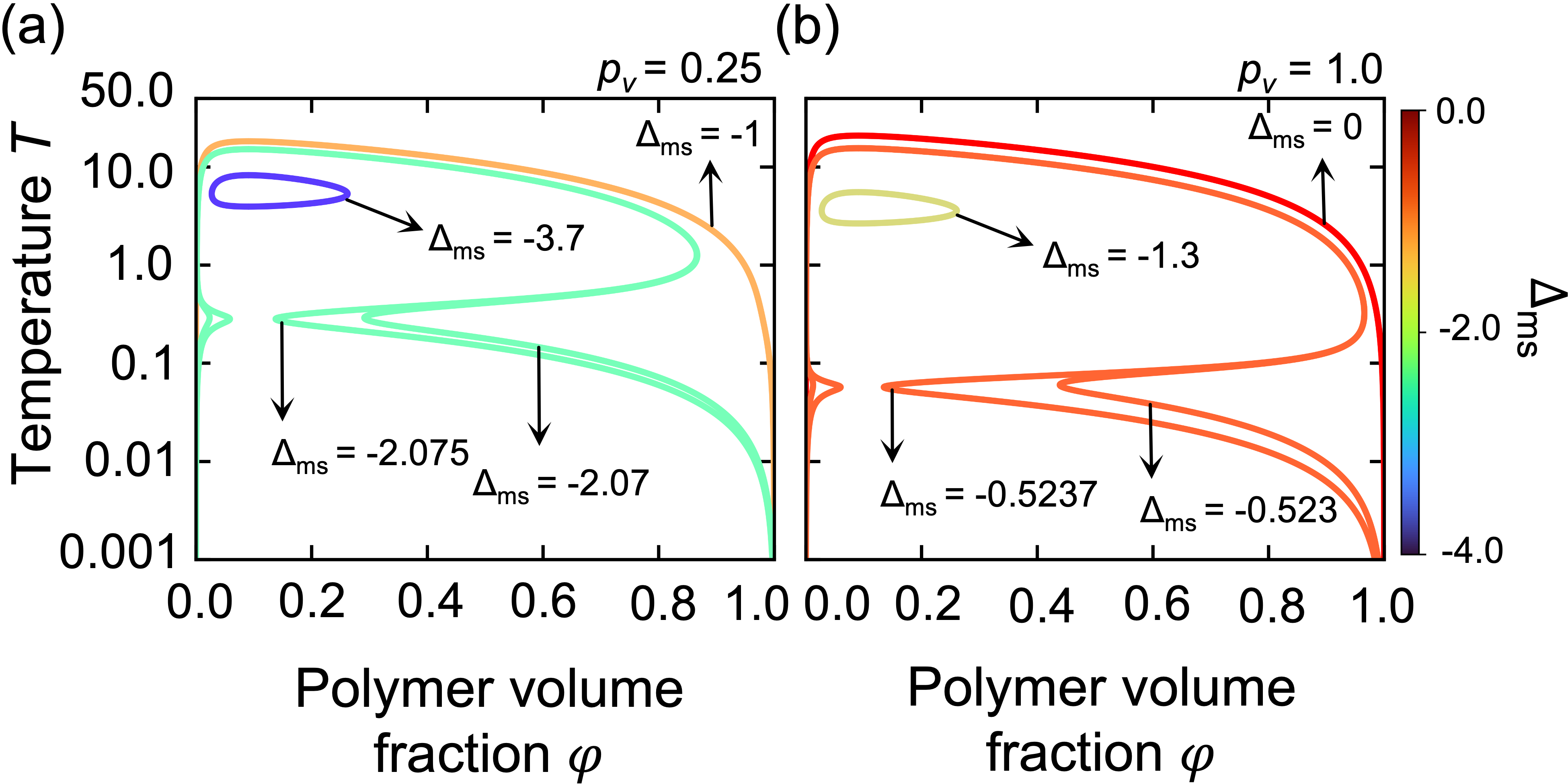
Figure 2: Representative temperature-volume fraction ($T-\varphi$) phase behavior of polymer solutions described by the Flory-Huggins-Potts framework. (a,b) Spinodal curves obtained from mean-field analysis for various $\Delta_{\text{ms}}=\epsilon^{\parallel}_{\text{ms}}-\epsilon^{\nparallel}_{\text{ms}}$ for (a) locking interactions with $p_{v}=0.25$ and (b) correlation network interactions. In both panels, parameters other than $\epsilon_{\text{ms}}^{\parallel}$ are fixed as $(\epsilon_{\text{mm}}^{\parallel},\epsilon_{\text{mm}}^{\nparallel},\epsilon_{\text{ms}}^{\nparallel},\epsilon_{\text{ss}}^{\parallel},\epsilon_{\text{ss}}^{\nparallel},p_{\Omega})$ = (-1,-1,0,0,0, 0.25).

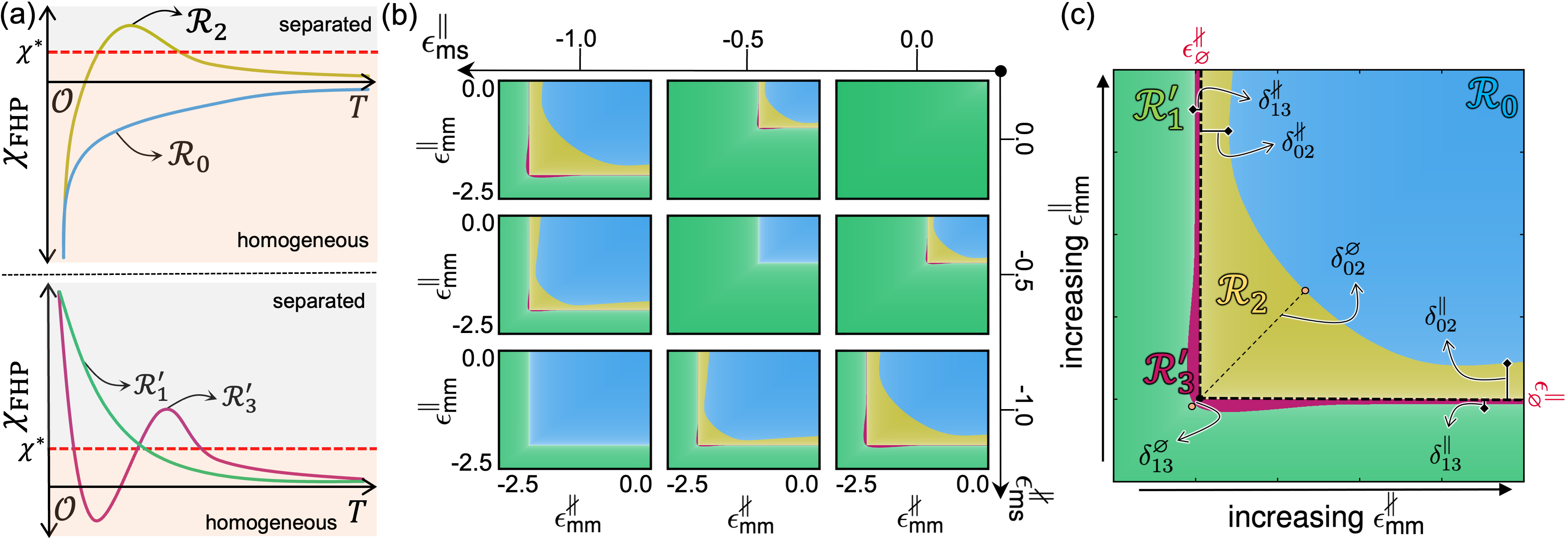
Figure 3: Characterization of phase behavior in FHP across different energetic regimes. (a) Qualitative examples of $\chi_{\text{FHP}}(T)\,$for classification of phase behavior. Systems characterized as $\mathcal{R}_{0}\,$are expected to always be homogeneous, while those from $\mathcal{R}_{1}^{\prime}\,$, $\mathcal{R}_{2}\,$, and $\mathcal{R}_{3}^{\prime}\,$ respectively feature upper critical solution temperatures, miscibility loops, and hourglass-shaped phase envelopes. (b) Hyperphase diagram illustrating classification of phase behavior as a function of $\epsilon_{\text{mm}}^{\parallel}$ and $\epsilon_{\text{mm}}^{\nparallel}$ (inner plots) at various values of $\epsilon_{\text{ms}}^{\parallel}$ and $\epsilon_{\text{ms}}^{\nparallel}$ (outer axes). Results are obtained from mean-field analysis with $(\epsilon_{\text{ss}}^{\parallel},\epsilon_{\text{ss}}^{\nparallel},p_{v},p_{\Omega})$ =(0, 0, 1, 0.25) and $z=26$. Additional results are shown in Fig. S1 of the Supplemental Materials. (c) Qualitative decomposition of phase behavior deduced from the determination of eight reference elements: $\epsilon^{\parallel}_{\varnothing}$, $\epsilon^{\nparallel}_{\varnothing}$, $\delta_{02}^{\parallel}$, $\delta_{02}^{\nparallel}$, $\delta_{13}^{\parallel}$, $\delta_{13}^{\nparallel}$, $\delta_{02}^{\varnothing}$, and $\delta_{13}^{\varnothing}$. The reference elements are summarized in Eqs. (11)-(13) with full derivation and discussion in Supplemental Materials, Section S4.

Fig. 2 illustrates how the FHP framework exhibits complex phase behavior relative to FH when monomer-solvent interactions are anisotropic (i.e., $\Delta_{\text{ms}}\leq\Delta_{\text{mm}}=\Delta_{\text{ss}}=0$). Decreasing $\Delta_{\text{ms}}$ (favoring aligned monomer-solvent interactions) progresses spinodal curves from UCST to hourglass-like phase envelopes and later to miscibility loops. The presence of hourglasses and miscibility loops indicate transitions from homogeneous to phase-separated states upon heating at particular compositions – a phenomenon absent in standard FH; this occurs for correlation-network and locking interactions, with the former progressing at lesser $\Delta_{\text{ms}}$.

The complex phase behavior native to FHP derives from non-trivial temperature-dependence of $\chi_{\text{FHP}}(T)\,$. Phase-separated states are predicted to occur if $\chi_{\text{FHP}}(T)\,$exceeds a critical value of $\chi^{*}$, which satisfies $(\partial^{2}\Delta\overline{F}_{\text{mix}}/\partial^{2}\varphi)_{T}=0$ and $(\partial^{3}\Delta\overline{F}_{\text{mix}}/\partial^{3}\varphi)_{T}=0$. For $M=32$, the spinodal region spans conditions for which $\chi_{\text{FHP}}(T)\,\geq\chi^{*}\approx 0.692$ (Supplemental Material, Section S2). In FH, $\chi_{\text{FH}}(T)$ is monotonic and either strictly positive or strictly negative, depending on the pairwise interaction parameters ($\epsilon_{\text{mm}},\epsilon_{\text{ss}},\epsilon_{\text{ms}}$); this implies that UCST will only be observed if $\lim_{T\to 0}\chi_{\text{FH}}(T)>\chi^{*}$. In FHP, based on the results of Fig. 2, we anticipate four qualitatively distinct behaviors for $\chi_{\text{FHP}}(T)\,$, denoted as $\mathcal{R}_{0}\,$, $\mathcal{R}_{1}^{\prime}\,$, $\mathcal{R}_{2}\,$, or $\mathcal{R}_{3}^{\prime}\,$ (Fig. 3a). The notation is such that the subscript indicates the number of homogeneous-to-phase-separated transitions, a prime (^′) indicates a phase-separated state at low $T$, and no prime indicates a homogeneous state at low $T$. Mathematically, $\mathcal{R}_{0}\,$ relates to $\chi_{\text{FHP}}(T)\,<\chi^{*}$, yielding only homogeneous phases; $\mathcal{R}_{1}^{\prime}\,$ is initially phase-separated ($\chi_{\text{FHP}}(T)\,>\chi^{*}$) at low $T$ then tends to zero, implying UCST; $\mathcal{R}_{2}\,$ is $\chi_{\text{FHP}}(T)\,<\chi^{*}$ at low $T$, transitions to $\chi_{\text{FHP}}(T)\,>\chi^{*}$, then tends to zero, implying a miscibility loop; and $\mathcal{R}_{3}^{\prime}\,$ is $\chi_{\text{FHP}}(T)\,>\chi^{*}$ at low $T$ with transitions below and above $\chi^{*}$ before tending to zero, implying hour-glass behavior.

With this conceptual scaffolding, we examine how pairwise parameters dictate $\mathcal{R}_{0}\,$, $\mathcal{R}_{1}^{\prime}\,$, $\mathcal{R}_{2}\,$, or $\mathcal{R}_{3}^{\prime}\,$. Fig. 3b provides a “hyperphase diagram” summarizing $\chi_{\text{FHP}}(T)\,$ behavior as a function of $\epsilon_{\text{ms}}^{\parallel}$, $\epsilon_{\text{ms}}^{\nparallel}$, $\epsilon_{\text{mm}}^{\parallel}$, and $\epsilon_{\text{mm}}^{\nparallel}$ (other parameters fixed). While the preponderance of parameter-space yields $\mathcal{R}_{0}\,$ (blue) or $\mathcal{R}_{1}^{\prime}\,$ (green) behavior, depending on whether monomer-solvent or monomer-monomer interactions, respectively, dominate at low $T$, $\mathcal{R}_{2}\,$ (miscibility loops, yellow) and $\mathcal{R}_{3}^{\prime}\,$ (hourglass envelopes, magenta) emerge within intermediate energetic regimes. Strikingly, we confirm over a broader set of parameters that asymmetry in monomer-solvent interactions is essential to observe these phenomena. By consequence, behavior defined by both $\mathcal{R}_{2}\,$ and $\mathcal{R}_{3}^{\prime}\,$ comprise a greater fraction of parameter-space when there are greater disparities between aligned versus misaligned monomer-solvent interactions. Nevertheless, $\mathcal{R}_{3}^{\prime}\,$ only appears in a narrow energetic regime bordering $\mathcal{R}_{1}^{\prime}\,$and $\mathcal{R}_{2}\,$, indicating that an intricate balance of interactions is necessary to produce multiple inflection points in $\chi_{\text{FHP}}(T)\,$ in the vicinity of $\chi^{*}$. These general observations hold for other parameter sets (Supplemental Material, Section S3 and Fig. S1). Overall, the diagram illustrates how both homotypic and heterotypic interactions as well as misaligned and aligned interactions balance to give rise to nuanced phase behavior.

The phase behavior captured by FHP can be parametrically delineated by analyzing the mean-field equations. Here, we discuss the approach and key results for $p_{v}=1$ and $\epsilon_{\text{ss}}^{\parallel}=\epsilon_{\text{ss}}^{\nparallel}=0$, leaving more general discussion to Section S4 of the Supplemental Materials. For a given a set of monomer-solvent interactions, we identify eight reference elements (see Fig. 3c) that chart out how parameter-space roughly divides by phase behavior. These reference elements are summarized as

$$\epsilon_{\varnothing}\equiv\epsilon^{\parallel}_{\varnothing}=\epsilon^{\nparallel}_{\varnothing}=2\min\left(\epsilon^{\parallel}_{\text{ms}},\epsilon^{\nparallel}_{\text{ms}}\right),$$ (11)

$$\delta_{\mu\nu}^{\infty}\equiv\delta^{\parallel}_{\mu\nu}=\delta^{\nparallel}_{\mu\nu}=2\tilde{\Delta}_{\text{ms}}(T_{\mu\nu}^{*})-\frac{2k_{\text{B}}T_{\mu\nu}^{*}}{z-2}\chi^{*},$$ (12)

and

$$\delta^{\varnothing}_{\mu\nu}=\sqrt{2}\left(\delta_{\mu\nu}^{\infty}+2\epsilon_{\text{ms}}^{\nparallel}-\epsilon_{\varnothing}\right).$$ (13)

In effect, $\epsilon_{\varnothing}$ denotes the strength of monomer-monomer interactions required to balance monomer-solvent interactions, thereby distinguishing homogeneous versus phase-separated states at low-temperatures. Meanwhile, the “widths” $\delta_{\mu\nu}^{\infty}$ and $\delta^{\varnothing}_{\mu\nu}$, for which $(\mu,\nu)$ = (0,2) or (1,3), indicate the extent of parameter-space yielding $\mathcal{R}_{2}\,$ rather than $\mathcal{R}_{0}\,$ or $\mathcal{R}_{3}^{\prime}\,$ rather than $\mathcal{R}_{1}^{\prime}\,$ at different points of the dividing boundaries; the temperatures $T_{02}^{*}$ and $T_{13}^{*}$ coincide with $\chi_{\text{FHP}}(T)\,$ = $\chi^{*}$ as described later.

Eqs. (11)-(13) are obtained by considering how $\chi_{\text{FHP}}(T)\,$ can remain strictly homogeneous ($\mathcal{R}_{0}\,$) or simply exhibit UCST ($\mathcal{R}_{1}^{\prime}\,$). For Eq. (11), we recognize that both $\mathcal{R}_{0}$ and $\mathcal{R}_{2}$ imply a homogeneous system at low $T$ ($\lim_{T\rightarrow 0^{+}}\chi_{\text{FHP}}(T)\,\rightarrow-\infty$) while $\mathcal{R}_{1}^{\prime}$ and $\mathcal{R}_{3}^{\prime}$ imply a phase-separated system ($\lim_{T\rightarrow 0^{+}}\chi_{\text{FHP}}(T)\,\rightarrow\infty$). Therefore, the transition must coincide with $\lim_{T\rightarrow 0^{+}}\chi_{\text{FHP}}(T)\,=0$. When $p_{v}=1$, this results in an $L$-shaped boundary where monomer-monomer interactions are given by $\epsilon_{\varnothing}$. For the widths of $\mathcal{R}_{2}\,$ expressed by Eq. (12) (i.e., $\delta_{02}^{\infty}$), we note that $\mathcal{R}_{0}$ and $\mathcal{R}_{2}$ have the same limiting behavior at low and high $T$. Consequently, the boundary between must be such that $\chi_{\text{FHP}}(T)\,$ never exceeds $\chi^{*}$, which implies $\max\chi_{\text{FHP}}(T)\,=\chi^{*}$ at some parameter-set-dependent temperature $T_{02}^{*}$. Using these conditions to solve for $\epsilon_{\text{mm}}^{\parallel}$ as $\epsilon_{\text{mm}}^{\nparallel}\to\infty$ and for $\epsilon_{\text{mm}}^{\nparallel}$ as $\epsilon_{\text{mm}}^{\parallel}\to\infty$ yields $\delta_{02}^{\infty}$. Similar arguments yield $\delta_{13}^{\infty}$; in this case, however, $\chi_{\text{FHP}}(T)\,$ must initially exceed $\chi^{*}$ over a single, continuous temperature interval. For Eq. (13), we enforce the same constraints as Eq. (12) but instead consider isotropic monomer-monomer interactions ($\Delta_{\text{mm}}\to 0$). Notably, whereas Eq. (11) also applies to FH, Eqs. (12) and (13) critically depend on $\Delta_{\text{ms}}$, which is unique to the parameteric landscape of FHP. In aggregate, this analysis transparently connects the complex phase behavior of FHP with its essential parameters.

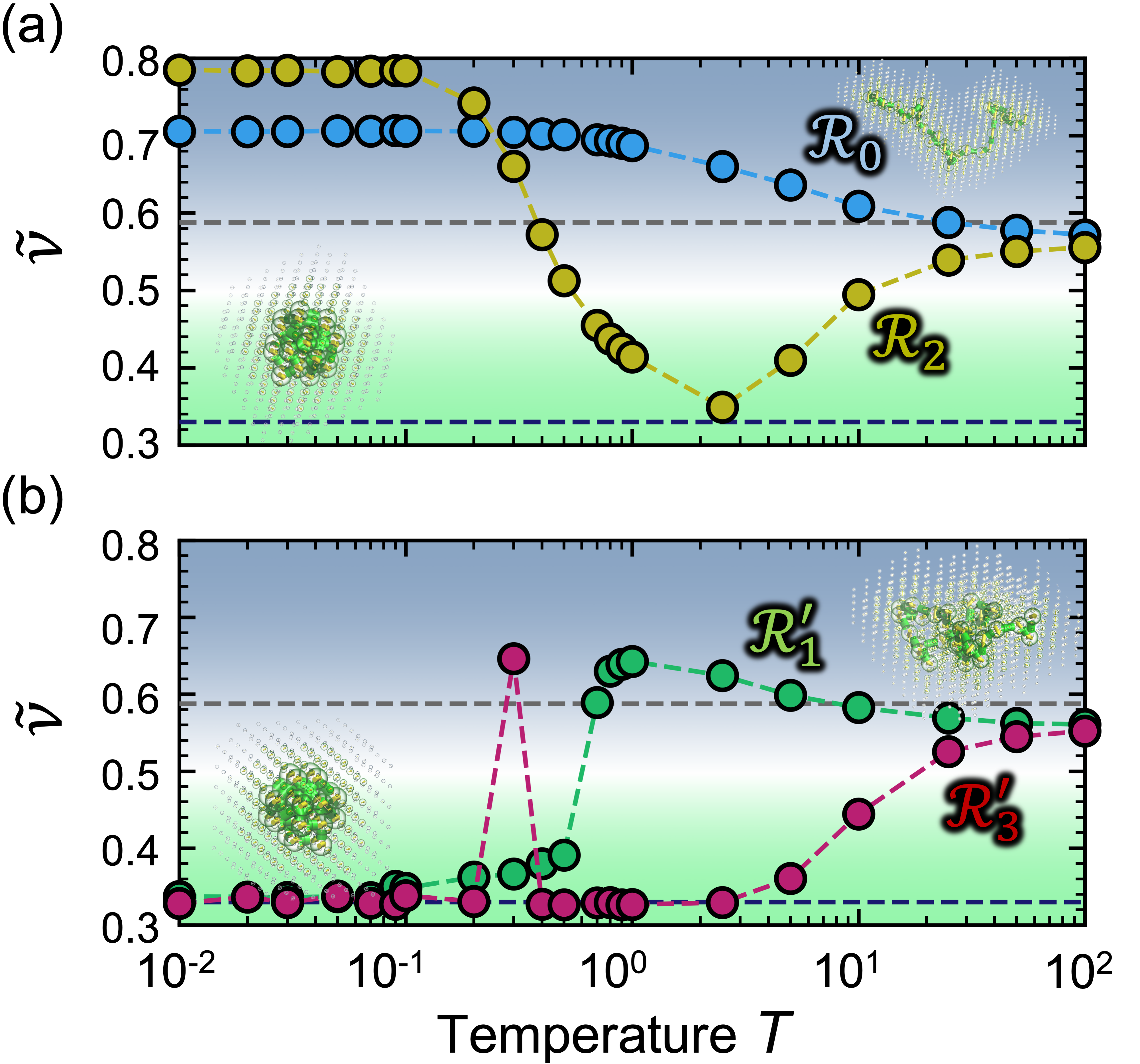
Figure 4: Temperature-dependent conformational behavior of single polymer chains in different energetic regimes. (a, b) Intra-chain scaling exponent $\tilde{\nu}$ obtained from Monte Carlo simulations of single polymer chains using parameters sets associated with (a) $\mathcal{R}_{0}\,$ and $\mathcal{R}_{2}\,$ and (b) $\mathcal{R}_{1}^{\prime}\,$ and $\mathcal{R}_{3}^{\prime}\,$. Data specifically generated using $(\epsilon_{\text{mm}}^{\parallel},\epsilon_{\text{mm}}^{\nparallel},\epsilon_{\text{ms}}^{\parallel},\epsilon_{\text{ms}}^{\nparallel})$ = (-1,-1,-1,-1) for $\mathcal{R}_{0}\,$, (-2.2, -1, -1, -1) for $\mathcal{R}_{1}^{\prime}\,$, (-1.5,-1.5,-1,0) for $\mathcal{R}_{2}\,$, and (-2.001, -2.001, -1, 0) for $\mathcal{R}_{3}^{\prime}\,$. All simulations utilize correlation-network interactions with $\delta$ such that $p_{\Omega}$ = 0.25 and also set $\epsilon_{\text{ss}}^{\parallel}$ = $\epsilon_{\text{ss}}^{\nparallel}$ = 0. Error bars are smaller than the symbol size. The horizontal dashed lines are guides to the eye for globular scaling (black) and excluded-volume statistics (gray). The background color gradient is based on values of $\tilde{\nu}$ to emphasize conformations that are more expanded (blue) or more globular (green) relative to the ideal chain (white).

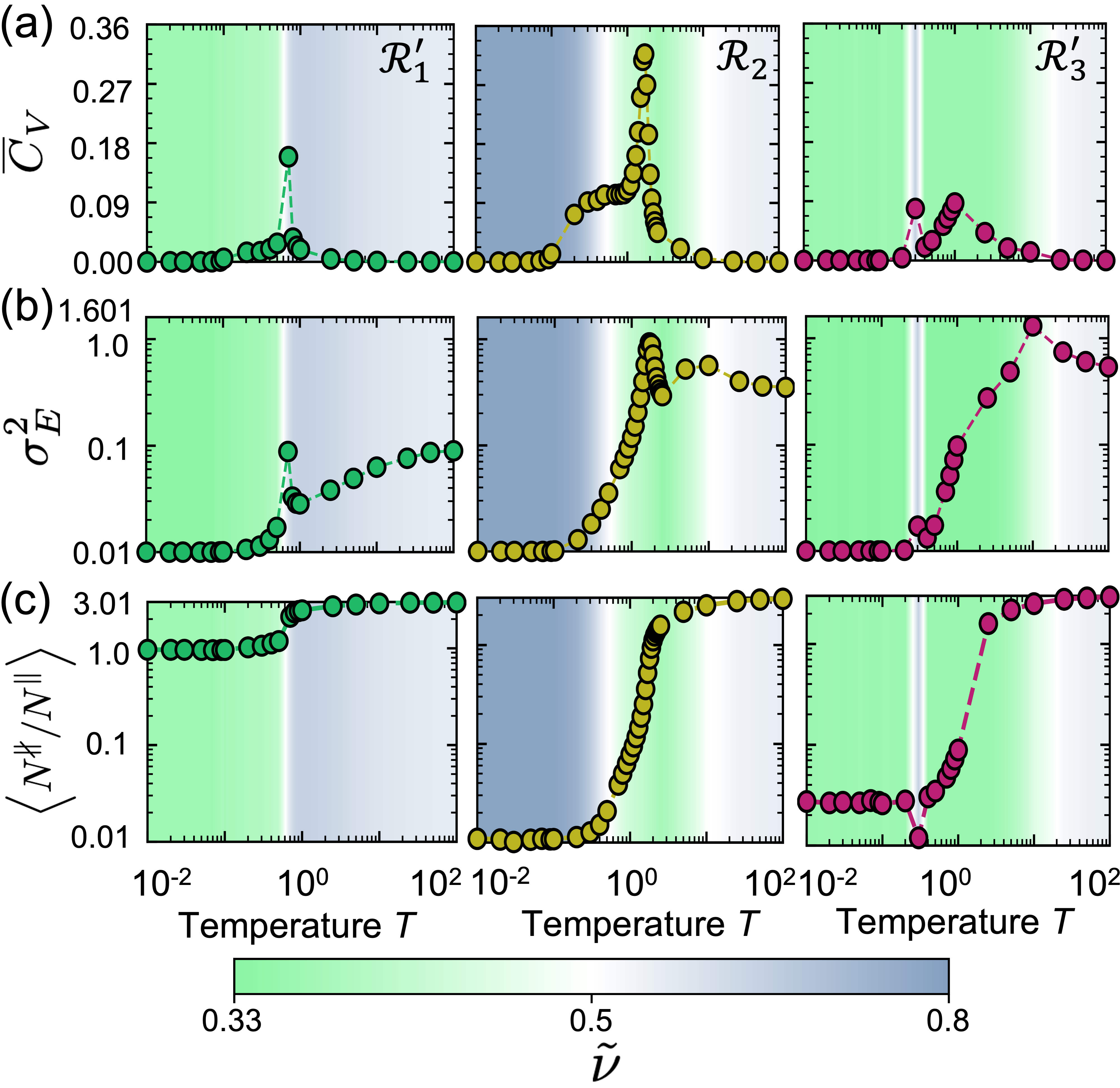
Figure 5: Examination of microscopic signatures of conformational transitions observed in different energetic regimes. Quantities include (a) heat capacity $\overline{C}_{V}$, (b) fluctuations in total energy $\sigma_{E}^{2}$, and (c) the average proportion of misaligned to aligned interactions $N^{\nparallel}/N^{\parallel}$. Plots in panels (b) and (c) have been shifted by $0.01$ to highlight the variation in the quantity as the conformation of the polymer changes. Each panel displays data obtained from Monte Carlo simulation of single polymer chains using parameters sets associated with $\mathcal{R}_{1}^{\prime}\,$, $\mathcal{R}_{2}\,$, and $\mathcal{R}_{3}^{\prime}\,$, arranged left-to-right. Results are reported for the same simulations in Fig. 4, such that the background color reflects the value $\tilde{\nu}$ at the given temperature based on interpolation.

The physics dictating phase behavior are also often presumed to govern microscopic phenomena, such as coil-globule transitions,[15, 17, 64] and consistency has been established between single chain structure and solution thermodynamics for FH.[49, 65] To ascertain whether such a connection exists for the FHP framework, we characterize the temperature-dependent behavior of single polymer chains using Metropolis Monte Carlo (MC) simulation with Eqs. (1)-(5). All simulations feature a $34\times 34\times 34$ simple cubic lattice with periodic boundaries; lattice sites are occupied by solvent particles and a single polymer chain with $M=32$. We use $z=26$ (accounting for interactions between nearest, next-nearest, and next-next-nearest neighboring sites) and restrict particle orientations to direct towards the 26 neighboring sites (Fig. 1a). MC moves for solvent particles include solvent-orientation exchanges and group-level orientation perturbations. MC moves for the polymer include conventional end-rotation, reptation, orientation perturbations, and chain regrowth with orientation perturbations. To enhance sampling efficiency, chain-regrowth moves are implemented using a Rosenbluth sampling scheme.[66] All simulations consist of $10^{8}$ MC moves with the latter half used for analysis; averages are obtained from 30 independent trajectories with all errors representing the standard error of the mean. Additional details can be found in Supplemental Materials, Section S5.

Single-chain conformational statistics exhibit clear signatures of phase behavior from the FHP framework. To illustrate, we perform simulations using parameters from each of $\mathcal{R}_{0}\,$, $\mathcal{R}_{1}^{\prime}\,$, $\mathcal{R}_{2}\,$, and $\mathcal{R}_{3}^{\prime}\,$, at several temperatures, to extract intra-chain scaling exponents $\tilde{\nu}$ defined by

$$\left\langle|\vec{r}_{i}-\vec{r}_{j}|^{2}\right\rangle\propto|i-j|^{2\tilde{\nu}};$$ (14)

this allows approximate comparison with known scaling laws (e.g., $R_{\text{g}}\propto M^{1/2}$ for ideal chains, $R_{\text{g}}\propto M^{1/3}$ for globules); the results are in Fig. 4. At low $T$, systems characterized by parameters from $\mathcal{R}_{0}\,$ and $\mathcal{R}_{2}\,$ exhibit scaling indicative of good-solvent conditions ($\tilde{\nu}\geq 2/3$), while systems from $\mathcal{R}_{1}^{\prime}\,$ and $\mathcal{R}_{3}^{\prime}\,$ display more globular scaling (Fig. 4b); this correlates with $\mathcal{R}_{0}\,$ and $\mathcal{R}_{2}\,$ having a single homogeneous phase and $\mathcal{R}_{1}^{\prime}\,$ and $\mathcal{R}_{3}^{\prime}\,$ featuring phase-separated states. Behavior between $\mathcal{R}_{0}\,$ and $\mathcal{R}_{2}\,$ differs upon heating. While $\tilde{\nu}$ from $\mathcal{R}_{0}\,$ gradually approaches excluded-volume statistics ($\tilde{\nu}\sim 0.588$), $\tilde{\nu}$ from $\mathcal{R}_{2}\,$ collapses to a globule before expanding in the high-$T$ limit. This coil-globule transition, followed by expansion, aligns with a miscibility loop, indicating homogeneous then phase-separated then homogeneous states upon heating. Similar explanations apply for $\mathcal{R}_{1}^{\prime}\,$ and $\mathcal{R}_{3}^{\prime}\,$. The singular globule-coil transition for $\tilde{\nu}$ from $\mathcal{R}_{1}^{\prime}\,$ is consistent with an UCST, while $\tilde{\nu}$ from $\mathcal{R}_{3}^{\prime}\,$ begins as globular then crosses the ideal-chain limit three times–a progression consistent with an hourglass-like phase envelope. Notably, $\tilde{\nu}$ obtained with FH (Supplemental Materials, Fig. S3) only tends gradually and monotonically to excluded-volume statistics upon heating. Thus, anisotropic interactions in FHP drive sharp, thermally induced conformational transitions reminiscent of trends in emergent phase behavior.

We also identify key molecular-level signatures associated with the observed conformational transitions. We specifically monitor the heat capacity $\overline{C}_{V}$ (Fig. 5a), energy fluctuations $\sigma^{2}_{E}$ (Fig. 5b), and relative proportion of misaligned to aligned interactions $N^{\nparallel}/N^{\parallel}$ (Fig. 5c); additional analysis relating relative energy contributions is in the Supplemental Materials (Figs. S4 and S5). For systems from $\mathcal{R}_{1}^{\prime}\,$, the single coil-globule transition is marked by maxima in $\overline{C}_{V}$ and $\sigma^{2}_{E}$ that coincide with increasing the proportion of misaligned interactions over narrow temperature range wherein $\tilde{\nu}\sim 0.5$ (white region). Similar observations hold for the low-$T$ transitions from a coil to a globule in $\mathcal{R}_{2}\,$ and $\mathcal{R}_{3}^{\prime}\,$, for which at least some enhancement in misaligned interactions accompanies peaks in $\overline{C}_{V}$. In addition, $\mathcal{R}_{2}\,$ and $\mathcal{R}_{3}^{\prime}\,$ display a second higher-$T$ transition from globular to excluded-volume statistics that is only captured by a maximum in $\sigma^{2}_{E}$ as $N^{\nparallel}/N^{\parallel}$ plateaus towards a limiting high-$T$ value of $r=(1-p_{\Omega})/p_{\Omega}$. With the current data, however, we do not find perfect alignment with critical temperatures and these markers for single-chain transitions (Supplemental Materials, Section S10). Nevertheless, sharp peaks in $\overline{C}_{V}$ and/or $\sigma^{2}_{E}$ provide reasonable markers for single-chain conformational transitions, which are ultimately driven by compositional and orientational changes in the polymer’s local environment (Fig. S5).

In conclusion, we have introduced the Flory-Huggins-Potts (FHP) framework to describe and understand thermoresponsive polymer solutions. Remarkably, this approach, which simply extends Flory-Huggins (FH) theory with orientation-dependent interactions, showcases diverse temperature-dependent phase behavior, including miscibility loops and hourglass-like phase envelopes unseen in simple FH models. Importantly, this phase behavior emerges without any ad hoc functional dependencies on temperature; the effects are transparently attributable to disparities in pairwise interaction energies introduced by the orientational degrees of freedom. Consequently, we can fully map the phase behavior across all parametric regimes using mean-field analysis. Specifically considering dependence on $\epsilon_{\text{mm}}^{\parallel}$, $\epsilon_{\text{mm}}^{\nparallel}$, $\epsilon_{\text{ms}}^{\parallel}$, and $\epsilon_{\text{ms}}^{\nparallel}$ revealed that disparity between $\epsilon_{\text{ms}}^{\parallel}$ and $\epsilon_{\text{ms}}^{\nparallel}$ was critical to observe multiple phase transition temperatures. Importantly, because the FHP framework features only parameters related to particle interactions, we could straightforwardly investigate the underlying microscopic physics by means of Monte Carlo simulation. We find strong correspondence between single-chain conformational behavior (obtained from numerical simulations) and macroscopic phase transitions (deduced from mean-field analysis), which aligns with conventional expectations of systems exhibiting heating-induced coil-globule transition also possessing lower-critical solution temperatures, for example. From this, we find that energetic fluctuations associated with enhancements in misaligned interactions likely underpin sharp thermal responses.

As a minimally complex framework, FHP can be extended beyond its application to understanding thermoresponsive polymer solutions in various ways. Firstly, it can serve as foundational scaffolding for exploring other stimuli-responsive behaviors grounded in similar physical principles. Secondly, the simplicity and transparency of FHP physics make it suitable for benchmarking and hypothesis testing. A promising avenue lies in developing robust bottom-up coarse-graining techniques for stimuli-responsive systems, addressing challenges related to the lack of underlying theory and sufficient ground-truth reference data. Future implementations could be leveraged to examine phenomena like hydrophobic collapse. Thirdly, there is potential for extending FHP to better align with true physical systems. While the present work emphasizes fundamental physics and a valuable conceptual framework, establishing connections with chemically realistic systems and achieving quantitative predictive power is crucial. Future efforts could involve deducing parameters for representing canonical thermoresponsive polymers, such as poly(N-isopropylacrylamide), and considering presently neglected factors like compressibility.

References

- Karimi et al. [2016] M. Karimi, P. S. Zangabad, A. Ghasemi, M. Amiri, M. Bahrami, H. Malekzad, H. G. Asl, Z. Mahdieh, M. Bozorgomid, A. Ghasemi, M. R. R. T. Boyuk, and M. R. Hamblin, ACS Applied Materials & Interfaces 8, 21107 (2016).
- Kim and Matsunaga [2017] Y.-J. Kim and Y. T. Matsunaga, Journal of Materials Chemistry B 5, 4307 (2017).
- Ward and Georgiou [2011] M. A. Ward and T. K. Georgiou, Polymers 3, 1215 (2011).
- Davis et al. [2009] D. A. Davis, A. Hamilton, J. Yang, L. D. Cremar, D. V. Gough, S. L. Potisek, M. T. Ong, P. V. Braun, T. J. Martínez, S. R. White, J. S. Moore, and N. R. Sottos, Nature 459, 68 (2009).
- Colson and Grinstaff [2012] Y. L. Colson and M. W. Grinstaff, Advanced Materials 24, 3878 (2012).
- Tanaka et al. [1982] T. Tanaka, I. Nishio, S.-T. Sun, and S. Ueno-Nishio, Science 218, 467 (1982).
- Thévenot et al. [2013] J. Thévenot, H. Oliveira, O. Sandre, and S. Lecommandoux, Chemical Society Reviews 42, 7099 (2013).
- Irie [1990] M. Irie, Pure and Applied Chemistry 62, 1495 (1990).
- Zhai [2013] L. Zhai, Chemical Society Reviews 42, 7148 (2013).
- Mukherji et al. [2019] D. Mukherji, M. D. Watson, S. Morsbach, M. Schmutz, M. Wagner, C. M. Marques, and K. Kremer, Macromolecules 52, 3471 (2019).
- Stuart et al. [2010] M. A. C. Stuart, W. T. S. Huck, J. Genzer, M. Müller, C. Ober, M. Stamm, G. B. Sukhorukov, I. Szleifer, V. V. Tsukruk, M. Urban, F. Winnik, S. Zauscher, I. Luzinov, and S. Minko, Nature Materials 9, 101 (2010).
- Mukherji et al. [2020] D. Mukherji, C. M. Marques, and K. Kremer, Annual Review of Condensed Matter Physics 11, 271 (2020).
- Xu et al. [2021] X. Xu, S. Ozden, N. Bizmark, C. B. Arnold, S. S. Datta, and R. D. Priestley, Advanced Materials 33, 2007833 (2021).
- Xu et al. [2022] X. Xu, N. Bizmark, K. S. S. Christie, S. S. Datta, Z. J. Ren, and R. D. Priestley, Macromolecules 55, 1894 (2022).
- Zeng et al. [2020] X. Zeng, A. S. Holehouse, A. Chilkoti, T. Mittag, and R. V. Pappu, Biophysical Journal 119, 402 (2020).
- Scarpa et al. [1967] J. S. Scarpa, D. D. Mueller, and I. M. Klotz, Journal of the American Chemical Society 89, 6024 (1967).
- Shakhnovich and Finkelstein [1989] E. I. Shakhnovich and A. V. Finkelstein, Biopolymers 28, 1667 (1989).
- de los Rios and Caldarelli [2000] P. de los Rios and G. Caldarelli, Physical Review E 62, 8449 (2000).
- Gelbart et al. [2000] W. M. Gelbart, R. F. Bruinsma, P. A. Pincus, and V. A. Parsegian, Physics Today 53, 38 (2000).
- Shin and Brangwynne [2017] Y. Shin and C. P. Brangwynne, Science 357 (2017), 10.1126/science.aaf4382.
- Dignon et al. [2019] G. L. Dignon, W. Zheng, Y. C. Kim, and J. Mittal, ACS Central Science 5, 821 (2019).
- Banani et al. [2017] S. F. Banani, H. O. Lee, A. A. Hyman, and M. K. Rosen, Nature Reviews Molecular Cell Biology 18, 285 (2017).
- Lyon et al. [2020] A. S. Lyon, W. B. Peeples, and M. K. Rosen, Nature Reviews Molecular Cell Biology 22, 215 (2020).
- Geary et al. [2014] C. Geary, P. W. K. Rothemund, and E. S. Andersen, Science 345, 799 (2014).
- Han et al. [2017] D. Han, X. Qi, C. Myhrvold, B. Wang, M. Dai, S. Jiang, M. Bates, Y. Liu, B. An, F. Zhang, H. Yan, and P. Yin, Science 358 (2017), 10.1126/science.aao2648.
- Jia et al. [2021] Y. Jia, L. Chen, J. Liu, W. Li, and H. Gu, Chem 7, 959 (2021).
- Flory [1949] P. J. Flory, The Journal of Chemical Physics 17, 303 (1949).
- Flory [1953] P. J. Flory, Principles of polymer chemistry (Ithaca, NY, Cornell University Press, 1953., 1953).
- de Gennes [1979] P. G. de Gennes, Scaling Concepts in Polymer Physics (Cornell University Press, 1979).
- Gennes [1975] P. D. Gennes, Journal de Physique Lettres 36, 55 (1975).
- Lacombe and Sanchez [1976] R. H. Lacombe and I. C. Sanchez, The Journal of Physical Chemistry 80, 2568 (1976).
- Sanchez and Lacombe [1976] I. C. Sanchez and R. H. Lacombe, The Journal of Physical Chemistry 80, 2352 (1976).
- Sanchez and Lacombe [1978] I. C. Sanchez and R. H. Lacombe, Macromolecules 11, 1145 (1978).
- Panayiotou [1987] C. G. Panayiotou, Macromolecules 20, 861 (1987).
- Panayiotou and Sanchez [1991] C. Panayiotou and I. C. Sanchez, The Journal of Physical Chemistry 95, 10090 (1991).
- Veytsman [1990] B. A. Veytsman, The Journal of Physical Chemistry 94, 8499 (1990).
- Simmons and Sanchez [2008] D. S. Simmons and I. C. Sanchez, Macromolecules 41, 5885 (2008).
- Simmons and Sanchez [2010] D. S. Simmons and I. C. Sanchez, Macromolecules 43, 1571 (2010).
- Dahanayake and Dormidontova [2021] R. Dahanayake and E. Dormidontova, Physical Review Letters 127, 167801 (2021).
- Matsuyama and Tanaka [1990] A. Matsuyama and F. Tanaka, Physical Review Letters 65, 341 (1990).
- Bekiranov et al. [1997] S. Bekiranov, R. Bruinsma, and P. Pincus, Physical Review E 55, 577 (1997).
- Choi et al. [2019] J.-M. Choi, F. Dar, and R. V. Pappu, PLOS Computational Biology 15, e1007028 (2019).
- Muller [1990] N. Muller, Accounts of Chemical Research 23, 23 (1990).
- Lee and Graziano [1996] B. Lee and G. Graziano, Journal of the American Chemical Society 118, 5163 (1996).
- Jeppesen and Kremer [1996] C. Jeppesen and K. Kremer, Europhysics Letters (EPL) 34, 563 (1996).
- Martin et al. [2020] E. W. Martin, A. S. Holehouse, I. Peran, M. Farag, J. J. Incicco, A. Bremer, C. R. Grace, A. Soranno, R. V. Pappu, and T. Mittag, Science 367, 694 (2020).
- Raos and Allegra [1996] G. Raos and G. Allegra, The Journal of Chemical Physics 104, 1626 (1996).
- Raos and Allegra [1997] G. Raos and G. Allegra, The Journal of Chemical Physics 107, 6479 (1997).
- Panagiotopoulos et al. [1998] A. Z. Panagiotopoulos, V. Wong, and M. A. Floriano, Macromolecules 31, 912 (1998).
- Doberenz et al. [2020] F. Doberenz, K. Zeng, C. Willems, K. Zhang, and T. Groth, Journal of Materials Chemistry B 8, 607 (2020).
- Zhang and Hoogenboom [2015] Q. Zhang and R. Hoogenboom, Progress in Polymer Science 48, 122 (2015).
- Graziano [2000] G. Graziano, International Journal of Biological Macromolecules 27, 89 (2000).
- Pelton [2010] R. Pelton, Journal of Colloid and Interface Science 348, 673 (2010).
- Arsiccio and Shea [2021] A. Arsiccio and J.-E. Shea, The Journal of Physical Chemistry B 125, 5222 (2021).
- Abbott and Stevens [2015] L. J. Abbott and M. J. Stevens, The Journal of Chemical Physics 143, 244901 (2015).
- Dhamankar and Webb [2021] S. Dhamankar and M. A. Webb, Journal of Polymer Science 59, 2613 (2021).
- Tanaka [1985] F. Tanaka, The Journal of Chemical Physics 82, 2466 (1985).
- Potts [1952] R. B. Potts, Mathematical Proceedings of the Cambridge Philosophical Society 48, 106 (1952).
- Walker and Vause [1980] J. S. Walker and C. A. Vause, Physics Letters A 79, 421 (1980).
- Deshmukh et al. [2012] S. A. Deshmukh, S. K. R. S. Sankaranarayanan, K. Suthar, and D. C. Mancini, The Journal of Physical Chemistry B 116, 2651 (2012).
- Ohtaki et al. [2006] S. Ohtaki, H. Maeda, T. Takahashi, Y. Yamagata, F. Hasegawa, K. Gomi, T. Nakajima, and K. Abe, Applied and Environmental Microbiology 72, 2407 (2006).
- Martinez and Iverson [2012] C. R. Martinez and B. L. Iverson, Chemical Science 3, 2191 (2012).
- Danielsen et al. [2023] S. P. O. Danielsen, A. N. Semenov, and M. Rubinstein, Macromolecules 56, 5661 (2023).
- Dignon et al. [2018] G. L. Dignon, W. Zheng, R. B. Best, Y. C. Kim, and J. Mittal, Proceedings of the National Academy of Sciences 115, 9929 (2018).
- Wang and Wang [2014] R. Wang and Z.-G. Wang, Macromolecules 47, 4094 (2014).
- Smit and Frenkel [2002] B. Smit and D. Frenkel, Understanding Molecular Simulation (Elsevier, 2002).