Sub-MeV Dark Matter Detection with Bilayer Graphene

Abstract

After decades of effort in a number of dark matter direct detection experiments, we still do not have any conclusive signal yet. Therefore it is high time we broaden our horizon by building experiments with increased sensitivity for light dark matter, specifically in the sub-MeV mass regime. In this paper, we propose a new detector material, a bilayer stack of graphene for this purpose. Its voltage-tunable low energy sub-eV electronic band gap makes it an excellent choice for the detector material of a light dark matter search experiment. We compute its dielectric function using the random phase approximation and estimate the projected sensitivity for sub-MeV dark matter-electron scattering and sub-eV dark matter absorption. We show that a bilayer graphene dark matter detector can have competitive sensitivity as other candidate target materials, like a superconductor, in this mass regime. The dark matter scattering rate in bilayer graphene is also characterized by a daily modulation from the rotation of the Earth which may help us mitigate the backgrounds in a future experiment.

1 Introduction

The search for sub-MeV particle dark matter (DM) has become the next frontier in the direct detection experiments. Most of the direct detection experiments in the last few decades have concentrated in heavier WIMP-like DM regime above a GeV, but have failed to yield any conclusive signal yet. On the other hand, the lack of experiments in the lighter mass regime have left a vast parameter space unexplored till date. However, particle DM with sub-MeV mass can be produced with the observed relic abundance in several theoretical scenarios, such as strongly interacting DM [1], freeze-in or freeze-out DM [2, 3, 4, 5, 6], and other nonstandard DM scenarios [7]. The direct detection experiments looking for heavier DM use nuclear and electronic recoils or excitations in the detector from DM scattering, and have larger energy threshold typically above $\mathcal{O}(10)\,\mathrm{eV}$. However, DM being nonrelativistic with a typical velocity $240\,\mathrm{km\,s^{-1}}$ in the Milky Way halo, its kinetic energy is about six orders of magnitude smaller than its mass. As a result, those experiments lose sensitivity for lighter sub-MeV DM scattering as the energy transfer $\lesssim\mathcal{O}(\mathrm{few})\,\mathrm{eV}$ falls short of their threshold.

Therefore new ideas are needed for light DM search. In the past few years, several target materials and experimental techniques have been suggested for light DM search using electronic excitations of lower energy some of which have already been realized in experiments. A few examples are athermal phonon sensors made of semiconductors [8, 9, 10, 11, 12, 13], single charge detectors [14, 15, 16], quantum defects in diamond and sillicon carbide [17, 18], superfluid helium [19, 20, 21], magnetic microcalorimeters [22], superconducting devices [23, 24, 25, 26, 27, 28], Migdal effect in semiconductor [29], three-dimensional Dirac materials [30, 31, 32], quantum dots [33] etc. We encourage the reader to refer to Ref. [34] for a detailed compilation of such ideas. While these studies have broadened the future outlook of light DM search, each detection technology comes with its unique signal readout and background challenges that are needed to be overcome. Also, some of the experiments have been seeing a background signals in the lower energy channels below a few $100\,\mathrm{eV}$ that is limiting the progress toward achieving lower energy threshold [35]. Hence, it is important to explore various novel materials to optimize the future sensitivity in an experiment.

Apart from the halo DM, low threshold devices are also needed to probe Earth-bound thermalized DM population near the surface of the Earth. Such a population of DM is predicted in a class of models where DM interacts relatively strongly with the ordinary matter [36, 37, 38, 39, 40, 41]. In such a scenario, a fraction of the DM coming from the Milky Way halo will scatter multiple times in the Earth’s crust, lose energy, and get gravitationally captured. These DM particles will thermalize with the local temperature which is about $300\,\mathrm{K}$ near the Earth’s surface. This translates to about $26\,\mathrm{meV}$ for the typical kinetic energy of a DM particle. Therefore, detecting this thermalized DM population asks for either detectors with energy threshold below $\lesssim 100\,\mathrm{meV}$, or ways to boosting them to higher energy, or annihilation into Standard Model particles [42, 43, 44, 27, 45, 46, 47].

In this paper, we explore the possibility of using bilayer graphene (BLG) as the target material to detect light DM. Graphene is a two-dimensional one-atom thick hexagonal lattice of carbon atoms with unique electronic properties [48]. In monolayer graphene, the electrons have a linear dispersion relation in the low energy regime. The valence and conduction bands of an intrinsic monolayer graphene touch each other at a single point in the Brillouin zone, giving rise to its semimetallic properties with point-like Fermi surface. Previously, monolayer graphene has been suggested as a detector material for sub-GeV mass DM search [49, 50, 51, 52, 53]. The two-dimensional nature of monolayer graphene was used in some of these studies to achieve directional sensitivity of the DM scattering in the detector which may be helpful in isolating the DM signal from the background in a future experiment. Most of them depend on the removal of an electron from the graphene sheet, and a minimum energy of at least a few eV is needed for a $\pi$-band electron ejection. However, detecting sub-MeV DM requires sub-eV energy threshold target making monolayer graphene unsuitable for this purpose. Moreover, the electronic bands in a monolayer graphene do not have any energy gap which can be set as a threshold. Having an energy gap $E_{g}$ is crucial to suppress the thermal fluctuation noise in an experiment which can be done by cooling down the setup below the energy gap ($k_{B}T<E_{g}$). Therefore, achieving a sub-eV threshold for sub-MeV DM requires us to venture beyond monolayer graphene.

Bernal stacked (AB stacked) BLG consists of two coupled monolayer graphene sheets, where half of the carbon atoms in the first layer are positioned directly above the hexagonal center of the second layer, while the remaining carbon atoms align directly above the carbon atoms in the second layer. The interlayer coupling between the electrons from the two layers gives BLG distinct electronic properties that are absent in monolayer graphene [54, 55, 56]. However, most importantly, a tunable energy gap can be opened up to $\sim 300\,\mathrm{meV}$ between the valence and conduction bands by externally applying a gate voltage across the BLG surface [48, 57, 58, 59, 60]. Then electronic excitation between the bands is possible for DM scattering with sufficient energy deposition. We compute the dielectric function of BLG from the model Hamiltonian in the low-energy continuum limit, and use it to compute the DM scattering and absorption rates for two example values of sub-eV energy gap: $50$ and $100\,\mathrm{meV}$. The excited electrons can be detected using a charge read-out technique as in other experiments with a solid state target. We show that BLG can have good sensitivity for DM-electron scattering cross section and for dark photon DM mixing parameter, even with a relatively small exposure. Moreover, the intrinsic 2D nature of BLG makes it a suitable material to measure the daily modulation of DM signal expected due to Earth’s rotation about its axis. This modulation can also potentially help us reject the background sources that do not share the same time variation.

This paper is organized as follows. In section 2, we give an introduction to the electronic properties of BLG and the effects of applying a gate voltage. Then in section 3, we compute its dielectric function in the isotropic limit and compute the sensitivity of a BLG detector for DM-electron scattering cross section and vector DM absorption. Finally, we show and discuss the results in section 4, and conclude in section 5. We use the natural units $\hbar=c=\epsilon_{0}=1$ throughout this paper.

2 Electronic properties of bilayer graphene

BLG is a two-dimensional material consisting of two stacked layers of graphene, each being a single layer of carbon atoms arranged in a hexagonal lattice. BLG can be stacked in various ways, including AA stacked graphene [61, 62], twisted BLG [63, 64, 65, 66], and so on. Among these, we investigate a prominent type known as Bernal stacked (AB stacked) BLG [67, 55] for a dark matter detector. From now on, unless otherwise specified, referring to BLG will mean Bernal stacked (AB stacked) bilayer graphene. Figure 1 shows the structure of monolayer and bilayer graphene in both real space and reciprocal lattice space. In both cases, the lattice structure is described by the primitive lattice vectors

$$\boldsymbol{a}_{1}=a\left(\frac{1}{2},\frac{\sqrt{3}}{2}\right),\quad\boldsymbol{a}_{2}=a\left(\frac{1}{2},-\frac{\sqrt{3}}{2}\right),$$ (2.1)

where $a=2.46\ \mathrm{\AA}$ is the lattice constant. The distance between adjacent carbon atoms is $a_{\mathrm{CC}}=a/\sqrt{3}=1.42\ \mathrm{\AA}$. Each layer of monolayer graphene has two inequivalent sublattices, labeled by A (red) and B (blue) in figure 1. Therefore, in the case of bilayer graphene, there are four sublattices in the unit cell. The corresponding reciprocal lattice vectors $\boldsymbol{b}_{1}$ and $\boldsymbol{b}_{2}$ satisfy the condition $\boldsymbol{a}_{i}\cdot\boldsymbol{b}_{j}=2\pi\delta_{ij}$ and are given as

$$\boldsymbol{b}_{1}=\frac{2\pi}{a}\left(1,\frac{1}{\sqrt{3}}\right),\quad\boldsymbol{b}_{2}=\frac{2\pi}{a}\left(1,-\frac{1}{\sqrt{3}}\right).$$ (2.2)

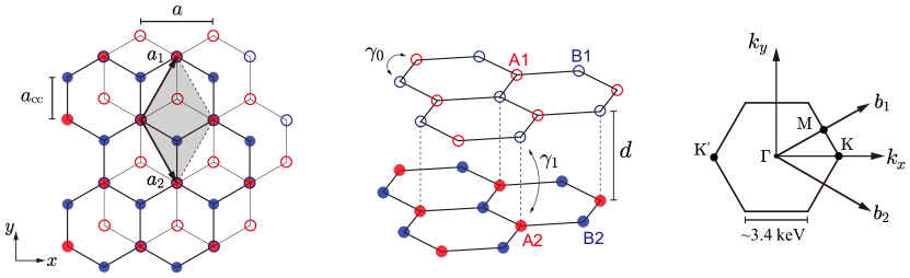
Figure 1: (Left) Crystal structure of bilayer graphene. The unit cell is highlighted in gray and contains four sublattices: A1, B1, A2, and B2. The numbers 1 and 2 represent the layer indices for the top (empty circles) and bottom (filled circles) layers, respectively. (Center) A schematic illustration of the stacking sequence for bilayer graphene with the hoppings represented by $\gamma_{0}$ and $\gamma_{1}$. The B sites of the top layer (B1) are aligned with the A sites of the bottom layer (A2). (Right) The reciprocal lattice with the reciprocal lattice vectors, and high-symmetry points $\mathrm{\Gamma},\mathrm{K},\mathrm{K^{\prime}}$, and $\mathrm{M}$ are indicated with black dots.

The low-energy band structure of the monolayer graphene is characterized by a two-dimensional massless Dirac equation with linear dispersion at two inequivalent hexagonal corners (often referred to as the valley) in the Brillouin zone, namely the $\mathrm{K}$ and $\mathrm{K}^{\prime}$ points. For a quantitative understanding of the low-energy band structure of bilayer graphene, we introduce the continuum model Hamiltonian that describes the low-energy band structure near the valley ($\mathrm{K}$ or $\mathrm{K}^{\prime}$) with the basis of four atomic sites in the unit cell (A1, B1, A2, B2):

$$H=\begin{pmatrix}\varepsilon_{\mathrm{A1}}&v\pi^{\dagger}&0&0\\ v\pi&\varepsilon_{\mathrm{B1}}&\gamma_{1}&0\\ 0&\gamma_{1}&\varepsilon_{\mathrm{A2}}&v\pi^{\dagger}\\ 0&0&v\pi&\varepsilon_{\mathrm{B2}}\end{pmatrix},$$ (2.3)

where $\pi=\xi k_{x}+ik_{y}$ is the momentum measured from the $\mathrm{K}$ ($\xi=1$) or $\mathrm{K}^{\prime}$ ($\xi=-1$) points, and $v=\sqrt{3}a\gamma_{0}/2~{}(\approx 3\times 10^{-3}$ for large $k$ within the continuum model) is the effective velocity, and $\gamma_{0}$ and $\gamma_{1}$ are the intralayer and interlayer coupling between the nearest neighbors, respectively, as described in figure 1. The diagonal terms $\varepsilon_{\mathrm{A1}}$, $\varepsilon_{\mathrm{B1}}$, $\varepsilon_{\mathrm{A2}}$, $\varepsilon_{\mathrm{B2}}$ are the on-site energies of the four atomic sites in the unit cell. Bilayer graphene consists of two stacked monolayer graphene. Thus, at the $\mathrm{K}$ and $\mathrm{K}^{\prime}$ points, there exist two copies of the Dirac Hamiltonian, originating from the top and bottom monolayer graphene sheets, which correspond to the upper-left and lower-right 2$\times$2 blocks of $H$ in eq. (2.3). Due to the interlayer coupling $\gamma_{1}$, these two Dirac Hamiltonians are coupled. This results in a pair of bands with quadratic dispersion at the Fermi energy and another pair of bands that is split away of the order of $\gamma_{1}$ from the Fermi energy, as shown in figure 2. For the hopping parameters, we used the values $\gamma_{0}=3.16\,\mathrm{eV}$ and $\gamma_{1}=0.381\,\mathrm{eV}$ [55]. More distant hoppings have a minor effect on the electronic structure, and thus exerting only a minor influence on the physics of interest in this study. Hence, we only consider the two dominant hoppings, for simplicity. As $k$ moves away from the $\mathrm{K}$ ($\mathrm{K}^{\prime}$) point ($k\gtrsim 100\,\mathrm{eV}$), the impact of $\gamma_{1}$ on the band structure diminishes. The bands start to show a linear dispersion with a band velocity $v$, similar to the monolayer case. We emphasize that the eigenenergies of the continuum model Hamiltonian in eq. (2.3) are isotropic with respect to the direction of the momentum $\boldsymbol{k}$. It is also important to note that the continuum model is valid roughly within the region where $k\lesssim 1\,\mathrm{keV}$. Beyond this limit, the system becomes anisotropic, and a tight-binding model, which is valid across the entire Brillouin zone, is required to describe the accurate behavior of the band structure, rather than a continuum model [68, 69].

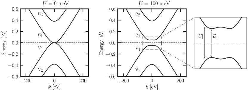
Figure 2: Band structure of bilayer graphene near the $\mathrm{K}$ or $\mathrm{K}^{\prime}$ points: without any external electric field (left) and with an external electric field (right) inducing on-site energy differences of $U=100\,\mathrm{meV}$. The dashed line represents the Fermi energy. The band structure near the Fermi energy is magnified on the right. Here, $|U|$ indicates the energy difference between the two bands labeled by c1 and v1 at the $\mathrm{K}$ or $\mathrm{K}^{\prime}$ point, and $E_{g}$ represents the band gap.

Intrinsic bilayer graphene does not have an energy gap like monolayer graphene. However, an external potential applied to bilayer graphene induces a gap [48, 57, 58]. Experimental studies have shown that, through doping or electric gating, a gap of up to approximately $300\,\mathrm{meV}$ can be achieved [59, 60]. This effect can be directly modeled from the Hamiltonian in eq. (2.3). In the presence of an external electric field perpendicular to the graphene ($\boldsymbol{E}_{\mathrm{ext}}\parallel\boldsymbol{z}$), the same potential is applied within a single layer, but the two layers experience different potentials. Denoting the potential difference between the two layers as $U$, the on-site energies become $\varepsilon_{\mathrm{A1}}=\varepsilon_{\mathrm{B1}}=U/2$ and $\varepsilon_{\mathrm{A2}}=\varepsilon_{\mathrm{B2}}=-U/2$. The band structures of BLG without and with an external potential are depicted in figure 2. The electric field opens a gap in the low-energy band structure of bilayer graphene, creating a band with a Mexican hat structure, where the band gap is given by $E_{g}=|U|\gamma_{1}/\sqrt{\gamma_{1}^{2}+U^{2}}$. For small values of $U$, the difference between $U$ and $E_{g}$ is small. For example, $E_{g}=49.6$ meV when $U=50$ meV, and $E_{g}=96.7$ meV when $U=100$ meV. However, we will not distinguish between the values of $U$ and $E_{g}$ in the rest of the paper and often use both interchangeably.

3 Dark matter-electron scattering in bilayer graphene

In this section, we describe the methods to calculate the DM scattering and absorption rates using the energy loss function of BLG.

3.1 Kinematics of dark matter

In any detector, DM scattering rate can be written as [70, 71],

$$R(t)=\frac{1}{\rho_{T}}\frac{\rho_{\chi}}{m_{\chi}}\int d\omega\int\frac{d^{3}q}{(2\pi)^{3}}\frac{\pi\sigma(q)}{\mu_{\chi e}^{2}}g(\boldsymbol{q},\omega,t)S(\boldsymbol{q},\omega).$$ (3.1)

Here, $\rho_{T}$ is the detector material density, $\rho_{\chi}$ is the local DM density that we take to be $0.4\,\mathrm{GeVcm^{-3}}$ [72], $m_{\chi}$ is the DM mass, $\sigma(q)$ is the DM-electron scattering cross section, and $\mu_{\chi e}$ is the DM-electron reduced mass. The dynamic structure factor $S(\boldsymbol{q},\omega)$ characterizes the response of the detector material for a momentum $\boldsymbol{q}$ and energy deposition $\omega$.

The scattering cross section can be split into a constant factor $\sigma_{\chi e}$ and a mediator form factor $F_{\mathrm{med}}(q)$ which is momentum-dependent, such that $\sigma(q)=\sigma_{\chi e}F_{\mathrm{med}}(q)^{2}$, where

$$\sigma_{\chi e}\equiv\dfrac{\mu_{\chi e}^{2}}{\pi}\left(\dfrac{g_{e}g_{\chi}}{q_{0}^{2}+m_{\phi}^{2}}\right)^{2}\,,\qquad F_{\mathrm{med}}(q)=\dfrac{q_{\mathrm{0}}^{2}+m_{\phi}^{2}}{q^{2}+m_{\phi}^{2}}\,.$$ (3.2)

Here, $q_{0}=\alpha m_{e}$ is a reference momentum, $m_{\phi}$ is the mediator mass, and $g_{e},g_{\chi}$ are the couplings of the mediator with electron and DM, respectively. As mentioned in section 2, we will compute the BLG response function assuming the isotropic approximation which is not valid for large $q$ and $\omega$. Hence in this paper, we will always assume a massless mediator, i.e. $q\gg m_{\phi}$.

The function $g(\boldsymbol{q},\omega,t)$ is the only time-varying quantity in eq.(3.1) and contains the directional information of the scattering rate. It is obtained by integrating the DM velocity distribution, which is assumed to be Maxwellian with a mean velocity $v_{0}=230\,\mathrm{km\,s^{-1}}$ and cut off at the local galactic escape velocity $v_{\rm esc}$. A minimum velocity $v_{-}$ is taken for a certain $q$ and $\omega$ [70, 71],

$$g(\boldsymbol{q},\omega,t)=\dfrac{2\pi^{2}v_{0}^{2}}{qN_{0}}\left[\exp\left(-\dfrac{v_{-}(\boldsymbol{q},t)^{2}}{v_{0}^{2}}\right)-\exp\left(-\dfrac{v_{\rm esc}^{2}}{v_{0}^{2}}\right)\right]\,,\quad v_{-}(\boldsymbol{q},t)=\text{min}\{v_{\mathrm{esc}},\frac{\omega}{q}+\frac{q}{2m_{\chi}}+\hat{q}\cdot\boldsymbol{v}_{\mathrm{lab}}(t)\}\,.$$ (3.3)

Here $N_{0}$ is the normalization constant of the truncated Maxwell distribution

$$N_{0}=\pi^{3/2}v_{0}^{2}\left[\mathrm{erf}\left(\frac{v_{\mathrm{esc}}}{v_{0}}\right)-\frac{2v_{\mathrm{esc}}}{\pi^{1/2}}\exp\left(-\frac{v_{\mathrm{esc}}^{2}}{v_{0}^{2}}\right)\right]\,,$$ (3.4)

and $\boldsymbol{v}_{\mathrm{lab}}(t)$ is the time-dependent velocity of the laboratory on the Earth in the galactic frame,

$$\boldsymbol{v}_{\mathrm{lab}}(t)=|\boldsymbol{v}_{E}|\begin{pmatrix}\sin\theta_{e}\sin\phi\\ \sin\theta_{e}\cos\theta_{e}(\cos\phi-1)\\ \cos^{2}\theta_{e}+\sin^{2}\theta_{e}\cos\phi\end{pmatrix}\,,$$ (3.5)

with $\phi=2\pi\times(t/24\,\mathrm{h}),\theta_{e}=42^{\circ}$, and $|\boldsymbol{v}_{E}|=240\,\mathrm{km\,s^{-1}}$. All directional information of the DM flux is included in $v_{-}(\boldsymbol{q},t)$.

The dynamic structure factor $S(\boldsymbol{q},\omega)$ can be computed in terms of the dielectric function $\varepsilon(\boldsymbol{q},\omega)$ using the fluctuation-dissipation theorem as long as the DM-electron interaction is weak [73, 74]. We describe this method in the next section.

3.2 Calculation of the dynamic structure factor

Equation (3.1) above needs to be modified appropriately as we are going to use BLG in this study, which is a 2D material. The dynamic structure factor encodes the information of the correlation of the density fluctuations in a system at a momentum $\boldsymbol{q}$ and energy $\omega$. It can be expressed using the electron density operator as the Fourier transform of the density-density correlation function [75, 76], i.e.

$$S(\boldsymbol{q},\omega)=\frac{1}{V}\int dte^{i\omega t}\langle\hat{n}(\boldsymbol{q},t)\hat{n}(-\boldsymbol{q},0)\rangle\,.$$ (3.6)

Here, $\hat{n}(\boldsymbol{q},t)$ is the electron density operator at a momentum $\boldsymbol{q}$ and time $t$:

$$\hat{n}(\boldsymbol{q},t)=\int d^{3}r\,e^{-i\boldsymbol{q}\cdot\boldsymbol{r}}\hat{n}(\boldsymbol{r},t)\,,$$ (3.7)

where $\hat{n}(\boldsymbol{r},t)$ is the electron density operator in real space. For 2D materials like BLG, the electron density is confined to the 2D space (near $r_{z}=0$). We can assume that $\hat{n}(\boldsymbol{r},t)$ can be separated into the material’s in-plane ($r_{x}$, $r_{y}$) and out-of-plane ($r_{z}$) components. Then the electron density operator can be written as

$$\hat{n}(\boldsymbol{r},t)=\hat{n}_{\mathrm{2D}}(\boldsymbol{r}_{\parallel},t)\left[\frac{1}{d}\Theta(d/2-|r_{z}|)\right].$$ (3.8)

Here, we make the assumption that the electron density remains constant between the two layers of BLG, defined within the range $-d/2<r_{z}<d/2$, where $d=3.35$ $\mathrm{\AA}$ represents the interlayer distance. The spatial coordinates in the in-plane direction are denoted as $\boldsymbol{r}_{\parallel}=(r_{x},r_{y})$, and $\Theta(x)$ represents the Heaviside step function.

Note that we have assumed a step function-like profile for the real-space electron density, as such an assumption does not significantly impact the results. Given that the DM mass is on the sub-MeV regime, the order of magnitude for $q$ is roughly in the sub-keV range, implying $qd\ll 1$. This implies that the length scale of the interlayer separation in bilayer graphene is much smaller than the inverse of the typical momentum transfer $\sim 1/q$, rendering the detailed structure of the real-space density profile less crucial for our considerations. Plugging eq. (3.8) into eq. (3.7), we get

$$\hat{n}(\boldsymbol{q},t) =\int d^{3}re^{-i\boldsymbol{q}\cdot\boldsymbol{r}}\hat{n}(\boldsymbol{r},t)$$

$$=\left[\int d^{2}r_{\parallel}e^{-i\boldsymbol{q}_{\parallel}\cdot\boldsymbol{r}_{\parallel}}n_{\mathrm{2D}}(\boldsymbol{r}_{\parallel},t)\right]\left[\int dr_{z}e^{-iq_{z}r_{z}}\frac{1}{d}\Theta(d/2-|r_{z}|)\right]$$

$$=\hat{n}_{\mathrm{2D}}(\boldsymbol{q}_{\parallel},t)\left(\frac{\sin{q_{z}d/2}}{q_{z}d/2}\right).$$ (3.9)

Using this, we can rewrite eq. (3.6) in terms of the electron density operator in 2D as

$$S(\boldsymbol{q},\omega) =\frac{1}{V}\int dte^{i\omega t}\langle\hat{n}(\boldsymbol{q},t)\hat{n}(-\boldsymbol{q},0)\rangle$$

$$=\frac{1}{d}\left(\frac{1}{A}\int dte^{i\omega t}\langle n_{\mathrm{2D}}(\boldsymbol{q}_{\parallel},t)n_{\mathrm{2D}}(-\boldsymbol{q}_{\parallel},0)\rangle\right)\left(\frac{\sin{q_{z}d/2}}{q_{z}d/2}\right)^{2}$$

$$=\frac{1}{d}S_{\mathrm{2D}}(\boldsymbol{q}_{\parallel},\omega)\left(\frac{\sin{q_{z}d/2}}{q_{z}d/2}\right)^{2},$$ (3.10)

where $V=Ad$ is the 3D volume, with $A$ being the 2D volume or surface area. Here, $S_{\mathrm{2D}}(\boldsymbol{q}_{\parallel},\omega)$ denotes the dynamic structure factor of the 2D material, and the following square of the sinc function contains the variation in the $q_{z}$-direction. Combining the aforementioned information, the detector component $\frac{1}{\rho_{T}}S(\boldsymbol{q},\omega)$ in the DM-electron scattering rate in eq. (3.1) transforms as

$$\frac{1}{\rho_{T}}S(\boldsymbol{q},\omega)\ \rightarrow\ \frac{1}{\sigma_{T}}S_{\mathrm{2D}}(\boldsymbol{q}_{\parallel},\omega)\left(\frac{\sin{q_{z}d/2}}{q_{z}d/2}\right)^{2},$$ (3.11)

where $\sigma_{T}=1.53\times 10^{-7}\mathrm{g/cm^{2}}$ is the surface density of BLG. From here on, unless otherwise specified, the dynamic structure factor will refer to $S_{\mathrm{2D}}$. Specifically, the dynamic structure factor can be written as the imaginary (dissipative) part of the 2D density-density response function $\chi_{\mathrm{2D}}(\boldsymbol{q}_{\parallel},\omega)$ derived from the fluctuation-dissipation theorem [75, 76]:

$$S_{\mathrm{2D}}(\boldsymbol{q}_{\parallel},\omega)=-\frac{2}{1-e^{-\beta\omega}}\mathrm{Im}\left[\chi_{\mathrm{2D}}(\boldsymbol{q}_{\parallel},\omega)\right],$$ (3.12)

where $\beta=1/(k_{B}T)$. The 2D density-density response function in the frequency-momentum space is the Fourier transform of the 2D retarded density correlation function given by

$$\chi_{\mathrm{2D}}(\boldsymbol{q}_{\parallel},\omega)=-\frac{i}{A}\int dte^{i\omega t}\left<\left[\hat{n}_{\mathrm{2D}}(\boldsymbol{q}_{\parallel},t),\hat{n}_{\mathrm{2D}}(-\boldsymbol{q}_{\parallel},0)\right]\right>.$$ (3.13)

Note that the expectation value $\langle\cdots\rangle$ refers to the thermal average over many-body states, taking into account the Coulomb interaction between the electrons. It is often practical to introduce the dielectric function of the detector. The dielectric function, in the frequency-momentum space, is defined as the ratio of the screened potential to the bare potential in a material. The 2D version of the dielectric function is given by

$$\frac{1}{\varepsilon(\boldsymbol{q}_{\parallel},\omega)}=1+v_{\mathrm{C}}(\boldsymbol{q}_{\parallel})\chi_{\mathrm{2D}}(\boldsymbol{q}_{\parallel},\omega)\,,$$ (3.14)

where $v_{\mathrm{C}}(q)=\dfrac{e^{2}}{2\varepsilon_{r}q}$ is the 2D Coulomb interaction. Here, $\varepsilon_{r}$ is the dielectric constant of the medium which we assume to be a vacuum. At zero temperature, the dynamic structure factor in eq. (3.12) becomes

$$S_{\mathrm{2D}}(\boldsymbol{q}_{\parallel},\omega)=-2\Theta(\omega)\mathrm{Im}\chi_{\mathrm{2D}}(\omega)=\frac{2\Theta(\omega)}{v_{\mathrm{C}}(\boldsymbol{q}_{\parallel})}\mathcal{W}(\boldsymbol{q}_{\parallel},\omega),\quad\mathcal{W}(\boldsymbol{q}_{\parallel},\omega)=\mathrm{Im}\left[-\frac{1}{\varepsilon(\boldsymbol{q}_{\parallel},\omega)}\right].$$ (3.15)

This implies a direct connection between the dynamic structure factor and the imaginary part of the inverse dielectric function, termed the energy loss function (ELF) $\mathcal{W}(\boldsymbol{q},\omega)$. The ELF represents electronic energy loss in materials and is thus related to an experimentally measurable quantity. The information about the response to a small density perturbation is contained in the dielectric function.

To calculate the ELF, we can use the random phase approximation (RPA) to compute the expectation value in eq. (3.13). Diagrammatically, the RPA corresponds to an infinite series of the non-interacting polarization function connected by the Coulomb interaction lines, neglecting other higher-order terms [77, 78, 75, 76]:

$$\chi_{\mathrm{2D}}(\boldsymbol{q}_{\parallel},\omega)=\frac{\chi_{\mathrm{2D}}^{(0)}(\boldsymbol{q}_{\parallel},\omega)}{\varepsilon(\boldsymbol{q}_{\parallel},\omega)}\,,\quad\varepsilon(\boldsymbol{q}_{\parallel},\omega)=1-v_{\mathrm{C}}(\boldsymbol{q}_{\parallel})\chi_{\mathrm{2D}}^{(0)}(\boldsymbol{q}_{\parallel},\omega)\,,$$ (3.16)

where the response function in eq. (3.13) and the dielectric function in eq. (3.14) are expressed in terms of the non-interacting polarization function $\chi^{(0)}_{\mathrm{2D}}(\boldsymbol{q},\omega)$ using the RPA. This approach is known to be valid in the weak coupling (typically high density) limit or in the large fermion flavor limit. $\chi^{(0)}_{\mathrm{2D}}(\boldsymbol{q},\omega)$ is given by [75]

$$\chi^{(0)}_{\mathrm{2D}}(\boldsymbol{q}_{\parallel},\omega)=g\sum_{n,m}\int\frac{d^{2}k}{(2\pi)^{2}}\frac{f_{\boldsymbol{k},n}-f_{\boldsymbol{k}+\boldsymbol{q}_{\parallel},m}}{\omega+\varepsilon_{\boldsymbol{k},n}-\varepsilon_{\boldsymbol{k}+\boldsymbol{q}_{\parallel},m}+i\eta}|\langle\boldsymbol{k},n|\boldsymbol{k}+\boldsymbol{q}_{\parallel},m\rangle|^{2},$$ (3.17)

where $\varepsilon_{\boldsymbol{k},n}$ and $f_{\boldsymbol{k},n}=1/[1+e^{\beta(\varepsilon_{\boldsymbol{k},n}-\mu)}]$ are the eigenenergy and the Fermi-Dirac distribution for the wave vector $\boldsymbol{k}$ and band index $n$, respectively, $g=4$ is the spin-valley degeneracy factor for graphene, and $\mu$ is the chemical potential, $\eta$ is a phenomenological broadening parameter proportional to the inverse lifetime (or decay width) of quasiparticles which takes $\eta\rightarrow 0^{+}$ for the clean limit. For numerical calculations, we set $\eta=1$ meV, which is the typical order of magnitude for BLG [79, 80, 81]. We note that variations in $\eta$ have a negligible impact on the overall results.

In this work, we will also consider DM absorption in BLG. To this end, we will show the results for a dark photon model where the DM mixes with the Standard Model (SM) photon through a small mixing parameter $\kappa$,

$$\mathcal{L}\supset\kappa F_{\mu\nu}F^{\prime\mu\nu}\,,$$ (3.18)

where $F^{\mu\nu}$ and $F^{\prime\mu\nu}$ are the field strengths of the SM photon and the dark photon, respectively. Because of the mixing between dark photon DM and the Standard Model photon, DM absorption rate is again related to the ELF of the material rescaled by the mixing parameter $\kappa$ as follows [82],

$$R_{\rm abs}=\kappa^{2}\rho_{\chi}\dfrac{d}{\sigma_{T}}\,\mathrm{Im}\left[-\frac{1}{\varepsilon(q,\omega)}\right]\,,$$ (3.19)

with $\omega=m_{\chi}$ and $q=m_{\chi}v$. Because $q\ll\omega$ for DM absorption, it is more convenient to calculate the dielectric function in 2D using the following expression [83, 78]

$$\varepsilon(q\rightarrow 0,\omega)=1+\dfrac{i}{2\varepsilon_{r}}\dfrac{q}{\omega}\sigma(\omega).$$ (3.20)

Here $\varepsilon_{r}$ denotes the dielectric constant of the medium which we assume to be vacuum, and the optical conductivity $\sigma(\omega)$ of BLG is calculated using the Kubo formula [77]. We will show projection of constraint on the mixing parameter $\kappa$.

4 Results

We now have all the tools needed to calculate the ELF of BLG, and the DM scattering and absorption rates. In this section, we will show and explain our main results.

4.1 Dielectric properties of bilayer graphene

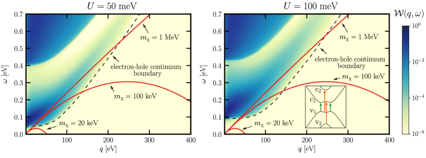
Figure 3: The color plot of the energy loss function (ELF) for BLG with $U=50\,\mathrm{meV}$ (left) and $100\,\mathrm{meV}$ (right), represented in the $q$ - $\omega$ plane. The black dashed line indicates the boundary of the electron-hole continuum, with the more intensely colored region above signifying the continuum itself. The kinematically-allowed boundaries for DM with mass $m_{\chi}=20,100$, and $1000\,\mathrm{keV}$ are depicted by the red solid lines. The inset in the right panel figure shows the different electronic transitions that give rise to the features of the ELF. See section 4.1 for more details.

The ELF of BLG in the presence of a potential, calculated through eqs. (3.15)-(3.17), is shown as a color plot in the $q$ - $\omega$ plane in figure 3. Since the low-energy band structure described by the continuum model Hamiltonian in eq. (2.3) is isotropic, the ELF also depends only on the magnitude of $\boldsymbol{q}$ and not on its direction.

The magnitude of the ELF is related to the electronic energy loss at the momentum transfer $q$ and energy transfer $\omega$. Especially when there is a gap and the Fermi energy lies within it, the origin of the ELF is the interband transitions of electrons. This represents cases where momentum transfer by $q$ and energy transfer by $\omega$ are possible from an occupied band to an empty band, and this region is referred to as the electron-hole continuum [75]. For example, in the region where $\omega<E_{g}$, the ELF is close to zero, which means the absence of available states for excitation below the gap. The boundary of the electron-hole continuum is indicated by a dashed line in figure 3. Additionally, for $q\gtrsim 100\,\mathrm{keV}$, the boundary of the electron-hole continuum in $q$ - $\omega$ plane shows a linear dispersion with the velocity $v$ in eq. (2.3). We note that since the Fermi energy lies within the gap, implying no states exist at that energy, contributions from intraband transitions or plasmons to the ELF are absent in this case.

The red curves indicate the kinematic phase space of DM of mass $m_{\chi}$. Here, the mean DM velocity is assumed to be $v_{0}=230\,\mathrm{km\,s^{-1}}$. In the phase space where there is an overlap between this kinematically-allowed region and the dark areas of the BLG’s ELF, DM-electron scattering occurs. If there is no overlap, the scattering rate vanishes. For example, in the case where $m_{\chi}=20\,\mathrm{keV}$, the kinematically-allowed region exists outside the electron-hole continuum, leading to no DM-electron scattering. This means that the $U$ applied to the BLG determines the minimum detectable mass threshold for DM. The continuum model we employed is valid for ranges approximately $q\lesssim 1\,\mathrm{keV}$ and $\omega\lesssim 2\,\mathrm{eV}$. For DM with a mass $m_{\chi}=1\,\mathrm{MeV}$, the kinematically-allowed boundary extends into regions with $q>1\,\mathrm{keV}$. However, the region contributing to the DM-electron scattering rate, that is, the area overlapping with the electron-hole continuum, is approximately $q\lesssim 0.6\,\mathrm{keV}$. Therefore, the description using the continuum model Hamiltonian remains valid. Consequently, our results are relevant for DM mass range up to approximately $m_{\chi}\lesssim 1\,\mathrm{MeV}$.

For larger values of $m_{\chi}$, a tight-binding model that is valid across the entire Brillouin zone is required, rather than a continuum model. Then the band structure no longer remains isotropic in the momentum space, leading to the loss function developing a directional dependence on $\boldsymbol{q}$. Additionally, when the magnitude of the $q$ exceeds the size of the Brillouin zone, considerations like the local field effects [75, 84] become necessary in the determination of the dielectric function. On the low mass end, we are limited by the finite value of $U$. Energy deposition below $U$ is not possible which will help reduce the thermal fluctuations.

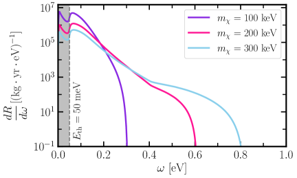
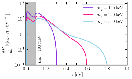
Figure 4: Energy spectrum of DM scattering rate in bilayer graphene with two band gaps $U=50\,\mathrm{meV}$ (left) and $100\,\mathrm{meV}$ (right) for $m_{\chi}=100$ (violet), 200 (pink), and $300\,\mathrm{keV}$ (sky blue). A massless mediator and $\sigma_{\chi e}=10^{-38}\,\mathrm{cm^{2}}$ are assumed in all cases. The energy thresholds are marked with a vertical gray line. The gray-shaded below-threshold regions are not taken into account in our results.

Having discussed the properties of the ELF of bilayer graphene, we now compute the DM scattering rate following eq. (3.1). We show the scattering rate as a function of energy in figure 4 for $m_{\chi}=100,200,$ and $300\,\mathrm{keV}$ for two values of $U=50,100\,\mathrm{meV}$ and cross section $\sigma_{\chi e}=10^{-38}\,\mathrm{cm^{2}}$. These thresholds are marked with a vertical gray line. As mentioned before, we will only show results for the massless mediator case. From figure 4, we can see that the rates are maximum near the thresholds and decreases toward higher energies. This maximum rate comes from the electronic transitions from the valence to the conduction bands $v_{1}\to c_{1}$ as shown in the inset in the right panel of figure 3 (green arrows). Moreover, the overall rate increases for heavier DM. This is understandable from the overlap between the DM kinematic phase space and the ELF of BLG in the $q$ - $\omega$ plane in figure 3. For low mass DM, the overlap region is small and limited toward the low energy corner of the plane, hence the scattering rate is maximum around $E_{g}$. For heavier mass, the overlap region is extended to higher energies and has support from the additional $v_{1}\to c_{2}$ and $v_{2}\to c_{1}$ electronic transitions marked with the orange arrows in the inset of figure 3. This broadens the spectrum toward higher energy for heavier mass DM as can be seen in figure 4. Finally, we note that the rates are higher for the case $E_{g}=50\,\mathrm{meV}$ because the ELF in this case peaks at a relatively lower energy ($v_{1}\to c_{1}$ transition) yielding a greater overlap with the DM kinematic phase space. This is also evident from figure 3, indicating that the sensitivity could further improve for smaller $E_{g}$. However, a smaller value of $E_{g}$ will also be subject to the technical challenge of maintaining the same gate voltage over a large volume of the target. The optimal value of $E_{g}$ will thus depend on the details of the experimental design.

Before ending this section, we want to comment on the additional below-threshold peaks that appear in the gray-shaded region in figure 4. These are arising from the small but nonzero value of the ELF in the $\omega<E_{g}$ energy regime which, in turn, is a result of our assumption of a nonzero decay width $\eta$ of the excited electron-hole pairs in eq. (3.17). This small value of the ELF, combined with the diverging nature of the form factor $F_{\mathrm{med}}(q)\propto 1/q^{2}$ at small $q$, gives rise to these additional peaks. However, we note that if $\eta$ were zero, the ELF would completely vanish below $\omega<E_{g}$, resulting in a zero value of $dR/d\omega$ in this energy range. In our calculation, we do not include the energy range below $\omega<E_{g}=E_{\mathrm{th}}$, and assume the thresholds to be the same as the band gap in each case.

4.2 Projected sensitivity & daily modulation

In this section, we will explore the future projections with bilayer graphene as the detector to search for DM. We envisage an experimental setup similar to the ones developed for photon detectors with monolayer and bilayer graphene [85, 86, 87, 88, 89, 90]. Graphene being an atomic-thick material, one needs a relatively large surface area to achieve a reasonable amount of detector mass. One way is to prepare multiple sheets of BLG and build a single detector module. A single experiment then can deploy multiple such modules to achieve larger target mass. In this regard, we want to mention about an upcoming experiment called PTOLEMY that is planning to use tritium adsorbed onto graphene substrate to detect low energy cosmic neutrinos [91, 92]. The technical design of a BLG DM detector can get help from PTOLEMY’s prototype detector design and background study as their goal is also to achieve a large exposure ($\sim$ 100 g-yr). To reach the desirable energy threshold, the BLG needs to be biased with the appropriate voltage, and the setup needs to be cooled down below that temperature to mitigate the background noise from thermal fluctuations. Moreover, the excited electron-hole pairs created from DM scattering and absorption need to be detected. This can be done with sensitive charge detectors similar to the charge-coupled devices [93, 94]. In this paper, we do not go into any further technical detail about the experimental setup and leave it for future work.

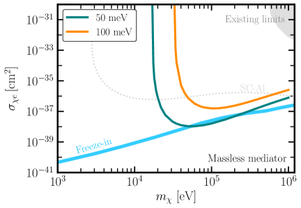
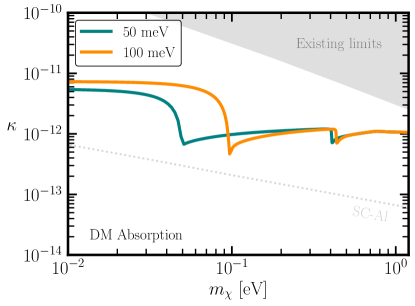
Figure 5: Projected sensitivties on DM-electron scattering cross section $\sigma_{\chi e}$ (left) and DM mixing parameter $\kappa$ for absorption (right) in bilayer graphene with two energy thresholds $E_{\mathrm{th}}=50$ and $100\,\mathrm{meV}$ assuming 3 events in 10 mg-yr exposure with no background. We use scattering rate averaged over a 24 hour period. The blue band marked with ‘Freeze-in’ in the left panel is the region of theoretical interest. For comparison, we also show the projection for superconducting aluminum (SC-Al) as a gray, dotted line [95]. Bilayer graphene is superior to superconducting aluminum for DM scattering in the $20\,\mathrm{keV}-\,\mathrm{MeV}$ mass range. The dips appearing for the DM absorption sensitivity curve in the right panel are due to opening up of different band transitions of electrons. See the text for more details. The gray-shaded regions are excluded by other laboratory and astrophysical constraints [14, 96, 10, 97, 98, 99, 100].

We show the projected sensitivity for DM-electron scattering in the left panel for the case of a massless mediator, and DM absorption in the right panel of figure 5. As mentioned before, we show the results for two values of $U=50\,\mathrm{meV}$ (orange) and $100\,\mathrm{meV}$ (teal) assuming a cutoff of 3 events for an exposure of 10 mg-yr for both cases with no background. We lose sensitivity below $m_{\chi}\simeq 20$ and $35\,\mathrm{keV}$, respectively, for the two band gaps which can be understood from their respective energy thresholds. For comparison, we also show the projection for superconducting aluminum as a gray, dotted line [95]. The left panel of figure 5 shows that BLG performs better than superconducting aluminum for DM scattering in the $10\,\mathrm{keV}-\,\mathrm{MeV}$ mass range for the same amount of exposure. With the assumed 3 events per 10 mg-yr exposure limit, BLG sensitivity can reach $\sigma_{\chi e}\simeq 10^{-38}\,\mathrm{cm^{2}}$ for $m_{\chi}\simeq 60\,\mathrm{keV}$, and hence, the band of freeze-in benchmark model marked with blue in figure 5.

In the case of DM absorption, we show our sensitivity projections on the mixing parameter $\kappa$ of dark photon DM in the mass range $0.01<m_{\chi}<1\,\mathrm{eV}$ as the whole DM mass energy is absorbed ($\omega=m_{\chi}$). It is computed using eq. (3.19) and the same limit 3 events per 10 mg-yr exposure with no background. We see that the sensitivity can reach $\kappa\simeq 10^{-12}$ as shown in the right panel of figure 5. The dips in the DM absorption sensitivity curve are coming from the opening up of electronic transitions between different bands, such as $v_{1}\to c_{1}$, $v_{1}\to c_{2}$, or $v_{2}\to c_{1}$, in the ELF as was discussed in section 4.1. The gray-shaded regions are excluded by existing laboratory and astrophysical constraints [14, 96, 10, 97, 98, 99, 100]. We computed the sensitivity of BLG for pseudoscalar DM absorption too which is also related to the conductivity [82]. However, we do not show it here as it does not reach a coupling strength that is not already constrained by other astrophysical observations.

Another important characteristic of a BLG detector is the daily modulation of the DM scattering rate. This arises from the change in the direction of the incoming DM wind due to the rotation of the Earth about its axis. The two-dimensional nature of BLG facilitates the daily modulation even more as it makes the detector response $S(\boldsymbol{q},\omega)$ inherently anisotropic. The time modulation information in the scattering rate is included in the $g(\boldsymbol{q},\omega,t)$ factor in eq.(3.1). In figure 6, we show the daily modulation of the scattering rate normalized by the average $R(t)/\langle R\rangle$ over a 24 hr period for a few DM masses in BLG with $U=100\,\mathrm{meV}$. The rate varies by upto $R(t)/\langle R\rangle\simeq 80\%$ for $m_{\chi}=120\,\mathrm{keV}$ and by smaller amount for heavier DM mass. The amount of modulation is more for lighter DM mass. This is understandable as the typical energy transfer is closer to the threshold for lighter DM and a small change in the relative velocity of DM can affect the scattering rate significantly. Such daily modulation of DM scattering rate can be leveraged to isolate any potential DM signal in a future experiment from various background scattering events from cosmic rays, radioactivity, or any internal systematic noise that do not share such time variation. We note that on top of the daily modulation, there is also an annual modulation expected from the rotation of the Earth around the sun resulting in a slightly different relative velocities of the DM wind throughout the year. We do not calculate it in this work.

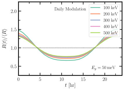
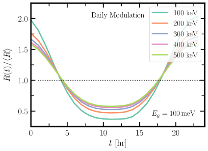
Figure 6: Daily modulation of the scattering rate of a few DM masses in bilayer graphene with $E_{g}=50$ (left) and $100\,\mathrm{meV}$ (right). The modulation is more pronounced for lighter DM as the typical energy transfer is closer to the threshold, and it is milder for lower threshold $50\,\mathrm{meV}$ compared to $100\,\mathrm{meV}$ due to the same reason.

In passing, we want to point out that the DM in the Milky Way halo may have a kinematic substructure in the solar neighborhood with a different density and velocity distribution. In such a case, the sensitivity projections and the daily modulation may get affected because of the substructure [101, 102].

5 Conclusions & Outlook

In this paper, we proposed bilayer graphene (BLG) as a target material for DM direct detection experiment and studied its sensitivity to probe DM-ordinary matter interaction. BLG is a 2D material consisting of two honeycomb lattices of carbon atoms stacked together. The electrons in a BLG possess a tunable band gap that can be adjusted with a gate voltage applied across the material. This band gap can be used as the energy threshold in the experiment giving us a convenient control on the thermal noise background. We computed the dielectric function of BLG using the random phase approximation and used it to compute the DM scattering and absorption rates. We then showed projections for limits on the DM-electron scattering cross section $\sigma_{\chi e}$ for a massless mediator, and on the kinetic mixing parameter $\kappa$ between dark photon DM and ordinary photon. Our results show that a 10 mg-yr experimental exposure with no background will allow us to probe $\sigma_{\chi e}\gtrsim 10^{-38}\,\mathrm{cm^{2}}$ around $m_{\chi}\simeq 50\,\mathrm{keV}$, and reach the freeze-in benchmark models in the DM-electron scattering parameter space. Thanks to the small value of the band gap, BLG can detect $\sim 20\,\mathrm{keV}$ mass DM, and potentially even reach below $10\,\mathrm{keV}$ if lower energy threshold is achievable. Such small energy threshold may also allow us to probe the very low energy Earth-bound thermalized DM population predicted by some models. In the context of a dark photon model, DM absorption in BLG can probe $\kappa\gtrsim 10^{-12}$ in the sub-eV mass range. We also compute the expected daily modulation in the DM scattering rate due to the rotation of the Earth about its axis. We found that the scattering rate can vary by upto $\sim 80\%$ from the average value for lighter DM. This modulation can help us distinguish the DM signal from other constant background sources.

The promising results from this study motivates us to ask next - how to build a DM detector using BLG? A detailed and more dedicated study is required to answer this question. We plan to pursue that in a future work. In this regard, we pointed out the future experiment called PTOLEMY that is planning to detect low energy cosmic neutrinos using tritium adsorbed on graphene layers. Perhaps, a future experiment using BLG can get technical help from PTOLEMY as their aim is to achieve an ambitious 100 g-yr exposure [91, 103, 92]. In the projection calculation of this paper, we did not assume any background. However, in reality one should expect various sources of backgrounds, such as cosmic rays, radioactive sources, thermal noise etc. The muons and gamma rays from the cosmic rays can be mitigated by doing the experiment in an underground laboratory. The environmental radioactive sources are more difficult to get rid of. Appropriate shielding of the experimental setup and careful modeling of the remaining radioactive sources is one solution. Additionally, there could be hardware-specific systematics that one might need to pay attention to [35].

Both, direct detection of sub-MeV DM and graphene are relatively new areas of research with many novel ideas being developed today. Hence, there are plenty of scopes to improve the idea presented in this paper. For example, figure 3 clearly tells us that the sensitivity of bilayer graphene as DM target can be further improved by matching its band velocity $v$ with the DM velocity, or by extending the overlap between the detector response and DM phase space using flatter bands. Twisted bilayer [63, 64, 65, 66] or multilayer ($>2$) graphene [104, 105] could be useful for this purpose. Recent research has seen significant progress in studying flat band materials, where the bands near the Fermi level exhibit flat characteristics [106]. Various materials, such as the kagome lattice, have been discovered [107, 108]. Such flat band materials can offer improvement in the sensitivity of DM detectors. We want to pursue these possibilities in future.

References

- [1] Y. Hochberg, E. Kuflik, T. Volansky and J.G. Wacker, Mechanism for Thermal Relic Dark Matter of Strongly Interacting Massive Particles, Phys. Rev. Lett. 113 (2014) 171301 [1402.5143].
- [2] C. Boehm, P. Fayet and J. Silk, Light and heavy dark matter particles, Phys. Rev. D 69 (2004) 101302 [hep-ph/0311143].
- [3] C. Boehm and P. Fayet, Scalar dark matter candidates, Nucl. Phys. B 683 (2004) 219 [hep-ph/0305261].
- [4] P. Fayet, Light spin 1/2 or spin 0 dark matter particles, Phys. Rev. D 70 (2004) 023514 [hep-ph/0403226].
- [5] E. Izaguirre, G. Krnjaic, P. Schuster and N. Toro, Analyzing the Discovery Potential for Light Dark Matter, Phys. Rev. Lett. 115 (2015) 251301 [1505.00011].
- [6] J.H. Chang, R. Essig and A. Reinert, Light(ly)-coupled Dark Matter in the keV Range: Freeze-In and Constraints, JHEP 03 (2021) 141 [1911.03389].
- [7] R.T. D’Agnolo, C. Mondino, J.T. Ruderman and P.-J. Wang, Exponentially Light Dark Matter from Coannihilation, JHEP 08 (2018) 079 [1803.02901].
- [8] CRESST collaboration, Results on MeV-scale dark matter from a gram-scale cryogenic calorimeter operated above ground, Eur. Phys. J. C 77 (2017) 637 [1707.06749].
- [9] CRESST collaboration, First results from the CRESST-III low-mass dark matter program, Phys. Rev. D 100 (2019) 102002 [1904.00498].
- [10] SuperCDMS collaboration, Light Dark Matter Search with a High-Resolution Athermal Phonon Detector Operated Above Ground, Phys. Rev. Lett. 127 (2021) 061801 [2007.14289].
- [11] R. Ren et al., Design and characterization of a phonon-mediated cryogenic particle detector with an eV-scale threshold and 100 keV-scale dynamic range, Phys. Rev. D 104 (2021) 032010 [2012.12430].
- [12] CPD collaboration, Performance of a large area photon detector for rare event search applications, Appl. Phys. Lett. 118 (2021) 022601 [2009.14302].
- [13] “The TESSERACT dark matter project, SNOWMASS LOI.” www.snowmass21.org/docs/files/summaries/CF/SNOWMASS21-CF1_CF2-IF1_IF8-120.pdf.
- [14] SENSEI collaboration, SENSEI: Direct-Detection Results on sub-GeV Dark Matter from a New Skipper-CCD, Phys. Rev. Lett. 125 (2020) 171802 [2004.11378].
- [15] DAMIC-M collaboration, First Constraints from DAMIC-M on Sub-GeV Dark-Matter Particles Interacting with Electrons, Phys. Rev. Lett. 130 (2023) 171003 [2302.02372].
- [16] Oscura collaboration, The Oscura Experiment, 2202.10518.
- [17] S. Rajendran, N. Zobrist, A.O. Sushkov, R. Walsworth and M. Lukin, A method for directional detection of dark matter using spectroscopy of crystal defects, Phys. Rev. D 96 (2017) 035009 [1705.09760].
- [18] M.C. Marshall, M.J. Turner, M.J.H. Ku, D.F. Phillips and R.L. Walsworth, Directional detection of dark matter with diamond, Quantum Sci. Technol. 6 (2021) 024011 [2009.01028].
- [19] S.A. Hertel, A. Biekert, J. Lin, V. Velan and D.N. McKinsey, Direct detection of sub-GeV dark matter using a superfluid 4He target, Phys. Rev. D 100 (2019) 092007 [1810.06283].
- [20] H.J. Maris, G.M. Seidel and D. Stein, Dark Matter Detection Using Helium Evaporation and Field Ionization, Phys. Rev. Lett. 119 (2017) 181303 [1706.00117].
- [21] R. Anthony-Petersen et al., Applying Superfluid Helium to Light Dark Matter Searches: Demonstration of the HeRALD Detector Concept, 2307.11877.
- [22] G.-B. Kim, Self-absorption and Phonon Pulse Shape Discrimination in Scintillating Bolometers, J. Low Temp. Phys. 199 (2020) 1004.
- [23] Y. Hochberg, Y. Zhao and K.M. Zurek, Superconducting Detectors for Superlight Dark Matter, Phys. Rev. Lett. 116 (2016) 011301 [1504.07237].
- [24] Y. Hochberg, I. Charaev, S.-W. Nam, V. Verma, M. Colangelo and K.K. Berggren, Detecting Sub-GeV Dark Matter with Superconducting Nanowires, Phys. Rev. Lett. 123 (2019) 151802 [1903.05101].
- [25] J. Chiles et al., New Constraints on Dark Photon Dark Matter with Superconducting Nanowire Detectors in an Optical Haloscope, Phys. Rev. Lett. 128 (2022) 231802 [2110.01582].
- [26] Y.-H. Kim, S.-J. Lee and B. Yang, Superconducting detectors for rare event searches in experimental astroparticle physics, Superconductor Science and Technology 35 (2022) 063001.
- [27] A. Das, N. Kurinsky and R.K. Leane, Dark Matter Induced Power in Quantum Devices, 2210.09313.
- [28] C.W. Fink, C.P. Salemi, B.A. Young, D.I. Schuster and N.A. Kurinsky, The Superconducting Quasiparticle-Amplifying Transmon: A Qubit-Based Sensor for meV Scale Phonons and Single THz Photons, 2310.01345.
- [29] Z.-L. Liang, C. Mo, F. Zheng and P. Zhang, Phonon-mediated Migdal effect in semiconductor detectors, Phys. Rev. D 106 (2022) 043004 [2205.03395].
- [30] Y. Hochberg, Y. Kahn, M. Lisanti, K.M. Zurek, A.G. Grushin, R. Ilan et al., Detection of sub-MeV Dark Matter with Three-Dimensional Dirac Materials, Phys. Rev. D 97 (2018) 015004 [1708.08929].
- [31] R.M. Geilhufe, F. Kahlhoefer and M.W. Winkler, Dirac Materials for Sub-MeV Dark Matter Detection: New Targets and Improved Formalism, Phys. Rev. D 101 (2020) 055005 [1910.02091].
- [32] Z. Huang, C. Lane, S.E. Grefe, S. Nandy, B. Fauseweh, S. Paschen et al., Dark Matter Detection with Strongly Correlated Topological Materials: Flatband Effect, 2305.19967.
- [33] C. Blanco, R. Essig, M. Fernandez-Serra, H. Ramani and O. Slone, Dark matter direct detection with quantum dots, Phys. Rev. D 107 (2023) 095035 [2208.05967].
- [34] R. Essig, G.K. Giovanetti, N. Kurinsky, D. McKinsey, K. Ramanathan, K. Stifter et al., Snowmass2021 Cosmic Frontier: The landscape of low-threshold dark matter direct detection in the next decade, in Snowmass 2021, 3, 2022 [2203.08297].
- [35] P. Adari et al., EXCESS workshop: Descriptions of rising low-energy spectra, SciPost Phys. Proc. 9 (2022) 001 [2202.05097].
- [36] A. Gould and G. Raffelt, Thermal Conduction by Massive Particles, Astrophys. J. 352 (1990) 654.
- [37] H. Banks, S. Ansari, A.C. Vincent and P. Scott, Simulation of energy transport by dark matter scattering in stars, JCAP 04 (2022) 002 [2111.06895].
- [38] V. De Luca, A. Mitridate, M. Redi, J. Smirnov and A. Strumia, Colored Dark Matter, Phys. Rev. D 97 (2018) 115024 [1801.01135].
- [39] B. Dasgupta, A. Gupta and A. Ray, Dark matter capture in celestial objects: light mediators, self-interactions, and complementarity with direct detection, JCAP 10 (2020) 023 [2006.10773].
- [40] M. Pospelov and H. Ramani, Earth-bound millicharge relics, Phys. Rev. D 103 (2021) 115031 [2012.03957].
- [41] R.K. Leane and J. Smirnov, Floating dark matter in celestial bodies, JCAP 10 (2023) 057 [2209.09834].
- [42] S. Baum, L. Visinelli, K. Freese and P. Stengel, Dark matter capture, subdominant WIMPs, and neutrino observatories, Phys. Rev. D 95 (2017) 043007 [1611.09665].
- [43] S. Rajendran and H. Ramani, Composite solution to the neutron lifetime anomaly, Phys. Rev. D 103 (2021) 035014 [2008.06061].
- [44] D. Budker, P.W. Graham, H. Ramani, F. Schmidt-Kaler, C. Smorra and S. Ulmer, Millicharged Dark Matter Detection with Ion Traps, PRX Quantum 3 (2022) 010330 [2108.05283].
- [45] J. Billard, M. Pyle, S. Rajendran and H. Ramani, Calorimetric Detection of Dark Matter, 2208.05485.
- [46] D. McKeen, M. Moore, D.E. Morrissey, M. Pospelov and H. Ramani, Accelerating Earth-Bound Dark Matter, 2202.08840.
- [47] D. McKeen, D.E. Morrissey, M. Pospelov, H. Ramani and A. Ray, Dark Matter Annihilation inside Large-Volume Neutrino Detectors, Phys. Rev. Lett. 131 (2023) 011005 [2303.03416].
- [48] A.H. Castro Neto, F. Guinea, N.M.R. Peres, K.S. Novoselov and A.K. Geim, The electronic properties of graphene, Reviews of Modern Physics 81 (2009) 109 [0709.1163].
- [49] S.-Y. Wang, Graphene-based detectors for directional dark matter detection, Eur. Phys. J. C 79 (2019) 561 [1509.08801].
- [50] Y. Hochberg, Y. Kahn, M. Lisanti, C.G. Tully and K.M. Zurek, Directional detection of dark matter with two-dimensional targets, Phys. Lett. B 772 (2017) 239 [1606.08849].
- [51] D. Kim, J.-C. Park, K.C. Fong and G.-H. Lee, Detection of Super-light Dark Matter Using Graphene Sensor, 2002.07821.
- [52] R. Catena, T. Emken, M. Matas, N.A. Spaldin and E. Urdshals, Direct searches for general dark matter-electron interactions with graphene detectors: Part II. Sensitivity studies, 2303.15509.
- [53] R. Catena, T. Emken, M. Matas, N.A. Spaldin and E. Urdshals, Direct searches for general dark matter-electron interactions with graphene detectors: Part I. Electronic structure calculations, 2303.15497.
- [54] E.V. Castro, N.M.R. Peres, J.M.B. Lopes dos Santos, F. Guinea and A.H. Castro Neto, Bilayer graphene: gap tunability and edge properties, in Journal of Physics Conference Series, vol. 129 of Journal of Physics Conference Series, p. 012002, Oct., 2008, DOI [1004.5079].
- [55] E. McCann and M. Koshino, The electronic properties of bilayer graphene, Reports on Progress in Physics 76 (2013) 056503 [1205.6953].
- [56] A.V. Rozhkov, A.O. Sboychakov, A.L. Rakhmanov and F. Nori, Electronic properties of graphene-based bilayer systems, Phys. Rep. 648 (2016) 1 [1511.06706].
- [57] E. McCann, Asymmetry gap in the electronic band structure of bilayer graphene, Phys. Rev. B 74 (2006) 161403.
- [58] H. Min, B. Sahu, S.K. Banerjee and A.H. MacDonald, Ab initio theory of gate induced gaps in graphene bilayers, Phys. Rev. B 75 (2007) 155115.
- [59] J.B. Oostinga, H.B. Heersche, X. Liu, A.F. Morpurgo and L.M.K. Vandersypen, Gate-induced insulating state in bilayer graphene devices, Nature Materials 7 (2008) 151.
- [60] E.V. Castro, K.S. Novoselov, S.V. Morozov, N.M.R. Peres, J.M.B.L. dos Santos, J. Nilsson et al., Biased bilayer graphene: Semiconductor with a gap tunable by the electric field effect, Phys. Rev. Lett. 99 (2007) 216802.
- [61] Z. Liu, K. Suenaga, P.J.F. Harris and S. Iijima, Open and closed edges of graphene layers, Phys. Rev. Lett. 102 (2009) 015501.
- [62] P.L. de Andres, R. Ramírez and J.A. Vergés, Strong covalent bonding between two graphene layers, Phys. Rev. B 77 (2008) 045403.
- [63] R. Bistritzer and A.H. MacDonald, Moiré bands in twisted double-layer graphene, Proceedings of the National Academy of Sciences 108 (2011) 12233.
- [64] Y. Cao, V. Fatemi, S. Fang, K. Watanabe, T. Taniguchi, E. Kaxiras et al., Unconventional superconductivity in magic-angle graphene superlattices, Nature 556 (2018) 43 [1803.02342].
- [65] Y. Cao, V. Fatemi, A. Demir, S. Fang, S.L. Tomarken, J.Y. Luo et al., Correlated insulator behaviour at half-filling in magic-angle graphene superlattices, Nature 556 (2018) 80.
- [66] E.Y. Andrei and A.H. MacDonald, Graphene bilayers with a twist, Nature Materials 19 (2020) 1265.
- [67] T. Ohta, A. Bostwick, T. Seyller, K. Horn and E. Rotenberg, Controlling the electronic structure of bilayer graphene, Science 313 (2006) 951 [https://www.science.org/doi/pdf/10.1126/science.1130681].
- [68] E. McCann and M. Koshino, The electronic properties of bilayer graphene, Reports on Progress in Physics 76 (2013) 056503.
- [69] J. Jung and A.H. MacDonald, Accurate tight-binding models for the bands of bilayer graphene, Phys. Rev. B 89 (2014) 035405.
- [70] T. Trickle, Z. Zhang, K.M. Zurek, K. Inzani and S.M. Griffin, Multi-Channel Direct Detection of Light Dark Matter: Theoretical Framework, JHEP 03 (2020) 036 [1910.08092].
- [71] Y. Kahn and T. Lin, Searches for light dark matter using condensed matter systems, Rept. Prog. Phys. 85 (2022) 066901 [2108.03239].
- [72] J.I. Read, The Local Dark Matter Density, J. Phys. G 41 (2014) 063101 [1404.1938].
- [73] S. Knapen, J. Kozaczuk and T. Lin, Migdal Effect in Semiconductors, Phys. Rev. Lett. 127 (2021) 081805 [2011.09496].
- [74] Y. Hochberg, Y. Kahn, N. Kurinsky, B.V. Lehmann, T.C. Yu and K.K. Berggren, Determining Dark-Matter–Electron Scattering Rates from the Dielectric Function, Phys. Rev. Lett. 127 (2021) 151802 [2101.08263].
- [75] G.F. Giuliani and G. Vignale, Quantum Theory of the Electron Liquid, Cambridge University Press, Cambridge U.K. (2005).
- [76] M. Girvin and K. Yang, Modern Condensed Matter Physics, Cambridge University Press, Cambridge U.K. (2019).
- [77] G.D. Mahan, Many-Particle Physics, Springer, New York USA (2000).
- [78] H. Bruus and K. Flensber, Many-Body Quantum Theory in Condensed Matter Physics: An Introduction, Oxford University Press, Oxford U.K. (2004).
- [79] N. Prasad, G.W. Burg, K. Watanabe, T. Taniguchi, L.F. Register and E. Tutuc, Quantum lifetime spectroscopy and magnetotunneling in double bilayer graphene heterostructures, Phys. Rev. Lett. 127 (2021) 117701.
- [80] G. Li, A. Luican and E.Y. Andrei, Scanning tunneling spectroscopy of graphene on graphite, Phys. Rev. Lett. 102 (2009) 176804.
- [81] G. Moos, C. Gahl, R. Fasel, M. Wolf and T. Hertel, Anisotropy of quasiparticle lifetimes and the role of disorder in graphite from ultrafast time-resolved photoemission spectroscopy, Phys. Rev. Lett. 87 (2001) 267402.
- [82] A. Mitridate, T. Trickle, Z. Zhang and K.M. Zurek, Dark matter absorption via electronic excitations, JHEP 09 (2021) 123 [2106.12586].
- [83] J.D. Jackson, Classical Electrodynamics, Wiley, New York (1999).
- [84] S. Knapen, J. Kozaczuk and T. Lin, Dark matter-electron scattering in dielectrics, Phys. Rev. D 104 (2021) 015031 [2101.08275].
- [85] D. Brida, A. Tomadin, C. Manzoni, Y.J. Kim, A. Lombardo, S. Milana et al., Ultrafast collinear scattering and carrier multiplication in graphene, Nature Communications 4 (2013) 1987 [1209.5729].
- [86] K.J. Tielrooij, J.C.W. Song, S.A. Jensen, A. Centeno, A. Pesquera, A. Zurutuza Elorza et al., Photoexcitation cascade and multiple hot-carrier generation in graphene, Nature Physics 9 (2013) 248 [1210.1205].
- [87] F.H.L. Koppens, T. Mueller, P. Avouris, A.C. Ferrari, M.S. Vitiello and M. Polini, Photodetectors based on graphene, other two-dimensional materials and hybrid systems, Nature Nanotechnology 9 (2014) 780.
- [88] J.O.D. Williams, J.A. Alexander-Webber, J.S. Lapington, M. Roy, I.B. Hutchinson, A.A. Sagade et al., Towards a graphene-based low intensity photon counting photodetector, Sensors 16 (2016) .
- [89] A. De Sanctis, J.D. Mehew, M.F. Craciun and S. Russo, Graphene-based light sensing: fabrication, characterisation, physical properties and performance, Materials 11 (2018) 1762 [1809.04862].
- [90] P. Seifert, X. Lu, P. Stepanov, J.R. Durán Retamal, J.N. Moore, K.-C. Fong et al., Magic-angle bilayer graphene nanocalorimeters: Toward broadband, energy-resolving single photon detection, Nano Letters 20 (2020) 3459 [https://doi.org/10.1021/acs.nanolett.0c00373].
- [91] S. Betts et al., Development of a Relic Neutrino Detection Experiment at PTOLEMY: Princeton Tritium Observatory for Light, Early-Universe, Massive-Neutrino Yield, in Snowmass 2013: Snowmass on the Mississippi, 7, 2013 [1307.4738].
- [92] “Ptolemy: Relic neutrino direct detection.” https://indico.cern.ch/event/1199289/contributions/5447612/.
- [93] SENSEI collaboration, SENSEI: Characterization of Single-Electron Events Using a Skipper Charge-Coupled Device, Phys. Rev. Applied 17 (2022) 014022 [2106.08347].
- [94] G. Papadopoulos, Using scientific-grade ccds for the direct detection of dark matter with the damic-m experiment, Nuclear Instruments and Methods in Physics Research Section A: Accelerators, Spectrometers, Detectors and Associated Equipment 1040 (2022) 167184.
- [95] Y. Hochberg, B.V. Lehmann, I. Charaev, J. Chiles, M. Colangelo, S.W. Nam et al., New constraints on dark matter from superconducting nanowires, Phys. Rev. D 106 (2022) 112005 [2110.01586].
- [96] DAMIC collaboration, Constraints on Light Dark Matter Particles Interacting with Electrons from DAMIC at SNOLAB, Phys. Rev. Lett. 123 (2019) 181802 [1907.12628].
- [97] FUNK Experiment collaboration, Limits from the Funk Experiment on the Mixing Strength of Hidden-Photon Dark Matter in the Visible and Near-Ultraviolet Wavelength Range, Phys. Rev. D 102 (2020) 042001 [2003.13144].
- [98] XENON collaboration, Light Dark Matter Search with Ionization Signals in XENON1T, Phys. Rev. Lett. 123 (2019) 251801 [1907.11485].
- [99] H. An, M. Pospelov, J. Pradler and A. Ritz, Direct Detection Constraints on Dark Photon Dark Matter, Phys. Lett. B 747 (2015) 331 [1412.8378].
- [100] H. An, M. Pospelov, J. Pradler and A. Ritz, New limits on dark photons from solar emission and keV scale dark matter, Phys. Rev. D 102 (2020) 115022 [2006.13929].
- [101] J. Buch, M.A. Buen-Abad, J. Fan and J.S.C. Leung, Dark Matter Substructure under the Electron Scattering Lamppost, Phys. Rev. D 102 (2020) 083010 [2007.13750].
- [102] T.N. Maity and R. Laha, Dark matter substructures affect dark matter-electron scattering in xenon-based direct detection experiments, JHEP 02 (2023) 200 [2208.14471].
- [103] PTOLEMY collaboration, Neutrino physics with the PTOLEMY project: active neutrino properties and the light sterile case, JCAP 07 (2019) 047 [1902.05508].
- [104] H. Min and A.H. MacDonald, Electronic Structure of Multilayer Graphene, Progress of Theoretical Physics Supplement 176 (2008) 227.
- [105] J. Nilsson, A.H. Castro Neto, F. Guinea and N.M.R. Peres, Electronic properties of bilayer and multilayer graphene, Phys. Rev. B 78 (2008) 045405.
- [106] N. Regnault, Y. Xu, M.-R. Li, D.-S. Ma, M. Jovanovic, A. Yazdani et al., Catalogue of flat-band stoichiometric materials, Nature 603 (2022) 824.
- [107] M. Kang, S. Fang, L. Ye, H.C. Po, J. Denlinger, C. Jozwiak et al., Topological flat bands in frustrated kagome lattice CoSn, Nature Communications 11 (2020) 4004.
- [108] M. Kang, L. Ye, S. Fang, J.-S. You, A. Levitan, M. Han et al., Dirac fermions and flat bands in the ideal kagome metal FeSn, Nature Materials 19 (2020) 163.