Physics Inspired Criterion
for Pruning-Quantization Joint Learning

Abstract

Pruning-quantization joint learning always facilitates the deployment of deep neural networks (DNNs) on resource-constrained edge devices. However, most existing methods do not jointly learn a global criterion for pruning and quantization in an interpretable way. In this paper, we propose a novel physics inspired criterion for pruning-quantization joint learning (PIC-PQ), which is explored from an analogy we first draw between elasticity dynamics (ED) and model compression (MC). Specifically, derived from Hooke’s law in ED, we establish a linear relationship between the filters’ importance distribution and the filter property (FP) by a learnable deformation scale in the physics inspired criterion (PIC). Furthermore, we extend PIC with a relative shift variable for a global view. To ensure feasibility and flexibility, available maximum bitwidth and penalty factor are introduced in quantization bitwidth assignment. Experiments on benchmarks of image classification demonstrate that PIC-PQ yields a good trade-off between accuracy and bit-operations (BOPs) compression ratio (e.g., 54.96× BOPs compression ratio in ResNet56 on CIFAR10 with 0.10% accuracy drop and 53.24× in ResNet18 on ImageNet with 0.61% accuracy drop). The code will be available at https://github.com/fanxxxxyi/PIC-PQ.

I Introduction

Significant advancements of DNNs have been achieved in various computer vision tasks [1, 2, 3, 4], thanks to the deeper and the wider architecture of models trained on large-scale datasets. However, an issue caused by this is the requirements of computing power and memory usage, making DNNs incompatible with mobile platforms or embedded devices for real-time inference. In this context, a series of network compression techniques are proposed. Network pruning essentially derives a compact sub-network [5, 6, 7, 8], and quantization converts expensive floating-point operations into hardware-friendly low-bits operations [9, 10, 11], both of which are beneficial for deploying DNNs on resource-constrained edge devices.

Practical deployments often require a combination of pruning and quantization. Typically, Han et al. [12] and Louizos et al. [13] used a two-stage compression strategy, applying pruning and quantization to the model in separate sequences. Despite the resource-efficient nature of these methods in producing compressed DNNs, this disjointed learning process could potentially result in a sub-optimal solution as the two are unable to maximize their individual strengths through cooperation. Compared to two-stage compression strategy, pruning-quantization joint learning is more likely to ensure mutual promotion. For example, Ye et al. [14] and Tung et al. [15] practiced, but they manually set the compression ratio locally within each layer, which casts a cloud over such methods. Yang et al. [16] addressed the problem of automatic compression, but unstructured pruning leads to limitations in its hardware-friendliness. Wang et al. [17] presented a differentiable joint pruning and quantization scheme for hardware efficiency, but neglected the concept of globally cross-layers learning. Besides, the lack of interpretability hinders the wide application of compact DNNs onto resource-constrained edge devices. In this case, it is an important yet unresolved issue to achieve both automatic and hardware-friendly pruning-quantization joint learning in an interpretable manner.

Assuming that each convolutional layer can be analogized as an elastomer, we make the first attempt to draw an analogy between the internal dynamic processes in the ED and MC field in this paper. From a macroscopic perspective, in ED, the design concept of lightweight elastomer aims to achieve the same effects as the original one while providing additional advantages in terms of cost savings. Analogously, in MC, the compressed network is expected to have the comparable level of accuracy as the baseline, but significantly reduces model size and computational complexity. From a microscopic perspective, the elastomer stretches or shortens linearly as it deforms within its elastic limit when subjected to a force. This is the well-known Hooke’s law. Similarly, the filters in each layer are scattered or compactly distributed within regularization according to importance distribution after ranking in MC. The elasticity modulus (EM) is a physical quantity that captures the essential properties of elastomer. Likewise, the filter property (FP) should remain stable under different external conditions.

Motivated by this analogy, we propose a novel physics inspired criterion for pruning-quantization joint learning (PIC-PQ). Drawing on Hooke’s law that the elastomers’ deformation is linearly related to EM, we heuristically establish a linear relationship between the filters’ importance distribution and FP by a learnable deformation scale. To be more specific, the average rank of feature maps generated by a filter consistently remains stable and effectively reflects the information richness of feature maps [7]. Therefore, it serves as a suitable FP. While Hooke’s law may possess theoretical appeal, its direct application is limited for us due to the absence of a global optimization concept. Hooke’s law can only cover the importance ranking of a filter in its own layer, instead of its importance ranking among all filters. So we further introduce a relative shift variable to rank filters across different layers globally. Then, a physics inspired criterion (PIC) is completed.

In this way, an analogy from a physical entity to deep learning increases the interpretability. Two researches [18, 19] with relatively good recognition in the field of interpretability for MC point to a similar idea: Individual feature maps within and across different layers play different roles in the network. Interpreting the network, especially the feature map importance, can well guide the quantization and/or pruning of the network elements. We are well in line with the above idea. In response, an objective function is also put forward additionally from a mathematical theory perspective to demonstrate the viability of PIC. Moreover, structural pruning, available maximum bitwidth and penalty factor ensure our method more flexible and hardware-friendly. The main contribution of this paper can be summarized as follows:

• We propose a novel physics inspired criterion for pruning-quantization joint learning (PIC-PQ), which is explored from an analogy we first draw between ED and MC. PIC-PQ increase the feature interpretability of MC.

• Specifically, derived from Hooke’s law, we establish a linear relationship between the filters’ importance distribution and FP by a learnable deformation scale in PIC. We further extend PIC with a relative shift variable for a global view. Additionally, an objective function proofs the viability of PIC in terms of mathematical theory. Besides, available maximum bitwidth and penalty factor in quantization bitwidth assignment ensure the feasibility and flexibility.

• Sufficient experiments are conducted to show the effectiveness of PIC-PQ (e.g., 54.96× BOPs compression ratio in ResNet56 on CIFAR10 with 0.10% accuracy drop and 53.24× BOPs compression ratio in ResNet18 on ImageNet with 0.61% accuracy drop).

The rest of this paper is organized as follows. Section II presents a brief review of related works. The proposed method is then described in detail in Section III. Section IV reports the experimental results as well as comparisons with SOTAs on benchmarks. Section V discusses a range of different experiment setups. In Section VI, we conclude the proposed method.

II Related Work

II-A Pruning-Quantization Joint Learning

Currently, this remains an unresolved issue, and recent efforts have made attempts to address this gap. Ye et al. [14] and Tung et al. [15] relied on setting hyperparameters to compress layers with the desired compression rate. Yang et al. [16] decoupled constrained optimization by alternating directional multiplication method (ADMM). APQ [20] proposed a method for efficient inference on resource-constrained hardware and designed a promising quantization-aware accuracy predictor. DJPQ [17] incorporated structured pruning based on variation information bottlenecks and hybrid accuracy quantization into a single differentiable loss function. However, these methods rarely investigate the interpretability of pruning-quantization joint learning. Recently, the interpretation theory of DNNs has demonstrated its effectiveness and superior promise by achieving SOTA results on various computer vision tasks [18, 19]. Therefore, we further explore the feature interpretability.

II-B Bridging DNNs with Knowledge of Mathematics or Physics

This may be a good breakthrough if we want to unravel the mystery behind the “black box” of DNNs so that research results from both fields can be cross-referenced. Drawing on discrete dynamical systems, the similarity between ResNet and the discretization of ordinary differential equations (ODEs) was explored [21]. Following, knowledge from fluid dynamics (FD) and heat transfer was borrowed to interpret DNNs for image super-resolution [22, 23]. Understanding model compression in a mathematical or physical sense remains an open and worthwhile task, which has significant implications for the construction of a credible and interpretable artificial intelligence (AI) system. As a prominent branch of solid mechanics, ED is the study of the deformation and internal forces that occur in elastic objects under the action of external forces and other external factors. We open up a new research way for pruning-quantization joint learning.

III Method

III-A The Analogy between ED and MC

This study is inspired by the analogy between the ED and MC. Specifically, this similarity is reflected in two aspects. From a macroscopic perspective, the lightweight elastomer aims to endure the same force and load specifications as conventional one but with a resource-friendly space. Similarly, the compressed DNN is expected to have the comparable level of accuracy as the baseline, but with significantly reduced model size and computational complexity. From a microscopic perspective, the FP is stable, just as the EM is fixed. The regularization of the compact DNN governs the filters’ importance distribution, precisely like certain boundary conditions applied to the elastomers. Moreover, after regularization, the filters of each layer show a scattered or compact distribution depending on the importance ranking, like an elastomer stretchs or shortens linearly within the elastic limit after external force applied. The analogy between the optimization in ED and MC is shown in Figure 1.

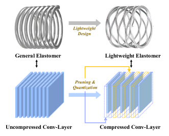
Figure 1: The analogy between the optimization in ED and MC.

In ED, the need to reduce weight and space for engineering applications has sparked two innovative ideas for elastomer optimization. On the one hand, materials with low EM should be removed as far as possible within cost constraints and replaced by more efficient and stable materials with higher EM. On the other hand, special design can be used to save space and costs. The thickness and width of the material, or the wave number of the lightweight elastomer can be varied to meet the requirements of different loads. Similarly, on the one hand, the MC can use network pruning which only keeps those filters that are relatively important, and those who have small FP should be deleted within each layer. On the other hand, quantization converts expensive floating point operations into hardware-friendly low-bit operations. The quantization bitwidth of each layer can also be adjusted by designed parameters. Motivated by the consistency in these two fields, useful ideas can be borrowed from ED to MC.

III-B Physics Inspired Criterion for Ranking Filters Globally

As step 1 in Figure 2 (a) shows, Hooke’s law is expressed as the elasticity of an elastomer deformed by linear stretching or shortening within the elastic limit following a force:

$$\sigma=\varepsilon\cdot{EM},$$ (1)

where $\sigma$ indicates the force that stretches or shortens the elastomer, $\varepsilon$ denotes the deformation by stretching or shortening, and $EM$ is a constant factor called the elasticity modulus. If we consider each convolutional layer as an elastomer, we can liken the FP to the EM, and the magnitude of the learnable scale can be viewed as the deformation. Thus, the $i$-th filter’s importance distribution $I_{i}^{l(i)}$ of depends on the product of a learnable deformation scale and the FP:

$$I_{i}^{l(i)}=a_{l(i)}\cdot FP\left(\boldsymbol{\Theta_{i}^{l(i)}}\right),$$ (2)

where $l(i)$ is the layer index for the $i$-th filter, $a_{l(i)}$ is the learnable deformation scale, $\boldsymbol{\Theta_{i}^{l(i)}}$ represents the $i$-th filter and $FP\left(\boldsymbol{\Theta_{i}^{l(i)}}\right)$ is the FP of the $i$-th filter. Although Hooke’s law has given us much inspiration, it cannot be fully replicated. Thus, two issues we need to address are: (1) Hooke’s law articulates an individual concept, meaning that it can only cover the importance ranking of a filter in its layer, which requires us to extend it to the global level. (2) The deformation of the elastomer is hand-crafted rather than automatic, whereas we need to further explore end-to-end automatic compression. For the first issue, a relative shift variable $b_{l(i)}$ is further introduced to rank filters cross-layers globally as shown in step 2 in Figure 2 (a):

$$I_{i}^{l(i)}=a_{l(i)}\cdot FP\left(\boldsymbol{\Theta_{i}^{l(i)}}\right)+b_{l(i)}.$$ (3)

EM is an intrinsic property of the elastomer that does not vary with force. It reveals the need to find an information metric characterizing FP, also an intrinsic property of the filters which does not change with external conditions. It has been observed in HRank [7] that the rank generated by a filter is robust to the input images. Therefore, a small batch of input images can be used to accurately estimate the expectation of the feature map rank as illustrated in Figure 2 (b). We use $D$ to denote the input images, which are sampled from a distribution $P(D)$. The rank of feature maps is shown to be not only a valid information measure but also a stable representation across $P(D)$. The underlying principle is that feature mapping is an intermediate step that can reflect both filters’ attributes and input images. Even within the same layer, different filters and their feature maps play different roles in the network [18, 19]. In addition, they capture how the input images are transformed in each layer and, finally, to the predicted labels. We define the FP as:

$$FP\left(\boldsymbol{\Theta_{i}^{l(i)}}\right)=\mathrm{R}\left(\mathbf{o}_{i}^{l(i)}(D)\right),$$ (4)

where $\mathbf{o}_{i}^{l(i)}(D)$ is the feature map of the $i$-th filter in the $l(i)$-th layer. $R(\cdot)$ is the rank of feature map for input images $D$. When inputting the $d$-th image in samplied input images $D$, the singular value decomposition (SVD) of $\mathbf{o}_{i}^{l(i)}(D^{d})$ is:

$$\begin{aligned} &\mathbf{o}_{i}^{l(i)}(D^{d})=\sum_{j=1}^{\left({r_{i}^{l(i)}}\right)^{d}}\delta_{j}u_{j}v_{j}^{T}\\ &=\sum_{j=1}^{\left({(r^{\prime})_{i}^{l(i)}}\right)^{d}}\delta_{j}u_{j}v_{j}^{T}+\sum_{j={\left({(r^{\prime})_{i}^{l(i)}}\right)^{d}}+1}^{\left({r_{i}^{l(i)}}\right)^{d}}\delta_{j}u_{j}v_{j}^{T},\end{aligned}$$ (5)

where $\delta_{j}$, $u_{j}$ and $v_{j}$ are left singular vectors, the previous $j$ singular values and right singular vectors of $\mathbf{o}_{i}^{l(i)}(D^{d})$, respectively. It can be seen that the feature map with rank ${r_{i}^{l(i)}}$ can be decomposed into a low-rank feature map with rank ${(r^{\prime})_{i}^{l(i)}}$ and some additional information. Thus, the high-rank feature map contains more information than the low-rank feature map. The rank $\mathrm{R}\left(\mathbf{o}_{i}^{l(i)}(D)\right)$ can be a reliable measure of information richness and be calculated as:

$$\mathrm{R}\left(\mathbf{o}_{i}^{l(i)}(D)\right)=\frac{1}{\left|D\right|}\sum_{d}^{\left|D\right|}{\left({r_{i}^{l(i)}}\right)^{d}},$$ (6)

where $\left|D\right|$ is the number of input images.

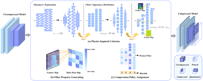
Figure 2: Overview of PIC-PQ framework. (a) Step 1 first shows a visual analogy between elastomers’ deformation in ED and filters’ importance distribution in MC. And it establishes a linear relationship that the filters’ importance distribution is linearly related to FP. In step 2, a relative shift variable is further introduced to rank filters cross-layers globally. (b) Then, the rank of the feature map from each filter is generated for obtaining the global importance ranking with the optimal $\boldsymbol{a-b}$ pairs searched before. (c) Finally, compression policy is assigned automatically.

The PIC above is based on the analogy between the ED and MC and plus a further design. In the following, we would like to derive this method from a mathematical theory perspective additionally. We want the compressed model after a series of optimization designs not only result in significant resource savings but also maintain lower accuracy drop compared to the original model. This is in line with the original intention of the MC, i.e., we want the difference in the loss function of the DNN before and after compression to be as small as possible. In mathematical problems, the Lipschitz continuity condition is often used to approximate the optimization problem of complex functions into a quadratic programming problem.

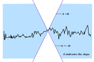
Figure 3: Lipshitz bound on the difference between the loss function of the baseline and the compressed model.

It can be seen that the inequality provides an upper bound on the variation amount of the function value in a neighborhood. In other words, it restricts the magnitude of the local variation not to exceed a certain constant. Figure 3 demonstrates the Lipschitz bound on the difference between the loss function of the baseline model and the compressed model. This mathematical formulation provides us not only with information about the envelope of the loss function difference but also new ideas for solving optimization problems with complex functions on the other. The Lipschitz continuity condition is defined as:

Theorem 1. For a function $f:U\subseteq\mathbb{R}^{m}\to\mathbb{R}^{n}$, if there exists a constant $\Omega\geq 0$ such that

$$\left\|f(y)-f(x)\right\|\leq\Omega\left\|y-x\right\|,\forall x,y\in U,$$ (7)

where $f$ satisfies the Lipschitz condition, and the constant $\Omega$ is called the Lipschitz constant for $f$.

So we can determine an upper bound on the difference in loss between the baseline and compressed model by assuming Lipschitz continuity. Therefore, we give the following optimization problem:

$$\begin{aligned} \min_{\mathbf{\mathcal{P}(m)}}\mathbb{L}\left(\boldsymbol{\Theta}\odot\mathbf{\mathcal{P}(m)}-\eta\sum_{j=1}^{\tau}\Delta\boldsymbol{w}^{(j)}\odot\mathbf{\mathcal{P}(m)}\right)-\mathbb{L}(\boldsymbol{\Theta}),\\ \text{ s.t. }C(\mathbf{\mathcal{P}(m)})\leq S_{budget},\end{aligned}$$ (8)

where $\mathbf{\mathcal{P}(m)}$ denotes the pruning-quantization joint learning strategy, where the binary variable $\mathbf{m}$ denotes the filter mask, and if the importance ranking of a filter is below a set threshold, $\mathbf{m}_{i}^{l(i)}=0$, otherwise $\mathbf{m}_{i}^{l(i)}=1$. The Hadamard product $\odot$ represents the multiplication of elements in corresponding positions, $\eta$ and $\tau$ denote the learning rate and the number of gradient steps respectively, and $\Delta\boldsymbol{w}^{(j)}$ denotes the gradient for the filter weights computed at step $j$. In terms of constraints, $C(\cdot)$ is the modeling function for computational complexity, and $S_{budget}$ is the required computational complexity constraint. Assuming that the loss function is $\Omega_{l}$-Lipschitz continuous for the $l$-th layer of the DNN, further, Eq. (8) can be transformed into a lagrangian form of minimizing its upper bound in terms of rank:

$$\min_{\mathbf{\mathcal{Q}(m)}}\sum_{i=1}^{I}\left(a_{l(i)}\cdot\mathrm{R}\left(\mathbf{o}_{i}^{l(i)}(D)\right)+b_{l(i)}\right)\mathbf{\mathcal{Q}(m_{i}^{l(i)})},$$ (9)

where $\mathbf{\mathcal{Q}(m)}=1-\mathbf{\mathcal{P}(m)}$, $a_{l(i)}=\Omega_{l(i)}$ and $b_{l(i)}=\eta\tau\Omega_{l(i)}^{2}-\lambda\hat{C}_{l(i)}$. $\hat{C}_{l(i)}$ denotes the computational complexity count at layer $l(i)$ of the baseline. That is, the process of globally cross-layers learning filter ranking can be seen as learning to estimate $\boldsymbol{a}$ and $\boldsymbol{b}$ and solving for the optimal solution to Eq. (9) to produce a better solution to the original objective. This is the same as Eq. (3) that we give in imitation of ED theory. the analogy between the ED and MC is a prerequisite for our formulation of the optimization objectives, and the subsequent mathematical derivation provides the theoretical support for Eq. (3). This forms a closed loop perfectly.

III-C The Derivation Process for the Transformation of Eq. (8)

Assuming that the loss function is $\Omega_{l}$-Lipschitz continuous for the $l$-th layer of DNN, Eq. (8) can be deflated to find an upper bound:

$$\begin{aligned} &\mathbb{L}\left(\boldsymbol{\Theta}\odot\mathbf{\mathcal{P}(m)}-\eta\sum_{j=1}^{\tau}\Delta\boldsymbol{w}^{(j)}\odot\mathbf{\mathcal{P}(m)}\right)-\mathbb{L}(\boldsymbol{\Theta})\\ \leq&\mathbb{L}(\boldsymbol{\Theta}\odot\mathbf{\mathcal{P}(m)})+\sum_{i=1}^{I}\Omega_{l(i)}\eta\left\|\sum_{j=1}^{\tau}\Delta\boldsymbol{w}_{i}^{(j)}\odot\mathbf{\mathcal{P}(m_{i}^{l(i)})}\right\|-\mathbb{L}(\boldsymbol{\Theta})\\ \leq&\sum_{i=1}^{I}\Omega_{l(i)}\left\|\boldsymbol{\Theta_{i}^{l(i)}}\right\|(1-\mathbf{\mathcal{P}(m_{i}^{l(i)})})+\sum_{i=1}^{I}\Omega_{l(i)}^{2}\eta\tau\odot\mathbf{\mathcal{P}(m_{i}^{l(i)})}\\ =&\sum_{i=1}^{I}\left(\Omega_{l(i)}\left\|\boldsymbol{\Theta_{i}^{l(i)}}\right\|-\Omega_{l(i)}^{2}\eta\tau\right)\mathbf{\mathcal{Q}(m_{i}^{l(i)})}+\Omega_{l(i)}^{2}\eta\tau,\end{aligned}$$ (10)

where $l(i)$ is the layer index of the $i$-th filter, $I$ indicates the total number of filters in the $l(i)$-th layer, $\mathbf{\mathcal{Q}(m)}=1-\mathbf{\mathcal{P}(m)}$, $||\cdot||$ denotes the arbitrary regularization tool.

The left-hand side of the constraint in Eq. (8) can be written in the following form:

$$\begin{aligned} &C({\mathbf{\mathcal{P}(m)}})=\sum_{i}^{I}c_{l(i)}\mathbf{\mathcal{P}(m_{i}^{l(i)})}\left\|\bigtriangleup\right\|_{0},c_{l(i)}\geq 0,\\ &\bigtriangleup=\left\{[\boldsymbol{\Theta}\odot\mathbf{\mathcal{P}(m)}]:[\boldsymbol{\Theta}_{j}\odot\mathbf{\mathcal{P}(m_{j})}]\forall j\in\Phi(l(i))\right\},\end{aligned}$$ (11)

where $\Phi(l(i))$ returns the set of filter indexes before layer $l(i)$ and $c_{l(i)}$ is a constant associated with the layer. Let $C_{l(i)}$ be the computational complexity count of layer $l(i)$ where filter $i$ resides, which depends linearly on the number of filters in the previous layer:

$$C_{l(i)}=c_{l(i)}\left\|\bigtriangleup\right\|_{0}.$$ (12)

Then Eq. (11) can be abbreviated as:

$$\begin{aligned} &C({\mathbf{\mathcal{P}(m)}})=C(\mathbf{1}-{\mathbf{\mathcal{Q}(m)}})\\ =&\sum_{i}^{I}C_{l(i)}{\mathbf{\mathcal{P}(m_{i}^{l(i)})}}=\sum_{i}^{I}C_{l(i)}\left(1-{\mathbf{\mathcal{Q}(m_{i}^{l(i)})}}\right).\end{aligned}$$ (13)

Let $\hat{C}_{l(i)}$ to denote the computational complexity count at layer $l(i)$ of the baseline network, and it follows that $C_{l(i)}\leq\hat{C}_{l(i)}$. Thus, there is the following form:

$$\begin{aligned} &C({\mathbf{\mathcal{P}(m)}})=C(\mathbf{1}-\mathbf{\mathcal{Q}})\\ &=\sum_{i}^{I}C_{l(i)}\left(1-\mathcal{Q}_{i}\right)\leq\sum_{i}^{I}\hat{C}_{l(i)}\left(1-\mathcal{Q}_{i}\right).\end{aligned}$$ (14)

Further, Eq. (8) can be transformed into a lagrangian form of minimizing its upper bound:

$$\begin{aligned} &\min_{\mathbf{\mathcal{Q}(m)}}\sum_{i=1}^{I}\left(\Omega_{l(i)}\left\|\boldsymbol{\Theta_{i}^{l(i)}}\right\|+\eta\tau\Omega_{l(i)}^{2}-\lambda\hat{C}_{l(i)}\right)\mathbf{\mathcal{Q}(m_{i}^{l(i)})}\\ &=\min_{\mathbf{\mathcal{Q}(m)}}\sum_{i=1}^{I}\left(a_{l(i)}\mathrm{R}\left(\mathbf{o}_{i}^{l(i)}(D)\right)+b_{l(i)}\right)\mathbf{\mathcal{Q}(m_{i}^{l(i)})}.\end{aligned}$$ (15)

III-D Quantization Bitwidth Automatically Assignment

After rank generating, PIC-PQ obtains the global importance ranking with the optimal $\boldsymbol{a-b}$ pairs learned. As Figure 2 (c) shows, finally, compression policy is assigned automatically to ensure meeting the constraints. As the filters’ importance knowledge is encoded in the $\boldsymbol{a-b}$ pairs, this process can be done efficiently without the need for training data. More importantly, there is no subjective human intervention or empirical parameter settings. Furthermore, in order to reduce the search space while ensuring an efficient hardware implementation, only different bitwidths are used between layers, but within layers, they are kept uniform.

Quantization bitwidth depends on the role of the quantized object in the overall model. For example, for over-parameterized filters, a lower quantization bitwidth can be chosen. At the same time, we also need to consider how to set the quantization bitwidth in terms of hardware resources. Based on the global importance ranking, we can determine the layer sparsity $S_{l}$ of $l$-th layer:

$$S_{l}=\frac{\left\|\mathbf{\Theta}_{l}\odot\mathbf{M}_{l}\right\|_{0}}{\left\|\mathbf{\Theta}_{l}\right\|_{0}},$$ (16)

where $\mathbf{\Theta}_{l}$ denotes the vector composed of filters in layer $l$, $\mathbf{M}_{l}$ denotes the sparse mask for layer $l$, which is composed of the filter mask $\mathbf{m}_{i}^{l(i)}$.

Then the quantization bitwidths of the weights and activation functions can be calculated according to:

$$n_{W_{l}}=\lceil N_{W_{l}}-\frac{p}{S_{l}}\rceil,n_{A_{l}}=\lceil N_{A_{l}}-\frac{p}{S_{l}}\rceil,$$ (17)

where $n_{W_{l}}$ and $N_{W_{l}}$ respectively correspond to the bitwidth for weight quantization and the available maximum bitwidth for $l$-th layer. Similarly, $n_{A_{l}}$ and $N_{A_{l}}$ do with quantization of the activation function. Penalty factor $p$ is a constant that can be adjusted according to the hardware.

For the $n_{W_{l}}$-bit weight and the $n_{A_{l}}$-bit activation output, the quantization function is:

$${W_{l}}^{q}=\frac{\operatorname{round}\left[\frac{\tanh\left({W_{l}}\right){2^{n_{W_{l}}-1}}}{\max\left(\left|{W_{l}}\right|\right)}\right]}{2^{n_{W_{l}}-1}}.$$ (18)

$${A_{l}}^{q}=\frac{\operatorname{round}\left[\operatorname{clamp}\left(A_{l},0,1\right)\bullet 2^{n_{A_{l}}}\right]}{2^{n_{A_{l}}}}.$$ (19)

We believe that the different input complexity of the layers of the network implies different precision requirements for the neurons. Neurons in shallower layers should be more sensitive to quantization [24]. Since the feature distributions overlap each other, a limited number of neurons will not be able to distinguish between samples and extract meaningful intermediate representations without the right precision. Once high-level features are explicitly obtained, later layers become more robust to quantization errors.

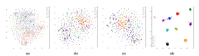
Figure 4: Two-dimensional feature representation of the inner layers of the ResNet56 network trained on CIFAR10. (a) Conv1 (first layer before Block 1) (b) Conv19 (last layer of Block 1) (c) Conv37 (last layer of Block 2) (d) Conv55 (last layer of Block 3).

To explore further, we trained a full-precision ResNet56 on CIFAR10. Drawing on the analytical approach from Chu et al. [24], 50 samples from each category are randomly selected and feed into the model at the end of training. T-SNE [25] is used to extract the feature representation of the inner layer and transform it into two-dimensional features. As shown in Figure 4, in the initial layer, there is significant confounding between the distribution of low-level semantic features of different categories. It is difficult to determine labels directly from the underlying features. Many fine neurons are required to distinguish between overlapping distributions. As the network propagates forward, features of the same class are gradually aggregated. As shown in Figure 4(d), the high-level semantic features are more robust, with clear boundaries between clusters of distributions of different categories at a deeper level.

Based on this observation, we tentatively corroborate the above opinion, and also consider that the shallow neurons should be more sensitive to quantization and the deeper layers more robust to quantization errors. Therefore, the available maximum bitwidth can be reduced as the layer deepens.

III-E Obtain the Compressed Model

Algorithm 1 Algorithm Description of PIC-PQ.

1:  Input: Randomly samplied images $D_{sample}$, baseline model $\boldsymbol{\Theta}$, constraint $S_{budget}$, random walk size $W$, total search iterations $E$, sample size $S$, mutation ratio $u$, population size $P$, fine-tuning iterations $\boldsymbol{\tau}$.

2:  Initialize $\boldsymbol{\Theta}$;

3:  Use $D_{sample}$ to generate rank R of feature maps;

4:  Initialize pool to a size of $P$;

5:  for $e=1$ to $E$ do

6:     a, b = Regularized EA ($W$, $S$, $u$, Pool);

7:     $\hat{\boldsymbol{\Theta}}^{\ast}$ = Fine-tuning ($\boldsymbol{\Theta}$, a, b, $\boldsymbol{\tau}$, $S_{budget}$, R);

8:     Score = $Acc_{val}(\hat{\boldsymbol{\Theta}}^{\ast})$;

9:     pool.replaceOldestWith(a, b, Score);

10:  end for

11:  Rank filters’ importance according to Eq. (3);

12:  Choose filters to prune, and assign bitwidth $n_{W_{l}},n_{A_{l}}$ for layers according to Eq. (17);

13:  Compress and fine-tune the model;

14:  Output: The best compressed model $\boldsymbol{\Theta^{\ast}}$ with highest $Acc_{val}(\boldsymbol{\Theta^{\ast}})$.

The filters’ importance distribution is updated by searching $\boldsymbol{a-b}$ pairs of layers. In the initial state, the distribution is unstressed and unmoving, meaning that $a_{l(i)}$ and $b_{l(i)}$ are 1 and 0 respectively. Learning $\boldsymbol{a-b}$ pairs under different constraints leads to different model compression effects. Meaning as in Algorithm 1, we use the regularized evolutionary algorithm (EA) proposed in [26] to learn $\boldsymbol{a}$ and $\boldsymbol{b}$.

Once learning $\boldsymbol{a}$ and $\boldsymbol{b}$, we fine-tune the pre-compressed architecture employing the $\boldsymbol{\tau}$ gradient step. Note that we use $\boldsymbol{\tau}$ to approximate $\boldsymbol{\hat{\tau}}$ (a fully fine-tuned step) and we empirically find that $\boldsymbol{\tau}=200$ works well. It is worth noting that, as in Figure 2 (a), the final global ranking of all filters is obtained when the optimal $\boldsymbol{a-b}$ pairs are learned. At this point, we can see that the filter with the highest global importance has the most information richness, and conversely, the filter with the lowest global importance has the least information richness. This confirms the feature interpretability.

IV Experiments

In this section, we conduct extensive experiments to demonstrate the effectiveness of our method. We first present the experiment setting in Section IV-A, and then we show the experiments of PIC-PQ on image classification benchmarks and compare them with state-of-the-art (SOTA) methods in Section IV-B.

IV-A Experiment Setting

IV-A1 Implementation Details

We evaluate the proposed method on the three benchmarks, CIFAR10, CIFAR100 [27] and ImageNet [28], and use standard training/test data splitting and data preprocessing on all datasets. For CIFAR10, we use the well-known ResNet56 [29] and VGG16 [30]. For CIFAR100, we use ResNet56 and MobilenetV2 [31]. And for ImageNet, we use ResNet18 and MobilenetV2. Of course, our method can be easily extended to other architectures.

All models are implemented based on PyTorch. For all benchmarks and architectures, we randomly sample 6 batches of images to estimate the average rank of each feature map. The mutation rate $u=10\%$ and the hyperparameters of the regularized evolutionary algorithm are set according to prior art [8]. We set the hyperparameter $\boldsymbol{\tau=200}$ for all experiments. When fine-tuning, the scheme follows [32] to use stochastic gradient descent [33] for all networks with a weight decay of 5e-4.

We use a single NVIDIA 2080Ti GPU for CIFAR10/100, and a single A100 GPU for ImageNet. For CIFAR10/100, we choose a batch size of 128 and an initial learning rate of 0.01 reduced by 5× at 30%, 60%, and 80% of the epochs respectively. For ImageNet, batch size is 256 and an initial learning rate is 0.001 who reduces by 10× at 30%, 60%, and 80% of the epochs respectively. We restrict selection space of available maximum bitwidth to $\left\{8,7,6,5,4,3,2\right\}$ bits and the weights and activations of a layer share the same bitwidth. The penalty factor $p$ for bitwidth assignment is uniformly 1/6. Based on the experience of Chakraborty et al. [34], we fix the first or/and last layers to full-precision in mixed precision quantization training. In addition, all the three residual connections in ResNet18 require larger bits than their corresponding regular branches.

Following the experience of [35, 10], the fine-tuning stage uses a distribution strategy. In the first step, we only fine-tunes a pruned model. In the second step, a network with mixed precision activation quantization and real-valued weights is fine-tuned. In the third step, the weights from the first step are inherited and the network is fine-tuned using mixed precision quantization for both weights and activations. The first step spends 400, 160, 60, 200, 100 and 100 epochs for the ResNet56 on CIFAR10, VGG16 on CIFAR10, ResNet56 on CIFAR100, MobilenetV2 on CIFAR100 networks, ResNet18 on ImageNet, MobilenetV2 on ImageNet respectively. The second step and third step both take 400 epochs for all networks on CIFAR10/100 and 100 epochs for all networks on ImageNet.

TABLE I: Comparison of compressing ResNet56 and VGG16 on CIFAR10.

ResNet56					VGG16
Method	P	Q	Top-1(%)↓	Comp. Ratio	Method	P	Q	Top-1(%)↓	Comp. Ratio
HRank [7]	$\surd$	$\times$	-0.26	1.41	Zhao et al. [36]	$\surd$	$\times$	0.78	1.64
PIC-P	$\surd$	$\times$	-0.93	1.43	GAL-0.05 [37]	$\surd$	$\times$	1.93	1.66
HRank [7]	$\surd$	$\times$	0.09	2.00	SSS [38]	$\surd$	$\times$	0.94	1.71
AMC [39]	$\surd$	$\times$	0.90	2.00	GAL-0.1 [37]	$\surd$	$\times$	3.23	1.82
Random Pruning [40]	$\surd$	$\times$	0.94	2.04	HRank [7]	$\surd$	$\times$	0.53	2.15
LRMF [41]	$\surd$	$\times$	0.34	2.11	PIC-P	$\surd$	$\times$	-0.45	2.17
FPGM [6]	$\surd$	$\times$	0.33	2.11	HRank [7]	$\surd$	$\times$	1.62	2.88
LFPC [42]	$\surd$	$\times$	0.35	2.12	PIC-P	$\surd$	$\times$	0.14	2.88
MaskSparsity [43]	$\surd$	$\times$	0.31	2.22	GM—3AS [44]	$\surd$	$\times$	0.90	4.12
PIC-P	$\surd$	$\times$	-0.03	2.13	l2—3AS [44]	$\surd$	$\times$	1.49	4.12
HRank [7]	$\surd$	$\times$	2.54	3.86	l1—3AS [44]	$\surd$	$\times$	1.31	4.12
PIC-P	$\surd$	$\times$	2.47	4.00	HRank [7]	$\surd$	$\times$	2.73	4.26
DNAS (Accurate) [45]	$\times$	$\surd$	-0.15	14.60	PIC-P	$\surd$	$\times$	0.69	4.26
DNAS (Efficient) [45]	$\times$	$\surd$	0.30	18.93	FSM [46]	$\surd$	$\times$	1.10	5.26
PIC-PQ	$\surd$	$\surd$	-0.63	33.50	PIC-PQ	$\surd$	$\surd$	0.11	43.06
PIC-P+FB	$\surd$	$\surd$	0.75	54.01	PIC-P+FB	$\surd$	$\surd$	1.14	71.92
PIC-PQ	$\surd$	$\surd$	0.10	54.96	PIC-PQ	$\surd$	$\surd$	0.75	76.43

IV-A2 Evaluation Metrics

In our experiments, classification performance is evaluated by overall accuracy, while FLOPs or BOPs compression ratio are employed to evaluate computational complexity. The BOPs metric has been used by DJPQ [17]. The BOPs for a convolution layer converting $C_{i}$ channels into $C_{o}$ channels is defined as:

$$\begin{aligned} BOPs=C_{i}C_{o}K^{2}H_{o}W_{o}B_{W}B_{A},\end{aligned}$$ (20)

where $K$ is the kernel size, $H_{o}$ and $W_{o}$ define the output spatial size, $B_{W}$ and $B_{A}$ denote weight and activation bitwidth of current layer. The BOPs compression ratio is defined as the ratio between the total BOPs of the uncompressed and compressed models.

Without loss of generality, we use the FLOPs compression ratio to measure only the pruning effect and use the BOP compression ratio to measure the overall effect from pruning and quantization. As seen from Eq.(20), BOPs count is a function of both number of channels remaining after pruning and quantization bitwidth, hence BOPs compression ratio is a suitable metric to measure a CNN’s overall compression.

In all tables that follow,“P”, “Q” indicate “pruning”, “quantization”, “Comp. ratio” indicates “BOPs compression ratio”, and “PIC-P+FB” indicates “PIC-P+Fixed bitwidth”.

IV-B Experiments and Comparisons

TABLE II: Compressing results of VGG16 on CIFAR10 under different compression ratios.

P	Q	Top-1(%)	Top-1(%)↓	Comp. Ratio
$\times$	$\times$	93.75±0.01	–	–
$\surd$	$\times$	96.06	-2.31	1.43
$\surd$	$\times$	96.44	-2.69	1.72
$\surd$	$\times$	94.20	-0.45	2.17
$\surd$	$\times$	93.61	0.14	2.88
$\surd$	$\times$	93.06	0.69	4.26
$\surd$	$\surd$	93.97	-0.22	31.58
$\surd$	$\surd$	93.70	0.05	37.64
$\surd$	$\surd$	93.64	0.11	43.06
$\surd$	$\surd$	93.00	0.75	76.43
$\surd$	$\surd$	92.00	1.75	101.71

IV-B1 Results on CIFAR10

The baselines for ResNet56 and VGG16 are 93.92% (±0.11%) and 93.75% (±0.10%) respectively, derived from multiple experiments. In Table I, for ResNet56, PIC-P outperforms comparison methods in terms of speed-up ratio and the accuracy drop when compressing 1.43× , 2.13× and 4×. PIC-PQ achieves a compression of 33.50× and an accuracy improvement of 0.63%, which is better than DNAS [45]. For VGG16, compared with SOTA methods at three different compression ratios, PIC-P is able to perform better in terms of accuracy drop while maintaining the same compression ratios.

More notably, we also evaluate PIC-P in combination with fixed bitwidth quantization as a two-stage approach and make sure that the pruning rate is very close. In comparison, PIC-PQ is able to maintain better accuracy at similar compression ratio when quantization bitwidth searching is performed, which demonstrates the effectiveness of our search-based approach.

Besides, we also give the compression results of VGG16 on CIFAR10 under different BOPs compression ratios.

We want to understand how our design affects the performance of the classification network. Specifically, we try PIC-P as well as PIC-PQ for VGG16 on CIFAR10 and configure five different compression ratios for PIC-P and PIC-PQ respectively, which users can use as a reference to choose according to their actual needs. The specific results are shown in Table II. We can see that with only pruning when compressing from 1.43× to 2.17×, the accuracy of each network improves, which indicates that the network does have a degree of redundancy, while we remove it in an interpretable way. In addition, joint learning method can compress better than pruning alone within a range of compression ratios.

TABLE III: Comparison of compressing ResNet18 and MobileNetV2 on ImageNet.

Method	P	Q	ResNet18			MobileNetV2
			Top-1(%)	Top-1(%)↓	Comp. Ratio	Top-1(%)	Top-1(%)↓	Comp. Ratio
Full-precision	$\times$	$\times$	69.75(±0.01)	–	–	71.81(±0.09)	–	–
EPruner [47]	$\surd$	$\times$	67.31	2.44	1.78	–	–	–
MFP [48]	$\surd$	$\times$	67.11	2.64	2.07	–	–	–
ManiDP [49]	$\surd$	$\times$	–	–	–	69.62	2.19	2.05
TWN[50]	$\times$	$\surd$	61.80	7.95	16.00	–	–	–
SR+DR [51]	$\times$	$\surd$	68.17	1.58	16.00	61.30	10.51	16.00
UNIQ [52]	$\times$	$\surd$	67.02	2.73	32.00	66.00	5.81	32.00
DFQ [53]	$\times$	$\surd$	65.80	3.95	64.00	70.43	1.38	16.00
RQ [54]	$\times$	$\surd$	61.52	8.23	64.00	68.02	3.79	28.44
DJPQ [17]	$\surd$	$\surd$	69.12	0.63	52.28	69.30	2.51	43.00
PIC-Q	$\times$	$\surd$	69.20	0.55	47.72	–	–	–
PIC-PQ	$\surd$	$\surd$	69.14	0.61	53.24	69.40	2.41	43.00

IV-B2 Results on ImageNet

Table III provides a comparison of PIC-PQ with other methods for compressing ResNet18 and MobileNetV2 on ImageNet. The results show a smooth trade-off achieved by PIC-PQ between accuracy and BOPs reduction. Compared with some fixed-bit quantization schemes, PIC-PQ achieves a significantly larger BOPs reduction. MobileNetV2 has been shown to be very sensitive to quantization [53]. Despite this, PIC-PQ is able to compress MobileNetV2 with a large BOPs compression ratio. PIC-PQ achieves a 43× BOPs reduction within 2.41% accuracy drop over DJPQ, where we set a similar global pruning rate.

TABLE IV: compressing results of MobilenetV2 on CIFAR100.

Method	P	Q	Top-1(%)	Top-1(%)↓	Comp. Ratio
Full-precision	$\times$	$\times$	75.12	–	–
PIC-P+FB	$\surd$	$\surd$	65.41	9.71	54.44
PIC-PQ	$\surd$	$\surd$	72.85	2.27	55.18

TABLE V: compressing results of ResNet56 on CIFAR100.

Method	P	Q	Top-1(%)	Top-1(%)↓	Comp. Ratio
Full-precision	$\times$	$\times$	70.66	–	–
PIC-P+FB	$\surd$	$\surd$	66.82	3.84	40.61
PIC-PQ	$\surd$	$\surd$	68.92	1.74	42.68

IV-B3 Results on CIFAR100

As we can see from Table IV, for MobilenetV2, PIC-PQ performs better than PIC-P+FB (Weight/Activation bitwidth (W/A) is 8/6) due to learning a better quantization strategy and preserving a higher quantization accuracy for some initial key layers of MobilenetV2. Similarly, we also compare PIC-PQ with PIC-P+FB on ResNet56 in Table V. PIC-PQ continues to have a lower accuracy loss than PIC-P+FB (W/A is 8/8) on ResNet56.

V Discussion

V-A Ablation Study: Validity Analysis of PIC.

TABLE VI: The effect of PIC for compressing ResNet56 on CIFAR10.

PIC	Comp. Ratio	Top-1(%)	Top-1(%)↓
$\surd$	1.43	94.01 →94.32	-0.31
$\times$	1.43	94.03 →93.36	0.67
$\surd$	2.13	94.03 →94.06	-0.03
$\times$	2.13	94.03 →92.02	2.01
$\surd$	4.00	94.03 →91.56	2.47
$\times$	3.33	94.03 →89.68	4.35

We investigate the effect of the PIC. We first turn off PIC-Q and then perform experiments with and without (default $\boldsymbol{a=1}$,$\boldsymbol{b=0}$) the PIC. The results are presented in Table VI, showing that in the absence of PIC for learning the optimal $\boldsymbol{a-b}$ pairs, the global ranking of the filters will be unguided and the accuracy decreases significantly at similar compression ratios compared to adopting PIC.

V-B Influence of the Fine-tuning Iterations in Searching the Optimal a-b Pairs

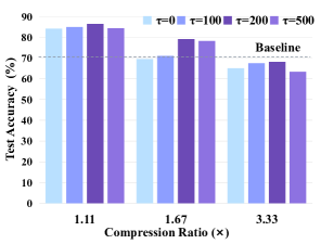
Figure 5: Influence of the $\boldsymbol{\tau}$.

The actual fine-tuning process is simulated in searching the optimal $\boldsymbol{a-b}$ pairs, where we further analyze the impact of the steps $\boldsymbol{\tau}$. We choose different $\boldsymbol{\tau}$ at three similar compression ratios, and once the optimal $\boldsymbol{a-b}$ pairs are learned, we compress ResNet56 on CIFAR100, where still only PIC-P is used. In the previous, we mention that $\boldsymbol{\tau}$ in searching the optimal $\boldsymbol{a-b}$ pairs approximates the fully fine-tuning steps $\boldsymbol{\hat{\tau}}$. We expect that the closer $\boldsymbol{\tau}$ to $\boldsymbol{\hat{\tau}}$, the better the optimization of the $\boldsymbol{a-b}$ pairs. In this experiment, 60 epochs are iterated, so that $\boldsymbol{\hat{\tau}}$ is fixed at 21120 gradient steps. As shown in Figure 5, $\boldsymbol{\tau}=200$ works well. The results are consistent with our intuition that continuing to increase $\boldsymbol{\tau}$ as we approach $\boldsymbol{\hat{\tau}}$ produces a decreasing effect.

V-C Is It Necessary to Search a-b Pairs in PIC Every Time

TABLE VII: Comparison of compressing VGG16 on CIFAR10 under “just-searching-once” and “searching-every-time”.

P	Q	searching-every-time		just-searching-once
		Top-1(%)	Comp. Ratio	Top-1(%)	Comp. Ratio
$\surd$	$\times$	96.04	1.43	96.06	1.43
$\surd$	$\times$	94.20	2.17	94.18	2.17
$\surd$	$\times$	91.34	4.55	91.32	4.55
$\surd$	$\surd$	93.95	31.60	93.97	31.58
$\surd$	$\surd$	93.64	43.06	93.58	44.28
$\surd$	$\surd$	91.38	119.18	92.00	101.71

In Table VII, “Searching-every-time” represents searching $\boldsymbol{a-b}$ pairs separately when compressing at different compression ratios. While “just-searching-once” means that after searching for the optimal solution of $\boldsymbol{a-b}$ pairs at a compression ratio to get the global ranking of the filters, you only need to use the obtained ranking information at other compression ratios. Here PIC-P and PIC-PQ use the prior knowledge searched at compression ratios of 1.43× and 31.58× respectively. Through Table VII, we find that both routes produce similar accuracy.

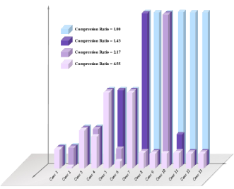
Figure 6: Comparison of the filter number remaining in each layer of VGG16 under just searching once.

In practice, our method relies on the assumption that the best-performing narrow network is a subset of the best-performing wide network. There are many model compression methods that achieve a given compression ratio by manually or automatically change the filter number in different layers, which means that there may be: compared to the best-performing large network, the best performing small network has a larger number of filters in some layers, but a smaller number of filters in some other layers. However, in our method, for a given network, it is only necessary to search and learn once, and this can be used to obtain compressed networks with different compression ratios. This assumption not only simplifies the tedious process of learning filter ranking, but also allows the user to have multiple choices of compression ratios under “just-searching-once”, which improves the efficiency of model compression.

Figure 6 plots a comparison of the filter number remaining in each layer of the VGG network under “just-searching-once”. From the Figure 6, we can not only see that our actual compression results satisfy the above subset of assumptions, but also confirm an opinion that the top layer is more stable and more inclined to be compressed than the lower layer.

VI Conclusion

In this paper, we propose a novel physics inspired criterion for pruning-quantization joint learning (PIC-PQ), where we make the first attempt to draw an analogy between ED and MC. A physics inspired criterion for ranking filters’ importance globally is explored from the analogy. We are well in line with the feature interpretability. Specifically, learnable deformation scale and FP in PIC are derived from Hooke’s law in ED. Besides, we further extend PIC with a relative shift variable to rank filters globally. An objective function is also put forward additionally from a mathematical theory perspective to demonstrate the viability of PIC. To ensure feasibility and flexibility, available maximum bitwidth and penalty factor are introduced in quantization bitwidth assignment. Experiments on benchmarks show that PIC-PQ is able to achieve a good trade-off between accuracy and BOPs reduction.

References

- [1] S. Ren, K. He, R. Girshick, and J. Sun, “Faster r-cnn: Towards real-time object detection with region proposal networks,” IEEE Trans. Pattern Anal. Mach. Intell., vol. 39, no. 6, pp. 1137–1149, 2017.
- [2] S. Li, W. Song, L. Fang, Y. Chen, P. Ghamisi, and J. A. Benediktsson, “Deep learning for hyperspectral image classification: An overview,” IEEE Geosci. Remote Sens., vol. 57, no. 9, pp. 6690–6709, 2019.
- [3] R. Girdhar, D. Tran, L. Torresani, and D. Ramanan, “Distinit: Learning video representations without a single labeled video,” in Proc. IEEE Int. Conf. Comput. Vis. (ICCV), 2019, pp. 852–861.
- [4] J. Cao, H. Cholakkal, R. M. Anwer, F. S. Khan, and L. Shao, “D2det: Towards high quality object detection and instance segmentation,” in IEEE Conf. Comput. Vis. Pattern Recog. (CVPR), 2020, pp. 11 482–11 491.
- [5] X. Ding, G. Ding, Y. Guo, and J. Han, “Centripetal sgd for pruning very deep convolutional networks with complicated structure,” in IEEE Conf. Comput. Vis. Pattern Recog. (CVPR), 2019, pp. 4943–4953.
- [6] Y. He, P. Liu, Z. Wang, Z. Hu, and Y. Yang, “Filter pruning via geometric median for deep convolutional neural networks acceleration,” in IEEE Conf. Comput. Vis. Pattern Recog. (CVPR), 2019, pp. 4340–4349.
- [7] M. Lin, R. Ji, Y. Wang, Y. Zhang, B. Zhang, Y. Tian, and L. Shao, “Hrank: Filter pruning using high-rank feature map,” in IEEE Conf. Comput. Vis. Pattern Recog. (CVPR), 2020, pp. 1529–1538.
- [8] T.-W. Chin, R. Ding, C. Zhang, and D. Marculescu, “Towards efficient model compression via learned global ranking,” in IEEE Conf. Comput. Vis. Pattern Recog. (CVPR), 2020, pp. 1518–1528.
- [9] Q. Zhou, S. Guo, Z. Qu, J. Guo, Z. Xu, J. Zhang, T. Guo, B. Luo, and J. Zhou, “Octo:INT8 training with loss-aware compensation and backward quantization for tiny on-device learning,” in Proc. USENIX Ann. Tech. Conf. (USENIX ATC 21), 2021, pp. 177–191.
- [10] Z. Liu, Z. Shen, M. Savvides, and K.-T. Cheng, “Reactnet: Towards precise binary neural network with generalized activation functions,” in Proc. Eur. Conf. Comput. Vis. (ECCV). Springer, 2020, pp. 143–159.
- [11] Z. Wang, H. Xiao, J. Lu, and J. Zhou, “Generalizable mixed-precision quantization via attribution rank preservation,” in Proc. IEEE Int. Conf. Comput. Vis. (ICCV), 2021, pp. 5291–5300.
- [12] S. Han, H. Mao, and W. J. Dally, “Deep compression: Compressing deep neural networks with pruning, trained quantization and huffman coding,” arXiv preprint arXiv:1510.00149, 2015.
- [13] C. Louizos, K. Ullrich, and M. Welling, “Bayesian compression for deep learning,” in Proc. Adv. Neural Inf. Process. Syst. (NIPS), 2017, p. 30.
- [14] S. Ye, T. Zhang, K. Zhang, J. Li, J. Xie, Y. Liang, S. Liu, X. Lin, and Y. Wang, “A unified framework of dnn weight pruning and weight clustering/quantization using admm,” arXiv preprint arXiv:1811.01907, 2018.
- [15] F. Tung and G. Mori, “Clip-q: Deep network compression learning by in-parallel pruning-quantization,” in IEEE Conf. Comput. Vis. Pattern Recog. (CVPR), 2018, pp. 7873–7882.
- [16] H. Yang, S. Gui, Y. Zhu, and J. Liu, “Automatic neural network compression by sparsity-quantization joint learning: A constrained optimization-based approach,” in IEEE Conf. Comput. Vis. Pattern Recog. (CVPR), 2020, pp. 2178–2188.
- [17] Y. Wang, Y. Lu, and T. Blankevoort, “Differentiable joint pruning and quantization for hardware efficiency,” in Proc. IEEE Int. Conf. Comput. Vis. (ICCV). Springer, 2020, pp. 259–277.
- [18] Y. Li, S. Lin, B. Zhang, J. Liu, D. Doermann, Y. Wu, F. Huang, and R. Ji, “Exploiting kernel sparsity and entropy for interpretable cnn compression,” in IEEE Conf. Comput. Vis. Pattern Recog. (CVPR), 2019, pp. 2800–2809.
- [19] Y. Zhang, M. Lin, C.-W. Lin, J. Chen, Y. Wu, Y. Tian, and R. Ji, “Carrying out cnn channel pruning in a white box,” IEEE Trans. Neural Netw. Learn. Syst., pp. 1–10, 2022.
- [20] T. Wang, K. Wang, H. Cai, J. Lin, Z. Liu, H. Wang, Y. Lin, and S. Han, “Apq: Joint search for network architecture, pruning and quantization policy,” in IEEE Conf. Comput. Vis. Pattern Recog. (CVPR), 2020, pp. 2078–2087.
- [21] X. He, Z. Mo, P. Wang, Y. Liu, M. Yang, and J. Cheng, “Ode-inspired network design for single image super-resolution,” in IEEE Conf. Comput. Vis. Pattern Recog. (CVPR), 2019, pp. 1732–1741.
- [22] M. Zhang, Q. Wu, J. Zhang, X. Gao, J. Guo, and D. Tao, “Fluid micelle network for image super-resolution reconstruction,” IEEE Trans. Cybern., vol. 53, no. 1, pp. 578–591, 2022.
- [23] M. Zhang, Q. Wu, J. Guo, Y. Li, and X. Gao, “Heat transfer-inspired network for image super-resolution reconstruction,” IEEE Trans. Neural Netw. Learn. Syst., pp. 1–11, 2022.
- [24] T. Chu, Q. Luo, J. Yang, and X. Huang, “Mixed-precision quantized neural networks with progressively decreasing bitwidth,” Pattern Recognit., vol. 111, p. 107647, 2021.
- [25] L. Van der Maaten and G. Hinton, “Visualizing data using t-sne.” J. Mach. Learn. Res., vol. 9, no. 11, 2008.
- [26] E. Real, A. Aggarwal, Y. Huang, and Q. V. Le, “Regularized evolution for image classifier architecture search,” in Proc. AAAI Conf. Artif. Intell. (AAAI), vol. 33, no. 01, 2019, pp. 4780–4789.
- [27] A. Krizhevsky, G. Hinton et al., “Learning multiple layers of features from tiny images,” Handbook of Systemic Autoimmune Diseases, 2009.
- [28] J. Deng, W. Dong, R. Socher, L.-J. Li, K. Li, and L. Fei-Fei, “Imagenet: A large-scale hierarchical image database,” in IEEE Conf. Comput. Vis. Pattern Recog. (CVPR). IEEE, 2009, pp. 248–255.
- [29] K. He, X. Zhang, S. Ren, and J. Sun, “Deep residual learning for image recognition,” in IEEE Conf. Comput. Vis. Pattern Recog. (CVPR), 2016, pp. 770–778.
- [30] K. Simonyan and A. Zisserman, “Very deep convolutional networks for large-scale image recognition,” arXiv preprint arXiv:1409.1556, 2014.
- [31] M. Sandler, A. Howard, M. Zhu, A. Zhmoginov, and L.-C. Chen, “Mobilenetv2: Inverted residuals and linear bottlenecks,” in IEEE Conf. Comput. Vis. Pattern Recog. (CVPR), 2018, pp. 4510–4520.
- [32] Y. He, G. Kang, X. Dong, Y. Fu, and Y. Yang, “Soft filter pruning for accelerating deep convolutional neural networks,” arXiv preprint arXiv:1808.06866, 2018.
- [33] Y. E. Nesterov, “A method for solving the convex programming problem with convergence rate o (1/k^ 2),” in Dokl. akad. nauk Sssr, vol. 269, 1983, pp. 543–547.
- [34] I. Chakraborty, D. Roy, I. Garg, A. Ankit, and K. Roy, “Constructing energy-efficient mixed-precision neural networks through principal component analysis for edge intelligence,” Nat. Mach. Intell., vol. 2, no. 1, pp. 43–55, 2020.
- [35] B. Martinez, J. Yang, A. Bulat, and G. Tzimiropoulos, “Training binary neural networks with real-to-binary convolutions,” arXiv preprint arXiv:2003.11535, 2020.
- [36] C. Zhao, B. Ni, J. Zhang, Q. Zhao, W. Zhang, and Q. Tian, “Variational convolutional neural network pruning,” in IEEE Conf. Comput. Vis. Pattern Recog. (CVPR), 2019, pp. 2780–2789.
- [37] S. Lin, R. Ji, C. Yan, B. Zhang, L. Cao, Q. Ye, F. Huang, and D. Doermann, “Towards optimal structured cnn pruning via generative adversarial learning,” in IEEE Conf. Comput. Vis. Pattern Recog. (CVPR), 2019, pp. 2790–2799.
- [38] Z. Huang and N. Wang, “Data-driven sparse structure selection for deep neural networks,” in Proc. Eur. Conf. Comput. Vis. (ECCV), 2018, pp. 304–320.
- [39] Y. He, J. Lin, Z. Liu, H. Wang, L.-J. Li, and S. Han, “Amc: Automl for model compression and acceleration on mobile devices,” in Proc. Eur. Conf. Comput. Vis. (ECCV), 2018, pp. 784–800.
- [40] Y. Li, K. Adamczewski, W. Li, S. Gu, R. Timofte, and L. Van Gool, “Revisiting random channel pruning for neural network compression,” in IEEE Conf. Comput. Vis. Pattern Recog. (CVPR), 2022, pp. 191–201.
- [41] X. Zhang, W. Xie, Y. Li, J. Lei, and Q. Du, “Filter pruning via learned representation median in the frequency domain,” IEEE Trans. Cybern., vol. 53, no. 5, pp. 3165–3175, 2023.
- [42] Y. He, Y. Ding, P. Liu, L. Zhu, H. Zhang, and Y. Yang, “Learning filter pruning criteria for deep convolutional neural networks acceleration,” in IEEE Conf. Comput. Vis. Pattern Recog. (CVPR), 2020, pp. 2009–2018.
- [43] N.-F. Jiang, X. Zhao, C.-Y. Zhao, Y.-Q. An, M. Tang, and J.-Q. Wang, “Pruning-aware sparse regularization for network pruning,” Mach. Intell. Res., vol. 20, no. 1, pp. 109–120, 2023.
- [44] D. Wang, S. Zhang, Z. Di, X. Lin, W. Zhou, and F. Wu, “A novel architecture slimming method for network pruning and knowledge distillation,” arXiv preprint arXiv:2202.10461, 2022.
- [45] B. Wu, Y. Wang, P. Zhang, Y. Tian, P. Vajda, and K. Keutzer, “Mixed precision quantization of convnets via differentiable neural architecture search,” arXiv preprint arXiv:1812.00090, 2018.
- [46] Y. Duan, Y. Zhou, P. He, Q. Liu, S. Duan, and X. Hu, “Network pruning via feature shift minimization,” in Proc. Asian Conf. Comput. Vis. (ACCV), 2022, pp. 4044–4060.
- [47] M. Lin, R. Ji, S. Li, Y. Wang, Y. Wu, F. Huang, and Q. Ye, “Network pruning using adaptive exemplar filters,” IEEE Trans. Neural Netw. Learn. Syst., vol. 33, no. 12, pp. 7357–7366, 2021.
- [48] Y. He, P. Liu, L. Zhu, and Y. Yang, “Filter pruning by switching to neighboring cnns with good attributes,” IEEE Trans. Neural Netw. Learn. Syst., pp. 1–13, 2022.
- [49] Y. Tang, Y. Wang, Y. Xu, Y. Deng, C. Xu, D. Tao, and C. Xu, “Manifold regularized dynamic network pruning,” in IEEE Conf. Comput. Vis. Pattern Recog. (CVPR), 2021, pp. 5018–5028.
- [50] B. Liu, F. Li, X. Wang, B. Zhang, and J. Yan, “Ternary weight networks,” in Proc. IEEE Int. Conf. Acoust. Speech Signal Process. (ICASSP). IEEE, 2023, pp. 1–5.
- [51] P. Gysel, J. Pimentel, M. Motamedi, and S. Ghiasi, “Ristretto: A framework for empirical study of resource-efficient inference in convolutional neural networks,” IEEE Trans. Neural Netw. Learn. Syst., pp. 5784–5789, 2018.
- [52] C. Baskin, N. Liss, E. Schwartz, E. Zheltonozhskii, R. Giryes, A. M. Bronstein, and A. Mendelson, “UNIQ: uniform noise injection for the quantization of neural networks,” ACM Trans. Comput. Syst., vol. 37, no. 1-4, pp. 1–15, nov 2019. [Online]. Available: https://doi.org/10.1145%2F3444943
- [53] M. Nagel, M. v. Baalen, T. Blankevoort, and M. Welling, “Data-free quantization through weight equalization and bias correction,” in Proc. IEEE Int. Conf. Comput. Vis. (ICCV), 2019, p. 1325–1334.
- [54] C. Louizos, M. Reisser, T. Blankevoort, E. Gavves, and M. Welling, “Relaxed quantization for discretized neural networks,” in Proc. Int. Conf. Learn. Represent. (ICLR), 2019.