HLRS2023

Modeling of Coupled Turbulent Channel-Porous Media Flow through a Deep Autoencoder-Echo State Network Framework

Abstract

In this study, we propose a novel approach, namely the combined Convolutional Deep Autoencoder–Echo State Network (CDAE-ESN) model, for the analysis and forecasting of dynamics and low-order statistics in coupled turbulent channel-porous media flows. Such systems find wide applications in industrial settings, including transpiration cooling and smart interface engineering. However, the complex geometry of coupled flow systems presents additional challenges for purely data-driven models. Our results demonstrate that the integration of deep autoencoder and echo state network techniques enables effective modeling and prediction of dominant flow behaviors, particularly within the porous domain exhibiting laminar regimes. To enhance the model’s applicability across a broader range of data domains, we further employ fine-tuning on a dataset encompassing varying porosities. The achieved average statistics exhibit a reasonable agreement, underscoring the efficacy of our proposed approach.

1 Introduction

Turbulent flow over permeable interfaces is ubiquitous in nature and engineering applications, from sediment transport to the transpiration cooling in gas turbines. Porous media are generally featured with complex topology in space (Chu et al, 2018b). A wide range of properties has been identified to have a significant effect on the mass and momentum transport across the porous medium-free flow interface. However, understanding and optimizing macro/micro-scale characteristics of porous media remains a challenge. This is due to both the difficulty of experimental measurements at the pore scale Terzis et al (2019) as well as the high costs of numerical simulations to resolve the full spectrum of scales.

Early studies of turbulent flows over permeable beds have addressed the effect of varying permeability on surface flows. The turbulent surface flow is similar to that of a canonical boundary layer when the interfacial permeability is low, as the near-wall structures are less disrupted. However, as the permeability increases, large-scale vortical structures emerge in the surface flow. This is attributed to Kelvin-Helmholtz (KH) type instabilities from inflection points of the mean velocity profile. More recently, the application of porous media for drag reduction inspired a series of in-depth studies on anisotropic permeability.

Direct Numerical Simulation (DNS) exhibits an edge of observing and analyzing turbulent physics in a confined small space, not only for the canonical cases as channel flows and pipe flows Chu et al (2016b); Pandey et al (2017b). Suga et al. Suga et al (2020) investigated the influence of the anisotropic permeability tensor of porous media at a higher permeable regime. It was found that streamwise and spanwise permeabilities enhance turbulence whilst vertical permeability itself does not. In particular, the enhancement of turbulence is remarkable over porous walls with streamwise permeability, as it allows the development of streamwise large-scale perturbations induced by the Kelvin–Helmholtz instability. However, DNS is still an expensive solution when one extend it for the parametric study often desired in the industrial context. It is still common to use analytical models or advanced turbulence models for this purpose which provide a reasonable accuracy in established applications. However, these models can diverge and model calibration is a time-consuming process.

Machine learning (ML) is on surge where it has successfully tackled many complex tasks ranging from self-driving cars, drug discovery, weather prediction, and more recently state-of-the-art large language models such as GPT for natural language processing. Machine learning has been democratized heavily in the last decade and some of the reasons include vast availability of open-source libraries, active community, huge volume of incoming data from physical as well as numerical experiments and an ease in access to high-performance computing resources via cloud. In recent years, ML has shown potential in the modelling of various fluid flow use-cases (Pandey et al, 2022; Fang et al, 2019; Chu et al, 2018a; Pandey et al, 2020b). Typically, big data ML problems rely upon some kind of feature extraction process e.g. conventional feature selection process, long-standing proper orthogonal decomposition (POD), relatively new dynamic mode decomposition (DMD) Kutz et al (2016) or ML based methods (Storcheus et al, 2015). Feature extractor transform the input raw data into information preserving feature vector with a primary goal of reducing the dimensionality of the data. Several attempts have been made in the past few years to combine POD or DMD with machine learning (Pandey and Schumacher, 2020). However, these methods have certain limitation especially when the flow advances in the turbulent flow regimes. Therefore, an end-to-end machine learning system is being suggested where POD and DMD is replaced by a non-linear DNN (Pandey and Schumacher, 2020; Nakamura et al, 2021). A common architecture is deep convolution autoencoder (DAE) to extract the features for further processing and decision making. Turbulent flow problems often involve tempo-spatial data, therefore, extracted features could be used to train a downstream network to build a data-driven dynamic model. A common choice is a recurrent neural network (RNN) which preserves the sequential relationship in a time series. A combination of such approaches has shown exemplary results in terms of data compression and modeling.

In this work, we make an attempt to model complex flow behaviors in a porous medium with the help of a data-driven approach. The flow is in a turbulent regime and due to the presence of porosity, geometry is resolved to a finer scale. This setup makes the end-to-end ML task challenging and equally interesting. The goal is to combine the deep learning based feature extraction step followed by a recurrent neural network to model temporal evolution. Echo state network was chosen as the RNN due to its proven efficiency in modeling multi-dimensional tempo-spatial data. The trained models are restricted to the domain of training and work poorly beyond the trained data domain which could be a specific parameter such as Reynolds number. A commonly used strategy called transfer learning is used, where the objective is to transfer the gained knowledge from the training of source task to related target task with a limited dataset Zhuang et al (2020). Fine tuning, which can be considered as a part of transfer learning, is one methodology where an already trained and optimized model tuned with another similar set of data for a similar task. This could decrease the training time significantly in addition to neural architecture search and training data requirements. Fine-tuning can be performed on the entire network level where we allowed to retrain all the layers while initializing the parameters with the pretrained model. Alternatively, several layers can be freeze and retraining is allowed on only few layers. The former method is suitable when network size is very large and data is limited. While first approach could lead to the overfitting Yosinski et al (2014). Therefore, we also present the result from fine-tuning where trained model from a given data domain was transferred to a different data domain.

2 Synthetic data generation

In our DNS, the three-dimensional incompressible Navier$-$Stokes equations are solved in non-dimensional form,

$$\frac{\partial u_{j}}{\partial x_{j}}=0$$ (1)

$$\frac{\partial u_{i}}{\partial t}+\frac{\partial u_{i}u_{j}}{\partial x_{j}}=-\frac{\partial p}{\partial x_{i}}+\frac{1}{Re_{D}}\frac{\partial^{2}u_{j}}{\partial x_{i}\partial x_{j}}+\Pi\delta_{i1}$$ (2)

where $\Pi$ is a constant pressure gradient in the mean-flow direction. The governing equations are normalized using the half-width of the whole simulation domain $H$(figure 1) and the averaged bulk velocity $U_{b}$ of the channel region ($y/H=[0,1]$). Hereafter, the velocity components in the streamwise $x$, wall-normal $y$, and spanwise $z$ directions are denoted as $u$, $v$, and $w$, respectively. The domain size ($L_{x}/H\times L_{y}/H\times L_{z}/H$) is $10\times 2\times 0.8\pi$ in all cases. The lower half ($y/H=[-1,0]$) contains the porous media, and the upper half ($y/H=[0,1]$) is the free channel flow. The porous layer consists of 50 cylinder elements along the streamwise direction and 5 rows in the wall-normal direction, as illustrated in figure 1. The distance $D$ between two nearby cylinders is fixed at $D/H=0.2$. No-slip boundary conditions are applied to the cylinders, the upper wall, and the lower wall. Periodic boundary conditions are used in both streamwise and spanwise directions.

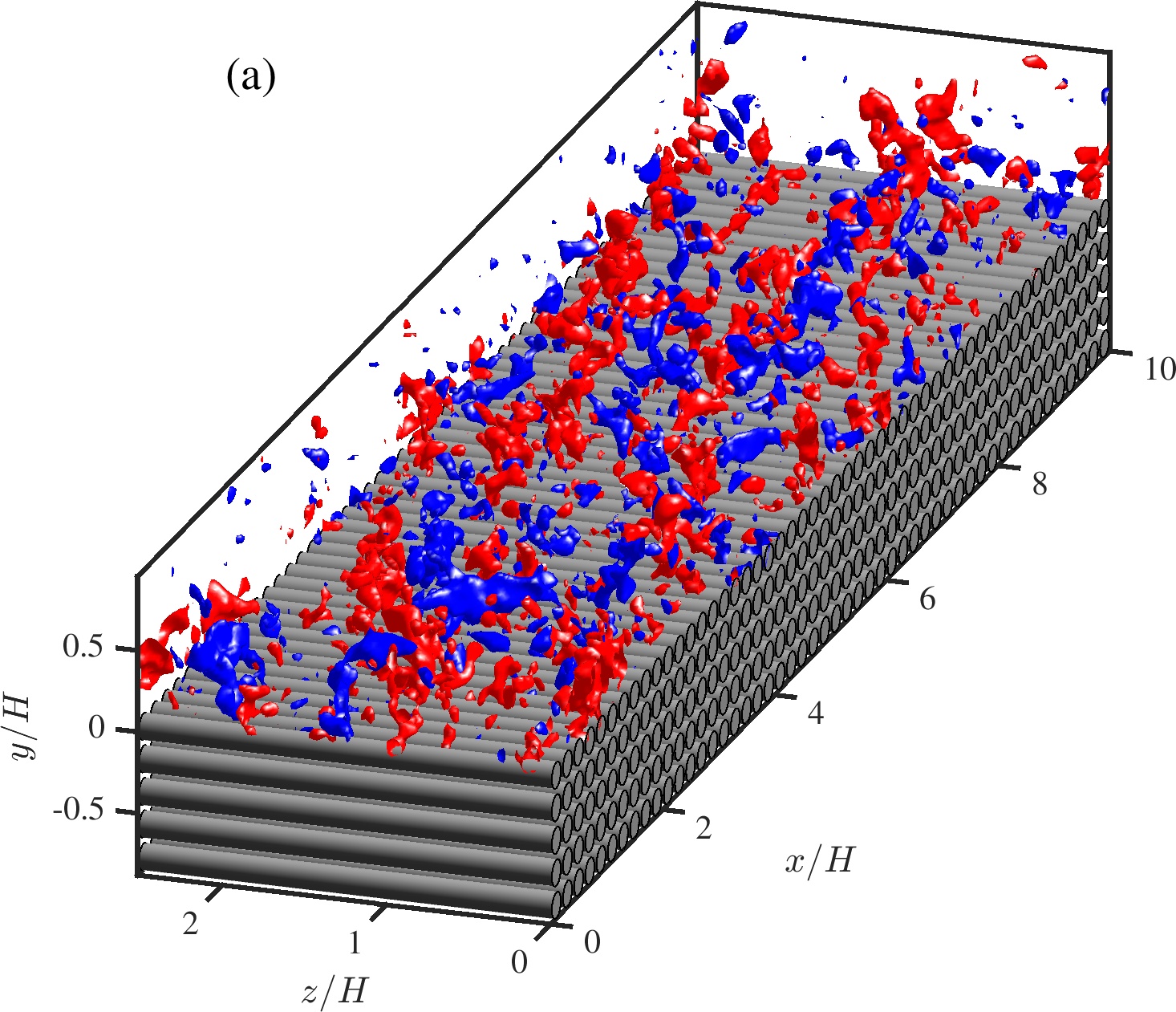
Figure 1: Configuration of the computational domain (C05), the permeability in three directions can be found in Table 1. The blue and red isosurfaces show the wall-normal fluctuation $v^{\prime}/u^{p}_{\tau}$ at level $-0.4$ and $0.4$, respectively.

The spectral/$hp$ element solver Nektar++ is used to solve equations (1, 2) (Cantwell et al, 2011; Chu et al, 2019, 2020; Pandey et al, 2020a; Chu et al, 2021b, a; Wang et al, 2021b, 2022). The geometry in the $x$-$y$ plane is discretized into quadrilateral elements with local refinement near the cylinders (see figure 1). Local element expansions are applied based on the modified Legendre basis (Karniadakis et al, 2005). We used flexible polynomial orders across the wall normal range in a continuous Galerkin projection. The polynomial order in the free flow region $y/H=[0.2,1]$ is $P=6$-$7$. The near wall region and the top two layers of cylinders $y/H=[-0.4,0.2]$ are enhanced with a higher order of $P=8$-$9$. A lower order of $P=5$ is selected in the deeper positions of the cylinder array ($y/H=[-1,-0.4]$). The spanwise direction is extended with a Fourier spectral method. The 2/3 rule is used to avoid aliasing errors. The time-stepping is performed with a second-order mixed implicit-explicit (IMEX) scheme. The time step is fixed at $\Delta T/(H/U_{b})=5\times 10^{-4}$.

Case	$\varphi$	$Re_{\tau}^{p}$	$Re_{\tau}^{s}$	$\sqrt{K_{xx}}^{p+}$,$\sqrt{K_{yy}}^{p+}$	$\sqrt{K_{zz}}^{p+}$	$C_{xx}^{{p+}},C_{yy}^{{p+}}$	$r_{c}^{{p+}}$	$C_{f}^{p}$	$C_{f}^{s}$
C05	0.5	336	180	4.55	8.86	0.37	42	0.0112	0.0084
C06	0.6	464	190	9.34	15.23	0.58	48	0.0149	0.0085

Table 1: Simulation parameters. The porosity of the porous medium region is $\varphi$. The friction Reynolds numbers are $Re_{\tau}^{p}$ and $Re_{\tau}^{s}$ for the porous and impermeable top walls respectively. $\sqrt{K_{\alpha\alpha}}^{p+}$ and $C_{\alpha\alpha}^{{p+}}$ are the diagonal components of the permeability tensor and Forchheimer coefficient, respectively, in the direction of $\alpha$ ($\alpha\in\{x,y,z\}$), which are normalized by wall units. $r_{c}^{{p+}}$ is the radius of the cylinders.

Four DNS cases are performed with varying porosity $\varphi=0.5$ and 0.6, which is defined as the ratio of the void volume to the total volume of the porous structure. The parameters of the simulated cases are listed in table 1, where the cases are named after their respective porosity. The superscripts $(\cdot)^{p}$ and $(\cdot)^{s}$ represent permeable wall and smooth wall side variables, respectively. Variables with superscript ⁺ are scaled by friction velocities $u_{\tau}$ of their respective side and viscosity $\nu$.

For an arbitrary variable $\phi$, we denote the time averaged value as $\overline{\cdot}$, i.e., $\overline{\phi}=1/T\int_{0}^{T}\phi\mathrm{d}t$, and spatial averaged value in $x$-$z$ plane as $\langle\cdot\rangle$, i.e., $\langle\phi\rangle=1/A_{f}\int_{A_{f}}\phi\mathrm{d}A$, $A_{f}$ being the fluid area. The instantaneous turbulent fluctuation is $\phi^{\prime}=\phi-\overline{\phi}$, and form-induced fluctuation is $\widetilde{\overline{\phi}}=\overline{\phi}-\langle\overline{\phi}\rangle$. For the permeable wall side, the total shear stress at the interface can be derived as:

$$\tau_{w}^{p}=\left(\mu\frac{\partial\langle\overline{u}\rangle}{\partial y}-\rho\langle\overline{u^{\prime}v^{\prime}}\rangle-\rho\langle{\overline{u}}\rangle\langle{\overline{v}}\rangle-\rho\langle{\tilde{\bar{u}}\tilde{\bar{v}}}\rangle\right)_{y=0}.$$ (3)

For the smooth wall side,

$$\tau_{w}^{s}=\left(\mu\frac{\partial\langle\overline{u}\rangle}{\partial y}\right)_{y=H},$$ (4)

The friction velocity can then be calculated from total shear stress at both walls $u_{\tau}=\sqrt{\tau_{w}/\rho}$. The friction coefficient is defined as $C_{f}=\tau_{w}/(\frac{1}{2}\rho U_{b}^{2})$, which is listed in table 1.

Note that the distance between cylinders is fixed, and the porosity is changed by varying the radius of the cylinders. The normalized cylinder radius is in the range $r_{c}^{p+}=r_{c}u_{\tau}^{p}/\nu=42$-$48$ for all the cases tested (see table 1), such that the effect of surface roughness is assumed to be at a similar level. For all the cases, the Reynolds number of the top wall boundary layer is set to be $Re_{\tau}^{s}=\delta^{s}u_{\tau}^{s}/\nu\approx 180$ ($\delta$ is the distance between the position of maximum streamwise velocity and the wall). In this manner, changes in the top wall boundary layer are minimized. On the top smooth wall side, the streamwise cell size ranges from $4.1\leq\Delta x^{s+}\leq 6.3$ and the spanwise cell size is below $\Delta z^{s+}=5.4$. On the porous media side, $\Delta z^{p+}$ is below 8.4, whereas $\Delta x^{p+}$ and $\Delta y^{p+}$ are enhanced by polynomial refinement of local mesh. The total number of grid points ranges from 88$\times 10^{6}$ (C05) to 595$\times 10^{6}$ (C08). Each cylinder in the porous domain is resolved with 80 to 120 grids along the perimeter. The spatial resolution of current work is close to those of previous DNS researches. For example, Shen et al (2020) conducted DNS of a turbulent flow over sediment beds using the immersed boundary method, where the diameter is discretized into 36-50 points. The mesh of Karra et al (2022) has 26 grid points along the diameter of each grain.

By performing parameter tests on porous media and fitting the Darcy-Forchheimer equation, the permeability tensor $K$ and Forchheimer coefficient $C$ may be obtained, and the details of the computation can be referred to Wang et al (2021a). The intensity profiles of $u^{\prime}$, $v^{\prime}$, and $w^{\prime}$ are shown in figure 1(b-d), respectively. The turbulent intensity grows with porosity for both the channel and the porous medium region. In the current study, we focus on the up and down-welling motions at the upper surface of the porous medium, which is represented by the fluctuation $v^{\prime}$.

3 Data-driven modelling

Data driven modelling (DDM) is an approach to harness the available data about a system and establish a connection between the system state variables (input, internal and output variables) without explicit knowledge of the physical behaviour Solomatine et al (2008). In this work, we have the synthetic data derived from the DNS while the end model should be based upon this data and should able to provide an model to predict temporal evoliution of a state variable. Figure 2 depicts our end-to-end 2-step ML framework. To have an extendable framework, we chose to first extract the features with the help of a deep encoder and feed the extracted features to a second level recurrent neural network (RNN). This architecture is inspired from our earlier work Pandey et al (2022).

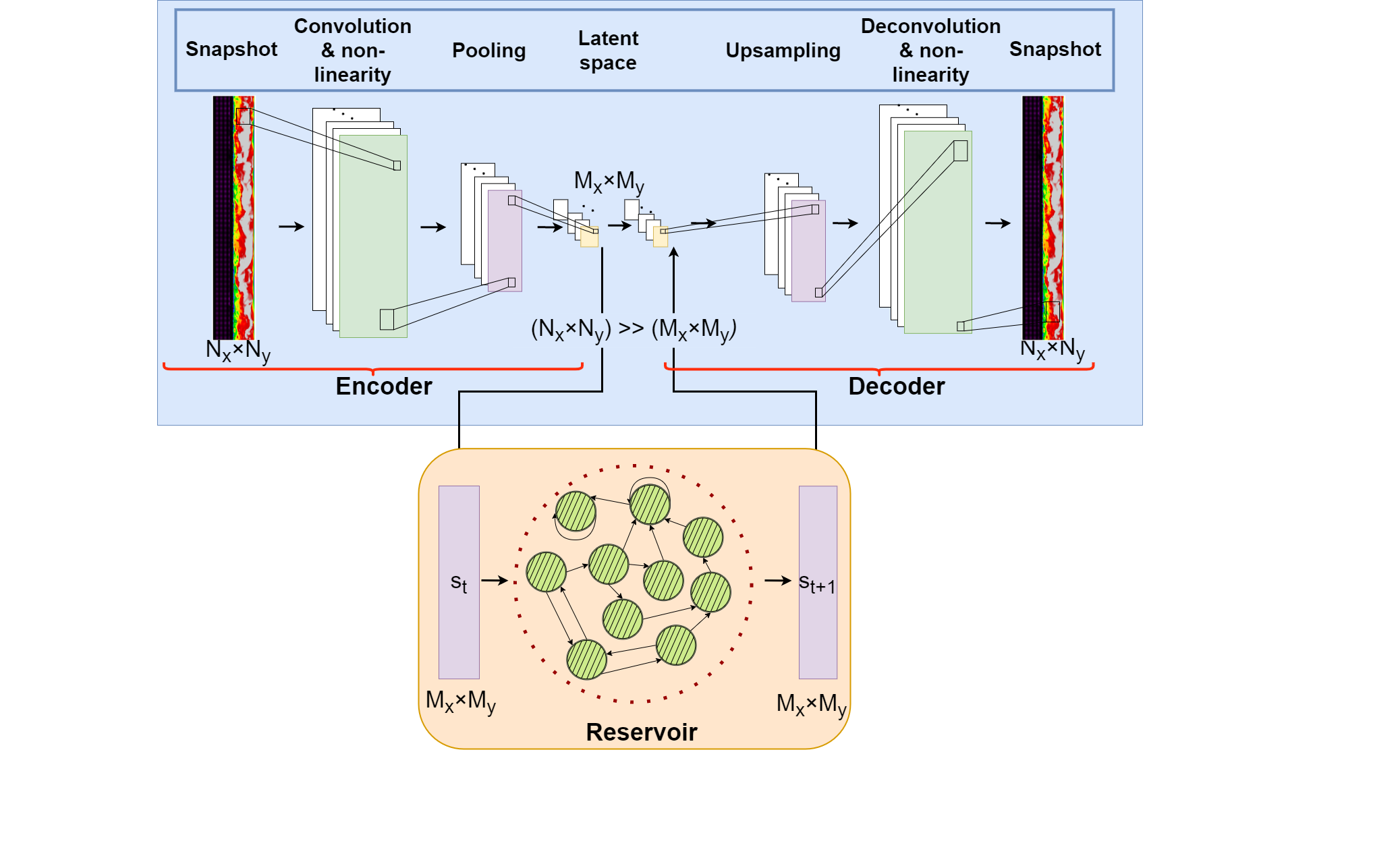
Figure 2: Two-step machine learning architecture for end-to-end ROM model for porous media. In the first step, DAE is trained as feature extractor cum decoder while the second step trains the extracted feature in autoregressive manner.

3.1 Feature extraction with autoencoder

The deep convolution autoencoder (DAE) is an implementation of an unsupervised machine learning paradigm, where the training of the model does not rely upon the labeled data. The objective of learning is to extract efficient representations or features in a low-dimension hyper-plane that can reproduce the data with minimal reconstruction error. That is to say, an autoencoder encodes input data $\bm{I}$ into $\bm{c}=\textnormal{encode}(\bm{I})$ with $\bm{c}\in\mathbb{R}^{l}$. And it decodes $\bm{c}$ back into $\hat{\bm{I}}=\textnormal{decode}(\bm{c})$ subsequently. The reconstruction error is calculated with $\hat{\bm{I}}-\bm{I}$. Here, 2-dimensional data were obtained from the DNS as described in Sec. 2. Thus autoencoder consists of several convolution layers resulting in a deep architecture. Each convolution layer in the network acts as a local feature extractor and shares the weights. The convolution layer is followed by a pooling layer, max pooling in this case, which reduces the dimension and focuses on the non-repeating key features. It gives a unique property of translation invariance to the network. At the end of the encoder network, there is a bottleneck layer that has the latent space or extracted features. These features are then passed to a decoder section which will attempt to recreate the original DNS data from the features. The training starts with random initialization of all the weights in the network and learns them as per the loss function via backpropagation.

3.2 Echo State Network (ESN)

ESN is closely related to reservoir computing (RC) and it shines out with sequential data where temporal relationship is present. In a typical ESN setup, input data is fed to a input layer which is connected to a big sparse reservoir which is finally connected to an output layer. ESN differs from typical RNN in terms of not requiring a back-propagation, therefore, it is inherently fast in training. More details can be found in our earlier work Pandey et al (2022). In this work, ESN acts as a downstream network which learns to predict the temporal evolution of the features obtained by the encoder section of DAE in an auto-regressive manner. The predicted values can be fed back to the decoder section of DAE to reproduce the feature of interest. Therefore, the during the deployment, we are only interested in the trained ESN and decoder while encoder can be thrown away.

4 Results and Discussion

4.1 Data driver flow model

As mentioned earlier, we first trained a DAE network to extract the feature in a lower-dimensions. For the same, input and output layer has the same dataset i.e. the snapshots from the DNS consist of $u$-velocity component with a dimension of $1501\times 109\times 1$. The neural network has multiple convolution layers combined with a max pooling layer while the decoder section has a convolution layer and a up-sampling layer, giving a converging-diverging shape. The features or latent modes are obtained at the end of the encoder section and it has a shape of $24\times 2\times 34$, thereby giving a dimensionality reduction of 99%. This could increase further on the expense of reconstruction loss. Table 2 illustrates the various layers and their shape. After fixing the DAE architecture, various hyperparameters were obtained by using Bayesian optimization. This particular approach is part of the AutoML paradigm He et al (2021), and it assists in achieving an optimized set of parameters in a relatively less number of iterations when compared to random or grid search. It is worth to mention that the data were scaled between 0-1 before the training.

Encoder			Decoder
Layer	Output size		Layer	Output size
Encoder input	$1501\times 109\times 1$		Decoder input	$24\times 2\times 34$
2D Conv-E1	$1501\times 109\times 256$		2D Conv-D1	$24\times 2\times 34$
Max Pool-E1	$751\times 55\times 256$		2D Upsamp-D1	$48\times 4\times 34$
2D Conv-E2	$751\times 55\times 256$		2D Conv-D2	$48\times 4\times 32$
Max Pool-E2	$376\times 28\times 256$		2D Upsamp-D2	$96\times 8\times 32$
2D Conv-E3	$376\times 28\times 128$		2D Conv-D3	$96\times 8\times 64$
Max Pool-E3	$188\times 14\times 128$		2D Upsamp-D3	$192\times 16\times 64$
2D Conv-E4	$188\times 14\times 64$		2D Conv-D4	$192\times 16\times 128$
Max Pool-E4	$94\times 7\times 64$		2D Upsamp-D4	$384\times 32\times 128$
2D Conv-E5	$94\times 7\times 32$		2D Conv-D5	$384\times 32\times 256$
Max Pool-E5	$47\times 4\times 32$		2D Upsamp-D5	$768\times 64\times 256$
2D Conv-E6	$47\times 4\times 34$		2D Conv-D6	$768\times 64\times 256$
Max Pool-E6	$24\times 2\times 34$		2D Upsamp-D6	$1536\times 128\times 256$
			Output with 2D Conv	$1536\times 128\times 1$
			Output with Cropping	$1501\times 109\times 1$

Table 2: DAE architecture used at first level for feature extraction. The table summarizes the encoder and decoder architectures (Conv = convolution, Max Pool = max pooling, Upsamp = upsampling). Symbol E2 denotes for example encoder hidden layer No. 2.

Once DAE is trained, we extract the features for the entire dataset using its encoder part. These encoded data which has 99% reduced dimension were further used to train the second level of RNN i.e. ESN. Unlike DAE, training an ESN is relatively straightforward and computationally cheaper because of straightforward design choices. The optimized network of ESN has 3726 reservoirs, 0.93 as spectral radius, 0.94 as leaking rate and 0.16 as reservoir density. For the best results, the look back history period is 4 timesteps i.e., model requires 4 timesteps data as an initialization then the system can predict auto-regressively. As a first step of validation, we visualize the low-dimensional features from the DAE along with the generated data from ESN on the blind validation set. We call the method generative because the model works auto-repressively once we provide the initialize data. Figure 3 shows such time-series for 2 of the modes out of 1632. It is impressive that model maintain a value of 0 without any minor fluctuations for $\phi_{1}$ while series fluctuates with the right phase and amplitude for $\phi_{10}$. Figure 4 further illustrates the probability density function (PDF) of these 2 modes for the DAE and ESN. It reaffirms the generating capability of ESN where it is able to match the overall distribution with the ground trouth.

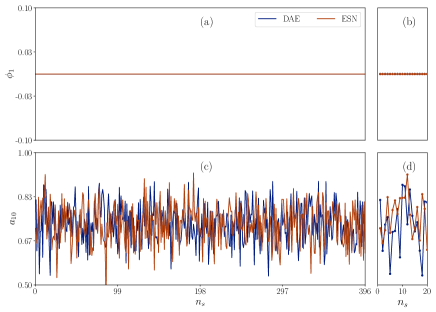
Figure 3: A comparison of extracted features from DAE which acts as ground truth for the training, and prediction from ESN for 2 of the modes.

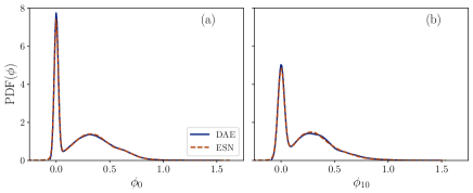
Figure 4: Comparison between DAE and ESN modes in terms of pdf for 2 of the modes

As a next step of validation is the comparison in high-dimensional space where flow physics need to be captured. Figure 5 displays contour plots of the original DNS data in panels (c) and (f), reconstructed data from the features space of the DAE in panels (b) and (e), and the decoded value from the prediction of ESN is shown in panels (a) and (d). One can observe a good qualitative agreement in terms of capturing the flow fields. Both regions i.e. main channel flow and porous flow can be predicted. Both DAE and ESN were trained from the DNS, and are not able to fully capture the strong turbulent field in the channel. While the flow in the porous media section is much better because it falls within the laminar region mostly. The obvious reason is the limited capability of DAE to capture the entire flow field because it discards 99% of input data and usage only 1% of the features, similar to conventional reduced-order modelling approach such as POD. The derived model with ESN shows an excellent result while matching field compared to its GT i.e. DAE. It suggests that the entire model can further be improved if a state-of-the-art feature extractor such as transformer model can be used instead of DAE. It is worth to mention DAE surpasses conventional as well as some advance feature extractors e.g., variational autoencoder for this use-case, which was observed in our experimentation. Often, average and fluctuations are critical values for the analysis in industrial applications. Therefore, we further validate the results with mean and fluctuations profile over the cross-section of the channel. Figure 6 shows these profiles and a mean velocity profile overlap with the DNS for both DAE and ESN. The fluctuation of velocity is slightly deviated in the main channel while they remain zero in the porous section due to dominating laminar flow. The distinction made by the model is also great where it can predict the interface where flow is transiting from laminar to turbulent.

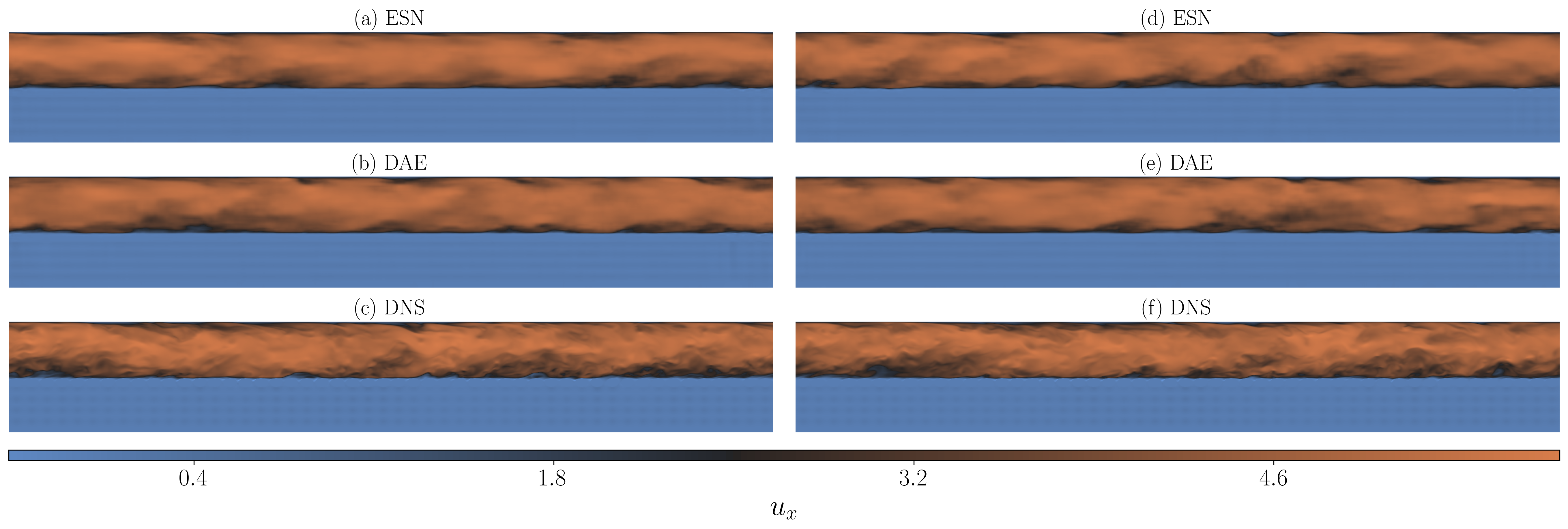
Figure 5: Contours of $u_{x}$ by (a,d) ESN (final end to end model), (b,e) DAE (feature extractor) and (c,f) DNS (GT) at 2 different timestamps.

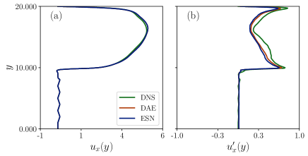
Figure 6: Comparison among ground truth (DNS), reduced order model (DAE) and temporal model for DAE modes using ESN. (a): Average fields (b) Fluctuations

4.2 Fine tuning

The trained model has shown a good agreement in terms of quantitative as well as qualitative characteristics of the flow. However, the trained model is limited to a given data domain that was used for the training which means that the model will not predict accurate results as we use different conditions. This is one of the biggest downsides of such a data-driven model. There are several approaches that one can use to increase the applicability of such a model to a wider data domain. In this work, we assess the fine-tuning which is widely used in the machine-learning community. Fine-tuning makes the use of existing trained model and tune it with the newer limited data. As mentioned earlier, DAE is a computationally expensive component of this workflow, therefore, we further assess DAE with the fine-tuning. We tested the DAE model with a different set of data. Here, we used case C06 which has a higher level of porosity compared therefore a higher Reynolds number as mentioned in Table 1.

Case Name	Description	Training time	Mean Square Error
DNS	Simulation results which acts as GT for case C06	-	-
DAE90	Model trained from scratch similar to case C05	O(103)	0.025
DAE91	Direct prediction using model from case C05 without any training	0	0.081
DAE92	Model from case C05 retrained with all data points for case C06	O(102)	0.030
DAE93	Model from case C05 retrained with 10% data points for case C06	O(101)	0.049

Table 3: Various cases considered for fine tuning.

Table 3 shows the cases used for the fine tuning study and corresponding results are shown in Figures 7 and 8. For the averaged streamwises velocity profile and its fluctuation, the reduced-order model shows comparable results as in its original validation, which proves the validity of the methodology of the fine-tuning.

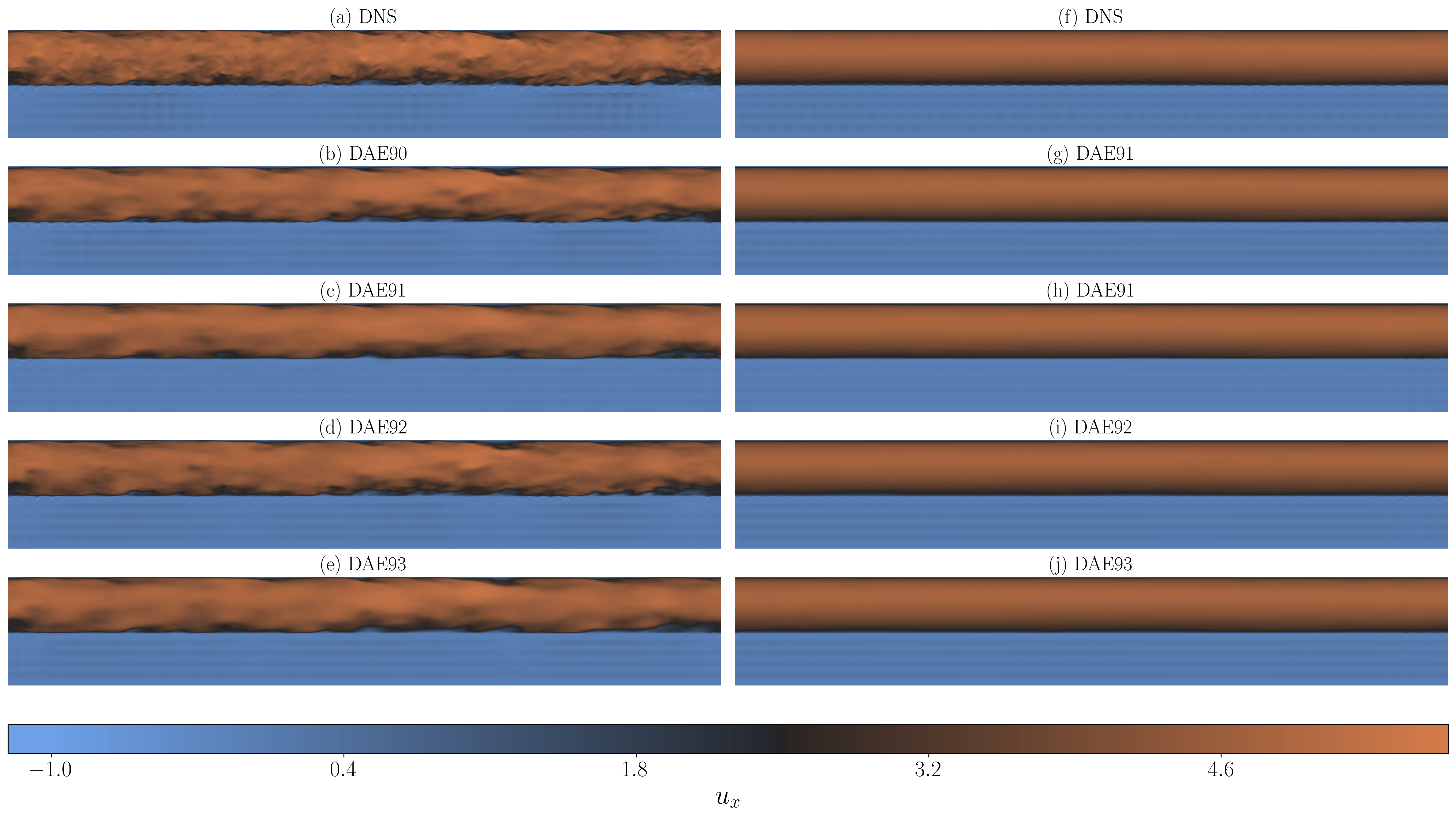
Figure 7: Contours of (a, b, c, d): Instantaneous velocity, (f, g, h, i): Temporal average velocity. Labels are as per Tab. 3

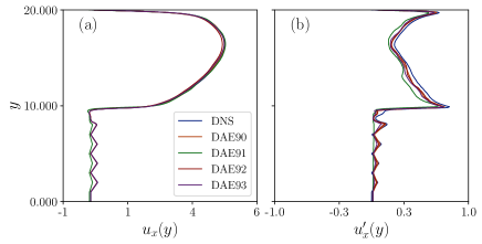
Figure 8: Comparison among ground truth (DNS), reduced order model (DAE) and temporal model for DAE modes using ESN. (a): Average fields (b) Fluctuations

5 Computational performance

The supercomputing systems used for the DNS was HAWK located at the High Performance Computer Center Stuttgart (HLRS). The new flagship machine HAWK, based on the Hewlett Packard Enterprise platform running AMD EPYC 7742 processor code named Rome, has a theoretical peak performance of 26 petaFLOPs, and consists of a 5,632-node cluster. One AMD EPYC 7742 CPU consists of 64 cores, which leads to 128 cores on a single node sharing 256 GB memory on board. This means that a total of 720,896 cores are available on the HAWK system.

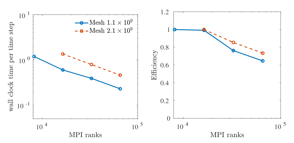
Figure 9: Strong scaling behavior of the solver on ‘HAWK’, wall clock time per time step on the left side. On the right side the efficiency for different numbers of MPI ranks.

The scalability of our direct numerical simulations, employing a high-order solver, was thoroughly evaluated on the advanced HPC system, HAWK, utilizing CPU cores ranging from 8,192 to 65,536. By leveraging ample computational resources, we achieved remarkable performance, with a wall clock time per time step ranging from 0.2 to 0.4 seconds. This optimal computational efficiency enables efficient direct numerical simulations of turbulent flows. Notably, when utilizing the maximal number of MPI ranks, our simulations demonstrated a minimum efficiency of 70$\%$. This achievement highlights the exceptional scalability of our high-order solver on the state-of-the-art HPC cluster, HAWK, setting it apart from previous scalability tests conducted on the low-order Finite Volume Method (FVM) code OpenFOAM Evrim et al (2020); Chu et al (2016b, a); Pandey et al (2017a, 2018b, 2018a); Yang et al (2020) using earlier HPC machines at HLRS. Our findings underscore the outstanding scalability exhibited by our current high-order solver on the advanced HPC system, offering enhanced capabilities for conducting direct numerical simulations. This scalability is crucial for effectively studying turbulent flows and holds significant promise for advancing research in the field.

6 Conclusions

Our study introduces a combined Convolutional Deep Autoencoder–Echo State Network (CDAE-ESN) model as a powerful tool for directly analyzing and forecasting the dynamics and low-order statistics of coupled turbulent channel-porous media flows. The significance of such a flow model lies in its applicability to various industrial systems, including transpiration cooling and smart interface engineering. We used fully-resolved direct numerical simulation to generate the data. By integrating deep autoencoder and echo state network techniques, we overcome the challenges posed by the complex geometry of coupled flow systems, enabling effective modeling and prediction of dominant flow behaviors, particularly within the laminar regime of the porous domain. The obtained results demonstrate the capability of our proposed approach to capture and represent the intricate flow dynamics. Furthermore, to broaden the model’s applicability, we conducted fine-tuning on a dataset with varying porosity. This step aimed to enhance the generalizability of the CDAE-ESN model across a wider range of data domains. The reasonable agreement observed in the average statistics further validates the robustness and versatility of our approach. In summary, the combined CDAE-ESN model presents a promising avenue for analyzing and predicting the behavior of coupled turbulent channel-porous media flows. Its potential applications in diverse industrial systems underscore its significance and highlight the future prospects for incorporating such data-driven models in fluid mechanics research.

7 Acknowledgement

The study has been financially supported by SimTech (EXC 2075/1–390740016) and SFB-1313 (Project No.327154368) from Deutsche Forschungsgemeinschaft (DFG). The financial support by the Deutsche Forschungsgemeinschaft with Grant No. SCHU 1410/30-1 and in parts by the project “DeepTurb – Deep Learning in and of Turbulence” by the Carl Zeiss Foundation is deeply appreciated. The authors gratefully appreciate the access to the high performance computing facility Hawk at HLRS, Stuttgart of Germany. We would like to extend our sincere appreciation to Prof. Jörg Schumacher for his fruitful discussions.

References

- Cantwell et al (2011) Cantwell CD, Sherwin SJ, Kirby RM, Kelly PH (2011) From h to p efficiently: Strategy selection for operator evaluation on hexahedral and tetrahedral elements. Computers & Fluids 43(1):23–28
- Chu et al (2016a) Chu X, Laurien E, McEligot DM (2016a) Direct numerical simulation of strongly heated air flow in a vertical pipe. International Journal of Heat and Mass Transfer 101:1163–1176
- Chu et al (2016b) Chu X, Laurien E, Pandey S (2016b) Direct numerical simulation of heated pipe flow with strong property variation. In: High Performance Computing in Science and Engineering´ 16, Springer, pp 473–486
- Chu et al (2018a) Chu X, Chang W, Pandey S, Luo J, Weigand B, Laurien E (2018a) A computationally light data-driven approach for heat transfer and hydraulic characteristics modeling of supercritical fluids: From dns to dnn. International Journal of Heat and Mass Transfer 123:629–636
- Chu et al (2018b) Chu X, Weigand B, Vaikuntanathan V (2018b) Flow turbulence topology in regular porous media: From macroscopic to microscopic scale with direct numerical simulation. Physics of Fluids 30(6):065,102
- Chu et al (2019) Chu X, Yang G, Pandey S, Weigand B (2019) Direct numerical simulation of convective heat transfer in porous media. International Journal of Heat and Mass Transfer 133:11–20
- Chu et al (2020) Chu X, Wu Y, Rist U, Weigand B (2020) Instability and transition in an elementary porous medium. Physical Review Fluids 5(4):044,304
- Chu et al (2021a) Chu X, Müller J, Weigand B (2021a) Interface-resolved direct numerical simulation of turbulent flow over porous media. In: High Performance Computing in Science and Engineering ’19, Springer International Publishing, pp 343–354
- Chu et al (2021b) Chu X, Wang W, Yang G, Terzis A, Helmig R, Weigand B (2021b) Transport of turbulence across permeable interface in a turbulent channel flow: interface-resolved direct numerical simulation. Transport in Porous Media 136(1):165–189
- Evrim et al (2020) Evrim C, Chu X, Laurien E (2020) Analysis of thermal mixing characteristics in different t-junction configurations. International Journal of Heat and Mass Transfer 158:120,019
- Fang et al (2019) Fang R, Sondak D, Protopapas P, Succi S (2019) Neural network models for the anisotropic Reynolds stress tensor in turbulent channel flow. J Turb pp 1–19
- He et al (2021) He X, Zhao K, Chu X (2021) Automl: A survey of the state-of-the-art. Knowledge-Based Systems 212:106,622
- Karniadakis et al (2005) Karniadakis GE, Karniadakis G, Sherwin S (2005) Spectral/hp element methods for computational fluid dynamics. Oxford University Press on Demand
- Karra et al (2022) Karra SK, Apte SV, He X, Scheibe TD (2022) Pore-resolved simulations of turbulent boundary layer flow over permeable and impermeable sediment beds. arXiv preprint arXiv:220413875
- Kutz et al (2016) Kutz JN, Brunton SL, Brunton BW, Proctor JL (2016) Dynamic mode decomposition: data-driven modeling of complex systems. SIAM
- Nakamura et al (2021) Nakamura T, Fukami K, Hasegawa K, Nabae Y, Fukagata K (2021) Convolutional neural network and long short-term memory based reduced order surrogate for minimal turbulent channel flow. Physics of Fluids 33(2):025,116
- Pandey and Schumacher (2020) Pandey S, Schumacher J (2020) Reservoir computing model of two-dimensional turbulent convection. Physical Review Fluids 5(11):113,506
- Pandey et al (2017a) Pandey S, Chu X, Laurien E (2017a) Investigation of in-tube cooling of carbon dioxide at supercritical pressure by means of direct numerical simulation. International Journal of Heat and Mass Transfer 114:944–957
- Pandey et al (2017b) Pandey S, Laurien E, Chu X (2017b) A modified convective heat transfer model for heated pipe flow of supercritical carbon dioxide. International Journal of Thermal Sciences 117:227–238
- Pandey et al (2018a) Pandey S, Chu X, Laurien E (2018a) Numerical analysis of heat transfer during cooling of supercritical fluid by means of direct numerical simulation. In: High Performance Computing in Science and Engineering’17, pp 241–254
- Pandey et al (2018b) Pandey S, Chu X, Laurien E, Weigand B (2018b) Buoyancy induced turbulence modulation in pipe flow at supercritical pressure under cooling conditions. Physics of Fluids 30(6):065,105
- Pandey et al (2020a) Pandey S, Chu X, Weigand B, Laurien E, Schumacher J (2020a) Relaminarized and recovered turbulence under nonuniform body forces. Physical Review Fluids 5(10):104,604
- Pandey et al (2020b) Pandey S, Schumacher J, Sreenivasan KR (2020b) A perspective on machine learning in turbulent flows. Journal of Turbulence 21(9-10):567–584
- Pandey et al (2022) Pandey S, Teutsch P, Mäder P, Schumacher J (2022) Direct data-driven forecast of local turbulent heat flux in rayleigh–bénard convection. Physics of Fluids 34(4):045,106
- Shen et al (2020) Shen G, Yuan J, Phanikumar MS (2020) Direct numerical simulations of turbulence and hyporheic mixing near sediment water interfaces. Journal of Fluid Mechanics 892:A20
- Solomatine et al (2008) Solomatine D, See LM, Abrahart R (2008) Data-driven modelling: concepts, approaches and experiences. Practical hydroinformatics: Computational intelligence and technological developments in water applications pp 17–30
- Storcheus et al (2015) Storcheus D, Rostamizadeh A, Kumar S (2015) A survey of modern questions and challenges in feature extraction. In: Feature Extraction: Modern Questions and Challenges, PMLR, pp 1–18
- Suga et al (2020) Suga K, Okazaki Y, Kuwata Y (2020) Characteristics of turbulent square duct flows over porous media. Journal of Fluid Mechanics 884
- Terzis et al (2019) Terzis A, Zarikos I, Weishaupt K, Yang G, Chu X, Helmig R, Weigand B (2019) Microscopic velocity field measurements inside a regular porous medium adjacent to a low reynolds number channel flow. Physics of Fluids 31(4):042,001
- Wang et al (2021a) Wang W, Chu X, Lozano-Durán A, Helmig R, Weigand B (2021a) Information transfer between turbulent boundary layer and porous media. Journal of Fluid Mechanics 920:A21
- Wang et al (2021b) Wang W, Yang G, Evrim C, Terzis A, Helmig R, Chu X (2021b) An assessment of turbulence transportation near regular and random permeable interfaces. Physics of Fluids 33(11):115,103
- Wang et al (2022) Wang W, Lozano-Durán A, Helmig R, Chu X (2022) Spatial and spectral characteristics of information flux between turbulent boundary layers and porous media. Journal of Fluid Mechanics 949:A16
- Yang et al (2020) Yang G, Chu X, Vaikuntanathan V, Wang S, Wu J, Weigand B, Terzis A (2020) Droplet mobilization at the walls of a microfluidic channel. Physics of Fluids 32(1):012,004
- Yosinski et al (2014) Yosinski J, Clune J, Bengio Y, Lipson H (2014) How transferable are features in deep neural networks? Advances in neural information processing systems 27
- Zhuang et al (2020) Zhuang F, Qi Z, Duan K, Xi D, Zhu Y, Zhu H, Xiong H, He Q (2020) A comprehensive survey on transfer learning. Proceedings of the IEEE 109(1):43–76