VMC: Video Motion Customization using Temporal Attention Adaption for Text-to-Video Diffusion Models

Abstract

Text-to-video diffusion models have advanced video generation significantly. However, customizing these models to generate videos with tailored motions presents a substantial challenge. In specific, they encounter hurdles in (a) accurately reproducing motion from a target video, and (b) creating diverse visual variations. For example, straightforward extensions of static image customization methods to video often lead to intricate entanglements of appearance and motion data. To tackle this, here we present the Video Motion Customization (VMC) framework, a novel one-shot tuning approach crafted to adapt temporal attention layers within video diffusion models. Our approach introduces a novel motion distillation objective using residual vectors between consecutive frames as a motion reference. The diffusion process then preserves low-frequency motion trajectories while mitigating high-frequency motion-unrelated noise in image space. We validate our method against state-of-the-art video generative models across diverse real-world motions and contexts. Our codes, data and the project demo can be found at https://video-motion-customization.github.io.

1 Introduction

The evolution of diffusion models [28, 13, 31] has significantly advanced Text-to-Image (T2I) generation, notably when paired with extensive text-image datasets [25, 3]. While cascaded diffusion pipelines [14, 27, 39, 2, 9, 33, 37] have extended this success to Text-to-Video (T2V) generation, current models lack the ability to replicate specific motions or generate diverse variations of the same motion with distinct visual attributes and backgrounds. Addressing this, we tackle the challenge of Motion Customization [38]—adapting pre-trained Video Diffusion Models (VDM) to produce motion-specific videos in different contexts, while maintaining the same motion patterns of target subjects.

Given a few subject images for reference, appearance customization [8, 23, 26, 24, 19, 35] in generative models aims to fine-tune models to generate subject images in diverse contexts. However, these approaches, despite varying optimization objectives, commonly strive for faithful image (frame) reconstruction by minimizing the $\ell_{2}$-distance between predicted and ground-truth noise. This may lead to the entangled learning of appearance and motion.

To tackle this, we present VMC, a new framework aimed at adapting pre-trained VDM’s temporal attention layers via our proposed Motion Distillation objective. This approach utilizes residual vectors between consecutive (latent) frames to obtain the motion vectors that trace motion trajectories in the target video. Consequently, we fine-tune VDM’s temporal attention layers to align the ground-truth image-space residuals with their denoised estimates, which equivalently aligns predicted and ground-truth source noise differences within VDM. This enables lightweight and fast one-shot training. To further facilitate the appearance-invariant motion distillation, we transform faithful text prompts into appearance-invariant prompts, e.g. "A bird is flying above a lake in the forest" $\rightarrow$ "A bird is flying" in Fig. 1. This encourages the modules to focus on the motion information and ignore others, such as appearance, distortions, background, etc. During inference, our procedure initiates by sampling key-frames using the adapted key-frame generation U-Net, followed by temporal interpolation and spatial super-resolution. To summarize, VMC makes the following key contributions:

• We introduce a novel fine-tuning strategy which focuses solely on temporal attention layers in the key-frame generation module. This enables lightweight training (15GB vRAM) and fast training ($<$ 5 minutes).

• To our knowledge, we mark a pioneering case of fine-tuning only the temporal attention layers in video diffusion models, without optimizing spatial self or cross-attention layers, while achieving successful motion customization.

• We introduce a novel motion distillation objective that leverages the residual vectors between consecutive (latent) frames as motion vectors.

• We present the concept of appearance-invariant prompts, which further facilitates the process of motion learning when combined with our motion distillation loss.

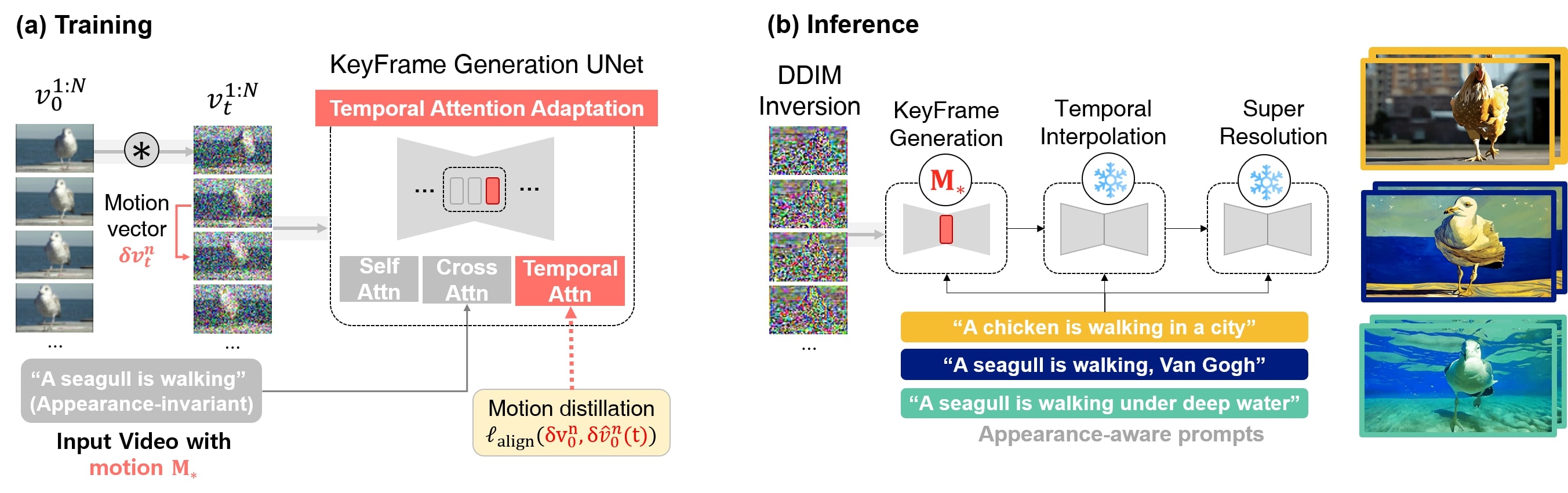
Figure 2: Overview. The proposed Video Motion Customization (VMC) framework distills the motion trajectories from the residual between consecutive (latent) frames, namely motion vector $\delta{\boldsymbol{v}}_{t}^{n}$ for ${\boldsymbol{t}}\geq 0$. We fine-tune only the temporal attention layers of the key-frame generation model by aligning the ground-truth and predicted motion vectors. After training, the customized key-frame generator is leveraged for target motion-driven video generation with new appearances context, e.g. "A chicken is walking in a city".

2 Preliminaries

Diffusion Models.

Diffusion models aim to generate samples from the Gaussian noise through iterative denoising processes. Given a clean sample ${\boldsymbol{x}}_{0}\sim p_{\operatorname{data}}({\boldsymbol{x}})$, the forward process is defined as a Markov chain with forward conditional densities

$$\begin{split}p({\boldsymbol{x}}_{t}\>|\>{\boldsymbol{x}}_{t-1})={\mathcal{N}}({\boldsymbol{x}}_{t}\>|\>\beta_{t}{\boldsymbol{x}}_{t-1},(1-\beta_{t})I)\\ p_{t}({\boldsymbol{x}}_{t}\>|\>{\boldsymbol{x}}_{0})={\mathcal{N}}({\boldsymbol{x}}_{t}\>|\>\sqrt{{\bar{\alpha}}}{\boldsymbol{x}}_{0},(1-{\bar{\alpha}})I),\end{split}$$ (1)

where ${\boldsymbol{x}}_{t}\in\mathbb{R}^{d}$ is a noisy latent variable at a timestep $t$ that has the same dimension as ${\boldsymbol{x}}_{0}$, and $\beta_{t}$ denotes an increasing sequence of noise schedule where $\alpha_{t}\coloneqq 1-\beta_{t}$ and ${\bar{\alpha}}_{t}\coloneqq\Pi_{i=1}^{t}\alpha_{i}$. Then, the goal of diffusion model training is to obtain a residual denoiser ${\boldsymbol{\epsilon}}_{\theta}$:

$$\min_{\theta}{\mathbb{E}}_{{\boldsymbol{x}}_{t}\sim p_{t}({\boldsymbol{x}}_{t}\>|\>{\boldsymbol{x}}_{0}),{\boldsymbol{x}}_{0}\sim p_{\operatorname{data}}({\boldsymbol{x}}_{0}),{\boldsymbol{\epsilon}}\sim{\mathcal{N}}(0,I)}\big{[}\left\lVert{\boldsymbol{\epsilon}}_{\theta}({\boldsymbol{x}}_{t},t)-{\boldsymbol{\epsilon}}\right\rVert\big{]}.$$ (2)

It can be shown that this epsilon matching in (2) is equivalent to the Denoising Score Matching (DSM [16, 30]) with different parameterization:

$$\min_{\theta}{\mathbb{E}}_{{\boldsymbol{x}}_{t},{\boldsymbol{x}}_{0},{\boldsymbol{\epsilon}}}\big{[}\left\lVert\boldsymbol{s}_{\theta}^{t}({\boldsymbol{x}}_{t})-\nabla_{{\boldsymbol{x}}_{t}}\log p_{t}({\boldsymbol{x}}_{t}\>|\>{\boldsymbol{x}}_{0})\right\rVert\big{]},$$ (3)

where $\boldsymbol{s}_{\theta^{*}}({\boldsymbol{x}}_{t},t)\simeq-\frac{{\boldsymbol{x}}_{t}-\sqrt{{\bar{\alpha}}_{t}}{\boldsymbol{x}}_{0}}{1-{\bar{\alpha}}}=-\frac{1}{\sqrt{1-{\bar{\alpha}}_{t}}}{\boldsymbol{\epsilon}}_{\theta^{*}}({\boldsymbol{x}}_{t},t)$. The reverse sampling from $q({\boldsymbol{x}}_{t-1}|{\boldsymbol{x}}_{t},{\boldsymbol{\epsilon}}_{\theta^{*}}({\boldsymbol{x}}_{t},t))$ is then achieved by

$${\boldsymbol{x}}_{t-1}=\frac{1}{\sqrt{\alpha_{t}}}\Big{(}{\boldsymbol{x}}_{t}-\frac{1-\alpha_{t}}{\sqrt{1-\bar{\alpha}_{t}}}\boldsymbol{\epsilon}_{\theta^{*}}({\boldsymbol{x}}_{t},t)\Big{)}+\tilde{\beta}_{t}{\boldsymbol{\epsilon}},$$ (4)

where ${\boldsymbol{\epsilon}}\sim{\mathcal{N}}(0,{\boldsymbol{I}})$ and $\tilde{\beta}_{t}\coloneqq\frac{1-{\bar{\alpha}}_{t-1}}{1-{\bar{\alpha}}_{t}}\beta_{t}$. To accelerate sampling, DDIM [29] further proposes another sampling method as follows:

$${\boldsymbol{x}}_{t-1}=\sqrt{{\bar{\alpha}}_{t-1}}\hat{{\boldsymbol{x}}}_{0}(t)+\sqrt{1-{\bar{\alpha}}_{t-1}-\eta^{2}\tilde{\beta_{t}}^{2}}{\boldsymbol{\epsilon}}_{\theta^{*}}({\boldsymbol{x}}_{t},t)+\eta\tilde{\beta}_{t}{\boldsymbol{\epsilon}},$$ (5)

where $\eta\in[0,1]$ is a stochasticity parameter, and $\hat{{\boldsymbol{x}}}_{0}(t)$ is the denoised estimate which can be equivalently derived using Tweedie’s formula [6]:

$$\hat{{\boldsymbol{x}}}_{0}(t)\coloneqq\frac{1}{\sqrt{{\bar{\alpha}}_{t}}}({\boldsymbol{x}}_{t}-\sqrt{1-{\bar{\alpha}}_{t}}{\boldsymbol{\epsilon}}_{\theta^{*}}({\boldsymbol{x}}_{t},t)).$$ (6)

For a text-guided Diffusion Model, the training objective is often given by:

$$\min_{\theta}{\mathbb{E}}_{{\boldsymbol{x}}_{t},{\boldsymbol{x}}_{0},{\boldsymbol{\epsilon}},c}\big{[}\left\lVert{\boldsymbol{\epsilon}}_{\theta}({\boldsymbol{x}}_{t},t,c)-{\boldsymbol{\epsilon}}\right\rVert\big{]},$$ (7)

where $c$ represents the textual embedding. Throughout this paper, we will often omit $c$ from ${\boldsymbol{\epsilon}}_{\theta}({\boldsymbol{x}}_{t},t,c)$ if it does not lead to notational ambiguity.

Video Diffusion Models.

Video diffusion models [14, 37, 12] further attempt to model the video data distribution. Specifically, Let $({\boldsymbol{v}}^{n})_{n\in\{1,\dots,N\}}$ represents the $N$-frame input video sequence. Then, for a given $n$-th frame ${\boldsymbol{v}}^{n}\in\mathbb{R}^{d}$, let ${\boldsymbol{v}}^{1:N}\in\mathbb{R}^{N\times d}$ represents a whole video vector. Let $\boldsymbol{v}_{t}^{n}=\sqrt{\bar{\alpha}_{t}}\boldsymbol{v}^{n}+\sqrt{1-\bar{\alpha}_{t}}\boldsymbol{\epsilon}_{t}^{n}$ represents the $n$-th noisy frame latent sampled from $p_{t}(\boldsymbol{v}_{t}^{n}|\boldsymbol{v}^{n})$, where $\boldsymbol{\epsilon}_{t}^{n}\sim\mathcal{N}(0,I)$. We similarly define $({\boldsymbol{v}}_{t}^{n})_{n\in 1,\dots,N}$, ${\boldsymbol{v}}_{t}^{1:N}$, and ${\boldsymbol{\epsilon}}_{t}^{1:N}$. The goal of video diffusion model training is then to obtain a residual denoiser ${\boldsymbol{\epsilon}}_{\theta}$ with textual condition $c$ and video input that satisfies:

$$\min_{\theta}{\mathbb{E}}_{{\boldsymbol{v}}_{t}^{1:N},{\boldsymbol{v}}^{1:N},{\boldsymbol{\epsilon}}_{t}^{1:N},c}\big{[}\left\lVert{\boldsymbol{\epsilon}}_{\theta}({\boldsymbol{v}}_{t}^{1:N},t,c)-{\boldsymbol{\epsilon}}_{t}^{1:N}\right\rVert\big{]},$$ (8)

where ${\boldsymbol{\epsilon}}_{\theta}({\boldsymbol{v}}_{t}^{1:N},t,c),{\boldsymbol{\epsilon}}_{t}^{1:N}\in\mathbb{R}^{N\times d}$. In this work, we denote the predicted noise of $n$-th frame as ${\boldsymbol{\epsilon}}_{\theta}^{n}({\boldsymbol{v}}_{t}^{1:N},t,c)\in\mathbb{R}^{d}$.

In practice, contemporary video diffusion models often employ cascaded inference pipelines for high-resolution outputs. For instance, [37] initially generates a low-resolution video with strong text-video correlation, further enhancing its resolution via temporal interpolation and spatial super-resolution modules.

In exploring video generative tasks through diffusion models, two primary approaches have emerged: foundational Video Diffusion Models (VDMs) or leveraging pre-trained Text-to-Image (T2I) models. To extend image diffusion models to videos, several architectural modifications are made. Typically, U-Net generative modules integrate temporal attention blocks after spatial attentions [12]. Moreover, 2D convolution layers are inflated to 3D convolution layers by altering kernels [12].

3 Video Motion Customization

Given an input video, our main goal is to (a) distill the motion patterns $M_{*}$ of target subjects, and (b) customize the input video in different contexts while maintaining the same motion patterns $M_{*}$, e.g. Sharks w/ motion $M_{*}$ $\rightarrow$ Airplanes w/ motion $M_{*}$, with minimal computational costs.

To this end, we propose a novel video motion customization framework, namely VMC, which leverages cascaded video diffusion models with robust temporal priors. One notable aspect of the proposed framework is that we perform fine-tuning only on the key-frame generation module, also referred to as the T2V base model, within the cascaded VDMs, which guarantees computational and memory efficiency. Specifically, within the key-frame generation model, our fine-tuning process only targets the temporal attention layers. This facilitates adaptation while preserving the model’s inherent capacity for generic synthesis. Notably, we freeze the subsequent frame interpolation and spatial super-resolution modules as-is (Fig. 2).

3.1 Temporal Attention Adaptation

In order to distill the motion $M_{*}$, we first propose a new objective function for temporal attention adaptation using residual cosine similarity. Our intuition is that residual vectors between consecutive frames may include information about the motion trajectories.

Let $({\boldsymbol{v}}^{n})_{n\in\{1,\dots,N\}}$ represents the $N$-frame input video sequence. As defined in Section 2, for a given noisy video latent vector $\boldsymbol{v}_{t}^{1:N}$ with ${\boldsymbol{\epsilon}}_{t}^{1:N}$, let $\boldsymbol{v}_{t}^{n}$ represents the $n$-th noisy frame latent sampled from $p_{t}(\boldsymbol{v}_{t}^{n}|\boldsymbol{v}^{n})$ with ${\boldsymbol{\epsilon}}_{t}^{n}$. We will interchangeably use ${\boldsymbol{v}}^{n}$ and ${\boldsymbol{v}}_{0}^{n}$ for notational simplicity. Likewise, $\boldsymbol{v}_{t}^{n+c}$ is defined as $\boldsymbol{v}_{t}^{n}$, with $c>0$ representing the fixed frame stride. Then, we define the frame residual vector at time $t\geq 0$ as

$$\delta{\boldsymbol{v}}_{t}^{n}\coloneqq{\boldsymbol{v}}_{t}^{n+c}-{\boldsymbol{v}}_{t}^{n},$$ (9)

where we similarly define the epsilon residual vector $\delta{\boldsymbol{\epsilon}}_{t}^{n}$. In the rest of the paper, we interchangeably use frame residual vector and motion vector.

We expect that these motion vectors may encode information about motion patterns, where such information may vary depending on the time $t$ and its corresponding noise level. The difference vector $\delta{\boldsymbol{v}}_{t}^{n}$ can be delineated as:

$$\begin{split}\delta{\boldsymbol{v}}_{t}^{n}&=\sqrt{{\bar{\alpha}}_{t}}({\boldsymbol{v}}_{0}^{n+c}-{\boldsymbol{v}}_{0}^{n})+\sqrt{1-{\bar{\alpha}}_{t}}({\boldsymbol{\epsilon}}_{t}^{n+c}-{\boldsymbol{\epsilon}}_{t}^{n})\\ &=\sqrt{{\bar{\alpha}}_{t}}\delta{\boldsymbol{v}}_{0}^{n}+\sqrt{1-{\bar{\alpha}}_{t}}\delta{\boldsymbol{\epsilon}}_{t}^{n},\end{split}$$ (10)

where $\delta{\boldsymbol{\epsilon}}_{t}^{n}$ is normally distributed with zero mean and $2I$ variance. In essence, $\delta{\boldsymbol{v}}_{t}^{n}$ can be acquired through the following diffusion kernel:

$$p(\delta{\boldsymbol{v}}_{t}^{n}\>|\>\delta{\boldsymbol{v}}_{0}^{n})={\mathcal{N}}(\delta{\boldsymbol{v}}_{t}^{n}\>|\>\sqrt{{\bar{\alpha}}_{t}}\delta{\boldsymbol{v}}_{0}^{n},2(1-{\bar{\alpha}}_{t})I).$$ (11)

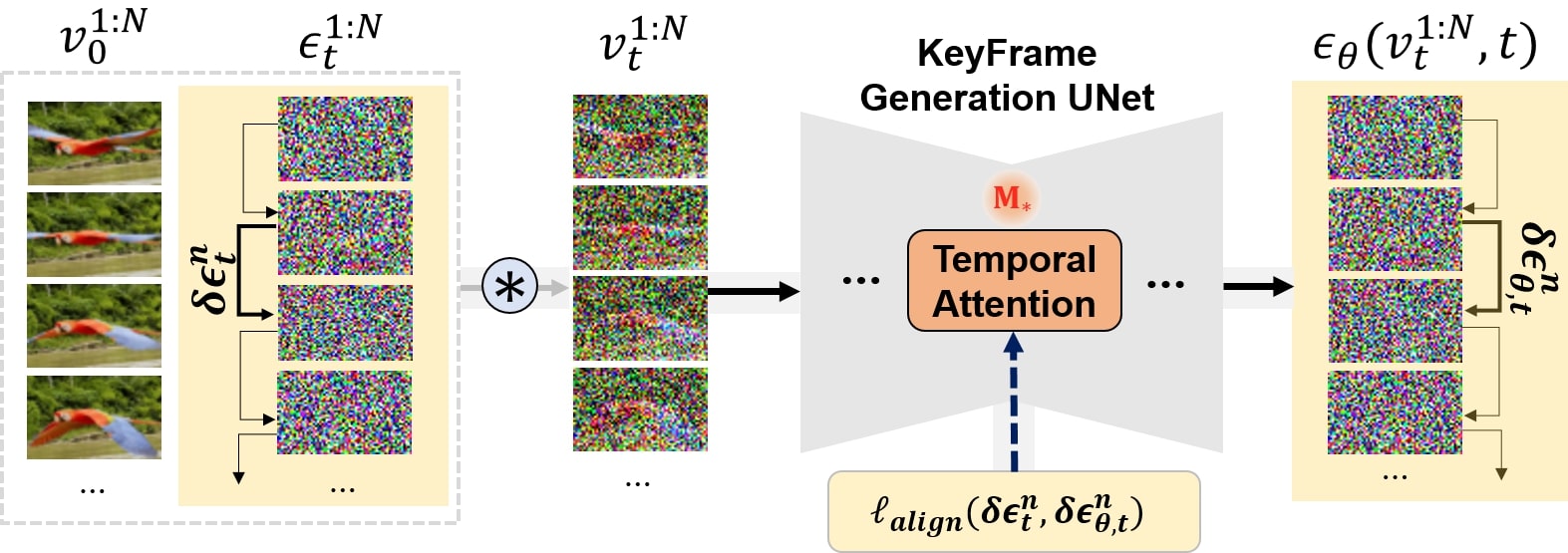
Figure 3: Training. The proposed framework aims to learn motion by $\delta{\boldsymbol{\epsilon}}_{t}^{n}$-alignment using (16) or (17). Note that we only fine-tune the temporal attention layers in the key-frame generation U-Net. The blue circle represents the diffusion forward process.

In light of this, our goal is to transfer motion information to the temporal attention layers by leveraging the motion vectors. For this, we first simulate the motion vectors using video diffusion models. Specifically, as similarly done in (6), the denoised video vector estimates $\hat{{\boldsymbol{v}}}_{0}^{1:N}(t)$ can be derived by applying Tweedie’s formula:

$$\hat{{\boldsymbol{v}}}_{0}^{1:N}(t)\coloneqq\frac{1}{\sqrt{{\bar{\alpha}}_{t}}}\big{(}{\boldsymbol{v}}_{t}^{1:N}-\sqrt{1-{\bar{\alpha}}_{t}}{\boldsymbol{\epsilon}}_{\theta}({\boldsymbol{v}}_{t}^{1:N},t)\big{)},$$ (12)

where $\hat{{\boldsymbol{v}}}_{0}^{1:N}(t)$ is an empirical Bayes optimal posterior expectation $\mathbb{E}[{\boldsymbol{v}}_{0}^{1:N}\>|\>{\boldsymbol{v}}_{t}^{1:N}]$. Then, the denoised motion vector estimate $\delta\hat{{\boldsymbol{v}}}_{0}^{n}$ can be defined in terms of $\delta{\boldsymbol{v}}_{t}^{n}$ and $\delta{\boldsymbol{\epsilon}}_{\theta}^{n}({\boldsymbol{v}}_{t}^{1:N},t)$ by using (12):

$$\delta\hat{{\boldsymbol{v}}}_{0}^{n}(t)\coloneqq\frac{1}{\sqrt{{\bar{\alpha}}_{t}}}\Big{(}\delta{\boldsymbol{v}}_{t}^{n}-\sqrt{1-{\bar{\alpha}}_{t}}\delta{\boldsymbol{\epsilon}}_{\theta,t}^{n}\Big{)},$$ (13)

where $\delta{\boldsymbol{\epsilon}}_{\theta}^{n}({\boldsymbol{v}}_{t}^{1:N},t)\coloneqq{\boldsymbol{\epsilon}}_{\theta}^{n+c}({\boldsymbol{v}}_{t}^{1:N},t)-{\boldsymbol{\epsilon}}_{\theta}^{n}({\boldsymbol{v}}_{t}^{1:N},t)$ is abbreviated as $\delta{\boldsymbol{\epsilon}}_{\theta,t}^{n}$ for notational simplicity. Similarly, one can obtain ground-truth motion vector $\delta{\boldsymbol{v}}_{0}^{n}$ in terms of $\delta{\boldsymbol{v}}_{t}^{n}$ and $\delta{\boldsymbol{\epsilon}}_{t}^{n}$ by using (10):

$$\delta{\boldsymbol{v}}_{0}^{n}=\frac{1}{\sqrt{{\bar{\alpha}}_{t}}}\Big{(}\delta{\boldsymbol{v}}_{t}^{n}-\sqrt{1-{\bar{\alpha}}_{t}}\delta{\boldsymbol{\epsilon}}_{t}^{n}\Big{)}.$$ (14)

Then, our objective is to finetune $\theta$ by aligning the motion vector $\delta{\boldsymbol{v}}_{0}^{n}$ and its denoised estimate $\delta\hat{{\boldsymbol{v}}}_{0}^{n}(t)$:

$$\min_{\theta}\mathbb{E}_{t,n,{\boldsymbol{\epsilon}}_{t}^{n},{\boldsymbol{\epsilon}}_{t}^{n+c}}\Big{[}\ell_{\text{align}}\big{(}\delta{\boldsymbol{v}}_{0}^{n},\delta\hat{{\boldsymbol{v}}}_{0}^{n}(t)\big{)}\Big{]},$$ (15)

with a loss function $\ell_{\text{align}}:\mathbb{R}^{d}\times\mathbb{R}^{d}\rightarrow\mathbb{R}$. By using $\ell_{2}$-distance for $\ell_{\text{align}}$, this is equivalent to matching $\delta{\boldsymbol{\epsilon}}_{\theta,t}^{n}$ and $\delta{\boldsymbol{\epsilon}}_{t}^{n}$:

$$\begin{split}\ell_{\text{align}}\big{(}\delta{\boldsymbol{v}}_{0}^{n},\delta\hat{{\boldsymbol{v}}}_{0}^{n}(t)\big{)}=\frac{1-{\bar{\alpha}}_{t}}{{\bar{\alpha}}_{t}}\left\lVert\delta{\boldsymbol{\epsilon}}_{t}^{n}-\delta{\boldsymbol{\epsilon}}_{\theta,t}^{n}\right\rVert^{2}.\\ \end{split}$$ (16)

Notably, aligning the ground-truth and predicted motion vectors translates into aligning epsilon residuals.

While this objective demonstrates effective empirical performance, our additional observations indicate that using $\ell_{\text{cos}}(\delta{\boldsymbol{\epsilon}}_{t}^{n},\delta{\boldsymbol{\epsilon}}_{\theta,t}^{n})$ may further improve the distillation, where $\ell_{\text{cos}}({\boldsymbol{x}},{\boldsymbol{y}})=1-\frac{\langle{\boldsymbol{x}},{\boldsymbol{y}}\rangle}{\|{\boldsymbol{x}}\|\|{\boldsymbol{y}}\|}$ for ${\boldsymbol{x}},{\boldsymbol{y}}\in\mathbb{R}^{d}$ (more analysis in section 4.3). Accordingly, our optimization framework is finally defined as follows:

$$\min_{\theta}\mathbb{E}_{t,n,{\boldsymbol{\epsilon}}_{t}^{n},{\boldsymbol{\epsilon}}_{t}^{n+c}}[\ell_{\text{cos}}(\delta{\boldsymbol{\epsilon}}_{t}^{n},\delta{\boldsymbol{\epsilon}}_{\theta,t}^{n})].$$ (17)

Thus, the proposed optimization framework aims to maximize the residual cosine similarity between $\delta{\boldsymbol{\epsilon}}_{t}^{n}$ and $\delta{\boldsymbol{\epsilon}}_{\theta,t}^{n}$. In our observation, aligning the image-space residuals ($\delta{\boldsymbol{v}}_{0}^{n}$ and $\delta\hat{{\boldsymbol{v}}}_{0}^{n}(t)$) corresponds to aligning the latent-space epsilon residuals ($\delta{\boldsymbol{\epsilon}}_{t}^{n}$ and $\delta{\boldsymbol{\epsilon}}_{\theta,t}^{n}$) across varying time steps. This relationship stems from expressing the motion vector $\delta{\boldsymbol{v}}_{0}^{n}$ and its estimation $\delta\hat{{\boldsymbol{v}}}_{0}^{n}(t)$ in terms of $\delta{\boldsymbol{v}}_{t}^{n}$, $\delta{\boldsymbol{\epsilon}}_{t}^{n}$, and $\delta{\boldsymbol{\epsilon}}_{\theta,t}^{n}$. Consequently, the proposed optimization framework fine-tunes temporal attention layers by leveraging diverse diffusion latent spaces at time $t$ which potentially contains multi-scale rich descriptions of video frames. Hence, this optimization approach can be seamlessly applied to video diffusion models trained using epsilon-matching, thanks to the equivalence between $\delta{\boldsymbol{\epsilon}}_{t}^{n}$-matching and $\delta{\boldsymbol{v}}_{0}^{n}$-matching. Practically, we exclusively fine-tune the temporal attention layers $\theta_{\text{TA}}\subset\theta$, originally designed for dynamic temporal data assimilation [35]. The frame stride remains fixed at $c=1$ across all experiments.

3.2 Appearance-invariant Prompts

In motion distillation, it is crucial to filter out disruptive variations that are unrelated to motion. These variations may include changes in appearance and background, distortions, consecutive frame inconsistencies, etc. To achieve this, we further utilize appearance-invariant prompts. Diverging from traditional generative customization frameworks [23, 24, 35, 38] that rely on text prompts that “faithfully” describe the input image or video during model fine-tuning, our framework purposedly employs “unfaithful” text prompts during the training phase. Specifically, our approach involves the removal of background information. For instance, the text prompt ‘a cat is roaring on the grass under the tree’ is simplified to ‘a cat is roaring’ as presented in Fig. 4. This reduces background complexity as in Fig. 4a comapred to Fig. 4b, facilitating the application of new appearance in motion distillation.

3.3 Inference Pipeline

Once trained, in the inference phase, our process begins by computing inverted latents from the input video through DDIM inversion. Subsequently, the inverted latents are fed into the temporally fine-tuned keyframe generation model, yielding short and low-resolution keyframes. These keyframes then undergo temporal extension using the unaltered frame interpolation model. Lastly, the interpolated frames are subjected to spatial enlargement through the spatial super-resolution model. Overview of the process is depicted in Fig. 2.

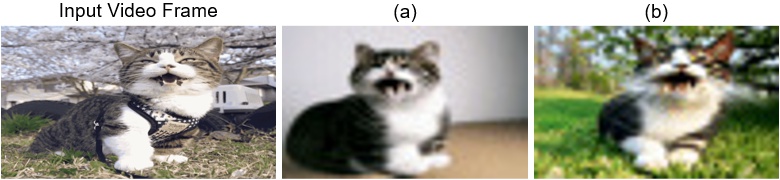
Figure 4: Appearance-invariant Prompt. Comparison of input reconstruction with and without appearance-invariant prompt: (a) and (b) depict sampled low-resolution (64x40) keyframes. For (a), the training prompt used was “A cat is roaring,” while for (b), the training prompt was “A cat is roaring on the grass under the tree.” Our appearance-invariant prompt enables the removal of background information that can disturb motion distillation.

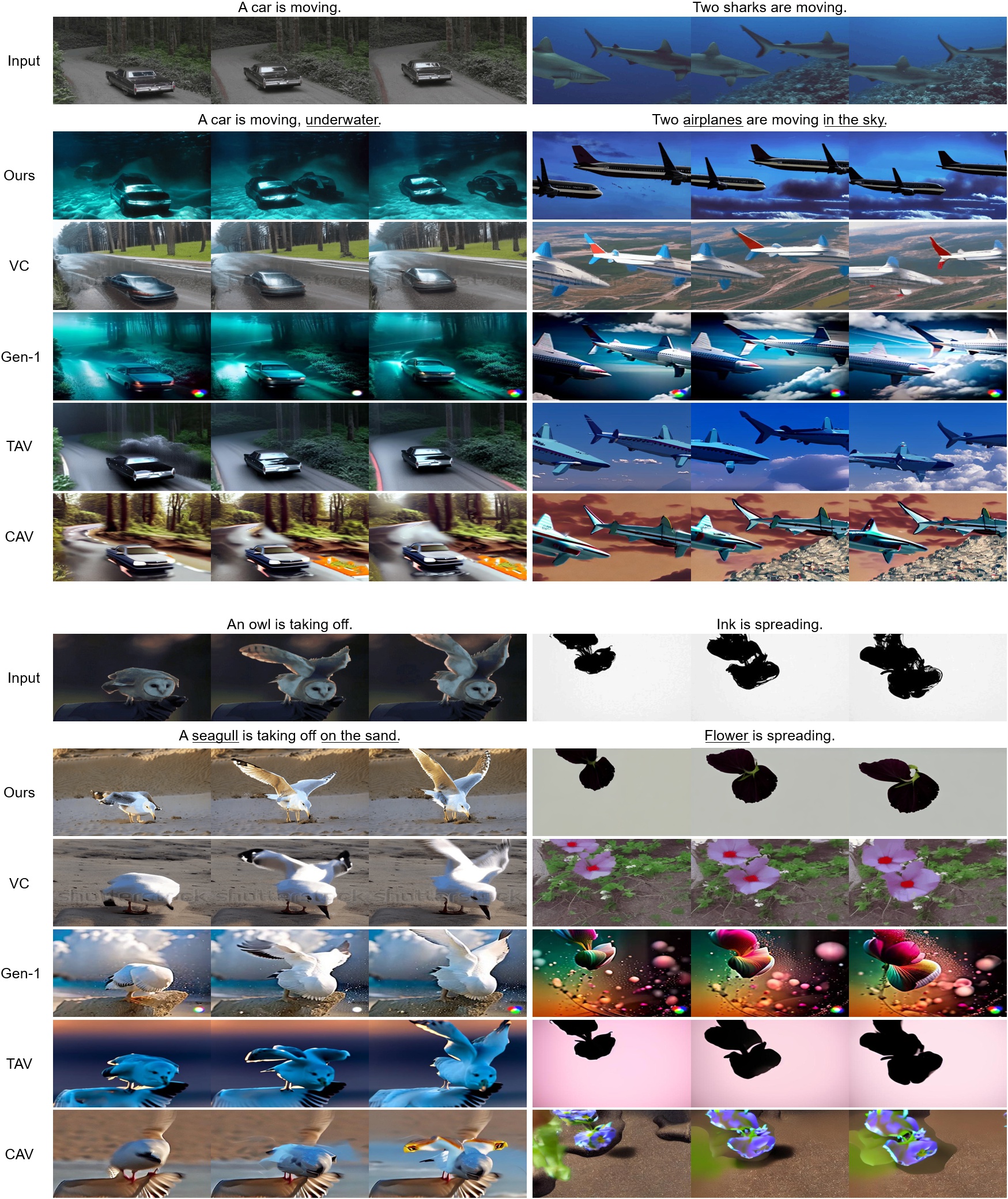
Figure 5: Qualitative comparison against state-of-the-art baselines. In contrast to other baselines, the proposed framework succeeds in motion-driven customization, even for difficult compositional customization.

4 Experiments

4.1 Implementation Details

In our experiments, we choose Show-1 [37] as our VDM backbone and its publicly available pre-trained weights . All experiments were conducted using a single NVIDIA RTX 6000 GPU. VMC with Show-1 demonstrates efficient resource usage, requiring only 15GB of vRAM during mixed-precision training [20], which is completed within 5 minutes. During inference, generating a single video comprising 29 frames at a resolution of 576 x 320 consumes 18GB of vRAM and takes approximately 12 minutes.

4.2 Baseline Comparisons

Dataset Selection. In our experiments, we draw upon a dataset that comprises 24 videos. These videos encompass a broad spectrum of motion types occurring in various contexts, encompassing vehicles, humans, birds, plants, diffusion processes, mammals, sea creatures, and more. This diversity provides a comprehensive range of motion scenarios for our assessment. Out of these 24 videos, 13 are sourced from the DAVIS dataset [21], 10 from the WebVid dataset [1], and 1 video is obtained from LAMP [36].

Baselines.

Our method is compared against four contemporary baselines that integrate depth map signals into the diffusion denoising process to assimilate motion information. Notably, our approach operates without the necessity of depth maps during both training and inference, in contrast to these baseline methods.

Specifically, VideoComposer (VC) [32] is an open-source latent-based video diffusion model tailored for compositional video generation tasks. Gen-1 [7] introduces a video diffusion architecture incorporating additional structure and content guidance for video-to-video translation. In contrast to our targeted fine-tuning of temporal attention, Tune-A-Video (TAV) [35] fine-tunes self, cross, and temporal attention layers within a pre-trained, but inflated T2I model on input videos. Control-A-Video (CAV) [5] introduces a controllable T2V diffusion model utilizing control signals and a first-frame conditioning strategy. Notably, while closely aligned with our framework, Motion Director [38] lacks available code at the time of our research.

Qualitative Results.

We offer visual comparisons of our method against four baselines in Fig. 5. The compared baselines face challenges in adapting the motion of the input video to new contexts. They exhibit difficulties in applying the overall motion, neglecting the specific background indicated in the target text (e.g., “underwater” or “on the sand”). Additionally, they face difficulties in deviating from the original shape of the subject in the input video, leading to issues like a shark-shaped airplane, an owl-shaped seagull, or preservation of the shape of the ground where a seagull is taking off. In contrast, the proposed framework succeeds in motion-driven customization, even for difficult compositional customization, e.g. Two sharks are moving. $\rightarrow$ Two airplanes are moving in the sky.

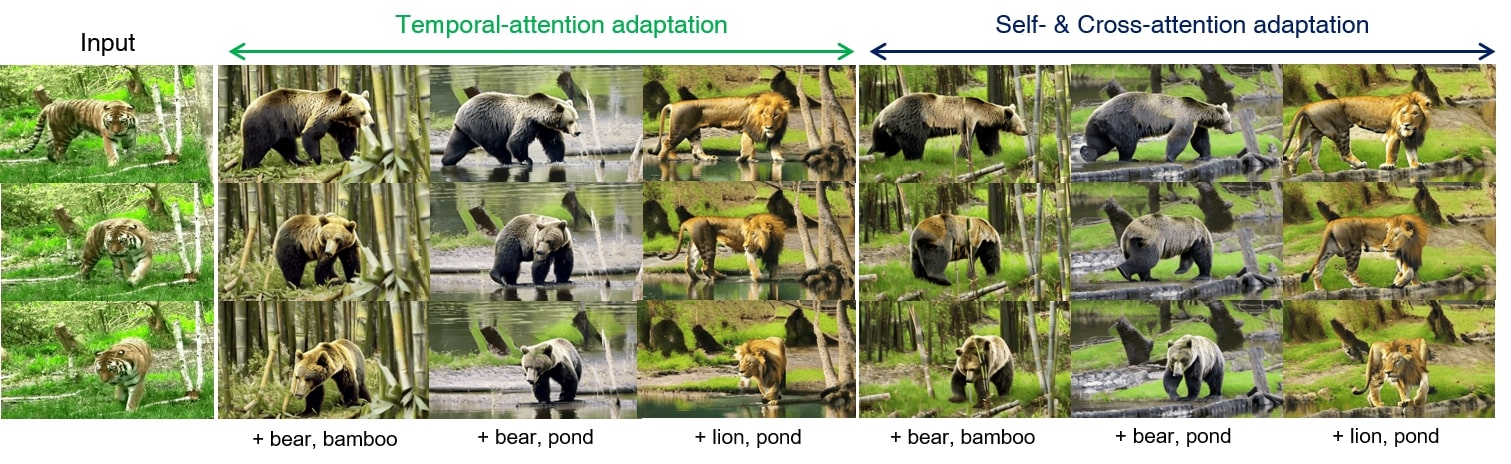
Figure 6: Comparative analysis of the proposed frameworks with fine-tuning (a) temporal attention and (b) self- and cross-attention layers.

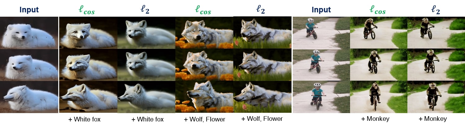
Figure 7: Comparative analysis of the proposed frameworks with (a) $\ell_{cos}$ and (b) $\ell_{2}$ loss functions.

Quantitative Results.

We further quantitatively demonstrate the effectiveness of our method against the baselines through automatic metrics and user study.

Automatic Metrics. We use CLIP [22] encoders for automatic metrics. For textual alignment, we compute the average cosine similarity between the target prompt and the generated frames. In terms of frame consistency, we obtain CLIP image features within the output video and then calculate the average cosine similarity among all pairs of video frames. For methods that generate temporally interpolated frames, we utilized the keyframe indexes to calculate the metric for a fair evaluation. To illustrate, in the case of VMC, which takes an 8-frame input and produces a 29-frame output, we considered the frames at the following indexes: 1, 5, 9, 13, 17, 21, 25, 29. As shown in Table 1, VMC outperforms baselines in both text alignment and temporal consistency.

User Study. We conducted a survey involving a total of 27 participants to assess four key aspects: the preservation of motion between the input video and the generated output video, appearance diversity in the output video compared to the input video, the text alignment with the target prompt, and the overall consistency of the generated frames. The survey utilized a rating scale ranging from 1 to 5. For assessing motion preservation, we employed the question: “To what extent is the motion of the input video retained in the output video?” To evaluate appearance diversity, participants were asked: “To what extent does the appearance of the output video avoid being restricted on the input video’s appearance?” Tab. 1 shows that our method surpasses the baselines in all four aspects.

	Text	Temporal	Motion	Appearance	Text	Temporal
	Alignment	Consistency	Preservation	Diversity	Alignment	Consistency
VC	0.798	0.958	3.45	3.43	2.96	3.03
Gen-1	0.780	0.957	3.46	3.17	2.87	2.73
TAV	0.758	0.947	3.50	2.88	2.67	2.80
CAV	0.764	0.952	2.75	2.45	2.07	2.00
Ours	0.801	0.959	4.42	4.54	4.56	4.57

Table 1: Quantitative evaluation using CLIP and user study. Our method significantly outperforms the other baselines.

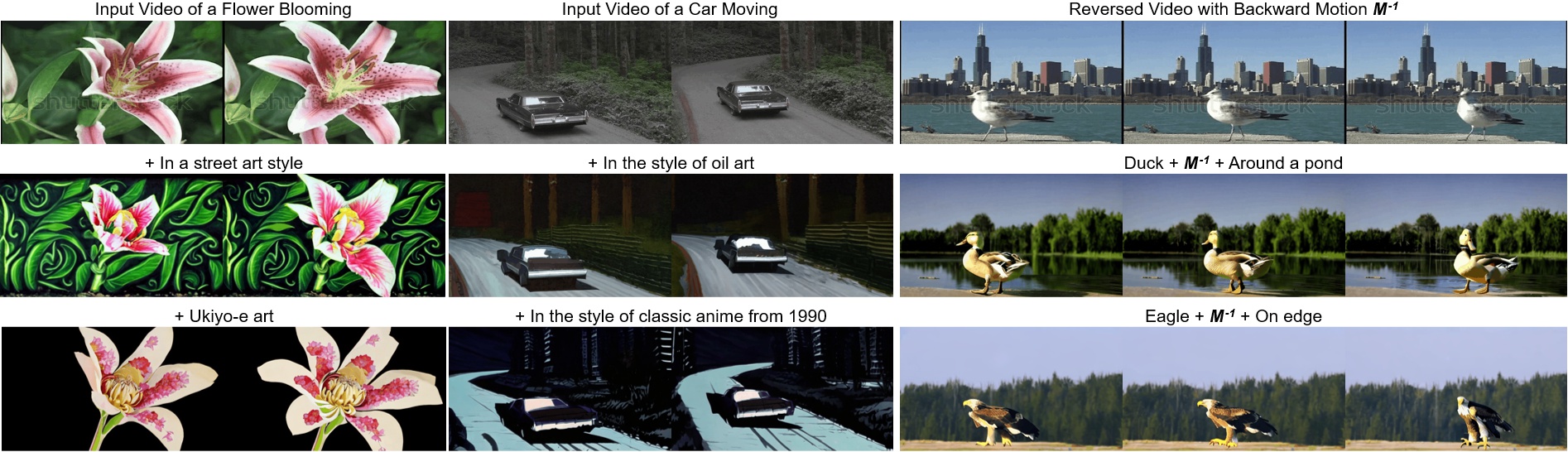
Figure 8: Left: Style transfer on two videos. Right: Motion customization results on the video of “A seagull is walking backward.”

4.3 Ablation Studies

Comparisons on attention layers. We conducted a comparative study evaluating the performance of fine-tuning: (a) temporal attention layers and (b) self- and cross-attention layers. Illustrated in Fig. 6, both frameworks exhibit proficient motion learning capabilities. Notably, the utilization of customized temporal attention layers (a) yields smoother frame transitions, indicating the effectiveness of the optimization framework (17) in encouraging motion distillation, with a slight preference observed for customized temporal attention layers.

This observation stems from the premise that integrating the proposed motion distillation objective (17) may autonomously and accurately embed motion information within temporal attention layers [12, 14]. This suggests a potential application of the motion distillation objective for training large-scale video diffusion models, warranting further exploration in future research endeavors.

Choice of loss functions.

In addition, we conducted a comparative analysis on distinct training loss functions in (17): the $\ell_{2}$-distance and $\ell_{cos}$ as delineated in (17). As depicted in Fig. 7, the $\delta{\boldsymbol{\epsilon}}$-matching process in (15) and (17) demonstrates compatibility with generic loss functions. While both $\ell_{2}(\delta{\boldsymbol{\epsilon}}_{t}^{n},\delta{\boldsymbol{\epsilon}}_{\theta,t}^{n})$ and $\ell_{cos}(\delta{\boldsymbol{\epsilon}}_{t}^{n},\delta{\boldsymbol{\epsilon}}_{\theta,t}^{n})$ are promising objectives, the marginal superiority of $\ell_{cos}(\delta{\boldsymbol{\epsilon}}_{t}^{n},\delta{\boldsymbol{\epsilon}}_{\theta,t}^{n})$ led to its adoption for visualizations in this study.

Importance of adaptation.

To assess the importance of temporal attention adaptation, we conducted a visualization of customized generations without temporal attention adaptation, as detailed in Section 3.1. Specifically, from our original architecture in Fig. 2, we omitted attention adaptation and performed inference by maintaining the U-Net modules in a frozen state. The outcomes depicted in Fig. 9 indicate that while DDIM inversion guides the generations to mimic the motion of the input video, it alone does not ensure successful motion distillation. The observed changes in appearance and motion exhibit an entangled relationship. Consequently, this underlines the necessity of an explicit motion distillation objective to achieve consistent motion transfer, independent of any alterations in appearance.

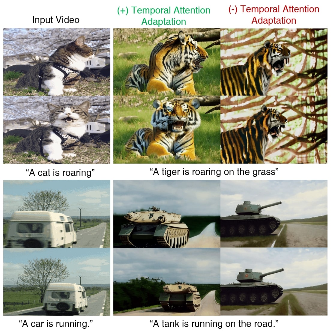
Figure 9: Ablation study on temporal attention adaptation. Without temporal attention adaptation, motion distillation fails.

4.4 Additional results

Video Style Transfer. We illustrate video style transfer applications in Fig. 8-Left. We incorporate style prompts at the end of the text after applying appearance-invariant prompting (see Section 3.2). Target styles are fluidly injected while preserving the distilled motion of an input video.

Learning Backward Motion. To further verify our video motion customization capabilities, we present a challenging scenario: extracting backward motion from a reversed video sequence where frames are arranged in reverse order. This scenario, an exceedingly rare event in real-world videos, is highly improbable within standard training video datasets [1]. Illustrated in Fig. 8, our VMC framework showcases proficiency in learning “a bird walking backward” motion and generating diverse videos with distinct subjects and backgrounds. This capability not only enables leveraging the distilled motion but also offers prospects for further contextual editing.

5 Conclusion

This paper introduces Video Motion Customization (VMC), addressing challenges in adapting Text-to-Video (T2V) models to generate motion-driven diverse visual customizations. Existing models struggle with accurately replicating motion from a target video and creating varied visual outputs, leading to entanglements of appearance and motion data. To overcome this, our VMC framework presents a novel one-shot tuning approach, focusing on adapting temporal attention layers within video diffusion models. This framework stands out for its efficiency in time and memory, ease of implementation, and minimal hyperparameters. We demonstrated the efficacy of our customization methods across diverse motion types, appearances, and contexts.

Ethics Statement. Our work is based on a generative model with potential for misuse, including the creation of deceptive content, which may have negative societal impacts. Additionally, inappropriate content and biases could be included in the datasets used for the foundational training.

Appendix A Appendix

The supplementary sections in Appendix are organized as follows. Section B introduces the pseudo training algorithm behind our Video Motion Customization (VMC) framework. In Section C, we provide a discussion on related works in the field of generative model customization. Following this, we delve into the details on our training and inference configurations in Section D. Concluding the document, Section E features a showcase of additional results obtained from our VMC framework.

Appendix B Pseudo Training Algorithm

Algorithm 1 Temporal Attention Adaption

1:Input: $N$-frame input video sequence $({\boldsymbol{v}}_{0}^{n})_{n\in\{1,\dots,N\}}$, appearance-invariant training prompt ${\mathcal{P}}_{\text{inv}}$, textual encoder $\psi$, Training iterations $M$, key-frame generator parameterized by $\theta$ and its temporal attention parameters $\theta_{\text{TA}}$.

2:Output: Fine-tuned temporal attention layers $\theta_{\text{TA}}^{*}$.

3:

4:for $step=1$ to $M$ do

5:     Sample timestep $t\in[0,T]$ and Gaussian noise ${\boldsymbol{\epsilon}}_{t}^{1:N}$, where ${\boldsymbol{\epsilon}}_{t}^{n}\in\mathbb{R}^{d}\sim{\mathcal{N}}(0,I)$

6:     Prepare text embeddings $c_{\text{inv}}=\psi({\mathcal{P}}_{\text{inv}})$

7:     ${\boldsymbol{v}}_{t}^{n}=\sqrt{\bar{\alpha}_{t}}{\boldsymbol{v}}_{0}^{n}+\sqrt{1-\bar{\alpha}_{t}}{\boldsymbol{\epsilon}}_{t}^{n}$, $\forall n$.

8:     $\delta{\boldsymbol{\epsilon}}_{\theta,t}^{n}={\boldsymbol{\epsilon}}_{\theta}^{n+1}({\boldsymbol{v}}_{t}^{1:N},t,c_{\text{inv}})-{\boldsymbol{\epsilon}}_{\theta}^{n}({\boldsymbol{v}}_{t}^{1:N},t,c_{\text{inv}})$, $\forall n\leq N-1$.

9:     $\delta{\boldsymbol{\epsilon}}_{t}^{n}={\boldsymbol{\epsilon}}_{t}^{n+1}-{\boldsymbol{\epsilon}}_{t}^{n}$, $\forall n\leq N-1$

10:     Update $\theta_{\text{TA}}$ with $\frac{1}{N-1}\sum_{n}\ell_{\text{cos}}(\delta{\boldsymbol{\epsilon}}_{t}^{n},\delta{\boldsymbol{\epsilon}}_{\theta,t}^{n})$

11:end for

We express Gaussian noises as ${\boldsymbol{\epsilon}}_{t}^{1:N}$ to avoid confusion. In our observation, aligning the image-space residuals ($\delta{\boldsymbol{v}}_{0}^{n}$ and $\delta\hat{{\boldsymbol{v}}}_{0}^{n}(t)$) corresponds to aligning the latent-space epsilon residuals ($\delta{\boldsymbol{\epsilon}}_{t}^{n}$ and $\delta{\boldsymbol{\epsilon}}_{\theta,t}^{n}$) across varying time steps $t\in[0,T]$. This relationship stems from expressing the motion vector $\delta{\boldsymbol{v}}_{0}^{n}$ and its estimation $\delta\hat{{\boldsymbol{v}}}_{0}^{n}(t)$ in terms of $\delta{\boldsymbol{v}}_{t}^{n}$, $\delta{\boldsymbol{\epsilon}}_{t}^{n}$, and $\delta{\boldsymbol{\epsilon}}_{\theta,t}^{n}$. Consequently, the proposed optimization framework fine-tunes temporal attention layers by leveraging diverse diffusion latent spaces at time $t$ which potentially contains multi-scale rich descriptions of video frames. Therefore, this optimization approach seamlessly applies to video diffusion models trained using epsilon-matching, thanks to the equivalence between $\delta{\boldsymbol{\epsilon}}_{t}^{n}$-matching and $\delta{\boldsymbol{v}}_{0}^{n}$-matching.

Appendix C Related Works

Image Customization. Prior methodologies in text-to-image customization, termed personalization [8, 23, 26, 24, 11, 18, 34, 10], aimed at capturing specific subject appearances while maintaining the model’s ability to generate varied contents. However, this pursuit of personalization poses challenges in time and memory demands [23]. Fine-tuning each personalized model requires substantial time costs while storing multiple personalized models may strain storage capacity. To address these hurdles, some approaches prioritize efficient parameter customization, leveraging techniques like LoRA [15, 10] or HyperNetwork [24] rather than training the entire model.

Video Customization. Building on the success of text-to-image customization, recent efforts have adopted text-to-image or text-to-video diffusion models for customizing videos in terms of appearance or motion. These endeavors, such as frameworks proposed by [35, 4], focus on creating videos faithful to given subjects or motions. Moreover, works by [38] or [36] delve into motion-centric video customization, employing various fine-tuning approaches ranging from temporal-spatial motion learning layers to newly introduced LoRAs. In this paper, the proposed VMC framework emphasizes efficient motion customization with explicit motion distillation objectives, specifically targeting temporal attention layers. This approach, facilitated by cascaded video diffusion models, efficiently distills motion from a single video clip while minimizing computational burdens in terms of both time and memory.

Appendix D Training & Inference Details

For our work, we utilize the cascaded video diffusion models from Show-1 [37], employing its publicly accessible pre-trained weights . Our approach maintains the temporal interpolation and spatial super-resolution modules in their original state while focusing our temporal optimization solely on the keyframe generator. In specific, we finetune Query, Key, Value projection matrices $W^{Q},W^{K},W^{V}$ of temporal attention layers of the keyframe UNet. We use AdamW [17] optimizer, with weight decay of $0.01$ and learning rate $0.0001$. By default, we employ 400 training steps. During the inference phase, we perform DDIM inversion [29] for $75$ steps. For the temporal interpolation and spatial super resolution stages, we follow the default settings of Show-1.

Appendix E Additional Results

This section is dedicated to presenting further results in motion customization. We display keyframes (7 out of the total 8 frames) from input videos in Figures 10, 11, 12, and 13, accompanied by various visual variations that maintain the essential motion patterns. Specifically, Figure 10 showcases input videos featuring car movements. In Figure 11, we exhibit input videos capturing the dynamics of airplanes in flight and the blooming of a flower. Figure 12 focuses on bird movements, including walking, taking off, floating, and flying. Lastly, Figure 13-top highlights input videos of mammals, while 13-bottom illustrates the motion of pills falling. Moreover, for a comprehensive comparison between the motion in the input and generated videos, complete frames from these videos are presented in Figures 14, 15, 16, 17, and 18. In each of these figures, the left columns show the 8-frame input video, while the adjacent three columns on the right exhibit 29 frames from the generated videos, replicating the same motion pattern.

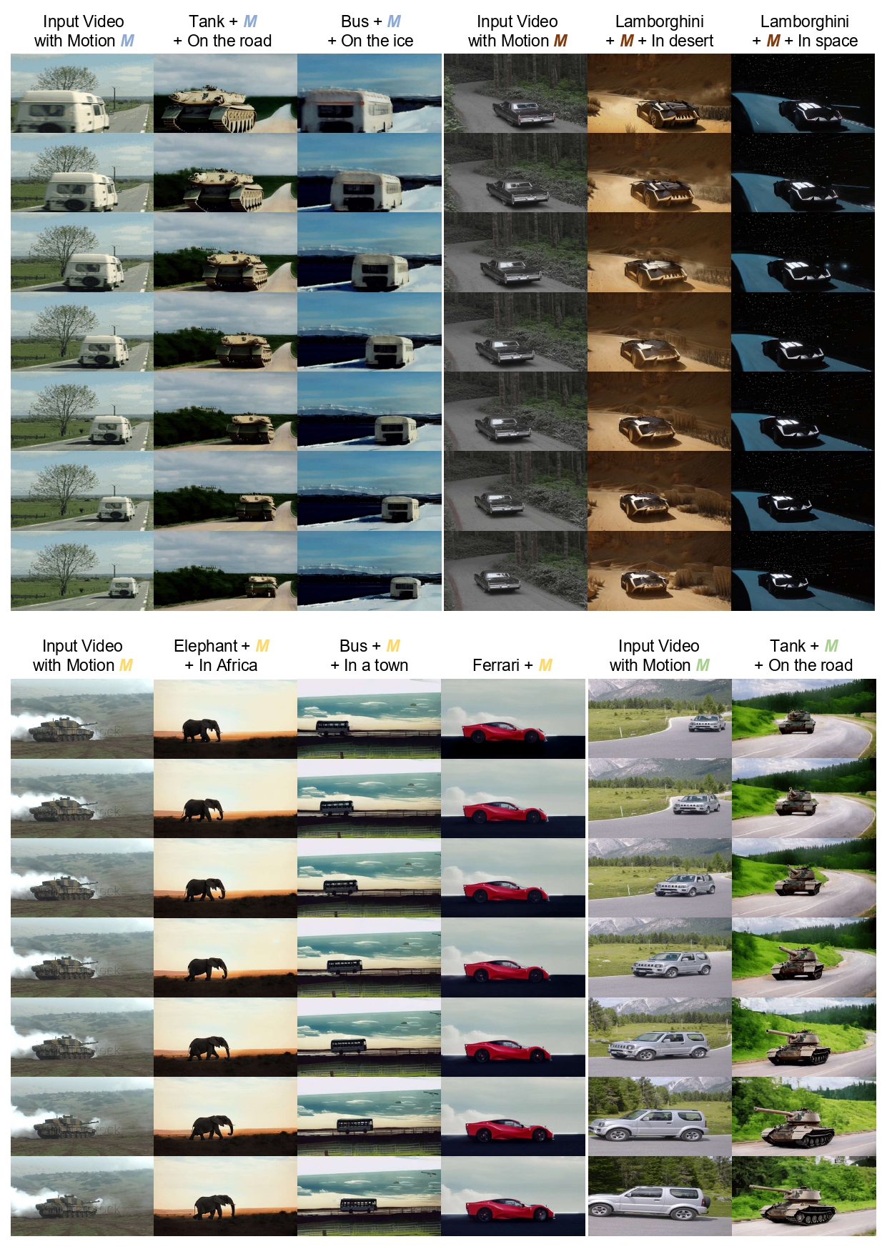
Figure 10: Video Motion Customization results: Keyframes visualized.

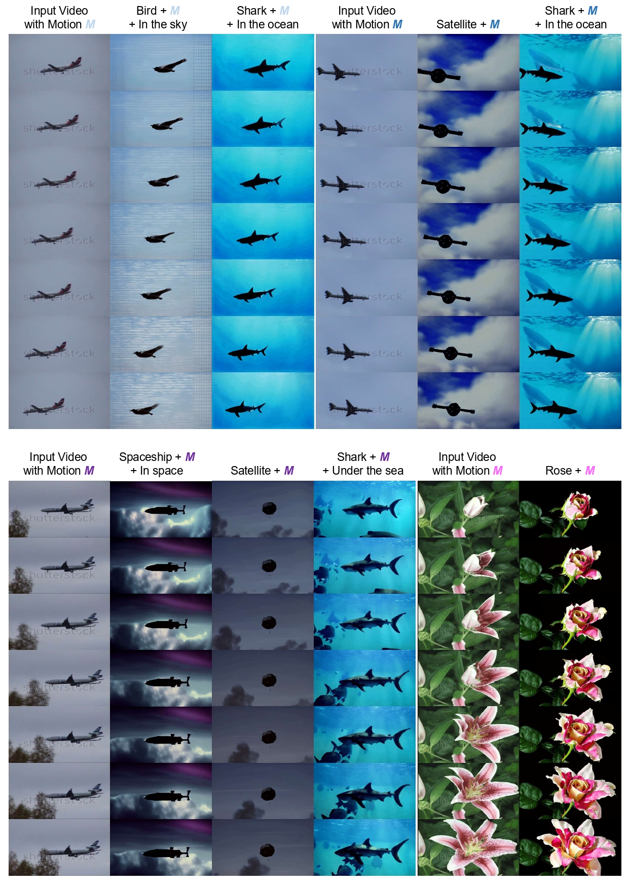
Figure 11: Video Motion Customization results: Keyframes visualized.

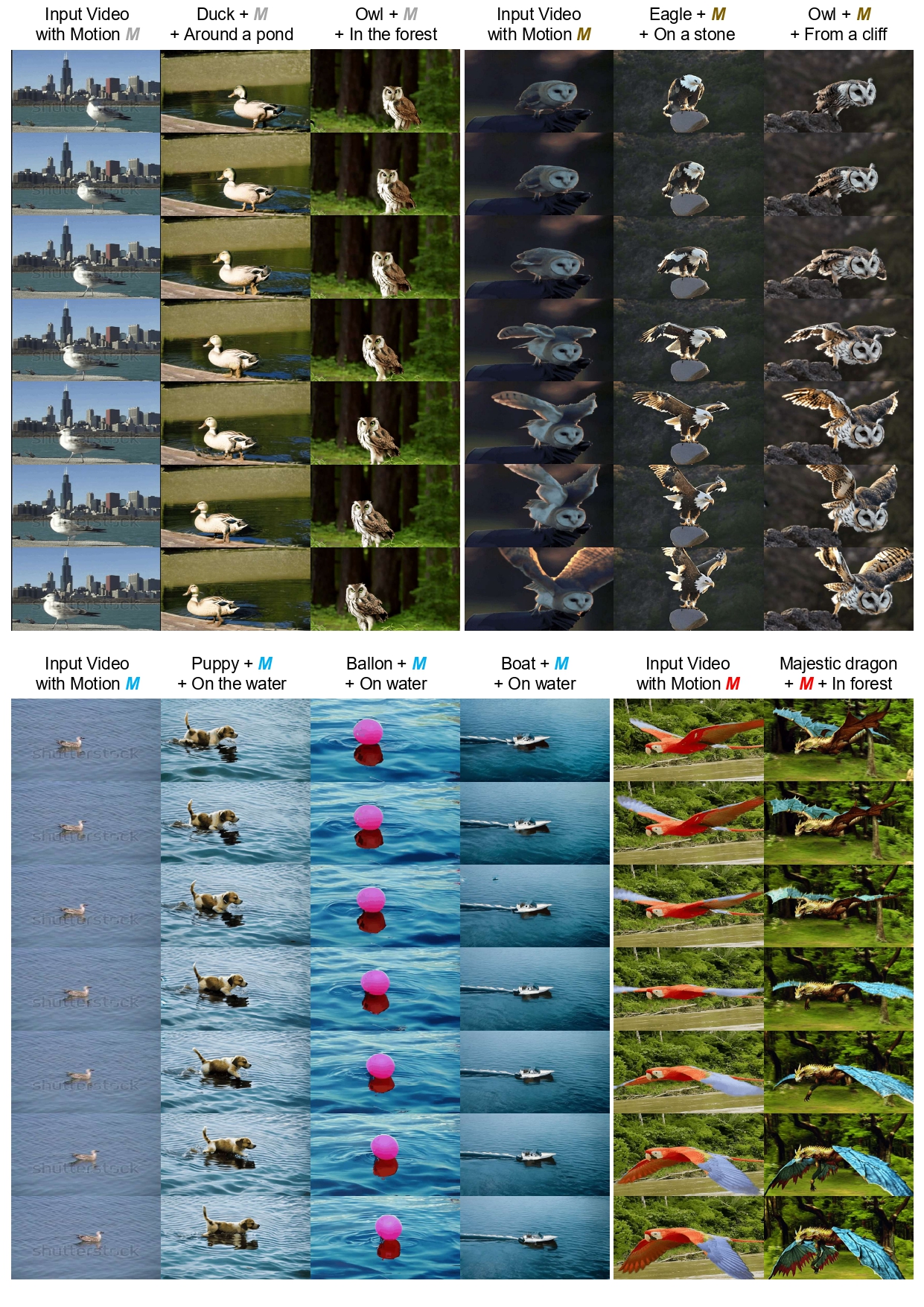
Figure 12: Video Motion Customization results: Keyframes visualized.

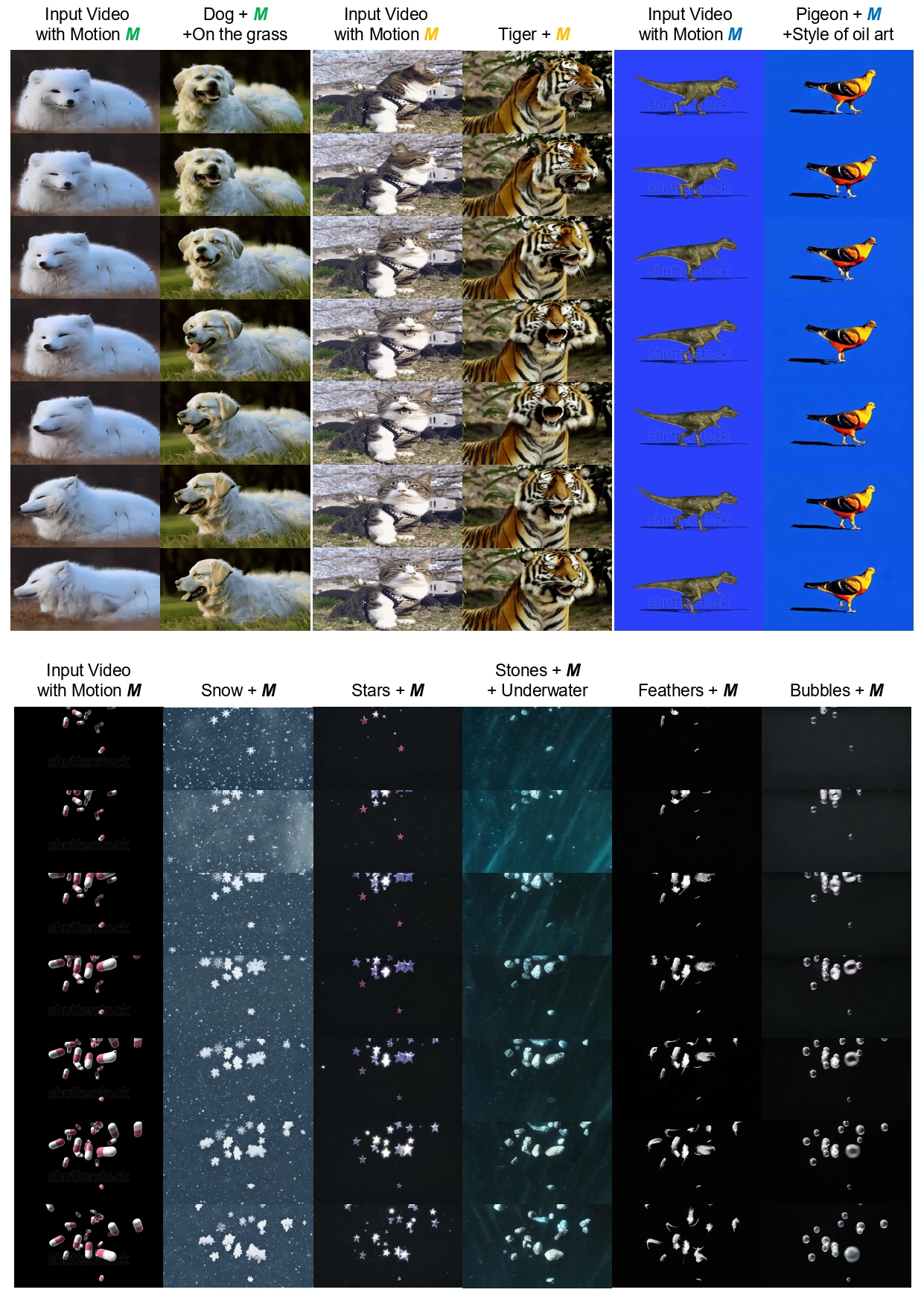
Figure 13: Video Motion Customization results: Keyframes visualized.

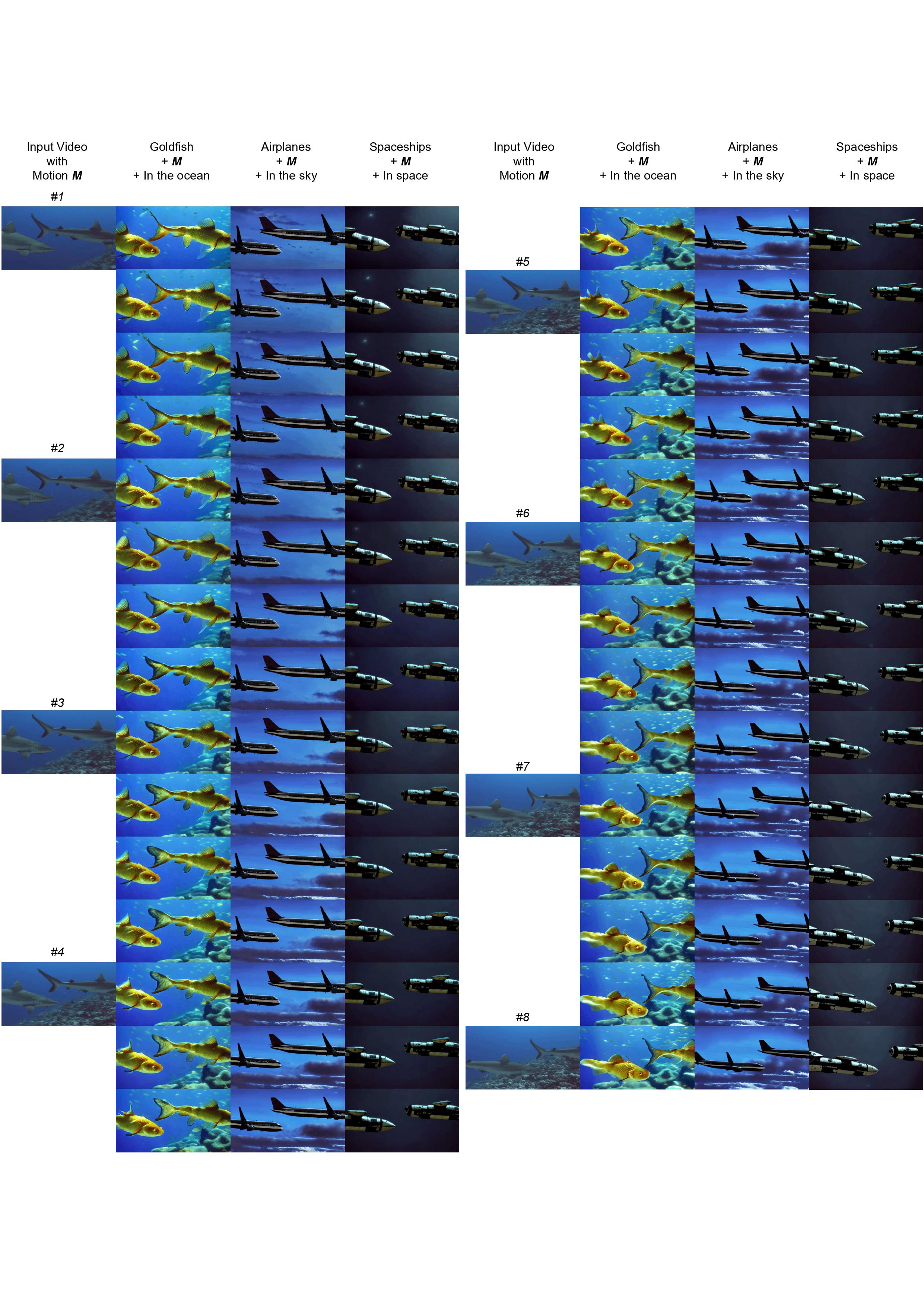
Figure 14: Full-frame results of Video Motion Customization: Text prompt “Sharks are moving” is used for training the keyframe generation UNet.

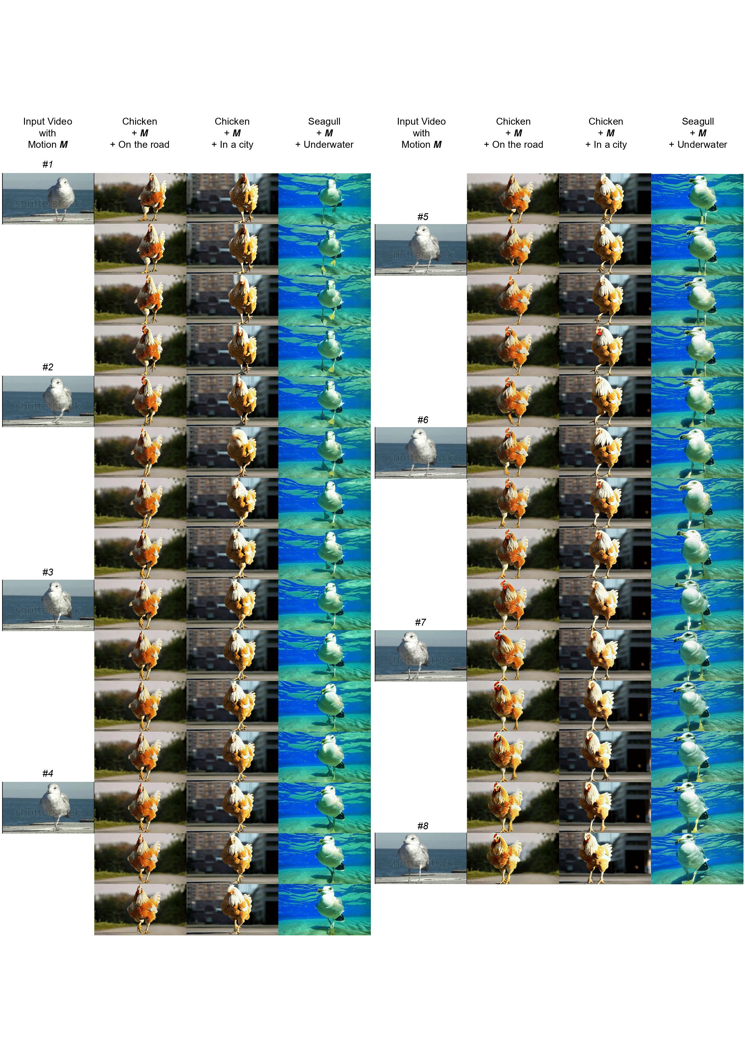
Figure 15: Full-frame results of Video Motion Customization: Text prompt “A seagull is walking” is used for training the keyframe generation UNet.

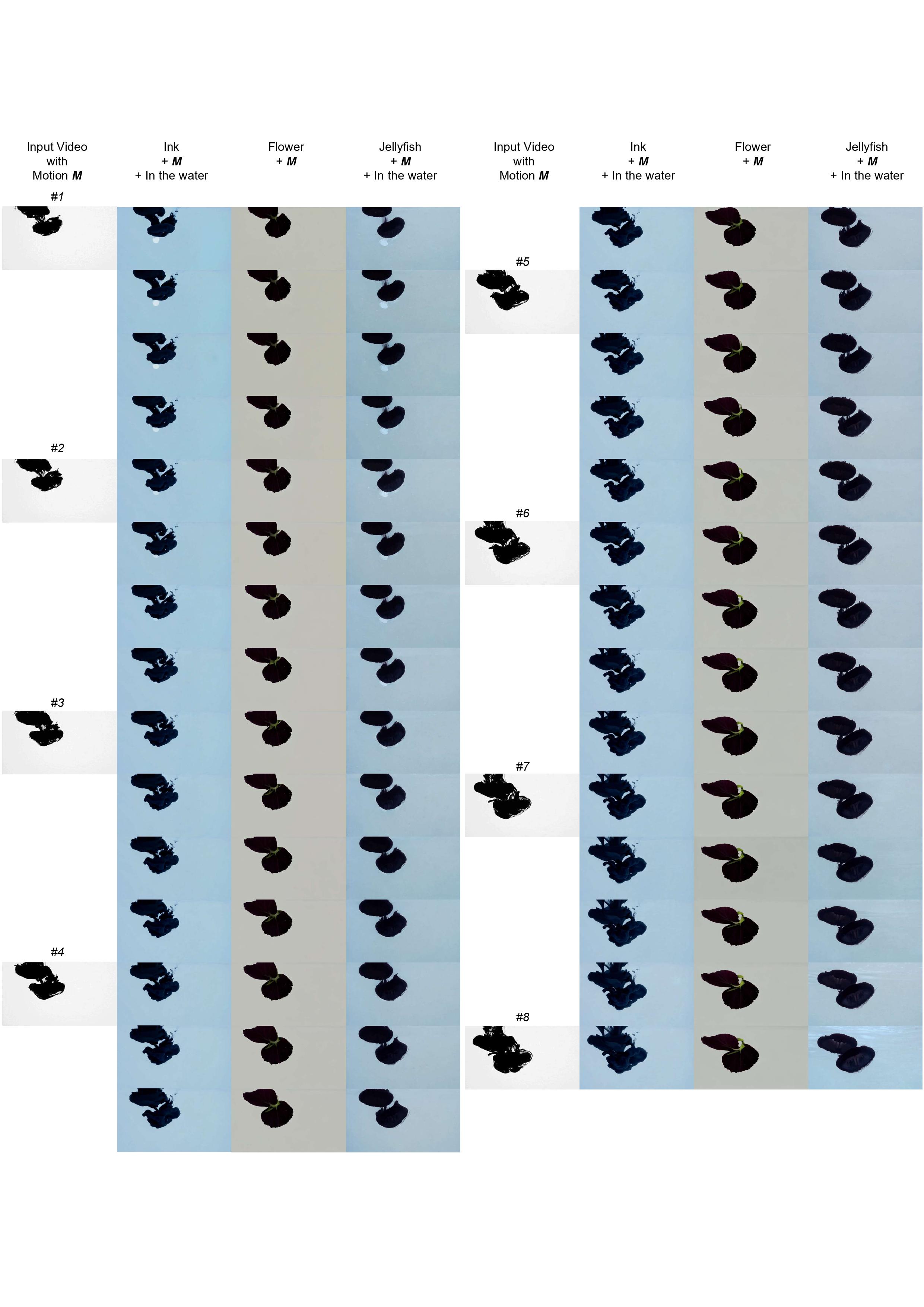
Figure 16: Full-frame results of Video Motion Customization: Text prompt “Ink is spreading” is used for training the keyframe generation UNet.

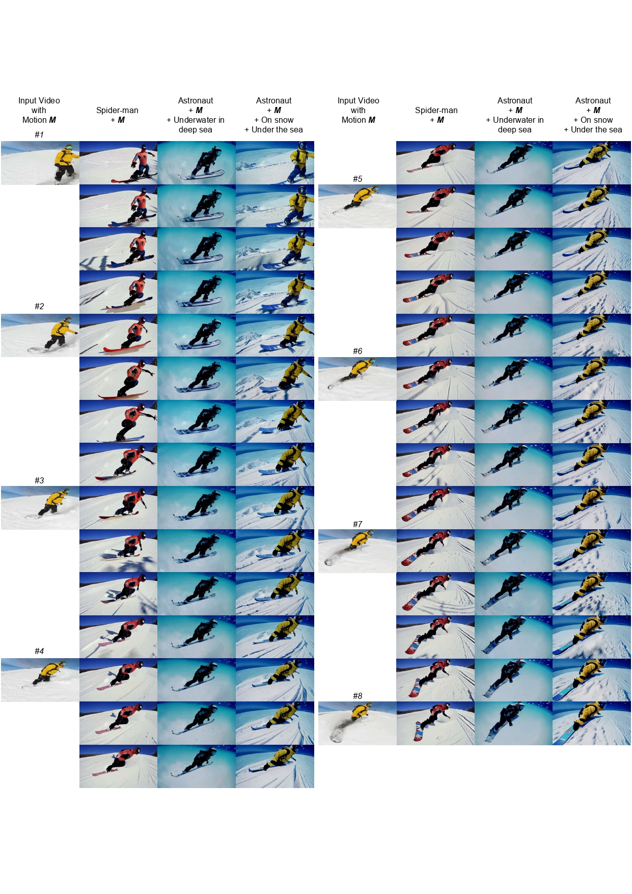
Figure 17: Full-frame results of Video Motion Customization: Text prompt “A man is snowboarding” is used for training the keyframe generation UNet.

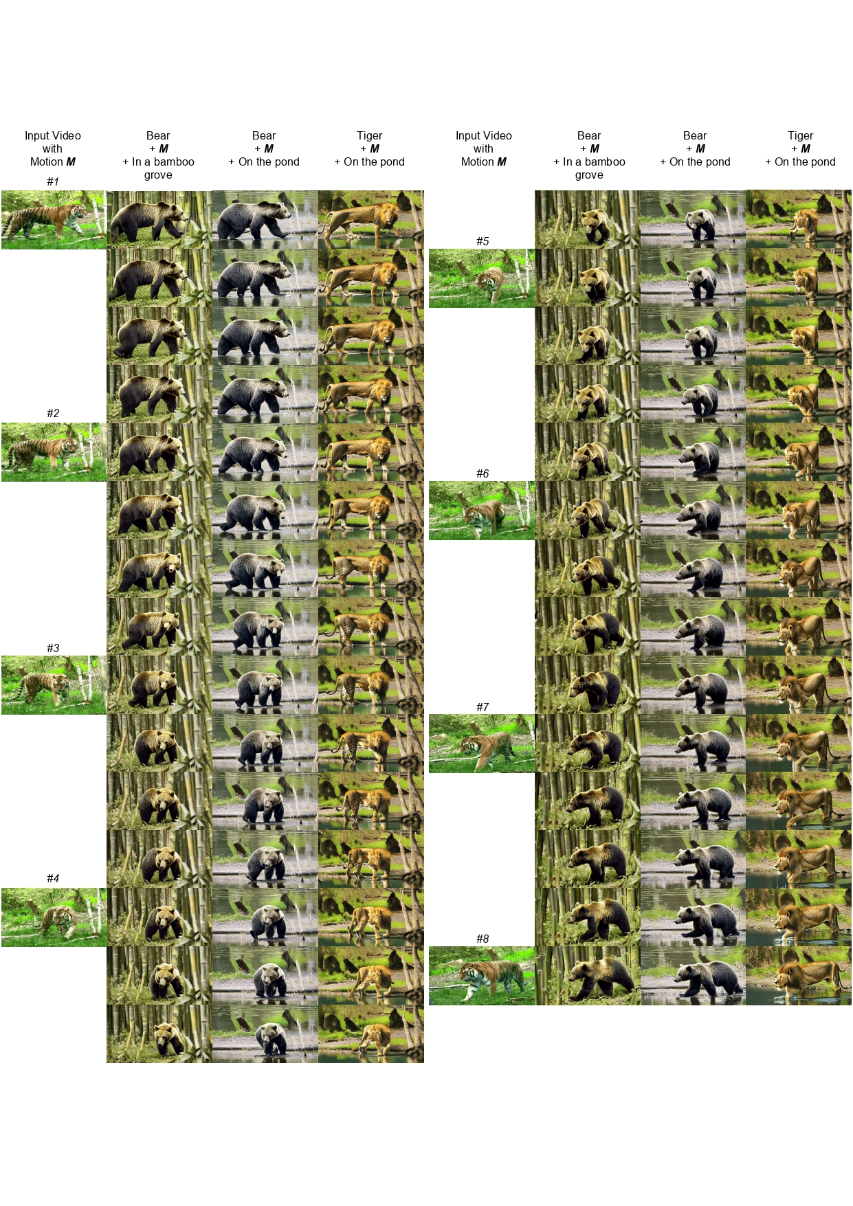
Figure 18: Full-frame results of Video Motion Customization: Text prompt “A tiger is walking” is used for training the keyframe generation UNet.

References

- Bain et al. [2021] Max Bain, Arsha Nagrani, Gül Varol, and Andrew Zisserman. Frozen in time: A joint video and image encoder for end-to-end retrieval. In Proceedings of the IEEE/CVF International Conference on Computer Vision, pages 1728–1738, 2021.
- Blattmann et al. [2023] Andreas Blattmann, Robin Rombach, Huan Ling, Tim Dockhorn, Seung Wook Kim, Sanja Fidler, and Karsten Kreis. Align your latents: High-resolution video synthesis with latent diffusion models. In Proceedings of the IEEE/CVF Conference on Computer Vision and Pattern Recognition, pages 22563–22575, 2023.
- Byeon et al. [2022] Minwoo Byeon, Beomhee Park, Haecheon Kim, Sungjun Lee, Woonhyuk Baek, and Saehoon Kim. Coyo-700m: Image-text pair dataset. https://github.com/kakaobrain/coyo-dataset, 2022.
- Chen et al. [2023a] Hong Chen, Xin Wang, Guanning Zeng, Yipeng Zhang, Yuwei Zhou, Feilin Han, and Wenwu Zhu. Videodreamer: Customized multi-subject text-to-video generation with disen-mix finetuning. arXiv preprint arXiv:2311.00990, 2023a.
- Chen et al. [2023b] Weifeng Chen, Jie Wu, Pan Xie, Hefeng Wu, Jiashi Li, Xin Xia, Xuefeng Xiao, and Liang Lin. Control-a-video: Controllable text-to-video generation with diffusion models. arXiv preprint arXiv:2305.13840, 2023b.
- Efron [2011] Bradley Efron. Tweedie’s formula and selection bias. Journal of the American Statistical Association, 106(496):1602–1614, 2011.
- Esser et al. [2023] Patrick Esser, Johnathan Chiu, Parmida Atighehchian, Jonathan Granskog, and Anastasis Germanidis. Structure and content-guided video synthesis with diffusion models. In Proceedings of the IEEE/CVF International Conference on Computer Vision, pages 7346–7356, 2023.
- Gal et al. [2022] Rinon Gal, Yuval Alaluf, Yuval Atzmon, Or Patashnik, Amit H Bermano, Gal Chechik, and Daniel Cohen-Or. An image is worth one word: Personalizing text-to-image generation using textual inversion. arXiv preprint arXiv:2208.01618, 2022.
- Ge et al. [2023] Songwei Ge, Seungjun Nah, Guilin Liu, Tyler Poon, Andrew Tao, Bryan Catanzaro, David Jacobs, Jia-Bin Huang, Ming-Yu Liu, and Yogesh Balaji. Preserve your own correlation: A noise prior for video diffusion models. In Proceedings of the IEEE/CVF International Conference on Computer Vision, pages 22930–22941, 2023.
- Gu et al. [2023] Yuchao Gu, Xintao Wang, Jay Zhangjie Wu, Yujun Shi, Yunpeng Chen, Zihan Fan, Wuyou Xiao, Rui Zhao, Shuning Chang, Weijia Wu, et al. Mix-of-show: Decentralized low-rank adaptation for multi-concept customization of diffusion models. arXiv preprint arXiv:2305.18292, 2023.
- Han et al. [2023] Ligong Han, Yinxiao Li, Han Zhang, Peyman Milanfar, Dimitris Metaxas, and Feng Yang. Svdiff: Compact parameter space for diffusion fine-tuning. arXiv preprint arXiv:2303.11305, 2023.
- [12] J Ho, T Salimans, A Gritsenko, W Chan, M Norouzi, and DJ Fleet. Video diffusion models. arxiv 2022. arXiv preprint arXiv:2204.03458.
- Ho et al. [2020] Jonathan Ho, Ajay Jain, and Pieter Abbeel. Denoising diffusion probabilistic models. Advances in neural information processing systems, 33:6840–6851, 2020.
- Ho et al. [2022] Jonathan Ho, William Chan, Chitwan Saharia, Jay Whang, Ruiqi Gao, Alexey Gritsenko, Diederik P Kingma, Ben Poole, Mohammad Norouzi, David J Fleet, et al. Imagen video: High definition video generation with diffusion models. arXiv preprint arXiv:2210.02303, 2022.
- Hu et al. [2021] Edward J Hu, Yelong Shen, Phillip Wallis, Zeyuan Allen-Zhu, Yuanzhi Li, Shean Wang, Lu Wang, and Weizhu Chen. Lora: Low-rank adaptation of large language models. arXiv preprint arXiv:2106.09685, 2021.
- Hyvärinen and Dayan [2005] Aapo Hyvärinen and Peter Dayan. Estimation of non-normalized statistical models by score matching. Journal of Machine Learning Research, 6(4), 2005.
- Loshchilov and Hutter [2017] Ilya Loshchilov and Frank Hutter. Decoupled weight decay regularization. arXiv preprint arXiv:1711.05101, 2017.
- Lu et al. [2023] Haoming Lu, Hazarapet Tunanyan, Kai Wang, Shant Navasardyan, Zhangyang Wang, and Humphrey Shi. Specialist diffusion: Plug-and-play sample-efficient fine-tuning of text-to-image diffusion models to learn any unseen style. In Proceedings of the IEEE/CVF Conference on Computer Vision and Pattern Recognition, pages 14267–14276, 2023.
- Ma et al. [2023] Jian Ma, Junhao Liang, Chen Chen, and Haonan Lu. Subject-diffusion: Open domain personalized text-to-image generation without test-time fine-tuning. arXiv preprint arXiv:2307.11410, 2023.
- Micikevicius et al. [2017] Paulius Micikevicius, Sharan Narang, Jonah Alben, Gregory Diamos, Erich Elsen, David Garcia, Boris Ginsburg, Michael Houston, Oleksii Kuchaiev, Ganesh Venkatesh, et al. Mixed precision training. arXiv preprint arXiv:1710.03740, 2017.
- Pont-Tuset et al. [2017] Jordi Pont-Tuset, Federico Perazzi, Sergi Caelles, Pablo Arbeláez, Alex Sorkine-Hornung, and Luc Van Gool. The 2017 davis challenge on video object segmentation. arXiv preprint arXiv:1704.00675, 2017.
- Radford et al. [2021] Alec Radford, Jong Wook Kim, Chris Hallacy, Aditya Ramesh, Gabriel Goh, Sandhini Agarwal, Girish Sastry, Amanda Askell, Pamela Mishkin, Jack Clark, et al. Learning transferable visual models from natural language supervision. In International conference on machine learning, pages 8748–8763. PMLR, 2021.
- Ruiz et al. [2023a] Nataniel Ruiz, Yuanzhen Li, Varun Jampani, Yael Pritch, Michael Rubinstein, and Kfir Aberman. Dreambooth: Fine tuning text-to-image diffusion models for subject-driven generation. In Proceedings of the IEEE/CVF Conference on Computer Vision and Pattern Recognition, pages 22500–22510, 2023a.
- Ruiz et al. [2023b] Nataniel Ruiz, Yuanzhen Li, Varun Jampani, Wei Wei, Tingbo Hou, Yael Pritch, Neal Wadhwa, Michael Rubinstein, and Kfir Aberman. Hyperdreambooth: Hypernetworks for fast personalization of text-to-image models. arXiv preprint arXiv:2307.06949, 2023b.
- Schuhmann et al. [2022] Christoph Schuhmann, Romain Beaumont, Richard Vencu, Cade Gordon, Ross Wightman, Mehdi Cherti, Theo Coombes, Aarush Katta, Clayton Mullis, Mitchell Wortsman, et al. Laion-5b: An open large-scale dataset for training next generation image-text models. Advances in Neural Information Processing Systems, 35:25278–25294, 2022.
- Shi et al. [2023] Jing Shi, Wei Xiong, Zhe Lin, and Hyun Joon Jung. Instantbooth: Personalized text-to-image generation without test-time finetuning. arXiv preprint arXiv:2304.03411, 2023.
- Singer et al. [2022] Uriel Singer, Adam Polyak, Thomas Hayes, Xi Yin, Jie An, Songyang Zhang, Qiyuan Hu, Harry Yang, Oron Ashual, Oran Gafni, et al. Make-a-video: Text-to-video generation without text-video data. arXiv preprint arXiv:2209.14792, 2022.
- Sohl-Dickstein et al. [2015] Jascha Sohl-Dickstein, Eric Weiss, Niru Maheswaranathan, and Surya Ganguli. Deep unsupervised learning using nonequilibrium thermodynamics. In International conference on machine learning, pages 2256–2265. PMLR, 2015.
- Song et al. [2020a] Jiaming Song, Chenlin Meng, and Stefano Ermon. Denoising diffusion implicit models. arXiv preprint arXiv:2010.02502, 2020a.
- Song and Ermon [2019] Yang Song and Stefano Ermon. Generative modeling by estimating gradients of the data distribution. Advances in neural information processing systems, 32, 2019.
- Song et al. [2020b] Yang Song, Jascha Sohl-Dickstein, Diederik P Kingma, Abhishek Kumar, Stefano Ermon, and Ben Poole. Score-based generative modeling through stochastic differential equations. arXiv preprint arXiv:2011.13456, 2020b.
- Wang et al. [2023a] Xiang Wang, Hangjie Yuan, Shiwei Zhang, Dayou Chen, Jiuniu Wang, Yingya Zhang, Yujun Shen, Deli Zhao, and Jingren Zhou. Videocomposer: Compositional video synthesis with motion controllability. arXiv preprint arXiv:2306.02018, 2023a.
- Wang et al. [2023b] Yaohui Wang, Xinyuan Chen, Xin Ma, Shangchen Zhou, Ziqi Huang, Yi Wang, Ceyuan Yang, Yinan He, Jiashuo Yu, Peiqing Yang, et al. Lavie: High-quality video generation with cascaded latent diffusion models. arXiv preprint arXiv:2309.15103, 2023b.
- Wei et al. [2023] Yuxiang Wei, Yabo Zhang, Zhilong Ji, Jinfeng Bai, Lei Zhang, and Wangmeng Zuo. Elite: Encoding visual concepts into textual embeddings for customized text-to-image generation. arXiv preprint arXiv:2302.13848, 2023.
- Wu et al. [2023a] Jay Zhangjie Wu, Yixiao Ge, Xintao Wang, Stan Weixian Lei, Yuchao Gu, Yufei Shi, Wynne Hsu, Ying Shan, Xiaohu Qie, and Mike Zheng Shou. Tune-a-video: One-shot tuning of image diffusion models for text-to-video generation. In Proceedings of the IEEE/CVF International Conference on Computer Vision, pages 7623–7633, 2023a.
- Wu et al. [2023b] Ruiqi Wu, Liangyu Chen, Tong Yang, Chunle Guo, Chongyi Li, and Xiangyu Zhang. Lamp: Learn a motion pattern for few-shot-based video generation. arXiv preprint arXiv:2310.10769, 2023b.
- Zhang et al. [2023] David Junhao Zhang, Jay Zhangjie Wu, Jia-Wei Liu, Rui Zhao, Lingmin Ran, Yuchao Gu, Difei Gao, and Mike Zheng Shou. Show-1: Marrying pixel and latent diffusion models for text-to-video generation. arXiv preprint arXiv:2309.15818, 2023.
- Zhao et al. [2023] Rui Zhao, Yuchao Gu, Jay Zhangjie Wu, David Junhao Zhang, Jiawei Liu, Weijia Wu, Jussi Keppo, and Mike Zheng Shou. Motiondirector: Motion customization of text-to-video diffusion models. arXiv preprint arXiv:2310.08465, 2023.
- Zhou et al. [2022] Daquan Zhou, Weimin Wang, Hanshu Yan, Weiwei Lv, Yizhe Zhu, and Jiashi Feng. Magicvideo: Efficient video generation with latent diffusion models. arXiv preprint arXiv:2211.11018, 2022.