Sparse Beats Dense: Rethinking Supervision in Radar-Camera Depth Completion

Abstract

It is widely believed that the dense supervision is better than the sparse supervision in the field of depth completion, but the underlying reasons for this are rarely discussed. In this paper, we find that the challenge of using sparse supervision for training Radar-Camera depth prediction models is the Projection Transformation Collapse (PTC). The PTC implies that sparse supervision leads the model to learn unexpected collapsed projection transformations between Image/Radar/LiDAR spaces. Building on this insight, we propose a novel “Disruption-Compensation” framework to handle the PTC, thereby relighting the use of sparse supervision in depth completion tasks. The disruption part deliberately discards position correspondences among Image/Radar/LiDAR, while the compensation part leverages 3D spatial and 2D semantic information to compensate for the discarded beneficial position correspondence. Extensive experimental results demonstrate that our framework (sparse supervision) outperforms the state-of-the-art (dense supervision) with 11.6$\%$ improvement in mean absolute error and $1.6\times$ speedup. The code is available at …

1 Introduction

Understanding the three-dimensional (3D) structure of our surrounding scenes can support a variety of spatial tasks, such as perception [49, 50], planning [51, 52], et al. To achieve this, agents typically need to be equipped with multiple sensors, such as cameras, radars to obtain dense depth information. In this paper, we focus on the Radar-Camera depth completion task [11, 12], aiming to obtain a dense and accurate depth map by leveraging image and extremely sparse Radar point clouds (50 to 80 points per frame).

In this field, due to the lack of dense depth ground truth (GT), a single frame of LiDAR is expected to be used as the ground truth for training and testing. However, recent methods [12, 11] have found that training with sparse supervision leads to severe stripe-like scanning pattern artifacts in outputs, as shown in the upper-right section of Fig. 1 (a). The stripe-like scanning pattern artifacts mean that the depth prediction off the supervised points is completely wrong, which is unacceptable for the downstream applications. As a workaround, current methods focus on generating dense supervision data from the sparse data, based on multi-frame stacking or interpolation ways. These approaches inevitably introduce noises such as moving objects, inter-frame noises, interpolation errors, etc. As shown in Fig. 2, in the multi-frame stacked dense supervision of RadarNet [11], there are moving object noises and inter-frame noises. This causes the accuracy of depth completion to drop significantly. For detailed experiments, refer to the supervision ablation experiment of Sec. 5.6.

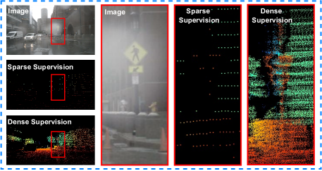
Figure 2: Multi-frame dense supervision is noisy. As shown in the red box, near and far objects are overlapped together due to inter-frame error, which will confuse the depth completion model.

In this paper, we find that models under the sparse supervision tend to learn collapsed projection transformations among the Image-Radar-LiDAR spaces, termed as the Projection Transformation Collapse (PTC). As shown in Fig. 3, the sparse supervision makes models have the same supervision loss value for ideal depth (a) and scan pattern depth (b). The stripe-like artifacts in the output depth map indicate that the model find a bad shortcut, which is position correspondences among Image/Radar/LiDAR spaces, missing the meaningful yet more challenging learning of 3D information. In fact, due to the excessively easily fitting of position correspondences, the model unavoidably learns unexpected collapsed projection transformations. For more details, refer to Sec. 3.

Therefore, based on this key-insight, we design a novel Disruption-Compensation Radar-Camera Depth Completion Framework to handle the PTC. First, the “Disruption” means avoiding the PTC by disrupting the position correspondences among the Image/Radar/LiDAR spaces. Specifically, we decompose the entire disruption process into the 2D Image-LiDAR position correspondences disruption and the 3D Radar-LiDAR position correspondences disruption. For the former, we used spatial augmentation to blur Image-LiDAR position correspondences. For the latter, leveraging the height uncertainty in radar, we disrupt the 3D Radar-LiDAR position correspondences by densifying in the height dimension.

Second, the “Compensation” means compensating for the information lost during the “Disruption” process. Specifically, the “Compensation” consists of two parts: the radar-aware Mask Supervision and the Radar-position Injection Module. The radar-aware mask is a binary mask that indicates the locations of 16 classes in the image, such as cars, people, traffic, etc. Due to radar’s physical characteristics, most response points of 2D radar image are within the radar-aware mask. During training, we use radar-aware mask as an auxiliary supervision, thereby compensating the loss of radar position information. The radar position injection module is a multi-layer perception (MLP) model. It directly extracts information from 3D radar points, guiding the model to fit non-collapsed projection transformations in 3D space, thereby enhancing performance in our task.

Extensive experimental results show that our model accurately predicted the depth of objects in images, successfully outperforming state-of-the-art (SOTA) methods with 11.6$\%$ improvement in mean absolute error, and run $1.6\times$ faster, as shown in Fig. 1 (b). The contributions of the paper are summarized as follows:

• We introduce the Projection Transformation Collapse, which explains why sparse supervision leads to unusable depth maps and is the main challenge in relighting sparse supervision.

• We propose a novel “Disruption-Compensation” framework to address the Projection Transformation Collapse, outperforming other state-of-the-art dense-supervision-based methods in both accuracy and speed.

• We conduct extensive experiments to verify the Projection Transformation Collapse and demonstrate the effectiveness of our framework.

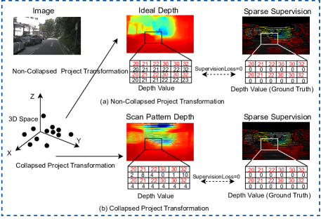
Figure 3: Under the sparse supervision, the ideal depth (a) and the scan pattern depth (b) have the same supervision loss value, shown as the red font in the region-of-interest (ROI) area. In fact, collapsed projection transformation is easier to learn than non-collapsed projection transformation.

2 Related Work

Radar-Camera Depth Completion. Radar-Camera depth completion uses extremely sparse radar point clouds and camera images to obtain dense depth maps with LiDAR point clouds supervision. Existing methods [12, 11] have found that training based on single-frame LiDAR (sparse supervision) leads to severe stripe-like scanning pattern artifacts. As a workaround, previous methods typically employ multi-frame accumulation or interpolation to obtain dense supervision. RadarNet [11] stacks 161 frames of LiDAR data for densification and then removes potentially moving objects (such as cars, people, etc.) based on semantic segmentation masks. RC-PDA [12] uses 25 frames of LiDAR data for stacking and utilizes the optical flow and semantic segmentation masks for occlusion removal. DORN [9] interpolated from sparse LiDAR data and RGB images via the colorization method [26]. While these hand-made “dense” LiDAR supervision methods alleviate the problem, it inevitably introduces noises such as moving objects and inter-frame errors. Even worse, it blurs the projection transformations between the image, radar, and LiDAR coordinate systems. In contrast, our proposed “Disruption-Compensation” framework improves the scanning pattern problem under the sparse supervision and achieves high-performance and efficiency.

LiDAR-Camera Depth Completion. Our task of depth completion has the same goal as LiDAR-Camera depth completion [40, 41, 42, 43, 44, 45, 7]. However, radar point clouds are extremely sparse with low resolution and noisy compared to LiDAR data, which makes these methods unsuitable for this task.

Radar-Camera Object Detection. Radar-Camera depth completion shares a similar goal with detection, which is to fuse complementary information between radar and images [1, 25, 2, 28, 29, 30]. CRAFT [28] associate radar points around the image proposals using adaptive thresholds in polar coordinates. CRN [2] use radar-assisted view transformation (RVT) to transform image and radar features into BEV. However, the above methods aim to force the alignment of radar and image features in 3D space to predict attribute and location of 3D objects. In contrast, Radar-Camera depth completion predicts dense depth under the 2D image plane with sparse supervision, leading to collapsed projection transformation.

Implicit Neural Representation. Implicit neural representation (INR) usually maps the coordinates to visual signal by a multi-layer perceptron (MLP). This is an efficient way to model 3D objects [31, 32, 33], 2D images [16, 14, 13, 34], and 3D scenes [15, 35]. Nerf [15] uses 5D coordinates along camera rays as input to synthesize a novel view. PETR [16] uses a 3D position embedding to encode the 3D position information into 2D features, producing the 3D position-aware features. Inspired by the above methods, we build radar injection module to directly extract information from 3D radar points and guide the model to optimize the projection transformation in 3D spaces.

3 Projection Transformation Collapse

As we analyzed earlier, under the sparse supervision, the supervision loss values generated by non-collapsed and collapsed projection transformations are the same. Consequently, networks are more prone to overfitting to collapsed projection transformations, resulting in stripe-like artifacts on the predicted depth map. However, a question remains: why do networks learn collapsed projection transformations more easily? We find that the position correspondences among Image/Radar/LiDAR play a vital role in this this process.

We hypothesize that, for Radar-Camera depth completion tasks, two types of position correspondences lead to the Projection Transformation Collapse: 2D Image-LiDAR position correspondences and 3D Radar-LiDAR position correspondences. During training, these position correspondences are excessively easy to extract, and as a result, they act like bad “shortcut”, misleading the network to converge to collapsed projection transformation.

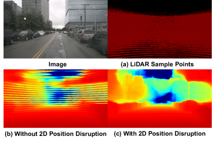
Figure 4: Qualitative comparison between our method with and without the 2D Position Disruption.

3.1 2D Image-to-LiDAR Position Correspondences

Hypothesis 1: 2D Image-LiDAR position correspondences lead to Projection Transformation Collapse. To verify this hypothesis, we use monocular depth prediction model (excluding the influence of radar) to build a comparative experiment.

In Fig. 4 (a), we illustrate the LiDAR sample points at different positions in the 2D LiDAR image. Obviously, there is a 2D Image-Lidar positional correspondence between the image and LiDAR data. In Fig. 4 (b), under the sparse supervision, the monocular depth prediction model also suffer from stripe-like scanning pattern artifacts. Fig. 4 (c) shows that by “disrupting” the 2D Image-Lidar position correspondences through a straightforward ”resize-then-crop” augmentation, the stripe-like scanning pattern artifacts disappear.

Based on the above comparative experiments, it can be concluded that the 2D Image-Lidar position correspondences can cause the Projection Transformation Collapse.

3.2 3D Radar-Lidar Position Correspondences

Hypothesis 2: 3D Radar-Lidar position correspondences lead to Projection Transformation Collapse.  
After confirming the validity of Hypothesis 1, we naturally argue that Hypothesis 2 holds true as well.

Fig. 5 (a) validates this hypothesis. We concatenate the image and 2D radar, feed them into the model, and use the same “position-scale transformation” again. However, the stripe-like artifacts reappear. In Fig. 5 (b), we show a 3D position correspondences disruption operation called “radar-lift”, where we extend the 2D radar points into vertical lines. This method effectively addresses the issue of stripe-like scanning pattern artifacts.

The results of these experiments not only confirm Hypothesis 2 but also emphasize that in Radar-Camera depth completion task, these two types of position correspondences (2D Image-LiDAR and 3D Radar-LiDAR) cause the PTC. It is obviously shown in Fig. 5 (b) that the PTC is resolved.

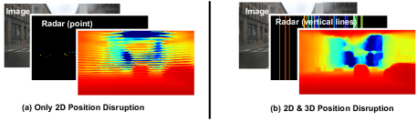
Figure 5: Qualitative comparison between our method with and without the 3D Position Disruption.

4 Method

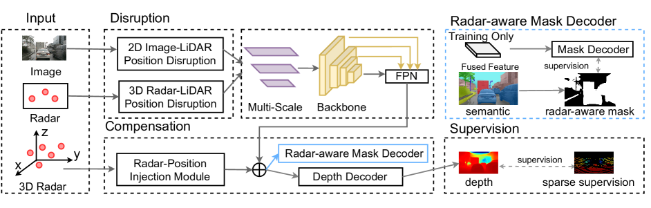
Figure 6: The architecture of “Disruption-Compensation” Radar-Camera Depth Completion Framework. In the Disruption part, the image and radar data are first input into “2D Image-LiDAR Position Disruption” and “3D Radar-LiDAR Position Disruption” respectively, to prevent them from falling into the PTC. In the compensation part, “Radar-Position Injection Module” and “Radar-aware Mask Decoder” are used to compensate for the disrupted corresponding information respectively. Notably, the “Radar-aware Mask Decoder” is a plug-and-play design that is only used during training, requiring no additional computational cost during inference.

Based on the above analysis, we propose a novel “Disruption-Compensation” Radar-Camera depth completion framework to address the Projection Transformation Collapse. The overall architecture of the proposed framework is illustrated in Fig. 6.

In the “Disruption” part, the position correspondences of the“2D Image-LiDAR” and the “3D Radar-LiDAR” are both disrupted to avoid the PTC. In the “Compensation” part, 3D radar points are directly injected into the network through the injection module, while the radar’s potential position is implicitly injected through a radar-aware mask decoder. Notably, the radar-aware mask decoder is a plug-and-play design that is only used during training, requiring no additional computational cost during inference.

4.1 Position Correspondence Disruption

2D Image-Lidar Position Correspondences Disruption. As shown in Fig. 4, there is an obvious position pattern between Image and 2D LiDAR Image. We use a uniform distribution $X\sim U(1,1.5)$ of up-scaling, then crop to the fixed size of $900\times 1600$, for a given image $I\in\mathbb{R}^{3\times H\times W}$ and LiDAR $L\in\mathbb{R}^{\times H\times W}$ pair. This disruption prevents the network from extracting easy-to-fit 2D Image-LiDAR position correspondences.

3D Radar-Lidar Position Correspondences Disruption. Most radars used in automotive vehicles either do not have enough antenna elements along the elevation axis or do not process the radar returns along the elevation axis [11]. Hence, the elevation obtained from them is either too noisy or completely erroneous. Therefore, the 3D Radar-Lidar position correspondence disruption is used to blur the height of points in 2D radar image $I\in\mathbb{R}^{3\times H\times W}$ . For a given 3D radar point $(x,y,z)$, it is first projected onto the 2D image plane $(h,w,d)$, and then expand it to $\{p_{k}=(h_{k},w,d),k=0,1,\dots,H\}$. Thus, any radar point is lifted into vertical line, disrupting the 3D Radar-LiDAR position correspondences.

4.2 Radar-aware Mask Decoder

The Radar-aware Mask Decoder is a plug-and-play module. Its basic idea is that certain objects are more likely to be hit by radar points. Thus, the semantic segmentation regions of these objects, containing potential position information for radar points, can serve as auxiliary supervision during training.

Radar sends electromagnetic (EM) waves [38] through a transmitter. The wave hits objects in the scene, reflects back and is collected by the receiver. Materials that reflect radar signal waves well are those with properties that have minimal absorption of these waves [39], such as metals, aluminum, certain plastics et al. Considering the driving scene, the objects hit by the radar points are more likely to be cars, obstacles, people, traffic lights, walls, etc. This means, in 2D radar image, the majority of radar points are located within the regions of these objects.

Specifically, we select 16 categories of objects in the ADE20K [37] 150 category. Then, we use the union of their semantic segmentation regions to generate the binary radar-aware mask. The Radar-aware Mask Decoder is a type of U-Net decoder, with a single-channel output layer following a sigmoid activation to generate the binary mask. Using radar-aware mask supervision as an auxiliary supervision, we narrow the search space of the points in 2D Radar image by semantic information. In addition to performance gains, the Radar-aware Mask Decoder is designed as a plug-and-play module, avoids extra computational cost during inference.

4.3 Radar Position Injection Module

The Radar Injection Module is a multi-layer perception (MLP) layer, which aims to directly extract positional information of 3D radar points. Given the radar points $\{P_{i}(x_{i},y_{i},z_{i}),i=0,1,\dots n\}$ in the 3D radar coordinates. The radar position injection module of radar points is formulated as:

$$F_{pj}=\Psi(\{P_{i}(x_{i},y_{i},z_{i}),i=0,1,\dots n\})$$ (1)

where $F_{pj}\in\mathbb{R}^{N\times C\times 1\times 1}$ is the position injected feature, and $\Psi$ is a multi-layer perception (MLP) layer. The number of feature map channels in each layer of MLP is (32, 64, 96, 64, 32, 8).

4.4 Depth Completion Network

The deep completion network is a multi-scale U-Net, and its backbone is ResNext [19]. The multi-scale input pyramid, which performs $1/2$ and $1/4$ downsampling on the image and radar respectively, is fed to our network. Specifically, the encoder of U-Net contains 5 layers, and the number of feature map channels output by each layer is (512, 256, 128, 64, 16). At the end of the backbone, there is a feature pyramid network (FPN) [47] for multi-scale feature fusion. A lightweight decoder is used, with the number of channels in each layer being (64, 16, 8, 8, 1).

4.5 Loss Function

The overall loss function is a weighted loss:

$$L=\lambda_{1}L_{G_{1}}+\lambda_{2}L_{G_{2}}+\lambda_{3}L_{G_{3}}$$ (2)

where $\lambda_{1-3}$ is a positive scalar which controls the weights between dense supervised loss at different levels of the pyramid. $G_{1-3}$ represents U-Net networks with different input scales, which are $(1,1/2,1/4)$ respectively.

The used loss function $L_{G_{1-3}}$ is a Smooth L1 loss [48] to increase the robustness of outliers,

$$\textrm{smooth}_{L_{1}}(x)=\begin{cases}0.5x^{2}&\text{if }|x|<1\\ |x|-0.5&\text{otherwise},\end{cases}$$ (3)

Where $x=pred-gt$, only perform sparse supervision at each position with LiDAR.

5 Experiment

Metric	units	Definition
MAE	$mm$	$\frac{1}{|\Omega|}\sum_{x\in\Omega}|\hat{d}(x)-d_{gt}(x)|$
RMSE	$mm$	$(\frac{1}{|\Omega|}\sum_{x\in\Omega}|\hat{d}(x)-d_{gt}(x)|^{2})^{1/2}$

Table 1: Error metrics for evaluating the depth completion bench- marks, where $d_{gt}$ is the ground truth lidar depth map.

Method	GT	Radar Frames	Images	MAE (mm) $\downarrow$			RMSE (mm) $\downarrow$			FPS
				{0-50,70,80m}			{0-50,70,80m}
RC-PDA [12]	25	5	3	2225.0	3326.1	3713.6	4156.5	6700.6	7692.8	11.6
RC-PDA with HG [12]	25	5	3	2315.7	3485.6	3884.3	4321.6	7002.9	8008.6	10.4
DORN [9]	interpolation	5(x3)	1	1926.6	2380.6	2467.7	4124.8	5252.7	5554.3	3.1
R4Dyn [22]	7	4	1	-	-	-	-	-	6434.0	-
Sparse-to-dense [23]	interpolation	3	1	-	-	2374.0	-	-	5628.0	13.2
PnP [24]	interpolation	3	1	-	-	2496.0	-	-	5578.0	9.7
RadarNet [11]	161	1	1	1727.7	2.0732	2179.3	3746.8	4590.7	4898.7	3.7
Ours	1	1	1	1524.5	1822.9	1927.0	3567.3	4303.6	4609.6	21.6

Table 2: Radar-Camera Depth completion on nuScenes, measured in MAE and RMSE (lower is better). Experimental results show that our proposed method outperforms state-of-the-art methods in both accuracy and speed.

5.1 Dataset and Metrics

Dataset. We train and test on the nuScenes [18] dataset. nuScenes is a large-scale multi-modal dataset, which is composed of data from 6 cameras, 1 LiDAR-sensor and 5 radar-sensors. The dataset has 1000 scenes totally and is divided into 700/150/150 scenes as train/validation/test sets, respectively. Refer to RadarNet [11], we utilize pairs of front camera and front radar from nuScenes. Our experiments are conducted using single-frame 2D radar image, without incorporating past or future continuous frame. Additionally, the ground truth for training/testing is a single-frame 2D LiDAR image. The depth range for training and testing is 0-80 meters, with resolutions of inputs and outputs 900 $\times$ 1600.

Metric. We follow the RadarNet [11] metrics. As shown in Tab. 1, We report the Mean Absolute Error (MAE), Root Mean Square Error (RMSE) and test models between 0-50, 0-70 and 0-80 meters.

5.2 Implementation details.

We trained the model using 8 RTX 2080Ti GPUs and tested the speed using 1 A10 GPU on $900\times 1600$ image size. The Adam [20] optimizer was employed with an initial learning rate of 7 $\times 10^{-3}$ and a batch size of 32. We applied a cosine decay strategy for the learning rate scheduling. The total number of training epochs was set to 400. Data augmentation is used during training, including random left-right flipping with a probability of 0.5, and brightness, saturation, and contrast adjustment. All pyramid outputs are supervised, and the corresponding weight hyperparameters are $\lambda_{1}=1$, $\lambda_{2}=0.5$, and $\lambda_{3}=0.25$.

Radar-aware Mask Decoder. ViT-Adapter [36] pre-trained model trained on ADE20K [37] is used to generate semantic segmentation results on nuScenes [18]. We further select 16 categories to generate radar-aware mask, including wall, building, tree, person, car, fence, bus, truck, pole, bicycle, van, minibike.

5.3 State-of-the-Art Comparison

We compare our method against different methods [11, 12, 9, 22, 3, 23, 24] using error metrics Mean Absolute Error (MAE) and Root Mean Square Error (RMSE). Several baselines [12, 22, 3, 23, 24] utilize multiple radar frames or multiple LiDAR frames for depth completion. The multi-frame stacked or interpolated LiDAR will inevitably introduce noise, such as moving objects, or inter-frame errors, etc. In addition, the multi-frame stacked radar input also introduce erroneous guidance depth. RC-PDA [12] even uses multi-frame images for optical flow estimation to obtain more accurate radar and camera alignment. All of the above methods will affect practical application deployment. In contrast, we only use single-frame radar and camera input, with clean single-frame sparse supervision, achieving the SOTA performance and speed.

Results are summarised in Table 2. The number in column ground truth (GT) indicates how many frames of LiDAR are used for densification, while interpolation indicates the use of interpolation algorithms for densification. The “Radar frames” term indicates how many frames of Radar are used for densification, and $\times 3$ indicates that three Radar Sensors are used. To this end, it is noticeable that our method outperformed other baselines on MAE 0-80 meters, e.g., 3713.6 (RC-PDA) vs 2467.7 (DORN) vs 2179.3 (RadarNet) vs 1927.0 (Ours). Our inference speed is the fastest among the above methods, e.g., 11.6 frame-per-second (FPS) (RC-PDA-HG) vs 3.7 FPS (RadarNet) vs 21.7 FPS (Ours). We attribute the efficient inference speed to the single-stage design of our network and, more importantly, the advantages of sparse supervision, enabling the network to be smaller yet perform better.

More qualitative results are shown in Fig. 8. It is obvious that our predicted depth maps have superior visual performance compared to other methods. For instance, in rows 1-2, the scanning pattern of RadarNet is particularly severe in the night environment, making the shape of objects in the scene hard to recognize. The depth map predicted by DORN contains grid artifacts. In addition, our predicted depth map has a more accurate object shape perception, benefiting from the introduction of radar-aware mask decoder. As shown in Fig. 8 rows 2-5, our predicted shapes of people, cars, etc. are more accurate and the car windows are not sliced or adhered to additional objects. In summary, our proposed method achieves better accuracy, speed, and visualization compared to previous methods.

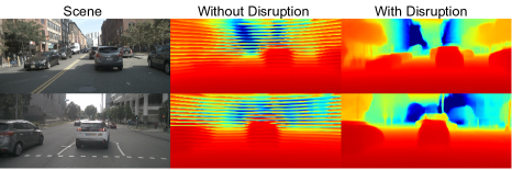
Figure 7: Qualitative comparison between our method with and without “Disruption”. It is obvious that the “Disruption” part of our framework address the Projection Transformation Collapse.

5.4 Ablation Study

We conduct ablations on nuScenes to carefully analyze how much each module contributes to the final performance of our proposed method.

Disruption	Input	MAE 0-80m (mm) $\downarrow$	RMSE 0-80m (mm) $\downarrow$	Scan Pattern
$\times$	Img	3427.4	6411.8	$\times$
$\times$	Img & Radar	1608.3	3376.0	$\checkmark$
$\checkmark$	Img & Radar	2201.1	5103.3	$\times$
$\times$	Img & sparse LiDAR	4646.7	7592.5	$\times$
$\checkmark$	Img & sparse LiDAR	3036.6	6199.4	$\times$

Table 3: Generalization validity of the “Disruption”. Experimental results show that the method without “Disruption” not only outputs scan pattern artifacts, but also has poor generalization performance. When using random sampling sparse LiDAR instead of radar as input, the accuracy is even lower than monocular depth estimation. In contrast, the “Disruption” we proposed improves generalization and achieve artifact-free.

Position Injection	Mask Decoder	MAE 0-80m (mm) $\downarrow$	RMSE 0-80m (mm) $\downarrow$
$\times$	$\times$	2201.1	5103.3
$\checkmark$	$\times$	2116.4	4970.5
$\checkmark$	$\checkmark$	1927.0	4609.6

Table 4: Effectiveness of the “Compensation”. The experiments are all conducted under sparse supervision. The experimental results show that after adding the “Compensation” part, the model restores part of the position correspondence, further improving the accuracy of depth completion.

Effectiveness of “Disruption”. As shown in the Fig. 7, We show a qualitative comparison between our approach with and without “Disruption”. Although this model without “Disruption” is better than baselines, it suffers from stripe-like scanning pattern artifacts, making it challenging to distinguish objects such as cars, people, and buildings etc. This is due to the Projection Transformation Collapse discussed in Sec. 3.

We further conduct experiments to analyze the impact of this Projection Transformation Collapse on generalization. Specifically, we uniformly downsample LiDAR by $60\times$. The number of point clouds in this sparse LiDAR is 50-80 per image, which is similar to radar. Compared to radar point clouds, sparse LiDAR has the advantage of accurate location and noise-free depth. As shown in Tab. 3, after using images and sparse LiDAR as inputs, the accuracy without “Disruption” drops sharply, even lower than the result of monocular depth estimation. On the contrary, after adding our proposed “Disruption”, the generalization ability has been significantly improved, and the qualitative visualization of the depth map has no artifact phenomenon, enabling clear discrimination of object shapes.

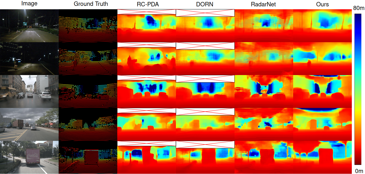
Figure 8: Qualitative results on nuScenes test set (LiDAR best viewed in color at 10x). Since RC-PDA [12] and DORN [9] crop the top sky area for training and inference, we fill the top area with a blank box for comparison. The visualization results show that our proposed “Disruption-Compensation” predict artifact-free depth maps, while scan pattern in RadarNet [11] or the grid phenomenon in DORN [9]. Furthermore, as shown by the truck in row 4-5, our predicted depth map is more accurate for the perception of object shape.

Effectiveness of “Compensation”. Tab. 4 shows the effectiveness of the “Compensation”. It improves the performance by 274.1 mm of MAE (0-80 m) by introducing Radar-Position Injection Module and Radar-aware Mask Decoder. Fig. 8 further illustrates that the “Compensation” part improves accuracy without producing scanning pattern artifacts and falling into the Projection Transformation Collapse. It is worth mentioning that the radar-aware mask decoder in “Compensation” is a plugging design, which improves accuracy without increasing the amount of calculation during inference. This improvement in performance through “Disruption-Compensation” reminds us to rethink the value of sparse supervision, since the sparsity is so common in 3D vision.

Category	Method	MAE 0-80m (mm) $\downarrow$	RMSE 0-80m (mm) $\downarrow$
LiDAR	CompletionFormer [8]	3100.7	6285.8
LiDAR	DySPN [40]	3549.2	6801.9
Radar	ours	1927.0	4609.6

Table 5: Effectiveness of LiDAR-Camera Depth Completion. Experimental results show that directly transferring the depth completion method of LiDAR-Camera to Radar-Camera causes a sharp drop in accuracy and is not suitable for this task.

	Frames	MAE 0-80m (mm) $\downarrow$	RMSE 0-80m (mm) $\downarrow$
RadarNet [11]	161	3104.5	6291.1
DORN [9]	interpolation	2922.3	5895.6
RC-PDA [12]	25	2820.1	6096.6
Disruption-Compensation	1	1927.0	4609.6

Table 6: Experiments with dense supervision. Comparison of different hand-made dense supervision methods on the same Baseline network. The number of Frames represents the number of LiDAR stacked frames, while interpolation represents the use of interpolation algorithms for density. Experimental results show that dense supervision will cause the accuracy to drop sharply.

5.5 LiDAR-Camera Depth Completion

We further reproduce LiDAR-Camera depth completion methods to verify whether it can be directly used for Radar-Camera depth completion, such as CompletionFormer [8], DySPN [40], et al.. As shown in Tab. 5, the direct translation of LiDAR-Camera depth completion to Radar-Camera has low accuracy. This can be attributed to the fact that the height uncertainty and noise of radar point clouds make it difficult to use them like LiDAR. For instance, the LiDAR Camera completion methods tend to directly copy the input point cloud to the output, since the depth obtained by LiDAR is correct, which is different from radar.

5.6 Noisy Dense Supervision

We further conduct experiments to analyze the impact of existing methods, which involve stacking multiple LiDAR frames or interpolation for dense supervision generation. We emphasize here that dense supervision will inevitably introduce noises such as inter-frame noises, interpolation errors, etc. We compare the impact of different dense supervision methods on accuracy, see Tab. 6. RadarNet [11] stacks 161 frames of LiDAR for dense GT, and then removes moving objects based on semantic segmentation. RC-PDA [12] uses 25 frames of LiDAR for stacking and utilizes optical flow and semantic segmentation for occlusion removal. The dense supervision of DORN [9] is interpolated from sparse LiDAR and RGB images via the colorization method [26]. The experimental results show that the depth completion accuracy of the LiDAR after multi-frame stacking decreases as the number of frames increases.

6 Conclusion

It is widely believed that the dense supervision is better than the sparse supervision in the field of depth completion, but the underlying reasons for this are rarely discussed. In this paper, we find that the challenge of the sparse supervision is the unexpected learned collapsed projection transformations between Image/Radar/LiDAR spaces, termed as the Projection Transformation Collapse (PTC). This collapse is due to the model easily learning 2D Image-LiDAR and 3D Radar-LiDAR position correspondences during the training process.

Building on this insight, we design a novel “Disruption-Compensation” Radar-Camera depth completion framework to address of the PTC. The disruption part deliberately discards position correspondences among Image/Radar/LiDAR, while the compensation part leverages 3D spatial and 2D semantic information to compensate for the discarded beneficial information. Extensive experimental results demonstrate that our proposed framework (sparse supervision) outperforms the state-of-the-art (dense supervision) with 11.6$\%$ improvement in mean absolute error and $1.6\times$ speedup.

In summary, we relight the sparse supervision in Radar-Camera depth completion task and demonstrated that accurate sparse supervision outperforms noisy dense supervision. In fact, obtaining accurate and dense supervision is a notoriously challenging task in many fields, such as depth estimation, feature matching, 3D reconstruction, prompting us to rethink the value of sparse supervision. We hope that proposed framework design under the sparse supervision can provide more insights in these fields.

References

- [1] R. Nabati and H. Qi, “Centerfusion: Center-based radar and camera fusion for 3d object detection,” in Proceedings of the IEEE/CVF Winter Conference on Applications of Computer Vision, 2021, pp. 1527–1536.
- [2] Y. Kim, J. Shin, S. Kim, I.-J. Lee, J. W. Choi, and D. Kum, “Crn: Camera radar net for accurate, robust, efficient 3d perception,” in Proceedings of the IEEE/CVF International Conference on Computer Vision, 2023, pp. 17 615–17 626.
- [3] J.-T. Lin, D. Dai, and L. Van Gool, “Depth estimation from monocular images and sparse radar data,” in 2020 IEEE/RSJ International Conference on Intelligent Robots and Systems (IROS). IEEE, 2020, pp. 10 233–10 240.
- [4] T. Wen, Y. Zhang, and N. M. Freris, “Pf-mot: Probability fusion based 3d multi-object tracking for autonomous vehicles,” in 2022 International Conference on Robotics and Automation (ICRA). IEEE, 2022, pp. 700–706.
- [5] S. Imran, Y. Long, X. Liu, and D. Morris, “Depth coefficients for depth completion,” in 2019 IEEE/CVF Conference on Computer Vision and Pattern Recognition (CVPR). IEEE, 2019, pp. 12 438–12 447.
- [6] J. Park, K. Joo, Z. Hu, C.-K. Liu, and I. So Kweon, “Non-local spatial propagation network for depth completion,” in Computer Vision–ECCV 2020: 16th European Conference, Glasgow, UK, August 23–28, 2020, Proceedings, Part XIII 16. Springer, 2020, pp. 120–136.
- [7] S. Imran, X. Liu, and D. Morris, “Depth completion with twin surface extrapolation at occlusion boundaries,” in Proceedings of the IEEE/CVF Conference on Computer Vision and Pattern Recognition, 2021, pp. 2583–2592.
- [8] Y. Zhang, X. Guo, M. Poggi, Z. Zhu, G. Huang, and S. Mattoccia, “Completionformer: Depth completion with convolutions and vision transformers,” in Proceedings of the IEEE/CVF Conference on Computer Vision and Pattern Recognition, 2023, pp. 18 527–18 536.
- [9] C.-C. Lo and P. Vandewalle, “Depth estimation from monocular images and sparse radar using deep ordinal regression network,” in 2021 IEEE International Conference on Image Processing (ICIP). IEEE, 2021, pp. 3343–3347.
- [10] O. Abdulaaty, G. Schroeder, A. Hussein, F. Albers, and T. Bertram, “Real-time depth completion using radar and camera,” in 2022 IEEE International Conference on Vehicular Electronics and Safety (ICVES). IEEE, 2022, pp. 1–6.
- [11] A. D. Singh, Y. Ba, A. Sarker, H. Zhang, A. Kadambi, S. Soatto, M. Srivastava, and A. Wong, “Depth estimation from camera image and mmwave radar point cloud,” in Proceedings of the IEEE/CVF Conference on Computer Vision and Pattern Recognition, 2023, pp. 9275–9285.
- [12] Y. Long, D. Morris, X. Liu, M. Castro, P. Chakravarty, and P. Narayanan, “Radar-camera pixel depth association for depth completion,” in Proceedings of the IEEE/CVF Conference on Computer Vision and Pattern Recognition, 2021, pp. 12 507–12 516.
- [13] X. Hu, H. Mu, X. Zhang, Z. Wang, T. Tan, and J. Sun, “Meta-sr: A magnification-arbitrary network for super-resolution,” in Proceedings of the IEEE/CVF conference on computer vision and pattern recognition, 2019, pp. 1575–1584.
- [14] J. Philion and S. Fidler, “Lift, splat, shoot: Encoding images from arbitrary camera rigs by implicitly unprojecting to 3d,” in Computer Vision–ECCV 2020: 16th European Conference, Glasgow, UK, August 23–28, 2020, Proceedings, Part XIV 16. Springer, 2020, pp. 194–210.
- [15] B. Mildenhall, P. P. Srinivasan, M. Tancik, J. T. Barron, R. Ramamoorthi, and R. Ng, “Nerf: Representing scenes as neural radiance fields for view synthesis,” Communications of the ACM, vol. 65, no. 1, pp. 99–106, 2021.
- [16] Y. Liu, T. Wang, X. Zhang, and J. Sun, “Petr: Position embedding transformation for multi-view 3d object detection,” in European Conference on Computer Vision. Springer, 2022, pp. 531–548.
- [17] C.-C. Lo and P. Vandewalle, “How much depth information can radar contribute to a depth estimation model?” arXiv preprint arXiv:2202.13220, 2022.
- [18] H. Caesar, V. Bankiti, A. H. Lang, S. Vora, V. E. Liong, Q. Xu, A. Krishnan, Y. Pan, G. Baldan, and O. Beijbom, “nuscenes: A multimodal dataset for autonomous driving,” in Proceedings of the IEEE/CVF conference on computer vision and pattern recognition, 2020, pp. 11 621–11 631.
- [19] S. Xie, R. Girshick, P. Dollár, Z. Tu, and K. He, “Aggregated residual transformations for deep neural networks,” in Proceedings of the IEEE conference on computer vision and pattern recognition, 2017, pp. 1492–1500.
- [20] D. P. Kingma and J. Ba, “Adam: A method for stochastic optimization,” in ICLR (Poster), 2015.
- [21] O. Ronneberger, P. Fischer, and T. Brox, “U-net: Convolutional networks for biomedical image segmentation,” in Medical Image Computing and Computer-Assisted Intervention–MICCAI 2015: 18th International Conference, Munich, Germany, October 5-9, 2015, Proceedings, Part III 18. Springer, 2015, pp. 234–241.
- [22] S. Gasperini, P. Koch, V. Dallabetta, N. Navab, B. Busam, and F. Tombari, “R4dyn: Exploring radar for self-supervised monocular depth estimation of dynamic scenes,” in 2021 International Conference on 3D Vision (3DV). IEEE, 2021, pp. 751–760.
- [23] F. Ma and S. Karaman, “Sparse-to-dense: Depth prediction from sparse depth samples and a single image,” in 2018 IEEE international conference on robotics and automation (ICRA). IEEE, 2018, pp. 4796–4803.
- [24] T.-H. Wang, F.-E. Wang, J.-T. Lin, Y.-H. Tsai, W.-C. Chiu, and M. Sun, “Plug-and-play: Improve depth estimation via sparse data propagation,” arXiv preprint arXiv:1812.08350, 2018.
- [25] J.-J. Hwang, H. Kretzschmar, J. Manela, S. Rafferty, N. Armstrong-Crews, T. Chen, and D. Anguelov, “Cramnet: Camera-radar fusion with ray-constrained cross-attention for robust 3d object detection,” in European Conference on Computer Vision. Springer, 2022, pp. 388–405.
- [26] A. Levin, D. Lischinski, and Y. Weiss, “Colorization using optimization,” in ACM SIGGRAPH 2004 Papers, 2004, pp. 689–694.
- [27] G. Brazil, G. Pons-Moll, X. Liu, and B. Schiele, “Kinematic 3d object detection in monocular video,” in Computer Vision–ECCV 2020: 16th European Conference, Glasgow, UK, August 23–28, 2020, Proceedings, Part XXIII 16. Springer, 2020, pp. 135–152.
- [28] Y. Kim, S. Kim, J. W. Choi, and D. Kum, “Craft: Camera-radar 3d object detection with spatio-contextual fusion transformer,” in Proceedings of the AAAI Conference on Artificial Intelligence, vol. 37, no. 1, 2023, pp. 1160–1168.
- [29] Z. Wei, F. Zhang, S. Chang, Y. Liu, H. Wu, and Z. Feng, “Mmwave radar and vision fusion for object detection in autonomous driving: A review,” Sensors, vol. 22, no. 7, p. 2542, 2022.
- [30] D.-H. Paek, S.-H. Kong, and K. T. Wijaya, “K-radar: 4d radar object detection for autonomous driving in various weather conditions,” Advances in Neural Information Processing Systems, vol. 35, pp. 3819–3829, 2022.
- [31] J. J. Park, P. Florence, J. Straub, R. Newcombe, and S. Lovegrove, “Deepsdf: Learning continuous signed distance functions for shape representation,” in Proceedings of the IEEE/CVF conference on computer vision and pattern recognition, 2019, pp. 165–174.
- [32] Z. Chen and H. Zhang, “Learning implicit fields for generative shape modeling,” in Proceedings of the IEEE/CVF Conference on Computer Vision and Pattern Recognition, 2019, pp. 5939–5948.
- [33] L. Mescheder, M. Oechsle, M. Niemeyer, S. Nowozin, and A. Geiger, “Occupancy networks: Learning 3d reconstruction in function space,” in Proceedings of the IEEE/CVF conference on computer vision and pattern recognition, 2019, pp. 4460–4470.
- [34] V. Sitzmann, J. Martel, A. Bergman, D. Lindell, and G. Wetzstein, “Implicit neural representations with periodic activation functions,” Advances in neural information processing systems, vol. 33, pp. 7462–7473, 2020.
- [35] R. Chabra, J. E. Lenssen, E. Ilg, T. Schmidt, J. Straub, S. Lovegrove, and R. Newcombe, “Deep local shapes: Learning local sdf priors for detailed 3d reconstruction,” in Computer Vision–ECCV 2020: 16th European Conference, Glasgow, UK, August 23–28, 2020, Proceedings, Part XXIX 16. Springer, 2020, pp. 608–625.
- [36] Z. Chen, Y. Duan, W. Wang, J. He, T. Lu, J. Dai, and Y. Qiao, “Vision transformer adapter for dense predictions,” arXiv preprint arXiv:2205.08534, 2022.
- [37] B. Zhou, H. Zhao, X. Puig, T. Xiao, S. Fidler, A. Barriuso, and A. Torralba, “Semantic understanding of scenes through the ade20k dataset,” International Journal of Computer Vision, vol. 127, pp. 302–321, 2019.
- [38] M. I. Skolnik, “Introduction to radar systems,” New York, 1980.
- [39] L. Weinstein, “Electromagnetic waves,” Radio i svyaz’, Moscow, 1988.
- [40] Y. Lin, T. Cheng, Q. Zhong, W. Zhou, and H. Yang, “Dynamic spatial propagation network for depth completion,” in Proceedings of the AAAI Conference on Artificial Intelligence, vol. 36, no. 2, 2022, pp. 1638–1646.
- [41] K. Rho, J. Ha, and Y. Kim, “Guideformer: Transformers for image guided depth completion,” in Proceedings of the IEEE/CVF Conference on Computer Vision and Pattern Recognition, 2022, pp. 6250–6259.
- [42] Z. Yan, K. Wang, X. Li, Z. Zhang, J. Li, and J. Yang, “Rignet: Repetitive image guided network for depth completion,” in European Conference on Computer Vision. Springer, 2022, pp. 214–230.
- [43] J. Qiu, Z. Cui, Y. Zhang, X. Zhang, S. Liu, B. Zeng, and M. Pollefeys, “Deeplidar: Deep surface normal guided depth prediction for outdoor scene from sparse lidar data and single color image,” in Proceedings of the IEEE/CVF Conference on Computer Vision and Pattern Recognition, 2019, pp. 3313–3322.
- [44] X. Cheng, P. Wang, and R. Yang, “Depth estimation via affinity learned with convolutional spatial propagation network,” in Proceedings of the European conference on computer vision (ECCV), 2018, pp. 103–119.
- [45] M. Hu, S. Wang, B. Li, S. Ning, L. Fan, and X. Gong, “Penet: Towards precise and efficient image guided depth completion,” in 2021 IEEE International Conference on Robotics and Automation (ICRA). IEEE, 2021, pp. 13 656–13 662.
- [46] Y. Long, D. Morris, X. Liu, M. Castro, P. Chakravarty, and P. Narayanan, “Full-velocity radar returns by radar-camera fusion,” in Proceedings of the IEEE/CVF International Conference on Computer Vision, 2021, pp. 16 198–16 207.
- [47] T.-Y. Lin, P. Dollár, R. Girshick, K. He, B. Hariharan, and S. Belongie, “Feature pyramid networks for object detection,” in Proceedings of the IEEE conference on computer vision and pattern recognition, 2017, pp. 2117–2125.
- [48] R. Girshick, “Fast r-cnn,” in Proceedings of the IEEE international conference on computer vision, 2015, pp. 1440–1448.
- [49] X. Chen, T. Zhang, Y. Wang, Y. Wang, and H. Zhao, “Futr3d: A unified sensor fusion framework for 3d detection,” in Proceedings of the IEEE/CVF Conference on Computer Vision and Pattern Recognition, 2023, pp. 172–181.
- [50] Y. Huang, W. Zheng, Y. Zhang, J. Zhou, and J. Lu, “Tri-perspective view for vision-based 3d semantic occupancy prediction,” in Proceedings of the IEEE/CVF Conference on Computer Vision and Pattern Recognition, 2023, pp. 9223–9232.
- [51] A. Kim, A. Ošep, and L. Leal-Taixé, “Eagermot: 3d multi-object tracking via sensor fusion,” in 2021 IEEE International conference on Robotics and Automation (ICRA). IEEE, 2021, pp. 11 315–11 321.
- [52] A. H. Qureshi, A. Simeonov, M. J. Bency, and M. C. Yip, “Motion planning networks,” in 2019 International Conference on Robotics and Automation (ICRA). IEEE, 2019, pp. 2118–2124.
- [53] V. Patil, C. Sakaridis, A. Liniger, and L. Van Gool, “P3depth: Monocular depth estimation with a piecewise planarity prior,” in Proceedings of the IEEE/CVF Conference on Computer Vision and Pattern Recognition, 2022, pp. 1610–1621.