Ground-state entanglement spectrum of a generic model with nonlocal excitation-phonon coupling

Abstract

While the concept of the entanglement spectrum has heretofore been utilized to address various many-body systems, the models describing an itinerant spinless-fermion excitation coupled to zero-dimensional bosons (e.g. dispersionless phonons) have as yet not received much attention in this regard. To fill this gap, the ground-state entanglement spectrum of a model that includes two of the most common types of short-ranged, nonlocal excitation-phonon interaction – the Peierls- and breathing-mode couplings – is numerically evaluated here. This model displays a sharp, level-crossing transition at a critical coupling strength, which signifies the change from a nondegenerate ground state at the quasimomentum $K_{\textrm{gs}}=0$ to a twofold-degenerate one corresponding to a symmetric pair of nonzero quasimomenta. Another peculiarity of this model is that in the special case of equal Peierls- and breathing-mode coupling strengths the bare-excitation Bloch state with the quasimomentum $0$ or $\pi$ is its exact eigenstate. Moreover, below a critical coupling strength this state is the ground state of the model. Thus, the sharp transition between a bare excitation and a heavily phonon-dressed (polaronic) one can be thought of as a transition between vanishing and finite entanglement. It is demonstrated here that the smallest ground-state entanglement-spectrum eigenvalue to a large extent mimics the behavior of the entanglement entropy itself and vanishes in this special case of the model; by contrast, all the remaining eigenvalues diverge in this case. The implications of excitation-phonon entanglement for $W$-state engineering in superconducting and neutral-atom-based qubit arrays serving as analog simulators of this model are also discussed.

I Introduction

Over the past decade and a half, the concept of the entanglement spectrum established itself as a useful tool for understanding complex patterns of entanglement in strongly-interacting and/or topologically nontrivial quantum many-body systems Laf . Starting from the pioneering work of Li and Haldane Li and Haldane (2008), where this concept was utilized in the context of describing symmetry-protected topological states of matter Fidkowski (2010); Pollmann et al. (2010); Thomale et al. (2010), low-lying entanglement spectra have been employed to glean nontrivial physical insights in many other areas of quantum many-body physics. Examples include, but are not limited to, interacting spin chains Poilblanc (2010); Läuchli and Schliemann (2012); Wu ; Ya , integer quantum Hall effect Schliemann (2011), interacting bosons Den ; Ejima et al. (2014) and fermions Parisen Toldin and Assaad (2018), many-body localization and thermalization in isolated quantum systems Yang et al. (2015); Geraedts et al. (2017), and Floquet dynamical phase transitions Jaf ; Zh ; Lu .

Early attempts to employ quantum information-theoretic tools (e.g. entanglement measures) in the description of many-body systems pertained to the use of entanglement entropy to characterize various quantum phase transitions Ami . The entanglement entropy Weh ; Hayashi (2017) of a quantum system that can be partitioned into two entangled subsystems (a bipartite quantum system) is given by the von Neumann entropy of the reduced density matrix corresponding to either one of the two subsystems (obtained by tracing out the other subsystem) Laf . While this quantity does represent a measure of entanglement in any given state of such a system, the full entanglement spectrum – i.e., the spectrum of the negative logarithm of the reduced density matrix Chandran et al. (2014) – yields a much more detailed characterization of the entanglement in the system.

This paper is focussed on the ground-state entanglement spectrum of a one-dimensional (1D) lattice model describing an itinerant spinless-fermion excitation coupled to zero-dimensional bosons (e.g., dispersionless phonons) through two different short-ranged coupling mechanisms. The entanglement aspects of coupled excitation-phonon (e-ph) models – not least those pertaining to entanglement spectra – have heretofore not been given due attention Sto (c); Roo . While the dearth of entanglement-related studies of such models is the primary motivation behind the present work, the choice of e-ph interaction mechanisms to be discussed here – namely, Peierls (P) and breathing-mode (BM) type couplings – is motivated by their relevance in various physical systems.

Models with short-ranged e-ph coupling describe the interaction of an excess charge carrier (or an exciton) in certain classes of electronic materials (e.g., narrow-band semiconductors) with optical phonons of the host crystal Han ; Hannewald et al. (2004); Rösch et al. (2005); Sle ; Vukm ; Stogra ; Vuk (b); Shn (a, b). In the extreme case of strong e-ph coupling, a heavily phonon-dressed excitation is formed (small polaron) Ran ; Alexandrov and Devreese (2010). While the bulk of small-polaron-related studies Ranninger and Thibblin (1992); Capone et al. (1997); Wel ; Jeckelmann and White (1998); Bonča et al. (1999); Zoli (2003); Stojanović et al. (2004, 2012); Mei et al. (2013); Chakraborty et al. (2016); Jan have so far been carried out within the framework of the Holstein model Holstein (1959), which accounts for the purely local e-ph coupling, over the past two decades considerable attention was devoted to nonlocal-coupling mechanisms Zoli (2003); Stojanović et al. (2004). The most well-known among them is P-type coupling Stojanović et al. (2004); Stojanović and Vanević (2008), which is manifested through the dependence of the dynamically-fluctuating excitation hopping amplitude between two adjacent lattice sites on the difference of Einstein-phonon displacements on those sites. On the other hand, BM-type coupling accounts for a change in the on-site energy of an itinerant excitation due to phonon displacements on the two adjacent sites; being also of the density-displacement type, it can be viewed as a nonlocal counterpart of Holstein-type coupling.

What makes strongly momentum-dependent e-ph interactions – those like P-type coupling, whose vertex function depends both on the excitation- and phonon quasimomenta – particularly interesting is the fact that they allow the possibility of sharp, level-crossing transitions at a critical e-ph coupling strength; according to the Gerlach-Löwen theorem Ger (a, b), transitions of this type are forbidden for momentum-independent (Holstein-type) coupling and those that depend on the phonon quasimomentum, but not on that of the excitation (e.g., Fröhlich-type coupling Fro ). Such a sharp transition corresponds to a change from a nondegenerate ground state at the quasimomentum $K_{\textrm{gs}}=0$ to a twofold-degenerate one corresponding to a pair of equal and opposite (nonzero) quasimomenta. It was already demonstrated such transitions take place in a model with P-type coupling Stojanović and Vanević (2008), as well as in its counterpart with simultaneous P and BM couplings discussed in the present work Stojanović et al. (2014); Stojanović and Salom (2019).

Aside from the occurrence of a sharp ground-state transition, another peculiar feature of the model under consideration – with simultaneous P and BM couplings – is that in the special case when the two coupling strengths are equal the bare-excitation Bloch state with the quasimomentum $k=0$ (or $k=\pi$) is its eigenstate. Furthermore, below a critical coupling strength this bare-excitation state – with no e-ph entanglement – represents the ground state of the model. In the two existing proposals for the physical realization of this model – with superconducting qubits coupled to resonators Stojanović et al. (2014); Stojanović and Salom (2019); Nau and neutral-atom-based Sto (d) Rydberg-dressed qubit arrays – this feature translates into the possibility of engineering $W$-type states Sto (d, a), maximally-entangled multiqubit states of interest for quantum-technology applications.

Here the ground-state entanglement spectrum of a model with simultaneous P and BM couplings is studied in a numerically-exact fashion, the primary aim of this study being to describe the dependence of this spectrum on the effective e-ph coupling strength. In addition to verifying that each entanglement-spectrum eigenvalue undergoes nonanalyticities at critical coupling strengths, it is demonstrated here that the entanglement entropy around this transition point is predominantly determined by the smallest eigenvalue. This eigenvalue to a large extent mimics the behavior of the entropy and vanishes in the special case of equal P and BM coupling strengths; at the same time, all the remaining entanglement-spectrum eigenvalues diverge for equal coupling strengths, while still yielding vanishing contributions to the entanglement entropy. The implications of the behavior of the entanglement spectrum and the corresponding entropy in the latter case for the generation of $W$ states in the previously proposed analog quantum simulators of the model under consideration are also discussed.

This article is organized as follows. In Sec. II the coupled e-ph Hamiltonian – comprising P- and BM coupling terms – is introduced, along with a discussion of the bare-excitation eigenstates in a special case of this model and a short description of possible physical realizations of this model. Section III starts with a short recapitulation of the definition and general properties of entanglement spectra, followed by the essential details of their application in the coupled e-ph system under consideration. Some mathematical consequences of the discrete translational symmetry of the system, as well as the relevant details of the truncation of the total Hilbert space of the system, are discussed in Sec. IV. The principal results of the paper are presented and discussed in Sec. V. To end with, the paper is summarized in Sec. VI. In order not to interrupt the main flow of the paper, some mathematical derivations are relegated to Appendices A and B.

II Model

To set the stage for further discussion, the coupled e-ph Hamiltonian with Peierls- and breathing-mode coupling terms is introduced, both in the real-space (lattice) and momentum-space representations (Sec. II.1). An interesting special case of this Hamiltonian – namely, the one with equal coupling strengths for the two relevant e-ph interaction mechanisms – is then briefly discussed (Sec. II.2). For the sake of completeness, this is followed by a short description of two proposed physical realizations of the model under consideration (Sec. II.3).

II.1 Hamiltonian and its ground-state properties

The 1D lattice model under consideration describes a single spinless-fermion excitation interacting with dispersionless (Einstein-type) phonons through two different nonlocal e-ph coupling mechanisms. The Hamiltonian of this model is given by $H=H_{0}+H_{\textrm{e-ph}}$, where $H_{0}$ is the noninteracting and $H_{\textrm{e-ph}}$ the interacting (e-ph) part. The noninteracting part $H_{0}$ consists of the excitation kinetic-energy term, with the corresponding hopping amplitude $t_{\textrm{e}}$, and free-phonon terms ($\hbar=1$):

$$H_{0}=-t_{\textrm{e}}\sum_{n}(c^{\dagger}_{n+1}c_{n}+\mathrm{H.c.})+\omega_{\textrm{ph}}\sum_{n}a^{\dagger}_{n}a_{n}\>.$$ (1)

Here $c^{\dagger}_{n}$ ($c_{n}$) creates (annihilates) an excitation at site $n$ ($n=1,\ldots,N$) of the underlying 1D lattice, while $a^{\dagger}_{n}$ ($a_{n}$) creates (annihilates) a zero-dimensional (Einstein) phonon with frequency $\omega_{\textrm{ph}}$ at the same site.

The total e-ph coupling part $H_{\textrm{e-ph}}$ of the total Hamiltonian consists of the Peierls- (P) and breathing-mode (BM) contributions. The P contribution Stojanović et al. (2004); Stojanović and Vanević (2008) accounts for the linear dependence of the effective (dynamically dependent on the phonon degrees of freedom) excitation-hopping amplitude between sites $n$ and $n+1$ on the difference of the respective local phonon displacements. In its most succinct form, it is given by

$$H_{\textrm{P}}=g_{\textrm{P}}\omega_{\textrm{ph}}\>l_{0}^{-1}\>\sum_{n}(c_{n}^{\dagger}c_{n+1}+\textrm{H.c.})\>(u_{n+1}-u_{n})\>,$$ (2)

where $g_{\textrm{P}}$ is the corresponding dimensionless P-coupling strength and $u_{n}\equiv l_{0}(a_{n}+a_{n}^{\dagger})$ the phonon displacement at site $n$, with $l_{0}$ being the phonon zero-point length. At the same time, the BM contribution captures the antisymmetric nonlocal coupling of the excitation density at site $n$ with the local phonon displacements on the nearest-neighbor sites $n\pm 1$ Sle ; Stojanović et al. (2014). This density-displacement type coupling term is given by

$$H_{\textrm{BM}}=g_{\textrm{BM}}\omega_{\textrm{ph}}\>l_{0}^{-1}\>\sum_{n}c_{n}^{\dagger}c_{n}(u_{n-1}-u_{n+1})\>,$$ (3)

where $g_{\textrm{BM}}$ stands for the dimensionless BM-coupling strength. In their most explicit forms, the coupling terms $H_{\textrm{P}}$ and $H_{\textrm{BM}}$ are given by [cf. Eqs. (2) and (3)]

$$H_{\textrm{P}} = g_{\textrm{P}}\omega_{\textrm{ph}}\sum_{n}(c^{\dagger}_{n+1}c_{n}+\mathrm{H.c.})$$ (4)

$$\times (a^{\dagger}_{n+1}+a_{n+1}-a^{\dagger}_{n}-a_{n})\>,$$

$$H_{\textrm{BM}} = g_{\textrm{BM}}\omega_{\textrm{ph}}\sum_{n}c^{\dagger}_{n}c_{n}$$

$$\times (a^{\dagger}_{n-1}+a_{n-1}-a^{\dagger}_{n+1}-a_{n+1})\>.$$

The total e-ph coupling Hamiltonian $H_{\textrm{e-ph}}=H_{\textrm{P}}+H_{\textrm{BM}}$ can be recast in the generic momentum-space form

$$H_{\textrm{e-ph}}=\frac{1}{\sqrt{N}}\sum_{k,q}\gamma_{\textrm{e-ph}}(k,q)\>c_{k+q}^{\dagger}c_{k}(a_{-q}^{\dagger}+a_{q})\>,$$ (5)

where the P- and BM contributions to the total e-ph vertex function $\gamma_{\textrm{e-ph}}(k,q)=\gamma_{\textrm{P}}(k,q)+\gamma_{\textrm{BM}}(q)$ are given by

$$\gamma_{\textrm{P}}(k,q) = 2ig_{\textrm{P}}\>\omega_{\textrm{ph}}\>[\sin k-\sin(k+q)]\>,$$ (6)

$$\gamma_{\textrm{BM}}(q) = 2ig_{\textrm{BM}}\>\omega_{\textrm{ph}}\>\sin q\>.$$ (7)

[Note that quasimomenta $k$ and $q$ in Eqs. (6) and (7) are assumed to be dimensionless, i.e., expressed in units of the inverse lattice period; this convention will be used throughout the remainder of this paper.]

For the most general ($k$- and $q$-dependent) vertex function $\gamma_{\textrm{e-ph}}(k,q)$, the effective coupling strength is given by

$$\lambda_{\textrm{e-ph}}=\frac{\langle|\gamma_{\textrm{e-ph}}(k,q)|^{2}\rangle_{\textrm{BZ}}}{2t_{\rm e}\>\omega_{\textrm{ph}}}\>,$$ (8)

where $\langle\ldots\rangle_{\textrm{BZ}}$ is the Brillouin-zone (BZ) average over the quasimomenta $k,q\in(-\pi,\pi]$. A straightforward derivation (for details, see Appendix A) leads to the following results for the effective P- and BM coupling strengths:

$$\lambda_{\textrm{P}}=2g^{2}_{\textrm{P}}\>\frac{\omega_{\textrm{ph}}}{t_{\rm e}}\qquad,\qquad\lambda_{\textrm{BM}}=g^{2}_{\textrm{BM}}\>\frac{\omega_{\textrm{ph}}}{t_{\rm e}}\>.$$ (9)

It is also important to notice that – due to the specific momentum dependence of the two relevant (P and BM) e-ph couplings [cf. Eqs. (6) and (7)] – the total effective e-ph coupling strength $\lambda_{\textrm{e-ph}}$ [cf. Eq. (8)] is given by the sum of $\lambda_{\textrm{P}}$ and $\lambda_{\textrm{BM}}$, i.e. $\lambda_{\textrm{e-ph}}=\lambda_{\textrm{P}}+\lambda_{\textrm{BM}}$ (for details, see again Appendix A).

It is worthwhile pointing out that – as a direct implication of the discrete translational symmetry of the system (regardless of the concrete form of $H_{\textrm{e-ph}}$) – the eigenstates of the total Hamiltonian $H=H_{0}+H_{\textrm{e-ph}}$ ought to be good-quasimomentum states. More precisely, these states – the Bloch eigenstates of the coupled e-ph system at hand – are the joint eigenstates of the total Hamiltonian $H$ and the total quasimomentum operator

$$K_{\textrm{tot}}=\sum_{k}k\>c^{\dagger}_{k}c_{k}+\sum_{q}q\>a^{\dagger}_{q}a_{q}\>,$$ (10)

because the latter commutes with $H$. In the following, the eigenvalues of $K_{\textrm{tot}}$ will be labelled by $K\in(-\pi.\pi]$.

The fact that the total e-ph vertex function in Eq. (5) depends on both the excitation ($k$) and phonon ($q$) quasimomenta implies that the Hamiltonian $H_{\textrm{e-ph}}$ does not satisfy the conditions for the applicability of the Gerlach-Löwen theorem, which rules out the existence of nonanalyticites in the ground-state-related quantities Ger (b). In particular, the ground state of the total Hamiltonian $H=H_{0}+H_{\textrm{e-ph}}$ under consideration undergoes a sharp, level-crossing-type transition at a certain non-universal (i.e., dependent on the adiabaticity ratio $\omega_{\textrm{ph}}/t_{\rm e}$) critical value $\lambda^{\textrm{c}}_{\textrm{e-ph}}\sim 1$ of the effective coupling strength Stojanović and Vanević (2008). Below this critical value (i.e. for $\lambda_{\textrm{e-ph}}<\lambda^{\textrm{c}}_{\textrm{e-ph}}$) the ground state is nondegenerate and represents the $K=0$ eigenvalue of $K_{\mathrm{tot}}$; on the other hand, for $\lambda_{\textrm{e-ph}}\geq\lambda^{\textrm{c}}_{\textrm{e-ph}}$ the ground state is twofold-degenerate and corresponds to a pair of equal- and opposite (nonzero) quasimomenta. With $\lambda_{\textrm{e-ph}}$ increasing beyond its critical value (corresponding to the given value of the adiabaticity ratio), the pair of quasimomenta $K_{\textrm{gs}}$ that corresponds to the twofold-degenerate ground state also varies; this is reflected in the ground-state energy undergoing a sequence of further first-order nonanalyticities. Finally, this quasimomentum saturates at $K_{\textrm{gs}}=\pm\pi/2$ for $\lambda_{\textrm{e-ph}}$ above a threshold value; the latter also depends on $\omega_{\textrm{ph}}/t_{\rm e}$ and is larger than the corresponding $\lambda^{\textrm{c}}_{\textrm{e-ph}}$.

II.2 Bare-excitation Bloch eigenstates for $g_{\textrm{P}}=g_{\textrm{BM}}$

The model under consideration has an interesting property in the special case when the two relevant coupling strenghts are the same (i.e., $g_{\textrm{P}}=g_{\textrm{BM}}$). Namely, in this special case the coupled e-ph Hamiltonian of the system posseses a bare-excitation Bloch eigenstate for an arbitrary e-ph coupling strength. This eigenstate $|\Psi_{k}\rangle\equiv c^{\dagger}_{k}|0\rangle_{\textrm{e}}\otimes|0\rangle_{\textrm{ph}}$ (where $|0\rangle_{\textrm{e}}$ and $|0\rangle_{\textrm{ph}}$ are the excitation and phonon vacuum states, respectively) corresponds to the excitation quasimomentum $k=0$ in the case of positive hopping amplitude ($t_{e}>0$), while for $t_{e}<0$ it corresponds to $k=\pi$.

It is rather straightforward to show that $|\Psi_{k=0}\rangle\equiv c^{\dagger}_{k=0}|0\rangle_{\textrm{e}}\otimes|0\rangle_{\textrm{ph}}$ is an eigenstate of the total Hamiltonian for ($t_{e}>0$) (the proof that $|\Psi_{k=\pi}\rangle$ is its eigenstate for $t_{e}<0$ is completely analogous). Namely, because $|\Psi_{k=0}\rangle$ is an eigenstate of the noninteracting part $H_{0}$ of the system Hamiltonian (for $t_{e}>0$), to demonstrate that it is also an eigenstate of $H$ it is sufficient to prove that this state is simultaneously an eigenstate of $H_{\textrm{e-ph}}$ [cf. Eq. (5)]. By acting with $H_{\textrm{e-ph}}$ on $|\Psi_{k=0}\rangle$, taking into account that $c_{k}c_{k=0}^{\dagger}\>|0\rangle_{\textrm{e}}\equiv\delta_{k,0}|0\rangle_{\textrm{e}}$, one readily finds that

$$H_{\textrm{e-ph}}|\Psi_{k=0}\rangle=\frac{1}{\sqrt{N}}\sum_{q}\gamma_{\textrm{e-ph}}(k=0,q)\>c_{q}^{\dagger}|0\rangle_{\textrm{e}}\otimes a_{-q}^{\dagger}|0\rangle_{\textrm{ph}}\>.$$ (11)

Given that for the vertex functions in Eqs. (5)–(7) it holds that (for an arbitrary phonon quasimomentum $q$)

$$\gamma_{\textrm{e-ph}}(k=0,q)\equiv\gamma_{\textrm{P}}(k=0,q)+\gamma_{\textrm{BM}}(q)=0\>,$$ (12)

every term in the sum on the RHS of Eq. (11) vanishes, which immediately implies that $H_{\textrm{e-ph}}|\Psi_{k=0}\rangle=0$. Thus, $|\Psi_{k=0}\rangle$ is an exact eigenstate of $H_{\textrm{e-ph}}$ for an arbitrary $\lambda_{\textrm{e-ph}}$ (its corresponding eigenvalue is equal to zero); this concludes the proof that $|\Psi_{k=0}\rangle$ is an eigenstate of $H$.

While the state $|\Psi_{k=0}\rangle$ ($|\Psi_{k=\pi}\rangle$) is an eigenstate of $H$ in the $t_{e}>0$ ($t_{e}<0$) case, it can be demonstrated numerically that it is also the ground state of this Hamiltonian below a certain critical coupling strength $\lambda^{\textrm{c}}_{\textrm{e-ph}}$ (for details, see Sec. V below). Because these bare-excitation states have no phonon content, these ground states correspond to the bare-excitation band minimum and the total quasimomentum in the cases is $K_{\textrm{gs}}=0$ and $K_{\textrm{gs}}=\pi$. The occurrence of such, bare-excitation, ground state in a coupled e-ph model has two interesting implications. The first one is that – unlike the more common (phonon-dressed) ground states of coupled e-ph models Engelsberg and Schrieffer (1963) – this bare-excitation ground state is not accompanied by the usual one-phonon continuum of states starting from the energy $\hbar\omega_{\textrm{ph}}$ above the ground-state energy Nau . The second implication, of more direct interest for the present work, is that for $\lambda_{\textrm{e-ph}}<\lambda^{\textrm{c}}_{\textrm{e-ph}}$ the Hamiltonian $H$ has a separable ground state, i.e. a ground state with no entanglement between excitation- and phonon degrees of freedom.

II.3 Physical realizations with superconducting and neutral-atom qubits

In addition to its relevance for real electronic materials, the model under consideration can be realized with analog quantum simulators. Its realizations with an array of superconducting transmon qubits inductively coupled with microwave resonators Stojanović et al. (2014); Stojanović and Salom (2019), as well as with an array of cold neutral atoms in optical tweezers interacting through Rydberg-dressed resonant dipole-dipole interaction Sto (d), have already been proposed.

In the transmon-based realization Stojanović et al. (2014), in which the role of phonons is played by microwave photons in resonators, the central idea is the use of a coupler circuit between each pair of qubits, which represents a generalization of a SQUID loop and mediates both qubit-qubit and qubit-resonator coupling in this system; while the qubit-qubit coupling turns out to be of the $XY$-type and maps – via the Jordan-Wigner transformation – into the hopping terms for an itinerant spinless-fermion excitation, the qubit-resonator coupling (after the same transformation) gives rise to P- and BM coupling between this excitation and photons in the resonators; in particular, the term that is mapped into the P-coupling term in this way has the form characteristic of the $XY$ spin-Peierls model. The coupler circuit consists of two loops and three Josephson junctions, with both loops being subject to external magnetic fluxes. The upper loop of this circuit, delineated by two junctions with identical Josephson energies, is threaded by an external ac flux and the flux generated by the photon modes in resonators; it is the latter flux that gives rise to an inductive qubit-resonator coupling in this system. At the same time, the total flux in the lower loop of the coupler circuit – whose two junctions have unequal Josephson energies – consists of an external ac flux (with the same driving frequency but with a different magnitude and sign than its cunterpart in the upper loop) and a dc flux, the latter being the main externally tunable parameter (experimental knob) in the system. This realization yields – by design – identical P and BM coupling strengths [see Sec. II.2 above].

The alternative realization of the model, with neutral atoms (e.g. Rb⁸⁷) in optical tweezers Sto (d), is more flexible than the transmon-based one in that it allows one to independently tune the dimensionless P and BM coupling strengths [cf. Eq. (4)]. This realization entails two ground states of Rb⁸⁷ (i.e., two hyperfine sublevels of its electronic ground state) and two high-lying Rydberg states; each of the ground states is coupled with its corresponding Rydberg state via an off-resonant (dressing) laser (note that without a significant loss of generality the system can also be realized with a single dressing laser, in which case the two relevant detunings are the same). Thus, instead of interacting through the conventional resonant dipole-dipole interaction that amounts to an exchange of two Rydberg states between the two atoms (as would be the case in the absence of Rydberg dressing), the resulting Rydberg-dressed interaction is equivalent to an exchange between two Rydberg-dressed states (i.e. two different linear combinations of a ground state and its corresponding Rydberg state, with a small admixture of the latter). When the nearly-harmonic optical dipole-trap potential is quantized into Einstein-type bosons, this system is effectively described by an itinerant Rydberg-dressed excitation interacting with these bosons via P and BM coupling mechanisms. The principal experimental knob in this system is the Rabi frequency of the dressing laser.

In the two described realizations of the model under considerations with interacting qubit arrays, the bare-excitation Bloch states – obtained for $g_{\textrm{P}}=g_{\textrm{BM}}$ (as discussed in Sec. II.2 above) – correspond to $N$-qubit $W$ states. Generally speaking, a bare-excitation state $|\Psi_{k}\rangle\equiv c^{\dagger}_{k}|0\rangle_{\textrm{e}}$ with quasimomentum $k$ corresponds – via the Jordan-Wigner transformation from spinless-fermion to (pseudo)spin-$1/2$ (qubit) degrees of freedom Col – to the generalized (twisted) $W$ state Haa

$$|W_{N}(k)\rangle=\frac{1}{\sqrt{N}}\sum_{n=1}^{N}e^{ikn}|0\ldots\underbrace{1}_{n}\ldots 0\rangle\>,$$ (13)

a maximally-entangled $N$-qubit state given by an equal superposition of states in which exactly one qubit is in the state $|1\rangle$ (with all the remaining qubits being in the state $|0\rangle$). In particular, the state $|\Psi_{k=0}\rangle\equiv c^{\dagger}_{k=0}|0\rangle_{\textrm{e}}$, which can be realized in both physical platform discussed above, corresponds to the conventional $N$-qubit $W$ state Sto (a); Zha (c), which is completely symmetric with respect to permutations of qubits Sto (c); StoNau . At the same time, the state $|\Psi_{k=\pi}\rangle\equiv c^{\dagger}_{k=\pi}|0\rangle_{\textrm{e}}$, which can be realized in the neutral-atom platform, corresponds to the $\pi$-twisted $W$ state Sto (d).

III Entanglement spectrum: Basic aspects

As a preparation for further considerations, a brief general introduction into entanglement spectra and entropy of bipartite quantum systems is presented below (Sec. III.1). This is followed by essential details of the application of these concepts to the coupled e-ph system at hand (Sec. III.2).

III.1 Entanglement spectrum: General considerations

Consider a quantum system that consists of two subsystems $A$ and $B$; its Hilbert space is given by the tensor product $\mathcal{H}=\mathcal{H}_{\textrm{A}}\otimes\mathcal{H}_{\textrm{B}}$, where $\mathcal{H}_{\textrm{A}}$ ($\mathcal{H}_{\textrm{B}}$) is the Hilbert space of the subsystem $A$ ($B$). Let $\{|\mathcal{S}_{\textrm{A}}\rangle\>|\>\mathcal{S}_{\textrm{A}}=1,\ldots,D_{\textrm{A}}\}$ and $\{|\mathcal{S}_{\textrm{B}}\rangle\>|\>\mathcal{S}_{\textrm{B}}=1,\ldots,D_{\textrm{B}}\}$ be orthonormal bases of $\mathcal{H}_{\textrm{A}}$ and $\mathcal{H}_{\textrm{B}}$, where $D_{\textrm{A}}$ and $D_{\textrm{B}}$ are the respective dimensions of these two Hilbert spaces.

An arbitrary pure quantum state in the Hilbert space $\mathcal{H}=\mathcal{H}_{\textrm{A}}\otimes\mathcal{H}_{\textrm{B}}$ of the bipartite system can be decomposed in the orthonormal basis $\{|\mathcal{S}_{\textrm{A}}\rangle\otimes|\mathcal{S}_{\textrm{B}}\rangle\}$, i.e.

$$|\Psi\rangle=\sum_{\mathcal{S}_{\textrm{A}}=1}^{D_{\textrm{A}}}\sum_{\mathcal{S}_{\textrm{B}}=1}^{D_{\textrm{B}}}\>C_{\mathcal{S}_{\textrm{A}},\mathcal{S}_{\textrm{B}}}\>|\mathcal{S}_{\textrm{A}}\rangle\otimes|\mathcal{S}_{\textrm{B}}\rangle\>,$$ (14)

where the coefficients $C_{\mathcal{S}_{\textrm{A}},\mathcal{S}_{\textrm{B}}}$ in this expansion can be viewed as the entries of a certain matrix. By means of the singular-value decomposition (SVD), this matrix – which will hereafter be denoted by $M$ and referred to as the entanglement matrix – can be written as

$$M=U\mathcal{D}V^{\dagger}\>.$$ (15)

Here $U$ is a matrix of dimension $D_{\textrm{A}}\times\textrm{min}(D_{\textrm{A}},D_{\textrm{B}})$ that satisfies the condition $U^{\dagger}U=\mathbbm{1}$ and $V$ a $D_{\textrm{B}}\times\textrm{min}(D_{\textrm{A}},D_{\textrm{B}})$ matrix with the property that $VV^{\dagger}=\mathbbm{1}$; $\mathcal{D}$ is a diagonal square matrix of dimension $\textrm{min}(D_{\textrm{A}},D_{\textrm{B}})$, whose matrix elements – the singular values of $M$ – are non-negative. Therefore, these singular values can be written in the form $e^{-\xi_{\alpha}/2}$, where $\alpha=1,\ldots,\textrm{min}(D_{\textrm{A}},D_{\textrm{B}})$.

The density matrix corresponding to a pure state $|\Psi\rangle$ in the Hilbert space $\mathcal{H}=\mathcal{H}_{\textrm{A}}\otimes\mathcal{H}_{\textrm{B}}$ is given by

$$\rho=\frac{|\Psi\rangle\langle\Psi|}{\langle\Psi|\Psi\rangle}\>.$$ (16)

The reduced (marginal) density matrix $\rho_{\textrm{\tiny{A}}}$ of the subsystem $A$ is obtained by tracing $\rho$ over the degrees of freedom of the subsystem $B$: $\rho_{\textrm{A}}=\mathop{Tr}_{\textrm{B}}\rho$. [Analogously, the reduced density matrix $\rho_{\textrm{\tiny{B}}}$ of the subsystem $B$ is given by $\rho_{\textrm{B}}=\mathop{Tr}_{\textrm{A}}\rho$.] Using the SVD [cf. Eq. (15)], one obtains the Schmidt decomposition of the generic pure state $|\Psi\rangle$ Sch ; Eke

$$|\Psi\rangle=\sum_{\alpha=1}^{\alpha_{\textrm{max}}}\>e^{-\xi_{\alpha}/2}|\psi^{\alpha}_{\textrm{A}}\rangle\otimes|\psi^{\alpha}_{\textrm{B}}\rangle\>,$$ (17)

where $\alpha_{\textrm{max}}\equiv\textrm{min}(D_{\textrm{A}},D_{\textrm{B}})$, and

$$|\psi^{\alpha}_{\mu}\rangle=\sum_{s_{\mu}=1}^{d_{\mu}}\>U^{\dagger}_{\alpha,s_{\mu}}|\mathcal{S}_{\mu}\rangle\>\quad(\>\mu=A,B\>)\>,$$ (18)

are the singular vectors of the matrix $M$. By making use of the Schmidt decomposition of the state $|\Psi\rangle$ (or, equivalently, the SVD of the entanglement matrix), the two reduced density matrices can jointly be written in the spectral form

$$\rho_{\mu}=\sum_{\alpha=1}^{\alpha_{\textrm{max}}}\>e^{-\xi_{\alpha}}|\psi^{\alpha}_{\mu}\rangle\langle\psi^{\alpha}_{\mu}|\>\quad(\>\mu=A,B\>)\>.$$ (19)

This form renders it manifest that the joint eigenvalues of these two reduced density matrices are given by the squares $e^{-\xi_{\alpha}}$ of the above singular values of the entanglement matrix.

The very notion of the entanglement spectrum originates from the fact that each reduced density matrix can be writen in the form $\exp(-H_{\textrm{E}})$, this being the canonical density matrix that pertains to the Hamiltonian $H_{\textrm{E}}$ at the inverse temperature $\beta_{\textrm{E}}=1$ Chandran et al. (2014). The Hamiltonian $H_{\textrm{E}}$ – the negative logarithm of the reduced density matrix of the system – is usually referred to as the entanglement (or modular) Hamiltonian and the entanglement spectrum is given by its set of eigenvalues. In particular, the entanglement spectrum of the bipartite system whose reduced density matrices are given by Eq. (19) is the set $\{\xi_{\alpha}\>|\>\alpha=1,\ldots,\textrm{min}(D_{\textrm{A}},D_{\textrm{B}})\}$ of the negative logarithms of the joint eigenvalues $e^{-\xi_{\alpha}}$ of $\rho_{\textrm{A}}$ and $\rho_{\textrm{B}}$.

Having defined the entanglement spectrum, it is of interest to establish its connection with the entanglement entropy, which can – generally speaking – be thought of as the thermodynamic entropy of a system governed by the entanglement Hamiltonian $H_{\textrm{E}}$ Weh ; Hayashi (2017). For the above generic bipartite system this entropy is given by

$$S_{E}=-\textrm{Tr}_{\textrm{A}}(\rho_{\textrm{A}}\ln\rho_{\textrm{A}})$$ (20)

and can equivalently be expressed as $S_{E}=-\mathop{Tr}_{\textrm{B}}(\rho_{\textrm{\tiny{B}}}\ln\rho_{\textrm{B}})$. By making use of the spectral form of the operator $\rho_{\textrm{A}}$ [cf. Eq. (19)] and the fact that $\rho_{\textrm{A}}\ln\rho_{\textrm{A}}$ is an analytic operator function of $\rho_{\textrm{A}}$, one can straghtforwardly express $S_{E}$ in terms of the entanglement-spectrum eigenvalues $\xi_{\alpha}$:

$$S_{E}=\sum_{\alpha=1}^{\textrm{min}(D_{\textrm{A}},D_{\textrm{B}})}\xi_{\alpha}e^{-\xi_{\alpha}}\>.$$ (21)

III.2 Entanglement spectrum and entropy of the coupled e-ph system

The Hilbert space of the coupled e-ph system under consideration is given by the tensor-product Hilbert space ${\mathcal{H}}={\mathcal{H}}_{\textrm{e}}\otimes{\mathcal{H}}_{\textrm{ph}}$ of the excitation- (${\mathcal{H}}_{\textrm{e}}$) and phonon (${\mathcal{H}}_{\textrm{ph}}$) spaces, their respective dimensions being denoted by $D_{\textrm{e}}$ and $D_{\textrm{ph}}$ in the following. By making use of Eq. (16), the density matrix corresponding to the ground state $|\psi_{\textrm{gs}}\rangle$ of system can be expressed as

$$\rho^{(\textrm{gs})}_{\textrm{e-ph}}=\frac{|\psi_{\textrm{gs}}\rangle\langle\psi_{\textrm{gs}}|}{\langle\psi_{\textrm{gs}}|\psi_{\textrm{gs}}\rangle}\>.$$ (22)

The reduced excitation density matrix is then obtained by tracing out the phonon degrees of freedom:

$$\rho^{(\textrm{gs})}_{\textrm{e}}=\textrm{Tr}_{\textrm{ph}}\big{[}\rho^{(\textrm{gs})}_{\textrm{e-ph}}\big{]}\>.$$ (23)

The explicit derivation of this reduced density matrix (i.e. of its entries), based on the use of a symmetry-adapted basis of the Hilbert space of the system (see Sec. IV below), is presented in Appendix B.

As a special case of Eq. (20), the ground-state entanglement entropy $S^{(\textrm{gs})}_{E}$ of the system is given by

$$S^{(\textrm{gs})}_{E}=-\textrm{Tr}_{\textrm{e}}\big{[}\rho^{(\textrm{gs})}_{\textrm{e}}\ln\rho^{(\textrm{gs})}_{\textrm{e}}\big{]}\>.$$ (24)

For a coupled e-ph system defined on a discrete lattice with $N$ sites, the dimension of the excitation Hilbert space is $N$, while the dimension of the phonon Hilbert space is much larger than that (see Sec. IV below). Thus, $\alpha_{\textrm{max}}\equiv\textrm{min}(D_{\textrm{e}},D_{\textrm{ph}})=N$ [cf. Sec. III.1] and the ground-state entanglement spectrum of the system at hand consists of $N$ eigenvalues. Based on the general expression in Eq. (21), the ground-state entanglement entropy of this system [cf. Eq. (24)] can be expressed as

$$S^{(\textrm{gs})}_{E}=\sum_{\alpha=1}^{N}\xi^{(\textrm{gs})}_{\alpha}e^{-\xi^{(\textrm{gs})}_{\alpha}}\>.$$ (25)

IV Hilbert-space truncation and symmetry-adapted basis

In this section, the structure of the Hilbert space of the system and its controlled truncation are first discussed (Sec. IV.1). This is followed by the introduction of the symmetry-adapted basis of this Hilbert space (Sec. IV.2).

IV.1 Hilbert space and its truncation

Because phonon Hilbert spaces are infinite-dimensional, the treatment of the coupled e-ph system at hand requires a controlled truncation of the phonon Hilbert space. The Hilbert space of the system at hand, defined on a 1D lattice with $N$ sites, is spanned by states $|n\rangle_{e}\otimes|\mathbf{m}\rangle_{\text{ph}}$, where $|n\rangle_{e}\equiv c_{n}^{\dagger}|0\rangle_{e}$ is the state with the excitation located at site $n$ ($n=1,\ldots,N$) and $|\mathbf{m}\rangle_{\text{ph}}$ is a phonon Fock state. This state is given by

$$|\mathbf{m}\rangle_{\text{ph}}=\prod_{n=1}^{N\otimes}\frac{(a_{n}^{\dagger})^{m_{n}}}{\sqrt{m_{n}!}}\>|0\rangle_{\text{ph}}\>,$$ (26)

where $\mathbf{m}\equiv(m_{1},\ldots,m_{N})$ and $m_{n}$ is the phonon occupation number at site $n$.

Given the infinite-dimensional nature of phonon Hilbert spaces, one has to restrict oneself to the truncated phonon Hilbert space that consists of states with the total phonon number $m=\sum_{n=1}^{N}m_{n}$ (where $0\leq m_{n}\leq m$) not larger than a certain maximal value $N_{\text{ph}}$. Accordingly, the dimension of the truncated phonon Hilbert space is $D_{\text{ph}}=(N_{\text{ph}}+N)!/(N_{\text{ph}}!N!)$.

It should be stressed that the chosen values for the number of sites $N$ (i.e., the system size) and the maximal total number $N_{\text{ph}}$ of phonons, which jointly determine the total dimension of the truncated Hilbert space of the system, is dictated by the required accuracy of computing the sought-after physical observables [for instance, the ground-state energy of the system, the expected phonon number in the ground state, the quasiparticle residue (spectral weight), etc.]. The actual truncation of the Hilbert space of the coupled e-ph system is performed through a gradual increase of the number of sites $N$ – combined with an increase in the total number of phonons $N_{\text{ph}}$ – up to the point where a further increase of $N$ and $N_{\text{ph}}$ does not cause an appreciable change (with respect to a pre-defined error margin) in the obtained numerical results for the desired physical quantities.

IV.2 Symmetry-adapted basis

Because the dimension of the excitation Hilbert space is equal to $N$, the dimension of the total Hilbert space of the coupled e-ph system under consideration is given by $D_{\text{e-ph}}=N\times(N_{\text{ph}}+N)!/(N_{\text{ph}}!N!)$. However, the actual dimension of the matrix-diagonalization problem for the total system Hamiltonian can be additionally reduced by exploiting the discrete translational symmetry of the system, which is mathematically expressed as the commutation $[H,K_{\mathrm{tot}}]=0$ of the operators $H$ and $K_{\mathrm{tot}}$.

The explicit use of the discrete traslational symmetry of the system permits the diagonalization of $H$ in sectors of the total Hilbert space that correspond to the eigensubspaces of $K_{\mathrm{tot}}$; each of those sectors has the dimension equal to that of the truncated phonon space (i.e., $D_{K}=D_{\textrm{ph}}$). Therefore, it is natural to make use of the symmetry-adapted basis, which for fixed $K\in(-\pi,\pi]$ and different phonon Fock states $|\mathbf{m}\rangle_{\text{ph}}$ is given by

$$|K,\mathbf{m}\rangle=N^{-1/2}\sum_{n=1}^{N}e^{iKn}\,\mathcal{T}_{n-1}(|1\rangle_{\text{e}}\otimes|\mathbf{m}\rangle_{\text{ph}})\>,$$ (27)

where $\mathcal{T}_{n}$ ($n=0,1,\ldots,N-1$) are the (discrete) translation operators. The last equation can straightforwardly be recast as

$$|K,\mathbf{m}\rangle=N^{-1/2}\sum_{n=1}^{N}e^{iKn}\,|n\rangle_{\text{e}}\otimes\mathcal{T}^{\textrm{ph}}_{n-1}|\mathbf{m}\rangle_{\text{ph}}\>,$$ (28)

where the discrete-translation operators $\mathcal{T}^{\textrm{ph}}_{n-1}$ act on the phonon Hilbert space. In particular, the $l$-th occupation number corresponding to the state $|\mathcal{T}^{\textrm{ph}}_{n-1}\mathbf{m}\rangle$ is given by $m_{s(l,n-1)}$, where

$$s(l,n)\equiv\begin{cases}N-n+l\>,\>\text{for $l\leq n$}\\ l-n\>,\>\text{for $l>n$}\end{cases}\>.$$ (29)

An arbitrary state in the fixed-$K$ sector of the Hilbert space of the coupled e-ph system at hand can be expressed as a linear combination of the states in Eq. (28). In particular, the eigenstates $|\psi^{(i)}_{K}\rangle$ ($i=1,\ldots,D_{\text{ph}}$) of total Hamiltonian $H$ that correspond to the value $K$ of the total quasimomentum operator can be written as

$$|\psi^{(i)}_{K}\rangle=\sum_{\mathbf{m}}C^{(i)}_{K,\mathbf{m}}|K,\mathbf{m}\rangle\>.$$ (30)

As a special case of Eq. (30), the ground state $|\psi_{\textrm{gs}}\rangle$ of the system, which belongs to the $K=K_{\textrm{gs}}$ Hilbert-space sector, can be expanded in the symmetry-adapted basis as

$$|\psi_{\textrm{gs}}\rangle=\sum_{\mathbf{m}}C_{K_{\textrm{gs}},\mathbf{m}}|K_{\textrm{gs}},\mathbf{m}\rangle\>.$$ (31)

The use of the symmetry-adapted basis allows one to significantly alleviate the computational burden involved in the exact-diagonalization treatment of the coupled e-ph system under consideration. Instead of carying out an exact diagonalization of a $D_{\text{e-ph}}\times D_{\text{e-ph}}$ matrix, it suffices to perform $N$ diagonalizations of $(D_{\text{e-ph}}/N)\times(D_{\text{e-ph}}/N)$ matrices.

V Results and Discussion

Following a short summary of the parameters values used in the numerically-exact evaluation of the entanglement spectrum and entropy of the coupled e-ph system under consideration (Sec. V.1), the principal findings of the present work are presented and discussed below (Sec. V.2).

V.1 Evaluation of the entanglement spectrum

The numerically-exact evaluation of the ground-state entanglement spectrum of the coupled e-ph model under consideraton consists of the following three steps.

Firstly, the ground-state vector $|\psi_{\textrm{gs}}\rangle$ – represented by the expansion coefficients $C_{K_{\textrm{gs}},\mathbf{m}}$ in the symmetry-adapted basis [cf. Eq. (31)] – is obtained by means of Lanczos diagonalization Cullum and Willoughby (1985); Pre of the total Hamiltonian $H=H_{0}+H_{\textrm{P}}+H_{\textrm{BM}}$ of the system [cf. Eqs. (1) and (4)]. The ground state is determined after a controllable truncation of the Hilbert space of the system based on the scheme described in Sec. IV.1; the adopted convergence criterion was that the relative error in the ground-state energy and the phonon distribution is not larger than $10^{-4}$. For the system at hand, it was verified that this criterion is satisfied for a system with $N=8$ sites (with the periodic boundary conditions) and the maximal total number of $N_{\text{ph}}=9$ phonons. Therefore, the ground state was evaluated for an eight-site ring and with the phonon Hilbert space of dimension $D_{\text{ph}}=24,310$.

Secondly, having computed $|\psi_{\textrm{gs}}\rangle$, the reduced density matrix $\rho^{(\textrm{gs})}_{\textrm{e}}$ is obtained using Eqs. (22) and (23). Its matrix elements $(\rho^{(\textrm{gs})}_{\textrm{e}})_{nn^{\prime}}$ ($n,n^{\prime}=1,\ldots,N$) are given by (for a detailed derivation, see Appendix B)

$$\left(\rho^{(\textrm{gs})}_{\textrm{e}}\right)_{nn^{\prime}} = N^{-1}\>e^{iK_{\textrm{gs}}(n-n^{\prime})}\sum_{\mathbf{m},\mathbf{m^{\prime}}}\>C^{*}_{K_{\textrm{gs}},\mathbf{m^{\prime}}}\>C_{K_{\textrm{gs}},\mathbf{m}}$$ (32)

$$\times \>\langle\mathbf{m^{\prime}}\>|\>\mathcal{T}^{\textrm{ph}}_{n-n^{\prime}}\mathbf{m}\rangle\>,$$

The matrix element $\langle\mathbf{m^{\prime}}\>|\>\mathcal{T}^{\textrm{ph}}_{n-n^{\prime}}\mathbf{m}\rangle$ in the last equation is computed by making use of Eq. (29), noting at the same time that $\langle\mathcal{T}^{\textrm{ph}}_{n^{\prime}}\mathbf{m^{\prime}}\>|\>\mathcal{T}^{\textrm{ph}}_{n}\mathbf{m}\rangle=1$ if all the corresponding phonon occupation numbers in $|\mathcal{T}^{\textrm{ph}}_{n}\mathbf{m}\rangle$ and $|\mathcal{T}^{\textrm{ph}}_{n^{\prime}}\mathbf{m^{\prime}}\rangle$ are equal; otherwise, this matrix element is equal to zero.

Finally, once the matrix elements of $\rho^{(\textrm{gs})}_{\textrm{e}}$ have been obtained, the $N$ entanglement-spectrum eigenvalues and their corresponding eigenvectors – for each fixed value of the effective e-ph coupling strength – are determined by solving the ($N\times N$)-dimensional eigenvalue problem of $\rho^{(\textrm{gs})}_{\textrm{e}}$. The ground-state entanglement entropy is then straightforwardly obtained from the computed entanglement-spectrum eigenvalues using Eq. (21).

V.2 Results for the ground-state entanglement spectrum and entropy

It is pertinent to discuss the entanglement-related properties of the model at hand by exploring the entire range of e-ph coupling strengths. In other words, both the weak-coupling regime – characterized by a quasi-free (weakly phonon-dressed) excitation – and its strong-coupling counterpart where a heavily-dressed excitation (small polaron) is formed, along with the intermediate regime, will be discussed in what follows. The analysis presented below will also include different values of the adiabaticity ratio – both the adiabatic ($\omega_{\textrm{ph}}/t_{\rm e}<1$) and antiadiabatic ($\omega_{\textrm{ph}}/t_{\rm e}>1$) regimes, as well as the case with $\omega_{\textrm{ph}}/t_{\rm e}=1$.

Given that – by contrast to the BM coupling – the P coupling itself allows the occurrence of sharp ground-state transitions (i.e. nonanalyticities in the relevant quantities) it is pertinent to perform the analysis of the model under consideration by varying the P-coupling strength in the presence of BM coupling of fixed strength. In what follows, the effective P-coupling strength [cf. Eq. (9)] will be varied from $\lambda_{\textrm{P}}=0$ to $\lambda_{\textrm{P}}=3.2$, with two fixed BM-coupling strengths ($g_{\textrm{BM}}=0.25$ and $g_{\textrm{BM}}=0.4$).

Prior to discussing in detail the ground-state entanglement spectrum of the model at hand it is instructive to analyze the results obtained for its corresponding entanglement entropy $S^{\textrm{(gs)}}_{E}$ [cf. Eq. (24)] as a function of $\lambda_{\textrm{P}}$. Figure 1 shows this quantity for three different values of the adiabaticity ratio $\omega_{\textrm{ph}}/t_{\rm e}$. The obtained numerical results for $S^{\textrm{(gs)}}_{E}$ show three salient features.

Firstly, the most salient feature of the obtained dependence of $S^{\textrm{(gs)}}_{E}$ on $\lambda_{\textrm{P}}$ is the occurrence of sharp transitions (i.e. first-order nonanalyticities) at certain critical values $\lambda^{\textrm{c}}_{\textrm{P}}$ of $\lambda_{\textrm{P}}$. This is a manifestation of the sharp, level-crossing transitions characterizing all ground-state-related quantities for models of this type [recall the discussion in Sec. II.1]. What can be inferred from Fig. 1 is that for the model at hand there are as many as four such sharp transitions. Another, closel related, observation is is that the critical value of $\lambda_{\textrm{P}}$ that corresponds to the first of those transitions decreases with increasing adiabaticity ratio; in other words, for higher adiabaticity ratios this transitions occurs for smaller coupling strengths.

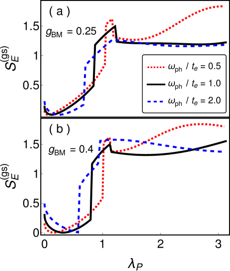
Figure 1: Ground-state e-ph entanglement entropy as a function of the effective P-coupling strength, depicted for three different values of the adiabaticity ratio and two fixed values of the BM coupling strength $g_{\textrm{BM}}$: (a) $g_{\textrm{BM}}=0.25$, and (b) $g_{\textrm{BM}}=0.4$.

Secondly, the behavior of the entanglement entropy as a function of the effective e-ph coupling strength is here markedly different from the previously investigated behavior of this quantity in the presence of Holstein-type (local) Stojanović and Vanević (2008) or P-type coupling Sto (c). Namely, in those cases the entanglement entropy grows monotonously with increasing coupling strength, regardless of whether the strong-coupling regime is characterized by the presence of sharp transitions (as in the case of P-type coupling) or just a smooth crossover (the case of Holstein-type coupling); in both cases, this entropy saturates at the value $\ln N$ (for the system size $N=8$ discussed here this maximal value is around $2.08$), which signifies maximally-entangled states Zha . Here, by contrast, the entanglement entropy shows a nonmonotonic dependence on $\lambda_{\textrm{P}}$ and does not reach the aforementioned maximal value [cf. Fig. 1].

Finally, in the special case of equal P- and BM coupling strengths the entanglement entropy vanishes, consistent with the fact that the ground state of the system in this case is a bare-excitation state (recall the discussion in Sec. II.2). It is interesting to note that in the case with $g_{\textrm{BM}}=0.4$ and the highest value $\omega_{\textrm{ph}}/t_{\rm e}=2$ of the adiabaticity ratio investigated here, the first sharp transition practically coincides with this special case of the model [for an illustration, see Fig. 1(b)].

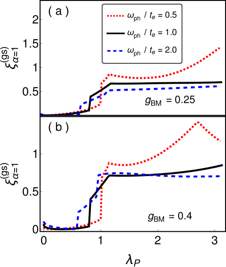
Figure 2: Dependence of the ground-state entanglement-spectrum eigenvalue $\xi^{\textrm{(gs)}}_{\alpha=1}$ on the effective P-coupling strength, shown for three different values of the adiabaticity ratio and two fixed BM coupling strengths: (a) $g_{\textrm{BM}}=0.25$, and (b) $g_{\textrm{BM}}=0.4$.

Having considered the gross features of the e-ph entanglement in the model at hand – as described by the entanglement entropy – the more subtle features can be analyzed through the prism of the corresponding entanglement spectrum. The entanglement-spectrum eigenvalues $\xi^{\textrm{(gs)}}_{\alpha}$ ($\alpha=1,2,\ldots,8$) – i.e., their dependence on $\lambda_{\textrm{P}}$ – are depicted in Figs. 2 – 5 for $\alpha=1,2,3,4$, respectively. The most apparent feature of these eigenvalues is that they reflect the presence of multiple sharp transitions in the ground state of the model under consideration. Another relevant observation is that the qualitative structure of this spectrum does not display a strong dependence on the adiabaticity ratios, i.e. it is fairly similar for different values of $\omega_{\textrm{ph}}/t_{\rm e}$. This conclusion bears some resemblance to the previously established general properties of phonon-dressed excitations formed in the presence of P-type e-ph coupling Capone et al. (1997).

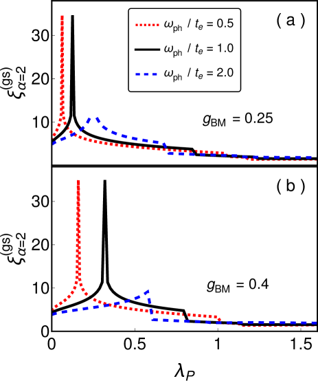
Figure 3: Dependence of the ground-state entanglement-spectrum eigenvalue $\xi^{\textrm{(gs)}}_{\alpha=2}$ on the effective P-coupling strength, shown for three different values of the adiabaticity ratio and two fixed BM coupling strengths: (a) $g_{\textrm{BM}}=0.25$, and (b) $g_{\textrm{BM}}=0.4$.

What can be inferred from Fig. 2, which shows the smallest eigenvalue $\xi^{\textrm{(gs)}}_{\alpha=1}$ in the ground-state entanglement spectrum, is that the behavior of $\xi^{\textrm{(gs)}}_{\alpha=1}$ largely mimics the beavior of the entanglement entropy itself. In other words, the dependence of $\xi^{\textrm{(gs)}}_{\alpha=1}$ on $\lambda_{\textrm{P}}$ is qualitatively similar to that of $S^{\textrm{(gs)}}_{E}$. In particular, this smallest eigenvalue also vanishes – like $S^{\textrm{(gs)}}_{E}$ itself – in the special case $g_{\textrm{P}}=g_{\textrm{BM}}$ of the model.

The last conclusion – namely, that the ground-state entanglement entropy $S^{\textrm{(gs)}}_{E}$ is to a large extent determined by the smallest entanglement-spectrum eigenvalue $\xi^{\textrm{(gs)}}_{\alpha=1}$ – is in accordance with findings of related studies of other many-body systems. To be more specific, it was already observed that the universal part of the entanglement spectrum is typically determined predominantly by the largest eigenvalues of the corresponding reduced density matrix Joh . Moreover, given that the entanglement entropy that corresponds to a certain reduced density matrix is equivalent to the thermodynamic entropy of the attendant entanglement Hamiltonian $H_{\textrm{E}}$ at the inverse temperature $\beta_{\textrm{E}}=1$ [recall the discussion in Sec. III.1], the last finding has another important implication. Namely, this finding is intimately related to the quite general issue as to whether the Hamiltonian of a generic many-body system can be thought of as being essentially encoded in a single eigenstate (e.g., its ground state). Such situations have so far been discussed only in the context of thermodynamic and entanglement entropies of single-component systems [for instance, coupled quantum spin-$1/2$ chains or interacting hard-core bosons in 1D systems Gar ]. Thus, the present study of the entanglement spectrum of a coupled e-ph model provides a qualitatively dissimilar instance of an interacting system in which the same issue is of interest.

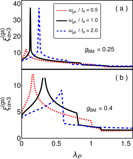
Figure 4: Dependence of the ground-state entanglement-spectrum eigenvalue $\xi^{\textrm{(gs)}}_{\alpha=3}$ on the effective P-coupling strength, shown for three different values of the adiabaticity ratio and two fixed BM coupling strengths: (a) $g_{\textrm{BM}}=0.25$, and (b) $g_{\textrm{BM}}=0.4$.

By contrast to the smallest eigenvalue, all the remaining entanglement-spectrum eigenvalues show qualitatively similar behavior as a function of $\lambda_{\textrm{P}}$. The only common feature of their dependence on $\lambda_{\textrm{P}}$ with that of $\xi^{\textrm{(gs)}}_{\alpha=1}$ is the fact that they also display the nonanalytic behavior manifesting the aforementioned sharp transitions. On the other hand, their behavior in the special case $g_{\textrm{P}}=g_{\textrm{BM}}$ of the model is drastically different than that of $\xi^{\textrm{(gs)}}_{\alpha=1}$. Namely, as can be inferred from Figs. 3 – 5 (other eigenvalues are not shown so as to avoid redundancy) all those eigenvalues display a singularity – i.e., diverge – in this special case of the model. However, given that $xe^{-x}\rightarrow 0$ as $x\rightarrow\infty$, all those eigenvalues still give vanishing contributions to the ground-state entanglement entropy in this special case of the model [cf. Eq. (25)]; in other words, $\xi^{(\textrm{gs})}_{\alpha}e^{-\xi^{(\textrm{gs})}_{\alpha}}\rightarrow 0$ for $\alpha=2,\ldots,8$ in this special case.

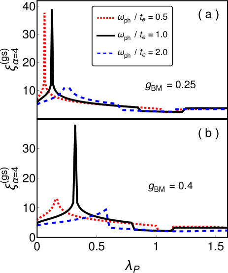
Figure 5: Dependence of the ground-state entanglement-spectrum eigenvalue $\xi^{\textrm{(gs)}}_{\alpha=4}$ on the effective P-coupling strength, shown for three different values of the adiabaticity ratio and two fixed BM coupling strengths: (a) $g_{\textrm{BM}}=0.25$, and (b) $g_{\textrm{BM}}=0.4$.

As already mentioned in Sec. II.3, in the special case $g_{\textrm{P}}=g_{\textrm{BM}}$ of the model under consideration the ground state below a critical coupling strength corresponds – after performing the Jordan-Wigner transformation – to a $W$ state. What makes the prospect of realizing $W$ states in the two proposed analog simulators of the model with simultaneous P and BM coupling  Sto (d, a) particularly appealing is the fact that this $W$ state is the actual ground state of the system in a parametrically large window of the relevant physical parameters, which is quite a rare occurrence in physical platforms for quantum computing. As a result, the envisioned realizations of $W$ states can be expected to be extremely robust.

One important aspect of the envisioned realizations of multipartite $W$ states as ground state of the model under consideration pertains to the entanglement between an itinerant excitation and bosonic degrees of freedom in the system – microwave photons in the resonators in the superconducting-qubit-based proposal of Ref. Sto (a) and quanta of vibrations in harmonic microtraps in the envisioned neutral-atom-based realizations of Ref. Sto (d). The excitation-boson entanglement in those systems – which is quantitatively described by the findings of the present study – represents a source of (boson-induced) decoherence if the condition of equality of the relevant P and BM coupling strengths is not perfectly fulfilled. The entanglement entropy can therefore be utilized as an indirect quantitative measure of bosonic contamination of sought-after $W$ states due to excitation-boson coupling. Based on the results for the entanglement entropy obtained here [cf. Fig. 1] it can be inferred that this entropy shows a relatively weak growth as a function of the residual P coupling (originating from the nonvanishing difference between $g_{\textrm{P}}$ and $g_{\textrm{BM}}$) in the immediate vicinity of the “sweet spot” $g_{\textrm{P}}=g_{\textrm{BM}}$ of the model. This bodes well for the realization of $W$ states in either of the two proposed physical platforms.

VI Summary and Conclusions

In summary, this paper investigated the ground-state entanglement spectrum and entropy of a model that describes the interplay of two of the most common mechanisms of short-ranged, nonlocal coupling of an itinerant spinless fermion excitation to zero-dimensional (dispersionless) bosons – namely, the Peierls- and breathing-mode type interactions. In order to be able to describe all the relevant physical regimes of this model, which displays sharp, level-crossing transitions at certain critical coupling strengths, the entanglement spectrum was evaluated in a numerically-exact fashion. The entanglement spectrum in the generic case of this model – with unequal strengths of the two couplings – is compared and contrasted with the special case of equal coupling strengths, in which the model supports bare-excitation Bloch eigenstates (for an arbitrary coupling strength) and even a ground state of that same type below a critical coupling strength.

It was demonstrated here that the behavior of the lowest entanglement-spectrum eigenvalue mimics that of the entanglement entropy itself; most prominently, this eigenvalue vanishes – like the entropy itself – in the special case when the Peierls and breathing-mode couplings have the same strength. Moreover, it was shown that – while reflecting the presence of sharp transitions through first-order nonanalyticities at several critical coupling strengths – all the remaining entanglement-spectrum eigenvalues also show a singularity in the case of equal coupling strengths. Finally, it was demonstrated that the entanglement entropy shows only a weak growth in the vicinity of this “sweet spot” of the model. This behavior bodes well for the realization of multipartite $W$ states in superconducting and neutral-atom based qubit arrays that may serve as analog quantum simulators of the investigated model Sto (d, a); in those systems, bare-excitation ground states of this model translate into $W$ states. Furthermore, these same systems may also serve as platforms for an experimental measurement of the entanglement spectra computed in the present work using a previously proposed general method Pichler et al. (2016) based on an analogy to the many-body Ramsey interferometry EkA .

Appendix A Derivation of the effective coupling strength

Here the expression for the effective e-ph coupling strength in the model at hand is obtained, by first finding the expressions for the P- and BM coupling strengths ($\lambda_{\textrm{P}}$ and $\lambda_{\textrm{BM}}$); the latter are derived starting from the general expression in Eq. (8).

On account of the fact that the BM coupling depends only on $q$ [cf. Eq. (7)], the Brillouin-zone average for this coupling can be expressed as

$$\langle|\gamma_{\textrm{BM}}(q)|^{2}\rangle_{\textrm{BZ}}\equiv\frac{1}{2\pi}\>\int^{\pi}_{-\pi}|\gamma_{\textrm{BM}}(q)|^{2}\>dq\>,$$ (33)

so that, as a special case of Eq. (8), one arrives at

$$\lambda_{\textrm{BM}}=\frac{(2t_{\rm e}\>\omega_{\textrm{ph}})^{-1}}{2\pi}\int^{\pi}_{-\pi}\>|\gamma_{\textrm{BM}}(q)|^{2}\>dq\>.$$ (34)

By making use of Eq. (7), from the last equation one straightforwardly obtains

$$\lambda_{\textrm{BM}}=\frac{(2t_{\rm e}\>\omega_{\textrm{ph}})^{-1}}{2\pi}\times 4g^{2}_{\textrm{BM}}\>\omega^{2}_{\textrm{ph}}\int^{\pi}_{-\pi}\sin^{2}q\>dq\>,$$ (35)

which finally leads to

$$\lambda_{\textrm{BM}}=g^{2}_{\textrm{BM}}\>\frac{\omega_{\textrm{ph}}}{t_{\rm e}}\>.$$ (36)

At the same time, given that the P-coupling vertex function depends both on $k$ and $q$ [cf. Eq. (6)], the corresponding Brillouin-zone average ought to involve integrations over both excitation- and phonon quasimomenta, i.e.,

$$\langle|\gamma_{\textrm{P}}(k,q)|^{2}\rangle_{\textrm{BZ}}\equiv\frac{1}{(2\pi)^{2}}\>\int^{\pi}_{-\pi}\int^{\pi}_{-\pi}\>|\gamma_{\textrm{P}}(k,q)|^{2}\>dkdq\>.$$ (37)

Therefore, $\lambda_{\textrm{P}}$ is given by [cf. Eq. (8)]

$$\lambda_{\textrm{P}}=\frac{(2t_{\rm e}\>\omega_{\textrm{ph}})^{-1}}{(2\pi)^{2}}\int^{\pi}_{-\pi}\int^{\pi}_{-\pi}\>|\gamma_{\textrm{P}}(k,q)|^{2}\>dkdq\>,$$ (38)

which, using Eq. (6), further reduces to

$$\lambda_{\textrm{P}} = \frac{(2t_{\rm e}\>\omega_{\textrm{ph}})^{-1}}{(2\pi)^{2}}\>\times 4g^{2}_{\textrm{P}}\>\omega^{2}_{\textrm{ph}}$$ (39)

$$\times \int^{\pi}_{-\pi}\int^{\pi}_{-\pi}[\sin(k+q)-\sin k]^{2}\>dkdq\>.$$

By evaluating the integral in the last equation,

$$\int^{\pi}_{-\pi}\int^{\pi}_{-\pi}[\sin(k+q)-\sin k]^{2}\>dkdq=4\pi^{2}\>,$$ (40)

and inserting this last result into Eq. (39), one finally obtains

$$\lambda_{\textrm{P}}=2g^{2}_{\textrm{P}}\>\frac{\omega_{\textrm{ph}}}{t_{\rm e}}\>.$$ (41)

It is worthwhile noting that the total effective e-ph coupling strength $\lambda_{\textrm{e-ph}}$ [cf. Eq. (8)] is here given by the simple sum of $\lambda_{\textrm{P}}$ and $\lambda_{\textrm{BM}}$, i.e.

$$\lambda_{\textrm{e-ph}}=\lambda_{\textrm{P}}+\lambda_{\textrm{BM}}=(2g^{2}_{\textrm{P}}+g^{2}_{\textrm{BM}})\>\frac{\omega_{\textrm{ph}}}{t_{\rm e}}\>.$$ (42)

Namely, while the expression for $\langle|\gamma_{\textrm{e-ph}}(k,q)|^{2}\rangle_{\textrm{BZ}}$ [cf. Eq. (8)] in the case of simultaneous P and BM couplings also contains the cross terms originating from the product of the P and BM vertex functions [cf. Eqs. (6) and (7)], it is straightforward to show that their BZ average – which entails integrals over $k,q\in(-\pi,\pi]$ – is equal to zero; thus, those terms do not contribute to $\lambda_{\textrm{e-ph}}$.

Appendix B Derivation of the reduced density matrix $\rho^{(\textrm{gs})}_{\textrm{e}}$

In what follows, an explicit derivation is provided of the expression for the matrix elements of the reduced density matrix $\rho^{(\textrm{gs})}_{\textrm{e}}$ [cf. Eq. (52)] corresponding to the ground state $|\psi_{\textrm{gs}}\rangle$ of the system.

The ground state $|\psi_{\textrm{gs}}\rangle$ belongs to the $K=K_{\textrm{gs}}$ sector of the Hilbert space of the system [recall the discussion in Sec. IV]. Therefore, this state can be expanded as [cf. Eq. (31)]

$$|\psi_{\textrm{gs}}\rangle=\sum_{\mathbf{m}}C_{K_{\textrm{gs}},\mathbf{m}}|K_{\textrm{gs}},\mathbf{m}\rangle\>,$$ (43)

where $|K_{\textrm{gs}},\mathbf{m}\rangle$ is the symmetry-adapted basis of that Hilbert-space sector [cf. Eq. (28)]:

$$|K_{\textrm{gs}},\mathbf{m}\rangle=N^{-1/2}\sum_{n=1}^{N}e^{iK_{\textrm{gs}}n}\,|n\rangle_{\text{e}}\otimes\mathcal{T}^{\textrm{ph}}_{n-1}|\mathbf{m}\rangle_{\text{ph}}\>.$$ (44)

By making use of the expansion in Eq. (43), the corresponding density matrix of the e-ph system can be written in the form

$$\rho^{\textrm{(gs)}}_{\textrm{e-ph}}=\sum_{\mathbf{m},\mathbf{m^{\prime}}}\>C^{*}_{K_{\textrm{gs}},\mathbf{m^{\prime}}}\>C_{K_{\textrm{gs}},\mathbf{m}}\>|K_{\textrm{gs}},\mathbf{m}\rangle\langle K_{\textrm{gs}},\mathbf{m^{\prime}}|\>.$$ (45)

Using Eq. (44), it further follows that

$$\rho^{\textrm{(gs)}}_{\textrm{e-ph}} = N^{-1}\sum_{\mathbf{m},\mathbf{m^{\prime}}}\sum^{N}_{n,n^{\prime}=1}\>e^{iK_{\textrm{gs}}(n-n^{\prime})}C^{*}_{K_{\textrm{gs}},\mathbf{m^{\prime}}}\>C_{K_{\textrm{gs}},\mathbf{m}}\>$$ (46)

$$\times |n\rangle\langle n^{\prime}|\otimes|\mathcal{T}^{\textrm{ph}}_{n-1}\mathbf{m}\rangle\langle\mathcal{T}^{\textrm{ph}}_{n^{\prime}-1}\mathbf{m^{\prime}}|\>.$$

According to Eq. (23), the reduced excitation density matrix $\rho^{(\textrm{gs})}_{\textrm{e}}$ can now be obtained by tracing the density matrix $\rho^{\textrm{(gs)}}_{\textrm{e-ph}}$ over the phonon basis. In other words,

$$\rho^{(\textrm{gs})}_{\textrm{e}}=\sum_{\mathbf{m^{\prime\prime}}}\langle\mathbf{m^{\prime\prime}}|\>\rho^{\textrm{(gs)}}_{\textrm{e-ph}}\>|\mathbf{m^{\prime\prime}}\rangle\>,$$ (47)

where $\mathbf{m^{\prime\prime}}$ is the dummy index for the phonon basis states [i.e., $\{\mathbf{m^{\prime\prime}}\}$ represents the set of all phonon occupation-number configurations]. By inserting $\rho^{\textrm{(gs)}}_{\textrm{e-ph}}$ from Eq. (46), one obtains

$$\rho^{(\textrm{gs})}_{\textrm{e}} = N^{-1}\sum_{\mathbf{m},\mathbf{m^{\prime}},\mathbf{m^{\prime\prime}}}\sum^{N}_{n,n^{\prime}=1}\>e^{iK_{\textrm{gs}}(n-n^{\prime})}C^{*}_{K_{\textrm{gs}},\mathbf{m^{\prime}}}\>C_{K_{\textrm{gs}},\mathbf{m}}\>$$ (48)

$$\times \>\langle\mathcal{T}^{\textrm{ph}}_{n^{\prime}-1}\mathbf{m^{\prime}}|\mathbf{m^{\prime\prime}}\rangle\langle\mathbf{m^{\prime\prime}}|\mathcal{T}^{\textrm{ph}}_{n-1}\mathbf{m}\rangle\>|n\rangle\langle n^{\prime}|\>.$$

At this point it is convenient to first carry out the summation over $\mathbf{m^{\prime\prime}}$. By making use of the completeness relation in the phonon Hilbert space

$$\sum_{\mathbf{m^{\prime\prime}}}|\mathbf{m^{\prime\prime}}\rangle\langle\mathbf{m^{\prime\prime}}|=\mathbbm{1}_{D_{\textrm{ph}}}\>,$$ (49)

where $\mathbbm{1}_{D_{\textrm{ph}}}$ is the identity operator in that space, it is straightforward to verify that

$$\sum_{\mathbf{m^{\prime\prime}}}\langle\mathcal{T}^{\textrm{ph}}_{n^{\prime}}\mathbf{m^{\prime}}|\mathbf{m^{\prime\prime}}\rangle\langle\mathbf{m^{\prime\prime}}|\mathcal{T}^{\textrm{ph}}_{n}\mathbf{m}\rangle=\langle\mathcal{T}^{\textrm{ph}}_{n^{\prime}-1}\mathbf{m^{\prime}}|\mathcal{T}^{\textrm{ph}}_{n-1}\mathbf{m}\rangle\>.$$ (50)

Using this last result, the expression for $\rho^{(\textrm{gs})}_{\textrm{e}}$ in Eq. (48) now reduces to

$$\rho^{(\textrm{gs})}_{\textrm{e}} = N^{-1}\sum_{\mathbf{m},\mathbf{m^{\prime}}}\sum^{N}_{n,n^{\prime}=1}\>e^{iK_{\textrm{gs}}(n-n^{\prime})}C^{*}_{K_{\textrm{gs}},\mathbf{m^{\prime}}}\>C_{K_{\textrm{gs}},\mathbf{m}}\>$$ (51)

$$\times \>\langle\mathcal{T}^{\textrm{ph}}_{n^{\prime}-1}\mathbf{m^{\prime}}|\mathcal{T}^{\textrm{ph}}_{n-1}\mathbf{m}\rangle\>|n\rangle\langle n^{\prime}|\>.$$

The last expression implies that the matrix elements of the reduced excitation density matrix are given by

$$\left(\rho^{(\textrm{gs})}_{\textrm{e}}\right)_{nn^{\prime}} = N^{-1}\>e^{iK_{\textrm{gs}}(n-n^{\prime})}\sum_{\mathbf{m},\mathbf{m^{\prime}}}\>C^{*}_{K_{\textrm{gs}},\mathbf{m^{\prime}}}\>C_{K_{\textrm{gs}},\mathbf{m}}$$ (52)

$$\times \>\langle\mathbf{m^{\prime}}\>|\>\mathcal{T}^{\textrm{ph}}_{n-n^{\prime}}\mathbf{m}\rangle\>,$$

where use has been made of the fact that $\langle\mathcal{T}^{\textrm{ph}}_{n^{\prime}}\mathbf{m^{\prime}}\>|\>\mathcal{T}^{\textrm{ph}}_{n}\mathbf{m}\rangle\equiv\langle\mathbf{m^{\prime}}\>|\>\mathcal{T}^{\textrm{ph}}_{n-n^{\prime}}\mathbf{m}\rangle$.

References

- (1) For a review, see N. Laflorencie, Phys. Rep. 646, 1 (2016).
- Li and Haldane (2008) H. Li and F. D. M. Haldane, Phys. Rev. Lett. 101, 010504 (2008).
- Fidkowski (2010) L. Fidkowski, Phys. Rev. Lett. 104, 130502 (2010).
- Pollmann et al. (2010) F. Pollmann, E. Berg, A. M. Turner, and M. Oshikawa, Phys. Rev. B 81, 064439 (2010).
- Thomale et al. (2010) R. Thomale, A. Sterdyniak, N. Regnault, and B. A. Bernevig, Phys. Rev. Lett. 104, 180502 (2010).
- Poilblanc (2010) D. Poilblanc, Phys. Rev. Lett. 105, 077202 (2010).
- Läuchli and Schliemann (2012) A. M. Läuchli and J. Schliemann, Phys. Rev. B 85, 054403 (2012).
- (8) S. Wu, X. Ran, B. Yin, Q.-F. Li, B.-B. Mao, Y.-C. Wang, and Z. Yan, Phys. Rev. B , 155121 (2023).
- (9) Z. Yan and Z. Y. Meng, Nat. Commun. , 2360 (2023).
- Schliemann (2011) J. Schliemann, Phys. Rev. B 83, 115322 (2011).
- (11) X. Deng and L. Santos, Phys. Rev. B , 085138 (2011).
- Ejima et al. (2014) S. Ejima, F. Lange, and H. Fehske, Phys. Rev. Lett. 113, 020401 (2014).
- Parisen Toldin and Assaad (2018) F. Parisen Toldin and F. F. Assaad, Phys. Rev. Lett. 121, 200602 (2018).
- Yang et al. (2015) Z.-C. Yang, C. Chamon, A. Hamma, and E. R. Mucciolo, Phys. Rev. Lett. 115, 267206 (2015).
- Geraedts et al. (2017) S. D. Geraedts, N. Regnault, and R. M. Nandkishore, New J. Phys. 19, 113021 (2017).
- (16) R. Jafari and A. Akbari, Phys. Rev. A 103, 012204 (2021).
- (17) L. Zhou, Phys. Rev. Res. 4, 043164 (2022).
- (18) L.-N. Luan, M.-Y. Zhang, and L.-C. Wang, Physica A 604, 127866 (2022); Chinese Phys. B 32, 090302 (2023).
- (19) For an extensive review, see L. Amico, R. Fazio, A. Osterloh, and V. Vedral, Rev. Mod. Phys. , 517 (2008).
- (20) See, e.g., A. Wehrl, Rev. Mod. Phys. , 221 (1978).
- Hayashi (2017) M. Hayashi, A Group Theoretic Approach to Quantum Information (Springer, Berlin, 2017).
- Chandran et al. (2014) A. Chandran, V. Khemani, and S. Sondhi, Phys. Rev. Lett. 113, 060501 (2014).
- Sto (c) V. M. Stojanović, Phys. Rev. B , 134301 (2020).
- (24) G. Roósz and K. Held, Phys. Rev. B , 195404 (2022).
- (25) K. Hannewald, V. M. Stojanović, and P. A. Bobbert, J. Phys.: Condens. Matter , ().
- Hannewald et al. (2004) K. Hannewald, V. M. Stojanović, J. M. T. Schellekens, P. A. Bobbert, G. Kresse, and J. Hafner, Phys. Rev. B 69, 075211 (2004).
- Rösch et al. (2005) O. Rösch, O. Gunnarsson, X. J. Zhou, T. Yoshida, T. Sasagawa, A. Fujimori, Z. Hussain, Z.-X. Shen, and S. Uchida, Phys. Rev. Lett. 95, 227002 (2005).
- (28) C. Slezak, A. Macridin, G. A. Sawatzky, M. Jarrell, and T. A. Maier, Phys. Rev. B , ().
- (29) N. Vukmirović, V. M. Stojanović, and M. Vanević, Phys. Rev. B , 041408(R) (2010).
- (30) V. M. Stojanović, N. Vukmirović, and C. Bruder, Phys. Rev. B , 165410 (2010).
- Vuk (b) N. Vukmirović, C. Bruder, and V. M. Stojanović, Phys. Rev. Lett. , 126407 (2012).
- Shn (a) E. I. Shneyder, S. V. Nikolaev, M. V. Zotova, R. A. Kaldin, and S. G. Ovchinnikov, Phys. Rev. B , 235114 (2020).
- Shn (b) E. I. Shneyder, M. V. Zotova, S. V. Nikolaev, and S. G. Ovchinnikov, Phys. Rev. B , 155153 (2021).
- (34) For a review, see J. Ranninger, in Proc. Int. School of Physics “E. Fermi”, Course CLXI, edited by G. Iadonisi, J. Ranninger, and G. De Filippis (IOS Press, Amsterdam, 2006), pp. 1–25.
- Alexandrov and Devreese (2010) A. S. Alexandrov and J. T. Devreese, Advances in Polaron Physics (Springer-Verlag, Berlin, 2010).
- Ranninger and Thibblin (1992) J. Ranninger and U. Thibblin, Phys. Rev. B 45, 7730 (1992).
- Capone et al. (1997) M. Capone, W. Stephan, and M. Grilli, Phys. Rev. B 56, 4484 (1997).
- (38) G. Wellein and H. Fehske, Phys. Rev. B , 4513 (1997); ibid. , 6208 (1998).
- Jeckelmann and White (1998) E. Jeckelmann and S. R. White, Phys. Rev. B 57, 6376 (1998).
- Bonča et al. (1999) J. Bonča, S. A. Trugman, and I. Batistić, Phys. Rev. B 60, 1633 (1999).
- Zoli (2003) M. Zoli, Phys. Rev. B 67, 195102 (2003).
- Stojanović et al. (2004) V. M. Stojanović, P. A. Bobbert, and M. A. J. Michels, Phys. Rev. B 69, 144302 (2004).
- Stojanović et al. (2012) V. M. Stojanović, T. Shi, C. Bruder, and J. I. Cirac, Phys. Rev. Lett. 109, 250501 (2012).
- Mei et al. (2013) F. Mei, V. M. Stojanović, I. Siddiqi, and L. Tian, Phys. Rev. B 88, 224502 (2013).
- Chakraborty et al. (2016) M. Chakraborty, N. Mohanta, A. Taraphder, B. I. Min, and H. Fehske, Phys. Rev. B 93, 155130 (2016).
- (46) D. Jansen, J. Stolpp, L. Vidmar, and F. Heidrich-Meisner, Phys. Rev. B , 155130 (2019).
- Holstein (1959) T. Holstein, Ann. Phys. (N.Y.) 8, 343 (1959).
- Stojanović and Vanević (2008) V. M. Stojanović and M. Vanević, Phys. Rev. B 78, 214301 (2008).
- Ger (a) B. Gerlach and H. Löwen, Phys. Rev. B , (); , ().
- Ger (b) B. Gerlach and H. Löwen, Rev. Mod. Phys. , 63 (1991).
- (51) H. Fröhlich, Adv. Phys. , 325 (1954).
- (52) J. Sous, M. Chakraborty, C. P. J. Adolphs, R. V. Krems, and M. Berciu, Sci. Rep. , 1169 (2017).
- Stojanović et al. (2014) V. M. Stojanović, M. Vanević, E. Demler, and L. Tian, Phys. Rev. B 89, 144508 (2014).
- Stojanović and Salom (2019) V. M. Stojanović and I. Salom, Phys. Rev. B 99, 134308 (2019).
- (55) J. K. Nauth and V. M. Stojanović, Phys. Rev. B , 174306 (2023).
- Sto (d) V. M. Stojanović, Phys. Rev. A , 022410 (2021).
- (57) See, e.g., P. Coleman, Introduction to Many-Body Physics (Cambridge University Press, Cambridge, UK, 2015).
- Sto (a) V. M. Stojanović, Phys. Rev. Lett. , 190504 (2020).
- Zha (c) G. Q. Zhang, W. Feng, W. Xiong, D. Xu, Q. P. Su, and C. P. Yang, Phys. Rev. Appl. 20, 044014 (2023).
- Sto (c) V. M. Stojanović and J. K. Nauth, Phys. Rev. A 106, 052613 (2022).
- (61) V. M. Stojanović and J. K. Nauth, Phys. Rev. A 108, 012608 (2023).
- Engelsberg and Schrieffer (1963) S. Engelsberg and J. R. Schrieffer, Phys. Rev. 131, 993 (1963).
- (63) T. Haase, G. Alber, and V. M. Stojanović, Phys. Rev. Res. 4, 033087 (2022).
- Cullum and Willoughby (1985) J. K. Cullum and R. A. Willoughby, Lanczos Algorithms for Large Symmetric Eigenvalue Computations (Birkhäuser, Boston, 1985).
- (65) P. Prelovšek and J. Bonča, in Strongly Correlated Systems: Numerical Methods, edited by A. Avella and F. Mancini (Springer, Berlin, 2013), chap. 1, pp. 1-29.
- (66) E. Schmidt, Math. Ann. , 433 (1907).
- (67) For an introduction, see, e.g., A. Ekert and P. L. Knight, Am. J. Phys. , 415 (1995).
- (68) W. H. Press, S. A. Teukolsky, W. T. Vetterling, and B. P. Flannery, Numerical Recipes in C: The Art of Scientific Computing (Cambridge University Press, Cambridge, 1999).
- (69) Y. Zhao, P. Zanardi, and G. Chen, Phys. Rev. B , 195113 (2004).
- (70) S. Johri, D. S. Steiger, and M. Troyer, Phys. Rev. B , 195136 (2017).
- (71) J. R. Garrison and T. Grover, Phys. Rev. X , 021026 (2018).
- Pichler et al. (2016) H. Pichler, G. Zhu, A. Seif, P. Zoller, and M. Hafezi, Phys. Rev. X 6, 041033 (2016).
- (73) A. K. Ekert, C. M. Alves, D. K. L. Oi, M. Horodecki, P. Horodecki, and L. C. Kwek, Phys. Rev. Lett. , 217901 (2002).