ANDRÉS ARCONES et al. \titlemarkMODEL BIAS IDENTIFICATION FOR BAYESIAN CALIBRATION OF STOCHASTIC DIGITAL TWINS OF BRIDGES
Daniel Andrés Arcones, Department 7.7 Modeling and Simulation, Bundesanstalt für Materialforschung und -prüfung, Unter den Eichen 87, 12205 Berlin, Germany.
Priority Program (SPP) 2388/1 "Hundred plus" of the German Research Foundation (Deutsche Forschungsgemeinschaft, DFG) - Project number 501811638.
Model bias identification for Bayesian calibration of stochastic digital twins of bridges
Abstract
[Abstract]Simulation-based digital twins must provide accurate, robust and reliable digital representations of their physical counterparts. Quantifying the uncertainty in their predictions plays, therefore, a key role in making better-informed decisions that impact the actual system. The update of the simulation model based on data must be then carefully implemented. When applied to complex standing structures such as bridges, discrepancies between the computational model and the real system appear as model bias, which hinders the trustworthiness of the digital twin and increases its uncertainty. Classical Bayesian updating approaches aiming to infer the model parameters often fail at compensating for such model bias, leading to overconfident and unreliable predictions. In this paper, two alternative model bias identification approaches are evaluated in the context of their applicability to digital twins of bridges. A modularized version of Kennedy and O’Hagan’s approach and another one based on Orthogonal Gaussian Processes are compared with the classical Bayesian inference framework in a set of representative benchmarks. Additionally, two novel extensions are proposed for such models: the inclusion of noise-aware kernels and the introduction of additional variables not present in the computational model through the bias term. The integration of such approaches in the digital twin corrects the predictions, quantifies their uncertainty, estimates noise from unknown physical sources of error and provides further insight into the system by including additional pre-existing information without modifying the computational model.
\jnlcitation\cname, , , and . \ctitleModel bias identification for Bayesian calibration of stochastic digital twins of bridges. \cjournalASMBI \cvol2021;00(00):1–18.
keywords:
Model bias, Bayesian updating, digital twins, uncertainty quantification1 Introduction
The extended availability of computational means in recent years has prompted the digitalization of a plethora of processes across industries. Nowadays, it is not unusual for practitioners, managers and engineers to have large quantities of data at their disposal to enhance their predictions and guide their decisions. Digital twins are key for efficiently harnessing such an amount of information. This is not different in the field of structural engineering and bridge management, where the utilization of digital twins of bridges provides immediate access to the past, current and future state of the structure. Nevertheless, one of the main challenges for its widespread implementation is the lack of homogenization and standardization in their definition and implementation1. Assuring the fidelity, accuracy and reliability of any particular digital twin and its predictions is therefore crucial in the absence of a common framework within which to evaluate its quality. This holds especially true for their applications to structures such as bridges, whose safety and integrity must be preserved under any condition. The objective of this work is to reliably quantify the discrepancy between model and observations in the context of stochastic simulation-based digital twins of bridges to assure their safe and robust deployment for real applications.
Despite considerable efforts, a concrete universally accepted definition of what is a digital twin is yet to be found2. Probably the most extended definition of a digital twin is the one given by Grieves and Vickers, who consider it as “a set of virtual information constructs that fully describe a potential or actual physical manufactured product from the micro atomic level to the macro geometrical level"3. However, this definition is too general for the context of this paper, which will focus on the representation and response of digital twins of bridges. We will alternatively consider the definition from Lu et al., where they refer to "a digital replica of physical assets, processes, and systems. Digital twins integrate artificial intelligence, machine learning, and data analytics to create living digital simulation models that can learn and update from multiple sources as well as represent and predict the current and future conditions of physical counterparts."4
In contrast to geometry-based digital twins, with a focus on geometrical representation of the information such as Building Information Models (BIM), and purely data-driven digital twins, which focus on sensor observations and monitoring, simulation-based digital twins complement the established knowledge from the system, present in a simulation model, with sensor observations. This allows for the calibration of a representation of the real state of the system that can be used to generate predictions on Quantities of Interest (QoI), while also posing further challenges. In particular, these predictions often present discrepancies when compared with sensor observations, which reduces their reliability5. To generate useful models that reflect their real counterparts, it is not only imperative to appropriately tune their associated parameters but also to improve the model where necessary. The update of the simulation model is often an iterative process guided by the available data and the requirements imposed on the model. As new data becomes available, the model may need to be updated or modified. Leveraging the available data and accounting for the shortcomings of the model pose a real challenges for keeping the simulation models of digital twins true to the observations and the real state of the system.
One of the most popular methods to tune simulation models is using Bayesian inference approaches to estimate the latent parameters. This approach introduces information obtained from observations to update the models built following known physical laws. Due to its probabilistic nature, uncertainty quantification is also naturally included in the evaluation. The introduction of this uncertainty quantification implies a stochastic component in the predictions and definition of the digital twin. Additionally, as new measurements are obtained, the estimated model can be easily updated to reflect the new reality of the real system. This adaptability is obtained at the expense of often requiring reliable prior information on the potential values of the model parameters and needing numerous evaluations of usually very costly models. In structural and civil engineering, model updating using Bayesian inference has been applied to numerous aspects of the design and monitoring of structures. Material laws and constitutive relations are modified to reflect the behaviour of the real system6, 7, 8, 9, 10. The models that represent the structure are updated to match the observations11, 12, 13. In cases where the structural model presents a heterogeneous material behaviour, Bayesian inference methods are used to obtain the parameters of the representation of the material variability 14. For the case of bridges, SHM systems are calibrated following this methodology 15, bridge model parameters are obtained using data from measurement campaigns 16 and digital twins are tuned to represent the response of a bridge in real time17.
Three main challenges arise when implementing a Bayesian framework for digital twins of structures such as bridges: data availability, model complexity and compatibility in the implementation18. Typically, large quantities of data are required for an accurate model updating, but sensor systems, despite providing continuous data streams over time, are usually limited to sparsely distributed observation points. Therefore, the fidelity of the prediction depends to a large extent on the data richness and quality. On the other hand, complex models are often unavoidable in the case of simulation-based digital twins. Surrogate models are then introduced as substitutes in time-sensitive applications or to reduce the computational cost for the Bayesian inference at the expense of introducing further uncertainties5, 19, 20. Finally, a large selection of software tools has been developed in recent years that allow for simplified implementations of Bayesian frameworks in larger digital set-ups. Examples of them are emcee21, PyMC22, stan23, UQpy24 or probeye25. In this project, the model updating schemes are implemented using probeye, which is an open-source package for Python developed to this end. However, no matter how finely tuned or complex a model is, it will still be limited by its own definition based on a set of prescribed assumptions. The reality, in contrast, is infinitely complex and will never be fully described by a computational model26. In the particular case of models updated in a Bayesian framework, the dependency on the training dataset often leads to overfitted and overconfident models that do not reflect the real system 27. One of the main targets of this work is precisely the quantification of those model discrepancies rooted in deficiencies in the model definition.
For a proper evaluation of the fidelity and reliability of a model, we find it essential to quantify explicitly the discrepancy between the model and the real system. For the purpose of this paper, we will define as model inadequacies all deviations in the behaviour of any subcomponent of the computational model when compared with a hypothetical real system. This applies to deviations in the value of the model parameters, boundary and initial conditions, variations in the constitutive law or directly the presence of effects in the real system that are not captured by the model. We will define as model bias or model discrepancy indistinctively the additive correction term necessary to compensate for the difference in outputs of the computational model and real system. This is coherent with the definition of model bias as typically implemented following Kennedy and O’Hagan’s framework28. In this paper, we will address the quantification of such a model bias paying special attention to its interpretation, leaving the model inadequacies at subcomponent level out of scope.
The inclusion of model bias in the inverse problem formulation not only allows quantifying the discrepancy between model and observations, but is also able to improve the inference procedure29. However, the introduction of an overly flexible term to fully capture the model bias incurs potential identifiability issues 30. Throughout the years, several approaches have tried to tackle the identifiability issue, some of which are promising alternatives for their implementation in a digital twin. Brynjardóttir and O’Hagan31 highlight the impact of the choice of priors for the bias distribution, outlining the importance of elicitation and expert knowledge in their definition. Modularized versions of Kennedy and O’Hagan’s framework32 attempt to separate the effects of calibrating the model parameter from the bias. Successful examples are its application to energy systems33 and building energy transference estimation34. Alternatively, embedded approaches associate additively the bias term with the corresponding latent parameter35 or subcomponents of the system36, and have successfully been applied to composite rotor blades37, rocket ignition mechanisms35, jet turbulences 38 and healthcare policy models36, 39. Finally, modelling the bias term as Orthogonal Gaussian Processes (OGPs) 40 has been proposed as an alternative solution to prevent the identifiability problem between latent and bias parameters while recovering control over the optimality of the process. In this paper, we will compare the suitability of a modularized implementation of the model bias identification framework and the inclusion of OGPs. These two methods are the least intrusive for identifying the model bias, especially in comparison to embedded approaches, this makes them very attractive for digital twins, where modifications of the model are not always possible. To our knowledge, none of these approaches has been implemented or evaluated in the context of digital twins of bridges. Correlated or non-additive bias structures are out of the scope of this paper due to the increased complexity and amount of system information required for their implementation, which may not necessarily be available.
As previously mentioned, the aim of this study is to implement, assess and extend a model bias identification methodology to be applied to digital twins of bridges, mitigating some of the problems present in Bayesian updating. In particular, we will show that including a bias term corrects the predictions, enhances the model and provides more reliable uncertainty thresholds. Three different approaches will be evaluated: the classical Bayesian inference approach without bias, a modularized version of Kennedy and O’Hagan’s framework32, and a modification of the same framework to include OGPs in the model bias definition40. To further take advantage of the particularities of Digital Twins, two novel extensions based on the bias formulation are developed in this work: the quantification of noise from physical sources in the systems response and the extension of the input domain with additional variables. On the one hand, the sensor’s network of the Digital Twin often provides a continuous stream of data that is susceptible to present variations due to unaccounted sources. Due to the existence of discrepancies between model and reality, the variance produced by such sources cannot be quantified adequately in many cases, as the model bias is often included in the noise estimation, leading to inaccurate results. The introduction of noise-aware kernels in the bias term enables such a quantification. On the other hand, Digital Twins present at their disposal a plethora of information sources that can be used to enrich the model. However, adapting the computational model to include them typically implies increasing its complexity and it is often not possible. Our proposed extension of the model bias term includes the desired additional variables non-intrusively, providing insight into their influence on the model. Both extensions will be implemented for the aforementioned approaches of interest in the context of Digital Twins of bridges.
The different approaches will be presented in Section 2 and applied in Section 3. First, in Section 3.1, we will use a simple 1D example to compare how accurate the inferred parameters with each of the approaches are and evaluate their capacity to quantify the model bias. Then, in Section 3.2, we will analyze in a stochastic cantilever beam system based on a cantilever bridge their ability to quantify the noise from non-prescribed sources and the possibility to include heteroscedastic noise structures with physical meaning. Finally, in Section 3.3, we will implement each of the approaches to a simplified illustrative model based on a real bridge. We will prove how it is possible to include additional information external to the model, such as a temperature variation, to compensate for the bias in the model related to it. The comparisons will always be done under the optic of their potential application to a digital twin. Section 4 closes with the conclusions and potential extensions.
2 Methodology
The computational model is defined as a -real valued function over a -dimensional domain such that . Ultimately, the goal is to obtain a computational model that behaves as the real system , represented as an analogously defined function. The computational model takes as input a set of system coordinates , is defined by a set of latent parameters and a set of prescribed parameters and produces an output . In this paper, denotes the input variable of , denotes a discrete realization of represented as a -dimensional vector, denotes a sample of discrete realizations represented as a matrix, and denotes the -th entry of . In practice, corresponds to the input coordinates at which one observation takes place, e.g. a sensor’s spatial coordinates, and the set of input coordinates where each of the observations takes place. Following the same notation, represents the set of observations employed to fit the parameters of . These observations are assumed to be produced by a generative process defined as a -real valued function. The observations may not only depend on but also admit the coordinates as an extended input not included in , with its associated set of realizations . An example of such variable may be a set of time or temperature coordinates that are known for each observation but not considered by the computational model . Then, the generative process is defined as . These observations are generally provided by physical sensors with a prescribed measurement noise , which corresponds to the difference between observations and real system . Analogously, the real system is defined as a function . In a general continuous way, we can formulate the problem as
| (1) |
where is an additional error term indicating the discrepancy between the computational model and reality, necessary to achieve the equality. For example, such a formulation can be applied to the calibration of the Young’s modulus of a linear elastic cantilever beam under self-weight. We consider as the set of spatial coordinates that identify the different points of the beam. The cantilever beam deformation is governed by its Young’s modulus , which would be the latent parameter and other material and geometry parameters such as length, density, Poisson’s ratio, etc., that are encoded in . The set of equations of linear elasticity that for a given provides the deformation of this specific beam at a position is the computational model . The real deformations of the cantilever beam are defined by , which follows an infinitely complex law. Moreover, does not only depend on , but on other parameters , such as the temperature of the beam. The discrepancy between and due to the necessary simplifications in the system are , which can explicitly include the temperature dependency , present in but not in . Finally, would be observed through some type of sensor, image correlation for example, that introduces a noise in the measurement , which may be different for every point and at every temperature.
During this paper, the parameters will not be explicitly included in the formulation to avoid excessive notation. If we consider only a discrete set of observations, then the relationship is transformed to Equation 2:
| (2) |
An important modelling choice resides in the structure of the error terms and . The term defines exclusively the prescribed noise from the sensor. It is generally provided by the manufacturer in the cases of physical sensors or prescribed in the case of virtual ones. Noise will be added to the covariance matrix of the predictions from . For simplicity, it will be considered uncorrelated Gaussian noise with a prescribed amplitude . The term corresponds to the manifestation of the model discrepancy to the observed quantities, which is the object of this study. The reduction of is a model identification problem, usually following an iterative approach. In this context, changes to the model are introduced to better match the available information and minimize the discrepancy with the real system. This model update must then consider the available data to identify the fitting parameters and guide potential further improvements in subsequent iterations.
The objective of the parameter identification approaches for one of such iterations is to find parameters from Equation 2 such that the deviation of the computational from the physical system is minimized. This deviation can be quantified in many different ways depending on what is understood as the “best-fitting" parameters . A classical metric for such an approach is the Mean Squared Error (MSE), under which the problem reduces to solving:
| (3) |
This concept can be extended to a functional analysis framework, allowing to define losses over the functions and instead of its observations. The main loss considered in this paper is the loss, although other options such as can be implemented as well. The loss is generated from the homonymous norm in its associated Hilbert space, being analogous to the MSE in a functional sense40:
| (4) |
where is the domain of evaluation of the norm and no additional variables are considered. The evaluation of such a loss in its continuous form is not possible in practice, hence discretization is required. The main difference with MSE is that depends on the discretization of the loss itself while MSE relies exclusively on the observations, which provides more flexibility. This is particularly useful for the case that sparse observations do not correspond with the points of interest, which can make use of alternative discretizations to cover them.
The inverse problem minimizes any of the previous losses varying . A priori, these metrics would require extensive knowledge about both the generative and the computational model, but they would achieve the best possible fit under a given set of conditions. If the samples represent sufficiently well the domain of the generative process and the predictions are generated with enough information from the computational model, MSE and losses tend to the same value.
2.1 Bayesian inference without bias
Bayesian inference approaches are based on the well-known Bayes theorem
| (5) |
where is the posterior distribution that describes the probability of the parameter of having generated , represent the prior distribution based on the beliefs about before seeing the data, is the likelihood function that represents the probability of observing for a given and is the marginal probability of observing . The prior must be prescribed, and the likelihood term will consider a Gaussian error model on the residuals with noise . Iterative approaches such as Monte Carlo-Markov Chains (MCMC) converge to an estimation of the posterior distribution up to a constant such that , avoiding the calculation of 41. In this work, an MCMC algorithm with Metropolis-Hastings selection criteria19 will be applied to the parameter identification problem. This classical approach is well established and admits multiple modifications to improve its efficiency.
However, the application of classical Bayesian inference approaches presents three relevant shortcomings. First, the results obtained depend completely on the prescribed forward model and its assumptions. Modelling complex real systems requires simplifications from the geometry, governing laws or relevant parameters that cannot be quantified by an unbiased approach. The inferred parameters are intrinsic to the real system and have a meaning on their own. Due to the aforementioned simplifications, those parameters estimated through unbiased approaches will converge to values that may differ from those that would best describe the real system as a whole and present high confidence in the result. This is even more relevant in those cases where the model bias is pronounced the most. In digital twins of structures such as bridges, the simulation models tend to be extremely complex and sensors are sparse in space, which simultaneously increases the potential discrepancy between model predictions and observations due to the complexity, and the risk of overfitting due to the sparsity. Therefore, a badly tuned system that overfits to the few sensors without representing the real behaviour of the structure is an actual risk for such systems. For an infinitely growing number of uniformly distributed observation points, the posterior distribution converges to a Dirac delta distribution located at the minimizer.
Second, if we suppose an unbiased model and a prescribed measurement noise as the single source of error for the observations, any extra noise originated from other sources will not be accountable. This situation is representative of those cases where the prescribed noise is given by the sensors, as any additional noise is introduced artificially to quantify unknown effects. This introduces further errors in the inferred system. Adding a noise term as a latent parameter requires reliable prior information to inform its structure and obtain a representative posterior. Otherwise, the problem tends to be ill-posed and the noise ends up acting as a bias term with no physical meaning. If model bias is present but not accounted for in the formulation of the inference and the additional noise term is defined with zero mean, as is usually the case, this additional noise term will not be able to represent the variations due to the existing non-zero discrepancy. In structural applications, measurement noise contributes minimally to the observational variance. However, the variance produced by unobserved sources or modelling simplifications and assumptions has a big impact. This bias and variance cannot be quantified with classical unbiased approaches under prescribed noise. If the QoI is not part of the predictions but derived from them, then tuning a noise parameter would neither correct the obtained results for its value nor quantify its uncertainty.
Finally, classical unbiased models are limited in the information that they can incorporate for tuning the parameters and generating predictions. Digital twins usually have at their disposal copious amounts of data from many different sources, which can be used to enrich the model and generate more accurate predictions. However, the only way of introducing such information in these models is through a modification of the forward model, which may not always be possible. If possible, the introduction of this extra data would help to reduce the model discrepancy, indicate model deficiencies and guide potential model improvements. In a classical Bayesian setting, this presents still a challenge without a modification of the model itself.
2.2 Model bias identification approaches
The first step to correct the shortcomings of classical Bayesian methods regarding the model discrepancy error passes necessarily through acknowledging explicitly its existence. As previously mentioned, it is common practice to include a tunable noise source to absorb and quantify such model deficiencies. In cases, where the model differs greatly from the generative process, the improvements from this approach are limited. Kennedy and O’Hagan introduce in their seminal paper28 a model discrepancy formulation where the bias term is explicitly added to the computational model output for a given sample of latent parameters :
| (6) |
In this setting, does not depend explicitly on , as it represents the discrepancy between a given realization of the computational model and the real system, while may vary for different values of . As the realizations of are not known a priori, must be evaluated at some point during the inference procedure. The structure of this term has to be defined beforehand as well, which will influence its behaviour during the parameter tuning. There exist two alternatives on when to evaluate : after inferring the optimal parameter or during the inference process. Training during the parameter tuning further improves the precision and reliability of the resulting parameter 29, hence Kennedy and O’Hagan propose fitting as a Gaussian Process (GP) at every sample of together with the evaluation of the computational model28. The resulting final bias GP must be reconstructed from or an estimator of it. In this work, we will obtain the posterior distribution of and evaluate the Maximum Likelihood Estimator (MLE) to reconstruct from it.
We differentiate, consequently, two different responses. On the one hand, we generate the fitted response, which returns the predictions for the inferred posterior distribution of . This response is bound by the limitations of the formulation of and may not be able to represent the observations. On the other hand, we generate the bias-corrected response, which evaluates the fitted response for the MLE , calculates the corresponding bias and returns the corrected prediction . With a suitable GP kernel, the bias-corrected response is able to fit the observations in the absence of measurement noise. In addition, it is possible to obtain the distribution of the bias corrections for the whole posterior distribution of .
The GP for the bias is defined by a mean and a covariance function which depends on a kernel . In most cases, represents a stationary kernel with standard deviation and a length-scale . Therefore, is defined as . Compared to classical Bayesian inference approaches, the only additional requirement is the need to define and train such GP for . The training process of the GP would depend on the version of the framework to be implemented. This method incurs the same pitfalls of ill-posedness and extreme dependency on the prior’s choice. Nevertheless, the additional information provided by the distribution of the bias can be employed to identify deficiencies in the virtual model and its assumptions, as well as to correct the predictions of the computational model based on actual measurements.
Two approaches based on Kennedy and O’Hagan’s (KOH) formulation will be implemented in the context of this work: the modularized version of KOH formulated by Bayarri et al.32 (see Section 2.2.1) and a formulation based on Orthogonal Gaussian Processes (OGPs) proposed by Plumlee40 (see Section 2.2.2). Both approaches attempt to deal with the identifiability issues that arise with Kennedy and O’Hagan’s initial formulation while preserving the predictive capabilities. In both cases, the training process is analogous (see Algorithm 1). For a given , the training input dataset will be and the training output will be the corresponding residuals evaluated as the difference between the measurements and the computational model response . The parameters of will be obtained from its maximum a posteriori probability (MAP) estimate. The difference in both methods resides in the definition of the kernels and the covariance matrix of the GP. To our knowledge, they are yet to be applied and evaluated in the context of large structures or simulation-based digital twins. Additionally, these implementations are further extended to identify the noise in biased models and to enhance the model through an extension of the bias’ input domain, tackling two of the main shortcomings of classical Bayesian approaches.
2.2.1 Modularized Kennedy and O’Hagan’s formulation
In the original KOH’s formulation, the GPs for the bias and computational models are trained simultaneously with the inference of . If any of the components are badly defined due to deficient priors or other error sources, the whole process gets degraded32. The contamination between different components can be avoided by modularizing the algorithm. This technique is common practice in engineering systems, and results in a better-defined and less intrusive methodology. A key distinction is the use of the marginal log-likelihood of the fitted GP of for a given as the marginal log-likelihood of the sampled itself. As is defined as a GP, its marginal log-likelihood can be obtained as:
| (7) |
where the residuals are defined as , and is the covariance generated by the prescribed measurement noise with amplitude associated with . This value is computed using the algorithm 2.1 from Rasmussen42. Therefore, the posterior distribution fulfils
| (8) |
This approach is the current standard to apply Kennedy and O’Hagan’s methodology due to its simple implementation43. For those approaches that include a bias term, two different sets of results can be observed. On the one hand, we can generate the posterior predictive distribution for the system as it was done for the case with no bias. As previously mentioned, considering the likelihood of the GP for the bias when evaluating a candidate for adds information on the whole generative process, which prevents the posterior predictive from converging to the MSE with respect to the observations. This awareness of the underlying generative process makes the prediction less sensitive to model discrepancy.
2.2.2 Orthogonal Gaussian Processes
To mitigate the identifiability problem of approaches based on KOH’s formulation, Plumlee proposes modelling the discrepancy term as an Orthogonal Gaussian Process (OGP) 40. This is achieved by imposing an orthogonality restriction over the bias such that it represents exclusively the discrepancy between observations and predictions that could not be explained by , supposing that the given sampled values for were the best-fitting ones. Therefore, the bias is defined as orthogonal to the gradient of a specific loss function, loss in this case, with respect to the latent parameters.
This is implemented as a modification on the prior of the GP for the bias. In the case where is the original computational model evaluated at the anchor points , the prior for the bias is defined as , with
| (9) |
where
| (10) |
and
| (11) |
where is the original correlation function prescribed by a kernel and a standard deviation. The anchor points can be defined, for example, as the nodes of a FEM simulation, the training points of a GP or just a set of points where must be evaluated as a discrete approximation of to determine the orthogonality condition. In contrast with the other implemented approach, these anchor points do not necessarily coincide with the observation points. Therefore, the definition of introduces a potential difference between the MSE of the observations and the inferred optimum for the -norm. These equations can be expressed in matrix form, being the dimensionality of , as
| (12) |
where is the vector with elements , is the with rows and is an matrix with elements .
The introduction of the orthogonality condition mitigates the identifiability issue without requiring a well-defined prior distribution and reduces the variability of the inferred latent parameters40. These are valuable advantages in the case of digital twins, where the increased computational costs is only relevant for the off-line phase of the model, where the focus lies on the calibration and update of the model and not on its fast evaluation through new data points.
The inferred parameters with OGP bias tend to converge to the optimal value for the predefined loss and present narrower distributions than the modularized formulation of KOH due to the orthogonality condition. This effect is especially relevant if the optimum value of the latent parameters over the whole system domain is expected to differ largely from the optimum over only the sampled points. However, in contrast to KOH’s implementation and its modularized version, OGPs require the evaluation of the derivatives of with respect to the latent parameters , which increases its evaluation times.
2.3 Model bias extensions
2.3.1 Identification of noise in biased models
One relevant application of Bayesian inference schemes is the estimation of latent parameters associated with noise. These noise terms can present homoscedastic and heteroscedastic structures. Homoscedastic noise structures assign the same amplitude to every observation. In the absence of correlation, this implies a diagonal matrix with identical entries for the covariance. Heteroscedastic noise structures admit different amplitudes for each observation, which are then extended to the full domain through kernel regression. The resulting matrix will still be diagonal, but its entries will vary depending on the observation coordinates.
In general, defining the bias term as a GP process requires the selection of suitable kernels. Typical choices are Radial Basis Functions (RBF) or Matérn kernels, aimed at regression problems. In the implementation of the GP, a prescribed white noise of variance is usually added as in Equation 7. It provides numerical stability and, in some cases, represents the measurement error . Due to its flexible structure as a GP, the bias term will absorb , thus including it explicitly is not required. It is generally not possible to distinguish between and the non-prescribed . We will then consider any variation in the model discrepancy as part of and susceptible to be explained by the bias term. If more than one distinct output observation is available per input, the fitted GP tends to solve the regression problem and will not capture that variability. We consider these variations in the observations as noise to be identified, hence a noise-aware kernel with a non-vanishing variance at the observation points is required in those cases.
Homoscedastic and heteroscedastic noise kernels are available to be added to the GP. Homoscedastic ones such as white noise kernels allow us to identify constant noise added to the observations. As the bias term aims to compensate for the discrepancy in the output of the model and is assumed to be prescribed, homoscedastic kernels in the bias GP would capture additional observation noise of non-physical nature, such as deficient data collection. A typical homoscedastic kernel is a white noise kernel with noise variance such that
| (13) |
This kernel can be seamlessly added to the regression kernel of the GP bias to provide it with noise-awareness. In practice, it appears as an additional in the diagonal of the covariance matrix for the training data points. Therefore, for the bias with an additional white noise kernel,
| (14) |
Alternatively, heteroscedastic noise kernels assign different noise values to each observation. Adding such a kernel to the GP for the bias allows quantifying variable noises, which typically come from a physical source, such as a variable material parameter or changing measurement/environmental conditions. An example of a heteroscedastic noise kernel -and the one used throughout this work- is such that for each element in a set of anchor points , an associated noise variance is defined. For any other point, the noise variance is obtained through regression on the prescribed values. Therefore, the heteroscedastic noise kernel is defined as
| (15) |
where represents the evaluation of the regressor built on the pairs . In the implementation used in this work45, is obtained from applying kernel regression with the training points as anchor points . This kernel can be added analogously to the homoscedastic one to the regressor kernel of the bias GP, where its contribution to the covariance matrix is presented as a diagonal matrix with different entries obtained from the kernel evaluation:
| (16) |
The introduction of noise-aware kernels in the bias allows quantifying the variability in the observations without modifying the deterministic computational model. These kernels can be implemented in both KOH and OGP approaches without needing to further modify the methodology presented in the previous sections. In the case of OGPs, the orthogonality condition is not affected by the noise introduction, as it is part of the kernel evaluation.
2.3.2 Model enhancement through bias’ input domain extension
One of the most prominent advantages of implementing the bias term independently from the model is the possibility of including information in the bias that enriches and guides the model inference without needing to modify the computational model itself. This is an aspect that, to the knowledge of the authors, has not been explored in the context of structural models, and it has the potential to enhance the predictions generated by simulation-based digital twins. Being the computational model, we can extend the model with a bias such that are parameter coordinates not considered in but for which observations are available. Therefore, obviating the measurement noise , the modified Equation 1 for the final model would be
| (17) |
which would be defined over the extended domain . For example, a temperature-agnostic model defined over the spatial domain could be extended to consider the temperature by including it in the bias term. This approach requires the datasets used for calibration to be labelled for the extension variable as well as for the original ones. Such is the case for many digital twins, especially for large structures such as bridges, where abundant information from varied sources is gathered independently for monitoring purposes but not necessarily included in the model definition.
The introduction of an extension of the domain requires minor modifications to the inference workflow. In particular, the input training data is composed of pairs of , while the computational model is only defined for . Nevertheless, the GP for the bias takes as output training data the residuals, which are defined over , which allows for keeping the associated pairs of and . Therefore, for the training data of the GP, we define as input dataset the pairs and as output dataset the residuals for a given sampled
| (18) |
This extension only requires a modification in the evaluation of the residuals for a given sample of the latent parameters, which propitiates its integration in the developed workflows. Notably, the computational model would still be defined only over , hence its predictions will not depend on the value of . However, the bias-corrected response will vary depending on the additional information included through .
Remarkably, the optimization for the best-fitting bias GP includes the variability introduced in . The bias correction then provides information on the deficiencies in the model with respect to and influences the proposed distribution of the optimal . This allows to gain insight into the distribution of the model discrepancies in the whole domain and their associated uncertainties. The results provided by the extension can be used to assess the quality of the model and guide potential future improvements.
It must be noted that the orthogonality condition from OGP is solely dependent on , therefore it includes no information about the extended domain. Consequently, the extension of the domain does not affect the definition of the optimal in that case. The resulting extension of the bias still provides information about the distribution of the discrepancy in .
3 Applications
3.1 Bias identification with non-isotropic data densities
To illustrate the distinct methodologies, a modification of Plumlee’s “Pedagogical example"40 is implemented. In this case, the impact of non-isotropic data densities on the bias identification is evaluated. It presents a simple 1D case that is suitable for the different approaches. Taking , the original measurements are generated from a "true" model governed by for , while the computer model is . Measurements are collected for at equidistant intervals of 0.05 and are perturbed with Gaussian noise of variance . The objective is to fit the variable such that the computer model reflects the measurements. There is a clear bias between and , therefore it can potentially be quantified. Our modifications to the original example focus on highlighting the effect of an incomplete dataset and the comparison of the different approaches for the same system. To be used as a baseline model, the classical Bayesian approach without bias is implemented. Therefore, for a given and given evaluations of the Gaussian noise for each observation point, the residuals of the predictions at the measurements can be expressed as
| (19) |
The objective is to estimate a posterior distribution for using Bayesian inference. The prior for is modelled as a normal distribution . A Gaussian model with prescribed additive error of is defined as proposal distribution. The MCMC algorithm is run for 1000 steps with a burn-in of 100 steps, which is enough to ensure the chain convergence as shown in Table 1. The posterior predictive resulting from sampling the inferred is represented in Figure 1.
| Group | Mean | SD | HDI3% | HDI97% | MCSE | MCSE | |
|---|---|---|---|---|---|---|---|
| No bias | 3.33 | 0.01 | 3.31 | 3.34 | 0.00 | 0.00 | 1.01 |
| KOH | 3.37 | 0.34 | 2.70 | 3.98 | 0.01 | 0.01 | 1.03 |
| OGP | 3.52 | 0.04 | 3.44 | 3.60 | 0.00 | 0.00 | 1.02 |
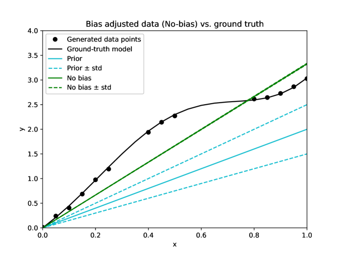
It can be observed that the prediction has converged close to a Dirac’s delta distribution due to the measurement noise being prescribed with a small variance. The model cannot represent the measurements because of model discrepancy. Uncertainty is also underestimated due to such discrepancy. Additionally, the unbiased approach provides a value of that makes the predictions at the observation points converge to the minimum Mean Square Error (MSE) with respect to the measurements, with a value of 3.34 and a standard deviation of 0.01. However, that value does not coincide with the norm between the generating process and the computational model over the domain of interest due to undersampling of the regions and . For reference, the optimal value of obtained using an loss is 3.6. This discrepancy further reduces the reliability of the inferred computational model far from the observation points, which is undesirable.
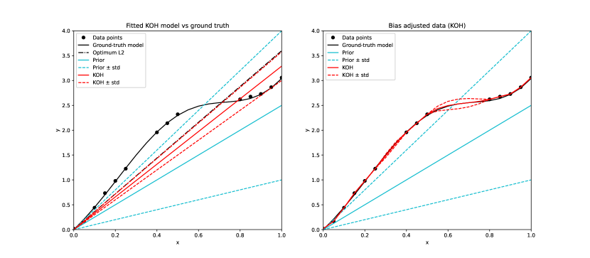
Next, the modularized version of KOH’s approach presented in Algorithm 1 is applied to the benchmark case. A GP with a Matérn kernel of is used to model the bias term . The correlation length for the bias GP is fixed to in the interest of a representative comparison between methods. In this case, the input is one-dimensional and requires only samples of for training, as the bias is defined for a given and will be newly trained at every MCMC evaluation. Consequently, the training set is generated at every sample of and is composed by the positions of the measurements as input, and their corresponding residuals for a given as output. Note that for this approach, the anchor points of the GP is always the input set . The fitted parameters can be observed in Table 1, and its fitted and bias-corrected responses are represented in Figure 2. The bias is a GP regressor, therefore for the case of just one measurement per observation point and given a sufficient kernel, the bias-corrected predicted response interpolates the observations. However, in the regions without measurements, the response presents a significantly larger bias. The bias itself can be used as a quantification of the model uncertainty.
As expected, one of the biggest caveats for this approach is the identifiability problem that arises between the latent parameter and the bias term. By adding a highly non-linear bias, the optimal solution for this simple 1D case would be the fitted parameter collapsing to a Dirac’s delta distribution with a value of 3.6 for the loss and the bias term compensating only the difference between the observations and the linear model. However, this is not the case, as the posterior predictive does not collapse despite the convergence of the MCMC process. This is explained due to the lack of identifiability between latent parameters and bias, still present in the modularized version of KOH, as the same improvement in the likelihood from Equation 7 can be achieved by modifying the parameter towards the optimum to minimize the residuals or towards values that improve the variance of the GP.
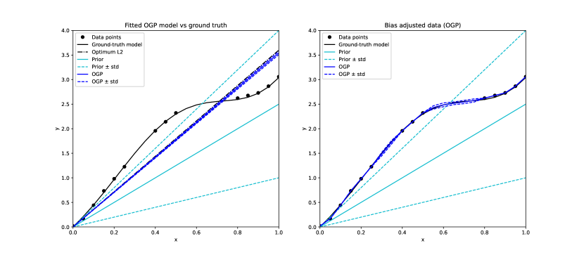
Analogously to the other approaches, OGPs are implemented for the simple 1D case. The only difference compared to KOH’s is the imposition of the orthogonality condition between the bias and the latent parameters at every evaluation of the MCMC loop. The required derivatives are obtained by applying a simple finite differences method with a central scheme and an increment step . Every other parameter remains the same as for KOH, i.e. the prior distributions and correlation kernel. The inference results can be observed in Table 1, and Figure 3 present the predictive results. The chosen metric is the loss, therefore the expected optimal value for is 3.6.
A comparison of the posterior predictive results is represented in Figure 4. It can be observed that none of the fitted models covers the data points without considering the bias. As expected, the no-bias and OGP approaches converge to a Dirac’s delta distribution, while KOH presents some variance. The analytical optimum value of using an -norm without noise is 3.6, and for the Mean Square Error (MSE) on the predictions is 3.33. In the perfect case, the point estimate for the maximum likelihood of should converge to a chosen optimum with almost no variance in the parameter. Thanks to the definition of the anchor points over the whole domain, only OGP is able to achieve such precision and allows controlling the norm with respect to which the optimum is calculated.
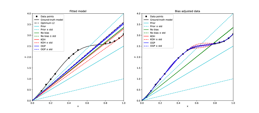
Alternatively, when observing the bias-corrected prediction, all the methods that include the bias are able to cover the observations in the confidence region. KOH and OGP interpolate over the measurements and present a very low variance between them. This is expected, as they are best fitting GPs for the residuals between computational model and observations using a maximum likelihood estimator for .
Altogether, OGP presents the best behaviour at the expense of additional computation time. The running times for each approach on 4 CPUs of an AMD EPYC 74F3 processor and 8 GB of RAM are presented in Table 2. It can be observed that KOH and OGP multiply by more than 33 and 45 times respectively the computation time in comparison to not considering bias. For KOH and OGP, this increment comes from the training of the GP for the bias at every evaluation of the MCMC chain, with additional time in the case of OGP for the evaluation of the derivatives and setting the orthogonal prior. It is expected that, for more complex cases, the largest time is spent in evaluations of the model instead of in the training of the bias, whose computation time should not increase for KOH in comparison. For OGP, it would depend on the availability of the derivatives and the choice of anchor points, which would dictate the required additional model evaluations. In comparison, these approaches would be relatively more efficient for such complex cases.
| Method | Time (s) |
|---|---|
| No bias | 3.3 |
| KOH | 110.4 |
| OGP | 151.6 |
3.2 Bias identification with heteroscedastic noise
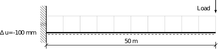
This case aims to reflect the influence of model bias in the estimation of heteroscedastic noise. Two models are differentiated to this end: one simple cantilever beam under a deterministic load condition that is used as the prescribed computational model and another one biased and with a stochastic load used to generate the data. The objective is to infer the value of the Young’s modulus for the computational model based on observations obtained from the biased one. This simplification mimics the situation of a testing load on a concrete cantilever bridge. The computational model supposes that only the experimental load is present in the real bridge, while the observations may have been collected with additional loads on the bridge or even with traffic. Additionally, it is supposed that a deficient placement and setting of the sensors leads to an additional displacement of mm for every measurement. These extreme additions are introduced for illustrative purposes, but comparable effects are observed regularly in real implementations of bridge monitoring systems, especially if the model updating is done with data from the bridge in service.
Both models correspond to a FEM representation of such a bridge as a 2D cantilever beam of length m and height m, discretized with quadrilateral linear elements. This represents half of the span of a bridge with constant a cross-section. The measurements will predict the deformation of the beam under a load at the free end with a simple linear elastic material law. The load represents a typical static test truck of 100 kN. The assumed width of the bridge is and its Poisson’s ratio is 0.2. Young’s modulus is the subject of this study, but in general, it will have a base value of 30 GPa. A diagram for the model is represented in Figure 5.
The complex generative model includes the additional prescribed displacement at the fixed boundary, simulating a displacement at the abutment or a deficient setting of the sensors. Additionally, in contrast with the deterministic load for the computational model of 100 kN, the generative model adds a stochastic component. The result is a constant force of 100 kN plus a random draw from a log-normal distribution with mean 20 kN and standard deviation 6 kN. This variability represents a simplification of the additional load from a vehicle over the bridge. Vertical displacement measurements are obtained at virtual sensor positions situated at m and m. The simulation is repeated 20 times, each with a different realization of the load, generating as many measurements per observation point. A prescribed Gaussian noise of zero mean and standard deviation of m is added to the measurements to simulate typical sensor noise.
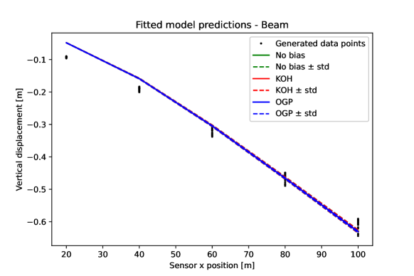
In this case, the virtual sensors cover sufficiently well the observation domain, therefore the fitted latent parameters are similar with and without bias. However, two impactful sources of error have been introduced: the prescribed displacement at the boundary and the variation in the load. They create respectively a discrepancy in the model’s response compared to the measurements and additional noise with physical meaning that cannot be explained a priori. It is not possible to fully represent these effects without considering a bias term. First, the aforementioned discrepancy can be directly estimated by including the bias analogously as in the simple 1D case: adding it to the output as a GP with the same combination of constant and Matérn kernel. Second, to allow the same GP to consider multiple measurements per sensor coordinate, a noise-enabled kernel must be employed. Due to the noise coming from the variation in the load, its amplitude must reflect the physical behaviour of the beam, therefore the noise is expected to vary in scale at the different sensors. This requires employing a heteroscedastic noise component added to the kernel, whose parameters are trained during the phase where the bias is fitted. Such a component is using the heteroscedastic kernel implemented in gp_extras45. A fixed homoscedastic white noise component with a value of 1e-12 m is added to avoid numerical inconsistencies due to the proximity to zero noise at the sensors near the cantilever boundary. The additional prescribed sensor noise is included in the regression kernel. Effectively, both the homoscedastic and heteroscedastic parts of the kernel will represent the same noise in the displacements produced by the load variability, which is expected to be larger than 1e-12 m at any sensor. Therefore, prescribing a constant homoscedastic part does not substantially impact the results, while increasing the numerical stability of the inference procedure. The additional derivatives required for OGP’s approach will be calculated using a central finite difference scheme with a step of GPa. An alternative popular approach for estimating this noise term in the absence of bias is to include it as a parameter to be inferred. This approach increments the number of latent parameters, does not address the model discrepancy and requires prior information on the noise that is not generally available. Nevertheless, it will be applied in the case with no bias in the interest of a more detailed comparison, providing further noise estimation capabilities.
An MCMC algorithm is used to infer following the methodologies previously. The latent variable is modelled with a prior normal distribution . In the case without bias, the noise term is defined with a uniform prior between 0 and 0.8 to allow any possible range of values. The MCMC algorithm is run for 500 steps with 100 additional steps of burn-in. The results can be observed in Figures 6 and 7. The summary statistics are displayed in Table 3.
| Group | Parameter | Mean | SD | HDI3% | HDI97% | MCSE | MCSE | |
|---|---|---|---|---|---|---|---|---|
| No bias | 1.486e+10 | 4.838e+08 | 1.391e+10 | 1.579e+10 | 3.999e+07 | 2.833e+07 | 1.070e+00 | |
| No bias | 5.900e-02 | 5.000e-03 | 5.100e-02 | 6.800e-02 | 0.000e+00 | 0.000e+00 | 1.070e+00 | |
| KOH | 1.521e+10 | 4.907e+08 | 1.428e+10 | 1.609e+10 | 3.609e+07 | 2.561e+07 | 1.040e+00 | |
| OGP | 1.470e+10 | 7.393e+07 | 1.459e+10 | 1.483e+10 | 1.177e+07 | 8.384e+06 | 1.170e+00 |
Convergence is achieved with every method in the chosen number of steps. For the approach without bias, the noise is inferred as an extra latent parameter. It must be noted and do not allow for a unique identification of such parameters due to the effect of the model discrepancy. Nevertheless, the convergence is apparent. Independently of the scale of the Gaussian noise , the fitted model will not be able to replicate the generated dataset. In comparison with the real Young’s modulus with a mean of 30 GPa and a standard deviation of 10 GPa, the inference procedure converges to a mean of around 14.9 GPa and standard deviation 0.5 GPa, which means an error of more than 50%. This relatively large difference is expected, as the predictions will never be able to accommodate the observations due to the prescribed displacement in the generative process. To obtain predictions closer to the observations, the computational model tends to become less stiff to accommodate the offset in the observations. The magnitude of the inferred noise without bias remarkably ranges between 0.051 and 0.068 m. With these values, it would fail to represent the noise both near the fixed end, close to zero, and at the free end, of approximately 0.025 m for the sampled data. Therefore, these predictions from the fitted model do not guarantee that the computational model reflects the real system, which is a requirement in the implementation of digital twins.
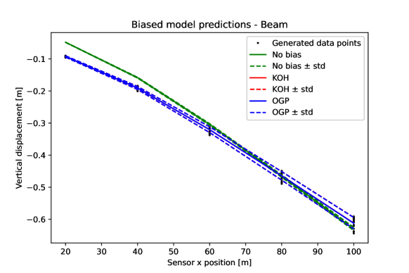
Similarly, the method that adds a bias term following KOH’s approach converges to a fitted Young’s modulus of mean 15.2 GPa and a standard deviation of 0.5 GPa. Once again, the system converges to the optimum fitting value that compensates for the deviation, not being able to represent the real generative process. The bias correction is consequently applied to the maximum-likelihood estimator of the fitted model, which generates corrected predictions. The key difference is the introduction of the heteroscedastic noise kernel, which allows capturing the variability in the observations.
Alternatively, adding the bias term as an OGP leads to a slower convergence measured by the Gelman-Rubin diagnostic. Imposing the orthogonality condition in the kernel with a noise component leads to GP kernel proposals that may not be able to fit the observations efficiently for some samples. To avoid this effect, the non-orthogonal part of the kernel could be adapted with a larger correlation length and scale, instead of using the same as in KOH’s approach. In the interest of an equivalent comparison, the chosen kernel prior was the same for both approaches. Despite this slightly larger of 1.17 after 500 MCMC steps, the OGP approach reasonably converges to a value of 14.7 GPa with a standard deviation of around 0.07 GPa, analogously to the other approaches in mean but with a decreased uncertainty. The noise structure and bias correction are equivalent to that presented in KOH’s approach. Nevertheless, the MCMC algorithm takes more than 5 times longer to evaluate due to an inefficient differentiation scheme and the introduction of poorly behaved priors for samples with extreme values. Due to the heteroscedastic noise kernel, which introduces a noise hyperparameter for each of the sampled positions, the training of the bias OGP may fail to converge more often when the strict orthogonality condition prevents finding the extended set of optimum noise hyperparameters. This could be improved by relaxing the orthogonality condition, which is possible by adjusting the fixed parameters of the Matérn kernel to increase the reach of the non-orthogonal part of the GP.
In comparison, the three approaches converge to a similarly wrong value of Young’s modulus in the fitted model due to the inability of the computational system to reflect the observations with the additional deformation. The optimal value for such that either the MSE or the loss between observations and predictions are minimized is around 14.8 GPa, which is approximately reached by each of the approaches. As both MSE and -optimum values are relatively close, it was expected that both the OGP and the unbiased method converge to a similar value. KOH’s approach tends to those same values, as these optimum parameters would provide the best-fitting bias distribution for the chosen GP prior. Adding the noise as a tunable parameter in the approach without bias does not improve the result nor quantify the real noise at the output. Contrarily, adding the bias term as in either approach allows the correction of the bias and quantifies the noise reliably. In this case, there is no apparent benefit of using OGP over KOH despite its larger computational times (see Table 4), as the chosen prior for KOH leads to the same optimum. As the bias term is directly applied at the output of the system, the value of does not reflect the one in the generative model and therefore could not be used for derived QoI that depend on it.
| Method | Time |
|---|---|
| No bias | 30 min |
| KOH | 4 h 50 min |
| OGP | 21 h 27 min |
The key feature highlighted by these results is the capacity of the bias term to represent a deviation of a biased model from reality. The noise in the approach without bias term cannot be quantified appropriately due to the existing discrepancy, while KOH can reliably correct the prescribed displacement and infer the noise produced by the variations in the material. This physical noise component of the observations is included as part of the model bias, which agrees with the assumption that the model’s Young’s modulus employed in the digital twin is unique and deterministic. The inability of the model to represent stochastic responses is compensated by a noise-enabled bias with a modified kernel. Without this bias term, the model response variance remains unknown and the model predictions are not able to represent the reality of the system. It is shown that a heteroscedastic noise kernel can be used in the bias to this end in a non-intrusive manner, without modifying the model or the inference schemes. Samples from this posterior predictive distribution can be used in the context of a digital twin to provide information on points where no observation is available or to further derive QoI based on such predictions. The stochastic nature of the bias-corrected predictions provides a quantification of the uncertainty in the observations produced by the variability of the real system, and not only due to the indeterminacy of the model parameters. For example, large variations in the bias could indicate a deficient testing setup, or in this case, the inclusion of loads not considered in the model.
3.3 Bias identification incorporating additional environmental conditions
3.3.1 Case definition
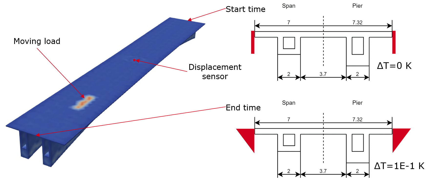
The objective of this case is the inclusion of additional information on the environmental conditions in the bias identification applied to a real use case. Consequently, the final use case illustrates their implementation on a simplified model of an actual bridge: the Nibelungenbrücke in Worms, Germany, displayed in Figure 10. The research initiative "Schwerpunktprogramm 2388: SPP Hundert Plus", within which this work is included, aims to monitor and eventually prolong the remaining life of the bridge through novel digital approaches, in particular the implementation of digital twins46. Therefore, a model using a simplified version of Nibelungenbrücke’s geometry is developed, paying special attention to its use in such a digital twin. The objective of this use case is the evaluation of the model bias approaches in a digital twin setting and the inclusion of additional variables, therefore the modelling of the bridge has been extremely simplified and would not necessarily coincide with an accurate representation of the real one. It must be particularly noted that the spans of the real bridge should be represented as cantilever structures attached at the center of the spans and with the pilots as supports. However, the simulation of a span will be represented by a simply-supported structure of the full span length for illustrative purposes. This choice has no impact on the conclusions extracted from this benchmark with respect to the application of biased approaches. The work presented in this paper will use simulation models for both generating the virtual observation data and predicting results. Measurements from the bridge are expected in the future, which will allow further testing of the methodology under real sensor observations. However, the validation with real data remains out of the scope of this paper, and this benchmark reflects the real system with many simplifying assumptions.

The first span of the bridge is chosen for the simulation model. It is represented as a solid 3D Finite Element (FE) box-girder model with variable cross-section. The dimensions of the model correspond to those indicated in available drawings47 and databases48, with a span length of 95,185 m, span width varying between 14 m at the centre and 14.64 at the pilots, deck thickness of 0.25 m, cross-section height at pilots of 6.5 m and of 2.5 m at the middle of the span. The mesh is a tetrahedral 3D solid unstructured mesh with linear Lagrangian elements, with characteristic length between 0.2 and 2.0 m. The material is modelled using a purely linear elastic constitutive law with a Young’s modulus of 40 GPa, a Poisson’s ratio of 0.2 and a density of 2350kg/m3. Simply supported boundary conditions are considered at the end surfaces, where the bottom edge of the supports is fixed in displacements, as represented in Figure 9. The resulting model has 3530 nodes, which is equivalent to 10580 Degrees of Freedom (DoFs) and 20669 elements. A more complex model is possible, but it would not enhance in any way the conclusions from this study.
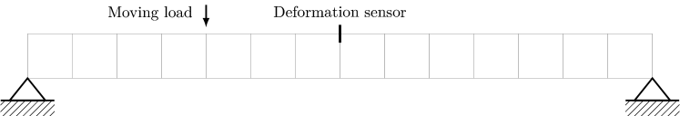
The virtual experiment will represent an influence line test under a moving load. A virtual displacement sensor is placed at the middle point of the span on the surface of the deck to measure vertical displacements. Then a simulated moving load is applied passing over the bridge, and the measurements of the sensor are recorded for every load position. In this case, the load represents a truck of 10 t, 8 m long and 3 m wide moving at a speed of 0.5 m/s over the bridge. This load is modelled as a rectangular surface load of the same dimensions, taking the front line of the truck as the reference for its position. The displacements are recorded with a sampling rate of 2 s. The plot of the observations recorded by the sensor during the time the truck is passing over the bridge is considered the influence line of that load. This line can be used to infer parameters of the bridge such as its Young’s modulus. The calculation of the influence load does not consider any inertial effects, hence the simulation is a purely static one evaluated with different load locations.
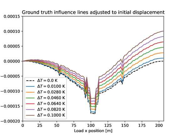
The computational model to be tuned will be the simulation to generate the influence lines and the parameter of interest that must be inferred will be the Young’s modulus used in the simulation. An additional temperature effect is added only for the generation of the dataset, introducing a discrepancy between the generated data and the computational model. During the time that the truck would pass over the bridge, it is reasonable to assume a change in the temperature of the top surface of the deck49. This can be, for example, due to the incidence of the sun over it. At the start of the experiment, we support a constant stationary temperature over the whole bridge. The top part of the deck will increase its temperature due to the transient effect of the heat on the surface, while the bottom part will remain unaffected due to the short timescale that prevents fast heat propagation. This situation generates a linear temperature gradient along the cross-section of the deck, which implies further thermal strains that will be identified by the sensor. These strains are introduced in the linear elastic model with a thermal expansion coefficient . A diagram of the experimental set-up is represented in Figure 10. In practice, the difference in temperature between the start and end of the measurements on the top of the deck is measured, supposing a linear evolution of it. In this case, we run 6 simulations with temperature differences between start and end of [1e-2, 2.8e-2, 4.6e-2, 6.4e-2, 8.2e-2, 1e-1] K. This corresponds to a change of between 5 and 15 K in a period of 12 h, which is in line with expected values in similar applications50. The observed influence lines for this experiment are represented in Figure 11. The base case with no temperature difference has been represented in the figure as a reference, but will not be fed as data to the model for its calibration. Notably, the deformation is greater than zero at the end of the simulation when the temperature gradient is introduced. This effect cannot be replicated by the original model, as the only external load applied on the system comes from the passing truck, which at the end of the measurements is no longer over the bridge. Therefore, all the fitted models will predict zero deformation at the end of the simulation. No additional noise is introduced in the system, although the same methodology of the previous benchmark could be applied.
3.3.2 Models without temperature consideration
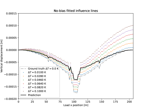
Analogous to the previous benchmark cases, an MCMC algorithm is used to infer Young’s modulus from its influence lines. In this case, is prescribed with a prior log-normal distribution with parameters and . The equivalent mean for is approximately 35.8 GPa, which lies within a reasonable range of the real value of 40 GPa. The MCMC algorithm is run for 1000 steps with 200 steps of burn-in. For the case without bias, the 6 influence lines are treated as independent datasets, each of them weighted equally in the likelihood calculation. For KOH and OGP, an additive bias term modelled as a GP is included in the computational model. First, the bias GPs will be implemented analogously as the previous cases, without extending the input domain, following the algorithms from Section 2. In the case of KOH’s approach, the kernel of the bias GP is a Matérn one with a fixed lengthscale and a fixed standard deviation , multiplied by a constant valued kernel that is variable. For OGP, this same kernel is applied as the base to which the orthogonality condition is imposed. The load position for each observation is used as training input for the bias, and the residual of a given observation for the predictions is taken as output. Notice that there are 6 distinct observations for each load position with their corresponding residuals, one for each experimental series. These observations are indistinguishable from each other for the model and the GP, as they do not contemplate changes in the temperature. The predicted bias correction for a given load position will therefore be unique, independently of the temperature difference at the end of the experiment.
| Group | Mean | SD | HDI3% | HDI97% | MCSE | MCSE | |
|---|---|---|---|---|---|---|---|
| No bias | 5.785e+10 | 1.952e+05 | 5.785e+10 | 5.785e+10 | 2.105e+04 | 1.494e+04 | 2.950e+00 |
| KOH without Temperature | 3.998e+10 | 1.698e+08 | 3.966e+10 | 4.026e+10 | 1.699e+07 | 1.206e+07 | 1.080e+00 |
| KOH with Temperature | 4.000e+10 | 4.321e+06 | 3.999e+10 | 4.001e+10 | 3.596e+05 | 2.548e+05 | 1.050e+00 |
| OGP without Temperature | 5.783e+10 | 6.487e+07 | 5.772e+10 | 5.797e+10 | 1.506e+07 | 1.082e+07 | 1.240e+00 |
| OGP with Temperature | 5.778e+10 | 3.703e+08 | 5.778e+10 | 5.800e+10 | 5.823e+07 | 4.169e+07 | 1.580e+00 |
Inference results can be observed in Table 5. Due to the absence of a non-prescribed noise latent parameter, the approach without bias tends to minimize the MSE for each load position. Therefore, it converges to a value of around 57.8 GPa with strong certainty, which implies an error of 44.5% with respect to the real value. The resulting influence lines of fitting the model without including a bias term are represented in Figure 12. The fitted model is not representative of the real system despite its certainty. This situation renders the obtained results unreliable and inaccurate. If a noise term were to be included, still the system would not reflect the reality, as the inferred parameters would not coincide with the real ones, and the generated predictions could not be used for making decisions on the behaviour of the bridge. In particular, the non-zero response at the end of the experiment despite the absence of load on the system cannot be replicated without considering a bias.
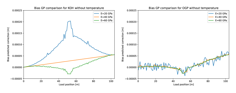
Alternatively, both KOH and OGP approaches are able to overcome the limitations previously mentioned, see Figures 13 and 14. In particular, the bias-corrected response in both cases fits exactly the MSE of the observations at each load position. Due to the flexible bias term, the corrected prediction is not limited to representing a null displacement at the end of the experiment, allowing for a better representation of the observations. Remarkably, the fitted parameter obtained with KOH’s approach converges with almost no uncertainty towards the real value of 40 GPa, while for OGP it tends to 57.9 GPa, a similar value to the one for the approach without bias. This disparity can be explained by observing the behaviour of the bias predictions for different values of , as represented in Figure 15. For the case of KOH’s approach, the optimization objective is the value of with the "best-fitting bias", which translates in this case to a minimization of the marginal log-likelihood of the bias GP for a given . Following Equation 7, large residuals and large covariance values are penalized. Observing Figure 15, it can be appreciated that GPa generates a very smooth set of residuals due to the linear nature of the temperature increase over time, which greatly reduces the values of . The reduction in the residuals for values with larger does not compensate for the increase in variance, which results in KOH eventually converging to a value close to GPa. It must be remarked that this is true for the chosen combination of kernel and observations due to the regularity and smoothness of the bias introduced by the temperature difference but is not generally true for any system. As mentioned before, it is not possible to control a priori the optimality metric of KOH’s approach for an arbitrary choice of priors. Nevertheless, bias from physical sources is expected to be relatively smooth, which can favour such an approach.
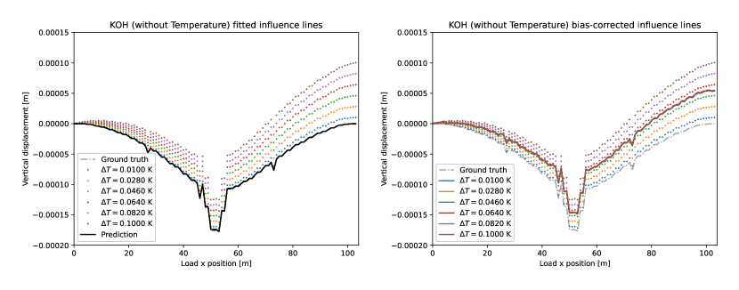
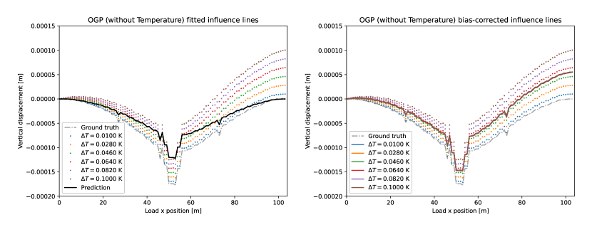
In comparison, the imposition of the orthogonality condition onto the bias GP kernel leads the distribution of to converge towards the MSE. It must be noted that the correction generated by the bias from OGP only fits the observations in the case of an optimal value of . The orthogonality condition restricts -through a modification of the covariance matrix- the function space that can represent the bias correction. In this case, as the derivative of the computational model with respect to the Young’s modulus does not change much in the studied range of , the orthogonal kernel remains almost constant for every evaluation. In particular, the functions generated by the bias GP will resemble the case where is optimal, the MSE of the observations. Additionally, the orthogonal kernel translates into an impossibility of the bias GP to be trained to fit residuals that would be improved by a modification of the latent parameter. In this case, it means that, for an arbitrary , the bias will be able to correctly compensate for the discrepancy at the end of the experiment (which can only be explained through the bias) but not the values when the load is at the center of the span (which can be largely altered by a modification in the value of ). These diminished effects of the bias on some parts of the domain imply larger covariance values due the inability to cover the observed residuals with members of the imposed function space. The increased loss of smoothness due to high variance for values of far from 57.8 GPa can be observed in Figure 15. Larger variations in the derivative of the computational model with respect to would lead to more dissimilar realizations of the bias response mean. Nevertheless, the convergence to the optimum is achieved thanks to diminishing covariances obtained by the fulfilment of the orthogonality condition in values closer to the MSE. The mean of the bias response corresponds with the residuals for that value in the whole domain of application.
Nevertheless, the predictions obtained through the approaches with bias still present some limitations. First, the system cannot reproduce the observations and only performs a regression on the different experimental sets. Second, if the bias had a more complex non-linear behaviour with respect to increments in temperature difference between series, the bias would not be able to reflect it. Finally, the obtained bias does not provide insight into the quality of the model with respect to the temperature differences at the end of the experiment, as it only corrects the displacement over time to achieve the MSE of the training observations, not considering the end difference temperature for the associated experiment. These shortcomings can be mitigated by extending the input of the domain for the bias GP.
3.3.3 Models with temperature consideration
In this case, the bias GP will depend on the temperature difference as well. Its main attraction is to include information that may be relevant to the process without modifying the computational model itself. This extension of the domain of interest through the bias allows weighting in the influence of the temperature difference in the inference process while providing insight into the potential model deficiencies. Therefore, the bias GP will be trained on pairs of the form , where is the current load position and is the associated end temperature difference for a given observation. This bias can consequently be represented by a response surface with a 2D input and a 1D output. Each series of observations is part of the same experiment with an associated measured at the end of it. The intermediate temperatures are not available, therefore all the observations will share the final as their coordinate in the extended domain. The training of the bias term and the inference procedures are implemented following the algorithms from Section 2. In this case, an additional scaling of the domain and the residuals is applied to improve the fitting of the bias GP. The GP inputs are scaled such that the original domain is transformed to . The residuals and derivatives are multiplied by a factor of 100 during the training to increase numerical stability. The originally small residuals produced by the displacements lead to values of the variance close to machine precision after scaling the time domain, which leads to numerical instabilities of the GP training. To compensate this effect, the scaling factor in the residuals is chosen in the same order of magnitude as the original time length. The same previous kernels are applied for KOH and OGP, extending them to accept 2D inputs.
The results of including temperature information in KOH’s approach can be observed in Figure 16. Analogously to the case without temperature, the inferred tends to 40 GPa due to the linearity in the bias with respect to the temperature increments and in time. A comparison of the bias response surface for =40 GPa and =60 GPa is presented in Figure 17. As in the previous evaluation, the reduction of the residuals provided by larger values of does not compensate for the increase in complexity, which is translated to larger values for the determinant of the covariance matrix and, consequently, smaller likelihoods. However, if the predictions are corrected by the learnt bias term trained on the MLE of , it is possible in this case to regenerate the observations for each temperature gradient. This corrected model can be used for generating influence lines for other temperature gradients in the training range. Nevertheless, the inferred bias cannot be trusted for other applications, as it is defined only on the predicted influence lines, but it can be useful for identifying trends in the model discrepancy. An analysis of the bias contour lines and their variance such as the one presented in Figure 18 points out increasing uncertainties with larger temperature differences and at the end of each experiment. Additionally, the largest variances occur between samples with different temperature increments. These observations coincide with the expected behaviour of the model. If a noise component were to be inferred additionally, the variance would be significantly reduced in comparison with the case without temperature awareness, as the observations would be considered independently and not as realizations of the same distribution.
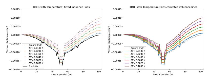
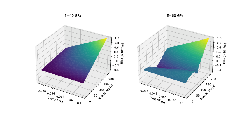
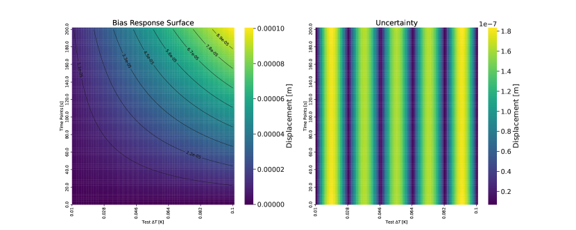
Finally, the influence lines and corrected predictions for OGP’s approach are represented in Figure19. The orthogonal prior imposed in OGP’s approach favours convergence to the sampled that minimizes the prescribed loss between computational and generative models, the loss in this case. As the computational model is not aware of the temperature gradient, the observations are sufficiently detailed and the anchor points of the computational model coincide with the observation points, minimizing such a loss is almost equivalent to minimizing the MSE, analogously to the case where temperature is not included in the bias. Consequently, the optimal value of obtained by imposing an OGP on the bias coincides with the best-fitting computational model to the observation but disregards the additional information introduced by the temperature gradient. In this case, this means a tendency towards 57.8 GPa. The comparison of the bias response surfaces represented in Figure 20 presents an analogous behaviour as the case where the temperature is not included, where the fitness of the GP is driven by its variance due to the small changes in the derivative of the computational model with respect to in the chosen domain. It is remarkable that, as shown in Figure 21, the bias response surface presents relatively low uncertainty, despite not being able to fit the observations. This surface informs about the distribution of the discrepancy between model prediction at the MSE and the measurements, which could be useful to identify regions of low certainty in the input parameter space, indicating deficiencies in the model. Nevertheless, as the inference converges to the optimum value of , the bias-corrected predictions are able to reflect the observations, including the temperature effect.
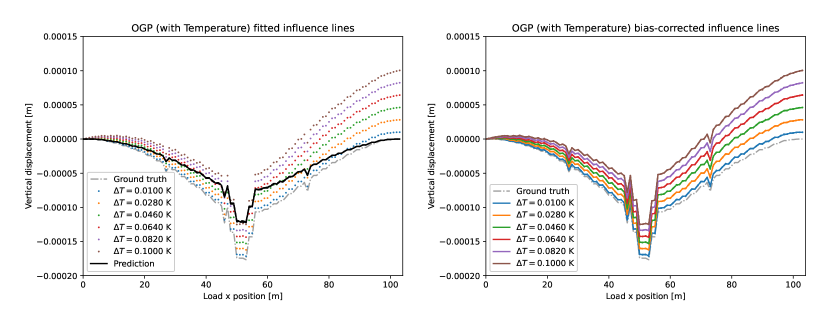
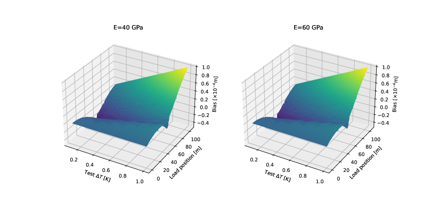
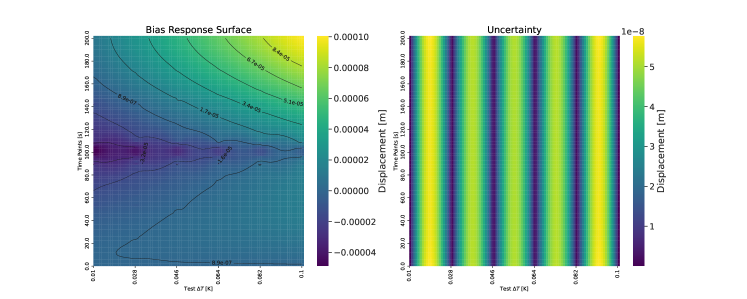
In comparison, KOH and OGP outperform the classical approach with and without considering the temperature increment in the bias. If the model does not include information about the temperature, the bias correction allows to regenerate the MSE of the observations and provides insight into the evolution of the discrepancy depending on the load’s position. However, the inclusion of the temperature differences in the bias informs of deficiencies in the model with respect to them, as well as the distribution of the uncertainty. Remarkably, this is achieved without needing to modify the computational model, only making use of already available information. The insight provided by the inclusion of temperature can be valuable for the design of future measurement campaigns or for the identification of potential improvements in the computational model, which are of great relevance in the context of digital twins. Additionally, if the computation times presented in Table 6 are considered, the cost of implementing KOH’s approach to extend the model to include the temperature difference is negligible in comparison with the approach without temperature or even without bias. Most of the computational time is spent in evaluating the model to generate the influence lines for each sample while training the GP on as needed for KOH’s approach is faster in comparison. OGP’s additional time comes from the necessity to solve the system several times per evaluation to calculate the gradient. A more efficient differentiation approach would reduce the difference in time between OGP and KOH. In conclusion, KOH’s approach should be applied when possible to extend the system through the bias due to its reduced computational cost, simple integration and valuable insights. It is possible that for more complex cases, where more than one extra coordinate is introduced, this approach may incur further identifiability issues.
Another relevant consideration is the capacity of the predicted response to fit the observations. The Mahalanobis distance can be used to compare the posterior distribution of the bias-corrected responses for each approach with the observations. As the posterior distributions are relatively narrow, the Mahalanobis distances is almost equivalent to the Euclidean one, while the latter is numerically easier to compute due to the absence of a badly conditioned inverse matrix. The Euclidean distance for each approach with respect to the observations is presented in Table 6. The approaches with bias and no temperature information show slight improvement over the approach without bias due to their capacity to provide predictions out of the limits of the computational model, such as the zero displacement at the end of the experiments. However, the largest improvement comes from the inclusion of the temperature differences in the bias, as these approaches are able to fit every experiment series. In the absence of prior information, these distances can be used to assess the impact of introducing the temperature differences in the system and to guide further refinements of the digital twin simulation model. As expected, there is a clear benefit in this case for introducing the available temperature information.
| Method | Time | Euclidean distance |
|---|---|---|
| No bias | 5 h 15 min | 4.77e-4 |
| KOH without temperature | 5 h 21 min | 4.49e-4 |
| KOH with temperature | 5 h 30 min | 9.41e-9 |
| OGP without temperature | 15 h 15 min | 4.46e-4 |
| OGP with temperature | 15 h 31 min | 1.57e-6 |
4 Conclusion
In this paper, we have proposed solutions to some of the main challenges for the reliable implementation of simulation-based digital twins of bridges. A Bayesian inference framework is often considered the best option for the calibration of the model parameters. However, we observed that classical approaches led to overconfident models whose response does not replicate the observations and whose behaviour does not correspond to the physical system. This renders them unsuitable for their use in digital twins of critical infrastructures such as bridges, where fidelity, robustness and accuracy are key to guarantee their safety. The root of this inadequacy stems from the inability of computational models to recreate the infinitely complex reality to its fullest extent. We proposed the explicit introduction of a model bias term in the formulation and calibration of the digital twin to mitigate such an effect. Two different approaches were compared with the classical inference methodology, one with a modularized version of Kennedy and O’Hagan’s framework and one based on OGPs. Through three relevant use cases, we proved that biased approaches did not only compensate for the model bias but also provide new insight into model deficiencies. Additionally, we introduced two novel extensions to the model bias identification schemes to correctly quantify noise in the observations from unknown physical sources and to make use of complementary information.
First, when applied to a simple 1D case where model bias is present, the classical approach converged to a suboptimal parameter value with high certainty, despite not being able to fit the observations. Contrarily, both biased approaches were able to correct successfully the predictions to fit the observations, properly address the uncertainty and, for the case of OGP, to provide the optimal value for the latent parameter. In the context of digital twins, the introduction of the orthogonality condition allows for the use of fewer data point locations, i.e. sensors, while keeping control of the optimality of the solution. Additionally, the extension of the solution to the domain of the anchor points instead of the sensors generates reliable solutions at points of interest where no data is available. This is generally done at the expense of longer computational times and model evaluations at those points, which can be a challenge for complex and expensive simulation models.
Next, the three methodologies were applied to a stochastic cantilever beam with model bias and additional noise from a non-prescribed physical source. Although the estimated Young’s modulus differed from the real value in any case, only the biased approaches were able to estimate the noise and correct the predictions, but could not properly identify the noise due to the presence of model bias. Both KOH and OGP enable the introduction of homoscedastic and heteroscedastic noise kernels without modifications to the system or the inference procedure, which provides great flexibility. The introduction of such kernels has proven key to identifying noise under conditions of bias.
Finally, a test demonstrator example of the Nibelungenbrücke was implemented, where a discrepancy from a temperature difference was introduced to evaluate the ability of the approaches to include new information into the system. The extension of the model through the bias allowed us to gain relevant insight into the deficiencies in the model just by leveraging already available information. The computational cost of implementing KOH compared to not including the bias term is negligible for such a complex model, which makes this approach very promising for its implementation in digital twins of bridges.
However, one of the main challenges of the presented methodologies is the inability to assure the physicality of the inferred parameters due to the addition of the corrective bias term at the output of the predictions. The model itself is therefore not directly modified, and the corrections cannot be utilized for the calculation of different QoIs than the ones used for the calibration. Nevertheless, the generated bias and the corrected models allowed us to better understand the deficiencies present in the current model in a quantitative manner. Additionally, the evaluation of the presented frameworks under real measurements is required for validation of the exposed approaches in structures as-built. The complexity of sensor observations and the variation in environmental and operational conditions cannot be replicated with simulated data, therefore the evaluation of a definitive assessment of their performance is only possible under such conditions. Furthermore, the integration of these methodologies in a unified digital twin of a bridge presents additional challenges related to accessibility, ownership, connectivity and cybersecurity that should not be understated.
In conclusion, a suitably selected biased approach outperformed classical implementations in every case, proving their effectiveness in the reduction of the effects associated with the model bias. OGPs provide optimal results at the expense of increased computational times when the model already considers the domain of interest, while KOH’s approach allows for the extension of such domain with additional information. The choice of one or the other will depend on the complexity of the model and its intended use.
References
- 1 Tao F, Qi Q. Make more digital twins. Nature. 2019;573(7775):490–491. doi: 10.1038/d41586-019-02849-1
- 2 Sharma A, Kosasih E, Zhang J, Brintrup A, Calinescu A. Digital Twins: State of the art theory and practice, challenges, and open research questions. Journal of Industrial Information Integration. 2022;30:100383. doi: 10.1016/j.jii.2022.100383
- 3 Grieves MW. Virtually Intelligent Product Systems: Digital and Physical Twins. In: , , Sunrise Valley, United States: American Institute of Aeronautics and Astronautics, Inc., 2019:175–200
- 4 Lu Q, Parlikad AK, Woodall P, et al. Developing a Digital Twin at Building and City Levels: Case Study of West Cambridge Campus. Journal of Management in Engineering. 2020;36(3). doi: 10.1061/(asce)me.1943-5479.0000763
- 5 Chinesta F, Cueto E. Empowering engineering with data, machine learning and artificial intelligence: a short introductive review. Advanced Modeling and Simulation in Engineering Sciences. 2022;9(1). doi: 10.1186/s40323-022-00234-8
- 6 Koutsourelakis P. A multi-resolution, non-parametric, Bayesian framework for identification of spatially-varying model parameters. Journal of Computational Physics. 2009;228(17):6184–6211. doi: 10.1016/j.jcp.2009.05.016
- 7 Koutsourelakis PS. A novel Bayesian strategy for the identification of spatially varying material properties and model validation: an application to static elastography. International Journal for Numerical Methods in Engineering. 2012;91(3):249–268. doi: 10.1002/nme.4261
- 8 Mahnken R. Identification of Material Parameters for Constitutive Equations:1-21; John Wiley & Sons, Ltd . 2017
- 9 Martins J, Andrade-Campos A, Thuillier S. Comparison of inverse identification strategies for constitutive mechanical models using full-field measurements. International Journal of Mechanical Sciences. 2018;145:330–345. doi: 10.1016/j.ijmecsci.2018.07.013
- 10 Bruder L, Koutsourelakis PS. Beyond black-boxes in Bayesian inverse problems and model validation: applications in solid mechanics of elastography. International Journal for Uncertainty Quantification. 2018;8(5):447–482. doi: 10.1615/Int.J.UncertaintyQuantification.2018025837
- 11 Alvin KF. Finite element model update via Bayesian estimation and minimization of dynamic residuals. 1996.
- 12 Marwala T, Sibisi S. Finite Element Model Updating Using Bayesian Framework and Modal Properties. Journal of Aircraft. 2005;42(1):275–278. doi: 10.2514/1.11841
- 13 Ereiz S, Duvnjak I, Jiménez-Alonso JF. Review of finite element model updating methods for structural applications. Structures. 2022;41:684–723. doi: 10.1016/j.istruc.2022.05.041
- 14 Coelho Lima I, Robens-Radermacher A, Titscher T, Kadoke D, Koutsourelakis PS, Unger JF. Bayesian inference for random field parameters with a goal-oriented quality control of the PGD forward model’s accuracy. Computational Mechanics. 2022. doi: 10.1007/s00466-022-02214-6
- 15 Rosafalco L, Torzoni M, Manzoni A, Mariani S, Corigliano A. Online structural health monitoring by model order reduction and deep learning algorithms. Computers & Structures. 2021;255:106604. doi: 10.1016/j.compstruc.2021.106604
- 16 Rózsás Á, Slobbe A, Martini G, Jansen R. Structural and load parameter estimation of a real-world reinforced concrete slab bridge using measurements and Bayesian statistics. Structural Concrete. 2022;23(6):3569–3600. doi: 10.1002/suco.202100913
- 17 Titscher T, van Dijk T, Kadoke D, Robens-Radermacher A, Herrmann R, Unger JF. Bayesian model calibration and damage detection for a digital twin of a bridge demonstrator. Engineering Reports. 2023. doi: 10.1002/eng2.12669
- 18 Andrés Arcones D, Weiser M, Koutsourelakis FS, Unger JF. A Bayesian Framework for Simulation-based Digital Twins of Bridges. ce/papers. 2023;6(5):734–740. doi: 10.1002/cepa.2177
- 19 Kaipio J, Somersalo E. Statistical and Computational Inverse Problems. Springer London, Limited, 2006.
- 20 McClarren RG. Uncertainty Quantification and Predictive Computational Science A Foundation for Physical Scientists and Engineers. Springer, 2018
- 21 Foreman-Mackey D, Hogg DW, Lang D, Goodman J. emcee: The MCMC Hammer. Publications of the Astronomical Society of the Pacific. 2013;125(925):306–312. doi: 10.1086/670067
- 22 Salvatier J, Wiecki TV, Fonnesbeck C. Probabilistic programming in Python using PyMC3. PeerJ Computer Science. 2016;2:e55. doi: 10.7717/peerj-cs.55
- 23 Carpenter B, Gelman A, Hoffman MD, et al. Stan: A probabilistic programming language. Journal of statistical software. 2017;76(1).
- 24 Olivier A, Giovanis DG, Aakash B, Chauhan M, Vandanapu L, Shields MD. UQpy: A general purpose Python package and development environment for uncertainty quantification. Journal of Computational Science. 2020;47:101204. doi: 10.1016/j.jocs.2020.101204
- 25 BAM . probeye. https://github.com/BAMresearch/probeye; 2023.
- 26 Oreskes N, Shrader-Frechette K, Belitz K. Verification, Validation, and Confirmation of Numerical Models in the Earth Sciences. Science. 1994;263(5147):641-646. doi: 10.1126/science.263.5147.641
- 27 Kaipio J, Somersalo E. Statistical inverse problems: Discretization, model reduction and inverse crimes. Journal of Computational and Applied Mathematics. 2007;198(2):493–504. doi: 10.1016/j.cam.2005.09.027
- 28 Kennedy MC, O’Hagan A. Bayesian calibration of computer models. Journal of the Royal Statistical Society: Series B (Statistical Methodology). 2001;63(3):425–464. doi: 10.1111/1467-9868.00294
- 29 Oberpriller J, Cameron DR, Dietze MC, Hartig F. Towards robust statistical inference for complex computer models. Ecology Letters. 2021;24(6):1251–1261. doi: 10.1111/ele.13728
- 30 Arendt PD, Apley DW, Chen W. Quantification of Model Uncertainty: Calibration, Model Discrepancy, and Identifiability. Journal of Mechanical Design. 2012;134(10). doi: 10.1115/1.4007390
- 31 Brynjarsdóttir J, O’Hagan A. Learning about physical parameters: the importance of model discrepancy. Inverse Problems. 2014;30(11):114007. doi: 10.1088/0266-5611/30/11/114007
- 32 Bayarri MJ, Berger JO, Liu F. Modularization in Bayesian analysis, with emphasis on analysis of computer models. Bayesian Analysis. 2009;4(1). doi: 10.1214/09-ba404
- 33 Menberg K, Heo Y, Choudhary R. Influence of error terms in Bayesian calibration of energy system models. Journal of Building Performance Simulation. 2018;12(1):82–96. doi: 10.1080/19401493.2018.1475506
- 34 Chong A, Menberg K. Guidelines for the Bayesian calibration of building energy models. Energy and Buildings. 2018;174:527–547. doi: 10.1016/j.enbuild.2018.06.028
- 35 Sargsyan K, Huan X, Najm HN. Embedded model error representation for Bayesian model calibration. International Journal for Uncertainty Quantification. 2019;9(4):365–394. doi: 10.1615/int.j.uncertaintyquantification.2019027384
- 36 Strong M, Oakley JE, Chilcott J. Managing Structural Uncertainty in Health Economic Decision Models: A Discrepancy Approach. Journal of the Royal Statistical Society Series C: Applied Statistics. 2011;61(1):25–45. doi: 10.1111/j.1467-9876.2011.01014.x
- 37 Chen G, Fan J, Dong S, Liu D. Strength uncertainty analysis of composite turbine blade with small sample size. Structures. 2021;33:1158–1179. doi: 10.1016/j.istruc.2021.04.059
- 38 Huan X, Safta C, Sargsyan K, et al. Global Sensitivity Analysis and Quantification of Model Error for Large Eddy Simulation in Scramjet Design. In: American Institute of Aeronautics and Astronautics 2017
- 39 Strong M, Oakley JE. When Is a Model Good Enough? Deriving the Expected Value of Model Improvement via Specifying Internal Model Discrepancies. SIAM/ASA Journal on Uncertainty Quantification. 2014;2(1):106–125. doi: 10.1137/120889563
- 40 Plumlee M. Bayesian Calibration of Inexact Computer Models. Journal of the American Statistical Association. 2017;112(519):1274–1285. doi: 10.1080/01621459.2016.1211016
- 41 Liu JS. Monte Carlo Strategies in Scientific Computing. Springer New York, 2004
- 42 Rasmussen CE. Gaussian processes for machine learning. MIT Press, 2006.
- 43 Gramacy RB. Surrogates: Gaussian Process Modeling, Design and Optimization for the Applied Sciences. Boca Raton, Florida: Chapman Hall/CRC, 2020. http://bobby.gramacy.com/surrogates/.
- 44 Gelman A, Rubin DB. Inference from Iterative Simulation Using Multiple Sequences. Statistical Science. 1992;7(4). doi: 10.1214/ss/1177011136
- 45 Metzen JH. gp_extras. https://github.com/jmetzen/gp_extras; 2016.
- 46 SPP: SPP 100+. Technical Univeristy of Dresden: www.spp100plus.de; 2023. Accessed November 18, 2023.
- 47 Pelke E, Zichner T. Ertüchtigung der Nibelungenbrücke Worms. Beton- und Stahlbetonbau. 2015;110(2):113–130. doi: 10.1002/best.201400082
- 48 Janberg N. Nibelungenbrücke. Structurae, International Database and Gallery of Structures https://structurae.net/en/structures/nibelungenbrucke; 2000. Last updated on February 5, 2016. Accessed November 18, 2023.
- 49 Wang D, Tan B, Wang X, Zhang Z. Experimental study and numerical simulation of temperature gradient effect for steel-concrete composite bridge deck. Measurement and Control. 2021;54(5-6):681–691. doi: 10.1177/00202940211007166
- 50 Xia Q, Zhou L, Zhang J. Thermal performance analysis of a long-span suspension bridge with long-term monitoring data. Journal of Civil Structural Health Monitoring. 2018;8(4):543–553. doi: 10.1007/s13349-018-0299-y
Author contributions
Daniel Andrés Arcones: methodology (lead), formal analysis (lead), software(lead), visualization (lead), original draft preparation (lead). Martin Weiser: conceptualization (equal), supervision (equal), review and editing (equal). Faidon-Stelios Koutsourelakis: conceptualization (equal), supervision (equal), review and editing (equal). Jörg F. Unger: conceptualization (equal), supervision (equal), review and editing (equal).
Acknowledgments
BAM is a senior scientific and technical federal institute with responsibility to the German Federal Ministry for Economic Affairs and Climate Action.
Financial disclosure
This work was funded through the project "C07 - Data driven model adaptation for identifying stochastic digital twins of bridges" from the Priority Program (SPP) 2388/1 "Hundred plus" of the German Research Foundation (Deutsche Forschungsgemeinschaft, DFG).
Conflict of interest
The authors declare no potential conflict of interests.
Supporting information
Additional supporting information may be found in the online version of the article at the publisher’s website.